Model Predictive Control with Environment Adaptation for Legged Locomotion

Abstract

Re-planning in legged locomotion is crucial to track the desired user velocity while adapting to the terrain and rejecting external disturbances. In this work, we propose and test in experiments a real-time Nonlinear Model Predictive Control (NMPC) tailored to a legged robot for achieving dynamic locomotion on a variety of terrains. We introduce a mobility-based criterion to define an NMPC cost that enhances the locomotion of quadruped robots while maximizing leg mobility and improves adaptation to the terrain features. Our NMPC is based on the real-time iteration scheme that allows us to re-plan online at $25\,\mathrm{Hz}$ with a prediction horizon of $2$ seconds. We use the single rigid body dynamic model defined in the center of mass frame in order to increase the computational efficiency. In simulations, the NMPC is tested to traverse a set of pallets of different sizes, to walk into a V-shaped chimney, and to locomote over rough terrain. In real experiments, we demonstrate the effectiveness of our NMPC with the mobility feature that allowed IIT’s $87\,\mathrm{kg}$ quadruped robot HyQ to achieve an omni-directional walk on flat terrain, to traverse a static pallet, and to adapt to a repositioned pallet during a walk.

Nomenclature

The list of most commonly used symbols used in this article. Acronyms:

CoM	Center of Mass.
GRFs	Ground Reaction Forces.
NMPC	Nonlinear Model Predictive Control.
RTI	Real-time Iteration.
SRBD	Single Rigid Body Dynamics.
VFA	Vision-based Foothold Adaptation.
WBC	Whole-Body Control.
ZMP	Zero Moment Point.

Notation:

$n_{x}$	Number of states.
$n_{u}$	Number of control inputs.
$n_{a}$	Number of model parameters.
$T$	Prediction horizon.
$N$	Number of control intervals.
$\mu$	Friction coefficient.
$\mathbf{x}^{\mathrm{p}}\in\mathbb{R}^{n_{x}\times(N+1)}$	Predicted states by NMPC.
$\mathbf{u}^{\mathrm{p}}\in\mathbb{R}^{n_{u}\times N}$	Optimal control inputs from NMPC.

$\mathbf{x}^{\mathrm{ref}}\in\mathbb{R}^{n_{x}\times(N+1)}$	Reference states.
$\mathbf{u}^{\mathrm{ref}}\in\mathbb{R}^{n_{u}\times N}$	Reference control inputs.
$\mathbf{p}_{\mathrm{c}}\in\mathbb{R}^{3}$	Robot’s CoM position.
$\mathbf{v}_{\mathrm{c}}\in\mathbb{R}^{3}$	Robot’s CoM velocity.
$\bm{\Phi}\in\mathbb{R}^{3}$	Orientation of robot’s base.
$\bm{\omega}\in\mathbb{R}^{3}$	Angular velocity of robot’s base.
$\mathbf{f}_{i}\in\mathbb{R}^{3}$	GRF at $i^{th}$ foot.
$\mathbf{p}_{\mathrm{f},i}\in\mathbb{R}^{3}$	Foot position of $i^{th}$ foot.
$\bm{\delta}\in\mathbb{R}^{4}$	Contact status.
${}_{\mathcal{C}}\mathbf{p}_{\mathrm{hf}}\in\mathbb{R}^{12}$	Hip-to-foot distance in CoM frame.

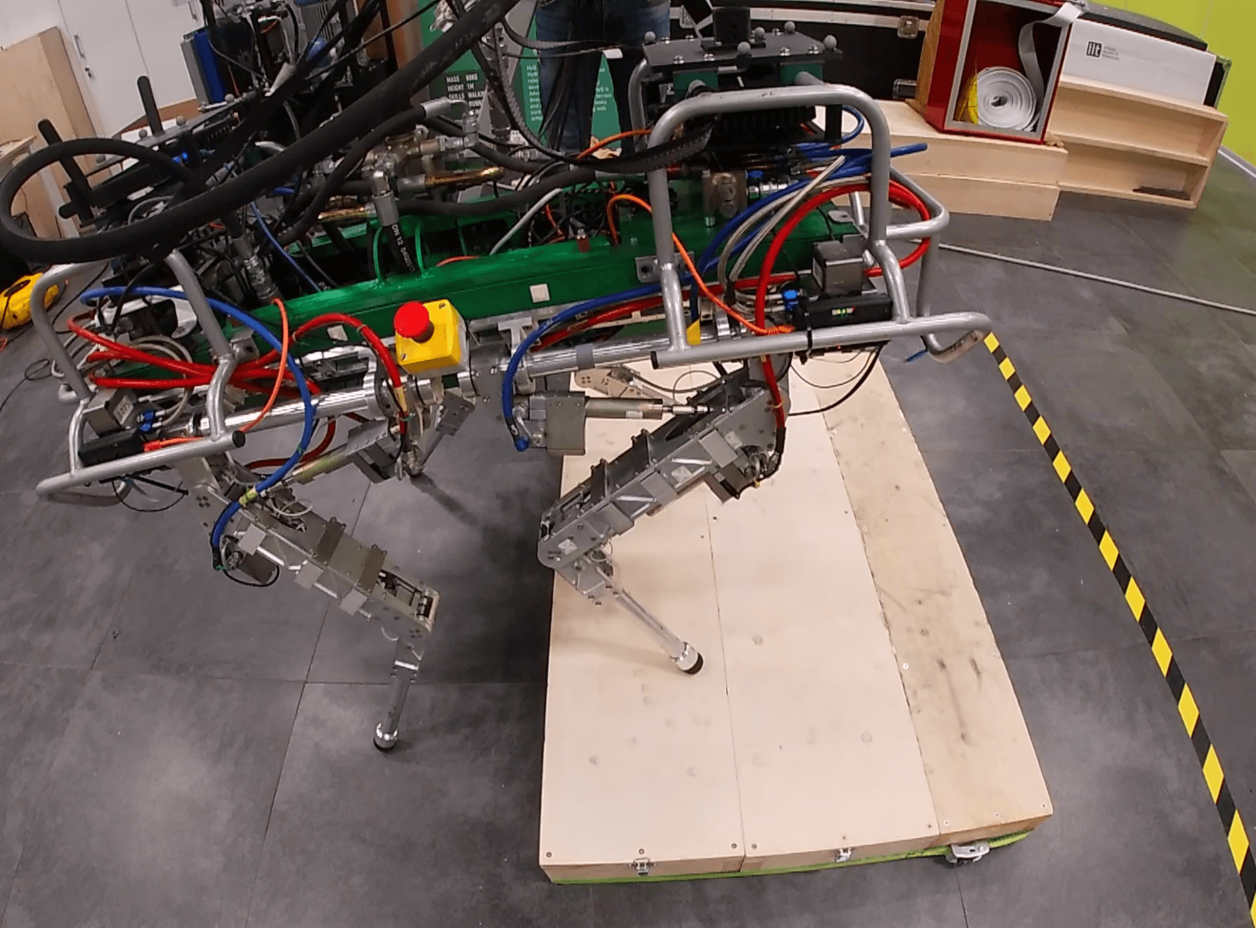
Figure 1: IIT’s quadruped robot HyQ traversing a pallet with the mobility enhanced real-time NMPC.

I Introduction

The main advantage of legged robots with respect to their wheeled counterpart is their ability to traverse complex and unstructured environment such as forests, obstacles, and debris. However, the control of legged robots poses complex problems related to underactuation (the body is controlled only indirectly through the legs), and to the hybrid nature of the forces required to generate motion, since the robot needs to establish and interrupt contact between its feet and the ground. The control design for legged robots was initially dealt with by using heuristic approaches which yielded successful results such as in the walking machines from Raibert [1], the virtual model control of Pratt et al. [2] and in the heuristic locomotion planning for quadrupedal robots by Focchi et al. [3]. However, heuristic approaches have several limitations, for example: 1) they cannot be easily generalized to all kinds of terrain and motions; 2) they cannot account for the future state of the robot hence, they have no possibility to guarantee physical feasibility of the planned trajectories. The challenge of avoiding these undesirable myopic behaviors in heuristic planning approaches has motivated the research towards new optimization-based predictive locomotion planning.

Formulating the locomotion planning as an optimization problem allows one to represent high-level locomotion tasks as cost functions and system dynamics using constraints. Besides robot dynamics, the locomotion tasks should also respect the contact dynamics such as unilateral force and friction cone constraints, that are critical to stabilize the locomotion. The use of optimization techniques to design Whole-Body Control (WBC) has enabled legged robots to traverse soft terrains [4] and to be versatile in terms of type of gait and motions that a legged robot can achieve [5]. The aforementioned examples are based on the solution of a Quadratic Program that only considers the instantaneous [6] effects of the joint torques on the robot’s base. Further, similar to heuristic approaches mentioned earlier, these approaches do not consider the information about the future states of the robot and hence cannot assure recursive feasiblity.

In order to address this issue, several approaches make use of Trajectory Optimization (TO)-based locomotion planning considering the full dynamics of the robot [7, 8]. However, these approaches usually suffer from high computational time hence they are often restricted to offline (open-loop) use. In general, offline planners [9, 10] neither adapt to quick terrain changes nor cope with state drifts and uncertainties. To address this issue the concept of online re-planning can be used. Online re-planning can intrinsically cope with the problem of error accumulation in planned motion that is common in real scenarios.

For online re-planning, MPC has gained broad interest in the robotics community for legged locomotion. Moreover, the intrinsic feedback mechanism offered by MPC can compensate for modeling errors and disturbances acting on the system provided that the MPC is executed at a sufficiently high rate in closed-loop. A careful choice of the dynamic model inside MPC formulation is typically required to achieve a desired re-planning frequency in closed-loop, given the limited computational resources available for online computations. For example, using a full dynamics model of legged robots inside MPC [11, 12] with long prediction horizon may result in an optimization problem which requires excessive computations for real-time deployment at high sampling rates. Using approximate models is a way to reduce the complexity of the optimization, trading the accuracy with computational efficiency. Following this line, [13] used a Centroidal Dynamics (CD) plus a full-kinematic model to enforce the kinematic limits in TO to plan complex behaviors on the humanoid robot Atlas. The CD model considers contact forces as input and links the linear and angular momentum of the robot to the external wrench [14].

A simplified version of the CD model is the Single Rigid Body Dynamics (SRBD) model where the inertia of the legs is neglected (assumption of massless legs) and the robot’s body and legs are lumped into a single rigid body. This model is well suited for quadrupeds, since they usually concentrate their mass and inertia in the robot base, unlike humanoids. The SRBD model was used for TO [15] and MPC [16] to jointly optimize for footholds, Center of Mass (CoM) trajectories and contact forces. By further linearizing the angular part of the dynamics of the SRBD, [17] was able to achieve a variety of quadrupedal gaits in experiments but their approach was not suitable for motions that involve large variations from the horizontal orientation. The simplest among all the approximate models mentioned earlier is the Linear Inverted Pendulum Model (LIPM) and it has been used inside MPC for quadruped [18] and biped [19] locomotion. However, there are two main limitations in LIPM, namely it neglects angular dynamics and assumes constant robot height. Additionally, it does not account for friction cones, so that the contact stability on non-flat terrain can not be guaranteed.

While models play an important role in obtaining computationally light MPC formulations, the choice of solution method is also paramount to achieve fast online re-planning with MPC. A Differential Dynamic Programming (DDP) based approach demonstrated the real-time performance with whole-body MPC [12] on HRP-2 humanoid. Recently, [20] proposed a DDP-based MPC using a kinodynamic model which re-plans at a frequency of $15\,\mathrm{Hz}$ with a prediction horizon of $1\,\mathrm{s}$ on a quadruped. The main drawbacks of DDP based approaches is the difficulty in implementing hard-inequality and switching constraints. Hard-inequality constraints need to be implemented as penalties (e.g., with relaxed-barriers) [21] while the switching constraints are formulated using Augmented Lagrangian methods [22, 23]. Though not obvious at first sight, these methods are essentially equivalent to direct optimal control based on multiple-shooting [24] in combination with some form of Nonlinear Programming (NLP) solvers using barrier functions in the real-time iteration scheme [25]. One such framework is provided by acados [26].

In addition to DDP-based MPC, there also exist a few implementations of NLP-based MPC for legged robots. One such NMPC implementation with CoM dynamics plus full kinematic model was demonstrated in [27] using a Sequential Linear Quadratic (SLQ) algorithm for a trotting gait on flat terrain. Neunert et al. [11] achieved a fast re-planning frequency of $80$-$170~{}\mathrm{Hz}$ for a small prediction horizon of $0.5~{}\mathrm{s}$ ($125$ nodes) with their NMPC using the full dynamics of the robot, and optimizing foot locations, swing timing, and locomotion sequences along with full body dynamics. However, in the real experiments they have only demonstrated slow trotting on flat terrain. Moreover, since their approach does not consider the map of the terrain, it has limited application on uneven terrain conditions. An interesting observation is that they did not see a noticeable degradation in the closed-loop performance of the NMPC when the re-planning frequency was dropped until 30 $\mathrm{Hz}$, demonstrating that the predictive nature of the MPC empowers the robot to tolerate much lower re-planning frequency. A similar observation was made in [28] with an MPC scheme which optimizes foot locations, but requires a heuristic conditioning of the cost function. In their experiments, the robot is stable if the re-planning occurs at $20\ \mathrm{Hz}$, unstable for lower frequencies and the performance improvement is observed over $40\ \mathrm{Hz}$.

The aforementioned approaches have been successful in controlling legged robots, but neglected an important aspect of these robots, which is usually referred to as mobility. In this paper, we define the mobility as the attitude of the robot leg to arbitrarily change its foot position [29]. We noticed that maximizing mobility improves terrain adaptation hence it is advantageous to account for it in the motion planning of legged robots. Furthermore, as discussed in Section IV-A, adding mobility in the NMPC cost eliminates the need to specify references for the roll, pitch and height of the robot.

To achieve kinematically suitable configurations for the legs, a common heuristic is to align the robot base with the terrain inclination (estimated in [3] via fitting an averaging plane through the stance feet). This approach aims to bring the legs as close as possible to the middle of their workspaces in order to avoid the violation of the kinematic limits. Optimization of mobility allows to achieve a similar behaviour in an automatic way. Fankhauser et al. in [30] maximized mobility by encoding it in a cost function that penalizes the distance with respect to a default foot position. Recently, Cebe et al. [31] implemented TO using an SRBD model and also incorporating the feet positions in the optimization. They re-plan only at the feet touchdowns due to the high computation demand of their TO algorithm and showed experimental results on uneven terrain. Since their planner does not plan during the swing phase of the legs, they do not run their planner in an MPC fashion. Apart from the previously mentioned contributions, to the best of our knowledge no prior work has addressed the mobility with MPC in legged locomotion.

I-A Proposed Approach and Contribution

In this work, we demonstrate in experiments with our $87\,\mathrm{kg}$ Hydraulically actuated Quadruped (HyQ) robot [32] that a suitably formulated NMPC can tackle rough terrain locomotion, account for leg mobility, and provide the optimal base orientation, while being real-time feasible. Indeed, optimizing for leg mobility allows our NMPC to devise a robot base orientation and height that improves locomotion on rough terrain.

This is particularly useful to achieve environment adaptation on rough terrains. Another advantage is that minimal heuristics is required from the user i.e., no reference trajectory for the robot’s height, and its base roll and pitch orientation is needed.

This work is a system integration on the same line of our previous work [33]. However, while in [33] only offline optimization was performed, here we achieve real-time feasible online replanning in an MPC fashion. To achieve this goal:

1. We consider a simplified SRBD model that describes the angular and translational dynamics of the robot base but neglects the dynamics of legs.

2. We employ the real-time iteration (RTI) scheme [25, 34, 35] that allows us to run our NMPC online with the prediction horizon of $2\,\mathrm{s}$ (50 nodes) as opposed to the $0.5\,\mathrm{s}$ ($125$ nodes) used by [11]. Differently from [31] (that re-plans at each foot touchdown event), we continuously re-plan at the rate of $25\,\mathrm{Hz}$.

3. We run our NMPC on a single computer along with the rest of our locomotion framework unlike in [31, 11] where they use dedicated computers for their TO and NMPC, respectively.

We show in simulation the robot traversing a set of pallets of different dimensions placed relatively at varying distances, walking into a V-shaped chimney and lastly over a randomly generated rough terrain. We present Experimental results that demonstrate the capability of our NMPC to generate an omni-directional walk and to traverse a pallet for our quadruped robot HyQ (see Fig. 1). We tested the re-planning capability of our approach by pushing a pallet in front of the robot while walking, such that the control algorithm has to re-plan online in order to adapt to a dynamically changing environment.

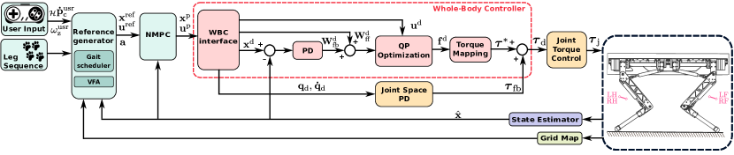
Figure 2: Block diagram of the planning pipeline with the NMPC in our locomotion framework. The reference generator provides the references ($\mathbf{x}^{\mathrm{ref}}$, $\mathbf{u}^{\mathrm{ref}}$) to NMPC after receiving the user inputs. Then the NMPC passes optimal state $\mathbf{x}^{\mathrm{p}}$ and control $\mathbf{x}^{\mathrm{p}}$ trajectories to the Whole-Body Controller. The torque $\bm{\tau}_{\mathrm{d}}$ is given as reference to low level joint torque controller. The state estimator provides the state estimation $\mathbf{\hat{x}}$ to the required blocks. Finally, the heightmap is generated by Grid Map and given to the reference generator.

To summarize, the contributions of our work (in order of importance) are as follows:

• Major experimental results are presented in Section VIII where we demonstrate the capability of our NMPC planner to generate an omni-directional walk and rough terrain locomotion for our quadruped robot HyQ, by exploiting an online evaluation of the map of the terrain and using on-board state estimation.

• Additional (minor) contributions are:

  1. We introduce a cost term which accounts for mobility by penalizing hip-to-foot positions that do not provide the highest mobility. To the best of our knowledge, this is the first time that mobility has been addressed with MPC.

  2. The generation of the reference trajectory for the NMPC takes into account premature and delayed touchdown of the feet as well as continuously adjusting the footholds according to the robot body motion and the terrain features.

  3. We use a parametric robot model that results in smaller NMPC formulation.

I-B Outline

The paper is organized as follows: Section II gives an overview of our planning pipeline whereas Section III describes the NMPC setup. The leg mobility and other features are explained in Section IV, whereas the generation of the references and the WBC are detailed in Sections V and VI, respectively. We then summarize the RTI scheme for our NMPC in Section VII. Further, Section VIII illustrates simulation and experimental results with the HyQ robot. Finally, we draw the conclusions in Section IX.

II Locomotion Framework

Fig. 2 illustrates the planning pipeline of our locomotion framework. The reference generator, as discussed in Section V, takes the user input (longitudinal, lateral and angular velocity), schedule of the gait (e.g., a crawl) timing, the initial state of the robot, and a map of the terrain to generate reference trajectories for the state $\mathbf{x}^{\mathrm{ref}}$ and control input $\mathbf{u}^{\mathrm{ref}}$ required by the NMPC. The reference generator also provides a vector of parameters $\mathbf{a}$ to the NMPC, that includes foot locations and sequences of contact status. The NMPC running at $25\,\mathrm{Hz}$, delivers the optimal trajectories of the state $\mathbf{x}^{\mathrm{p}}$ and control input $\mathbf{u}^{\mathrm{p}}$, as detailed in Section III.

All the components of the Whole-Body controller (highlighted with dashed box in Fig. 2) are discussed in Section VI. The WBC interface interpolates the optimal state $\mathbf{x}^{\mathrm{p}}$ at a rate of $250\,\mathrm{Hz}$ to generate a desired signal $\mathbf{x}^{\mathrm{d}}$ for a Cartesian virtual impedance controller [36]. The WBC interface also computes the feedforward wrench $\mathbf{W}^{\mathrm{d}}_{\mathrm{ff}}$ that is added to a feedback wrench $\mathbf{W}^{\mathrm{d}}_{\mathrm{fb}}$ that renders the Cartesian impedance. Moreover, the WBC interface provides the joint position $\mathbf{q}_{\mathrm{d}}$ and velocities $\mathbf{\dot{q}}_{\mathrm{d}}$ to a Joint Space PD controller running at $1\,\mathrm{kHz}$. After acquiring the feedback and feed-forward wrenches, a Quadratic Programming (QP) optimization computes the vector of desired Ground Reaction Forces (GRFs) $\mathbf{f}^{\mathrm{d}}$ accounting for the friction cone constraints and penalizing the the difference between $\mathbf{f}^{\mathrm{d}}$ and $\mathbf{u}^{\mathrm{p}}$ coming from the NMPC solution. Then, $\mathbf{f}^{\mathrm{d}}$ is mapped to the torque vector $\bm{\tau}^{*}$ that is added to the Joint Space PD torques $\bm{\tau}_{\mathrm{fb}}$ resulting into the total desired torque $\bm{\tau}_{\mathrm{d}}$. Ultimately, $\bm{\tau}_{\mathrm{d}}$ is passed to a low-level joint torque controller as reference [37].

An online state estimator [38] that runs at $500\,\mathrm{Hz}$ provides the estimation of the robot state $\mathbf{\hat{x}}$ to all the components inside our locomotion framework that require it. A dedicated on-board computer takes inputs from an RGB-D camera (RealSense) mounted in front of the robot and generates a 2.5D heightmap at the rate of $30\,\mathrm{Hz}$ using the Grid Map library from [39]. This heightmap is later sent to the reference generator.

III NMPC

In our planning algorithm, we choose a real-time NMPC formulation because it has the ability to handle both the nonlinear system dynamics and the constraints, explicitly. NMPC is based on solving an Optimal Control Problem (OCP) given the current state $\mathbf{\hat{x}}_{0}$ of the system. Only the first element of the optimized input trajectory is applied to the system, then the state is measured and the OCP is solved again based on the new state measurement to close the loop.

We define the decision variables as the predicted state and control input with $\mathbf{x}^{\mathrm{p}}=\{\mathbf{x}_{0},\ldots,\mathbf{x}_{N}\}$ and $\mathbf{u}^{\mathrm{p}}=\{\mathbf{u}_{0},\ldots,\mathbf{u}_{N-1}\}$, respectively, such that an NLP formulation can be stated as:

$$\displaystyle{\min_{\mathbf{x}^{\mathrm{p}},\mathbf{u}^{\mathrm{p}}}}\quad \sum_{k=0}^{N-1}\ell\left(\mathbf{x}_{k},\mathbf{u}_{k},\mathbf{a}_{k}\right)+\ell_{\mathrm{T}}\left(\mathbf{x}_{N}\right)$$ (1a)

s.t. $$\mathbf{x}_{0}=\bm{\hat{\mathbf{x}}_{0}},$$ (1b)

$$\mathbf{x}_{k+1}=f\left(\mathbf{x}_{k},\mathbf{u}_{k},\mathbf{a}_{k}\right), k\in\mathbb{I}_{0}^{N-1},$$ (1c)

$$h\left(\mathbf{x}_{k},\mathbf{u}_{k},\mathbf{a}_{k}\right)\leq 0, k\in\mathbb{I}_{0}^{N-1},$$ (1d)

where, $\ell:\mathbb{R}^{n_{x}}\times\mathbb{R}^{n_{u}}\times\mathbb{R}^{n_{a}}\rightarrow\mathbb{R}$ is the stage cost function; $\ell_{\mathrm{T}}:\mathbb{R}^{n_{x}}\rightarrow\mathbb{R}$ is the terminal cost function. The initial condition (1b) is expressed by setting $\mathbf{x}_{0}$ equal to the state estimate $\bm{\hat{\mathbf{x}}_{0}}$ received from the state estimator. The vector of model parameters $\mathbf{a}_{k}$ is not optimized but it is computed externally by the reference generator and provided to the optimization problem formulation. The nonlinear system dynamics are introduced by the equality constraints (1c). Finally, the path constraints are included with (1d) which, for example, can be bounds on the decision variables. The NLP (1) is defined for a prediction horizon $T$ that is divided into $N$ discrete time control intervals of lengths $T_{\mathrm{s}}=\frac{T}{N}$. Hereafter, we will refer to $T_{\mathrm{s}}$ as the sampling time.

III-A Cost

In our NMPC formulation we use a cost function of the form:

$$\ell\left(\mathbf{x}_{k},\mathbf{u}_{k},\mathbf{a}_{k}\right)= \,\ell_{\mathrm{t}}+\ell_{\mathrm{m}}+\ell_{\mathrm{r}},$$ (2a)

$$\ell_{\mathrm{t}}= \parallel\mathbf{x}_{k}-\mathbf{x}^{\mathrm{ref}}_{k}\parallel_{\mathbf{\bm{Q}}}^{2}+\parallel\mathbf{u}_{k}-\mathbf{u}^{\mathrm{ref}}_{k}\parallel_{\mathbf{\bm{R}}}^{2},$$ (2b)

$$\ell_{\mathrm{m}}= \parallel{}_{\mathcal{C}}\mathbf{p}_{\mathrm{hf}_{k}}-{}_{\mathcal{C}}\mathbf{p}_{\mathrm{hf}_{k}}^{\mathrm{ref}}\parallel_{\mathbf{\bm{M}}}^{2},$$ (2c)

$$\ell_{\mathrm{r}}= \,\rho\parallel{{}_{\mathcal{K}}\mathbf{u}_{k}}\parallel_{\mathbf{\bm{P}}}^{2}$$ (2d)

• The tracking cost (2b) is associated to state and control input and the references trajectories $\mathbf{x}^{\mathrm{ref}}_{k},\mathbf{u}^{\mathrm{ref}}_{k}$ are provided by the reference generator for each sampling instance $k$ (refer Section V).

• The mobility cost (2c) is one of the contributions of this work that accounts for improving the leg mobility by penalizing the difference between the hip-to-foot distance ${}_{\mathcal{C}}\mathbf{p}_{\mathrm{hf}}$ and the reference value ${}_{\mathcal{C}}\mathbf{p}_{\mathrm{hf}}^{\mathrm{ref}}$ of maximum mobility. This cost allows the NMPC to optimize the robot base orientation (e.g. align it to the terrain shape) in order to increase the leg mobility which has as a desirable consequence to stay far from kinematic limits during locomotion. The derivation of ${}_{\mathcal{C}}\mathbf{p}_{\mathrm{hf}}^{\mathrm{ref}}$ is detailed separately in Section IV-A.

• In some locomotion scenarios [36], to cope with uncertainties in the contact normal estimation and increase robustness to external disturbances, it is desirable to have the GRFs $\mathbf{f}_{i}$ as close as possible to the center of the friction cone. This can be achieved with by penalizing $X$-$Y$ components of $\mathbf{u}$ in a frame $\mathcal{K}$ (see Fig. 3) that is aligned to the normal of the contact and it is included in our cost function by a control input regularization term (2d), refer Section IV-C for the details.

The positive definite weight matrices $\mathbf{\bm{Q}}\in\mathbb{S}_{+}^{n_{x}},\mathbf{\bm{R}}\in\mathbb{S}_{+}^{n_{u}}$, $\mathbf{\bm{M}}\in\mathbb{S}_{+}^{12}$, $\mathbf{\bm{P}}\in\mathbb{S}_{+}^{n_{u}}$ act as important tuning parameters in the NMPC formulation. The regularization factor $\rho$ decides the trade-off between force robustness cost (2d) and both the tracking (2b) and mobility (2c) cost. Finally, we define the terminal cost $\ell_{\mathrm{T}}=\parallel\mathbf{x}_{N}-\mathbf{x}^{\mathrm{ref}}_{N}\parallel_{\mathbf{\bm{Q}}_{N}}$ and use the weight matrix ${\mathbf{\bm{Q}}_{N}}={\mathbf{\bm{Q}}}$ for this cost.

III-B Robot Model

The inertial frame $\mathcal{W}$ and the CoM frame $\mathcal{C}$ are shown in Fig. 3. The CoM frame is aligned with the base of the robot and its origin is located at the CoM. A variable with left subscript denotes its frame of reference. For example ${}_{\mathcal{C}}\bm{\omega}$ represents the angular velocity of the robot base expressed in the CoM frame $\mathcal{C}$. Note that, unless explicitly specified, all the relevant quantities in this paper are defined in the inertial frame $\mathcal{W}$. Throughout this paper we define $(a,\ldots,b)$ as the column vector stacking any generic column vectors $a,\ldots,b$.

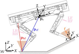
Figure 3: HyQ schematic showing the inertial frame ($\mathcal{W}$), the CoM frame ($\mathcal{C}$) attached to the CoM of the robot, and the contact frame ($\mathcal{K}$). The robot legs are shown in the default configuration.

We use a simplified reduced-order SRBD model [15] defined in a 6D space that describes the translational and angular dynamics of the robot while neglecting the dynamics of its swinging legs. This is a valid approximation for the HyQ robot because most of its mass is concentrated in the base, as mentioned in [32] (the mass of the base is $61\,\mathrm{kg}$ and the mass of each leg is $6.5\,\mathrm{kg}$). The robot is approximated as a rigid body with the inertia computed considering the robot in a default leg configuration as shown in Fig. 3. We choose to define the SRBD model in the CoM frame (specifically the angular dynamics) because this choice yields a constant inertia tensor. Thus, the angular dynamic equations are much simpler i.e., less non-linear because the inertia tensor is not time varying. In the SRBD model, GRFs are applied as inputs to control the position and orientation of the robot base. The SRBD model is:

$$m\dot{\mathbf{v}}_{\mathrm{c}} =m\mathbf{g}+\sum_{i=1}^{4}\delta_{i}\mathbf{f}_{i}$$ (3a)

$${}_{\mathcal{C}}\mathbf{\bm{I}}_{\mathrm{c}}\,{}_{\mathcal{C}}\dot{\bm{\omega}}+{}_{\mathcal{C}}\bm{\omega}\times{}_{\mathcal{C}}\mathbf{\bm{I}}_{\mathrm{c}}{}_{\mathcal{C}}\bm{\omega} =\sum_{i=1}^{4}\delta_{i}{}_{\mathcal{C}}\mathbf{p}_{\mathrm{cf},i}\times{}_{\mathcal{C}}\mathbf{f}_{i}$$ (3b)

where $m$ is the robot mass, $\dot{\mathbf{v}}_{\mathrm{c}}\in\mathbb{R}^{3}$ is the CoM acceleration, $\mathbf{g}$ is the gravitational acceleration, $\mathbf{f}_{i}\in\mathbb{R}^{3}$ is the ground reaction force at foot $i$, ${}_{\mathcal{C}}\mathbf{\bm{I}}_{\mathrm{c}}\in\mathbb{R}^{3\times 3}$ is the inertia tensor computed at the CoM frame origin, ${}_{\mathcal{C}}\dot{\bm{\omega}}\in\mathbb{R}^{3}$ is the angular acceleration of the robot’s base, $\mathbf{p}_{\mathrm{cf},i}\in\mathbb{R}^{3}$ is the distance between the CoM position $\mathbf{p}_{\mathrm{c}}\in\mathbb{R}^{3}$ and the position $\mathbf{p}_{\mathrm{f},i}\in\mathbb{R}^{3}$ of foot $i$. We introduce binary parameters $\delta_{i}=\{0,1\}$ to define whether foot $i$ is in contact with the ground and can therefore generate contact forces or not.

The robot dynamics governed by (3) can be expressed as the continuous-time state-space model:

$$\begin{bmatrix}\dot{\mathbf{p}}_{\mathrm{c}}\\ \dot{\mathbf{v}}_{\mathrm{c}}\\ \dot{\bm{\Phi}}\\ {}_{\mathcal{C}}\dot{\bm{\omega}}\end{bmatrix}=\begin{bmatrix}{\mathbf{v}}_{\mathrm{c}}\\ 1/m\sum_{i=1}^{4}\delta_{i}\mathbf{f}_{i}+\mathbf{g}\\ \mathbf{\bm{E}}^{\prime-1}(\bm{\Phi}){}_{\mathcal{C}}\bm{\omega}\\ -{}_{\mathcal{C}}\mathbf{\bm{I}}^{-1}_{\mathrm{c}}({}_{\mathcal{C}}\bm{\omega}\times{}_{\mathcal{C}}\mathbf{\bm{I}}_{\mathrm{c}}){}_{\mathcal{C}}\bm{\omega}+\sum_{i=1}^{4}\delta_{i}{}_{\mathcal{C}}\mathbf{\bm{I}}^{-1}_{\mathrm{c}}{}_{\mathcal{C}}\mathbf{p}_{\mathrm{cf},i}\times{}_{\mathcal{C}}\mathbf{f}_{i}\end{bmatrix}$$ (4)

where $\mathbf{v}_{\mathrm{c}}$ is the CoM velocity of the robot. The robot base orientation is represented by the sequence of $Z$-$Y$-$X$ Euler angles [41] $\bm{\Phi}=(\phi,\,\theta,\,\psi)$ i.e., roll ($\phi$), pitch ($\theta$) and yaw ($\psi$), respectively. The relation between the Euler Angles rates $\dot{\bm{\Phi}}$ and angular velocity ${}_{\mathcal{C}}\bm{\omega}$ is well-known and discussed in Appendix A for the sake of completeness. We define the state and control vectors as $\mathbf{x}=(\mathbf{p}_{\mathrm{c}},\,\mathbf{v}_{\mathrm{c}},\,\bm{\Phi},\,{}_{\mathcal{C}}\bm{\omega})$, and $\mathbf{u}=(\mathbf{f}_{1},\ldots,\mathbf{f}_{4})$. Equation (4) can be concisely written as:

$$\dot{\mathbf{x}}(t)=g(\mathbf{x}(t),\mathbf{u}(t),\mathbf{a}(t)),$$ (5)

where $\mathbf{a}=(\mathbf{p}_{\mathrm{f}},\,\bm{\delta})$ is a vector of parameters that includes the feet positions $\mathbf{p}_{\mathrm{f}}$ and the contact status $\bm{\delta}\in\mathbb{R}^{4}$.

The rigid-body dynamics (5) are discretized using numerical integration [42, 43, 44, 45] to obtain the discrete-time model:

$$\mathbf{x}_{k+1}=f\left(\mathbf{x}_{k},\mathbf{u}_{k},\mathbf{a}_{k}\right),$$ (6)

which defines equality constraints (1c) imposed at every stage $k$ in MPC to ensure that the state trajectory satisfies the system dynamics for the given control inputs.

One specific feature of legged robots is the need to ensure that the values of the GRFs equal to zero for a swinging leg. This is typically done by introducing complementarity constraints [31, 46]. These constraints, however, pose several difficulties in the solution of the optimization problem, since the vast majority of the NLP algorithms cannot handle them and tailored solvers are required. Ultimately, this results in a significant increase in computation time. An alternative to complementarity constraints consists in providing the sequence of contact status $\bm{\delta}$ as input parameters in the state space model (5). In this manner, a contact mode $\delta_{i}$ is multiplied with the terms involving force $\mathbf{f}_{i}$ in (4) and the contribution of that force is nullified during the swing phase of the corresponding leg $i$. Hence, there is no more need to include complementarity constraints separately in (1) which results in fewer constraints and, consequently, in a relatively smaller NMPC formulation.

III-C Friction cone and unilateral constraints

Friction cone constraints are encoded with their square pyramid approximation:

$$-\mu_{i}\mathbf{f}_{\mathrm{z},i} \leq\mathbf{f}_{\mathrm{x},i}\leq\mu_{i}\mathbf{f}_{\mathrm{z},i}$$ (7a)

$$-\mu_{i}\mathbf{f}_{\mathrm{z},i} \leq\mathbf{f}_{\mathrm{y},i}\leq\mu_{i}\mathbf{f}_{\mathrm{z},i}$$ (7b)

$$\underline{\mathbf{f}}_{\mathrm{z}} \leq\mathbf{f}_{\mathrm{z},i}\leq\overline{\mathbf{f}}_{\mathrm{z}}$$ (7c)

where, $\underline{\mathbf{f}}_{\mathrm{z}}$ and $\overline{\mathbf{f}}_{\mathrm{z}}$ are upper and lower bounds on GRFs $Z$ component, respectively, and $\mu_{i}$ is the friction coefficient of the contact surface. Choosing $\underline{\mathbf{f}}_{z}$ greater than or equal to zero enforces unilateral constraints on the normal forces $\mathbf{f}_{\mathrm{z}}$. The friction cone and unilateral constraint are represented by $h\left(\mathbf{x}_{k},\mathbf{u}_{k},\mathbf{a}_{k}\right)\leq 0$ in the NMPC formulation.

IV Locomotion-Enhancing Features

In this section we discuss the main distinctive features of our approach, which we found relevant to improve locomotion ability of our quadruped robot. These features are mobility, force robustness and Zero Moment Point (ZMP) margin.

IV-A Mobility and Mobility Factor

Terrain adaptability is vital when it comes to locomotion of the legged robots. Adjusting the posture of the robot depending on the environment is important for safe locomotion. A way to enable our NMPC to choose robot orientation adaptively to any terrain is to employ the concept of mobility [47]. In order to rigorously discuss mobility in mathematical terms, we first define it in words as the attitude of a manipulator (leg) to arbitrarily change end-effector position/orientation [29].

In order to penalize low leg mobility in the cost function (2c) we need to compute the reference value of hip-to-foot distance ${}_{\mathcal{C}}\mathbf{p}_{\mathrm{hf}_{k}}^{\mathrm{ref}}$. Our goal in this section is to define a convenient metric to represent mobility and compute ${}_{\mathcal{C}}\mathbf{p}_{\mathrm{hf}_{k}}^{\mathrm{ref}}$ corresponding to the maximum value of such a metric. Among several ways to compute mobility [47], the velocity transformation ratio [48] allows one to evaluate mobility in a particular direction. However, the velocity transformation ratio cannot be used in our setting because it requires prior knowledge of the evolution of the relative foot position with respect to CoM. In our case it is not available in advance because it is an output the NMPC.

As an alternative approach, we consider the volume of the manipulability ellipsoid $\left(\mathbf{v}(\mathbf{\bm{J}}\mathbf{\bm{J}}^{\top})^{-1}\mathbf{v}=1\right)$ [29] as a metric to evaluate mobility. A change in the volume of the manipulability ellipsoid with different leg configurations is visualized in Fig. 4 (left).

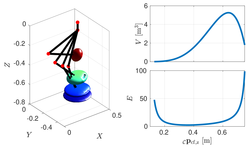
Figure 4: Manipulability ellipsoid changing with leg configuration (left) of the right front leg. Volume of the ellipsoid (top right) and Eccentricity of the ellipsoid (bottom right).

Inspecting Fig. 4 (top right), it can be seen that the maximum volume $V$ is in the vicinity of the most extended leg configuration because the mobility becomes very big in the $X$ and $Y$ direction, even if it is still very limited in the $Z$ direction. However, because it is desirable to achieve a good mobility in all the directions of the leg configuration, a better metric to do so is the one that accounts for the isotropy of the manipulability ellipsoid. A measure of the isotropy of an ellipsoid can be expressed as the inverse of its eccentricity $E$. Hence, a new manipulability index that we call mobility factor (8) can be defined in terms of both the eccentricity and the volume of manipulability ellipsoid. Again from Fig. 4, it can be visualized that to keep a good mobility (left plot) in all directions, the volume (top right plot) should be maximized while the eccentricity (bottom right plot) as small as possible. Defining a foot Jacobian $\mathbf{\bm{J}}(\mathbf{q})\in\mathbb{R}^{3\times 3}$ computed at a particular joint configuration $\mathbf{q}$, the volume $V$ of a manipulability ellipsoid is evaluated as a product of the eigenvalues of $\left(\mathbf{\bm{J}}(\mathbf{q})\mathbf{\bm{J}}(\mathbf{q})^{\top}\right)^{-1}$ while the eccentricity is the ratio between its maximum and minimum eigenvalue [47]. First, the volume and eccentricity of manipulability ellipsoid are normalized by their ranges $\bar{V}$ and $\bar{E}$. Then we define the mobility factor as:

$$m_{\mathrm{f}}=\beta\frac{V}{\bar{V}}-\gamma\frac{E}{\bar{E}}$$ (8)

The minus sign in (8) represents conflicting contributions of the $V$ and $E$ in the definition of the mobility factor (i.e. the goal is to achieve high volume and low eccentricity). Parameters $\beta$ and $\gamma$ are introduced to find a best trade-off between volume and eccentricity while deciding a mobility factor.

The mobility factor is a convex nonlinear function $m_{\mathrm{f}}:\mathbb{R}^{3}\to\mathbb{R}$ that can be numerically evaluated inside the workspace of each leg. By selecting $\beta=1$ and $\gamma=4$, and after conducting a numerical analysis for all the feet positions in the workspace of a leg of the HyQ robot we found that hip-to-foot distance ${}_{\mathcal{C}}\mathbf{p}_{\mathrm{hf}}=(0,0,-0.55)\,\mathrm{m}$ maximizes $m_{\mathrm{f}}$. In Fig. 5 (left) we show a slice of the scalar function $m_{\mathrm{f}}$ in the $X$-$Y$ plane for ${}_{\mathcal{C}}\mathbf{p}_{\mathrm{hf,z}}=-0.55\,\mathrm{m}$ obtained for the Right-Front (RF) leg. Instead, in Fig. 5 (right) we plot $m_{\mathrm{f}}$ against the change of foot position in the $Z$ direction considering the hip under the foot ($X=0$, $Y=0$) which clearly highlights ${}_{\mathcal{C}}\mathbf{p}_{\mathrm{hf,z}}=-0.55\,\mathrm{m}$ corresponding to the maximum value of the mobility factor $m_{\mathrm{f}}$ (i.e., around 0.41). We use the output of this analysis as a reference for the hip-to-foot distance ${}_{\mathcal{C}}\mathbf{p}_{\mathrm{hf}}^{\mathrm{ref}}$ in the mobility cost (2c) for all the legs.

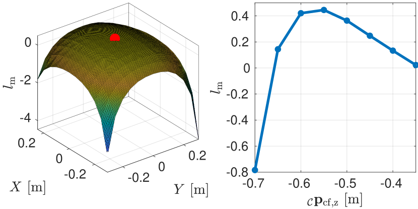
Figure 5: Slices of the mobility factor function for the RF leg: the left figure plots it against the $X$-$Y$ components keeping $Z$ constant. The red dot in the left plot represents the maxima. The right figure plots it against the $Z$ component for a constant $X$-$Y$ foot position.

In the mobility cost, we multiply $\delta_{i}$ to the term corresponding to the $i^{\mathrm{th}}$ leg. Thus, the mobility cost solely accounts for stance legs because the robot can only use them to control its base orientation. Since, including the mobility cost enables NMPC to provide the optimal base orientation for a particular locomotion that retains mobility, there is no need to separately specify tracking cost for roll and pitch in the NMPC. This relieves a user from the burden of implementing a customized heuristic (e.g., to align the robot base to the terrain), as was necessary in, e.g., [3, 49, 46]. The relative tracking task for the CoM $Z$ position is no longer required either, because maximizing the mobility in the $Z$ direction automatically takes care of keeping an average distance of hips from the terrain to ${}_{\mathcal{C}}\mathbf{p}_{\mathrm{hf,z}}$, consequently keeping the robot base at a certain height.

Moreover, the yaw motion results by penalizing the mobility cost along the $X$-$Y$ directions. This has the effect of driving the hips of the robot base over the feet, naturally aligning the base to the feet, similar to what was done in [50]. However, a tracking cost on yaw was still necessary in the NMPC to track the heading velocity $\omega^{\mathrm{usr}}_{\mathrm{z}}$ commanded by the user and to avoid oscillations.

Remark: The concept of mobility is model independent hence, it can also be used with other models such as full body dynamics in the MPC setting.

IV-B ZMP Margin

In legged locomotion, the robot is often operated close to unstable configurations which require a controller to continuously compensate for model inaccuracies and external disturbances while maintaining locomotion stability. However, a configuration in which the ZMP [51] is close to the boundary of the support polygon [52] could cause instability even with small perturbations due to the loss of control authority.

In our case, the reference generator computes references for the GRFs by dividing the robot mass with the number of legs as explained in Section V. Penalizing GRFs $Z$ component heavily in the tracking cost (2b) ensures that they stay close to the reference, consequently maintaining a higher loading on the diagonally opposite leg to the swinging one, and therefore maintaining some margin for the locomotion stability. To evaluate the locomotion stability, we define the ZMP margin which is computed as the minimum of the distance of the ZMP from each support polygon edge, i.e.,

$$m_{\mathrm{c}}=\min(\mathbf{d})$$ (9)

where $\mathbf{d}$ is a vector of the distances of ZMP projection (on a horizontal plane) from the support polygon edges.

IV-C Force Robustness

Similar to the considerations on mobility, in order to effectively compensate for disturbances acting on the system, robustness in the GRFs is required. The closer the GRF is to the friction cone boundary, the less lateral force is available to compensate for perturbations. An approach penalizing GRFs that are in the vicinity of the cone boundaries has been proposed in [36, 4] inside the WBC. These WBC based approaches instantaneously generate GRFs that are as close as possible to the normals of the cones while yielding the prescribed resultant wrench on the robot base. However, WBC does not account for the future state of the robot and hence, it leaves some room for the NMPC to compensate for the contact normal estimation error and recover from external disturbances. Introducing these margins on GRFs from the cone boundaries is especially important in some scenarios, such as the one reported in simulation in Section VIII-B2.

In this paper, we adopt a similar idea to [36, 4] and introduce the additional cost term (2d) in the NMPC, which penalizes the tangential components of GRFs in the contact frame $\mathcal{K}$ (see Fig. 3) to obtain the resultant GRFs as close as possible to the contact normals. The weight matrix $\mathbf{\bm{P}}$ used in this cost is defined in Table II (Section VIII). Note that it is required to penalize the $X$-$Y$ components higher than $Z$ component of GRFs in the contact frame to achieve this behaviour.

V Reference Generator

In our approach, the NMPC requires a reference trajectory of the state and control input along with the model parameters i.e., foot positions and contact status. For the very first run of the NMPC, this reference trajectory also serves as an initial guess. The references are generated for the length of control intervals $N$, since the reference generator is called before every iteration of the NMPC in order to obtain prompt adaptation to terrain changes and user set-point. Our reference generator is based on heuristics and it takes as inputs:

• the user commanded longitudinal and lateral CoM velocity ${}_{\mathcal{H}}\mathbf{v}_{\mathrm{c}}^{\mathrm{usr}}\in\mathbb{R}^{2}$ in the horizontal frame $\mathcal{H}$,

• user commanded heading velocity $\omega^{\mathrm{usr}}_{\mathrm{z}}\in\mathbb{R}$,

• current pose of the robot $(\mathbf{p}_{\mathrm{c}},\bm{\Phi})$,

• current feet positions $\mathbf{p}_{\mathrm{f}}\in\mathbb{R}^{12}$,

• heightmap of the terrain

The reference generator outputs:

• the references for the NMPC cost: states $\mathbf{x}^{\mathrm{ref}}\in\mathbb{R}^{n_{x}\times(N+1)}$, control $\mathbf{u}^{\mathrm{ref}}\in\mathbb{R}^{n_{u}\times N}$,

• parameters $\mathbf{a}$ of the model: sequence of the contact status $\bm{\delta}$ ($\in\mathbb{R}^{4\times N}$) and sequence of the foot locations $\mathbf{p}_{\mathrm{f}}$ ($\in\mathbb{R}^{12\times N}$),

• normals of the terrain at the foothold locations, which are provided as inputs to the NMPC for the cone constraints.

First we compute the $X$-$Y$ components of the total velocity $\mathbf{v}^{\mathrm{ref}}_{\mathrm{c}}\in\mathbb{R}^{3}$, which depend on both $\mathbf{v}_{\mathrm{c}}^{\mathrm{usr}}$ and the $X$-$Y$ components of the tangential velocity due to the heading velocity $\bm{\omega}^{\mathrm{usr}}$ = $(0,0,\omega^{\mathrm{usr}}_{\mathrm{z}})$.

$$\mathbf{v}^{\mathrm{ref}}_{\mathrm{c,(x,y)}}=\mathbf{v}_{\mathrm{c}}^{\mathrm{usr}}+(\bm{\omega}^{\mathrm{usr}}\times\mathbf{p}_{\mathrm{c}}^{\mathrm{ref}})_{\mathrm{(x,y)}}$$ (10)

The $X$-$Y$ CoM position $\mathbf{p}^{\mathrm{ref}}_{\mathrm{c,(x,y)}}$ is obtained by integrating the $\mathbf{v}^{\mathrm{ref}}_{\mathrm{c,(x,y)}}$ with the explicit Euler scheme. The references for CoM $Z$, roll and pitch are set to $0$ because we do not track them in the NMPC cost (2b). Instead, the reference for the yaw $\psi$ is obtained by integrating the user defined yaw rate $\dot{\psi}^{\mathrm{usr}}$ with $\dot{\bm{\Phi}}^{\mathrm{usr}}=\mathbf{E}^{-1}(\bm{\Phi}^{\mathrm{ref}})\bm{\omega}^{\mathrm{usr}}$ (see Appendix A for the transformation between angular velocity and Euler rates). The reference for angular velocity, instead, coincides with $\bm{\omega}^{\mathrm{usr}}$.
The references for GRFs $\mathbf{u}^{\mathrm{ref}}$ are calculated by simply dividing the total mass of the robot by the number of legs in stance. Dividing the forces equally onto the legs is correct only if the robot is static, but, in case of dynamic conditions, it is a better approximation than passing no references.

The sequence of contact status $\bm{\delta}$ and of footholds are computed by the gait scheduler and robocentric stepping strategy, respectively. It is important to mention that the reference generator does not compute the swing trajectories and they are obtained from the WBC interface discussed in Section VI-A.

V-1 Gait scheduler

The gait scheduler is logically decoupled from the reference trajectory generation and determines if a leg is either in swing or in stance $({\delta}_{i})$ at each time instance for the entire gait cycle as shown in Fig. 6 (left).

The leg duty factor $D_{i}$ and offsets $o_{i}$ can be used to encode different gaits such as crawl, trot and pace. The gait scheduler implements a time parametrization $s\in[0,1]$ (stride phase) which is normalized about the cycle time duration $T_{\mathrm{c}}$ such that the leg duty factor $D_{i}$ and offsets $o_{i}$ are independent from the cycle time. Each trigger $l^{\mathrm{tr}}_{i}$ (red flag in Fig. 6 (left)) corresponds to a new lift-off event. We can express the value of $\delta$ for leg $i$ as:

$$\delta_{i}=\begin{cases}1,&s<o_{i}\vee s>((o_{i}+(1-D_{i}))\bmod 1)\\ 0,&\text{otherwise}\end{cases}$$ (11)

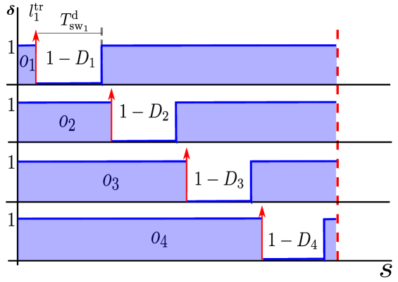
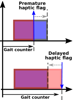
Figure 6: Gait schedule for a walk. Offsets $\mathbf{o}=\left[0.05,0.3,0.55,0.8\right]$, duty-factors $\mathbf{D}=\left[0.85,0.85,0.85,0.85\right]$. The red arrows represent the trigger $l^{\mathrm{tr}}_{i}$ for a swing leg $i$. Right part shows the fast-forwarding (top) or re-winding (bottom) of the gait counter to recover synchronization between actual (haptic) and planned touchdown.

Every time the reference generator is called, it extracts $N$ points from the gait schedule starting from an index called gait counter. It keeps memory of the index of the gait schedule achieved by the previous call of the reference generator. The synchronization between the first point of a contact sequence $\delta_{i_{k}}$ computed by the reference generator and the actual contact state of the robot avoids the reference generator to compute a zero reference force while the leg is in stance and vice-versa. In the case of premature or delayed touchdown events, the synchronization is lost and the gait counter is shifted backwards or forward to re-conciliate the planned touchdown with the actual touchdown as shown in Fig. 6 (right). This is a crucial feature when dealing with rough terrains.

V-2 Robocentric stepping

The choice of the foothold is a key element in locomotion, since it deals with the kinematic limits of the robot. Inspired by [1], we use an approach that continuously computes footholds consistent with the current position of the robot. To compute a foothold for a swinging leg $i$, we consider its hip position $\mathbf{h}_{i}$ instead of using the foot position at the moment of lift-off. In this way a disturbance acting on the robot or a tracking error occurred during a swing can be recovered in the following swing. For a leg $i$, dropping the index to simplify the notation and defining the lift-off trigger as $l^{\mathrm{tr}}_{k}=\delta_{k}\land\overline{\delta}_{k+1}$, the foot position is computed as:

$$\mathbf{p}_{\mathrm{f}_{k+1}}=\begin{cases}\mathbf{p}^{\mathrm{td}}_{\mathrm{f}_{k}}&l^{\mathrm{tr}}_{k}=1\\ \mathbf{p}_{\mathrm{f}_{k}}&l^{\mathrm{tr}}_{k}=0\end{cases}$$ (12)

Notice that at the lift-off condition $l^{\mathrm{tr}}=1$ at instance $k$, $\mathbf{p}_{\mathrm{f}}$ is set equal to the touchdown point $\mathbf{p}^{\mathrm{td}}_{\mathrm{f}}$ and it is kept constant until the next lift-off event occurs. The $X$-$Y$ component of the touchdown point is given by:

$$\mathbf{p}^{\mathrm{td}}_{\mathrm{f}_{k},\mathrm{(x,y)}}=\mathbf{h}_{k}+\alpha T_{\mathrm{sw}}^{\mathrm{d}}(\mathbf{v}_{\mathrm{c}}^{\mathrm{usr}}+(\bm{\omega}^{\mathrm{usr}}\times\mathbf{p}_{\mathrm{bh}})_{\mathrm{(x,y)}})$$ (13)

The second term in (13) represents the step length (red arrow in Fig. 7) which is computed with respect to the hip instead of the previous foot location. Parameter $\alpha$ is an empirically chosen scaling factor. Parameter $T_{\mathrm{sw}}^{\mathrm{d}}$ is the default swing duration computed starting from user-defined offsets $\mathbf{o}$ and duty-factors $\mathbf{D}$. $\mathbf{p}_{\mathrm{bh}}\in\mathbb{R}^{3}$ is the distance between hip and center of the base.

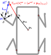
Figure 7: Representation of the robocentric stepping strategy and of the Swing Frame, located at the lift-off point. The red arrow shows the distance between the touchdown point $\mathbf{p}^{\mathrm{td}}_{\mathrm{f}}$ and the hip $\mathbf{h}$. The blue vector $\mathbf{L}_{\mathrm{sw}}$ connects lift-off and touchdown point.

A 2.5D heightmap of the terrain is evaluated in correspondence of the touchdown point $\mathbf{p}^{\mathrm{td}}_{\mathrm{f}_{k},\mathrm{(x,y)}}$, to obtain $\mathbf{p}_{\mathrm{f}_{k},\mathrm{z}}^{\mathrm{td}}$ that does not penetrate the terrain. If $\mathbf{p}_{\mathrm{f}}^{\mathrm{td}}$ is located near an edge or leads to collisions (e.g., of the foot or the shin) during the step cycle, this can be harmful for the robot’s balance. To prevent this from happening, the robot acquires a local heightmap in the vicinity of the touchdown point $\mathbf{p}_{\mathrm{f}}^{\mathrm{td}}$ and adjusts the foot landing location using the Vision-based Foothold Adaptation (VFA) module presented in [53].

VI Whole-Body Controller

In this section, we describe the WBC that tracks planned trajectories $\mathbf{x}^{\mathrm{p}}$ and $\mathbf{u}^{\mathrm{p}}$ provided by the NMPC. The WBC first computes feed-forward $\mathbf{\bm{W}}^{\mathrm{d}}_{\mathrm{ff}}$ and feedback $\mathbf{\bm{W}}^{\mathrm{d}}_{\mathrm{fb}}$ wrenches from the planned trajectories and then the sum of these wrenches are mapped into GRFs through the QP optimization (17). The WBC also maps the GRFs into the joint torques $\bm{\tau}^{*}$. This joint torque along with low-impedance feedback torque $\bm{\tau}_{\mathrm{fb}}$ results in the total torque $\bm{\tau}_{\mathrm{d}}$ required by the low-level joint torque control block. Refer to Fig. 2 for the block representation of WBC inside our locomotion framework.

VI-A WBC interface

In our planning framework, the NMPC runs at re-planning frequency of $25\,\mathrm{Hz}$ whereas the WBC requires state and control inputs at $250\,\mathrm{Hz}$ (we will call this the WBC frequency). Hence, we introduce a WBC interface block that re-samples state and control inputs at the WBC frequency. In particular, in order to obtain the desired $\mathbf{u}^{\mathrm{d}}$ we use a zero-order hold filter of $\mathbf{u}^{\mathrm{p}}$. The planned states $\mathbf{x}^{\mathrm{p}}$ from the NMPC, instead, are re-sampled with a linear interpolation to obtain $\mathbf{x}^{\mathrm{d}}$.

Finally, the feed-forward wrench $\mathbf{\bm{W}}_{\mathrm{ff}}\in\mathbb{R}^{6}$ is computed from the desired GRFs $\mathbf{u}^{\mathrm{d}}$ as:

$$\mathbf{\bm{W}}^{\mathrm{d}}_{\mathrm{ff}}=\begin{bmatrix}\sum_{i=1}^{4}\mathbf{u}^{\mathrm{d}}_{i}&\sum_{i=1}^{4}\mathbf{p}_{\mathrm{cf},i}^{\mathrm{d}}\times\mathbf{u}^{\mathrm{d}}_{i}\end{bmatrix}^{\top}$$ (14)

VI-B Feedback wrench

We use the approach of [36] to define desired feedback wrench obtained from a Cartesian impedance and briefly recall it next for completeness:

$$\mathbf{\bm{W}}^{\mathrm{d}}_{\mathrm{fb}}=\mathbf{\bm{K}}\begin{bmatrix}\mathbf{p}_{\mathrm{c}}^{\mathrm{d}}-\mathbf{p}_{\mathrm{c}}\\ \mathbf{\bm{e}}({}_{\mathrm{w}}\mathbf{\bm{R}}_{\mathrm{b}}^{\mathrm{\top}}{}_{\mathrm{w}}\mathbf{\bm{R}}_{\mathrm{d}})\end{bmatrix}+\mathbf{\bm{D}}\begin{bmatrix}\mathbf{\bm{v}}^{\mathrm{d}}_{\mathrm{c}}-\mathbf{\bm{v}}_{\mathrm{c}}\\ \bm{\omega}^{\mathrm{d}}_{\mathrm{b}}-\bm{\omega}_{\mathrm{b}}\end{bmatrix}$$ (15)

where ${}_{\mathrm{w}}\mathbf{\bm{R}}_{\mathrm{b}}$ and ${}_{\mathrm{w}}\mathbf{\bm{R}}_{\mathrm{d}}\in\mathbb{R}^{3\times 3}$ are the rotation matrices representing actual and desired orientation of the base with respect to the inertial frame, respectively, $\mathbf{\bm{e}}(\cdot):\mathbb{R}^{3\times 3}\to\mathbb{R}^{3}$ is a mapping from a rotation matrix to the associated rotation vector. Matrices $\mathbf{\bm{K}}$ and $\mathbf{\bm{D}}$ are diagonal matrices containing the proportional and derivative gains and they can be interpreted as impedances.

Remark: At each re-planning instance of NMPC, the state reference is computed from the current state of the robot $\mathbf{\hat{x}_{0}}$. Thus, at each re-planning instance the feedback term is nullified.

VI-C Projection of the GRFs

While the feedforward wrenches $\mathbf{\bm{W}}^{\mathrm{d}}_{\mathrm{ff}}$ provided by MPC satisfy the friction cone and unilateral constraints by construction, this guarantee is lost with the addition of the feedback term $\mathbf{\bm{W}}^{\mathrm{d}}_{\mathrm{fb}}$ to the wrenches. Therefore, one needs to project the total wrenches $\mathbf{\bm{W}}^{\mathrm{d}}_{\mathrm{ff}}+\mathbf{\bm{W}}^{\mathrm{d}}_{\mathrm{fb}}$ onto the set of wrenches that satisfy the constraints. The matrix representation

$$\underbrace{\begin{bmatrix}\delta_{1}\mathbf{\bm{I}}&\ldots&\delta_{4}\mathbf{\bm{I}}\\ \delta_{1}\left[\mathbf{p}_{\mathrm{cf},1}\times\right]&\ldots&\delta_{4}\left[\mathbf{p}_{\mathrm{cf},4}\times\right]\end{bmatrix}}_{\mathbf{\bm{A}}}\underbrace{\left[\begin{array}[]{c}\mathbf{f}_{1}\\ \vdots\\ \mathbf{f}_{4}\end{array}\right]}_{\mathbf{f}}=\underbrace{\mathbf{\bm{W}}^{\mathrm{d}}_{\mathrm{ff}}+\mathbf{\bm{W}}^{\mathrm{d}}_{\mathrm{fb}}}_{\mathbf{b}}$$ (16)

is derived from a simplified SRBD model [36] and allows us to map the desired wrenches into GRFs. To compute the desired GRFs $\mathbf{f}^{\mathrm{d}}$ we solve the following QP:

$$\mathbf{\bm{f}}^{\mathrm{d}}=\operatorname*{\arg\!\min}_{\mathbf{f}}\ \parallel\mathbf{\bm{A}}\mathbf{f}-\mathbf{b}\parallel_{\mathbf{\bm{S}}}^{2}+\parallel\mathbf{f}-\mathbf{u^{\mathrm{d}}}\parallel_{\mathbf{\bm{T}}}^{2}$$ (17a)

s.t. $$\underline{\mathbf{d}}\leq\mathbf{C}\mathbf{f}\leq\overline{\mathbf{d}}$$ (17b)

The term $\parallel\mathbf{f}-\mathbf{u^{\mathrm{d}}}\parallel_{\mathbf{\bm{T}}}^{2}$ in the cost (17) allows the tracking of the desired forces $\mathbf{u}^{\mathrm{d}}$ received from the NMPC. Matrices $\mathbf{\bm{S}}\in\mathbb{S}_{+}^{6}$ and $\mathbf{\bm{T}}\in\mathbb{S}_{+}^{12}$ are positive-definite weight matrices. Inequality (17b) encodes the friction cone and unilateral constraints similar to (7) for which further details can be found in [36]. It is important to note that gravity compensation is already incorporated in the NMPC formulation through the SRBD model.

VI-D Mapping GRFs to Joint Torques

The GRFs $\mathbf{\bm{f}}^{\mathrm{d}}$ must be mapped into joint torques $\bm{\tau}^{*}$. We do so by exploiting the joint dynamics:

$$\bm{\tau}^{*}=-\mathbf{\bm{J}}(\mathbf{q})^{\top}\mathbf{f}^{\mathrm{d}}+\mathbf{h}(\mathbf{q},\dot{\mathbf{q}})$$ (18)

where $\mathbf{J}(\mathbf{q})\in\mathbb{R}^{n_{u}\times n_{x}}$ is the contact Jacobian and $\mathbf{h}(\mathbf{q},\dot{\mathbf{q}})$ the vector of gravity/Coriolis terms in the leg joint dynamics. We neglect the joint acceleration contribution, because it is very small with respect to the other terms.

VI-E Joint-Space PD

A $1\,\mathrm{kHz}$ Joint-Space PD is put in cascade with the WBC before sending torques to the low-level controller. In this way, we track the desired trajectories of the swinging legs and we increase the robustness in case a foot loses contact with the ground. The WBC interface provides the joint trajectories $\mathbf{q}^{\mathrm{d}}$ and $\dot{\mathbf{q}}^{\mathrm{d}}$ required by the Joint-Space PD. To compute the joint trajectories, inverse kinematics is required which in turn needs the swing trajectory $\mathbf{p}^{\mathrm{sw}}_{\mathrm{f}}$. We define the swing frame $\mathcal{S}$ [50] (Fig. 7), whose $X$-axis is aligned with the vector that links lift-off and touchdown point ($\mathbf{L}_{\mathrm{sw}}$), $Y$-axis is perpendicular to the $X$-axis of the swing frame and to the $Z$-axis of the world frame. Finally the $Z$-axis is such that $\mathcal{S}$ is a counter-clockwise coordinate system. The origin of the swing frame $\mathcal{S}$ coincides with the lift-off point. In this way the swing trajectory lies on the $X$-$Z$ plane and we shape it as a semi-ellipse with $L_{\mathrm{sw}}$ and $H_{\mathrm{sw}}$ as lengths of the axes:

$${}_{\mathcal{S}}\mathbf{p}^{\mathrm{sw}}_{f}=\begin{bmatrix}\frac{L_{\mathrm{sw}}}{2}(1-\mathrm{cos}(\pi f_{\mathrm{sw}}t_{\mathrm{sw}}))\\ 0.0\\ H_{\mathrm{sw}}\mathrm{sin}(\pi f_{\mathrm{sw}}t_{\mathrm{sw}})\end{bmatrix}$$ (19)

where $t_{\mathrm{sw}}$ is the time elapsed from the beginning of a swing and $f_{\mathrm{s}}=1/T_{\mathrm{sw}}^{\mathrm{d}}$ is the swing frequency. We map ${}_{\mathcal{S}}\mathbf{p}^{\mathrm{sw}}_{\mathrm{f}}$and its derivative in the inertial frame $\mathcal{W}$ to obtain $\mathbf{p}^{\mathrm{sw}}_{\mathrm{f}}$ and $\dot{\mathbf{p}}^{\mathrm{sw}}_{\mathrm{f}}$, respectively. Finally, after evaluating the relative foot position ${}_{\mathcal{C}}\mathbf{p}_{\mathrm{cf}}$ and velocity ${}_{\mathcal{C}}\dot{\mathbf{p}}_{\mathrm{cf}}$ we can obtain $\mathbf{q}^{\mathrm{d}}$ and $\dot{\mathbf{q}}^{\mathrm{d}}$ via inverse kinematics.

VII RTI for NMPC

One of the main drawbacks of NMPC is its computational burden, thus efficient tailored algorithms are necessary in order to achieve fast sampling rates for complex systems with fast dynamics. While many approaches have been developed for optimal control, a complete discussion about all possible approaches is beyond the scope of this paper. We focus on direct multiple shooting methods derived from Sequential Quadratic Programming (SQP) that have been specifically developed for real-time NMPC [34].

In multiple shooting methods both state $\mathbf{x}$ and control input $\mathbf{u}$ are decision variables unlike in single shooting where the decision vector only includes the control input. We ought to stress that this does not increase the computational complexity with respect to single shooting (where computations are moved from linear algebra to the evaluation of derivatives). Furthermore, multiple-shooting allows one to provide an initial guess also for the state trajectory, which is typically beneficial for unstable systems in an NMPC context [34].

SQP is a popular algorithm which solves an NLP by iteratively solving local quadratic approximations (QP s) of the problem [35]. At each SQP iteration, the solution from the previous step is recycled to define an initial guess ($\mathbf{x}_{k}^{\mathrm{L}},\mathbf{u}_{k}^{\mathrm{L}}$), which is then used to construct a QP approximation of the NLP (1), given by

$$\min_{\Delta\mathbf{x},\Delta\mathbf{u}}\quad \sum_{k=0}^{N-1}\frac{1}{2}\left[\begin{array}[]{c}\Delta\mathbf{x}_{k}\\ \Delta\mathbf{u}_{k}\end{array}\right]^{\top}\mathbf{\bm{H}}_{k}\left[\begin{array}[]{c}\Delta\mathbf{x}_{k}\\ \Delta\mathbf{u}_{k}\end{array}\right]+\mathbf{J}_{k}^{\top}\left[\begin{array}[]{c}\Delta\mathbf{x}_{k}\\ \Delta\mathbf{u}_{k}\end{array}\right]$$ (20g)

$$\mathrm{s.t.}\quad \Delta\mathbf{x}_{0}=\hat{\mathbf{x}}_{0}-\mathbf{x}_{0}^{\mathrm{L}},$$ (20h)

$$\Delta\mathbf{x}_{k+1}=\mathbf{\bm{A}}_{k}\Delta\mathbf{x}_{k}+\mathbf{\bm{B}}_{k}\Delta\mathbf{u}_{k}+\mathbf{r}_{k},$$ (20i)

$$\mathbf{\bm{C}}_{k}\Delta\mathbf{x}_{k}+\mathbf{\bm{D}}_{k}\Delta\mathbf{u}_{k}+\mathbf{h}_{k}\geq 0,$$ (20j)

where, $\Delta\mathbf{x}_{k}=\mathbf{x}_{k}-\mathbf{x}^{\mathrm{L}}_{k},\Delta\mathbf{u}_{k}=\mathbf{u}_{k}-\mathbf{u}^{\mathrm{L}}_{k}$, $\hat{\mathbf{x}}_{0}$ is the current system state, and

$$\mathbf{\bm{A}}_{k} =\left.\frac{\partial f(\mathbf{x},\mathbf{u},\mathbf{a}_{k})}{\partial\mathbf{x}}\right|_{\mathbf{x}_{k}^{\mathrm{L}},\mathbf{u}_{k}^{\mathrm{L}}}, \mathbf{\bm{B}}_{k} =\left.\frac{\partial f(\mathbf{x},\mathbf{u},\mathbf{a}_{k})}{\partial\mathbf{u}}\right|_{\mathbf{x}_{k}^{\mathrm{L}},\mathbf{u}_{k}^{\mathrm{L}}},$$

$$\mathbf{\bm{C}}_{k} =\left.\frac{\partial h(\mathbf{x},\mathbf{u},\mathbf{a}_{k})}{\partial\mathbf{x}}\right|_{\mathbf{x}_{k}^{\mathrm{L}},\mathbf{u}_{k}^{\mathrm{L}}}, \mathbf{\bm{D}}_{k} =\left.\frac{\partial h(\mathbf{x},\mathbf{u},\mathbf{a}_{k})}{\partial\mathbf{u}}\right|_{\mathbf{x}_{k}^{\mathrm{L}},\mathbf{u}_{k}^{\mathrm{L}}},$$

$$\mathbf{r}_{k} =g\left(\mathbf{x}_{k}^{\mathrm{L}},\mathbf{u}_{k}^{\mathrm{L}},\mathbf{a}_{k}\right)-\mathbf{x}_{k+1}^{\mathrm{L}}, \mathbf{h}_{k} =h\left(\mathbf{x}_{k}^{\mathrm{L}},\mathbf{u}_{k}^{\mathrm{L}},\mathbf{a}_{k}\right)$$

$$\mathbf{J}_{k} =\mathbf{\bm{W}}_{k}\left[\begin{array}[]{c}\mathbf{x}_{k}^{\mathrm{L}}-\mathbf{x}_{k}^{\text{ref }}\\ \mathbf{u}_{k}^{\mathrm{L}}-\mathbf{u}_{k}^{\text{ref }}\end{array}\right]$$ (21)

Matrix $\mathbf{\bm{H}}_{k}$ is the diagonal blocks of a suitable approximation of the Lagrangian Hessian. Since our problem relies on a least-squares cost, we adopt the popular Gauss-Newton Hessian approximation [35] that gives $\mathbf{\bm{H}}_{k}=\mathbf{\bm{W}}_{k}$.

While in SQP one solves several QP s until convergence is reached, the RTI scheme consists in solving a single QP per sampling time. This is motivated by the observation that in NMPC two subsequent problems have very similar solutions. Therefore, by reusing the solution of the previous NMPC problem, one obtains a very good initial guess for the next problem, which essentially only needs to correct for external perturbations and model mismatch. For all details on the RTI scheme, we refer to [25, 35] and references therein. We limit ourselves to observe that, since ($\mathbf{x}_{k}^{\mathrm{L}},\mathbf{u}_{k}^{\mathrm{L}}$) is known before the next state measurement is available, one can already evaluate the functions and their derivatives (21) before the initial state $\mathbf{\hat{x}}_{0}$ is available. Consequently, the QP can be constructed and prepared beforehand; note that this also includes the first factorization of the QP Hessian. Once $\mathbf{\hat{x}}_{0}$ is available, one only has to finish solving the QP. Therefore, while the overall sampling time must still be long enough to prepare the next QP, the latency between the time at which $\mathbf{\hat{x}}_{0}$ is available and the time at which the control input can be applied to the system is very small.

Note that in the RTI scheme proposed above, the functions and their derivatives (21) are evaluated along a guess obtained from the previous solution, rather than along the reference trajectory. Another important aspect to highlight is the fact that there exist several approaches to compute (21). One choice consists of first linearizing the continuous-time system dynamics and then using the matrix exponential to obtain a discrete-time linear system. This approach presents some advantages, but can be computationally demanding. For the time-varying and infeasible references, however, it is preferred to first discretize and then linearize [35]. In this work we deal with time-varying and infeasible references, hence we opt for first discretize and then linearize approach. An advantage of this apporach is that after numerically approximating the discrete-time dynamics, the linearization can be obtained at a desired accuracy.

A very popular way to obtain discret-time dynamics is with the explicit Euler integrator, which is computationally inexpensive, but can be inaccurate and unstable. Therefore, it is usually more efficient to resort to higher-order integration schemes, such as, e.g., the popular Runge-Kutta methods. Finally, we should further stress that there also exist implicit integration schemes, which require more computations per step, but they are typically much more stable and accurate than explicit schemes for some classes of systems. Unfortunately, the selection of the least computationally demanding integrator which delivers sufficient accuracy depends on the problem setting and typically requires some trial-and error approach, which can be educated using some guidelines based on the theoretical properties of each integrator [42, 54, 44, 45, 43].

In this work, we relied on the RTI implementation provided by acados [26], which consists of tailored efficient implementations of QP solvers, numerical integration schemes, and all other components of the RTI scheme.

VIII Results

In this section we discuss the implementation details and results obtained from the simulations and experiments with the NMPC scheme proposed in Section III.

VIII-A Implementation details

To check the efficacy of our RTI based NMPC algorithm with the proposed features mentioned in Section IV, we performed several simulations and experiments in challenging scenarios. The simulation and experiments were performed on the HyQ robot of mass $m=87\,\mathrm{kg}$. The feedback gains used in the WBC are $\mathbf{\bm{K}}=\mathrm{diag}(1500,1500,1500,100,100,100)$ and $\mathbf{\bm{D}}=\mathrm{diag}(1000,1000,1000,50,50,50)$. We chose the weights $\mathbf{\bm{S}}=\mathrm{diag}(5,5,10,10,10,10)$ and $\mathbf{\bm{T}}=\mathrm{diag}(1000,\cdots,1000)$ for the QP (17). The parameters and weights used by the NMPC are reported in Table I and II, respectively. In all of our simulations and experiments, we do not set any weights on the CoM position ($\mathbf{p}_{\mathrm{c}}$), roll ($\phi$) and pitch ($\theta$) tasks because we wanted the NMPC to sort out these CoM trajectories autonomously.

TABLE I: NMPC parameters

Parameter	Symbol	Value	Unit
Number of state	$n_{x}$	12	-
Number of control inputs	$n_{u}$	12	-
Number of model parameters	$n_{a}$	16	-
Prediction horizon	$T$	2	$\mathrm{s}$
Sampling time	$T_{\mathrm{s}}$	0.04	$\mathrm{s}$
Number of control intervals	$N$	50	-
Friction coefficient	$\mu$	0.7	-
GRFs lower bound	$\underline{\mathbf{f}}_{\mathrm{z}}$	0	$\mathrm{N}$
GRFs upper bound	$\overline{\mathbf{f}}_{\mathrm{z}}$	500	$\mathrm{N}$
Hip-to-foot distance reference	${}_{\mathcal{C}}\mathbf{p}_{\mathrm{hf},i}^{\mathrm{ref}}$	($0.0,0.0,-0.55$)	$\mathrm{m}$
Regularization parameter	$\rho$	$3\times 10^{-5}$	-

TABLE II: Weights used in the NMPC

Cost	Weight	Value
State	$\mathbf{\bm{Q}}_{\mathbf{p}_{\mathrm{c}}}$	$\mathrm{diag}$($0$, $0$, $0$)
	$\mathbf{\bm{Q}}_{\mathbf{v}}$	$\mathrm{diag}$($100$, $100$, $100$)
	$\mathbf{\bm{Q}}_{\bm{\Phi}}$	$\mathrm{diag}$($0$, $0$, $100$)
	$\mathbf{\bm{Q}}_{\bm{\omega}}$	$\mathrm{diag}$($100$, $100$, $1000$)
Force	$\mathbf{\bm{R}}_{\mathrm{x}}$	$1\times 10^{-3}$
	$\mathbf{\bm{R}}_{\mathrm{y}}$	$1\times 10^{-3}$
	$\mathbf{\bm{R}}_{\mathrm{z}}$	$8\times 10^{-4}$
Mobility	$\mathbf{\bm{M}}_{\mathrm{x}}$	$1\times 10^{-4}$
	$\mathbf{\bm{M}}_{\mathrm{y}}$	$2\times 10^{-3}$
	$\mathbf{\bm{M}}_{\mathrm{z}}$	$1000$
Force robustness	$\mathbf{\bm{P}}_{\mathrm{x}}$	$100$
	$\mathbf{\bm{P}}_{\mathrm{y}}$	$100$
	$\mathbf{\bm{P}}_{\mathrm{z}}$	$1$

VIII-A1 Discretization

For the discretization of the dynamic constraints, we mainly investigated two integration schemes, i.e, a single step of the explicit Euler of order $1$ and implicit midpoint method of order $2$ due to their low computational complexity that favors our real-time implementation needs. We chose the implicit midpoint method of order $2$ because of its stability and accuracy properties. The sampling time $T_{\mathrm{s}}=40\,\mathrm{ms}$ was chosen and it was sufficient to conduct NMPC computation online along with the other necessary computations for the re-planning.

VIII-A2 NMPC software

We use the acados software package [26] to implement the RTI scheme described in Section VII. Since acados comes with a Python interface allowing rapid prototyping, we first tuned the algorithm in simulation and then used the generated C-code to perform real experiments. We employ the QP solver High-Performance Interior Point Method (HPIPM) [55], which exploits the sparsity structure of the MPC QP sub-problem (20), and supports inequality constraints.

The computation time required by the NMPC was in the range of $5$-$7\,\mathrm{ms}$ with the prediction horizon of $2\,\mathrm{s}$ and control intervals $N$ equal to $50$ on the on-board computer (a Quad Core Intel Pentium PC104 @ 1GHz) of HyQ for all the experiments. This computation time corresponds to the feedback phase of the RTI scheme where the QP (20) is solved after receiving the current state of the robot. The preparation phase of the RTI takes about $2$-$3\,\mathrm{ms}$ which is a fraction of the sampling time we chose. Refer to Section VII for more details on these phases of the RTI scheme. Even though the computation time of NMPC is mostly consistent, we observed some outliers. Hence we opted for a conservative approach to run the NMPC at $25\,\mathrm{Hz}$ to guarantee that the computation time stays always less than $40\,\mathrm{ms}$. Besides the computation time of the NMPC, we also account for the time required by other blocks such as reference generator so that the total computation time does not exceed $40\,\mathrm{ms}$.

VIII-A3 Integration with the locomotion framework

The NMPC is integrated in a ROS node that publishes $\mathbf{x}^{\mathrm{p}}$ and $\mathbf{u}^{\mathrm{p}}$ at a frequency of 25 $\mathrm{Hz}$. The on-board computer along with our locomotion framework (WBC Interface, WBC, etc., illustrated in Fig. 2) runs a real-time node that subscribes to the topic of the NMPC ROS node. ROS is not a real-time operating system, so it can introduce quite a significant and unpredictable communication delay if the NMPC is run on an external (e.g. more powerful) computer. These delays are difficult to compensate for and they can cause a loss of synchronization between the NMPC ROS node and the WBC interface. Therefore, we decided to launch the NMPC node natively on the on-board computer to avoid communication delays between two different computers. Even though we chose not to use a more powerful dedicated off-board computer for the NMPC ROS node, we obtained a better performance in the overall implementation by avoiding the communication delays of ROS.

VIII-B Simulations

We show our NMPC planner in action on challenging terrain starting with simulations. These simulations are pallet crossing, walking over unstructured rough terrain and walk into a V-shaped Chimney.

VIII-B1 Pallet crossing

In this simulation HyQ traverses pallets of different heights, placed at varying distances form each other. This simulation highlights the importance of including mobility in the NMPC formulation (2c). In particular, the simulation scenario includes a set of pallets, each one of $1\,\mathrm{m}$ length, with variable heights between $0.13$ and $0.17\,\mathrm{m}$ and placed at unequal gap lengths ranging from $0.2$ and $0.7\,\mathrm{m}$. We performed multiple trials commanding the robot to move forward at different velocities i.e., $0.05\,\mathrm{m/s}$ and $0.1\,\mathrm{m/s}$ to show the repeatability of our approach. To avoid stepping on undesired locations such as pallet edges and to prevent foot or shin collisions, the nominal footholds were adjusted by using the VFA (see Section V-2). Fig. 8 shows the results of five different trials for each of the commanded velocities. The middle plot shows the pitch angle $\theta$ of the robot as it traverses the scenario. Since the robot is only commanded to move along its $X$ direction with a constant forward velocity and the foot locations are provided as known quantities to the NMPC, the adjustment in pitch is the result of minimizing the deviation from the hip-to-foot distance configuration corresponding to high mobility for all four legs. Without this feature, the robot would maintain a constant horizontal orientation eventually reaching low mobility in some legs as shown in the attached video for a single pallet simulation.

We also showed in the accompanying video the simulation of a walk on randomly generated rough terrain (using terrain generation tool by [56]) with the forward velocity of $0.3\,\mathrm{m/s}$ further stressing the advantages of mobility cost mentioned earlier.

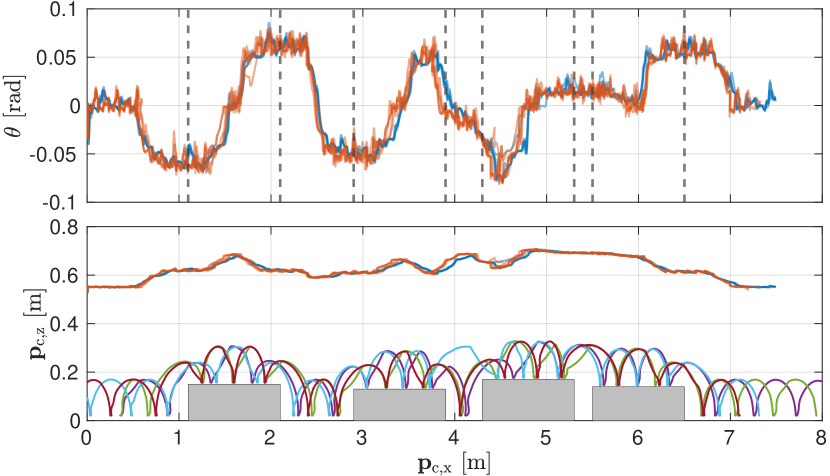
Figure 8: Simulation of pallet crossing scenario for five different trials commanding the robot to cross at 0.1 $\mathrm{m/s}$ (blue) and 0.05 $\mathrm{m/s}$ (red). The top graph shows the actual velocities (solid lines) and their respective references (dashed lines). The graph in the middle shows the pitch angle and the dashed vertical lines indicate the edges of the pallets for that specific location in the plot. The bottom graph shows the CoM $Z$ position for all the trials and the feet trajectories for one of the trials performed at 0.1 $\mathrm{m/s}$. The color of swings are related to the different legs.

VIII-B2 Walk into a V-shaped chimney

In this simulation we show HyQ walking at $0.03\,\mathrm{m/s}$ commanded velocity in the $X$ direction into a V-shaped chimney with friction coefficient $\mu=0.7$ and walls inclined at $35^{\circ}$ to the ground. This simulation exploits the cone constraints and force robustness cost defined inside the NMPC formulation that is vital for the success of this task. The robot receives online an update of the map of the environment through an on-board camera to get the information about the normals at the location of the contact. These normals are used to formulate the force robustness cost (2d) in the contact frame $\mathcal{K}$. With this cost, the NMPC provides optimal GRFs to stay close to the normals of the friction cones at the contacts.

As shown in the accompanying video, without the cone constraints the robot slips while climbing the chimney and ultimately falls. When the force robustness cost is enabled, the forces are regularized to stay in the middle of the cones, thanks to the robustness feature described in Section IV-C. In this case the robot walks successfully into the chimney. In Fig. 9, it can be seen that the longitudinal and lateral components of the GRF at the Left-Front (LF) foot stay within the bound $\mu f_{\mathrm{z}}$ (in red) imposed by the cone constraints. Moreover, Fig. 10 plots the normal versus the tangential force of the GRF together with the cone bound $\mu f_{\mathrm{z}}$ (red line). The picture shows that the GRF stays well within the bound without any violation. Therefore, including the force regularization term enables the NMPC to account for the estimation error in the orientation of contact normals and increase robustness to the external disturbances.

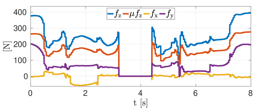
Figure 9: Walk into a V-shaped chimney simulation: GRFs of LF leg for a single gait cycle with cone constraints and regularization cost. Both the longitudinal $f_{\mathrm{x}}$ and lateral $f_{\mathrm{y}}$ lie conservatively within the bound $\mu f_{\mathrm{z}}$ imposed by cone constraints.

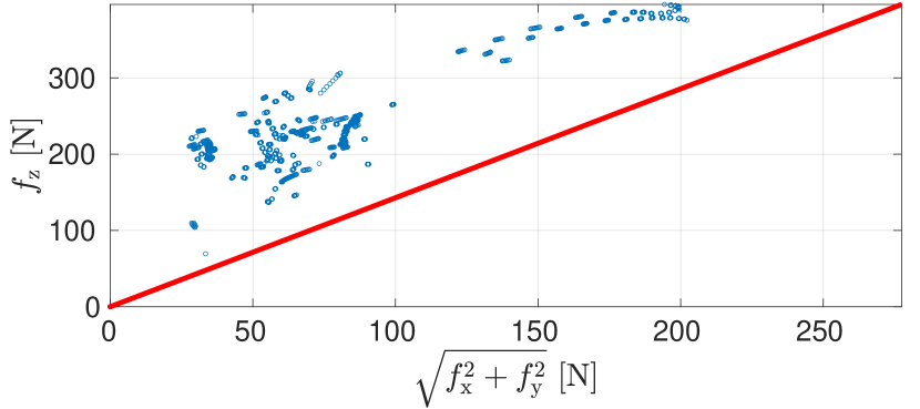
Figure 10: Walk into a V-shaped chimney simulation: Normal force $f_{z}$ versus tangential force $\sqrt{f_{\mathrm{x}}^{2}+f_{\mathrm{y}}^{2}}$ of the LF leg for a single gait cycle expressed in the contact frame. The red line is the cone bound $\mu f_{\mathrm{z}}$.

Apart from the simulation mentioned above, we also have added in the attached video, the simulations regarding the ZMP margin (see Section IV-B) and the importance of the re-planning at a higher rate. For the ZMP margin simulation, the robot is pushed with $200\,\mathrm{N}$ of lateral force for $1\,\mathrm{s}$ both in case of sufficient (higher weight on GRFs $Z$) and no (lower weight on GRFs $Z$) ZMP margin. The ZMP margin plots for this simulation can be seen in Fig. 11 where the ZMP margin is improved in case of the red line compared to the blue one because the GRFs $Z$ components are penalized relatively more ($100$ times) for the red line. Because of the improved margin the robot walks stably, whereas it falls while walking when there is no margin.

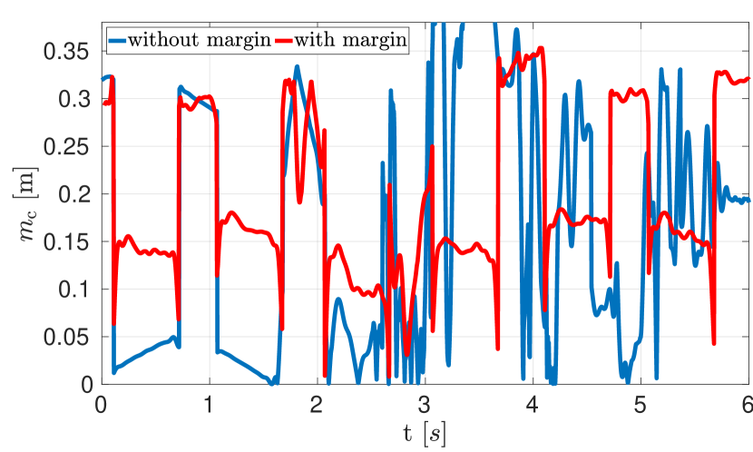
Figure 11: Plot of the ZMP margin $m_{\mathrm{c}}$ used to measure locomotion stability. The robot is pushed immediately after $2\,\mathrm{s}$ with lateral force of $200\,\mathrm{N}$ while walking on a flat terrain at $0.1\,\mathrm{m/s}$ CoM $X$ velocity. The discontinuities are due to the switching between 3/4 stance legs in a crawl gait.

In the second simulation, the robot is commanded with a constant CoM X velocity and heading velocity simultaneously. In case of re-planning at lower rate of $0.8\,\mathrm{Hz}$, the robot becomes unstable and falls due to increase in the model uncertainties and tracking errors. We would like to stress that when the re-planning is done at a lower frequency than $25\,\mathrm{Hz}$, the robot is in open-loop for the time interval between two consecutive re-planning instances, hence, it is no more NMPC but an online open-loop trajectory optimization. On the other hand, at a higher re-planning frequency of $25\,\mathrm{Hz}$ the robot walks successfully because the NMPC compensates for the model uncertainties and tracking errors.

VIII-C Experiments

We performed three different experiments to demonstrate the real-time implementation of our NMPC running on the on-board computer of the robot as follows.

VIII-C1 Omni-directional walk

With this experiment, we show the omni-directional walk performed by HyQ with the NMPC on a flat terrain. This experiment validates that the NMPC computes feasible trajectories after receiving different velocity commands from the user while walking. In this experiment, the robot was commanded with a longitudinal velocity ${}_{\mathcal{H}}\mathbf{v}_{\mathrm{c,x}}^{\mathrm{usr}}$ by the user to walk forward/backward and then a lateral velocity ${}_{\mathcal{H}}\mathbf{v}_{\mathrm{c,y}}^{\mathrm{usr}}$. Finally, a heading velocity $\omega^{\mathrm{usr}}_{\mathrm{z}}$ was commanded to turn in the left/right direction. Fig. 12 shows the CoM $X$-$Y$ position and yaw angle of the robot base and it can be noticed that the actual values track very closely the planned trajectories provided by the NMPC. Fig. 13 depicts the deviation of the actual velocities from the reference values while following the planned trajectories form NMPC. It can be seen in Fig. 14 that the GRFs generated by the WBC are compliant with the planned values $\mathbf{u}^{\mathrm{p}}$ and again the actual values of GRFs track closely the planned values. From these plots, it can be observed that the continuous re-planning with NMPC plays an important role to achieve good tracking of the planned trajectory.

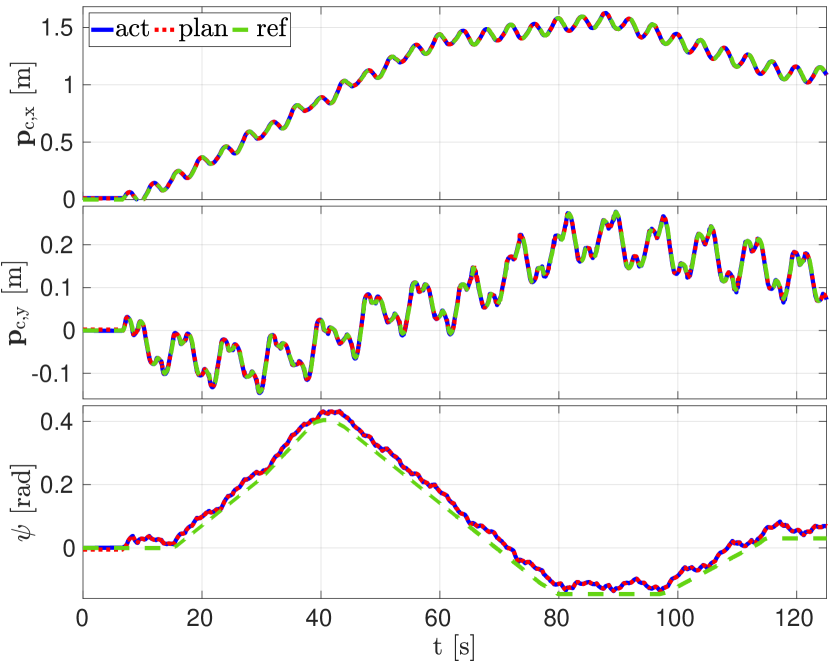
Figure 12: CoM X-Y position and yaw $\psi$ in omni-directional walk experiment. The blue, dotted red and dashed green line represent the actual, planned and reference values, respectively.

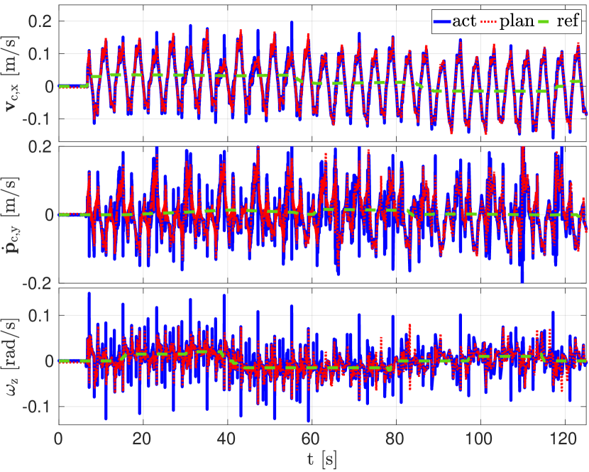
Figure 13: The longitudinal $\dot{\mathbf{p}}_{\mathrm{c,x}}$, lateral $\dot{\mathbf{p}}_{\mathrm{c,y}}$ and angular $\bm{\omega}_{\mathrm{z}}$ velocity of the robot in omni-directional walk experiment. The blue, dotted red and the green line represent the actual, planned and reference values, respectively.

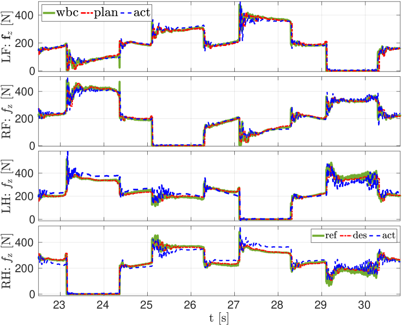
Figure 14: GRFs of one gait cycle in the omni-directional walk experiment (We show only one cycle for better visibility of the data). The green, dotted red and dashed blue line represent the output from WBC i.e., $f_{\mathrm{z},i}^{\mathrm{d}}$, planned and reference values, respectively.

VIII-C2 Traversing a static pallet

The purpose of this experiment was to demonstrate that the mobility cost (2c) incorporated in the NMPC formulation provides the necessary body pitch for the robot to traverse over a static pallet while maintaining good leg mobility. The pallet used in this experiment was $0.13\,\mathrm{m}$ in height and $0.8\,\mathrm{m}$ in length. Fig. 15 shows that the robot pitches up while climbing up the pallet and pitches down consequently while climbing down from the pallet. As shown in the attached video in simulation, when the mobility cost is deactivated, the NMPC maintains the horizontal base orientation. This causes a reduced hip-to-foot distance while stepping up/down on the pallet ultimately resulting in low leg mobility. When mobility cost is activated, it directs the NMPC solution to achieve the necessary pitch that allows to maintain the hip-to-foot distance at the reference value and hence the leg mobility is improved. Moreover, the VFA provides the corrected foot position (i.e., to avoid shin or feet collisions with the edges of the pallet) to the NMPC and this further enhances the overall locomotion.

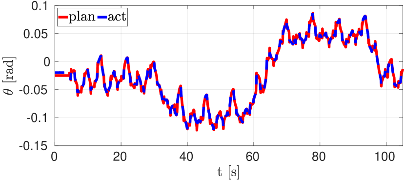
Figure 15: Planned (red) and Actual (dashed blue) pitch of the robot base while traversing a static pallet in the experiment at a commanded CoM $X$ velocity of $0.03\,\mathrm{m/s}$.

VIII-C3 Traversing a repositioned pallet

In this experiment we tested our NMPC to plan the robot motion in real-time by adapting the changes in the environment with the help of VFA. As it can be seen from the attached video, when the pallet ($0.13\,\mathrm{m}$ in height and $0.8\,\mathrm{m}$ in length) is pushed in front of HyQ while walking, the heightmap detects the pallet and the VFA provides updated foot locations to the NMPC. The NMPC after receiving these updated foot locations delivers a solution by pitching up the robot base in order to adapt to the change in the environment while maintaining the mobility. Even though the mobility cost is defined for the stance legs, it is interesting to notice that the NMPC decides to adjust the base pitch while swinging the RF leg onto the pallet (see Fig. 16) by forecasting the change in hip-to-foot distance at the touchdown. This experiment highlights the advantage of the predictive control over the traditional control apporaches for its ability to incorporate the knowledge of the future states. It also validates the effectiveness of our mobility cost in the NMPC coupled with the VFA to adapt to the changes in the locomotion environment.

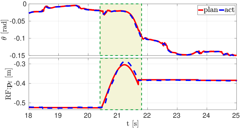
Figure 16: Robot base pitch achieved during the swing of RF leg while traversing a repositioned pallet in the experiment a commanded CoM $X$ velocity of $0.05\,\mathrm{m/s}$. The red and dashed blue line are planned and actual values.

IX Conclusion

In this work, we have demonstrated in experiments a real-time NMPC which leverages optimization of leg mobility to achieve terrain adaptation. The contact sequence parameters embedded inside the SRBD model allows us to encode the complementarity constraints directly, and without a need to enforce these constraints separately in the NMPC. We exploited the RTI scheme for our NMPC that enable us to close the loop at $25\,\mathrm{Hz}$ on the NMPC with a prediction horizon of $2\,\mathrm{s}$. Closing the loop on NMPC at $25\,\mathrm{Hz}$ allows us to compensate for the state drifts due to model uncertainties and tracking errors, and also adapt to the changes in the environment while following user velocity commands both in the simulations and experiments.

In our NMPC, the mobility cost penalizes the hip-to-foot distance from a reference value corresponding to a high mobility factor and hence it directs the NMPC to compute essential robot orientation to maintain a high mobility while respecting the kinematic limits. This is evident from the pallet experiments where we also included the VFA to correct undesired foot positions defined by the heuristics and avoid possible foot and shin collision. Accounting for the ZMP margin in our NMPC improved the locomotion stability of the robot in all of our experiments and simulation by keeping a sufficiently large ZMP margin from support polygon boundaries. Incorporating a force robustness term in the NMPC ensures that the GRFs stay close to the contact normals and hence, it enables the robot to cope with the estimation error of the orientation of the contact normals.

With our NMPC, we have performed successful dynamic locomotion in simulation as well as in the experiments on different rough terrains. In our future work we would like to extend our NMPC to optimize the step timing and foot locations. Additionally, the reference generator does not provide references by rejecting the external disturbances acting on the robot state, hence the robot complies transparently with these disturbances. Therefore, in the future we plan to empower the reference generator to reject disturbances to bring back the robot from a perturbed state to a state coherent with the user commands.

Appendix A Angular Velocity

We employ the $Z$-$Y$-$X$ convention [41] for the Euler angles sequence $\bm{\Phi}=(\phi,\,\theta,\,\psi)^{\top}$ to represent the orientation of the robot base where, $\phi$, $\theta$ and $\psi$ are the roll, pitch and yaw, respectively. The angular velocity in inertial and CoM frame is related to the Euler angle rates with the following relations:

$$\bm{\omega} =\mathbf{\bm{E}}(\bm{\Phi})\,\dot{\bm{\Phi}}$$ (22)

$${}_{\mathcal{C}}\bm{\omega} =\mathbf{\bm{E}}^{\prime}(\bm{\Phi})\,\dot{\bm{\Phi}}$$ (23)

$\mathbf{\bm{E}}(\bm{\Phi})$ and $\mathbf{\bm{E}}^{\prime}(\bm{\Phi})$ are the Euler angle rates matrix and conjugate Euler angle rates matrix respectively given by,

$$\mathbf{\bm{E}}(\bm{\Phi})=\begin{bmatrix}\cos(\theta)\cos(\psi)&-\sin(\psi)&0\\ \cos(\theta)\sin(\psi)&\cos(\psi)&0\\ -\sin(\theta)&0&1\end{bmatrix}$$ (24)

$$\mathbf{\bm{E}}^{\prime}(\bm{\Phi})=\begin{bmatrix}1&0&-\sin(\theta)\\ 0&\cos(\phi)&\cos(\theta)\sin(\phi)\\ 0&-\sin(\phi)&\cos(\theta)\cos(\phi)\end{bmatrix}$$ (25)

Remark: $\mathbf{\bm{E}}$ depends on pitch and yaw, whereas $\mathbf{\bm{E}}^{\prime}$ on roll and pitch. Thus, the Euler angle rates $\dot{\bm{\Phi}}$ is

$$\dot{\bm{\Phi}} =\mathbf{\bm{E}}^{-1}(\bm{\Phi})\,\bm{\omega}$$ (26)

$$\dot{\bm{\Phi}} =\mathbf{\bm{E}}^{\prime-1}(\bm{\Phi})\,{}_{\mathcal{C}}\bm{\omega}$$ (27)

Niraj Rathod received the Bachelor’s degree in Instrumentation and Control from College of Engineering Pune, India, in 2011. Immediately after bachelor’s he worked as a System Engineer in EEEC, Pune, India, until September 2014. Thereafter, he studied the Master’s in Automation and Control Engineering from Politecnico di Milano, Italy, and graduated in 2017. For his Master’s thesis he collaborated with RSE S.p.A., Milan, Italy. He is currently a PhD student at IMT School for Advanced Studies Lucca in Computer Science and System Engineering. During his PhD, he was an Affiliated Researcher at Dynamic Legged System (DLS), IIT, Genova, Italy. His research interests include MPC, Optimal Control, Control of Legged Robots and Hybrid Systems.

Angelo Bratta received his B.Sc. degree in control Engineering from the Politecnico di Bari, in 2017, and the M.Sc. degree in Mechatronics Engineering from the Politecnico di Torino, in 2019. In March 2019, he joined the Dynamic Legged Systems (DLS) lab at Istituto Italiano di Tecnologia (IIT) for his master thesis. Since November 2019 he is a Ph.D. student of the DLS. His research interests include robotics, controls, and online trajectory optimization.

Michele Focchi is currently a Researcher at the DLS team in IIT. He received both the Bsc. and the Msc. in Control System Engineering from Politecnico di Milano. After gaining some R&D experience in the industry, in 2009 he joined IIT where he developed a micro-turbine for which he obtained an international patent and a prize. In 2013, he got a PhD in robotics, getting involved in the Hydraulically Actuated Quadruped Robot (HyQ) project. He initially was developing torque controllers for locomotion purposes, subsequently he moved to higher level (whole-body) controllers and model identification. He was also investigating locomotion strategies that are robust to uncertainties and work reliably on the real platform. Currently his research interests are focused on pushing the performances of quadruped robots in traversing unstructured environments, by using optimization-based planning strategies to perform dynamic motion planning. He published more than 42 papers in international journals and conferences and supervised several master and PhD thesis.

Mario Zanon received the Master’s degree in Mechatronics from the University of Trento, and the Diplôme d’Ingénieur from the Ecole Centrale Paris, in 2010. After research stays at the KU Leuven, University of Bayreuth, Chalmers University, and the University of Freiburg he received the Ph.D. degree in Electrical Engineering from the KU Leuven in November 2015. He held a Post-Doc researcher position at Chalmers University until the end of 2017 and is now Assistant Professor at the IMT School for Advanced Studies Lucca. His research interests include numerical methods for optimization, economic MPC, optimal control and estimation of nonlinear dynamic systems, in particular for aerospace and automotive applications.

OCTAVIO VILLARREAL is currently a postdoctoral researcher at the Dynamic Legged System (DLS) lab of the Istituto Italiano di Tecnologia (IIT). He receive his MSc degree in Mechanical Engineering track Control Engineering from TUDelft in the Netherlands in 2016. He received his PhD from IIT and the University of Genoa on 2019 working at the DLS for his work on vision-based foothold adaptation and locomotion strategies for legged robots. His current research interests are related to control of legged robots, vision-based locomotion and foothold adaptation strategies, model predictive control for legged robots and trajectory optimization.

Claudio Semini (MSc 2005, PhD 2010) is the head of the Dynamic Legged Systems (DLS) lab at Istituto Italiano di Tecnologia (IIT) that developed a number of high-performance hydraulic robots, including HyQ, HyQ2Max, and HyQReal. He holds an MSc degree from ETH Zurich in electrical engineering and information technology. He spent 2 years in Tokyo for his research: MSc thesis at the Hirose Lab at Tokyo Tech and staff engineer at the Toshiba R&D center in Kawasaki working on mobile service robotics. During his PhD and subsequent PostDoc at IIT, he developed the quadruped robot HyQ and worked on its control. Since 2012 he leads the DLS lab. Claudio Semini is the author and co-author of more than 100 peer-reviewed publications in international journals and conferences and he received several awards for them. He is also a co-founder of the Technical Committee on Mechanisms and Design of the IEEE-RAS Society. He is/was the coordinator/partner of several EU-, National and Industrial projects (including HyQ-REAL, INAIL Teleop, Moog@IIT joint lab, ESA-ANT, etc). His research interests include the construction and control of highly dynamic and versatile legged robots for field application in real-world operations, locomotion, hydraulic drives, and others.

Alberto Bemporad received his Master’s degree in Electrical Engineering in 1993 and his Ph.D. in Control Engineering in 1997 from the University of Florence, Italy. In 1996/97 he was with the Center for Robotics and Automation, Department of Systems Science & Mathematics, Washington University, St. Louis. In 1997-1999 he held a postdoctoral position at the Automatic Control Laboratory, ETH Zurich, Switzerland, where he collaborated as a senior researcher until 2002. In 1999-2009 he was with the Department of Information Engineering of the University of Siena, Italy, becoming an Associate Professor in 2005. In 2010-2011 he was with the Department of Mechanical and Structural Engineering of the University of Trento, Italy. Since 2011 he is Full Professor at the IMT School for Advanced Studies Lucca, Italy, where he served as the Director of the institute in 2012-2015. He spent visiting periods at Stanford University, University of Michigan, and Zhejiang University. In 2011 he co-founded ODYS S.r.l., a company specialized in developing model predictive control systems for industrial production. He has published more than 400 papers in the areas of model predictive control, hybrid systems, optimization, automotive control, and is the co-inventor of 16 patents. He is author or coauthor of various software packages for model predictive control design and implementation, including the Model Predictive Control Toolbox (The Mathworks, Inc.) and the Hybrid Toolbox for MATLAB. He was an Associate Editor of the IEEE Transactions on Automatic Control during 2001-2004 and Chair of the Technical Committee on Hybrid Systems of the IEEE Control Systems Society in 2002-2010. He received the IFAC High-Impact Paper Award for the 2011-14 triennial and the IEEE CSS Transition to Practice Award in 2019. He is an IEEE Fellow since 2010.

References

- [1] M. H. Raibert, Legged robots that balance. MIT press, 1986.
- [2] J. Pratt, C.-M. Chew, A. Torres, P. Dilworth, and G. Pratt, “Virtual model control: An intuitive approach for bipedal locomotion,” The International Journal of Robotics Research, vol. 20, no. 2, pp. 129–143, 2001.
- [3] M. Focchi, R. Orsolino, M. Camurri, V. Barasuol, C. Mastalli, D. G. Caldwell, and C. Semini, Heuristic Planning for Rough Terrain Locomotion in Presence of External Disturbances and Variable Perception Quality. Springer International Publishing, 2020, pp. 165–209.
- [4] S. Fahmi, M. Focchi, A. Radulescu, G. Fink, V. Barasuol, and C. Semini, “STANCE: Locomotion adaptation over soft terrain,” IEEE Trans. Robot. (T-RO), vol. 36, no. 2, pp. 443–457, Apr. 2020.
- [5] C. D. Bellicoso, F. Jenelten, P. Fankhauser, C. Gehring, J. Hwangbo, and M. Hutter, “Dynamic locomotion and whole-body control for quadrupedal robots,” in 2017 IEEE/RSJ International Conference on Intelligent Robots and Systems (IROS), 2017, pp. 3359–3365.
- [6] S. Kuindersma, F. Permenter, and R. Tedrake, “An efficiently solvable quadratic program for stabilizing dynamic locomotion,” in 2014 IEEE International Conference on Robotics and Automation (ICRA), 2014, pp. 2589–2594.
- [7] M. Neunert, F. Farshidian, A. W. Winkler, and J. Buchli, “Trajectory Optimization Through Contacts and Automatic Gait Discovery for Quadrupeds,” IEEE Robot. Autom. Lett., vol. 2, no. 3, pp. 1502–1509, 2017.
- [8] M. Posa, S. Kuindersma, and R. Tedrake, “Optimization and stabilization of trajectories for constrained dynamical systems,” in 2016 IEEE International Conference on Robotics and Automation (ICRA), 2016, pp. 1366–1373.
- [9] B. Aceituno-Cabezas, C. Mastalli, D. Hongkai, M. Focchi, A. Radulescu, D. G. Caldwell, J. Cappelletto, J. C. Grieco, G. Fernando-Lopez, and C. Semini, “Simultaneous Contact, Gait and Motion Planning for Robust Multi-Legged Locomotion via Mixed-Integer Convex Optimization,” in IEEE Robot. Autom. Lett., 2018.
- [10] O. Melon, M. Geisert, D. Surovik, I. Havoutis, and M. Fallon, “Reliable trajectories for dynamic quadrupeds using analytical costs and learned initializations,” in 2020 IEEE International Conference on Robotics and Automation (ICRA), 2020, pp. 1410–1416.
- [11] M. Neunert, M. Stauble, M. Giftthaler, C. D. Bellicoso, J. Carius, C. Gehring, M. Hutter, and J. Buchli, “Whole-Body Nonlinear Model Predictive Control Through Contacts for Quadrupeds,” IEEE Robot. Autom. Lett., vol. 3, no. 3, pp. 1458–1465, 2018.
- [12] J. Koenemann, A. D. Prete, Y. Tassa, E. Todorov, O. Stasse, M. Bennewitz, and N. Mansard, “Whole-body model-predictive control applied to the HRP-2 humanoid,” in IEEE/RSJ Int. Conf. Intell. Robot. Syst., 2015, pp. 3346–3351.
- [13] H. Dai, A. Valenzuela, and R. Tedrake, “Whole-body Motion Planning with Simple Dynamics and Full Kinematics,” IEEE-RAS Int. Conf. Humanoid Robot., 2014.
- [14] D. E. Orin, A. Goswami, and S.-H. Lee, “Centroidal dynamics of a humanoid robot,” Auton. Robots, vol. 35, no. 2-3, pp. 161–176, jun 2013.
- [15] A. W. Winkler, C. D. Bellicoso, M. Hutter, and J. Buchli, “Gait and Trajectory Optimization for Legged Systems Through Phase-Based End-Effector Parameterization,” IEEE Robot. Autom. Lett., vol. 3, no. 3, pp. 1560–1567, 2018.
- [16] G. Bledt, P. M. Wensing, and S. Kim, “Policy-regularized model predictive control to stabilize diverse quadrupedal gaits for the mit cheetah,” in 2017 IEEE/RSJ International Conference on Intelligent Robots and Systems (IROS), 2017, pp. 4102–4109.
- [17] J. Di Carlo, P. M. Wensing, B. Katz, G. Bledt, and S. Kim, “Dynamic locomotion in the mit cheetah 3 through convex model-predictive control,” in 2018 IEEE/RSJ International Conference on Intelligent Robots and Systems (IROS), 2018, pp. 1–9.
- [18] T. Horvat, K. Melo, and A. J. Ijspeert, “Model predictive control based framework for com control of a quadruped robot,” in 2017 IEEE/RSJ International Conference on Intelligent Robots and Systems (IROS), 2017, pp. 3372–3378.
- [19] A. Herdt, H. Diedam, P. B. Wieber, D. Dimitrov, K. Mombaur, and M. Diehl, “Online walking motion generation with automatic footstep placement,” Advanced Robotics, vol. 24, no. 5-6, pp. 719–737, 2010.
- [20] R. Grandia, F. Farshidian, R. Ranftl, and M. Hutter, “Feedback mpc for torque-controlled legged robots,” in 2019 IEEE/RSJ International Conference on Intelligent Robots and Systems (IROS), 2019, pp. 4730–4737.
- [21] J. Hauser and A. Saccon, “A barrier function method for the optimization of trajectory functionals with constraints,” in Proceedings of the 45th IEEE Conference on Decision and Control, 2006, pp. 864–869.
- [22] G. Lantoine and R. P. Russell, “A hybrid differential dynamic programming algorithm for constrained optimal control problems. part 1: Theory,” Journal of Optimization Theory and Applications, vol. 154, no. 2, pp. 382–417, Aug 2012.
- [23] H. Li and P. M. Wensing, “Hybrid systems differential dynamic programming for whole-body motion planning of legged robots,” IEEE Robotics and Automation Letters, vol. 5, no. 4, pp. 5448–5455, 2020.
- [24] H. Bock and K. Plitt, “A multiple shooting algorithm for direct solution of optimal control problems*,” IFAC Proceedings Volumes, vol. 17, no. 2, pp. 1603–1608, 1984, 9th IFAC World Congress Budapest, Hungary, 2-6 July 1984.
- [25] M. Diehl, H. G. Bock, and J. P. Schlöder, “A real-time iteration scheme for nonlinear optimization in optimal feedback control,” SIAM J. Control Optim., vol. 43, no. 5, pp. 1714–1736, 2005.
- [26] R. Verschueren, G. Frison, D. Kouzoupis, N. van Duijkeren, A. Zanelli, B. Novoselnik, J. Frey, T. Albin, R. Quirynen, and M. Diehl, “Acados - A modular open-source framework for fast embedded optimal control,” arXiv, 2019.
- [27] F. Farshidian, E. Jelavic, A. Satapathy, M. Giftthaler, and J. Buchli, “Real-time motion planning of legged robots: A model predictive control approach,” in Humanoid Robot. (Humanoids), 2017 IEEE-RAS 17th Int. Conf. IEEE, 2017, pp. 577–584.
- [28] G. Bledt and S. Kim, “Implementing regularized predictive control for simultaneous real-time footstep and ground reaction force optimization,” in 2019 IEEE/RSJ International Conference on Intelligent Robots and Systems (IROS), 2019, pp. 6316–6323.
- [29] L. Sciavicco, B. Siciliano, and B. Sciavicco, Modelling and Control of Robot Manipulators, 2nd ed. Berlin, Heidelberg: Springer-Verlag, 2000.
- [30] P. Fankhauser, M. Bjelonic, C. Dario Bellicoso, T. Miki, and M. Hutter, “Robust rough-terrain locomotion with a quadrupedal robot,” in 2018 IEEE International Conference on Robotics and Automation (ICRA), 2018, pp. 5761–5768.
- [31] O. Cebe, C. Tiseo, G. Xin, H.-c. Lin, J. Smith, and M. Mistry, “Online Dynamic Trajectory Optimization and Control for a Quadruped Robot,” arXiv, 2020.
- [32] C. Semini, N. G. Tsagarakis, E. Guglielmino, M. Focchi, F. Cannella, and D. G. Caldwell, “Design of hyq - a hydraulically and electrically actuated quadruped robot,” IMechE Part I: Journal of Systems and Control Engineering, vol. 225, no. 6, pp. 831–849, 2011.
- [33] C. Mastalli, I. Havoutis, M. Focchi, D. G. Caldwell, and C. Semini, “Motion planning for quadrupedal locomotion: Coupled planning, terrain mapping and whole-body control,” IEEE Trans. Robot. (T-RO), pp. 1–14, 2020.
- [34] M. Diehl, H. G. Bock, H. Diedam, and P.-B. Wieber, “Fast Direct Multiple Shooting Algorithms for Optimal Robot Control,” in Fast Motions in Biomechanics and Robotics, Heidelberg, Germany, 2005.
- [35] S. Gros, M. Zanon, R. Quirynen, A. Bemporad, and M. Diehl, “From linear to nonlinear MPC: bridging the gap via the real-time iteration,” Int. J. Control, vol. 93, no. 1, pp. 62–80, 2020.
- [36] M. Focchi, A. del Prete, I. Havoutis, R. Featherstone, D. G. Caldwell, and C. Semini, “High-slope terrain locomotion for torque-controlled quadruped robots,” Auton. Robots, pp. 1–14, 2016.
- [37] T. Boaventura, J. Buchli, C. Semini, and D. Caldwell, “Model-based hydraulic impedance control for dynamic robots,” Robotics, IEEE Transactions on, vol. 31, no. 6, pp. 1324–1336, Dec 2015.
- [38] S. Nobili, M. Camurri, V. Barasuol, M. Focchi, D. G. Caldwell, C. Semini, and M. Fallon, “Heterogeneous sensor fusion for accurate state estimation of dynamic legged robots,” in Proceedings of Robotics: Science and Systems, Boston, USA, July 2017.
- [39] P. Fankhauser and M. Hutter, “A Universal Grid Map Library: Implementation and Use Case for Rough Terrain Navigation,” in Robot Operating System (ROS) – The Complete Reference (Volume 1), A. Koubaa, Ed. Springer, 2016, ch. 5.
- [40] A. B. Younes, J. D. Turner, D. Mortari, and J. L. Junkins, “A Survey of attitude error representations,” 2012.
- [41] J. Diebel, “Representing Attitude: Euler Angles, Unit Quaternions, and Rotation Vectors,” 2006.
- [42] R. Quirynen, “Numerical Simulation Methods for Embedded Optimization,” Thesis, no. January, p. 327, 2017.
- [43] J. C. Butcher, Numerical Methods for Ordinary Differential Equations. J. Wiley, 2003.
- [44] E. Hairer, S. Nørsett, and G. Wanner, Solving Ordinary Differential Equations I, 2nd ed., ser. Springer Series in Computational Mathematics. Berlin: Springer, 1993.
- [45] E. Hairer, S. Norsett, and G. Wanner, Solving Ordinary Differential Equations II – Stiff and Differential-Algebraic Problems, 2nd ed., ser. Springer Series in Computational Mathematics. Berlin: Springer, 1996.
- [46] O. Villarreal, V. Barasuol, P. M. Wensing, D. G. Caldwell, and C. Semini, “MPC-based controller with terrain insight for dynamic legged locomotion,” in 2020 IEEE International Conference on Robotics and Automation (ICRA), 2020, pp. 2436–2442.
- [47] M. Focchi, R. Featherstone, R. Orsolino, D. G. Caldwell, and C. Semini, “Viscosity-based height reflex for workspace augmentation for quadrupedal locomotion on rough terrain,” in 2017 IEEE/RSJ International Conference on Intelligent Robots and Systems (IROS), 2017, pp. 5353–5360.
- [48] T. Yoshikawa, “Analysis and Control of Robot Manipulators with Redundancy,” pp. 735–747, 1984.
- [49] C. Gehring, C. D. Bellicoso, S. Coros, M. Bloesch, P. Fankhauser, M. Hutter, and R. Siegwart, “Dynamic trotting on slopes for quadrupedal robots,” in 2015 IEEE/RSJ International Conference on Intelligent Robots and Systems (IROS), 2015, pp. 5129–5135.
- [50] G. Raiola, E. Mingo Hoffman, M. Focchi, N. Tsagarakis, and C. Semini, “A simple yet effective whole-body locomotion framework for quadruped robots,” Frontiers in Robotics and AI, vol. 7, p. 159, 2020.
- [51] P.-b. Wieber, “Trajectory free linear model predictive control for stable walking in the presence of strong perturbations,” in 2006 6th IEEE-RAS International Conference on Humanoid Robots, 2006, pp. 137–142.
- [52] T. Bretl and S. Lall, “Testing static equilibrium for legged robots,” IEEE Transactions on Robotics, vol. 24, no. 4, pp. 794–807, 2008.
- [53] O. Villarreal, V. Barasuol, M. Camurri, L. Franceschi, M. Focchi, M. Pontil, D. G. Caldwell, and C. Semini, “Fast and continuous foothold adaptation for dynamic locomotion through cnns,” IEEE Robotics and Automation Letters, vol. 4, no. 2, pp. 2140–2147, 2019.
- [54] R. Quirynen, M. Vukov, M. Zanon, and M. Diehl, “Autogenerating Microsecond Solvers for Nonlinear MPC: a Tutorial Using ACADO Integrators,” Optimal Control Applications and Methods, vol. 36, pp. 685–704, 2014.
- [55] G. Frison and M. Diehl, “HPIPM: a high-performance quadratic programming framework for model predictive control,” arXiv, 2020.
- [56] B. Abbyasov, R. Lavrenov, A. Zakiev, K. Yakovlev, M. Svinin, and E. Magid, “Automatic tool for gazebo world construction: from a grayscale image to a 3d solid model,” in 2020 IEEE International Conference on Robotics and Automation (ICRA), 2020, pp. 7226–7232.