Neural Trajectory Fields for Dynamic Novel View Synthesis

Abstract

Recent approaches to render photorealistic views from a limited set of photographs have pushed the boundaries of our interactions with pictures of static scenes. The ability to recreate moments, that is, time-varying sequences, is perhaps an even more interesting scenario, but it remains largely unsolved. We introduce DCT-NeRF, a coordinate-based neural representation for dynamic scenes. DCT-NeRF learns smooth and stable trajectories over the input sequence for each point in space. This allows us to enforce consistency between any two frames in the sequence, which results in high quality reconstruction, particularly in dynamic regions.

1 Introduction

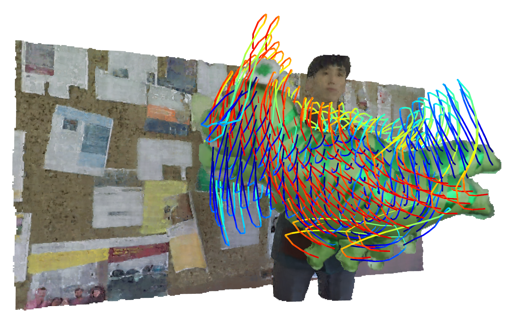
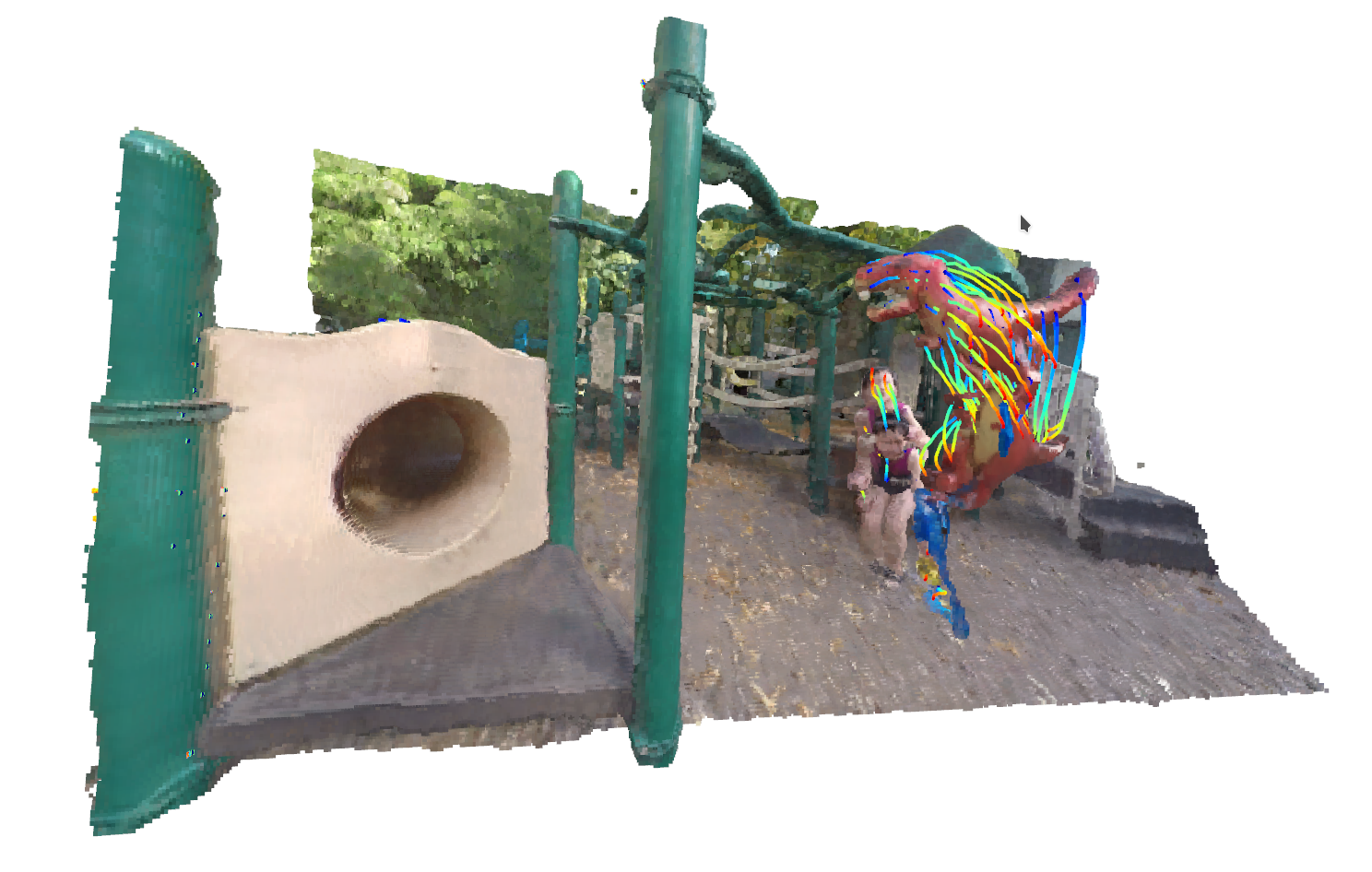
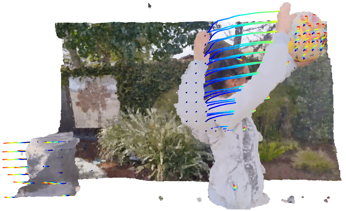
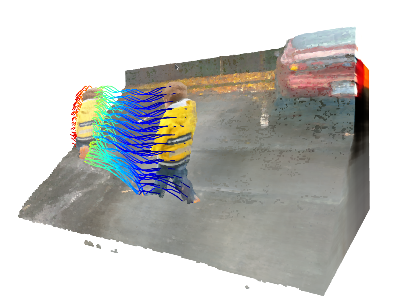
Figure 1: Our method predicts dense sequence-long trajectories for each point in the scene. Here we show examples of trajectories sampled at sparse locations. The 3D scenes are rendered by overlapping the radiance fields from two different frames of each sequence. The visualized 3D trajectories are directly estimated from the output of the first radiance field.

Novel view synthesis (NVS), the ability to create a photorealistic rendition of a scene from an unseen viewpoint, is a challenging, long-standing problem. After impressive early attempts [4, 17, 7], the computer vision and graphics communities made relatively slow progress towards a general and practical solution. That changed with the recent exploration of neural rendering [40], in particular the Neural Radiance Field (NeRF) [25], a coordinate-based neural representation for differentiable volumetric rendering which has since fueled a new wave of interest [20, 35, 41].

NeRF uses a multilayer perceptron (MLP), $\Psi$, to implicitly represent the geometry and radiance information of a static 3D scene. The color and transparency of a 3D point in space is estimated by querying the coordinates of the corresponding point and an associated viewing angle: $(\mathbf{c},\sigma)=\Psi(\mathbf{p},\mathbf{d})$. The network $\Psi$ is trained using a render-and-compare strategy, employing volumetric rendering from ray samples for view synthesis. NeRF makes an assumption common to most existing methods: the subject must be static so that the epipolar geometry constraints hold across views.

Generalizing NeRF for dynamic scenes captured from a single camera is challenging, as it requires disambiguating displacements due to parallax from those due to non-rigid motion. Recent pre-prints extend NeRF in one of two ways: they either parametrize time explicitly, i.e., $(\mathbf{c},\sigma)=\Psi(\mathbf{p},t,\mathbf{d})$ [18, 48], or they learn a warping field $\phi$ that maps the query coordinates at time $t$ to coordinates in a canonical frame, i.e., $(\mathbf{c},\sigma)=\Psi\left(\phi(\mathbf{p},t),\mathbf{d}\right)$ [43, 31]. When attempting to regularize the motion, these methods face a trade-off: broadly speaking, the more powerful the prior (e.g., the subject is a portrait [9]), the more stringent the assumptions on the scene content. On the other hand, more general priors (e.g., piece-wise linear motion [18]) tend to be weaker in enforcing consistency in dynamic regions.

This tension is not unique to NeRF, or even to NVS methods. A similar issue affects structure from motion (SfM) estimation. In that context, Akhter et al. argue that motion lives in space and time and can be tackled by using priors in either domain [1]. Motion, then, can be accounted for by using a combination of shape basis (space), which tend to be object-specific, or by using physical constraints on the trajectory (time), which are more object-agnostic [45, 53, 16]. Akhter et al. posit that using trajectories parameterized as a linear combination of sinusoidal bases (e.g., DCT transform) offers a good compromise between motion regularization and generality of the priors.

Inspired by this observation, we propose DCT-NeRF, a new spatiotemporal, coordinate-based neural scene representation. In addition to color and transparency, DCT-NeRF outputs continuous 3D trajectories across the whole input sequence: $(\mathcal{T},\mathbf{c},\sigma)=\Psi(\mathbf{p},t,\mathbf{d})$, where $\mathcal{T}$ is the discrete cosine transform trajectory of the point with spatiotemporal position $(\mathbf{p},t)$. As can be seen in Figure Neural Trajectory Fields for Dynamic Novel View Synthesis, this representation produces physically plausible motions that stay consistent across all frames, rather than simply predicting warping fields between neighboring frames. Moreover, in contrast to existing works, the trajectory field provides arbitrarily long spatiotemporal correspondence predictions that allow us to establish a principled regularization scheme.

Rendering views from significantly different times with our trajectory parametrization requires careful handling of two factors. First, we need to account for the potential change in reflectance of a point along its trajectory in both space and time. We do this by allowing the predicted color of a spacetime location to be a function of time. Second, we need to deal with regions that become occluded due to motion. Li et al. rely on a disocclusion mask learned for each pair of neighboring input images [18], but this approach does not scale when comparing any two frames in the sequence—the number of masks is combinatorial with respect to the sequence length. However, we note these problematic occlusion happen only when empty space at one time becomes occupied at another. This observation allows us to discard regions that may get occluded by dynamic objects simply by leveraging the transparency field $\sigma$, which our network already estimates for volumetric rendering.

Figure 1 shows examples of reconstructed radiance fields and trajectories. Note that the visualized trajectories are estimated by querying the network only at the time of the first frame, but capture the motion of objects over the entire sequence of frames. Our method produces high-quality renderings of dynamic scenes from novel viewpoints, both numerically and visually.

2 Related Work

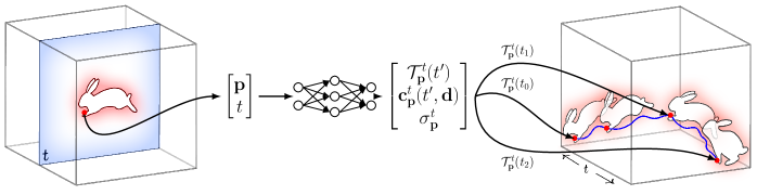
(a) Method Overview

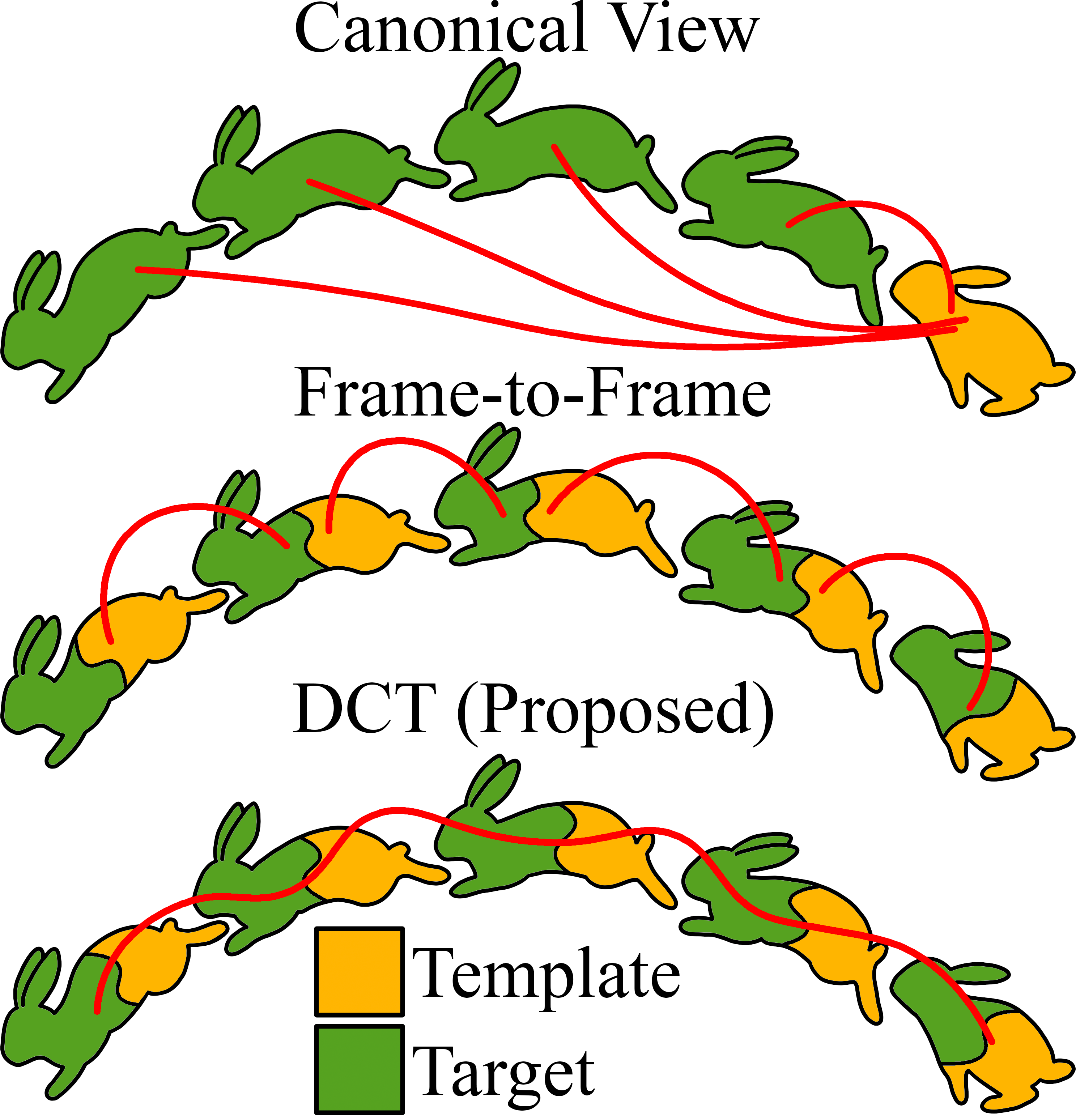
(b) Types of Warping

Figure 2: (a) We estimate the transparency $\sigma_{\mathbf{p}}^{t}$ and color $\mathbf{c}_{\mathbf{p}}^{t}$ for each spacetime location $(\mathbf{p},t)$ with viewing direction $\mathbf{d}$. $\mathbf{c}_{\mathbf{p}}^{t}$ is modeled as a temporal-view dependent function. To model the deformation of dynamic objects, we also predict the trajectory $\mathcal{T}_{\mathbf{p}}^{t}(\cdot)$ of any $(\mathbf{p},t)$, which allows us to follow the point as it moves through space and time. We parametrize $\mathcal{T}_{\mathbf{p}}^{t}$ as a DCT trajectory. (b) Existing approaches either define a canonical volume and warp all the frames to that one, or only warp neighboring frames. Thanks to our trajectories, our method can warp information from any frame to any frame.

Novel view synthesis. Early attempts at rendering a scene from an unseen view point date back several decades [10, 4, 17, 3, 7]. In part due to novel deep learning techniques, we have observed a proliferation of methods in just the last few years, which can be categorized based on the way they represent the scene.

A traditional approach is to estimate depth explicitly and use it to warp pixels, or learned features, from the input images to the novel view [14, 30, 6, 34]. Such scene representations offer flexibility, but inherit the shortcomings of depth-estimation algorithms, and require ways to explicitly deal with disocclusions at rendering time. Thanks to advances in single-image depth estimation, novel views can now even be generated from just a single image [47].

A second class of methods uses multiplane images (MPI) [52]. These algorithms learn a representation in which objects in the scene are associated to fronto-parallel layers. At inference time MPIs are warped and fused into a novel view. This approach implicitly regularizes depth and optimizes the layers to render the novel view. As a result, MPI-based methods produce impressive NVS results [52, 37, 8], even when using a single image as an input [44], or a single semantic map instead of an RGB image [11, 12].

The third and perhaps most promising strategy is to build an implicit neural representation of the scene [24, 5]. In their pioneering work, Mildenhall et al. propose to train a multilayer perceptron (MLP) that can predict color and transparency for each point in space given a viewing direction [25]. In just over a year since its publication, NeRF has inspired a number of follow-up works that tackle issues such as improved quality [50], performance [38, 19], or compositionality [33, 26].

Dynamic NVS. The problem of NVS is even more challenging for dynamic scenes because input views across time may capture differing scene geometry. A dynamic scene can be “frozen” into a static one by using synchronized cameras [54]. Single-image depth estimation also effectively allows one to freeze a scene. Luo et al. use it to compensate for small motion [21], while Yoon et al. use it to learn a full 4D representation of the scene, which they use to perform spatio-temporal image synthesis [49].

A number of pre-prints that augment NeRF for dynamic content have also recently appeared in parallel to our proposed research, which we report here for completeness. Many make simplifying assumptions, such as the availability of a depth estimate [48], or that dynamic objects are distractors to remove [23]. Other works target specific applications, such as self-portraits [29, 9]. Two closely related works are the works of Li et al., who use information from neighboring frames by learning a warping field [18], and Tretschk et al. who learn to warp input rays into a canonical volume [43].

The central idea for these methods, including ours, is that information must be warped between different time instants to combine information from multiple frames. Both Tretschk et al. [43] and Gao et al. [29] define a canonical space-time volume and warp the information from all the frames to this template, either by bending the light rays [43], or by applying a warping field to the values from the non-canonical frames [29]. Instead of defining a canonical volume, for each frame in the sequence Li et al. warp the information from the neighboring frames (i.e., $t\pm 1$, $t\pm 2$). In a way these are opposite extremes: the former two have a single “centralized” representation of the scene, where all the input frames are mapped to the same volume, and the latter can only gather and leverage local information. Our approach captures the advantages of both. Because we use trajectories, we can estimate dense correspondences and combine information from any two frames in the sequence (see Section 3.1.1). Figure 2(b) shows an illustration of the different strategies to combine dynamic information.

Non-rigid structure from motion. NRSfM concerns the problem of recovering deforming 3D shapes using 2D point correspondences from multiple images. Bregler et al. introduce this problem and propose the classical low-rank factorization approach[2]. Since then, two lines of work have emerged: shape-based and trajectory-based approaches. These two types of approaches are often complementary, and recent state-of-the-art employs both of them. Readers are referred to Jensen et al. [13] for a comprehensive evaluation of NRSfM methods. We focus our discussion on trajectory-based approaches for their relevance to our paper.

Torresani et al. utilize temporal information by imposing a linear motion model on top of a low-rank shape model, and show improvement on robustness against noise [42]. Since then, different trajectory priors have been explored. The seminal work of Akhteret et al. introduces a pure trajectory-based factorization method, which assumes that trajectories of different points in space can be represented as a linear combination of a small number of DCT trajectory bases [1]. Other methods have explored the convolutional structure of trajectories [53] as well as the assumption that different trajectories can be clustered into a small number of linear subspaces [16].

Taking inspiration from Akhteret et al., our approach represents continuous trajectories with DCT bases. A geometric analysis on how trajectories can be reconstructed using this representation is given by Park et al. [28]. One limitation to the low-rank approach of Akhteret et al. is that the number of DCT bases needs to be tuned per sequence. Valmadre et al. later argue that minimizing the response of high-pass filters (e.g., first- and second-difference filters) on trajectories eliminates the need to tune the number of bases, and also leads to more stable result for long sequences [45]. Following this insight, we minimize the difference between neighboring time steps on the trajectories without tuning the number of bases.

Occupancy flow. Niemeyer et al. propose a temporally and spatially continuous vector field to represent velocities [27]. To get the displacement of a point between different time steps, they need to integrate over the flow fields w.r.t. time, which leads to the number of queries of the network being proportional to time. In comparison, our trajectory field can output displacements between any time steps using only a single network query.

3 Method

We build on NeRF, an implicit neural representation that predicts the color $\mathbf{c}$ and the transparency $\sigma$ of any scene point, given a viewing direction [25]: $(\mathbf{c},\sigma)=\Psi(\mathbf{p},\mathbf{d})$. NeRF estimates the color of a pixel in the desired view via volumetric rendering along the corresponding ray. Given a number of posed views of a scene, NeRF can be trained by rendering pixels and comparing them with the corresponding ground-truth pixels. This training strategy, however, requires the scene to be static, as a dynamic point $\mathbf{p}$ maps to different pixels in the input views.

To account for the point’s motion, we propose to reconstruct its trajectory across the entire sequence. Inspired by classical works in the trajectory-based non-rigid structure from motion [1, 45], we parameterize the trajectory as a combination of sinusoidal bases, i.e., with a discrete cosine transform (DCT). A few observations are in order. First, a DCT trajectory is regular and smooth by construction, and has been shown to be a compact representation for the motion of deforming, dynamic objects [51, 22]. Second, all points in spacetime $(\mathbf{p},t)\in\mathbb{R}^{4}$ are associated with a DCT trajectory $\mathcal{T}_{\mathbf{p}}^{t}(\cdot)$, and trajectories associated with any two spacetime points, e.g., $(\mathbf{p}_{0},t_{0})$ and $(\mathbf{p}_{1},t_{1})$, are expected to be the same if they correspond to the same physical point, e.g., the tip of the bunny’s paw shown in Figure 2. This can be enforced by penalizing the difference between $\mathcal{T}_{\mathbf{p}_{0}}^{t_{0}}$ and the trajectory associated with $(\mathcal{T}_{\mathbf{p}_{0}}^{t_{0}}(t_{1}),t_{1})$ for any $\mathbf{p}_{0}$, $t_{0}$, and $t_{1}$. Finally, the ability to “move” the point in time following the trajectory allows us to compute the photometric error against the appropriate input pixels.

In the following we first formalize the description of our neural trajectory field, dubbed DCT-NeRF (see Section 3.1). We then show how the proposed representation is learned by enforcing photometric consistency through rendering with trajectories (see Section 3.2). The additional regularization terms we use are described in Section 3.3.

3.1 DCT-NeRF

Given a spacetime location $(\mathbf{p},t)$, our neural field outputs the DCT coefficients (or frequency values) $\boldsymbol{\varphi}$ for the trajectory, the embedding $\boldsymbol{\omega}$ for the temporal-view-dependent RGB color, and the transparency value $\sigma$:

$$(\boldsymbol{\varphi}_{\mathbf{p}}^{t},\boldsymbol{\omega}_{\mathbf{p}}^{t},\sigma_{\mathbf{p}}^{t})=\Psi(\mathbf{p},t),$$ (1)

where superscript $t$ and subscript $\mathbf{p}$ are added to each output to denote that they are associated to the spacetime location $(\mathbf{p},t)$. The outputs $\boldsymbol{\varphi}_{\mathbf{p}}^{t}$, $\boldsymbol{\omega}_{\mathbf{p}}^{t}$ are then used to condition the functional representation of the trajectory $\mathcal{T}_{\mathbf{p}}^{t}:\mathbb{R}\rightarrow\mathbb{R}^{3}$ and the color output $\mathbf{c}_{\mathbf{p}}^{t}:\mathbb{R}\times\mathbb{R}^{3}\rightarrow\mathbb{R}^{3}$, i.e.,

$$\mathcal{T}_{\mathbf{p}}^{t}(t^{\prime})=f_{\text{DCT}^{-1}}(t^{\prime},\boldsymbol{\varphi}_{\mathbf{p}}^{t}),~{}~{}~{}~{}~{}\mathbf{c}_{\mathbf{p}}^{t}(t^{\prime},\mathbf{d})=f_{\text{color}}(t^{\prime},\mathbf{d},\boldsymbol{\omega}_{\mathbf{p}}^{t}),$$ (2)

where $t^{\prime}$ is the time input to the functions, $f_{\text{DCT}^{-1}}$ is the inverse DCT transform of the DCT coefficients $\boldsymbol{\varphi}$ (details see Section 3.1.1), and $\mathbf{c}_{\mathbf{p}}^{t}$ is modeled as a neural network $f_{\text{color}}$. The details of the network architecture are given in Section 3.4. We note that, unlike the original NeRF, our color output for a spacetime location $(\mathbf{p},t)$ can vary over different time input $t^{\prime}$ to account for specularities or illumination changes, even with fixed $\mathbf{d}$. This is crucial when enforcing photometric consistency across large temporal distance in Section 3.2.2. In Figure 5, we show animations of images rendered by $\mathbf{c}_{\mathbf{p}}^{t}(t^{\prime},\mathbf{d})$ with varying time input $t^{\prime}$.

3.1.1 DCT Trajectory Representation

Given a sequence of $T$ frames, and the DCT coefficients $\boldsymbol{\varphi}\in\mathbb{R}^{3K}$ ($K<T$) associated with the trajectory $\mathcal{T}=[x(t),y(t),z(t)]$, we can compute the motion along the $x$ axis as:

$$x(t)=\sqrt{2/T}\sum_{k=1}^{K}\varphi_{x,k}\cos\left(\frac{\pi}{2T}(2t+1)k\right),$$ (3)

where $\varphi_{x,k}$ denotes the $k$-th coefficient for the $x$ axis. The $y$ and $z$ components of the trajectory have the same form. Equation 3 discards the $1^{\text{st}}$ component (i.e., $k=0$) of the inverse DCT transform. We choose this formulation to remove the global offset, since we only care about the relative displacement between points on the trajectory, i.e. $\Delta\mathbf{p}=\mathcal{T}(t_{1})-\mathcal{T}(t_{0})$. In our experiments we set $K=T-1$ for short sequences. For longer sequences, we use smaller $K$ for computational efficiency. Note that reducing the number of coefficients is a classical approach to enforce smoothness of the trajectory, but it requires knowing the complexity of the motion as a priori.

Training our network to directly predict the coefficients $\boldsymbol{\varphi}$ for each sampled spacetime location $(\mathbf{p},t)$ offers a convenient mechanism to enforce a single trajectory for each object point: the coefficients $\boldsymbol{\varphi}$ predicted for the same point at time $t_{0}$ and at time $t_{1}$ should be the same. Moreover, parameterizing a single trajectory for a point allows to predict the location of that point at any time $t$, whether that time instant was observed or not, see Figures Neural Trajectory Fields for Dynamic Novel View Synthesis and 1. This enables enforcing photometric consistency between any two frames, as discussed below.

3.2 Photometric Loss

3.2.1 Frame-wise photometric consistency ($\mathcal{L}^{\text{photo}}_{t_{0}}$)

Consider the color $\mathcal{C}^{t_{0}}$ of a pixel with ray direction $\mathbf{d}$ at time $t_{0}\in\{0,1,\cdots,T-1\}$. The contribution of a point along the ray $\mathbf{d}$ at position $\mathbf{p}$ to the color $\mathcal{C}^{t_{0}}$ on the camera plane is

$$\delta\mathcal{C}_{\mathbf{p}}^{t_{0}}=\sigma_{\mathbf{p}}^{t_{0}}\mathbf{c}_{\mathbf{p}}^{t_{0}}(t_{0},\mathbf{d}),$$ (4)

where we make the dependence on $\mathbf{p}$, the sampled time $t_{0}$, and $\mathbf{d}$ explicit. To render the corresponding pixel’s color, we swipe all the points along a ray, and perform volumetric rendering:

$$\mathcal{C}^{t_{0}}=\int_{\xi_{n}}^{\xi_{f}}A(\xi)\delta\mathcal{C}_{\mathbf{o}+\xi\mathbf{d}}^{t_{0}}d\xi,$$ (5)

where $A(\xi)=\exp\big{(}-\int_{\xi_{n}}^{\xi}\sigma_{\mathbf{o}+\nu\mathbf{d}}^{t_{0}}d\nu\big{)}$ accounts for the attenuation along the ray, and $\mathbf{o}$ denotes the origin of the ray.
Given the color $\mathcal{C}^{t_{0}}_{\text{GT}}$ of a pixel from the input image at time $t_{0}$, we use the rendered color from Equation 5 to compute the photometric loss:

$$\mathcal{L}^{\text{photo}}_{t_{0}}=\left\|\mathcal{C}^{t_{0}}-\mathcal{C}_{\text{GT}}^{t_{0}}\right\|_{2}^{2}.$$ (6)

3.2.2 Temporal photometric consistency ($\mathcal{L}^{\text{photo}}_{(t_{0};t_{1})}$)

Because we also estimate trajectories, we can integrate information from any other times, say time $t_{1}\in[0,T-1]$, in the same way that NeRF can compute the loss for any input frame despite the scene being dynamic. First, given a spacetime location $(\mathbf{p},t_{0})$, we compute its point correspondence at time $t_{1}$ as $\mathbf{p}^{\prime}=\mathbf{p}+\mathcal{T}_{\mathbf{p}}^{t_{0}}(t_{1})-\mathcal{T}_{\mathbf{p}}^{t_{0}}(t_{0})$. We can then follow Equation 4 and 5 to render pixels at time $t_{0}$ using the warped radiance field from time $t_{1}$:

$$\delta\mathcal{C}_{\mathbf{p}}^{(t_{0};t_{1})}=\sigma_{\mathbf{p}^{\prime}}^{t_{1}}\mathbf{c}_{\mathbf{p}^{\prime}}^{t_{1}}(t_{0},\mathbf{d}).$$ (7)

The final color $\mathcal{C}^{(t_{0};t_{1})}$ is computed with volumetric rendering by integrating $\delta\mathcal{C}_{\mathbf{p}}^{(t_{0};t_{1})}$ as in Equation 5. Temporal photometric consistency can then enforced by

$$\mathcal{L}^{\text{photo}}_{(t_{0};t_{1})}=\left\|\mathcal{C}^{(t_{0};t_{1})}-\mathcal{C}_{\text{GT}}^{t_{0}}\right\|_{2}^{2}.$$ (8)

(a)

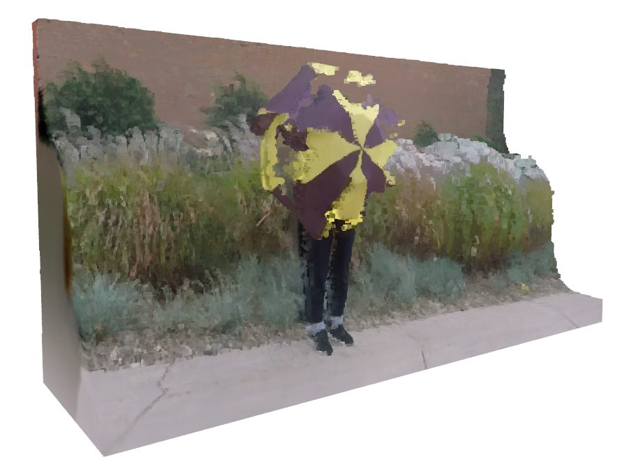
(b)

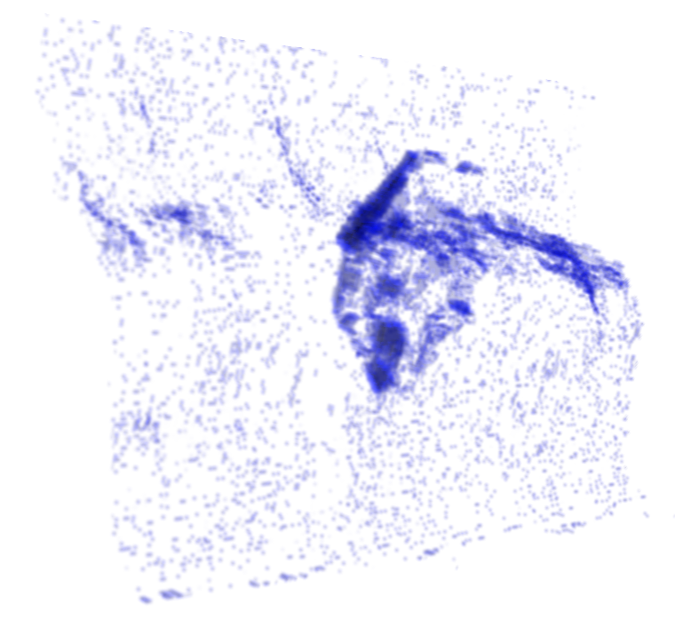
(c)

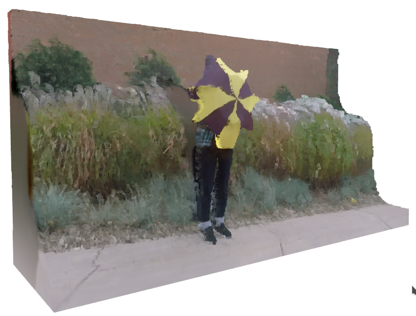
(d)

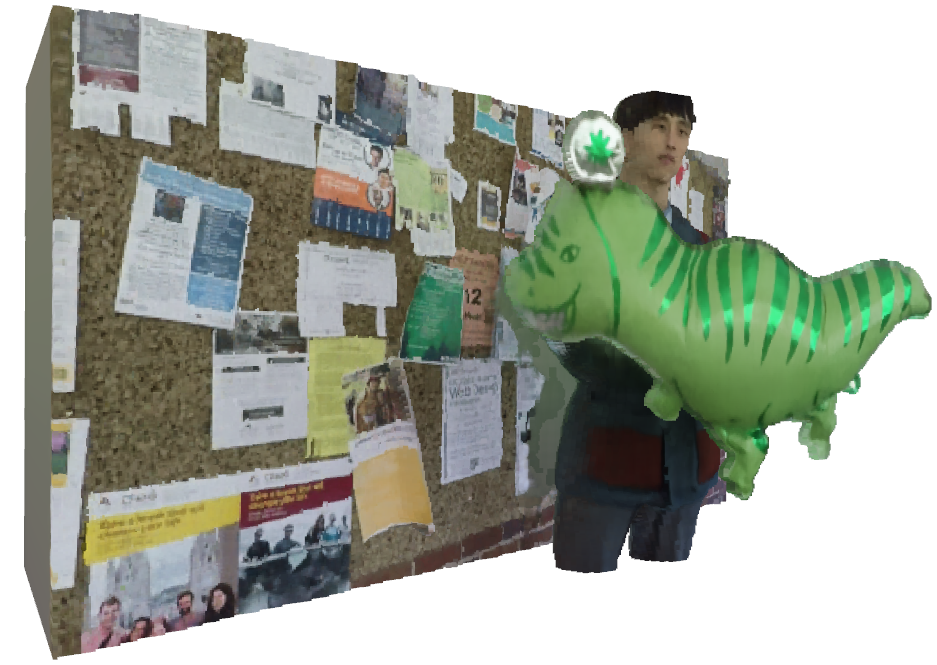
(e) Rend. at $t_{0}$

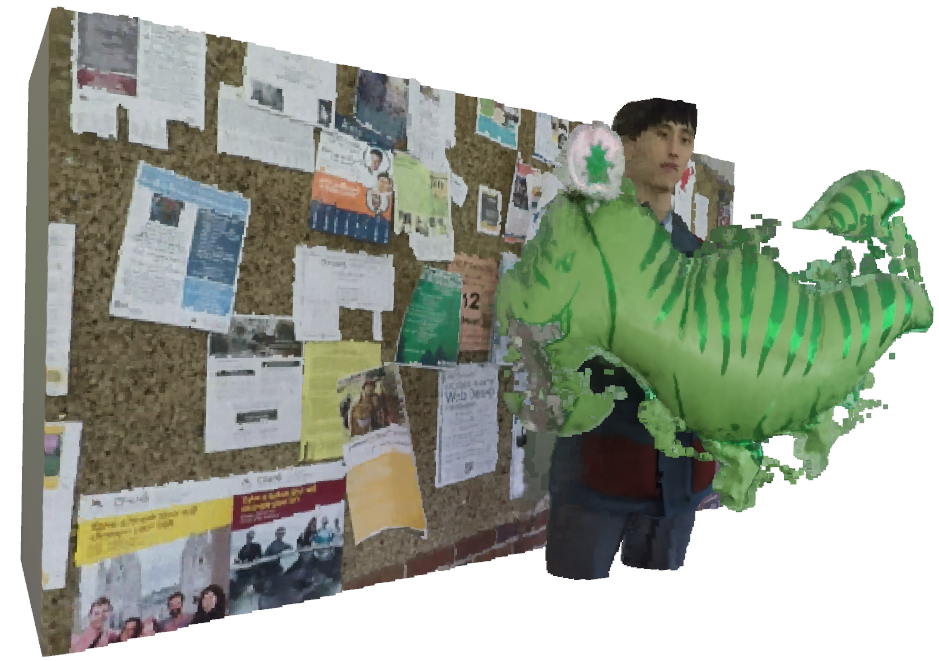
(f) Rend. w/o $p_{\text{occ}}$

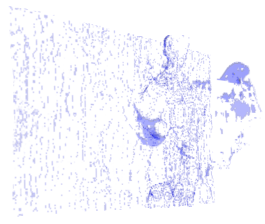
(g) $p_{\text{occ}}$

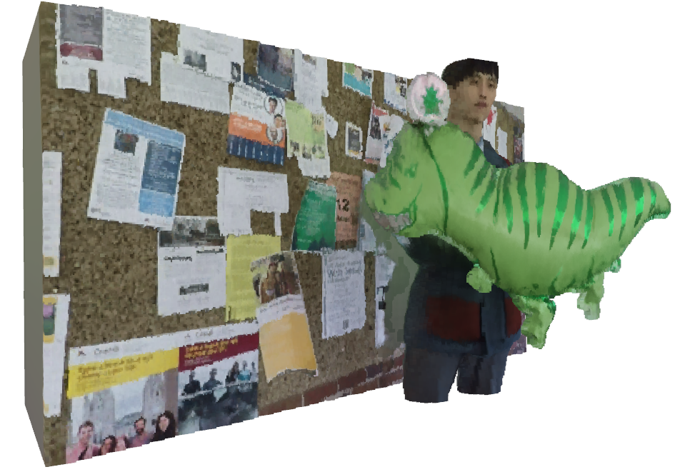
(h) Rend. w/ $p_{\text{occ}}$

Figure 3: Space that is empty at $t_{0}$ and becomes occupied at $t_{1}$ causes rendering issues (Rend. w/o $p_{\text{occ}}$). We predict the probability of a region to cause such issues ($p_{\text{occ}}$) and downweight their contribution to the rendering process accordingly (Rend. w/o $p_{\text{occ}}$).

Handling Temporal Occlusions.

Equation 7 does not account for temporal occlusions. Note that these regions are different from the typical spatial occlusions induced by the camera displacement. Consider a point $\mathbf{p}$ sampled in an empty area of the scene at time $t_{0}$, in other words $\sigma_{\mathbf{p}}^{t_{0}}=0$ and consequently $\delta\mathcal{C}^{t_{0}}_{\mathbf{p}}=0$. It is also expected that $\mathcal{T}_{\mathbf{p}}^{t_{0}}(t_{1})=0,\forall t_{1}$ since empty regions do not move, and thus $\mathbf{p}^{\prime}=\mathbf{p}$. Then suppose at some time $t_{1}$ an object moves and occupies position $\mathbf{p}$, which implies $\sigma_{\mathbf{p}^{\prime}}^{t_{1}}=\sigma_{\mathbf{p}}^{t_{1}}\neq 0$. Applying Equation 7 to this scenario yields

$$\delta\mathcal{C}^{(t_{0};t_{1})}_{\mathbf{p}}=\sigma_{\mathbf{p}}^{t_{1}}\mathbf{c}_{\mathbf{p}}^{t_{1}}(t_{0},\mathbf{d})\approx\delta\mathcal{C}_{\mathbf{p}}^{t_{1}}\ncong\delta\mathcal{C}_{\mathbf{p}}^{t_{0}}.$$ (9)

That is, even though $(\mathbf{p},t_{0})$’s trajectory is correctly estimated (zero motion), we use the wrong color when integrating Equation 5. One could identify and exclude these regions by learning a mask, as suggested by Li et al. [18]. However, comparing any two time stamps in the input sequence, as our method does, requires a combinatorial number of such maps. We observe that, barring interpenetration of objects, and neglecting objects that only appear in a subset of frames, this issue only manifests in space that is empty at $t_{0}$ and becomes occupied at another time $t_{1}$. Conveniently, our network predicts $\sigma$, which we use to estimate a probability of “empty-ness”:

$$p_{\text{e}}(\mathbf{p},t)=\text{sigmoid}(-k_{1}\sigma_{\mathbf{p}}^{t}+k_{2}),$$ (10)

where we empirically set $k_{1}=2$, and $k_{2}=3$. Treating $k_{1}$ and $k_{2}$ as learnable parameters results in equal or degraded quality. The probability that empty space at $(\mathbf{p},t_{0})$ becomes occluded at time $t_{1}$ can then be estimated as

$$p_{\text{occ}}(\mathbf{p},t_{0},t_{1})=p_{\text{e}}(\mathbf{p},t_{0})\big{(}1-p_{e}(\mathbf{p}^{\prime},t_{1})\big{)},$$ (11)

which we can use to modify Equation 7 to downweigh the contribution of occluded regions:

$$\delta\mathcal{C}^{(t_{0};t_{1})}_{\mathbf{p}}=p_{\text{occ}}(\mathbf{p},t_{0},t_{1})\cdot\delta\mathcal{C}^{t_{0}}_{\mathbf{p}}+\\ (1-p_{\text{occ}}(\mathbf{p},t_{0},t_{1}))\cdot\sigma_{\mathbf{p}^{\prime}}^{t_{1}}\mathbf{c}_{\mathbf{p}^{\prime}}^{t_{1}}(t_{0},\mathbf{d}).$$ (12)

Figure 3 shows a rendering of a frame using the warped radiance field from a different time, with and without $p_{\text{occ}}$ to handle occlusions. It also shows the probability $p_{\text{occ}}$ over the whole space.

3.3 Regularization

To encourage our system to converge to the correct solution, we follow the common practice of adding regularizers to our optimization.

Cycle consistency ($\mathcal{L}^{\text{cycle}}$). To enforce the network to make temporally consistent estimates, we add an $L_{1}$ loss on the difference of $(\mathcal{T},\mathbf{c},\sigma)$ for corresponding points, where $\mathcal{T}$ is represented by the DCT coefficients and the value of $\mathbf{c}$ is queried with the same $(\mathbf{d},t)$ input. To account for disocclusions, we weigh $\mathcal{L}^{\text{cycle}}$ by $1-p_{\text{occ}}$.

Single visible surface ($\mathcal{L}^{\text{SVS}}$). We want to encourage the source of radiance to be concentrated on a single surface area visible to the current view point. This means that most of the energy of the attenuation coefficient $A(\xi)$ in Equation 5 along the ray should be concentrated in a small window of size $r$:

$$\mathcal{L}^{\text{SVS}}=1-\max_{z_{0}}\int_{z=z_{0}}^{z=z_{0}+r}\tilde{A}(z)dz,$$ (13)

where $\tilde{A}$ denotes that $A$ is normalized to sum to one along the ray.

Trajectory regularizers ($\mathcal{L}^{\text{traj}}$). Our trajectory field is regularized by the combination of the following terms: (i) the spatial smoothness term, which calculates the $L_{1}$ norm of the spatial derivative of scene flow; (ii) an as-rigid-as-possible deformation loss [15], which is used to encourage the local deformation in occupied regions (measured by $p_{\text{e}}$) to be isometric; (iii) the temporal smoothness term which penalizes the $L_{1}$ norm of the scene flow.

Depth & flow. We use precomputed optical flow [39] to provide local supervision for the projection of $\mathcal{T}$ between neighboring frames. We also employ single-image depth estimation [32] to regularize $\sigma$ with a loss invariant to affine transformations [32, 46].

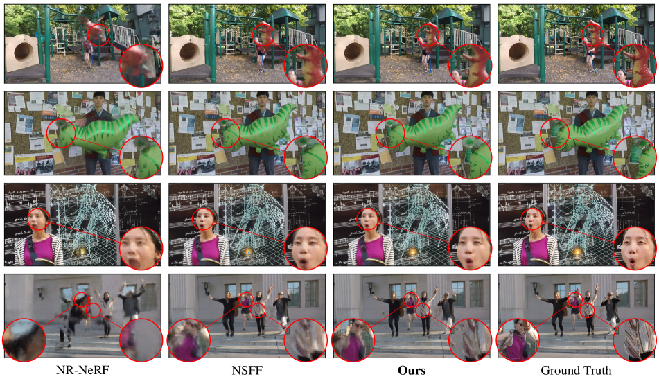
Figure 4: Comparisons. Our trajectory-based representation allows our method to perform well—particularly in dynamic regions.

3.4 Implementation

Optimization objective. Given a pixel sampled at time $t_{0}$, we compute the loss as a combination of photometric losses and regularization terms. The photometric loss is evaluated as the sum of $\mathcal{L}^{\text{photo}}_{t_{0}}+\mathcal{L}^{\text{photo}}_{(t_{0};t_{0}\pm 1)}+\mathcal{L}^{\text{photo}}_{(t_{0};t_{1})}$, which enforces the rendering consistency between neighboring time steps, as well as a randomly sampled time step $t_{1}$. We employ a local-to-global strategy to sample $t_{1}$. That is, during the initial optimization iterations, $t_{1}$ is limited to $[t_{0}-2,t_{0}+2]$. We then exponentially increase the temporal radius during optimization, until the sample range of $t_{1}$ covers the whole sequence.

We find that adjusting the weights for certain regularization terms during the different stages of the optimization is critical for their success. First, when the weights for the depth and optical flow loss are not linearly decreased, as proposed by Li $\emph{et al}.\hbox{}$ [18], the network may be forced to overfit to the noise in the pre-computed depth and optical flow maps. Second, gradually increasing the weight of $\mathcal{L}^{\text{svs}}$ from a small value, e.g., $1e-5$, helps to prevent getting stuck in poor local minima in the early stage of training. We use the same hyperparameters for all our experiments, and the details are included in the supplementary.

Static background. The consistency of the background across time is crucial for the viewing experience of dynamic NVS. Martin-Brualla et al. show success in learning a rigid NeRF for static background from images with dynamic objects [23]. Their approach is to modify the rigid NeRF model to output an additional 3D blending field so as to exclude interference from the dynamic regions of input images. Similarly, Li et al. [18] also include a rigid NeRF and blend the rigid and dynamic radiance fields to render an additional image when evaluating the photometric loss. We follow the approach of Li et al. and observe an improvement in the stability of the background.

Network architecture. We adapt the architecture from the original NeRF [25] implementation, with the following changes: (i) we concatenate an additional positional encoding of time to the input; (ii) parallel to the linear layers that predict $\sigma$, we add another linear layer to output the DCT coefficients; (iii) we concatenate the directional inputs with the positional encoding of time when calculating the color.

4 Evaluation and Results

[trim=0 0 0 0,width=autoplay,loop]10figures/spacetime_radiance_anim/0000000023

Figure 5: For photometric consistency across time in the presence of dynamic specularities and shadows, our approach allows the predicted radiance to be rendered with respect to any other reference time across the sequence. Given the leftmost column’s time in the sequence as a reference, the rightmost two columns show two different points in spacetime but rendered using the predicted radiance values of the reference time. To view this animation, please open this document in a media-enabled PDF viewer, such as Adobe Reader.

Datasets. We use eight diverse scenes from the NVIDIA Dynamic Scene Dataset [49] to validate our method with both numerical and visual comparisons. For each scene, the dataset provides 12 sequences captured by synchronized cameras at fixed positions. Then camera motion is synthesized by choosing frames from different cameras at each time step. We extract 24 frames per scene as input sequences for training, and report results on the held-out 11 images for each frame.

Trajectories. Figure Neural Trajectory Fields for Dynamic Novel View Synthesis shows the trajectory estimated at the time of the first frame traced out over the whole duration of the sequence. Notice that our trajectories are stable and smooth across the entire sequences, even when the motion changes direction, as is the case of the scene on the right. The trajectories can be sampled as densely or as sparsely as needed. Figure 1 shows trajectories for the same sequences of Figure Neural Trajectory Fields for Dynamic Novel View Synthesis and two more overlaid to a 3D visualization of the radiance field computed by our method.

Dynamic specularities and shadows. Because we allow the color $\mathbf{c}$ to vary with time, we can render one frame with the radiance of another. Figure 5 shows an example of this (please view the animation in a media-enabled reader). In this experiment, we apply the radiance of a reference frame (the leftmost in the figure) to two different target frames, animated over the entire sequence. Notice how the dynamically changing specularities and shadows correctly correspond to the reference image. This is possible because our method correctly estimates both radiance and trajectories over time.

Ablation study. We analyze the impact of the regularization terms we describe in Section 3.3 on the overall quality of the results. We use our model trained without the static background loss as a baseline. Table 1 shows the numerical results when using only the neighboring frames for $\mathcal{L}^{\text{photo}}$ (“local only”), removing the occlusion weights ($p_{\text{occ}}$), and removing other regularization terms one at a time. Through our numerical analysis, as well as a thorough visual inspection of the results, we observe that these terms are statistically beneficial. Removing any of them from our formulation introduces some artifacts in some of the results. However, they are not central to our results. We refer the reader to the supplementary material for visual examples.

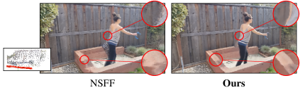
Figure 6: Comparison with Li et al. [18] on a challenging NVS case where we render the view on one end of the trajectory using the camera on the opposite end. The cameras are shown in the inset. Our method produces fewer artifacts in particular in the temporal occlusion regions.

Comparisons. The two most closely related methods are the method by Li et al. [18] and that of Tretschk et al. [43]. Both of these methods are pre-prints and we compare against them to offer context to the reader.

Table 1 shows a numerical comparison against these two methods, and two more [36, 21] whose numbers were reported by Li et al. [18]. The numbers show that we perform significantly better than the first three methods in the table. We perform roughly on par with Li et al., with their method performing slightly better overall, and ours performing slightly better on the dynamic regions. This is consistent with the fact that our main contribution is a global representation of the motion of the dynamic regions of the scene. We offer a per-sequence breakdown of the comparison with the two most closely related methods in Table 2.

Figure 4 shows visual comparisons with Li et al. and Tretschk et al. Note how our method produces sharper results in many of the dynamic regions. We also show a comparison with the method by Li et al. on two additional sequences in Figure 6. These are two challenging cases in which the rendered view is at the location of the camera at one end of the capture sequence, but the values are from the time of the camera at the opposite end of the sequence. Thanks to the fact that we model long-term trajectories, we can better reconstruct the scene.

Another approach for NVS of dynamic scenes is the method by Yoon et al. [49]. Note that their method requires a mask for the dynamic regions to be given. As their code is not publicly available we compare against their work by selecting a few frames from their own videos and synthesize a reasonably close view in space and time with our method. Their results are overall sharper, which is consistent with the general observation that NeRF-based methods can be a bit blurrier. However, several artifacts can be seen in their results around depth discontinuity regions.

Limitations. Dynamic NVS from single camera is a very challenging task, and the quality of our result is sensitive to the context and motion of the input scene. Figure 8 shows two typical failure cases for our method. Our method may confuse specularity as dynamic motion and have trouble to track very thin objects with fast motion. Our method also shares the same limitations as other NeRF-based approaches: it requires long training per scene ($\approx$12hrs on 2 RTX2080 GPUs for a short sequence with 24 frames) and has a limited ability to recover high frequency dynamic details. As with others, we are also susceptible to degenerate cases of camera / object motion.

Some of the images we use in the paper are courtesy of Li et al. [18] and the Nvidia Dynamic Scene Dataset [49].

Method	Full scene		Dynamic parts only
	SSIM ($\uparrow$)	LPIPS ($\downarrow$)	SSIM ($\uparrow$)	LPIPS ($\downarrow$)
3D Photo [36]	0.614	0.215	0.486	0.217
Luo et al. [21]	0.746	0.141	0.530	0.207
NR-Nerf [43]	0.526	0.307	0.40	0.400
NSFF [18]	0.928	0.045	0.758	0.097
Ours w/o static	0.885	0.077	0.701	0.092
- local only	0.878	0.087	0.689	0.103
- w/o $p_{\text{occ}}$	0.889	0.078	0.707	0.097
- w/o $\mathcal{L}^{\text{cycle}}$	0.881	0.082	0.718	0.103
- w/o $\mathcal{L}^{\text{svs}}$	0.885	0.082	0.711	0.096
- w/o $\mathcal{L}^{\text{traj}}$	0.879	0.085	0.701	0.101
- w/o $\mathcal{L}^{\text{depth}}$	0.892	0.081	0.697	0.108
Ours (w static)	0.915	0.049	0.704	0.089

Table 1: Numerical results and ablation study for our method. We perform better than existing methods and on par with the concurrent method by Li et al. [18].

Sequence	NR-NeRF [43]	NSFF [18]	Ours
	full / dyn.	full / dyn.	full / dyn.
Balloon1	0.278 /0.398	0.062/0.175	0.051/ 0.146
Balloon2	0.301 /0.395	0.030/0.065	0.054/ 0.074
DynamicFace	0.164 /0.175	0.025/0.034	0.021/ 0.022
Jumping	0.415 /0.518	0.046/0.111	0.056/ 0.116
Playground	0.363 /0.467	0.066/0.124	0.055/ 0.092
Skating	0.349 /0.575	0.017/0.061	0.036/ 0.088
Truck	0.268 /0.346	0.026/0.052	0.025/ 0.036
Umbrella	0.315 /0.322	0.089/0.157	0.091/ 0.134

Table 2: Breakdown of LPIPS metric per scene from the Nvidia Dynamic Scene Dataset.

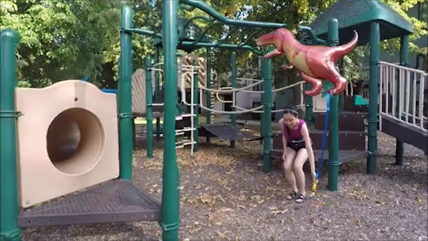
(a)

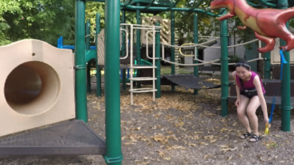
(b)

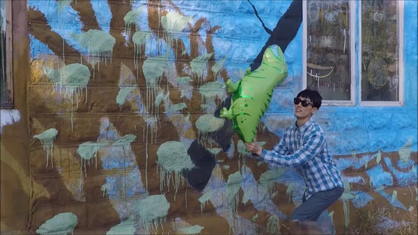
(c)

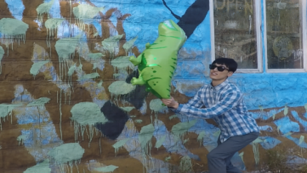
(d)

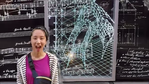
(e) Yoon et al. [49]

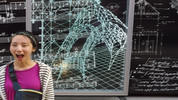
(f) Ours

Figure 7: The code from Yoon et al. is not available. We estimate the location and time of a frame from their results and synthesize it with our method. Note the artifacts at disocclusion regions, e.g., the front-most green pole in the top row, or the right side of the woman in the bottom.

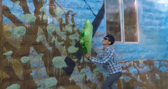
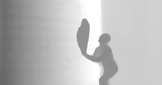
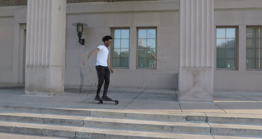
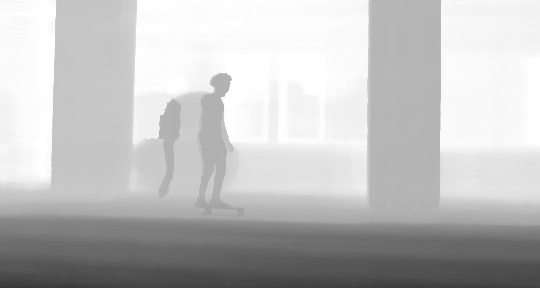
Figure 8: Failure cases for our method. Top: confuse background as moving region. Bottom: artifacts due to fast motion.

5 Conclusions

We present DCT-NeRF, a new coordinate-based neural representation that can render photorealistic novel views of dynamic scenes. Our core contribution is the design of a dense trajectory field representation that captures the motion of dynamic parts of the scene over the entire input sequence. Using a parametrization based on the discrete cosine transform (DCT), our trajectories are continuous and stable across the entire sequence. Further, we show how one can perform photometrically consistent sampling across arbitrary points in time by combining these parametric trajectory estimates with disocclusion prediction, and we use this technique to leverage information from any input image for any output image, ultimately producing compelling renditions of dynamic scenes.

Appendix A Implementation details

We use 10 frequencies for the spatial-temporal positional encoding, and use 4 frequencies for the directional and temporal input to the color output layer. Both the radiance field and the DCT trajectories are defined in normalized device coordinates (NDC). We linearly sample 128 depth values along the rays when performing volumetric rendering. Due to the intense computational cost of the current method, we do not perform additional depth sampling and train an extra “fine” network as done by Mildenhall et al. [25].

A.1 Regularization details

$\mathcal{L}^{\text{cycle}}$ details. Given a point $\mathbf{p}_{t_{0}}$ at time $t_{0}$, by query the DCT trajectory $\mathcal{T}_{\mathbf{p}_{t_{0}}}^{t_{0}}$ outputted by $\Psi(\mathbf{p}_{t_{0}},t_{0})$, we get its correspondences at time $t_{1}$, i.e. $\mathbf{p}_{t_{1}}=\mathcal{T}_{\mathbf{p}_{t_{0}}}^{t_{0}}(t_{1})$. Denote the occupancy, color and DCT coefficients associated to the points $\mathbf{p}_{t_{i}}$ as $(\sigma_{t_{i}},\mathbf{c}_{t_{i}},\boldsymbol{\varphi}_{t_{i}})$, and with particular note that $\mathbf{c}_{t_{0}}=\mathbf{c}[\mathbf{p}_{t_{0}},t_{0}](t_{0})$ and $\mathbf{c}_{t_{1}}=\mathbf{c}[\mathbf{p}_{t_{1}},t_{1}](t_{0})$, the cycle consistency loss is evaluated as:

$$\mathcal{L}^{\text{cycle}}=(1-p_{\text{occ}})(\|\boldsymbol{\varphi}_{t_{0}}-\boldsymbol{\varphi}_{t_{1}}\|_{1}+0.1\|\sigma_{t_{0}}-\sigma_{t_{1}}\|_{1}\\ +0.1\|\mathbf{c}_{t_{0}}-\mathbf{c}_{t_{1}}\|_{1}),$$ (14)

where $p_{\text{occ}}$ is the probability of $\mathbf{p}_{t_{0}}$ being disoccluded by $\mathbf{p}_{t_{1}}$ as an empty region.

$\mathcal{L}^{\text{traj}}$ details. Given neighboring points $\mathbf{p}_{t_{0}}$ and $\mathbf{p}_{t_{0}}^{\prime}$ (converted from NDC to Euclidean coordinates) along a ray at time $t_{0}$, the trajectory regularization loss is evaluated as:

$$\mathcal{L}^{\text{traj}} =\underbrace{\|(\mathbf{p}_{t_{0}}-\mathbf{p}_{t_{0}\pm 1})-(\mathbf{p}_{t_{0}}^{\prime}-\mathbf{p}_{t_{0}\pm 1}^{\prime})\|_{1}}_{\text{spatial smoothness of scene flow.}}$$ (15)

$$+\underbrace{(1-p_{\text{e}})(\|(\mathbf{p}_{t_{0}}-\mathbf{p}_{t_{0}})^{\prime}-(\mathbf{p}_{t_{1}}-\mathbf{p}_{t_{1}}^{\prime})\|_{1})}_{\text{as-rigid-as-possible.}}$$

$$+\underbrace{\|(\mathbf{p}_{t_{0}}-\mathbf{p}_{t_{0}\pm 1})-(\mathbf{p}_{t_{0}}^{\prime}-\mathbf{p}_{t_{0}\pm 1}^{\prime})\|_{1}}_{\text{temporal smoothness of trajectory / small scene flow.}}.$$

Hyperparameters. The full regularization loss is linearly combined as:

$$\mathcal{L}^{\text{cycle}}+0.1\mathcal{L}^{\text{traj}}+w_{\text{SVS}}\mathcal{L}^{\text{SVS}}+w_{\text{depth}}\mathcal{L}^{\text{depth}}+w_{\text{flow}}\mathcal{L}^{\text{flow}},$$ (16)

where the initial $w_{\text{depth}}$ and $w_{\text{flow}}$ are set as 0.04 and 0.02, and then decreased by a factor of 0.1 every 7 epochs. $w_{\text{SVS}}$ is increased by a factor of 10 every 7 epochs from the initial value of $1e-5$, until it reaches $1e-2$.

A.2 Optimization details

We use Adam optimizer with default parameters, and set the learning rate as $5e-4$ for the first 70 epochs, then decrease the learning rate by 0.1 for the next 10 epochs for fine-tuning. For the temporal local-to-global procedure, we increase the temporal radius by 2 times every 10 epochs.
We use a batch size of $1024+512$ during training, with the first 1024 pixels uniformly sampled from training images, while the last 512 pixels are sampled uniformly only from the regions marked by a motion segmentation method. Sampling extra pixels from moving regions is also done by Li et al. [18], and we note that this is helpful to speed up convergence for small non-rigid regions, but not crucial to the end result of our method.

Appendix B Visual comparison for the ablation study

The visual comparison of different versions of the method for the ablation study is provided in Figure 9.

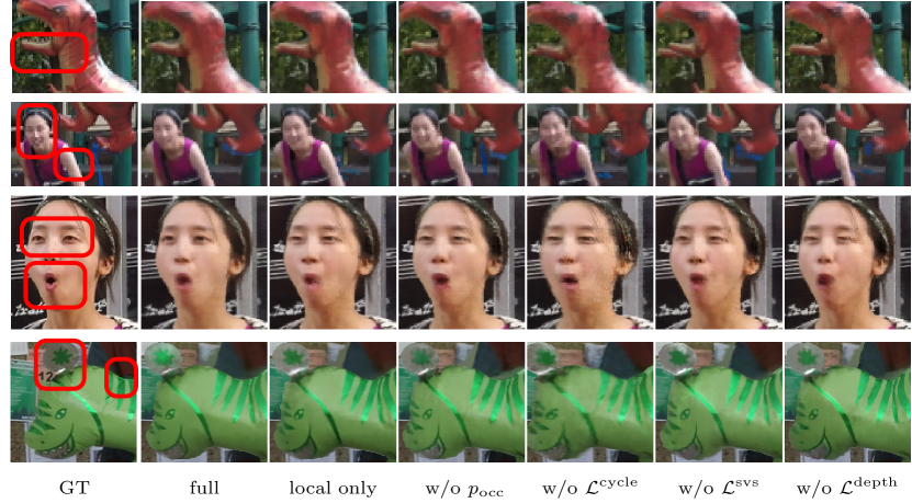
Figure 9: Visual comparison for ablation studies. The regions which show major difference between different versions of the method are marked with red rectangles.

References

- [1] Ijaz Akhter, Yaser Sheikh, Sohaib Khan, and Takeo Kanade. Trajectory space: A dual representation for nonrigid structure from motion. IEEE Transactions on Pattern Analysis and Machine Intelligence (TPAMI), 2010.
- [2] Christoph Bregler, Aaron Hertzmann, and Henning Biermann. Recovering non-rigid 3d shape from image streams. In IEEE Conference on Computer Vision and Pattern Recognition (CVPR), 2000.
- [3] Chris Buehler, Michael Bosse, Leonard McMillan, Steven Gortler, and Michael Cohen. Unstructured lumigraph rendering. In ACM Transactions on Graphics (SIGGRAPH), 2001.
- [4] Shenchang Eric Chen and Lance Williams. View interpolation for image synthesis. In ACM Transactions on Graphics (SIGGRAPH), 1993.
- [5] Zhiqin Chen and Hao Zhang. Learning implicit fields for generative shape modeling. In IEEE Conference on Computer Vision and Pattern Recognition (CVPR), 2019.
- [6] Inchang Choi, Orazio Gallo, Alejandro Troccoli, Min H Kim, and Jan Kautz. Extreme view synthesis. In IEEE International Conference on Computer Vision (ICCV), 2019.
- [7] Paul E Debevec, Camillo J Taylor, and Jitendra Malik. Modeling and rendering architecture from photographs: A hybrid geometry-and image-based approach. In ACM Transactions on Graphics (SIGGRAPH), 1996.
- [8] John Flynn, Michael Broxton, Paul Debevec, Matthew DuVall, Graham Fyffe, Ryan Overbeck, Noah Snavely, and Richard Tucker. DeepView: View synthesis with learned gradient descent. In IEEE Conference on Computer Vision and Pattern Recognition (CVPR), 2019.
- [9] Chen Gao, Yichang Shih, Wei-Sheng Lai, Chia-Kai Liang, and Jia-Bin Huang. Portrait neural radiance fields from a single image. arXiv preprint arXiv:2012.05903, 2020.
- [10] Ned Greene. Environment mapping and other applications of world projections. In IEEE Computer Graphics and Applications (CGA), 1986.
- [11] Tewodros Habtegebrial, Varun Jampani, Orazio Gallo, and Didier Stricker. Generative view synthesis: From single-view semantics to novel-view images. Advances in Neural Information Processing Systems (NeurIPS), 2020.
- [12] Hsin-Ping Huang, Hung-Yu Tseng, Hsin-Ying Lee, and Jia-Bin Huang. Semantic view synthesis. In European Conference on Computer Vision (ECCV), 2020.
- [13] Sebastian Hoppe Nesgaard Jensen, Mads Emil Brix Doest, Henrik Aanæs, and Alessio Del Bue. A benchmark and evaluation of non-rigid structure from motion. International Journal of Computer Vision (IJCV), 2021.
- [14] Nima Khademi Kalantari, Ting-Chun Wang, and Ravi Ramamoorthi. Learning-based view synthesis for light field cameras. In ACM Transactions on Graphics (SIGGRAPH), 2016.
- [15] Suryansh Kumar, Yuchao Dai, and Hongdong Li. Monocular dense 3D reconstruction of a complex dynamic scene from two perspective frames. In IEEE International Conference on Computer Vision (ICCV), 2017.
- [16] Suryansh Kumar, Yuchao Dai, and Hongdong Li. Spatio-temporal union of subspaces for multi-body non-rigid structure-from-motion. 2017.
- [17] Marc Levoy and Pat Hanrahan. Light field rendering. In ACM Transactions on Graphics (SIGGRAPH), 1996.
- [18] Zhengqi Li, Simon Niklaus, Noah Snavely, and Oliver Wang. Neural scene flow fields for space-time view synthesis of dynamic scenes. arXiv preprint arXiv:2011.13084, 2020.
- [19] David B Lindell, Julien NP Martel, and Gordon Wetzstein. AutoInt: Automatic integration for fast neural volume rendering. arXiv preprint arXiv:2012.01714, 2020.
- [20] Lingjie Liu, Jiatao Gu, Kyaw Zaw Lin, Tat-Seng Chua, and Christian Theobalt. Neural sparse voxel fields. In Advances in Neural Information Processing Systems (NeurIPS), 2020.
- [21] Xuan Luo, Jia-Bin Huang, Richard Szeliski, Kevin Matzen, and Johannes Kopf. Consistent video depth estimation. ACM Transactions on Graphics, 2020.
- [22] Wei Mao, Miaomiao Liu, Mathieu Salzmann, and Hongdong Li. Learning trajectory dependencies for human motion prediction. 2019.
- [23] Ricardo Martin-Brualla, Noha Radwan, Mehdi SM Sajjadi, Jonathan T Barron, Alexey Dosovitskiy, and Daniel Duckworth. NeRF in the wild: Neural radiance fields for unconstrained photo collections. 2020.
- [24] Lars Mescheder, Michael Oechsle, Michael Niemeyer, Sebastian Nowozin, and Andreas Geiger. Occupancy networks: Learning reconstruction in function space. In IEEE Conference on Computer Vision and Pattern Recognition (CVPR), 2019.
- [25] Ben Mildenhall, Pratul P. Srinivasan, Matthew Tancik, Jonathan T. Barron, Ravi Ramamoorthi, and Ren Ng. NeRF: Representing scenes as neural radiance fields for view synthesis. In European Conference on Computer Vision (ECCV), 2020.
- [26] Michael Niemeyer and Andreas Geiger. GIRAFFE: Representing scenes as compositional generative neural feature fields. arXiv preprint arXiv:2011.12100, 2020.
- [27] Michael Niemeyer, Lars Mescheder, Michael Oechsle, and Andreas Geiger. Occupancy flow: 4d reconstruction by learning particle dynamics. In IEEE Conference on Computer Vision and Pattern Recognition (CVPR), 2019.
- [28] Hyun Soo Park, Takaaki Shiratori, Iain Matthews, and Yaser Sheikh. 3d reconstruction of a moving point from a series of 2d projections. In European Conference on Computer Vision (ECCV), 2010.
- [29] Keunhong Park, Utkarsh Sinha, Jonathan T. Barron, Sofien Bouaziz, Dan B Goldman, Steven M. Seitz, and Ricardo Martin-Brualla. Deformable neural radiance fields. arXiv preprint arXiv:2011.12948, 2020.
- [30] Eric Penner and Li Zhang. Soft 3D reconstruction for view synthesis. In ACM Transactions on Graphics (SIGGRAPH), 2017.
- [31] Albert Pumarola, Enric Corona, Gerard Pons-Moll, and Francesc Moreno-Noguer. D-NeRF: Neural radiance fields for dynamic scenes. arXiv preprint arXiv:2011.13961, 2020.
- [32] René Ranftl, Katrin Lasinger, David Hafner, Konrad Schindler, and Vladlen Koltun. Towards robust monocular depth estimation: Mixing datasets for zero-shot cross-dataset transfer. IEEE Transactions on Pattern Analysis and Machine Intelligence (TPAMI), 2020.
- [33] Daniel Rebain, Wei Jiang, Soroosh Yazdani, Ke Li, Kwang Moo Yi, and Andrea Tagliasacchi. DeRF: Decomposed radiance fields. arXiv preprint arXiv:2011.12490, 2020.
- [34] Gernot Riegler and Vladlen Koltun. Stable view synthesis. arXiv preprint arXiv:2011.07233, 2020.
- [35] Katja Schwarz, Yiyi Liao, Michael Niemeyer, and Andreas Geiger. GRAF: Generative radiance fields for 3D-aware image synthesis. In Advances in Neural Information Processing Systems (NeurIPS), 2020.
- [36] Meng-Li Shih, Shih-Yang Su, Johannes Kopf, and Jia-Bin Huang. 3D photography using context-aware layered depth inpainting. In IEEE Conference on Computer Vision and Pattern Recognition (CVPR), 2020.
- [37] Pratul P Srinivasan, Richard Tucker, Jonathan T Barron, Ravi Ramamoorthi, Ren Ng, and Noah Snavely. Pushing the boundaries of view extrapolation with multiplane images. In IEEE Conference on Computer Vision and Pattern Recognition (CVPR), 2019.
- [38] Matthew Tancik, Ben Mildenhall, Terrance Wang, Divi Schmidt, Pratul P Srinivasan, Jonathan T Barron, and Ren Ng. Learned initializations for optimizing coordinate-based neural representations. arXiv preprint arXiv:2012.02189, 2020.
- [39] Zachary Teed and Jia Deng. RAFT: Recurrent all-pairs field transforms for optical flow. In European Conference on Computer Vision (ECCV), 2020.
- [40] Ayush Tewari, Ohad Fried, Justus Thies, Vincent Sitzmann, Stephen Lombardi, Kalyan Sunkavalli, Ricardo Martin-Brualla, Tomas Simon, Jason Saragih, Matthias Nießner, et al. State of the art on neural rendering. In Computer Graphics Forum, 2020.
- [41] A. Tewari, O. Fried, J. Thies, V. Sitzmann, S. Lombardi, K. Sunkavalli, R. Martin-Brualla, T. Simon, J. Saragih, M. Nießner, R. Pandey, S. Fanello, G. Wetzstein, J.-Y. Zhu, C. Theobalt, M. Agrawala, E. Shechtman, D. B Goldman, and M. Zollhöfer. State of the Art on Neural Rendering. 2020.
- [42] Lorenzo Torresani, Aaron Hertzmann, and Chris Bregler. Nonrigid structure-from-motion: Estimating shape and motion with hierarchical priors. IEEE Transactions on Pattern Analysis and Machine Intelligence (TPAMI), 2008.
- [43] Edgar Tretschk, Ayush Tewari, Vladislav Golyanik, Michael Zollhöfer, Christoph Lassner, and Christian Theobalt. Non-rigid neural radiance fields: Reconstruction and novel view synthesis of a deforming scene from monocular video. arXiv preprint arXiv:2012.12247, 2020.
- [44] Richard Tucker and Noah Snavely. Single-view view synthesis with multiplane images. In IEEE Conference on Computer Vision and Pattern Recognition (CVPR), 2020.
- [45] Jack Valmadre and Simon Lucey. General trajectory prior for non-rigid reconstruction. In IEEE Conference on Computer Vision and Pattern Recognition (CVPR), 2012.
- [46] Chaoyang Wang, Simon Lucey, Federico Perazzi, and Oliver Wang. Web stereo video supervision for depth prediction from dynamic scenes. In International Conference on 3D Vision (3DV), 2019.
- [47] Olivia Wiles, Georgia Gkioxari, Richard Szeliski, and Justin Johnson. SynSin: End-to-end view synthesis from a single image. In IEEE Conference on Computer Vision and Pattern Recognition (CVPR), 2020.
- [48] Wenqi Xian, Jia-Bin Huang, Johannes Kopf, and Changil Kim. Space-time neural irradiance fields for free-viewpoint video. arXiv preprint arXiv:2011.12950, 2020.
- [49] Jae Shin Yoon, Kihwan Kim, Orazio Gallo, Hyun Soo Park, and Jan Kautz. Novel view synthesis of dynamic scenes with globally coherent depths from a monocular camera. In IEEE Conference on Computer Vision and Pattern Recognition (CVPR), 2020.
- [50] Kai Zhang, Gernot Riegler, Noah Snavely, and Vladlen Koltun. NeRF++: Analyzing and improving neural radiance fields. arXiv preprint arXiv:2010.07492, 2020.
- [51] Yan Zhang, Michael J Black, and Siyu Tang. We are more than our joints: Predicting how 3D bodies move. arXiv preprint arXiv:2012.00619, 2020.
- [52] Tinghui Zhou, Richard Tucker, John Flynn, Graham Fyffe, and Noah Snavely. Stereo Magnification: Learning view synthesis using multiplane images. In ACM Transactions on Graphics (SIGGRAPH), 2018.
- [53] Yingying Zhu and Simon Lucey. Convolutional sparse coding for trajectory reconstruction. IEEE Transactions on Pattern Analysis and Machine Intelligence (TPAMI), 2013.
- [54] C. Lawrence Zitnick, Sing Bing Kang, Matthew Uyttendaele, Simon A. J. Winder, and Richard Szeliski. High-quality video view interpolation using a layered representation. In ACM Transactions on Graphics (SIGGRAPH), 2004.