SPUX Framework: a Scalable Package for Bayesian Uncertainty Quantification and Propagation

Abstract

We present SPUX - a modular framework for Bayesian inference enabling uncertainty quantification and propagation in linear and nonlinear, deterministic and stochastic models, and supporting Bayesian model selection. SPUX can be coupled to any serial or parallel application written in any programming language, (e.g. including Python, R, Julia, C/C++, Fortran, Java, or a binary executable), scales effortlessly from serial runs on a personal computer to parallel high performance computing clusters, and aims to provide a platform particularly suited to support and foster reproducibility in computational science. We illustrate SPUX capabilities for a simple yet representative random walk model, describe how to couple different types of user applications, and showcase several readily available examples from environmental sciences. In addition to available state-of-the-art numerical inference algorithms including EMCEE, PMCMC (PF) and SABC, the open source nature of the SPUX framework and the explicit description of the hierarchical parallel SPUX executors should also greatly simplify the implementation and usage of other inference and optimization techniques.

1 Introduction

For centuries, human intuition and curiosity toward natural phenomena have been the main driving forces behind the discovery of the fundamental laws of physics, and behind the formulations of mathematical models capable of describing past and forecasting future behavior of various complex systems. In evironmental sciences, in particular, there are strong justifications, and thus a strong trend, for using stochastic models, such as stochastic differential equations (SDEs) and individual based models (IBMs), to simulate the dynamical systems of interest. Indeed, these models are especially useful when intrinsic uncertainties are present as in, for instance, the modeling of inter-connected systems such as climate, weather, ocean and lake dynamics, subsurface ground water flows, hydrological catchments, urban floods, and ecological communities, to name a few.

In recent years, as reviewed in [GDB⁺19], two additional important influencing factors have arisen and have become available to scientists: considerable computational power and a massive increase in data availability. The steady increase in computational power has allowed models to reduce their level of approximation to reality by increasing complexity and/or by achieving faster convergence towards the exact solution. Concurrently, the recent technological advances in sensing and imaging have initiated the so-called era of big data, allowing one to complement mechanistic modeling based on first principles (e.g. conservation laws) and human ingenuity with observational data [KBBP16].

However, the opportunity to use high performance computing (HPC) infrastructures to enable an efficient coupling of complex models and/or of large data-sets, is posing significant challenges to the so-called scientific programming and computing practices. Indeed, nowadays users are often required to run their forward simulations on HPC clusters, while developers need to be able to exploit different types of parallelism to ensure the feasibility of model calibration and uncertainty propagation. It is also worth noting, that while for some complex models already a single forward simulation can be computationally expensive, the statistical inference methodologies for assimilating datasets can be extremely demanding already for models of intermediate complexity.

By building on these necessities, the focus of our contribution is on describing a new software framework, called SPUX, which stands for "Scalable Package for Uncertainty Quantification in X", that aims to abstract and simplify the access to modern computing infrastructure for reproducible uncertainty quantification and propagation. The remainder of this section is dedicated to exposing basic information about Bayesian inference, which is at the core of SPUX (a more detailed exposure is provided in section 2), and to briefly reviewing similar existing computational suites.

To advance the scientific understanding of complex systems, statistical inference techniques such as Bayesian inference [GCS⁺14] can be used for probabilistic quantification (i.e. including uncertainties) of model parameters and (past, present and future) model states, and for comparing several available models using Bayesian model selection. Bayesian inference conditions the prior distributions of model parameters and (stochastic model) states (which probabilistically describe any prior information regarding model parameter and output values) on the data to get the corresponding posterior distributions. For instance, it can be based on the so-called likelihood function for a given model, which formulates the model as a probability distribution of observations for given model parameter values (to which model’s inputs and outputs are associated), and on the prior distribution of model parameter values. Posterior probability distribution of model parameters can then be inferred from combining such prior knowledge about the model and its parameters with the likelihood function (see Bayes theorem and section 2 for more details).

Historically, the successful application of Bayesian inference for stochastic generative models with realistic datasets has been hindered by the lack of efficient sampling techniques for posterior model trajectories and for the computationally expensive evaluation of the likelihood (as a high-dimensional integration). The development of methodologies to address such challenges has been an active research topic in recent years. Relevant methods include Particle Filter (PF) estimation (with optional trajectory "smoothing" techniques [DJ09]) coupled with Markov Chain Monte Carlo (MCMC) sampling - also known as Particle Markov Chain Monte Carlo (PMCMC) [ADH10], Gibbs sampling - including Conditional Ornstein-Uhlenbeck Sampling (COUS) [RM09], the Approximate Bayesian Computation (ABC) methodologies such as Simulated Annealing ABC (SABC) [AKS15], Hamiltonian Monte Carlo [AUS16], and stochastic variational (Bayesian) inference (SVI) methods [HBWP13].

In recent years, the number of computational inference frameworks implementing the above-mentioned methodologies to study not only deterministic but also stochastic models has been growing considerably. An attempt to provide a thorough review of those suites would certainly fall short, unless carried out as a dedicated review, and is therefore beyond the scope of this contribution. Instead, we briefly mention the existing approaches that we are aware of to provide a context and to highlight their specificities, referring the reader to the individual articles. In particular, the first table overviews UQ suites targeted at "static" stochastic models, where uncertainty is specified by means of hierarchical Bayesian networks, or incorporated into boundary (and initial) conditions or forcing terms:

Name	Language	Type	Type	Methodologies	Reference
BUGS	R/SAS	partial	specialized	Gibbs sampler	[LSTB09]
JAGS	Python/R	partial	specialized	Gibbs sampler	[Plu04]
MUQ	C++	partial	framework	optimization and UQ	[PCDM14]
Pest	proprietary	partial	program	optimization and UQ	[DMRT14]
STAN	Python	partial	framework	MCMC and HMC	[CGH+17]
emcee	Python	partial	specialized	EMCEE sampler	[FMHLG13]
PyMC3	Python	partial	framework	optimization and UQ	[SWF16]
UQpy	Python	partial	framework	optimization and UQ	[uqp20]
SPOTPY	Python	parallel	framework	optimization and UQ	[HKCCB15]
P4U	C/C++	parallel	framework	optimization and UQ	[HAPK15]
Dakota	C++	parallel	framework	optimization and UQ	[ABD+09]
Korali	Python/C++	parallel	framework	optimization and UQ	[WME+20]

The second table overviews UQ suites additionally supporting more complex "dynamic" stochastic models (e.g. driven by SDEs and/or SPDEs):

Name	Language	Type	Type	Methodologies	Reference
PPF	Java	partial	specialized	Particle Filtering (PF)	[DSN+14]
timedeppar	R	partial	specialized	COUS	[RM09]
EasyABC	R	partial	specialized	ABC methods including SABC	[eas20]
pyro	Python	partial	framework	deep learning, UQ, SVI	[BCJ+18]
ABCpy	Python	parallel	specialized	ABC-type samplers	[DSU+17]
LibBi	C++	parallel	specialized	Particle Filtering (PF)	[Mur13]
PDAF	Fortran	parallel	specialized	Kalman/Particle Filtering (K/PF)	[NHS05]
SPUX	Python	parallel	framework	EMCEE, PF, PMCMC, SABC	[current]

In both tables, "partial" indicates only partial parallelization - either only the UQ algorithms (usually only the outer loops over independent sampling tasks) are parallelized (manually or natively) or only parallel external user applications are supported as models, in addition to standard serial models. Full support (at the time of writing of this manuscript) for hierarchical parallelization of all, possibly nested, algorithms (sampler, aggregator for multiple datasets, marginal likelihood estimator, model) is indicated by plain "parallel".

As evinced by the large list of available frameworks, Bayesian inference is a field that evolves fast, especially when considering stochastic models. Despite the strong commonalities in the naming, the target applications of most suites fall into several insignificantly overlapping problem classes, hindering the possibility of a direct comparison. All of the established uncertainty quantification suites listed above provide users access to very sophisticated methodologies and are of great value to the scientific community; however, all of them also have one or several shortcomings. Possible defficiencies include no support for "dynamic" stochastic models or parallel models, limited choice of inference algorithms (for instance, either only Markov- or ABC-type), and user interfaces based on a rather technical programming language (C/C++/Fortran). Unfortunately, among all suites reviewed here and actually supporting full parallelism and "dynamic" stochastic models, none implement both classes of inference algorithms (MCMC-type and ABC-type) and, at the same time, provide an interface in high-level programming language (e.g. Python) for both programming use cases: coupling a user’s model and implementing a new inference algorithm. In addition, since plain embarrassingly parallel Bayesian inference algorithms are being outcompeted by more efficient and adaptive, but also more communication intensive methodologies, modern computing inference suites are required to evolve to incorporate and offer these new functionalities despite their higher algorithmic complexity. In contrast to the well-established suites for "static" stochastic models, a niche for UQ suites with a focus on "dynamic" stochastic models, easy user interface, support for different classes of inference methodologies, and full parallelization was so far relatively empty. In other words, the above overview provides motivation and sets specific goals for any new uncertainty quantification framework.

With the SPUX framework we aim to offer a framework that is open to a large class of model structures, and does not pose any limitations to the programming language. For instance, models can be serial or parallel, and can be written in any language (e.g. Python, R, Julia, C/C++, Fortran, Java), or can be available just as a binary executable. We choose Python as programming language for SPUX as it is simple, popular, flexible, and yet suited to exploit modern HPC architectures by means of, for example, the mpi4py package [DPKC11]. More specifically, our framework mitigates high computational costs by adaptively distributing model evaluations (for different parameters, data-sets, and stochastic trajectories) over multiple computational units in a parallel compute environment. It does so according to a multilevel parallel programming approach, which allows SPUX to overcome the standard paradigm of map-reduce workflows in favor of a more flexible design tailored towards algorithmic efficiency, as it is suggested in a recent review [LLM19]. Indeed, the flexible parallelization paradigm used in SPUX is based on a continuous management of multiple parallel workers, while their internal states are maintained remotely to significantly improve the efficiency of complex algorithms, such as the Particle Filtering method. SPUX can scale effortlessly from laptops to large parallel compute clusters, where it is particularly suited. SPUX already natively supports multiple inference approaches, namely, Affine Invariant Markov chain Monte Carlo Ensemble with or without Particle Filtering (with memory-efficient "rejection" particle smoothing [JMR15]), Simulated Annealing ABC, and also standard Metropolis-Hastings MCMC. To the best of our knowledge, SPUX might be the first uncertainty quantification framework that gathers all these capabilities in a single implementation. Finally, we want to mention that the open source nature of the SPUX framework and the explicit description of the hierarchical parallel SPUX executors should allow to greatly simplify any additional implementation and usage of other (existing or future) numerical inference and optimization algorithms for deployment on parallel clusters.

The scope of the manuscript is to present the most recent version (1.0) of SPUX – a prototype of which was already introduced in the earlier publication [ŠK17]. Theory and numerical methods for Bayesian inference are briefly reviewed in section 2. The purpose, design specification, and available modular components of SPUX are introduced in section 3, while section 4 showcases the framework for a simple example model. A detailed overview of the most common use case – coupling of a scientific application to the SPUX framework, including a novel proposed adaptive sampling strategy, is provided in section 5. Finally, section 6 describes the design of the SPUX framework based on the parallel SPUX executors, and the outlook to future developments is provided in section 7.

2 Mathematical concepts and numerical algorithms

In this section, we start with a brief review of the mathematical concepts for the underlying scientific problem addressed by our framework. In particular, we introduce generic and hidden Markov models and Bayesian inference for them, followed by several widely used numerical techniques, and a brief summary for subsequent uncertainty propagation (forecasting) of future model predictions.

2.1 Generic and hidden-Markov (state-space) models

Within the scope of this uncertainty quantification framework, we will consider two classes of predictive models: a wide class of "generic" models and a specialized class of hidden-Markov models.

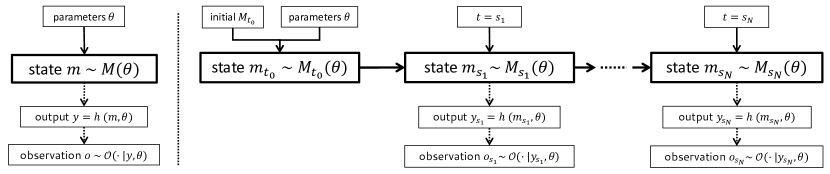
Figure 1: Scheme of a generic model (left) and a hidden-Markov model (right), mapping parameters $\theta$ to the state $m$, output $y$ and observation $o$ of the model $M$.

In a generic model $M$, a set of model parameters within a vector $\theta$ is mapped to the model "prediction", as depicted in the left part of Figure 1. We further categorize such model prediction into the full model "state" $m=M(\theta)$, and its hidden part (defined by function $h$, for instance, extracting only surface values from a three-dimensional lake model or accummulating only the number of adult individuals in an ecological community) as model "output" $y=h(m,\theta)$. If the model $M$ is stochastic (e.g. driven by a stochastic process and hence attaining a non-unique state $m$) then, given a suitable probability measure (denoted by $\mathbb{P}$), its state is characterized by a probability distribution $m\sim M(\theta)$, as a shorthand notation for state $m$ having a probability $\mathbb{P}(m|\theta,M)$. The ensemble of all possible "predictions" of such stochastic models are sometimes also referred to as "trajectories".

Many realistic models have an explicit temporal dimension (denoted in this manuscript by time $t$) as depicted in the right part of Figure 1. In such case, for each time $t$, we denote the model by $M_{t}$, a specific model state by $m_{t}$, and the model output as $y_{t}=h(m_{t},\theta)$. A stochastic time-dependent model $M$ is called a hidden-Markov model, if, for any increasing sequence of times $s_{1}<\dots<s_{N}$, its corresponding states $m_{t}\sim M_{t}(\theta)$ (but not necessarily its outputs $y_{t}$) satisfy the Markov property for all $\theta$ and all $1\leq k\leq N$:

$$\mathbb{P}(m_{s_{k}}|m_{s_{k-1}},\dots,m_{s_{1}},\theta,M)=\mathbb{P}(m_{s_{k}}|m_{s_{k-1}},\theta,M).$$ (1)

In a realistic scenario (to be modeled by model $M$), the value of the output $y$, which we could refert to as the "exact" or "true" output, is often not measured completely accurately during the observation process (independentent of a chosen model type). In particular, the corresponding data "observations" $o$ (see Figure 1) are instead assumed to follow a probabilistic distribution ${\mathcal{O}}(\cdot|y,\theta)$, sometimes referred to as the observational error model, potentially also depending on some uncertain parameters, included within the same vector $\theta$ for simplicity and brevity of the exposition.

For time-dependent models, the corresponding data observations $o_{t}$ at "snapshots" $t=s_{1},\dots,s_{\bar{N}}$ are assumed to be mutually independent and each follow a given ${\mathcal{O}}(\cdot|y_{s_{n}},\theta)$ distribution. Consequently, the entire observation sequence $(o_{s_{1}},\dots,o_{s_{N}})$ follows a tensorized distribution with a shorthand notation ${\mathcal{O}}(\cdot|y,\theta)=\otimes_{n=1}^{N}{\mathcal{O}}(\cdot|y_{s_{n}},\theta)$. In the following we refer to the observational error model simply by "error".

Finally, hierarchical Bayesian networks (as examples of "static" probabilistic models introduced in section 1) are supported as distributions (see subsection 5.6) for observational error and priors of model parameters and intial model states (see subsection 2.2), are hence are not incorporated among the "model" concept whithin manuscript.

2.2 Bayesian inference

Bayesian inference [GCS⁺14] can be used for statistical quantification (including uncertainties) of model parameters and (past, present and future) model states by conditioning the corresponding prior distributions on the data to get the corresponding posterior distributions. In particular, for a given model $M$ mapping the parameters vector $\theta$ to (possibly probabilistic) model state $m\sim M(\theta)$, the so-called likelihood $L(D|\theta,M)=\mathbb{P}(D|\theta,M)$ of the model $M$ defines a probability distribution of observations $D$ for given model parameter values $\theta$. In addition to the likelihood, initial information about parameters $\theta$ is described probabilistically by the so-called prior distribution $\pi(\theta|M)=\mathbb{P}(\theta|M)$. This prior knowledge on the model and its parameters is combined with the observed data $D$ via the likelihood $L(D|\theta,M)$ to obtain the posterior distribution $\mathbb{P}(\theta|D,M)$ of model parameters $\theta$:

$$\mathbb{P}(\theta|D,M)=\frac{L(D|\theta,M)\pi(\theta|M)}{\mathbb{P}(D|M)}\propto L(D|\theta,M)\pi(\theta|M),$$ (2)

where the Bayesian model evidence term $\mathbb{P}(D|M)$, useful for model selection, is independent of the parameters $\theta$.

For a deterministic model $M$, model output $y=h(m,\theta)=h(M(\theta),\theta)$ can be obtained for any arbitrary $\theta$, and hence the likelihood can be evaluated explicitly by applying the error, i.e. $L(D|\theta,M)={\mathcal{O}}(D|y,\theta)$. In addition to the posterior distribution $\mathbb{P}(\theta|D,M)$ of model parameters $\theta$ given by (2), the posterior distribution $\mathbb{P}(m|D,M)$ of model states $m$ is given directly by propagating $\mathbb{P}(\theta|D,M)$ through model $M$ using the procedures described in later sections.

For a stochastic model $M$, a conditional (on $\theta$) prior distribution $\pi(m|\theta,M)$ of the model states $m$ is also required (for simplicity, the same notation $\pi$ is used for the prior distributions of model parameters $\theta$ and of model states $m$). For instance, in a time-dependent stochastic model with state $m_{t}\sim M_{t}(\theta)$, a prior distribution $M_{t_{0}}(\theta)$ of the initial model state $m_{t_{0}}$ needs to be specified (possibly conditional on $\theta$), and then the prior distribution of the later model states $m_{t}$ at $t>t_{0}$ is determined by propagating $M_{t_{0}}(\theta)$ through model $M$. Given $\pi(m|\theta,M)$, the conditional (on $\theta$) posterior distribution $\mathbb{P}(m|\theta,D,M)$ of the (stochastic) model state $m$ can be inferred jointly with the posterior distribution $\mathbb{P}(\theta|D,M)$ of model parameters $\theta$ by evaluating their joint posterior $\mathbb{P}(\theta,m|D,M)$:

$$\mathbb{P}(\theta,m|D,M)=\frac{\mathbb{P}(D|\theta,m,M)\pi(\theta,m|M)}{\mathbb{P}(D|M)}\propto\mathbb{P}(D|\theta,m,M)\pi(\theta|M)\pi(m|\theta,M).$$ (3)

Note, that marginalization of (3) over stochastic model states $m$ recovers (2), where the evaluation of the likelihood $L(D|\theta,M)$ entails a marginalization over all possible model states $m\sim M(\theta)$:

$$L(D|\theta,M)=\int\mathbb{P}(D|\theta,m,M)\pi(m|\theta,M)dm.$$ (4)

In the remaining of this manuscript the dependence of $L(D|\theta,M)$ on prior model states distribution $\pi(m|\theta,M)$ will be understood implicitly via the dependency on model $M$ which is assumed to provide a prior distribution $M_{t_{0}}(\theta)$ for the initial model state $m_{t_{0}}$. The information of the prior distribution for later model states $\pi(m_{t>t_{0}}|\theta,M)$ is usually incorporated as a specific evolution structure within the model $M$ and hence is also implicitly taken into account as a dependency for likelihood $L(D|\theta,M)$.

2.3 Numerical methods for Bayesian inference

Usually, Bayesian inference cannot be solved analytically for posteriors $\mathbb{P}(\theta|D,M)$, and in the case of stochastic model $M$, usually not even for likelihood $L(D|\theta,M)$ in Equation 4 and hence also not for posterior of model states $\mathbb{P}(m|D,M)$. Therefore, numerical methodologies have been developed to sample from the posterior distribution of model parameters $\theta$ (and states $m$, if the model is stochastic), obtained by running numerous corresponding simulations of the model $M$. Existing non-intrusive methods include the Metropolis or Metropolis-Hastings Markov chain Monte Carlo (Markov-type for short) [GL06, GCS⁺14, Has70, MRRT53], Gibbs-type samplers for modifying one parameter at a time [RM09], and the Approximate Bayesian Computation (ABC-type for short) [AKS15]. Alterantive partially intrusive (but usually faster) methods include Hamiltonian Monte Carlo (HMC-type for short) and Variational Bayesian Inference (SVI-type for short), based on exact analytical solution to an approximation of the posterior. Sampling of posterior model states $m$ in stochastic models can be achieved, for instance, using Conditional Ornstein-Uhlenbeck Sampling COUS [RM09] within Gibbs-type samplers, Particle Filtering [ADH10] within Markov-type samplers, or by recasting model $M$ to consider all its states $m$ as parameters as well [AUS16] in HMC. ABC-type methods require minimal model structure restrictions and are able to reliably sample from model parameters posterior $\mathbb{P}(\theta,|D,M)$, but are often very inefficient in sampling posterior of model states $\mathbb{P}(m|\theta,D,M)$, since the high-dimensional model output $y$ is usually compressed to a low-dimensional sufficient summary statistic $\mathcal{S}(y)$. HMC and Variational Inference methodologies usually have the best performance, but are intrusive (problem reformulations and/or derivatives are required). Next, we briefly describe Markov-type and ABC-type samplers, depicted by simplified algorithm flowcharts in Figure 2 and already available within the SPUX framework.

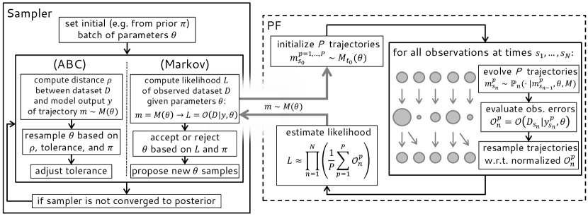
Figure 2: Left: a simplified flowchart of the numerical posterior sampling algorithms of the Markov- and ABC-types. Right: a simplified flowchart of the Particle Filter (PF) algorithm sampling posterior trajectories (states) of a stachastic model by filtering them w.r.t. dataset and the observation error model and estimating the likelihood defined as an integral in Equation 4. Note, that ABC-type samplers estimate posterior of model parameters (but not states).

2.3.1 Markov-type sampling

In the Markov-type sampling, samples from the posterior distribution of model parameters are generated iteratively. In each iteration, model parameters are proposed, for which the prior and the likelihood are evaluated (up to an arbitrary factor) by considering model output (if needed). These are then either accepted or rejected (in the latter case, the parameters from the previoius step are kept). Acceptance or rejection is based on the ratio of current and previous posterior density estimates (i.e. the product of likelihood and prior as evinced from Bayes theorem). In the ABC-type sampling, the initial set of model parameters is drawn from the prior distribution. Then, an iterative procedure consist of multiple tolerance steps (converging to zero), evaluating the distance metric between the model output and the observations (data), re-drawing a subset of the model parameters and accepting part of them based on the distance and the adjusted tolerance, this way gradually tuning the initial prior model parameter samples to the posterior model parameter samples.

2.3.2 Posterior trajectories sampling and likelihood estimation for stochastic models

For stochastic models, in addition to posterior distribution of the model parameters $\theta$, sampling of the posterior distribution of model states $m$ is also required. In particular, the estimation of the (marginalized) likelihood (4) required in the Markov-type samplers is most often estimated numerically. Nonlinear filtering numerical schemes, such as Particle Filter (PF) with or without smoothing (also known as Particle Markov Chain Monte Carlo (PMCMC) technique [ADH10]) or a (Seamless) multi-level (Ensemble Transform) Particle Filter ((S)ML(ET)PF) [GC17] can be employed. Any Markov-type sampler can be combined with the (ML)PF method for likelihood estimations, where the hidden-Markov structure of the underlying stochastic model $M_{t}$ is exploited for efficient marginal likelihood approximations using time-series observations [ADH10, KR17]. In particular, for observations $D$ consisting of time-series data $D=\{D_{s_{n}}:n=1,\dots,N\}$ at time snapshots $t=s_{1},\dots,s_{N}$, the marginal likelihood in (4) can be rewritten (using the Markov structure, see [KR17]) as

$$L(D|\theta,M)=\int\pi\left(m_{s_{0}}|\theta,M\right)\prod_{n=1}^{N}\mathbb{P}_{n}\left(m_{s_{n}}|m_{s_{n-1}},\theta,M\right){\mathcal{O}}(D_{s_{n}}|y_{s_{n}},\theta)dm_{s_{0}}\dots dm_{s_{n}}.$$ (5)

Here, for given parameters $\theta$, probability distributions $\mathbb{P}_{n}(m_{s_{n}}|m_{s_{n-1}},\theta)$ characterize random model state vector $m_{s_{n}}$ given previous state $m_{s_{n-1}}$, representing propagation of a given model state $m_{s_{n-1}}$ to the next state $m_{s_{n}}$, The observational likelihood is evaluated using the (abbreviated) error ${\mathcal{O}}_{n}(D|y,\theta)={\mathcal{O}}(D_{s_{n}}|y_{s_{n}},\theta)$ for model output $y_{s_{n}}=h(m_{s_{n}},\theta)$ and provides a probabilistic model for the data observation process [KR17]. The PMCMC algorithm [ADH10, KR17] uses PF to provide an unbiased statistical estimate of the proposal parameter marginal likelihood $L(D|\theta,M)$ with structure given in equation 5. As depicted in Figure 2 (right), the numeric approximation of equation 5 involves sampling model trajectories ("particles") in terms of model states $m^{p}$ (with $p=1,\dots,P$) of the underlying model $M$ with parameters $\theta$. At each measurement time $s_{n}$ in the observations time series, model simulations are paused and all particles are re-sampled (bootstrapped) according to their (abbreviated) observational likelihoods ${\mathcal{O}}_{n}^{p}(D|\theta)={\mathcal{O}}_{n}(D|y^{p},\theta)$ with $y_{s_{n}}^{p}=h(m_{s_{n}}^{p},\theta)$. Such periodic re-sampling increases algorithmic complexity due to the required destruction and replication of existing particles, however, provides an efficient way of sampling "intermediate" posterior model states (i.e. $\mathbb{P}(m_{s_{n}}|\theta,D_{s_{1},\dots,s_{n}},M)$ conditioned only on the partial dataset $D_{s_{1},\dots,s_{n}}$ up to the filtering time $s_{n}$). At the end of the PF, an unbiased estimate $\hat{L}(D|\theta,M)$ of marginal likelihood $L(D|\theta,M)$ as in equation 5 is evaluated by

$$L(D|\theta,M)\approx\hat{L}(D|\theta,M)=\prod_{n=1}^{N}\left(\frac{1}{P}\sum_{p=1}^{P}{\mathcal{O}}^{p}_{n}(D|y,\theta)\right)=\prod_{n=1}^{N}\left(\frac{1}{P}\sum_{p=1}^{P}{\mathcal{O}}(D_{s_{n}}|y^{p}_{s_{n}},\theta)\right).$$ (6)

In implementation, the evaluation fo $\hat{L}(D|\theta,M)$ is performed in log-scale to mitigate numerical roundoff errors. The accuracy (namely, the variance) of the PF likelihood estimate clearly depends on the number of used particles $P$. At the initial burn-in stage, the sampling acceptace procedure is often dominated by the low likelihood values and hence the inaccuracy of the PF estimator is of secondary importance. However, when sampler is converged towards the posterior, a larger number of particles is prefered to ensure low relative approximation error in likelihood estimator. In supplementary Appendix G, we describe an adaptive procedure to automatically set the number of particles throughout the sampling procedure based on the feedback containing historical estimator accuracies and parameters fitness. To guarantee the convergence of the posterior, the particle adaptivity is "locked" after the specified period of sampling, which should be smaller or equal to the burn-in phase.

Additional methodologies, often refered to by "smoothing" [DJ09], are often employed to obtain "smoothed" trajectories (conditioned on the entire dataset $D$) from posterior model states $\mathbb{P}(m|\theta,D,M)$. One way to achieve this is to resample already available "intermediate" posterior trajectories (conditioned only on the partial dataset $D_{s_{1},\dots,s_{n}}$). In particular, a simple yet very computationally efficient (w.r.t. to both runtime and memory usage) "rejection" based smoothing (see sections 2.3 and 5 [DJ09] and [JMR15]) sequentially iterates $s_{n}$ from $s_{1}$ to $s_{N}$ to generate trajectories from posteriors $\mathbb{P}(m_{s_{1}},\dots,m_{s_{n}}|\theta,D_{s_{1},\dots,s_{n}},M)$ by an additional re-filtering step (after the main PF filter step only for $s_{n}$) for all preceeding snapshots $s_{1},\dots,s_{n-1}$ as well. Note, that such "rejection" smoothing, unlike the PF filter for likelihood estimation, is prone to particle degeneracy (i.e. collapses to a single trajectory for each sample of posterior parameter $\theta$) for $n\ll N$ [DJ09] and hence should be used with care for non-illustrative purposes. More sophisticated (but also more computationally expensive) techniques to prevent such particle degeneracy have been also reviewed in [DJ09].

2.3.3 Approximate Bayesian Computation

If the model $M$ does not have a hidden-Markov structure, or if the error ${\mathcal{O}}(\cdot|y,\theta)$ is not explicitly available as a probabilistic distribution (i.e. only a direct sampling of $o=y=h(m,\theta)$ by sampling $m$ from a probabilistic distribution $M(\theta)$ is possible), then the efficient numerical likelihood estimation methods from subsubsection 2.3.2 cannot be directly applied. Note, that if data $D$ consists only of a single observation, there are obviously no efficiency gains in using the (temporally) adaptive likelihood estimation using Particle Filtering.

In such cases, a more general (but potentially less efficient due to the lack of adaptive temporal filtering) Approximate Bayesian Computation (ABC) methodology [AKS15] can be used to sample from the posterior distribution, without requiring the evaluation of the likelihood as in Equation 4. In particular, in Boltzmann-type ABC methods, the joint posterior of model parameters and states is approximated by the following family of distributions

$$\mathbb{P}_{\tau}(\theta,m|D,M)=\frac{1}{Z(\tau)}L(o|\theta,M)\pi(\theta|M)e^{-\frac{\rho(D,o)}{\tau}}\quad\text{where}\quad o\sim{\mathcal{O}}(\cdot|y,\theta),\quad y=h(m,\theta)$$ (7)

and where $1/Z(\tau)$ is a normalization factor, $\tau$ is the selected tolerance level, and $\rho(D,o)$ measures how close the observational dataset $D$ is to the model observation $o$. If the error ${\mathcal{O}}$ is not available explicitly, $o=y=h(m,\theta)$ is used instead. Given distance $\rho$, an initial tolerance level $\tau_{0}$, and an initial distribution (usually prior $\pi(\theta|M)$), ABC-type samplers use a sequence of tolerances $\tau_{i}\to 0$ to generate a sequence of approximations to $\mathbb{P}(\theta,m|D,M)$. In the following, dependencies of a particular distance value $\rho(D,o)$ on the parameters $\theta$ and the model $M$ (and, if available, also of the error ${\mathcal{O}}$) are explicitly represented by using a supplementary notation $\rho(D|\theta,M)$ for $\rho(D,o)$ with a realization for $o$ obtained from $\theta$ and $M$ as described above.

2.4 Uncertainty propagation and forecasting

For time-dependent models $M(\theta)=M_{t}(\theta)$, once the joint posterior distribution $\mathbb{P}(\theta,m_{[t_{0},T]}(\theta)|D,M)$ of model parameters and states (up to the last snapshot time $T=s_{N}$) is available, the distribution of the "future" (forecast) model states $\mathbb{P}(m_{[T,\infty)}(\theta)|D,M)$ is given by propagating $\mathbb{P}(\theta,m_{T}(\theta)|D,M)$ to the "future" times $t>T$ using the model $M$. In practice, this is achieved with a Monte Carlo (MC) sampler, where samples from $\mathbb{P}(m_{[T,T_{F}]}|\theta,D,M)$ are obtained by sampling from $\mathbb{P}(m_{T}|\theta,D,M)$ and propagating them for $t\in[T,T_{F}]$ for some future time $T_{F}>T$.

Such an MC sampler can also be used for somewhat less difficult direct propagation of uncertainty from prior distributions, when dataset is not available. For very challenging priors, Markov-type samplers from subsubsection 2.3.1 can be employed by using prior density instead of the likelihood.

3 SPUX framework

In this section we introduce the SPUX framework, focusing on the purpose and design specification in subsection 3.1, available modular components and built-in services in subsection 3.2, and parallelization capabilities in subsection 3.3. A collection of continously updated current and past examples of SPUX applications is illustrated at the end, in subsection 3.4.

3.1 SPUX purpose and design specification

The purpose of the SPUX framework is to provide a seamless high-level interface to perform Bayesian inference with a free choice of methodologies, algorithms, and computational environments. To achieve such flexible customization and effortless adaptivity, the SPUX framework harnesses the powerful dynamic typing and runtime polymorphism offered by the modern Python programming language, which has recently become one of the most popular programming languages for scientific computing. In essence, the SPUX framework is a collection of carefully selected, designed and optimized modular components. The modularity of SPUX components extends beyond the conventional restrictive patterns and instead follows a "duck typing" design philosophy [duc18], namely, the suitability of an object to perform a function is not determined by the object’s type, rather by the support of certain methods and properties by the object itself. An overview of the basic key components currently implemented in SPUX, each with the purpose of representing a particular mathematical concept as introduced in section 2, together with available specific numerical methods for each component type, is provided in the table below:

Concept	Component	Numerical method / algorithm	Description
$\mathbb{P}(\theta,m|D,M)$	Sampler	EMCEE, SABC, MCMC, MC	parameters sampling
$L(D|\theta,M)$	Likelihood	Direct, PF	states sampling and likelihood
$\rho(D|\theta,M)$	Distance	Norm, Regression	distance for ABC sampler
$m_{t}\sim M_{t}(\theta)$	Model	Randomwalk, External, …	model for user’s application
$\Pi(\cdot),\Sigma(\cdot)$, etc.	Aggregator	Trajectories, Replicates	aggregator of components

3.2 SPUX component assignments and built-in services

All available SPUX components can be assigned to each other following the required dependencies. An example scheme for such assignment of the components required by any Markov-type sampling algorithm for Bayesian inference is provided in Figure 3 (the left part), together with the associated mathematical objects introduced in section 2. The right part of this same scheme depicts an assignment of the components together with the associated mathematical objects for the a posteriori forecast stage, introduced in subsection 2.4.

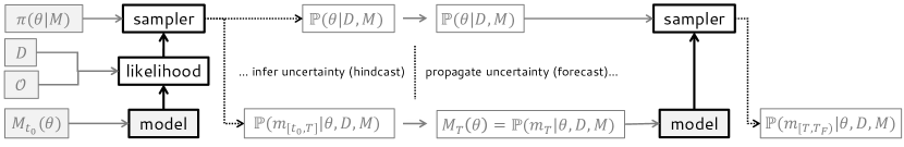
Figure 3: Component assignment and execution flow scheme for the SPUX framework using Markov-type sampler and likelihood components for the inferenece (hindcast up to the last time $T$ in dataset $D$) and the resulting bootstrapped posterior parameters and model states distributions for the forecast (uncertainty propagation beyond the last time $T$ in dataset $D$). Boxes with thin outlines indicate the associated mathematical objects introduced in section 2, and boxes with thick outlines and thick arrows indicate SPUX components and their internal assignments, respectively. Thin solid and dotted arrows represent component inputs and outputs, respectively. White background indicates built-in components and inference outputs, whereas gray background indicates anticipated framework inputs.

Each SPUX component (for both stages: hindcast and forecast) is described in detail in section 4. Such modularity in SPUX allows easy implementation of different numerical approaches for Bayesian inference. For instance, subsection 5.12 explain how to use a structurally different ABC-type method (see subsubsection 2.3.3) within SPUX.

3.3 SPUX parallelization capabilities

One of the key advantage of SPUX is its very transparent yet very flexible parallelization sub-system. In particular, multiple parallel workers can be attached to each spux component listed in subsection 3.2 and depicted in Figure 3. An example of such parallelization scheme with only three components (sampler, likelihood, and model) is provided in Figure 4, where sampler samples, likelihood particles, and multiple tasks of the (optionally) parallel user’s application/model (more details in subsection 5.10) are distributed over available attached workers. Additional parallel components can be incorporated when needed; for instance, the Replicates aggregator is designed to assimilate multiple independent observational data sources in parallel. Note, that neither the model (i.e. the associated user’s application) nor any other SPUX component is strictly required to be parallelized; instead, any of these components might also be serial (i.e. without any parallel workers attached).

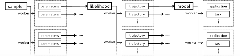
Figure 4: An example of parallelization capabilities for various compontents of the SPUX framework described in subsection 3.2 and depicted in Figure 5. Three levels of hierarchical parallelization are used here: parallelization over multiple model parameters samples of the EMCEE sampler, over multiple particles of the PF likelihood, and over multiple independent tasks of a parallel user’s application. For each SPUX component (depicted using thick lines), the thin solid arrows represent the required (possibly independent) tasks to be executed, the thick solid arrows represent the internally called methods, and the dotted lines represent the remaining ommited parts of the scheme.

For a more detailed description of parallel hierarchically stackable SPUX executors, refer to the technical section 6.

3.4 SPUX gallery

Inspired by the "Demo Data as Code" concept [Lim19], SPUX documentation website hosts a gallery listing examples of user’s applications, including source codes, authors, scientific fields, model programming languages, used computational environment and configuration, figures with representative results, and associated scientific publications. At the time of this writing, example fields include hydrology, aquatic ecology, urban hydrology, limnology, physics and data science, but the generality of the SPUX framework does certainly extend beyond. In particular, SPUX is currently being actively used for Bayesian inference in realistic individual-based modelling of riverine macro invertebrates,time-dependent conceptual hydrological modeling of catchments,stochastic-input driven hydrological modeling of the rainfall runoff systems,and high resolution three-dimensional hydrological (and, eventually, ecological) operational modeling of Lake Geneva.

4 SPUX framework showcase with a random walk model

This section guides the reader through an example model and usage pattern of SPUX. An overview of different SPUX installation methods can be found on the SPUX documentation page, where we also provide the links to access the source code, and a pre-configured SPUX Jupyter notebook (offered on a best-effort basis only). After a brief overview of model types in subsection 4.1, an example model of a random walk and its setup in SPUX are described in subsection 4.2. The serial model execution procedure with a brief overview of resuts is described in subsection 4.3. In subsection 4.4, minor auxiliary setup and execution steps needed to run SPUX in parallel on workstations and high performance clusters are addressed. A detailed automatic PDF report compiling inference setup, results, diagnostics and performance is introduced and interpreted in subsection 4.5. Finally, subsection 4.6 and subsection 4.7 describe procedures building upon already estimated posteriors for model parameters and states: re-executing the best (or any other) model trajectory and forecasting to future times or performing sequential Bayesian updating for a new dataset.

4.1 Deterministic and stochastic models

SPUX supports all types of models for Bayesian inference introduced in section 2: deterministic, where model evaluation is uniquely determined by parameters $\theta$, and stochastic, where model state depends on random variable(s) (e.g. initial data) and/or is driven by stochastic process(es).

In Bayesian inference for deterministic models $M$, a simple Direct likelihood can be analytically computed using the specified error: $L(D|\theta,M)={\mathcal{O}}(D|y,\theta)$ with $y=h(m,\theta)$ and $m=M(\theta)$. An example of such model, Straightwalk, is available at examples/straightwalk.

For stochastic models $M$, in addition to uncertain model parameters $\theta$, also the uncertain model states $m\sim M(\theta)$ need to be inferred. In such cases, the error ${\mathcal{O}}(D|y,\theta)$ by itself is often not sufficient to analytically compute the likelihood $L(D|\theta,M)$ in (4) for given model parameters. Hence, additional approximation techniques are required, as discussed in section 2. An example of a stochastic time-independent model (left part of Figure 3) is provided in examples/gaussian-sabc. Another built-in model in SPUX is a stochastic version of the Straightwalk model, called Randomwalk, where the direction and size of each (time) step of the walker is a random variable. Since the SPUX framework is tailored to Bayesian inference with stochastic time-dependent models, in the following section we showcase the Randomwalk model. Files mentioned throughout next section are located in SPUX repository at examples/randomwalk (assumed to be the current working directory).

4.2 Randomwalk model

The Randomwalk model describes a stochastic walk on a line (i.e. a set of real numbers). Its goal is to provide the simplest possible conceptual model, which has just enough complexity to illustrate most of the functionality in SPUX, while addressing the majority of requirements in the environmental scientific modeling. Given a prescribed time step size $\Delta t$ (in seconds for example, to fix the ideas) as a numerical discretization parameter, together with an initial time $t_{0}$ and an initial (possibly uncertain) position $m_{t_{0}}\sim M_{t_{0}}$ [m], the model iteratively takes random steps on a one-dimensional line every $\Delta t$ time units. The direction and the size of each step depend on the time step size, on two models parameters, the drift $\mu$ [m/s] and the volatility $\sigma$ [$ms^{-1/2}$], and on an independent standard normal random variable ${\mathcal{N}}_{t}$:

$$m_{t+\Delta t}\sim\mathbb{P}(m_{t+\Delta t}|m_{t})=m_{t}+\Delta t\mu+\sqrt{\Delta t}\sigma{\mathcal{N}}_{t}.$$ (8)

The Randomwalk model is a built-in SPUX model class with model initialization and evolution (according to (8)) implemented in the corresponding class methods:

init(...)	initialize model with initial state $m_{t_{0}}$ and model parameters $\theta$
run(...)	run model up to the specified time $t$ and return model prediction output $y_{t}$

For implementation details of this demonstrational model, focused on simplicity and code readability (no vectorization, explicit for-loops), refer to 12 in Appendix D. In this particular model, the initial argument contains the initial time $t_{0}$ and the initial position $m_{t_{0}}$. Alternatively, initial contents might as well be assigned in the model constructor directly, as for the time step size $\Delta t$. However, such explicit specification of the model input (i.e., using initial) at the initialization provides more flexibility in the cases where the initial position $M_{t_{0}}$ is uncertain (see subsection 4.3) and/or when multiple observational datasets are available (see subsection 5.9). Finally, we assume $h(m,\theta)=m$, i.e. model state coincides with the model output.

4.3 Inference for Randomwalk model

As briefly described in subsection 3.2, all available SPUX components can be assigned among each other following the required dependencies. An extended version of the assignment scheme in Figure 3 for this example, together with the associated mathematical objects introduced in section 2, is provided in Figure 5. The final assigment assigns the top component, in this case (and also usually) the sampler, to the built-in main SPUX framework component. The SPUX framework component provides the hierarchical sandboxing (isolation to dedicated directories) and seeding (controlling the independence of random number streams and ensuring reproducibility independently of the chosen computational environment), manages runtime checkpointing, diagnostics, and framework setup options (see later subsection 5.1).

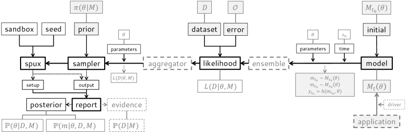
Figure 5: Component assignment and execution flow scheme for the SPUX framework using Markov-type sampler and likelihood components (an extension of the summary Figure 3). Boxes with thin outlines indicate the associated mathematical objects introduced in section 2, and boxes with thick outlines and thick arrows indicate SPUX components and their assignments for internal evaluation, respectively. For each SPUX component, thin solid and dotted arrows represent component inputs and outputs, repspectively. White background indicates built-in components and inference outputs, whereas gray background indicates anticipated framework inputs. Dashed boxes indicate optional SPUX components for special sampler, likelihood, model or dataset requirements and optional output or reporting capabilities.

In the following subsections we provide an elaborate description of the remaining SPUX framework prerequisites, supplementary capabilities, and a general inference execution workflow, using the Randomwalk model (introduced in subsection 4.2) as the underlying example.

4.3.1 SPUX configuration prerequisites

To perform Bayesian inference for the given model, we also need to specify several configuration files for the remaining essential prerequisites (besides the sampler, the likelihood and the model). In particular, for the Randomwalk example, these prerequisites are: the available observational data $D$, a statistical error ${\mathcal{O}}(D|M(\theta),\theta)$, prior distributions $\pi(\theta|M)$ for all the parameters that we intend to infer, and the initial model state $M_{t_{0}}(\theta)$. Note, that the parameters $\theta$ contain both the parameters of the model $M$ and, if present, the hyper-parameters used for constructing the distributions of the error ${\mathcal{O}}(\cdot|y_{s},\theta)$ and/or of the initial model states $M_{t_{0}}(\theta)$. Prior initial model state distribution $M_{t_{0}}(\theta)$ is then attached to the specified model component (representing $M(\theta)$), error ${\mathcal{O}}(D|M(\theta),\theta)$ is attached to likelihood component (representing $L(D|\theta,M)$), and prior model parameters distribution $\pi(\theta|M)$ is attached to sampler component (representing $\mathbb{P}(\theta,m|D,M)$), see subsection 3.2 and Figure 5.

Marginal prior distributions $\pi_{\mu}$, $\pi_{\sigma}$, $\pi_{\varepsilon}$ for each parameter $\theta=(\mu,\sigma,\varepsilon)$ of the joint prior distribution $\pi(\theta|M)$, with $\varepsilon$ being the standard deviation (as a hyper-parameter) of the (assumed) Gaussian error (described below), are assumed to be independent and are given by (for plots, refer to Figure 6):

$$\pi_{\mu}={\mathcal{U}}(-1,1)\ [m/s],\quad\pi_{\sigma}={\mathcal{U}}(5,15)\ [ms^{-1/2}],\quad\pi_{\varepsilon}={\mathcal{L}}{\mathcal{N}}(1,1)\ [m].$$ (9)

This multivariate prior distribution is defined in prior.py using a built-in Tensor SPUX distribution (see subsection 5.6 for an overview of all SPUX distributions). The Tensor combines multiple statistically independent distributions (provided as a Python dictionary of the corresponding univariate distributions - for instance, from the scipy.stats package) to a multivariate SPUX distribution. The initial position $m_{t_{0}}$ of the randomwalk is also uncertain, and hence a prior distribution $M_{t_{0}}$ for the initial position $m_{t_{0}}$ at (deterministic) time $t_{0}=0$ is defined in initial.py:

$$m_{t_{0}}\sim M_{t_{0}}(\theta)={\mathcal{N}}(10,2)\ [m],\quad t_{0}\sim\delta_{0}\ [s].$$ (10)

We note, that $m_{t_{0}}$ could alternatively be included as a model parameter in the prior defined in (9).

Actual dataset files are located in the datasets directory. The default container for dataset management in SPUX is a DataFrame of the pandas package [McK10], which is very similar to the dataframe in the R programming language. The example script to load the dataset into a DataFrame, is located in dataset.py. The dataset provides inaccurate observations $D_{s}$ of the position $m_{s}$ at (snapshot) times $s=s_{1},\dots,s_{N}$. N/A values are allowed, however, no column (quantity of interest) or row (snapshot) should contain only N/A values.

The inaccuracies in observational data are modeled with an error, which is a statistical distribution of the observations (from the dataset) conditional on the specified model output prediction (from the simulation). In this example this distribution is assumed to be normally distributed with mean equal to the position $m_{s}$ predicted by the model, and with standard deviation given by an additional uncertain parameter $\varepsilon$ used as a hyper-parameter:

$$D_{s}\sim{\mathcal{O}}(\cdot|y_{s},\theta)={\mathcal{N}}(y_{s},\varepsilon)\ [m].$$ (11)

All observations are assumed to be statistically independent. The observational error is defined in error.py as a function (or a collable object) which, given the model output prediction and parameters, constructs the statistical distribution above as a SPUX Distribution instance.

An (optional) dictionary specifying units (as LaTeX-supported strings) for each parameter, model output and time dimension is specified in units.py. Its contents are used only in the SPUX report.

Within the context of this illustrative example, we also make use of the (optional) exact (loaded in exact.py) parameter values available at datasets/exact.dat and the exact (synthetic) model outputs (without the observational noise) available at datasets/predictions.dat.

4.3.2 SPUX configuration and execution - user interface (UI)

The quickest way to run SPUX inference and post-processing (discussed in the following sections) is using the SPUX UI configuration file spux.cfg. There, arguments required for the construction, configuration, initialization, and execution of each SPUX component (either built-in or manually imported) can be specified, including any prerequisite script (see subsubsection 4.3.1) defining required (mandatory or optional) options. All such components and options can be configured as depicted in 1, where an adaptive Particle Filter (PF with the default "rejection" smoothing) likelihood with the specified maximum number of particles is assigned to an Affine Invariant Ensemble sampler (EMCEE) with the specified number of concurrent chains. Additional framework options (i.e. not specific to any component) can also be specified in spux.cfg to control various aspects of the SPUX framework, as depicted in 2. For instance, optional units of time, model parameters and observations can be specified (see also subsection 5.6). Built-in component and framework options are described throughout the following sections with a summary available in subsection 5.1.

Listing 1: Example spux.cfg for components

⬇

model Randomwalk

model.dt 0.1

likelihood PF

likelihood.particles 256

sampler EMCEE

sampler.chains 32

sampler.samples 10000

Listing 2: Additional options in spux.cfg

⬇

prior prior.py

error error.py

dataset dataset.py

initial initial.py

burnin "half"

units units.py

exact exact.py

Using SPUX UI, inference and post-processing can be setup and performed by simply executing:

spux spux.cfg --execute --all

This automatically generates the required SPUX scripts (described in the following sections) and automatically executes testing, synthesis, inference, reporting, and re-execution of the best trajectory.

The inference process can be terminated at any time, since the output is periodically checkpointed (see subsection 5.1). Additional runtime arguments can be specified to customize the inference:

--dry	"dry run" mode - inspect configuration without actual sampling
--continue	continue the inference process starting from the latest checkpoint
--no-repro	disable reproducibility information (stored in randomwalk_reprozip.rpz)

The list of all built-in components and options is also retrievable by executing spux --help.

4.3.3 SPUX configuration and execution - application programming interface (API)

The most flexible way to configure SPUX is to use a configuration script in which the prior, error model, and dataset are explicitely imported and assigned (using the SPUX API) to the selected SPUX components, such as likelihood (or distance) and sampler. A summary of an example configure.py (excluding trivial module imports) is provided in 3. The mandatory spux.assign(...) assigns all hierarchically ordered components to the SPUX framework.

Listing 3: Example configure.py (excluding imports)

⬇

model = Randomwalk (dt=0.1)

model.configure (initial)

likelihood = PF (particles=256)

likelihood.configure (dataset, error)

sampler = EMCEE (chains=32)

samper.configure (prior, samples=10000)

spux.configure (units)

spux.assign (model, likelihood, sampler)

Listing 4: Example infer.py

⬇

from configure import *

spux.setup ()

spux.init ()

sampler.init ()

sampler ()

spux.exit ()

The execution script infer.py provided in 4 imports the components from configure.py, setups the SPUX framework (mandatory spux.setup(...), see subsection 5.1), initializes the sampler (mandatory sampler.init(...) for EMCEE), and performs the posterior sampling of the model parameters and states for the specified number of samples. The mandatory framework initialization spux.init(...) and finalization spux.exit(...) methods manage the required computational resources. For the EMCEE sampler, initial model parameters are drawn by default from the specified prior. The script can be executed by typing python infer.py in the console. Analogously to the UI in subsubsection 4.3.2, the --dry, --continue and --no-repro runtime arguments can be used for infer.py to enable "dry mode", continuation or disable reproducibility package.

4.3.4 SPUX results

The estimated marginal posteriors of model parameters are provided in Figure 6 and the estimated marginal posteriors of model predictions are provided in Figure 7.

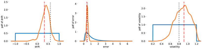
Figure 6: Marginal posterior (orange) and prior (blue) distributions of model parameters. The red dashed line indicates the best found parameters values. The black dotted line represents the exact parameter values.

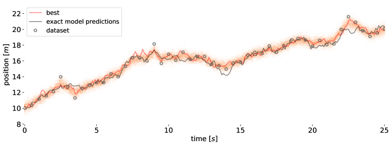
Figure 7: Posterior distribution of model predictions for the observational dataset. The shaded orange regions indicate the log-density of the posterior model predictions distribution at the respective time points, the red line represents the best found model prediction, the black line represents the exact model prediction values.

For the inference results, the default burnin period (half of all samples) was selected to remove the initial sampler bias. The adaptive number of particles described later in Appendix G is locked after the specified lock batches. By default the burnin is also set to this value to avoid any potential bias due to the adaptivity process. For post-processing, only every thin-th sample (of each sampler chain) is selected in order to obtain a sequence of statistically independent posterior samples. In particular, the default "auto" value was used for the thin period, which uses the median of optimal thinning periods obtained by estimating multivariate effective posterior sample sizes for each sampler chain.

4.4 Parallel inference for Randomwalk model

With minimal effort, the above example configuration can be parallelized either for a local machine or for a remote high performance computing (HPC) cluster. We emphasize, that no modifications are needed for this particular "Randomwalk" model class. For HPC cluster, consider placing (see subsection 5.1) the output directory in a parallel high performance "scratch" filesystem, if available. For a more detailed discussion regarding models not written in pure Python, refer to section 5.

4.4.1 Attaching parallel workers

To enable parallel execution, a required number of parallel workers can be attached to each SPUX component, as depicted in Figure 3. Examples are provided in 5 (for the UI configuration file spux.cfg as in 1) and in 6 (for the API inference script infer.py as in 4, in this case these lines should be placed before the calls to framework setup and initialization).

Listing 5: Parallel workers in spux.cfg.

⬇

likelihood.workers 8

sampler.workers 16

Listing 6: Parallel workers in infer.py.

⬇

likelihood.attach (workers=8)

sampler.attach (workers=16)

A separate dedicated core is used for the manager process of each group of parallel workers. For an advice regarding worker allocation strategies across multiple parallel executors, refer to Appendix B. Advanced explicit attaching of SPUX executors to components is described in subsection 6.1.

4.4.2 Launching parallel SPUX

Assuming a library for the Message Passing Interface (MPI) [Mes15] is installed, parallel scripts need to be launched through the Python mpi4py module. For the execution using the UI, specify --mpi runtime argument. For infer.py using the API:

mpiexec -n 1 python -m mpi4py infer.py.

The required worker MPI processes will be spawned automatically (i.e. according to the resources table).

For HPC systems not supporting dynamical spawning of new MPI processes, the required number of MPI ranks (workers) needs to be explicitly specified for mpiexec (after "-n"). The cumulative number of required workers is indicated in the bottom right cell of the computational resources table (see example in LABEL:R-t:randomwalk_environment), which is printed to the console already during the "dry run" mode (for which one core is sufficient, i.e. no MPI is required). For convenience (e.g. to automate parallel job submission process), this number is also written to the dedicated workers.txt file. Parallelization can be temporarily disabled with --serial runtime argument, which ignores all workers attachments. SPUX documentation outlines specifics regarding different MPI libraries and useful advice to address any potential issues.

4.5 SPUX report

All tables and figures generated by the SPUX framework, such as previous Figure 6 and Figure 7, are automatically included (see Appendix A for technical details) in a PDF report (A4 and "slides" layouts), described in later sections. Such PDF report is also provided to support this section on SPUX usage as Suplementary Material. All of the tables, figures, and even the configuration scripts (in LABEL:R-s:report-scripts) referenced within this section are available in this report, hence it is strongly advisable to have a separate copy of the Suplementary Material at hand. Additionally, the "reproducible package" spux.rpz is generated using the "reprozip" tool [CRSF16]. The SPUX report and the spux.rpz provide the highest level of reproducibility (excluding containerization techniques) for an inference or forecast run, independently of the chosen computational environment and/or hardware.

4.5.1 Configuration and setup section

SPUX configuration and setup is summarized in the first section of the SPUX report (see LABEL:R-s:report-setup), which is generated by executing the example report.py script and contains the following:

configuration	LABEL:R-t:randomwalk_configuration	SPUX configuration: component classes and their options
setup	LABEL:R-t:randomwalk_setup	framework options from spux.setup(...), see subsection 5.1
units	LABEL:R-t:randomwalk_units	units for parameters, observations, and time
exact	LABEL:R-t:randomwalk_exact	exact model parameters (if specified)
evaluations	LABEL:R-t:randomwalk_evaluations	total number of anticipated model evaluations across components
datasets	LABEL:R-f:randomwalk_datasets	dataset(s) $D$ and exact model predictions (if specified)
errors	LABEL:R-f:randomwalk_errors	marginal error models ${\mathcal{O}}$ distributions for the specified $\theta,y$
prior	LABEL:R-f:randomwalk_prior	marginal prior distributions of model parameters - $\pi(\theta,M)$
initials	LABEL:R-f:randomwalk_initials	marginal prior distributions of initial model states - $M_{t_{0}}(\theta)$

In particular, for the Randomwalk example, at most 256 particles were used in the PF likelihood (with adaptivity enabled, see Appendix G), and 32 chains were used in the EMCEE sampler. In total, 10’000 samples were requested, locking particle adaptivity after 75 sample batches (2’400 samples).

4.5.2 Results and diagnostics sections

To load and visualize inference results and diagnostics using the API, the report.py script is executed with the additional --results runtime argument. This report.py script uses built-in plotting routines available in spux.reports.mpl module. The user can freely choose to use the reconstructed results and diagnostics with other established data visualization libraries, including the specialized pandas.plotting module and arviz [KCHM19] package. The report script generates multiple tables and figures of the results and diagnostics, and updates the SPUX report accordingly.

The inference results tables and figures included in LABEL:R-s:report-results of the SPUX report provide posterior distributions for model parameters and predictions (i.e. model outputs $y$ or even model states $m$):

best-parameters	LABEL:R-t:randomwalk_best-parameters	best found (e.g. maximum a posteriori) model parameters
parameters	LABEL:R-f:randomwalk_parameters	marginal posteriors $\mathbb{P}(\theta|D,M)$ of model parameters $\theta$
predictions	LABEL:R-f:randomwalk_predictions	marginal posteriors $\mathbb{P}(m|D,M)$ of model state $m$
dependencies2d	LABEL:R-f:randomwalk_dependencies2d	dependencies among pairs of posterior parameters $\theta$ or states $m$
parameters2d	LABEL:R-f:randomwalk_parameter2d-strongest	joint posterior for the most dependent model parameters $\theta$ pair

In particular LABEL:R-f:randomwalk_parameters and LABEL:R-f:randomwalk_predictions, are included here as Figure 6 and Figure 7, respectively.

Additional "diagnostics" tables and figures are included in LABEL:R-s:report-diagnostics of the SPUX report, providing quality assesments of the inference results and the algorithmic technicalities for the Markov chain sampling (EMCEE in this case), as well as the likelihood estimation (PF in this case):

status	LABEL:R-t:randomwalk_status	information about loaded SPUX status, see Appendix A
metrics	LABEL:R-t:randomwalk_metrics	metrics such as effective sample size, thinning period, etc.
residuals	LABEL:R-f:randomwalk_residuals	residuals (differences between the dataset and outputs)
QQ	LABEL:R-f:randomwalk_qq	quantile-quantile comparison of residuals and ${\mathcal{O}}$ distributions
successfuls	LABEL:R-f:randomwalk_successfuls	tracking of the failed or skipped likelihood evaluations
samples	LABEL:R-f:randomwalk_samples	progress of model parameters sampling (including burnin)
samples-cutoff	LABEL:R-f:randomwalk_samples-cutoff	progress of model parameters sampling (excluding burnin)
acceptances	LABEL:R-f:randomwalk_acceptances	progress of the instantaneous sampler acceptance rate
resets	LABEL:R-f:randomwalk_resets	tracking likelihood re-estimations due to stuck chains
autocorrelations	LABEL:R-f:randomwalk_autocorrelations	autocorrelations of Markov chain parameters samples
likelihoods	LABEL:R-f:randomwalk_likelihoods	progress of prior/likelihood/posterior (including burnin)
likelihoods-cutoff	LABEL:R-f:randomwalk_likelihoods-cutoff	progress of prior/likelihood/posterior (excluding burnin)
fitscores	LABEL:R-f:randomwalk_fitscores	progress of fitscores as in subsection G.1 (including burnin)
accuracies	LABEL:R-f:randomwalk_accuracies	progress of likelihood accuracy as in subsection G.2
particles	LABEL:R-f:randomwalk_particles	progress of likelihood adaptivity as in subsection G.3
redraw	LABEL:R-f:randomwalk_redraw	progress of the particle redraw fraction in PF (see Figure 2)
redraw-temporal	LABEL:R-f:randomwalk_redraw-temporal	temporal progress of the redraw fraction in PF (see Figure 2)

From these diagnostic plots, also included in LABEL:R-s:report-diagnostics of the SPUX report, we determine that the inference was relatively successful. In particular, the effective sample size (computed using the estimated autocorrelations as in LABEL:R-f:randomwalk_autocorrelations) is not much smaller than the actual request by the sampler, the posterior residuals distribution is consistent with the theoretical distribution prescribed in the error model, not many failed (NaN - where model did not return an output) or skipped (due to at least one proposed parameter laying outside the support of its prior) likelihood evaluations, and converged sampling of the parameters space due to the stationarity of the Markov chains. Additionally, the average acceptance rate is relatively satisfactory (considering there were 3 model parameters), total chain resets (likelihood re-estimations) due to stuck chains are negligible, and chain autocorrelations lengths are relatively short. The adaptivity within the PF (described in Appendix G) is also successful: fitscores below the prescribed threshold, accuracies in the prescribed interval, the number of particles steadily adapted within the specified limits during the burnin stage, and the average redraw rate (the fraction of unique particles in particle filter after each resampling) well above half the total number of particles (indicating the absence of any critical degeneration, e.g., collapsing on a single particle, of the PF resampling procedure).

Finally, various (approximate) criterions for model suitability [HWN18] are provided in LABEL:R-t:randomwalk_metrics:

with ${\mathcal{O}}$	Bayesian Model Evidence (BME), Kashyap/Baysian Information Criterions (KIC/BIC)
w/o ${\mathcal{O}}$	Bayesian Cross Validation (BCV), Deviance/Akaike Information Criterions (DIC/AIC)

Bayesian factors $K(M_{a},M_{b})=\mathbb{P}(D|M_{a})/\mathbb{P}(D|M_{b})$ for models $M_{a/b}$ from above metrics, determine if model $M_{a}$ (relative to model $M_{b}$) is strongly supported ($K>10$) by the observational dataset(s).

4.5.3 Computational environment and performance sections

In LABEL:R-s:report-environment of the SPUX report, the computational environment and attached computational resources are provided:

environment	LABEL:R-t:randomwalk_environment	computational environment (date, time, hardware, software versions)
resources	LABEL:R-t:randomwalk_resources	required computational resources in terms of workers (e.g. cores)

In particular, for the Randomwalk example, we used 145 cores in total, with 16 parallel workers for the EMCEE sampler, and 8 parallel workers for the PF likelihood.

In LABEL:R-s:report-performance, tables with measured runtimes of the entire inference run are included:

runtimes	LABEL:R-t:randomwalk_runtimes	total inference runtimes (wall-clock and serial equivalent)
runtimes-latest	LABEL:R-t:randomwalk_runtimes-latest	latest inference runtimes (wall-clock and serial equivalent)

Optional computational performance plots for LABEL:R-s:report-performance of the SPUX report, providing additional insight into the computational and algorithmical efficiency of the inference process, can be generated by specifying --performance runtime argument for the report.py script. In particular, "runtimes" of key SPUX routines are measured by default (see "performance" keyword for "informative" option in subsection 5.1). This allows to generate the "runtimes" plot for the entire sampling progress or more easily interpretable "runtime" plots for specific sampler batches. Optionally, if "timestamps" keyword is requested for "informative" option, the respective "timestamps" plots can be generated, providing an insight into the detailed SPUX performance profiles. Additionally, plots for parallel efficiencies for the entire sampling progress and strong scaling (multiple SPUX executions using different number of parallel workers) can be generated (refer to the SPUX documentation). Since the current Randomwalk example takes virtually no time to be executed, it is of little value to investigate the computational performance of SPUX here; such detailed investigations will be included in the subsequent publications focused on the application of the SPUX framework to realistic models and datasets.

It is, however, worthwhile to inspect the parallelization performance in terms of the measured "traffic" types and amounts within the adaptive PF resampling process, available in:

traffic	LABEL:R-f:randomwalk_traffic	progress of copied/moved particles and communication cost
traffic-temporal	LABEL:R-f:randomwalk_traffic-temporal	temporal progress of copied/moved particles and comm. cost

Note, that due to the communication-avoiding load balancing in the resampling parallelization routing (see subsubsection 6.2.2), only a small fraction of all copied particles needs to be moved, and the associated communication costs are even lower due to the exploitation of the node-level affinity of the parallel workers (to optimize processing of the "statefiles", see subsubsection 5.5.1). The initial period is dominated by the "move" traffic, since the number of parallel workers equals the initial number of particles, allowing only the exploitation of the node-level affinity (if "statefiles" are used).

4.6 Executing a selected (e.g. "best") model trajectory

If required, the best (or any other) model trajectory, corresponding to the best model parameters, and the best model predictions (which, for stochastic models, are not determined only by the best model parameters), can be explicitly executed using the auto-generated best.py script. Such a-posteriori explicit execution of a specified model trajectory allows to configure the model for richer output, that is otherwise not required during the inference (i.e. for comparison with the datasets) or not accessible using the functionality of the history option (see subsection 5.1). For instance, instead of only the model output $y$, more of the hidden model state $m$ could be returned as model predictions. Additionally, an explicit trajectory directory is used for the model’s sandbox (see subsection 5.2) instead of potentially inaccessible node-local filesystems (see subsubsection 5.3.5).

4.7 Forecast (uncertainty propagation) and sequential Bayesian updating

In many use cases, datasets could be structured into multiple time periods, allowing to perform the Bayesian inference sequentially, and providing an optional future forecasts in-between such datasets.

Firstly, a forecast of the model predictions can be obtained by simply propagating the inferred posterior distributions from a preceeding time period $[t_{0},T]$, for which a dataset of observed data is available, to a future time period $[T,T_{F}]$, see subsection 2.4 and Figure 3. This can be achieved by specifying, within the UI configuration file of the SPUX framework, the location of the "past" inference (with states=True, see subsection 5.1) root directory as pastdir and the list of "future" times as timeset (see the example provided in Appendix C, 9). The UI automatically generates the corresponding prior.py and initial.py scripts for the bootstrap distribution of samples from posterior model parameters and the associated bootstrap distribution of samples from posterior model predictions at the last snapshot of the dataset, respectively. These prior and initial prerequisites are then assigned to an MC sampler, which is used to generate probabilistic (i.e. including uncertaitainty quantification) forecasts.

Additionally, if a validation dataset is also available (i.e. not used for the preceeding inference), it can be used for the evaluation of the error in order to compute the predictive cross validation likelihood or distance. For an example refer to examples/randomwalk-forecast. An analogous SPUX configuration could also be obtained (see subsection 2.4) by explicitly specifying prior distributions of parameters and intial state instead of providing ’pastdir’.

Secondly, upon aquisition of an additional dataset (for a time period $[T_{i},T_{i+1}]$ following an already inferred time period $[T_{i-1},T_{i}]$, as depicted in Figure 8), posterior distributions of model parameters and final model states at time $T_{i}$ can be used as prior distributions of model parameters and initial model state for the Bayesian inference within the succeeding time period $[T_{i},T_{i+1}]$, respectively.

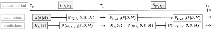
Figure 8: Sequential Bayesian updating with SPUX for datasets split across multiple time periods. Gray and white backgrounds indicate anticipated inputs and inferred outputs, respectively.

In such a case, the location of the "past" inference and the additional dataset (for period $[T_{i},T_{i+1}]$) need to be specified; unless explicitly specified otherwise, the error and units will be reused from the configuration of the specified "past" inference. If model parameters are not expected to be influenced, the model states for the next time period $[T_{i},T_{i+1}]$ can be inferred by using the PF likelihood while keeping the model parameters distribution unchanged by using the MC sampler (see the example provided in Appendix C (10) and examples/randomwalk-assimilate). Alternatively, if not only the model state but also the model parameters need to be updated when processing the next time period $[T_{i},T_{i+1}]$, a full sequential Bayesian update can be configured analogously to the example provided in subsubsection 4.3.2, but with the pastdir specified instead of the prior and initial. For an example, please refer to examples/randomwalk-update.

5 SPUX framework usage and customization

This section starts with an overview of the available framework setup options in subsection 5.1 including an overview of "sandboxing" strategies on subsection 5.2, and continues by describing key SPUX customization guidelines for the most common necessities. Those are: how to couple an application with the framework by defining a new model (subsection 5.3), including potential options to include stochastic processes for model input/parameters (subsection 5.4); how to handle model state serialization (subsection 5.5); how to specify a prior distribution for all (model and observational error) parameters (subsection 5.6); how to define an error for the available dataset(s) (subsection 5.7). In addition, subsection 5.8 describes how optional "auxiliary" output and datasets, that are not in a form of a pandas.DataFrame, can be incorporated into the model, error, and distribution classes. Multiple independent datasets can be combined using the Replicates aggregator, introduced in subsection 5.9. Instructions on possible built-in parallelization techniques for Python applications or, alternatively, on executing existing parallel user applications within the SPUX model environment are presented in subsection 5.10. Finally, subsection 5.11 provides some guidelines on advanced customization options such as writing a custom SPUX component (e.g. sampler, aggregator, likelihood, distance, etc.), with an example of SABC sampler described in subsection 5.12. SPUX documentation might incorporate improvements made after the publication of this manuscript.

5.1 Options for framework setup, component configuration and report

Multiple (non-mandatory) options to configure components, framework’s "global" setup, and the report can be specified directly in UI configuration file spux.cfg as indicated in 1 and 2. In the following, we describe the corresponding API methods and list examples of such options.

In particular, an optional configure(...) method is available for each component, implementing functionalities usually shared by all the components of a given component type. The following table provides a brief overview of all available configure-options (excluding options already introduced in the preceeding sections) for model, likelihood/distance, and sampler component types:

templatedir	None	directory with intial sandbox contents for the model
statefiles	None	sandbox files relevant to the model state (see subsubsection 5.5.1)
ignore	None	list of non-serializable model attribute names (see subsubsection 5.3.3)
timeset	4	integer: points in-between dataset snapshots; iterable: predictions times
auxset	None	auxiliary observational datasets (see subsection 5.8)
lock	None	batch index to lock sampler’s feedback to likelihood or distance

An iterable (e.g. list or array) of times $t_{0},\dots,t_{\bar{N}}$ can be used for timeset to select corresponding model outputs $y_{t_{n}}$ for later post-processing, providing additional intermediate time points (among dataset snapshots) for a larger temporal resolution (i.e. with $\bar{N}>N$).

The framework itself can be customized by the optional spux.configure(...) (see 3) and the mandatory spux.setup(...) (see 4) methods. The following basic arguments (with default values and descriptions) are available:

seed	0	integer seed (for hierarchical seeding of RNG libraries)
verbosity	2	hierarchical verbosity level (integer) for SPUX components
informative	["performance"]	to save: "performance" "timestamps" "infos" "rejections"
sandboxdir	"sandbox"	directory for the "root" sandbox (see subsection 5.2)
trace	"none"	sandboxes to keep (if used): "none" "best" "posterior" "all"
outputdir	"output"	directory for SPUX output files (see Appendix A)
history	"none"	store "statefiles"/"auxiliary": "none" "best" "posterior" "all"
states	False	store final model states for forecasting or sequential updating
checkpoint	600	minimal time period (in seconds) between checkpoints

Note, that including more keywords in informative will consequently also increase expected inference runtime, required operational memory, and the total size of written output files (see Appendix A). To keep different "statefiles" copies and archived auxiliary model predictions, a dictionary with respective "statefiles" and "auxiliary" entries can be specified for history. Refer to SPUX documentation for the advanced options (redirect, cache, setupdir) and for the additional options of functions within the test.py, synthesize.py, report.py, and best.py scripts.

5.2 Sandbox - filesystems and post-execution accessiblity

As indicated in subsection 5.1, the "root" sandbox directory sandboxdir contains nested sandboxes for each (if used) batch, chain, replicate, and model (particle or trajectory). By default, the "root" sandboxdir is placed in (node-local) fast virtual node-local RAM-based Linux filesystem called tmpfs (by default mounted at /dev/shm) to avoid network and I/O overheads. If the amount of system memory is a limiting factor, alternative (node-local) filesystems can be used to avoid network (but not I/O) overhead. For inference runs on high performance computing clusters, if neither option is possible, (shared) "scratch" file system can be used instead (with associated network and I/O overheads). If sandboxes located on node-local (not shared) filesystems are inaccessible and the functionality of the history option is not sufficient, the best (or any other) model trajectory can be re-executed (even after inference) within a specified accessible trajectorydir for model’s sandbox (see subsection 4.6).

5.3 Adding a model

In the most common use case scenario of SPUX, a user will wrap an existing application as the SPUX model either by configuring an existing SPUX model or by implementing a new SPUX model as Python class. To avoid confusion, we will refer to a user’s existing application (in any programming language) as the "application", and to the (built-in or custom) Python class coupling such application to the SPUX framework as the "model". In this section we review available model testing routines and discuss two scenarios in detail: using the built-in External model to manage the (appropriately modified) application and writing a new SPUX model class to explicitly wrap an (unmodified) application. In both cases, the incremental model execution must be possible, i.e. a corresponding output is required for each specified time from an increasing list of times.

5.3.1 Model testing and dataset synthesis

Automatically generated test.py (and synthesize.py) scripts (using the cleaned up SPUX UI spux.cfg file to only define the model component and its options) could be used to continuously test the development of a new model class. In spux.cfg, model parameters can be specified as the parametersfile option, defining the path to a text file containing rows with parameter names and values (separated by some white space), and an array of times (e.g. using utils.period(...)) for model evaluation can be specified as the snapshots option. The optional synthesize.py script uses the specified (or drawn from the prior) exact model parameters to generate exact model outputs and selected observations (with error, if specified) at the specified snapshots, including the corresponding exact.py and dataset.py scripts to load them (for instance, to generate the configuration section of the SPUX report). Such synthetically generated datasets provide an invaluable resource for making sure the correctness of your implementation, especially because the posteriors for model parameters (and outputs) obtained from the Bayesian inference can be compared to their exact values.

5.3.2 Using External model for user’s application

The External SPUX model relies on an application execution command, with which users are already familiar from using the console (shell), making this a good starting option for the first coupling of the application to the SPUX framework. In particular, the application execution command can be used to configure SPUX with an External model, as indicated by examples in 7 and 8.

Listing 7: External model example in spux.cfg.

⬇

model External

model.command r"./myapp <TIME>"

Listing 8: External model example in infer.py.

⬇

command = r"./myapp <TIME>"

model = External (command)

The External model automatically isolates the application to a unique sandbox directory, where the corresponding initial model state is written to initial.txt file if the initial model state is specified. Subsequently, the command can be executed to evolve the current model state $m_{t_{n-1}}$ to the next $m_{t_{n}}$ by reading the automatically generated input files (parameters.txt for $\theta$, time.txt for $t_{n}$ and seed.txt for the seed), and writing output.txt (see subsubsection 5.3.8 for details). Optionally, the contents of the corresponding files can be also passed to the application as runtime arguments using <PARAMETERS>, <TIME> or <SEED> keywords (for substitution) within the application command. An alternative "direct" mode of the External model is available (see later sections for reasoning) by setting model attribute direct to True. In this mode, instead of executing the command sequentially for each required time $t_{n}$, the command is executed only once to evolve model from the initial state $m_{t_{0}}$ to the final state $m_{T}$ by reading automatically generated input files times.txt and seeds.txt (or using corresponding <TIMES> and <SEEDS> keywords), and writing outputs.txt.

5.3.3 Implementing a new SPUX model class - execution control

The functionality of the simple External model might be insufficient; for instance, it might be inadequate (binary executable), inconvenient (requires changes in application interface) or inefficient (requires storing model state inbetween run(...) calls) to rely only on the application modifications.

A new SPUX model class can be written instead, allowing unrestricted capabilities for interfacing the application to the SPUX model, possibly even without any modifications to the application itself. Such model class can be specified as the "model" component within respective SPUX configuration files in 1 and 3. New model classes need to be derived from the base Model class defined in the spux.components.models.model module. The model execution flow scheme is provided in Figure 9, where arguments and built-in internal variables (introduced in subsubsection 5.3.4) are explicitly indicated for each model method.

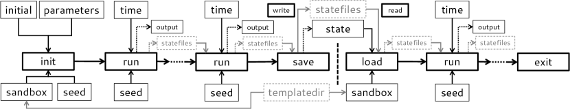
Figure 9: Execution flow scheme for the SPUX model, controlling the user’s application. The middle row indicates order of model methods calls (with multiple run and save/load calls). The top row indicates the arguments that are provided to these model methods, and the bottom row indicates before which methods the built-in variables sandbox and seed are updated.

A new SPUX model class needs to have an appropriately implemented run(...) method:

run(self,time)

run model from current time ($t_{n-1}$) until time $t_{n}$, return model output $y_{t_{n}}$

In the method declaration above, self is a handle to the model class instance, time corresponds to times in snapshots, timeset, dataset or auxset, and the model output (see subsubsection 5.3.8) consists of a mandatory array of labelled values (and, if needed, an optional "auxiliary" object). If run(...) fails (invalid parameters, invalid trajectory evolution, etc.), nothing (None) can be returned instead of raising an error, if the user would like the inference to continue. Optionally, model initialization and finalization methods can be implemented:

init(self,initial,parameters)	initialize model with initial $m_{t_{0}}$ and parameters $\theta$
exit(self)	finalize (cleanup) model after the last run(...) call

In some cases, performing the model evaluation $m\sim M(\theta)$ for all timesteps in a single function call (analogously to direct mode of the External model) instead of making incremental steps $m_{t_{n}}\sim\mathbb{P}_{n}(\cdot|m_{t_{n-1}},\theta,M)$ for each time $t_{n}$ might be an easier way to wrap the user application and/or a faster way to execute the model in cases where the incremental model execution is not required (currently it is required only by the PF likelihood). This can be achieved by implementing a custom __call__(...) method, returning model output for all times at once as a dataframe:

__call__(self,parameters,times)

given parameters and times, return model output $y$

The built-in implementation of __call__(...) relies on using init/run/exit methods and returns model outputs dataframe as well associated info and (optional) timings dictionaries (see Appendix A). Additionally, self.diagnostics attribute might be set (at runtime, by other components) to a function returning a dictionary of model output ($y_{t_{n}}$ at time $t_{n}$) diagnostics (e.g. ${\mathcal{O}}(y_{t_{n}}|\theta)$):

diagnostics(time,prediction,parameters,rng)

return diagnostics of prediction $y_{t_{n}}$

The info in __call__(...) then needs to be updated with returned diagnostics (if not None).

The implementation of model methods could rely on direct imports of modules corresponding to existing applications written in Python, could rely on customized versions of the corresponding methods found in External or Randomwalk (or in the other models from the built-in examples), or could be a combination thereof. Three choices are available to control the application execution:

basic	execute application command in a shell (an extension of the External model)
advanced	call application methods from Python using "drivers" (an efficient SPUX’onic way)
custom	implement any custom interface between the model and the application

The "basic" execution control allows extending the capabilities of the External model (see 11 in Appendix D), for instance, by storing model inputs in a different format, reading model output from a custom output file, supporting parallel applications (see subsubsection 6.1.3), implementing a custom init(...) method to account for the specified initial model state.

The "advanced" and "custom" execution control allows the control of multiple execution stages in the associated application directly from within the Python model methods, avoiding the unnecessary overhead of application initialization and finalization in-between consecutive calls of the model’s run(...) method. The computational efficiency gains are particularly large for a long time series datasets, where run(...) needs to be called multiple times, and for models with small stochastic volatility (including deterministic models), where model states filtering is infrequent (or absent) inbetween consecutive run(...) calls. In order to directly call routines within the user’s non-Python application, appropriate application-to-Python bindings can be used, with built-in examples including:

R	Python module "rpy2"	examples/runoff
Fortran	Python modules "f2py" or "ctypes" (C-ISO DLL)	examples/superflex
C/C++	Swig (swig.org) code wrapper	examples/hydro
Java	Python module "JPype1"	examples/IBM_2species

In addition to these examples, the most common practices of using the functionality of such Python bindings for SPUX are combined into so-called "drivers" under spux/drivers directory. Note, that loaded bindings or driver instances are usually non-serializable (see subsection 5.5), and hence their names as model attributes (under self) need to be included in ignore, see subsection 5.1. Next, we briefly describe built-in framework functionalities that can be used in such a new model class.

5.3.4 Model scope attributes

Any model class instance has the following relevant internal attributes accessible in all methods:

self.sandbox()	path to an isolated sandbox directory (supports file name argument)
self.parameters	model parameters $\theta$ (available if init(...) is not specified)
self.seed()	list of integer seeds for each SPUX component (and iteration)
self.seed.one()	one integer seed, reduced from an array of hierarchical integer seeds
self.rng	numpy.random.RandomState as random_state for scipy.stats
self.verbosity	integer indicating verbosity level, e.g. for custom print(...) usage
self.print(string)	print string to standard output, taking into account the verbosity
self.replace(string)	substitute <PARAMETERS>, <SEED> and <TIME> keywords in string
self.shell(command)	execute the specified command using shell in the sandbox directory

The sandboxing and seeding systems are described in more detail in the following sections. Summary implementations of methods for an external application model (External) and a Python (Randomwalk) model are provided in Appendix D, 11 and 12, respectively. For an alternative to self.shell(command) for parallel applications, see subsubsection 6.1.3.

5.3.5 Model sandbox

From within any method of the model, the path to the corresponding dedicated "local" sandbox can be retrieved by executing self.sandbox(), which might be different for each run(...) call (e.g. if PF likelihood is used). This is a path to a unique working directory for each model class instance, isolating multiple models executed in parallel and preventing race conditions and conflicts for their input/output files. Any file access within the model class can be conveniently performed using the file path returned by self.sandbox(filename). If a user’s model requires certain common files to be present in every "local" sandbox, a template sandbox directory templatedir can be specified in model.configure(...), see subsection 5.1 and Figure 9. The templatedir is best placed in parallel high performance "scratch" filesystems, since contents of the template sandbox are automatically copied (using efficient local caching) to each "local" sandbox.

5.3.6 Model seeding

Note, that self.seed(), self.seed.one() and self.rng can be different for the initialization call init(...) and for each run(...) call. The reseed() method in the test.py script checks if the model supports such frequent updates of the seeding and of the random number generator.

5.3.7 Initial model state (deterministic or stochastic)

Since the initial model state $M_{t_{0}}(\theta)$ can depend on the model parameters, it is expected to be specified as a function initial(parameters), the return value of which is passed to model’s init(...) call. Alternatively, initial(parameters) can return a prior SPUX distribution for the initial model state $M_{t_{0}}(\theta)$, a draw from which is passed to model’s init(...) call. In such case, the posterior distribution of the initial model state is then also inferred.

5.3.8 Model output

The run(...) method of the model needs to return labelled model output $y_{t_{n}}=h(m_{t_{n}},\theta)$ constructed by calling the built-in self.output(values,names,time) method. For the sake of simplicity and to keep the amount of data manageable, only a list or an array of plain datatypes (e.g. floats, integers, strings, etc.) is allowed to be specified in the argument values, with corresponding names in a list (or an array) of strings specified in the argument names. Alternatively, values can be a pandas.DataFrame with labels as index and values as the first column. For inference, all dataset (columns) labels must be present among the model output labels. For later reporting, the (extended) model ouput can contain additional labelled quantities of interest from the full model state $m_{t_{n}}$. Optional __call__(...) method of the model needs to return three objects: a dataframe for predictions $y$, an info dictionary with supporting information (including diagnostics, if requested), and timing information (or None, if not available). The predictions dataframe rows need to be indexed by times and columns labeled by names - for examples, see Model and External model classes. For the (extended) model output of a stochastic model, it could consist of multiple labelled quantities to enable, for example, additional diagnostics plots to be included in the SPUX report (see subsection 4.5):

predictions2d	summary of statistical dependencies among (extended) model output $y_{t_{n}}$ pairs
prediction2d	joint posteriors for the most correlated (extended) model output $y_{t_{n}}$ pair

In some complex models (for instance, in computational fluid dynamics), even the output prediction $y_{t}$ of the full state $m_{t}$ might consist of large multi-dimensional arrays (for instance, observed surface values) instead of just a few scalar values. In order to benefit from the built-in reporting capabilities and at the same time have an efficient method for the evaluation of the error, a diverse handful of important quantities of interest can be cherry-picked for the annotation and the (remaining or entire) output prediction $y_{t}$ can be specified as "auxiliary" (see subsection 5.8).

5.4 Processes (stochastic and deterministic)

Built-in processes for use within the SPUX model classes are available in spux.library.processes. For instance, OrnsteinUhlenbeck (i.e. bounded standard Gaussian) process with a temporal correlation length $\tau$ is available, often used to facilitate inference of time-dependent input and/or parameters for deterministic models [RM09]. In such case, the model input and/or parameters are stochastically sampled from the process evaluate(time,rng) method with rng set to model’s self.rng.

5.5 Model state serialization

The "PF" likelihood estimator for stochastic models requires the user’s model (and the underlying application) to have the capability of cloning its state $m_{s}$ at any given time "snapshot" $s$ available in the specified dataset. Additionally, the posterior forecast and sequential Bayesian updating described in subsection 2.4 and subsection 4.7 also rely on loading the final model state saved during the preceding inference run. Such capabilities of the model are also tested by the automatically generated test.py script mentioned earlier. In "clone" test, the script runs the specified model up to the specified clone time and makes a clone of the original model by saving its state. Then, a second model is created by loading the saved state of the original model and both models are run using the same seed up to the specified compare time. The outputs of both models must be identical (up to numerical roundoff errors). The "move" test checks if the model outputs are consistent in case its sandbox is moved in-between consecutive model runs. Note, that a freshly cloned model, resulting from the execution of the load method as depicted in Figure 9, does not execute the init(...) method; in particular, any required corresponding application initialization procedures need to be part of the load functionality. Furthermore, application bindings or driver instances (see subsubsection 5.3.3) are usually non-serializable and hence their names (if assigned as models attributes) need to be specified in ignore (see subsection 5.1).

In SPUX cloning is based on the concept of the model "state" serialization to a binary stream (array). There are two potential sources for application’s state information: the model class instance and, if sandboxing is used, the contents of the associated sandbox directory.

5.5.1 Model state serialization using "statefiles"

If sandboxing is used and some files in sandboxes are relevant to the model state (often corresponding to the "restart" or "pickup" files of the underlying application), then the list of all such "statefiles" (wildcards such as "*" and directories are allowed) must to be specified in model.configure(...), see subsection 5.1 and Figure 9. Such "statefiles" might be dynamically generated during the init(...) and run(...) methods of the model, and hence are not necessarily already present in the optional templatedir. If the model state is completely determined by such sandbox "statefiles" (i.e. those files are all that is required for a successful call of the run(...) method, in addition to templatedir contents), then the built-in model state serialization functionality is already sufficient, independently of the application’s programming language (including the External model from subsubsection 5.3.2). However, writing relatively large "statefiles" (in every init(...) and run(...)) as a strategy for model serialization might be inefficient due to the resulting I/O and application initialization overheads if the model state is needed only very infrequently (or if PF is not used - for instance, during forecast runs). To avoid such overhead, instead of writing and reading "statefiles" in init(...) and run(...) methods, explicit model methods for "statefiles" writing and reading can be implemented by the user:

write(self)	write "statefiles" representing model state $m_{t}$ to the model sandbox directory
read(self)	set model state $m_{t}$ by reading "statefiles" from the model sandbox directory

Note, that model sandbox is designed to contain only the "statefiles" corresponding to the current model time $t_{n}$. Any "statefiles" of the preceeding times (no longer required by run(...) method) should be removed from the model sandbox. If "statefiles" are actually required for all times (e.g. in post-processing), the history option needs to be set (see subsection 5.1) to enable automatic (within self.output(...)) "statefiles" copies to the output directory (see Appendix A).

5.5.2 Model state serialization from model class instance

If, in addition to (or instead of) the sandbox "statefiles", the model state depends on the information in the model class instance (or in the memory of the driven application), then the model serialization requirements depend on the application’s programming language. In particular, for (pickle’able) applications written in pure Python or R (using r2py bindings), the built-in model state serialization functionality is already sufficient. For applications written in other programming languages, custom methods need to be implemented to serialize the model into its binary representation (state) and to de-serialize such state into the model again (including write() and read() for "statefiles", if used):

save(self)	return a bytearray (binary array) as the current model state $m_{t}$
load(self,state)	load the specified model state $m_{t}$ represented in the bytearray

For some of the most common programming languages, built-in driver modules described in subsubsection 5.3.3 can be used to implement the above model state saving and loading.

5.6 Adding a distribution

SPUX requires all joint statistical distributions, such as model parameters prior $\pi(\cdot|M)$, error ${\mathcal{O}}(\cdot|M(\theta),\theta)$, or model initial state prior $M_{t_{0}}(\theta)$ to be defined as a SPUX Distribution. The mandatory functionality of a Distribution $X$ includes providing methods

(log)pdf(values)

evaluate the joint (log) probability density $\mathbb{P}(x)$ of values vector $x\sim X$

If the provided values are invalid, 0 and $-\infty$ should be returned, respectively. Optional capabilities, such as marginal probability density and quantile-quantile plots or initial sampler parameters drawn from $\pi(\theta,M)$, require implementation of additional Distribution methods:

(log)mpdf(label,value)	evaluate marginal (log) probability density of specific $x$[label]
intervals(alpha)	support intervals (mass alpha) of marginal probability densities
draw(rng)	draw random values vector $x\sim X$ using the provided rng

Each element of the vector $x\sim X$ has an associated label, i.e., a string, with supported LaTeX syntax (for tables and figures), such as, for example, r’$\mu$’, and an associated type (by default, random variables in Distribution are of type float). A dictionary of explicit types for each random variable label (for instance, loaded from a text file with rows of "name type" using loader.read_types(...) from spux.utils.io) can be specified in configure(types=...) of any distribution derived from the base Distribution class. Highly complex distributions represented by hierarchical Bayesian networks, where each random variable can have conditional dependencies on other variables via a directed acyclic graph, can be also constructed as a SPUX Distribution by relying on already existing respective packages, such as PyMC3 [SWF16]. In the remaining of this section we describe how to construct a Tensor distribution from univariate distributions of probabilistic libraries (such as scipy.stats) and outline available built-in transformation methods for further customization.

5.6.1 Tensor distribution

Already introduced in the Randomwalk model example in subsubsection 4.3.1, a Tensor distribution class from spux.library.distributions.tensor module provides the easiest and by far the most common way to specify a joint distribution of statistically independent univariate random variables. Only a label-indexed dictionary of required univariate distributions, for example, constructed from univariate distributions of the scipy.stats module, is needed to construct a Tensor distribution.

5.6.2 Distribution transformations

In some application scenarios, either truncated distributions might be needed (for instance, for non-negative variables), or some observations (the outputs and/or the dataset) need to be transformed before the density of the distribution from the error can be evaluated (for instance, in heteroscedastic errors). For such purposes, the built-in transformation classes for univariate distributions are available at spux.library.distributions.utils, with example usage in examples/hydro/error.py.

Truncate	truncate tail(s) of a probability density function at the specified location(s)
Concentrate	concentrate tail(s) of probability density function to an atomic part
Transform	transform any continuous distribution by an invertible function

5.7 Adding an observational error model

In SPUX, an error is defined using a function (or a callable object) which takes model output prediction $y$ and parameters $\theta$ as arguments and returns a corresponding SPUX distribution (see subsection 5.6) $D\sim{\mathcal{O}}(\cdot|y,\theta)$. Heteroscedastic errors can often be easily implemented using the distribution transformation described in subsubsection 5.6.2. The SPUX framework aims at removing systematic bias in the error by considering stochastic models instead of deterministic couterparts, and hence by default temporally independent errors are assumed, covering most of the realistic use cases. If required, temporally correlated errors can be setup by including past model outputs in output and adding lagged dataframe columns in the dataset(s), see examples/superflex.

5.8 Adding auxiliary model outputs and observational datasets

Arbitrary (pandas.DataFrame-incompatible) model outputs and datasets, such as multi-dimensional arrays or unstructured relational sets, can be also used in SPUX model, error, and distribution classes. In particular, an arbitrary "auxiliary" object can be passed in run(...) as part of the model output using output(...,auxiliary=...). Correspondingly, the prediction.auxiliary attribute will be available, for instance, in the observational error model. There, the SPUX distribution for "standard" observations can be merged with a SPUX distribution (defined using prediction.auxiliary) for "auxiliary" observations using the built-in Merge distribution from spux.distributions.merge module. An auxset dictionary with "snapshots" as time points and a "loader" as function mapping a specified snapshot to the corresponding dataset object (usually stored on a high-performance filesystem, see subsubsection 4.4.2) needs to be specified, see subsection 5.1. Note, that "auxiliary" model outputs are not returned by the model __call__(...) method; if required internally, use the model diagnostics attribute functionality instead. If history option is set (see subsection 5.1), "auxiliary" model outputs are serialized and packed into archives in output directory (see Appendix A).

5.9 Aggregating multiple datasets

In some applications (for instance, examples/hydro), multiple observational datasets are available for aggregation into the inference. Each dataset corresponds to the same model parameters $\theta$, but is a result of stochastic model evaluation with different initial model states and/or different (mutually independent) stochastic trajectories. The Replicates aggregator can be used to aggregate datasets by packing the corresponding datasets in a dictionary indexed by dataset names. The aggregator can optionally configure initial model states from an analogously indexed dictionary of corresponding initial functions, errors from a dictionary of corresponding error functions, and "auxsets" from a dictionary of corresponding auxset dictionaries.

5.10 Parallel models and parallel user applications

The example Randomwalk model introduced in section 3 does not support parallelization, and hence no executor was attached to it. However, an external user application might be very computationally expensive and might be parallel (as a stand-alone executable or as a library) or might be splittable into multiple independent tasks. In this section we introduce built-in executors for already parallel user applications and review different ways to support direct model parallelization in SPUX. The supplementary testing and synthesis scripts mentioned earlier, can also be launched for parallel models (i.e., with multiple workers attached), as described in subsubsection 4.4.2.

Since the application processes might be running on a different compute node, in local filesystems the sandbox directory can only be used for operations inside the SPUX model (not the coupled parallel user application). If the sandbox directory is explicitly required inside parallel user application, then the sandbox must be located on a shared filesystem, as described in subsection 5.2.

For applications parallelized using threads for shared memory architectures, such as multi-core CPUs or GPUs, it is sufficient (for any execution method from subsubsection 5.3.3) to properly allocate enough computational resources and properly bind SPUX MPI workers (ranks), such that each application has a dedicated part of a multi-core CPU or a GPU. If the (not yet parallelized) algorithms within model’s init/run/__call__ methods can be split into independent tasks, consider distribution across parallel workers of an attached "Pool" or "Ensemble" SPUX executor, see section 6.

In the next sections we outline available SPUX functionalities for applications parallelized using MPI (distributed memory parallelism), where the built-in parallel model executor is attached to the user’s model with the specified number of workers. In particular, "basic" mode replacing the built-in self.shell(...) is described in subsubsection 5.10.1. Despite its generality and simplicity, the "basic" model executor mode could be inefficient due to multiple application execution calls. Alternative model executor modes ("advanced" and "custom") are introduced in subsubsection 5.10.2 and subsubsection 5.10.3 (with supplementary subsubsection 5.10.4), requiring only a single application launch (e.g. loading a library or executing a process) and relying on application execution control within init/run/__call__ methods. Such model executor modes allow one to avoid unnecessary filesystem related operations and excessively large number of state saving/loading or "statefiles" writing/reading by implementing custom write/read or save/load methods (see subsection 5.5). A guideline scheme for selecting the appropriate executor mode for the model based on the available parallel features of the user’s application and of the MPI library is available in Figure 10.

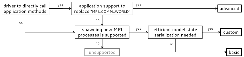
Figure 10: A guideline scheme to select the appropriate parallel model executor mode based on the characteristics of the application and of the MPI library.

5.10.1 Parallel model executor for parallel user applications - "basic" mode (execute)

As an extension of the "basic" execution mode in subsubsection 5.3.3, the "basic" parallel model executor replaces the built-in self.shell(...) in init/run/__call__ methods with

self.executor.execute (r’application’, args = [’arg1’, ’arg2’])

This way, each application is executed (spawned) in parallel (in the respective sandbox directory), analogously to the manual launch using MPI. For correct model serialization, model (and application) state within init(...) and run(...) methods can be directly stored as model instance (self) attributes and/or as files (e.g. "statefiles") in its sandbox (without explicit write/read methods).

5.10.2 Parallel model executor for parallel user applications - "advanced" mode (instruct)

As an extension of the "advanced" model execution method from subsubsection 5.3.3, the "advanced" parallel model executor mode relies on direct (but minimally intrusive) application control. In particular, on each parallel application worker in the peers intra-communicator, a function to establish and return (e.g. using drivers, see subsubsection 5.3.3 and Appendix E) an interface to the application

interface = method (manager, peers)

can be specified for the built-in parallel model executor establish(...) method:

self.executor.establish (method)

User-defined instruction functions are required to call application method(s) on each parallel worker (with the MPI intra-communicator peers instead of MPI_COMM_WORLD) using the binded interface:

result = instruction (interface, peers)

SPUX model acts as a "manager" to control application: specify parameters, retrieve output, and save/load model state or write/read "statefiles". To achieve this, custom instruction functions (see also Appendix E for a practical example) can be defined (even at runtime within model methods, if specified model parameters, time, seed, etc. need to be taken into account). An instruction function can be dispatched from (any method of) the SPUX model (as the "manager") to all parallel application processes (as "workers") for execution and retrieval of returned instruction results by calling:

results = self.executor.instruct (instruction)

Application interface can be terminated by self.executor.demolish() in the model exit().

5.10.3 Parallel model executor for parallel user applications - "custom" mode (connect)

As an extension of the "custom" model execution mode introduced in subsubsection 5.3.3, a "custom" parallel model executor mode can be used to launch (spawn) the application, e.g. in init(...), with

self.executor.launch (r’application’, args = [’arg1’, ’arg2’, ’<PORT>’])

where strings <PORT> among the list of arguments will be replaced by the actual port, described in later subsubsection 5.10.4. Afterwards, the manager-side (i.e. SPUX model) MPI inter-communicator to the parallel workers (i.e. user application) can be obtained and released by, respectively:

workers = self.executor.connect() and self.executor.disconnect(workers)

executor method calls in any model method, as many times as required. Note, that the MPI communicators are not serializable and hence must be added to the ignore list (see subsection 5.1) if stored as model (i.e. self) attributes. The manager-side MPI inter-communicator to workers can be used for simulation control, parameters specification, output retrieval, saving/loading of the model state or writing/reading of "statefiles", and for termination of application execution in model exit().

5.10.4 Application-side communicators for parallel user application in "custom" mode

In the "custom" model executor mode, in addition to a standard intra-communicator among other application workers (usually MPI_COMM_WORLD, as in a manual MPI run), each parallel worker (of the user’s application) also retrieves a corresponding worker-side inter-communicator with the "manager" (the model) by calling MPI_Comm_Connect(port,...). The port can be passed as the command line argument (or, alternatively, as a file in the model sandbox) to the application executable. The worker-side MPI inter-communicator to "manager" can be used to manage the execution flow within the user’s application according to the requests from the manager side (parameters acquisition, output reporting, saving/loading model state and writing/reading "statefiles", etc.).

5.11 Adding an arbitrary SPUX component

In this section we briefly overview guidelines for adding new SPUX component algorithms (e.g. for sampler, aggregator, likelihood or distance component types), or even new SPUX component types.

A new SPUX component algorithm class inherits the corresponding component type class, and can potentially re-define mandatory require dictionary and/or optional configure method (as in configure.py), see Appendix F, 15. The require dictionary contains "executor" with an attachable executor type name (from subsection 6.1 with default being "Pool") and (optionally) "tasks" with a list of assignable component type names (absent by default). Optional init and mandatory __call__ methods of the component algorithm class are responsible for the actual computations (as in infer.py) and can access self.sandbox, self.seed and self.rng instances.

A new SPUX component type class (i.e. a row in the components table, subsection 3.1) inherits the Component class, defines the mandatory component attribute (a string for type name), and can re-define the require attribute and the optional configure method, see Appendix F, 16. The Component class from the spux.components.component module implements default attributes and methods common among all SPUX component type classes, such as name, require, evaluations, assign, attach, copy, setup, isolate, plant, spawn, consensus, feedback, feed, prepare.

5.12 Approximate Bayesian Computation type samplers

In ABC-type samplers (introduced in subsubsection 2.3.3), the (approximate-)likelihood based samplers are replaced by approximate samplers based on an empirical distance between the appropriate summary statistics $\mathcal{S}(y)$ of model output $y$ and $\mathcal{S}(D)$ of the observational dataset $D$, as depicted in the adapted SPUX framework scheme in Figure 11. If, in addition, the (optional) observation error model is available, then it will be incorporated into the model output before the distance evaluations. Alternatively, the user’s SPUX model might already contain all required uncertainties arising from both the generative (deterministic or stochastic) model and the stochastic error, in which case the observational errors are also incorporated for the distance evaluations. However, the explicitly defined error model (i.e., not part of the generative model) allows for future forecast of true model output, whereas hiding the error within the generative model only allows for future forecast of observed (i.e., including observational noise) model output.

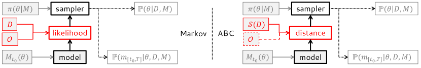
Figure 11: Differences in the components configuration for the SPUX framework using ABC-type sampler (right part). The components that are different from the Markov-type samplers (left part, refer to Figure 5 for a detailed description) are highlighted in red.

For the ABC-type samplers, the number of required posterior samples can be set by specifying the batchsize for the sampler constructor, and the number of iterations for convergence can be set by specifying the batches (instead of the samples for the Markov-type samplers) for the call sampler(...). For an example using the SABC sampler, please refer to examples/randomwalk-sabc.

6 SPUX framework parallelization

In this section we describe three built-in executor types and their load balancing techniques. For the design and implementation of the hierarchical parallelization sub-system supporting multiple nested executors for simultanous parallelization of multiple nested SPUX components, see Appendix H.

6.1 SPUX executors - types

Any set of independent tasks within any of the SPUX components can be executed in parallel using built-in SPUX executors. The parallel design of SPUX is centered on three main types of executors, each supporting different functionality and (usually) meant to be used in different SPUX components:

pool	dynamically executes a set of independent tasks; task "states" are discarded
ensemble	adaptively executes a set of independent ensemble tasks (maintaining task "states")
model	dynamically executes a user’s application (discarding or maintaining its "state")

Executors can be attached to SPUX components without any restrictions on the executor type, however, the list of available executor capabilities (methods) is checked at the attach(...) method of the corresponding SPUX component. As described in the tutorial, the default executors of each type are the serial executors with rather straight-forward implementations, namely SerialPool, SerialEnsemble, SerialModel. Currently, parallel executors of each type are implemented in SPUX using the Message Passing Interface (MPI) library [Mes15] via the object-oriented Python MPI bindings package mpi4py [DPKC11]. MPI dynamic process management for parallel workers is employed for deploying nested parallelization. Pickle-based communication of arbitrary serializable Python objects is used for execution workflow management across managers and workers, as the memory and processing time overheads are negligible. Additionally, for multiple subsequent executor calls (e.g. for iterative sampling within sampler), executor task caching allows to perform task serialization and communication only once. Finally, memory-efficient raw binary arrays (bytearray) are used for efficient communication of model states.

6.1.1 SPUX "pool" executors

A "pool" type executor can be used by calling its map(functions,parameters) method, where either argument (or both) can also be iterable (for instance, a list) over corresponding parallel tasks. For lower communication overhead, consider providing lists of sandboxes and/or seeds as arguments in map(...) instead of using lists of functions. An optional list of arguments can be specified in map(...) as args and will be passed to the execution of the function(s) by function(...,*args).

6.1.2 SPUX "ensemble" executors

An "ensemble" type executor does not accept tasks directly, but requires an instance derived from the Ensemble base class defined in the spux.library.ensembles.ensemble module. Currently the only implemented ensemble class is for a Particles ensemble of SPUX models (particles to be used in the PF likelihood). For example, the "ensemble" executor, attached to an instance of the PF likelihood, manages the parallel initialization, method execution and resampling of (indexed) ensemble tasks. In particular, in-between the ensemble executor connect(ensemble,indices) and disconnect() methods, call(method,args) and/or resample(indices) methods can be called multiple times, each time executing the specified ensemble method and/or performing ensemble resampling, respectively. In the resample method, ensemble tasks can be cloned (duplicate indices) and deleted (missing indices), including the load re-balancing across the resampled sub-ensembles. A detailed description of the parallel resamplig procedure is available in the earlier manuscript [ŠK17].

6.1.3 SPUX "model" executors

A "model" type executor is needed to execute a parallel user application. As described in subsection 5.10, three parallel model executor modes to manage parallel application workers are supported:

basic	execute(command) by spawning a new process (analogously to mpiexec)
advanced	instruct(...) to call instruction(...) with MPI intra-communicator peers
custom	launch(application) and connect()/disconnect() MPI inter-communicators

Options, such as args list of runtime arguments, can be specified in execute(...) and launch(...) methods. For serial executors (workers set to None or 0), both methods fall back to shell(...).

6.2 SPUX executors - load balancing

In all parallel executors, a collection of multiple tasks must be carefully dispatched to (or re-distributed among) parallel workers to ensure the minimal needed wall-clock runtime to execute all tasks. In this section we describe such load balancing algorithms for the pool and ensemble type executors. For "model" type executors, the load balancing is federated to the user’s application itself.

6.2.1 Load balancing for pool-type executors

All tasks requested in the "map" method of the "pool" type executor are executed dynamically, with pending tasks being constantly dispatched to workers as they become available. For parallel runs with multiple datasets (e.g. examples/hydro example), the Replicates aggregator performs guided load balancing by evaluating the lengths of the associated datasets and sorting component evaluations, taking into account the component adaptivity as well (for instance, the replicate-dependent adaptive number of particles in the PF likelihood). Higher priorities are assigned to components with longer datasets and large number of particles (if applicable), and lower priorities are assigned to the components with shorter datasets and smaller number of particles (if applicable).

6.2.2 Load balancing for ensemble-type executors

During routing, re-sampled tasks are instructed to be moved from over-utilized workers to the neighboring under-utilized workers across their intra-communicator. Routing objects include worker-specific information regarding task identification, source (present worker address), destination (re-routed worker address), re-identification (for post-routing re-seeding), and affinity (local or remote node). An empirical greedy algorithm is employed for constructing routings based on re-sampled task counts, current task distribution across workers, and the maximal worker load. For each worker, resident re-sampled tasks are kept in place provided the worker loads do not exceed the maximal worker load. Remaining tasks are routed either to a under-utilized worker on the same compute node (determined by affinity), or, in the worst case, to the closest (w.r.t. proximity of worker ranks) under-utilized remote worker. To further reduce communication overhead, identical tasks are moved together by moving only a single particle and then replicating it on the destination worker. Such load balancing strategy, however, does not take into account possibly heterogeneous model runtimes for each task, and hence there could be potential gains from dynamic balancing frameworks using task stealing instead of an adaptive routing approach. Sandboxes, associated to the corresponding tasks, are assumed to be isolated from each other, unless local affinity (determined automatically) is set in the routing information. For local affinity, sandboxes exist on the same compute node (with access to the same filesystem), and hence a simple and efficient sandbox renaming (internally consisting of stashing and fetching) is sufficient. Such "hybrid" parallelization, inspired by existing MPI + OpenMP paradigms, harnesses the node-local connectivity to minimize the required sandbox-related communication. For remote affinity, sandboxes are "pseudo-moved" from one remote filesystem to another, by copying template sandbox on the destination, and, if sandbox "statefiles" are specified, saving the sandbox state, sending it to the destination, and loading it into the newly created sandbox. After removal of all extinct particles, at the expense of memory usage the resampling process prioritizes overlapping the communication synchronization overhead with any other pending task that does not require information exchange with other parallel ensemble workers. In particular, after all asynchronous sends and receives for task exchange according to routings are launched, all orphan particles (already sent, but not to be kept) are removed, remaining particles are stashed, ensembles are synchronzed to prevent race conditions, stashed particles are fetched using re-identification, local particles are replicated, and only in the last step received remote particles are stored and replicated, while still waiting in the background for all local particles (if any) to be sent. For a more detailed description and an illustrative scheme of such adaptive ensemble task resampling, refer to the earlier manuscript [ŠK17].

7 Future developments

In the near future, multi-level uncertainty quantification methods (e.g. ML(ET)PF, MLCV) will be investigated. These methods can greatly reduce the amount of required computational resources for Bayesian inference and forecasting by configuring applications for multiple different accuracies (e.g. resolutions). These capabilities will be offered in SPUX through the the foreseen MLCV aggregator component. Furthermore, samplers optimized for multi-modal posteriors will be investigated. Additionally, shared memory optimizations for nodel-level model state communication, dynamic balancing using task stealing in ensemble tasks resampling, and machine learning based dynamical process scheduling for pool executors are foreseen as further improvements of an already very well performing SPUX parallelization suite. Depending on the level of support for general purpose distributed tasking libraries, new parallel executors could be added.

8 Author contributions and acknowledgments

Author contributions. JŠ designed and implemented the prototype framework, plotting, automatic report generation, compiled the documentation, contributed examples for built-in and "hydro" models, and led the preparation of this manuscript. JŠ and MB co-designed and implemented the parallelization specification, all main SPUX components, and SPUX interfaces (UI and API). MB also designed and implemented the legacy MPI connector, distribution variable types, and contributed examples for "superflex" and "ibm" models.

Acknowledgments. Authors would like to thank Uwe Schmitt and Mikołaj Rybiński (ETH Zurich) for support with CI/CD and unit testing on EULER and Daint clusters at the Swiss Supercomputing Center (CSCS), Artur Safin, Marco Dal Molin and Lorenz Amman (Eawag) for contributing example models, Mira Kattwinkel (U Koblenz-Landau) for helping to design the initial SPUX framework prototype, Alexander Madsen (PSI), Anthony Ebert (USI and Eawag), Simone Ulzega (ZHAW) for contributing and testing SABC sampler, Peter Reichert (Eawag), Andreas Scheidegger (Eawag), Carlo Albert (Eawag), Fabrizio Fenicia (Eawag), Vilma Šukienė for providing feedback to this manuscript and framework usage, Panagiotis Hadjidoukas (IBM Research Zurich) for advice regarding task-based parallelism design, and Siddhartha Mishra (ETH Zurich) for access to EULER cluster.

Funding. We also acknowledge the Eawag Directorate Discretionary Funding for granting financial resources and Swiss Supercomputing Center (CSCS) for granting computational resources in the development project d97.

Appendix A SPUX setup and output

The setup directory contains generated raw (binary, text, and LaTeX) information regarding SPUX framework configuration and setup, corresponding to configure.py and infer.py, respectively. The output directory is generated incrementally using checkpointing and contains multiple subdirectories:

samples	samples of posterior parameters, outputs, supporting "infos", timings
best	the "best" trajectory (parameters and output); also see LABEL:R-t:randomwalk_best-specification
diagnostics	diagnostics information (e.g. metrics)
specifications	structure specifications of the outputs/infos files and the "best" trajectory
pickup	framework (e.g. sampler) pickup information (for --continue)
states	final states samples of posterior model trajectories
statefiles	(only if used) copies of "statefiles" for all times
auxiliary	(only if used) auxiliary model outputs

Contents of the samples subdirectory can be loaded and used for any custom post-processing:

parameters-*.csv	a CSV file containing posterior samples of model parameters
predictions-*.dat	a binary file containing (posterior) of model output samples
infos-*.dat	a binary file containing supporting information (e.g. acceptance rates)
timings-*.dat	a binary file containing framework timings (runtimes and timestamps)

Refer to report.py for an example of loading all samples files into dataframes (for CSV) and lists of dictionaries using loader.reconstruct(...) from spux.utils.io. The corresponding specifications tables are also listed in the LABEL:R-s:report-specifications of the SPUX report as LABEL:R-t:randomwalk_predictions-specification, LABEL:R-t:randomwalk_infos-specification, and LABEL:R-t:randomwalk_timings-specification. In particular, each model predictions (output) sample is a dictionary of either dataframes (default) or Trajectories from spux.utils.trajectories module (using memory-efficient compressed data structures [JMR15], e.g. for PF).

Infos contain additional (component-specific) information for "infos" keyword requested in informative and/or for a manually specified component (such as PF likelihood or Norm distance) diagnostics list. Unless "rejections" keyword is requested in informative, model outputs and infos corresponding to the rejected samples are excluded (set to None), and the estimates of prior and likelihood/distance are overwritten by the values of the accepted samples.

To ensure consistency, we strongly advice to access any SPUX framework output (or configuration and setup options) using the SPUX status, which can be constructed using the Status class from the spux.utils.status module, as is done in report.py. Attribute status.parameters is a pandas.DataFrame loaded directly from parameters-*.csv, and additional status methods can be called with any required batch/chain/time arguments:

info(key,...)	respective key value from loaded infos-*.dat
prediction(...)	respective model prediction from loaded predictions-*.dat
timing(...)	respective timing measurement from loaded timings-*.dat
sandbox(...)	respective model sandbox path (relative to the "root" sandbox)
auxiliary(...)	respective "auxiliary" model output (see subsection 5.8)
statefiles(...)	respective paths to directories storing all "statefiles" (see subsubsection 5.5.1)

Internally, these methods use "origins" stored in sampler "info" to locate the corresponding accepted samples and functionality of the Trajectories class to follow trajectory filtering (if PF was used).

The figures directory contains all raw figure files in multiple formats (default: PDF (vector), PNG (raster)) and with the associatiated caption files *.cap containing the description of the figure contents. The contents of the setup and figures directories are used to generate the LaTeX source files in the report directory, which are compiled into the SPUX report (A4 and "slides" layouts).

Appendix B Remark on workers for parallel SPUX executors

The freedom to attach arbitrary many parallel workers for every SPUX component provides a lot of flexibility, but also leaves ample space for computationally inefficient parallel configurations. Hence, for large production runs, we strongly advice to follow these two guidelines:

• Attach most workers to the outer-most SPUX component(s) (e.g. sampler).

• Avoid few parallel workers (less than 4) - replace them with the default workers = None.

SPUX will report the percentage of the number of manager cores w.r.t. the total number of cores. Additionally, parallel performance and scaling plots could be used to investigate the model runtimes homogeneity and the synchronization overheads. For highly heterogeneous model runtimes (for instance, when model runtime strongly depends on the proposed model parameters), or for the cases where sampler often proposes parameters outside the specified prior parameters distribution, consider attaching more workers to the PF likelihood instead in order to avoid very few tasks for each parallel worker in sampler (and aggregator) SPUX components.

Appendix C Example forecast and sequential assimilation scripts

Listing 9: Example spux.cfg for forecast

⬇

model Randomwalk

model.dt 0.1

aggregator Trajectories

aggregator.trajectories 64

sampler MC

sampler.chains 64

sampler.samples 500

pastdir "../randomwalk"

timeset utils.period (25, 30)

Listing 10: Example spux.cfg for assimilation

⬇

model Randomwalk

model.dt 0.1

likelihood PF

likelihood.particles 256

sampler MC

sampler.chains 64

sampler.samples 1000

pastdir "../randomwalk"

dataset dataset-T_1-T_2.py

Appendix D Example model scripts

Listing 11: External model methods

⬇

from spux.utils.io import loader

from spux.utils.io import dumper

def run (self,time):

p = self.sandbox("parameters.txt")

t = self.sandbox("time.txt")

s = self.sandbox("seed.txt")

dumper.txt(p,self.parameters)

dumper.txt(t,self.time)

dumper.txt(s,self.seed())

cmd = self.replace(self.command)

code = self.shell(cmd)

if code is None: return None

o = self.sandbox("output.txt")

return self.output(loader.txt(o))

Listing 12: Randomwalk model methods

⬇

def init (self,initial,parameters):

self.d = parameters["drift"]

self.v = parameters["volatility"]

self.m = initial["position"]

self.time = initial["time"]

def run (self,time):

while self.time < time:

dt = min(time-self.time,self.dt)

n = self.rng.normal()

self.m += dt*self.d

self.m += sqrt(dt)*self.v*n

self.time += dt

return self.output([self.m],[’p’])

Appendix E Example parallel model executor scripts for Fortran

In 13, the application module is obtained by compiling user’s Fortran application with f2py. On parallel application workers, the returned interface is passed to instruction in 14.

Listing 13: Application interface example

⬇

def interface (manager,peers):

import application

interface = application

return interface

Listing 14: Executor instruction example

⬇

def instruction (interface,peers):

comm = peers.py2f()

result = interface.main(comm)

return result

Appendix F Example SPUX component scripts

Listing 15: Component algorithm class example

⬇

class NewAlgorithm (NewType):

def init (self,...):

...

def __call__ (self,...):

...

Listing 16: Component type class example

⬇

class NewType (Component):

component = "new_type"

requires = {"executor":"Pool"}

def configure (self,...):

...

Appendix G Adaptivity in the Particle Filter

For the SPUX framework, we are also introducing an empirical adaptivity technique to dynamically control the number of particles used for the PF likelihood. The proposed technique, as already common among complex adaptive methodologies such as [EMD17], relies on empirical metrics; in this case, on "fitscore", which describes the convergence progress of the posterior sampling, and on "accuracy", which provides an estimate for the statistical error in the estimated likelihood.

G.1 Fitscores of model parameters

A fitscore indicator is simply the likelihood normalized (purely for easier interpretation and generalization) w.r.t. the dataset length, dimensionality of the observations, and the maximum of the corresponding error distribution densities. As such, fitscore measures (analogously to likelihood) how consistent the model output is compared to the observational dataset. Recalling the notations

$${\mathcal{O}}_{n}(D|y,\theta)={\mathcal{O}}(D_{t_{n}}|y_{t_{n}},\theta),\quad{\mathcal{O}}_{n}^{p}(D|y,\theta)={\mathcal{O}}_{n}(D|y^{p},\theta),\quad{\mathcal{O}}_{n}(D|y,\theta)=\frac{1}{P}\sum_{p=1}^{P}{\mathcal{O}}_{n}^{p}(D|y,\theta),$$ (12)

we define fitscore as the average (over multiple dataset points $N$ and multiple particles $P$ of the Particle Filter) logarithm of the normalized (with respect to probability density function value of the model prediction and the dimensions $d$ of the observations) residuals (observational model error probability density of posterior model output):

$$r(\theta,D,M)=\frac{1}{N}\sum_{n=1}^{N}\frac{1}{P}\sum_{p=1}^{P}\frac{\log{\mathcal{O}}_{n}^{p}(D|y,\theta)-\log{\mathcal{O}}_{n}^{p}(y|y,\theta)}{d}.$$ (13)

The numerical value of the fitscore empirically tracks progress of the sampler convergence, with higher values indicating that the sampler is most probably out of burn-in phase.

G.2 Accuracies of likelihood estimates

The variance $\sigma^{2}(\log\hat{L})$ of the estimated marginal log-likelihood $\log\hat{L}$ was found to be an important indicator controlling the convergence of the Markov chain sampler [KR17]. It can be bounded (with equality only for statistically independent ${\mathcal{O}}_{n}$ over all $n=1,\dots,N$) by the sum of log-likelihood variances from individual snapshots (for brevity, we drop $(D|y,\theta)$ notation from ${\mathcal{O}}_{n}^{p}$ and ${\mathcal{O}}_{n}$):

$$\sigma^{2}(\log\hat{L})=\sigma^{2}\left(\log\left(\prod_{n=1}^{N}{\mathcal{O}}_{n}\right)\right)=\sigma^{2}\left(\sum_{n=1}^{N}\log{\mathcal{O}}_{n}^{p}\right)\leq\sum_{n=1}^{N}\sigma^{2}(\log{\mathcal{O}}_{n}).$$ (14)

Motivated by this upper bound, the empirical "accuracy" of the PF likelihood is defined as the average (over multiple dataset points) standard deviations for the estimated observational log-errors (treated as random statistical estimates depending on $p$):

$$\delta(\theta,D,M)=\frac{1}{N}\sum_{n=1}^{N}\sigma(\log{\mathcal{O}}_{n}).$$ (15)

The numerical value of the accuracy empirically measures the statistical accuracy of the marginal likelihood estimator computed by the Particle Filter, normalized with respect to the length $n$ of the dataset. The standard deviations $\sigma(\log{\mathcal{O}}_{n})$ for the estimated observational log-errors of the current snapshot, are dynamically (i.e., during runtime) estimated using 1st order Taylor-series approximation and the central limit theorem. In particular, the variance of the logarithm of a random variable $a$ can be approximated using Taylor series around the mean $\mu(a)$:

$$\sigma^{2}(\log a)\approx\frac{\sigma^{2}(a)}{\mu^{2}(a)},\quad\textnormal{provided}\quad\sigma^{2}(a)\ll\mu^{2}(a).$$ (16)

The summands $\sigma(\log{\mathcal{O}}_{n})$ in equation 15 can be approximated by such Taylor-series by setting $a={\mathcal{O}}_{n}$ and then applying a central limit theorem to approximate $\mu({\mathcal{O}}_{n})$ and $\sigma({\mathcal{O}}_{n})$ by $\hat{\mu}({\mathcal{O}}_{n})$ and $\hat{\sigma}({\mathcal{O}}_{n})$:

$$\mu({\mathcal{O}}_{n})=\mu({\mathcal{O}}_{n}^{p})\approx\hat{\mu}({\mathcal{O}}_{n}^{p})=\frac{1}{P}\sum_{p=1}^{P}{\mathcal{O}}_{n}^{p}={\mathcal{O}}_{n},\quad\sigma^{2}({\mathcal{O}}_{n})=\frac{\sigma^{2}({\mathcal{O}}_{n}^{p})}{P}\approx\frac{\hat{\sigma}^{2}({\mathcal{O}}_{n}^{p})}{P}.$$ (17)

In Equation 17, $\hat{\mu}({\mathcal{O}}_{n}^{p})$ and $\hat{\sigma}({\mathcal{O}}_{n}^{p})$ are the empirical estimators for the mean and the variance as computed from the available $p$ samples ${\mathcal{O}}_{n}^{1},\dots,{\mathcal{O}}_{n}^{P}$ of the random variables ${\mathcal{O}}_{n}$. Applying both approximations, the final estimate for the "accuracy" is then given by

$$\delta\approx\frac{1}{N}\sum_{n=1}^{N}\frac{\sigma({\mathcal{O}}_{n})}{\mu({\mathcal{O}}_{n})}\approx\frac{1}{N}\sum_{n=1}^{N}\frac{1}{\sqrt{P}}\frac{\hat{\sigma}({\mathcal{O}}_{n}^{p})}{{\mathcal{O}}_{n}}.$$ (18)

G.3 Adaptivity procedure and customization

Initially, all particle filters start with the minimal number of particles (default is 4 or the number of parallel workers for PF). Fitscore values above the customizable threshold (with the default value at -2) indicate that the sampler is most probably out of the initialization phase, and hence the particle filter adaptivity is activated. The number of particles is then halved or doubled in each likelihood estimation step, depending on whether the accuracy is above or below the requested accuracy envelope. Requested accuracy envelope is determined by the accuracy and margins specified within the adaptive PF likelihood. The maximum number of particles is given by particles option of PF. To guarantee the convergence of the posterior, the particle adaptivity is suspended after the user-specified "lock" sample batches.

Appendix H SPUX executors - design

The schemes outlining designs of the SPUX executor (the manager side) and the corresponding SPUX contract (the worker side) are listed in Figure 12 and Figure 13, respectively.

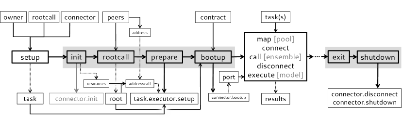
Figure 12: Execution flow scheme for the SPUX executor base class (the manager side). The thick solid arrows represent the sequence of the called methods (the gray arrow indicates a call at the top-level executor only), the thin solid arrows represent the required inputs, and the dotted arrows represent the outputs (or inputs provided to subsequently called methods). The tasks-to-results pipeline can then be executed multiple times, with the final executor exit() deallocating all computational resources.

In Figure 12, during the configuration stage when executors are attached to SPUX components, only the setup of each executor is called and only with the owner argument. Such pre-setup executors are then used to compute the total required resources in framework init(...). After the configuration stage, the init(...) of the executor attached to the main component (sampler) is called by framework init(...) and initializes the connector (i.e. allocates computational resources). The same executor init(...) method then starts a chain of recursive hierarchical initializations for all other executors. In particular, the setup(...) of the executor attached to the task of the owner of the current executor is called, where the task of the executor owner becomes the owner of the task executor, and the addresscall() of the executor is used for the rootcall of the task executor. During the bootup(...), each parallel worker is issued a contract describing required worker behavior, as explained in Figure 13.

Figure 13: Execution flow scheme for the SPUX contract (the worker side) required in SPUX executors. The boxes with dashed outline represent the communicators and the dashed arrows represent the information exchange over the network. The thick solid arrows represent the sequence of the called methods, the thin solid arrows represent the required inputs, and the dotted arrows represent the outputs (or inputs provided to subsequently called methods). The pipeline part highlighted with the gray outline can be executed multiple times.

In Figure 13, the manager and peers communicators are provided as the arguments of the contract. Initially, the port (to connect back to manager) and the executor (to be attached to incoming tasks) for each worker’s contract is received by the workers from the manager communicator. The taskroot (integer or string) is determined by the rootcall(...) of the task executor, which is set in task.executor.setup (...), see Figure 12. The taskport (integer or string) is determined by calling init(...) of the received task executor, completing this way the next recursive step of hierarchical executor initializations. The contract then waits for further instructions from the manager, for instance, to execute some tasks. The determined taskroot and taskport are unique among all other peer task executors (initialized in the contracts of parallel workers at the same hierarchical level), and hence can be used for binding any requested task to the task executor initialized specifically for this contract. The results obtained by executing the received tasks are then sent back to the manager.

References

- [ABD+09] Brian M Adams, WJ Bohnhoff, KR Dalbey, JP Eddy, MS Eldred, DM Gay, K Haskell, Patricia D Hough, and Laura P Swiler. Dakota, a multilevel parallel object-oriented framework for design optimization, parameter estimation, uncertainty quantification, and sensitivity analysis: version 5.0 user’s manual. Sandia National Laboratories, Tech. Rep. SAND2010-2183, 2009.
- [ADH10] Christophe Andrieu, Arnaud Doucet, and Roman Holenstein. Particle Markov chain Monte Carlo methods. Journal of the Royal Statistical Society: Series B (Statistical Methodology), 72(3):269–342, 6 2010.
- [AKS15] Carlo Albert, Hans R Künsch, and Andreas Scheidegger. A simulated annealing approach to approximate bayes computations. Statistics and computing, 25(6):1217–1232, 2015.
- [AUS16] Carlo Albert, Simone Ulzega, and Ruedi Stoop. Boosting bayesian parameter inference of nonlinear stochastic differential equation models by hamiltonian scale separation. Phys. Rev. E, 93:043313, Apr 2016.
- [BCJ+18] Eli Bingham, Jonathan P. Chen, Martin Jankowiak, Fritz Obermeyer, Neeraj Pradhan, Theofanis Karaletsos, Rohit Singh, Paul Szerlip, Paul Horsfall, and Noah D. Goodman. Pyro: Deep Universal Probabilistic Programming. Journal of Machine Learning Research, 2018.
- [CGH+17] Bob Carpenter, Andrew Gelman, Matthew D Hoffman, Daniel Lee, Ben Goodrich, Michael Betancourt, Marcus Brubaker, Jiqiang Guo, Peter Li, and Allen Riddell. Stan: A probabilistic programming language. Journal of statistical software, 76(1), 2017.
- [CRSF16] Fernando Chirigati, Rémi Rampin, Dennis Shasha, and Juliana Freire. Reprozip: Computational reproducibility with ease. In Proceedings of the 2016 International Conference on Management of Data, SIGMOD ’16, pages 2085–2088. ACM, 2016.
- [DJ09] A. Doucet and A.M. Johansen. A tutorial on particle filtering and smoothing: Fifteen years later. Handbook of nonlinear filtering, 12:656–704, 2009.
- [DMRT14] J Doherty, C Muffels, J Rumbaugh, and M Tonkin. Pest, model independent parameter estimation and uncertainty analysis, 2014.
- [DPKC11] Lisandro D. Dalcin, Rodrigo R. Paz, Pablo A. Kler, and Alejandro Cosimo. Parallel distributed computing using Python. Advances in Water Resources, 34(9):1124–1139, 2011.
- [DSN+14] Omer Demirel, Ihor Smal, Wiro J Niessen, Erik Meijering, and Ivo F Sbalzarini. Ppf: A parallel particle filtering library. 2014.
- [DSU+17] Ritabrata Dutta, Marcel Schoengens, Avinash Ummadisingu, Nicole Widmer, Jukka-Pekka Onnela, and Antonietta Mira. Abcpy: A high-performance computing perspective to approximate bayesian computation. arXiv preprint arXiv:1711.04694, 2017.
- [duc18] Glossary — python 3.7.1 documentation, 2018.
- [eas20] Easyabc, 2020.
- [EMD17] V. Elvira, J. Míguez, and P. M. Djurić. Adapting the number of particles in sequential monte carlo methods through an online scheme for convergence assessment. IEEE Transactions on Signal Processing, 65(7):1781–1794, 2017.
- [FMHLG13] Daniel Foreman-Mackey, David W Hogg, Dustin Lang, and Jonathan Goodman. emcee: the mcmc hammer. Publications of the Astronomical Society of the Pacific, 125(925):306, 2013.
- [GC17] A. Gregory and C. J. Cotter. A seamless multilevel ensemble transform particle filter. SIAM Journal on Scientific Computing, 39(6):A2684–A2701, 2017.
- [GCS+14] Andrew Gelman, J. Carlin, H. Stern, D. Dunson, A. Vehtari, and D Rubin. Bayesian Data Analysis, third ed. Chapman & Hall, 2014.
- [GDB+19] Carla Gomes, Thomas Dietterich, Christopher Barrett, Jon Conrad, Bistra Dilkina, Stefano Ermon, Fei Fang, Andrew Farnsworth, Alan Fern, Xiaoli Fern, Daniel Fink, Douglas Fisher, Alexander Flecker, Daniel Freund, Angela Fuller, John Gregoire, John Hopcroft, Steve Kelling, Zico Kolter, Warren Powell, Nicole Sintov, John Selker, Bart Selman, Daniel Sheldon, David Shmoys, Milind Tambe, Weng-Keen Wong, Christopher Wood, Xiaojian Wu, Yexiang Xue, Amulya Yadav, Abdul-Aziz Yakubu, and Mary Lou Zeeman. Computational sustainability: Computing for a better world and a sustainable future. Commun. ACM, 62(9):56–65, August 2019.
- [GL06] D. Gamerman and H.F. Lopes. Markov Chain Monte Carlo: Stochastic Simulation for Bayesian Inference. Taylor & Francis Inc., 2006.
- [HAPK15] Panagiotis E Hadjidoukas, Panagiotis Angelikopoulos, Costas Papadimitriou, and Petros Koumoutsakos. 4u: A high performance computing framework for bayesian uncertainty quantification of complex models. Journal of Computational Physics, 284:1–21, 2015.
- [Has70] W. K. Hastings. Monte Carlo sampling methods using Markov chains and their applications. Biometrika, 57(1):97–109, 1970.
- [HBWP13] Matthew D. Hoffman, David M. Blei, Chong Wang, and John Paisley. Stochastic variational inference. J. Mach. Learn. Res., 14(1):1303–1347, May 2013.
- [HKCCB15] Tobias Houska, Philipp Kraft, Alejandro Chamorro-Chavez, and Lutz Breuer. Spotting model parameters using a ready-made python package. PloS one, 10(12):e0145180, 2015.
- [HWN18] Marvin Höge, Thomas Wöhling, and Wolfgang Nowak. A primer for model selection: The decisive role of model complexity. Water Resources Research, 54(3):1688–1715, 2018.
- [JMR15] P.E. Jacob, L.M. Murray, and S. Rubenthaler. Path storage in the particle filter. Statistics and Computing, 25:487–496, 2015.
- [KBBP16] J Nathan Kutz, Steven L Brunton, Bingni W Brunton, and Joshua L Proctor. Dynamic mode decomposition: data-driven modeling of complex systems. SIAM, 2016.
- [KCHM19] Ravin Kumar, Colin Carroll, Ari Hartikainen, and Osvaldo A. Martin. ArviZ a unified library for exploratory analysis of Bayesian models in Python. The Journal of Open Source Software, 2019.
- [KR17] Mira Kattwinkel and Peter Reichert. Bayesian parameter inference for individual-based models using a Particle Markov Chain Monte Carlo method. Environmental Modelling & Software, 87:110–119, 2017.
- [Lim19] Thomas A. Limoncelli. Demo data as code. Commun. ACM, 62(10):39–41, September 2019.
- [LLM19] Adam Lev-Libfeld and Alexander Margolin. Fast data: Moving beyond from big data’s map-reduce, 2019.
- [LSTB09] David Lunn, David Spiegelhalter, Andrew Thomas, and Nicky Best. The bugs project: Evolution, critique and future directions. Statistics in medicine, 28(25):3049–3067, 2009.
- [McK10] Wes McKinney. Data structures for statistical computing in python. In Stéfan van der Walt and Jarrod Millman, editors, Proceedings of the 9th Python in Science Conference, pages 51 – 56, 2010.
- [Mes15] Message Passing Interface Forum. MPI: Message-Passing Interface Standard. Version 3.1. Technical report, 2015.
- [MRRT53] Nicholas Metropolis, Arianna W. Rosenbluth, Marshall N. Rosenbluth, and Augusta H. Teller. Equation of State Calculations by Fast Computing Machines. The Journal of Chemical Physics, 21(6), 1953.
- [Mur13] Lawrence M Murray. Bayesian state-space modelling on high-performance hardware using libbi. arXiv preprint arXiv:1306.3277, 2013.
- [NHS05] Lars Nerger, Wolfgang Hiller, and Jens Schröter. Pdaf-the parallel data assimilation framework: experiences with kalman filtering. In Use Of High Performance Computing In Meteorology, pages 63–83. World Scientific, 2005.
- [PCDM14] Matthew Parno, P Conrad, A Davis, and YM Marzouk. Mit uncertainty quantification (muq) library, 2014.
- [Plu04] Martyn Plummer. Jags: Just another gibbs sampler, 2004.
- [RM09] P. Reichert and J. Mieleitner. Analyzing input and structural uncertainty of nonlinear dynamic models with stochastic, time-dependent parameters. Water Resources Research, 45:W10402, doi:10.1029/2009WR007814, 2009.
- [ŠK17] Jonas Šukys and Mira Kattwinkel. SPUX: Scalable Particle Markov Chain Monte Carlo for uncertainty quantification in stochastic ecological models. http://arxiv.org/abs/1711.01410, 11 2017.
- [SWF16] John Salvatier, Thomas V Wiecki, and Christopher Fonnesbeck. Probabilistic programming in python using pymc3. PeerJ Computer Science, 2:e55, 2016.
- [uqp20] Uqpy, 2020.
- [WME+20] D. Wälchli, S. Martin, A. Economides, L. Amoudruz, G. Arampatzis, X. Bian, and P. Koumoutsakos. Load balancing in large scale bayesian inference. In [To be published at] Proceedings of the Platform for Advanced Scientific Computing Conference PASC20, 2020.