Finite-time Koopman Identifier: A Unified Batch-online Learning Framework for Joint Learning of Koopman Structure and Parameters

Abstract

In this paper, a unified batch-online learning approach is introduced to learn a linear representation of nonlinear system dynamics using the Koopman operator. The presented system modeling approach leverages a novel incremental Koopman-based update law that regains a mini-collection of samples stored in a memory to minimize not only the instantaneous Koopman operator’s identification errors but also the identification errors for the collection of retrieved samples. Discontinuous modifications of gradient flows are presented for the online update law to assure finite-time convergence under easy-to-verify conditions defined on the batch of data. Therefore, this unified online-batch framework allows joint sample- and time-domain analysis to converge the Koopman operator’s parameters. More specifically, it is shown that if the collected mini-batch of samples guarantees a rank condition, then finite-time guarantee in the time domain can be certified, and the settling time depends on the quality of collected samples being reused in the update law. Moreover, the efficiency of the proposed Koopman-based update law is further analyzed by showing that the identification regret in continuous time grows sub-linearly with time. Furthermore, to avoid learning corrupted dynamics due to the selection of an inappropriate set of Koopman observables, a higher-layer meta-learner employs a discrete Bayesian optimization algorithm to obtain the best library of observable functions for the operator. Since finite-time convergence of the Koopman model for each set of observables is guaranteed under a rank condition on stored data, the fitness of each set of observables can be obtained based on the identification error on the stored samples in the proposed framework and even without implementing any controller based on the learned system. Finally, to confirm the effectiveness of the proposed scheme, two simulation examples are presented.

Keywords: Bayesian Optimization, Experience-Replay Technique, Finite-Time System Identifier, Koopman Theory

1 Introduction

Koopman operator theory provides an elegant framework to construct (infinite-dimensional) linear representations for nonlinear dynamical systems from input-output data and, as a result, a solid framework to use established model-based linear control methods. More specifically, Koopman operator theory relies on a nonlinear transformation to lift the original state-space to a space of functions, referred to as observable functions, under which their flow along trajectories of the system is described by a linear map with generally an infinite-dimensional state space. Finite-dimensional approximations of the Koopman operator from data has been widely considered [Budišić et al., 2012, Bakker et al., 2019], mainly using Dynamic Mode Decomposition (DMD) [Tu et al., 2013] and Extended Dynamic Decomposition (EDMD) [Williams et al., 2015]. These approaches are mainly presented for discrete-time (DT) systems. Continuous-time (CT) formulations for system dynamics, however, can be methodologically preferred over DT formulations for control of many systems, such as safety-critical systems. For example, control-theoretic analyses such as Nagumo’s theorem (which is fundamental for characterizing the forward invariance of safe sets) are not applicable for general DT systems [Maghenem and Sanfelice, 2018]. Despite its advantages, CT Koopman representation is scarce [Kaiser et al., 2021].

Koopman operator-based identification techniques mainly use a large batch of data samples as full training data set to learn offline the Koopman model. On the one hand, since the size of the required batch of data set is generally huge for high-dimensional Koopman-based representations, training on the full data at once can incur a high cost of computing resources. Moreover, a majority of practical control systems are not able to wait until gathering a large and rich dataset and learning the accurate model to make decisions, and they need to make decisions by learning the model on the fly by using only available data samples which incrementally become available over time [Ayoobi et al., 2021]. On the other hand, even though online or incremental learning allows fast and computationally cheap (at least sub-linear time and space complexity) learning algorithms, it can only provide generalization guarantees (i.e., learning the exact system parameters) if a persistency of excitation condition on the richness of data is satisfied, which is hard to guarantee when samples are collected incrementally over time.

Another factor that has a huge impact on the performance of the Koopman-based identification, besides its learning rule, is the selection of observable functions. EDMD can embody Koopman observables (i.e., eigenfunctions) that are nonlinear functions of the state (Generally sets of radial basis functions [Williams et al., 2016, Korda and Mezić, 2018] and polynomials [Williams et al., 2015, Proctor et al., 2018]). Even though a large size of observables might lead to better accuracy, it is desired to learn reduced-order Koopman-based models that are amenable to control-system approaches [Williams et al., 2015, Kutz et al., 2016]. Moreover, some eigenfunctions can be distorted when projected into a finite-dimensional measurement subspace, causing undesirable performance degradation in the learning process. Instead of choosing a dictionary of observable functions a priori, another approach is to use neural networks to learn the observable functions from the data [Yeung et al., 2019, Li et al., 2017]. These methods, however, typically separate learning the Koopman observables and its model parameters and are based on the availability of a huge batch of i.i.d samples.

In sharp contrast to the existing offline Koopman operator identifier, a novel data-driven bilevel learning algorithm is presented to jointly learn the efficient set of observables and the corresponding Koopman parameters. The proposed learning scheme is composed of two layers: a lower layer parameter learning and a higher layer structure learning. In the lower layer (so-called base learner), a unified batch-online learning framework is presented for learning the system Koopman operators’ parameters through an experience-replay gradient descent (ERGD) [Modares et al., 2013, Chowdhary et al., 2013, Yang et al., 2014, Liu et al., 2014, Chowdhary and Johnson, 2010, Kamalapurkar et al., 2017, Vamvoudakis et al., 2015, Zhao et al., 2015, Zhang et al., 2016, Cao et al., 2017, Jha et al., 2019, Parikh et al., 2019, Tatari et al., 2017, 2018, Walters et al., 2018, Yang and He, 2019, Jiang et al., 2019, Yang et al., 2020, Vahidi-Moghaddam et al., 2020] update law that not only minimizes the current Koopman operator’s identification errors online but also the identification errors for a batch of past samples collected in a history stack. To achieve finite-time convergence guarantee [Lu et al., 2016, He and Song, 2017, Romero and Benosman, 2021, Xia et al., 2019, Song and Wei, 2019, Romero and Benosman, 2020b, Zhao and Liu, 2020, Romero and Benosman, 2020a, Tatari et al., 2021] of the presented Koopman learning approach with a prescribed settling time, a discontinuous ERGD update law is presented and Filippov differential inclusions along with finite-time Lyapunov stability theory are leveraged to analyze these discontinuous flows and the performance of the Koopman learned model. It is shown that the settling time and generalization capability of the learned model depend on the maximum eigenvalue of the matrix formed by the mini-batch of collected data that are being continually reused during online learning. The efficiency of the proposed Koopman-based update law is further analyzed by showing that the identification regret in continuous time grows sub-linearly with time.

In the higher layer (so-called meta-learner), a discrete Bayesian optimization algorithm [Brochu et al., 2010] is used to learn the best library of observable functions. More specifically, adapting the lifted state (library of observable functions) of the base learner is performed in a higher layer to develop a model that is of high fidelity but also has as low dimensionality as possible. Since finite-time convergence of the Koopman model for each set of observables is guaranteed under a rank condition on stored data, the fitness of each set of observables can be obtained based on the identification error on the stored samples in the proposed framework and even without implementing any controller based on the learned system. Finally, two simulation examples are given to verify the effectiveness of the proposed scheme.

The rest of this paper is organized as follows: Some preliminaries are provided in Section 2. The problem formulation is provided in Section 3. The main theoretical results are provided and proved in Section 4. Section 5 presents some simulation results to verify the performance of the proposed control scheme. Finally, Section 6 provides the conclusion for the paper.

Notation. Throughout the paper, $\mathbb{R}$ and ${\mathbb{R}}^{+}$ represent the set of real numbers and positive real numbers, respectively. ${\mathbb{R}}^{n}$ and ${\mathbb{R}}^{n\times m}$ denote $n$-dimensional Euclidean space and $(n\times m)$-dimensional real matrices space. $I$ denotes the identity matrix of the proper dimension. $\parallel.\parallel$ denotes the Euclidean norm of a vector or the induced $2$-norm of a matrix. We use ^⊤ to denote the transpose operator. $A>0$ denotes that the matrix $A$ is positive definite. We use ${\lambda_{min}}(A)$ (resp. ${\lambda_{\max}}(A)$) to denote the minimum (resp. maximum) eigenvalues of the square matrix $A$. The Kronecker product of two matrices $A$ and $B$ is denoted as $A\otimes B$. For a function $f$, $f\geq 0$ denotes that $f$ is positive semi-definite. ${\bf K}:{S_{1}}\mathbin{\lower 1.29167pt\hbox{$\buildrel\textstyle\rightarrow\over{\smash{\rightarrow}\vphantom{}}$}}{S_{2}}$ denotes a set-valued map $\bf K$ for given sets ${S_{1}}$ and ${S_{2}}$ such that $s\in{S_{1}}\Rightarrow{\bf K}(s)\subseteq{S_{2}}$.

2 Preliminaries

Some basic preliminaries are briefly introduced in this section. Consider a vector differential equation described in the form of

$$\begin{array}[]{l}\dot{x}(t)={\cal I}(x(t))\\ x(0)={x_{0}}\end{array}$$ (3)

where ${\cal I}:{\mathbb{R}^{n}}\mapsto{\mathbb{R}^{n}}$ may be discontinuous, but Lebesgue measurable inside an open region ${\cal{R}}\subset{\mathbb{R}^{n}}$, ${\cal{R}}\neq\emptyset$, and essentially locally uniformly bounded (i.e., ${\cal I}$ is bounded a.e. (almost everywhere) inside a bounded neighborhood of the point $x\in{\mathbb{R}^{n}}$, $\forall x$). Note that the discontinuous system (3) can be seen as a Filippov differential inclusion, and in this sense, the following definition formally describes a solution of (3).

Definition 1

[Filippov, 2013, Paden and Sastry, 1987] A Filippov solution of the vector differential equation (3) on an interval $[0,\tau)$ is defined to be an absolutely continuous function $x:[0,\tau)\mapsto{\mathbb{R}^{n}}$ with $0<\tau\leq\infty$ such that $x(0)={x_{0}}$ and

$$\dot{x}(t)\in{\bf K}[{\cal I}](x(t)),$$ (4)

holds for almost all $t\in[0,\tau)$, where the Filippov set-valued map ${\bf K}[{\cal I}]:{\mathbb{R}^{n}}\rightrightarrows{\mathbb{R}^{n}}$ is described by

$${\bf K}[{\cal I}](x)\equiv\bigcap\limits_{\delta>0}\leavevmode\nobreak\ {\bigcap\limits_{S:\leavevmode\nobreak\ \mu S=0}{\overline{{\mathop{\rm co}\nolimits}\,}}}\{{\cal I}\left({{\cal B}(x,\delta)\setminus S}\right)\},$$ (5)

where $\overline{co}$ denotes the convex closure, ${\cal B}(x,\delta)$ denotes the open ball of radius $\delta$ with the center $x$, $\mu$ denotes the Lebesgue measure, , and $\bigcap\limits_{S:\leavevmode\nobreak\ \mu S=0}$ denotes the intersection over all sets $S$ where $S$ runs over all zero-measure sets of $\mathbb{R}^{n}$. Moreover, the Filippov solution $x$ is called maximal, if it cannot be extended [Cortés, 2008].

Definition 2

[Thieme, 2019] A set-valued function ${\bf K}[{\cal I}]:{\mathbb{R}^{n}}\rightrightarrows{\mathbb{R}^{n}}$ is called upper semi-continuous at the point $x$ if, for any $\epsilon>0$, there exists some $\delta>0$ such that ${\bf K}[{\cal I}]\left({\cal B}(x,\delta)\right)$ is a subset of an open $\epsilon$-neighborhood of ${\bf K}[{\cal I}](x)$. If ${\bf K}[{\cal I}]$ is upper semi-continuous at each point $x\in\mathbb{R}^{n}$, then it is said to be upper semi-continuous.

Condition 1

${\bf K}[{\cal I}]:{\mathbb{R}^{n}}\rightrightarrows{\mathbb{R}^{n}}$ is upper semi-continuous, and has compact, nonempty, and convex values.

Lemma 1

[Paden and Sastry, 1987] Consider Filippov differential inclusion (4). There exists a zero-level set ${{\cal N}_{\cal I}}$, i.e., $\mu{{\cal N}_{\cal I}}=0$, such that (5) can be computed as

$${\bf K}[{\cal I}](x)={\overline{\mathop{\rm co}\nolimits}}\left\{{\mathop{\lim}\limits{\cal I}\left({{x_{i}}}\right)|\,{x_{i}}\to x},\,{x_{i}}\notin{S\cup{\cal N}_{\cal I}}\right\},$$ (6)

where $S$ is any Lebesgue-zero measure set, i.e., $\mu S=0$. In particular, ${\bf K}[{\cal I}](x)=\{{\cal I}(x)\}$ provided that ${\cal I}$ be continuous at the fixed point $x$.

Now, let us introduce generalized derivatives and gradients to deal with non-smooth Lyapunov functions.

Definition 3

Let $V(\cdot):{\mathbb{R}^{n}}\mapsto\mathbb{R}$ be a locally Lipschitz function. Then, the Clarke upper generalized derivative of $V(.)$ at $x$ in the direction of $v$ (also called generalized directional derivative) is defined as

$${V^{\circ}}(x;v):=\mathop{\lim\sup}\limits_{{x^{\prime}}\to x\,\,t\to{0^{+}}}\frac{{V\left({{x^{\prime}}+tv}\right)-V\left({{x^{\prime}}}\right)}}{t}.$$ (7)

Definition 4

$V(\cdot):{\mathbb{R}^{n}}\mapsto\mathbb{R}$ is called regular if for all $v$:
1) the usual one-sided directional derivative $V(\cdot)$

$${V^{\prime}}(x;v):=\mathop{\lim}\limits_{t\to 0}\frac{{V(x+tv)-V(x)}}{t},$$ (8)

exists for all $v$;
2) ${V^{\circ}}(x;v)={V^{\prime}}(x;v)$.

Definition 5

The Clarke generalized gradient of $V(\cdot)$ at $x$ is the set

$$\partial V(x)={\mathop{\rm co}\nolimits}\left\{{\mathop{\lim}\limits_{i\to+\infty}\nabla V\left({{x_{i}}}\right):{x_{i}}\to x,\;\;\,{x_{i}}\notin S\cup{{\cal N}_{V}}}\right\},$$ (9)

where ${\mathrm{co}}$ denotes convex hull and $S\subset{\mathbb{R}^{n}}$ is any zero-measure set and ${{\cal N}_{V}}$ the zero-measure set over which $V$ is not differentiable.

Lemma 2

[Bacciotti and Ceragioli, 1999] Let $V(\cdot)$ be a locally Lipschitz and regular function. Then,
1)

$$\partial V(x)=\left\{{\xi\in{\mathbb{R}^{n}}:{V^{o}}(x,v)\geq\xi\cdot v\;\;\,\forall v\in{\mathbb{R}^{n}}}\right\};$$ (10)

2)

$${V^{\circ}}(x;v)=\max\{\langle\xi,v\rangle=\xi.v\mid\xi\in\partial V(x)\};$$ (11)

3)

$${\bf K}[\nabla V](x)=\partial V(x).$$ (12)

Condition 2

$V(\cdot)$ is a locally Lipscthiz continuous and regular Lyapunov function for the system (3).

Definition 6

[Bacciotti and Ceragioli, 1999] Given a locally Lipschitz function $V(.):\mathbb{R}^{n}\mapsto\mathbb{R}$ and a set-valued map ${\bf K}[{\cal I}](x)$, the set-valued time derivative of $V$ with respect to the differential inclusion (4) is defined as

$$\dot{V}(x)\triangleq\left\{a\in\mathbb{R}:\exists v\in{\bf K}[{\cal I}](x)\text{ s.t. }a=p^{\top}v,\,\forall p\in\partial V(x)\right\},$$ (13)

for each $x\in\mathbb{R}^{n}$.

The following proposition provides a sufficient condition for finite-time convergence of differential inclusions.

Proposition 1

[Romero and Benosman, 2020b] Consider the system (3) and let Condition 1 be satisfied for a set-valued map ${\bf K}:{\mathbb{R}^{n}}\mathbin{\lower 1.29167pt\hbox{$\buildrel\textstyle\rightarrow\over{\smash{\rightarrow}\vphantom{}}$}}{\mathbb{R}^{n}}$. Let ${\cal R}\subseteq{\mathbb{R}^{n}}$ be a positively invariant and open neighborhood of ${x^{*}}$ and $V:{\cal R}\mapsto\mathbb{R}$ be positive definite satisfying Condition 2. Consider the constants $c_{1}>0$ and $c_{2}<1$ exist such that

$$\sup\dot{V}(x)\leq-c_{1}V{(x)^{c_{2}}},$$ (14)

a.e. in $x\in{\cal R}$. Then, (3) converges to ${x^{*}}$ within finite time and a settling-time which is upper bounded by

$${t^{\star}}\leq\frac{{V{{\left({{x(0)}}\right)}^{1-c_{2}}}}}{{c_{1}(1-c_{2})}}.$$ (15)

3 Problem Formulation

The finite-time identification problem is formulated in this section for a continuous-time nonlinear system with dynamics given by

$$\dot{x}=F(x)+G(x)u(t),\,\,\,F(0)=0,$$ (16)

where $x\in{\mathbb{R}^{n}}$ and $u(t)\in{\mathbb{R}^{m}}$ denote the state vector and the control input, respectively. Furthermore, $F(x)\in{\mathbb{R}^{n}}$ and $G(x)\in{\mathbb{R}^{n\times m}}$ denote the drift dynamics and the input dynamics of the system, respectively.

Assumption 1

The functions $F(x)$ and $G(x)$ are smooth. System states are available for measurement. However, the derivatives of the states of system may not available for measurement.

The key step in obtaining a linear structured version of a nonlinear dynamical system (16) is a lifting of the state-space [Mauroy and Goncalves, 2019, Drmač et al., 2021] to a higher-dimensional space, where its evolution is approximately linear. Let us consider real-valued observables elements $\xi_{i}$, which are elements of an infinite-dimensional Hilbert space. Generally, the Hilbert space is provided by the Lebasque-square integrable functions. In this study, it is our aim to identify the nonlinear vector fields ${F}(.)$ and ${G}(.)$ based on stream of data generated by the control dynamical system and find a continuous-time dynamical system of the form [Huang et al., 2020, Brunton et al., 2016b, Korda and Mezić, 2018]

$$\frac{d}{{dt}}\xi({t})=A\xi({t})+B\Psi(u(t)),$$ (17)

where the term $B\Psi(.)$ captures how the observable $\xi(x)$ is modified by the control policy $u(.)$, e.g., $\Psi(u(t))$ is chosen as $\xi({x})u(t)$ in [Korda and Mezić, 2018].

Definition 7

The finite set of all available observables, denoted by ${\cal C}$, is defined as ${\cal C}:=\big{\{}{\xi_{1}}(x),{\xi_{2}}(x),$ $\ldots,{\xi_{N}}(x)\big{\}}$. A library set ${\cal L}(\theta)$, where ${\cal L}(\theta)\subseteq{\cal C}$, is defined as ${\cal L}(\theta):=\left\{{{\xi_{k}}:k\in\theta,{\xi_{k}}\in{\cal C}}\right\}$ where $(\theta,\leq)\subseteq\{1,...,N\}$ is a non-empty finite partially ordered set with ${n_{{\xi_{\theta}}}}:=\left|\theta\right|$ distinct elements. The library vector corresponding to $\theta$, i.e., ${\cal L}(\theta)$, is defined as ${\xi_{\theta}}(t):=[{\xi_{\theta(1)}}(x(t)),$ $\cdots,{\xi_{\theta({n_{\xi_{\theta}}})}}(x(t))]^{\top}$ .

A library vector ${\xi_{\theta}}(t)$ corresponding to the ordered set of $\theta$, i.e., ${\cal L}(\theta)$, which is a subset of the finite set of all available observables ${\cal C}$, will be used in the sequel. It is worth noting that the library vector ${\xi_{\theta}}(t)$ will be selected by the meta-learner layer (as detailed in Subsection 4.3) to lift the system from a state-space to function space of observables with the benefit of reducing the dimension of the Koopman operator and avoiding selecting corrupted dynamics. Note that the dimension of the library vector ${\xi_{\theta}}(t)$ is the same as the size of set ${\cal L}(\theta)$, i.e., ${\xi_{\theta}}(t)\in{\mathbb{R}^{{n_{{\xi_{\theta}}}}}}$. In the rest of the paper, for simplicity of notation, we have used ordered set $\theta$ instead of the library of observables ${\cal L}(\theta)$.

Now, the infinite-dimensional Koopman operator is approximated with a finite-dimensional matrix $A_{\theta}^{*}$ and $B_{\theta}^{*}$, and the linear representation continuous-time dynamics are given by

$$\frac{d}{{dt}}{\xi_{\theta}}(t) =A_{\theta}^{*}{\xi_{\theta}}(t)+B_{\theta}^{*}\Psi(u(t))+{{\cal P}_{\theta}}({{\xi_{\theta}}(t)}),$$ (18)

where $A_{\theta}^{*}\in{\mathbb{R}^{{n_{{\xi_{\theta}}}}\times{n_{{\xi_{\theta}}}}}}$, $B_{\theta}^{*}\in{\mathbb{R}^{{n_{{\xi_{\theta}}}}\times{m_{{\xi}}}}}$, $\Psi(.)\in{\mathbb{R}^{{m_{{\xi}}}}}$, and ${\xi_{\theta}}(t)\in{\mathbb{R}^{{n_{{\xi_{\theta}}}}}}$ denotes the nonlinear transformation of the state $x$ through a vector-valued observable ${\xi_{\theta}}(t)$. The term $B_{\theta}^{*}\Psi(.)$ captures how the observable $\xi_{\theta}(t)$ is modified by the control policy $u(t)$. Here, we assumed that ${\Psi}(.)$ is known. Note that this assumption is standard and realistic and it is about adding available knowledge (e.g., in the form of basis functions) to the design procedure (See [Korda and Mezić, 2018, Brunton et al., 2016a]). Moreover, ${{\cal P}_{\theta}}(.):{\mathbb{R}^{{n_{{\xi_{\theta}}}}}}\mapsto{\mathbb{R}^{{n_{{\xi_{\theta}}}}}}$ is a bounded continuous approximation error term that depends on the goodness of the chosen library of observable functions. In the rest of the paper, for simplicity of notation, we have used ${\xi_{\theta}}$ instead of ${\xi_{\theta}}(t)$, i.e., $t$ is dropped, when it is clear from the context.

Remark 1

Note that the dimension of the system (18) scales with the number of observables, and it is desired to use a few dominant observables associated with persistent dynamics to reduce the size of the transformed system, make it amenable to control design methods. If the observables span contains $F(.)$, $G(.)$, and $x$, then the model (18) may be well represented. Additionally, it should be noted that the assumption of a bounded $\mathscr{P}_{\theta}(.)$ is a standard in the literature based on the universal approximator characteristics [Tao, 2003].

The identifier for the unknown Koopman operators is defined as

$$\frac{d}{{dt}}{\hat{\xi}_{\theta}}(t)=\hat{A}_{\theta}{\xi_{\theta}}(t)+\hat{B}_{\theta}\Psi(u(t)),$$ (19)

where ${\hat{A}_{\theta}(t)}$ and ${\hat{B}_{\theta}(t)}$ denote the identified matrices $A_{\theta}^{*}$ and $B_{\theta}^{*}$ at the time of $t$. Now, one can write the identification errors as

$$\left\{\begin{array}[]{l}{e_{{\hat{A}_{\theta}}}}(t)={\hat{A}_{\theta}}(t)-A_{\theta}^{*}\\ {e_{{\hat{B}_{\theta}}}}(t)={\hat{B}_{\theta}}(t)-B_{\theta}^{*}\\ {e_{{\hat{\xi}_{\theta}}}}(t)={\hat{\xi}_{\theta}}(t)-{\xi_{\theta}}(t)\end{array}\right.$$ (23)

The objective is now to design a unified batch-online update law for the system identifier (19) to make the identification errors converge to zero, i.e., $\|{{e_{{\hat{\xi}_{\theta}}}}}\|\to 0$, $\|{{e_{{\hat{A}_{\theta}}}}}\|\to 0$, and $\|{{e_{{\hat{B}_{\theta}}}}}\|\to 0$, in finite time for the case where there is no approximation error and the identification errors remain uniformly ultimately bounded (UUB) for the case where there is bounded approximation error. These objectives are formally stated in Problems 1 and 2 in the sequel. We first consider the case with no approximation error term, i.e., ${{\cal P}_{\theta}}(.)=0$. In the subsequent sections, then, the presence of the approximation error term will be analyzed. Moreover, the selection of an appropriate Koopman observables set that achieves the minimum approximation error and avoids corruption dynamics is performed through meta-learning later in the subsequent sections.

Problem 1 (Batch-online Koopman finite-time identifier when there is no approximation error). Let the vector-valued observable $\xi_{\theta}$ be fixed and result in no approximation error. Let exist a mini-batch of samples given by $\{\xi_{\theta}(t_{1}),\ldots,\xi_{\theta}(t_{p})\}$. Consider the system (18) along with the identifier (19). Develop a unified batch-online update law to make $\|{{e_{{\hat{\xi}_{\theta}}}}}\|\to 0$, $\|{{e_{{\hat{A}_{\theta}}}}}\|\to 0$, and $\|{{e_{{\hat{B}_{\theta}}}}}\|\to 0$, in finite time, under an easy-to-verify condition on mini-batch of collected data samples.

Letting the approximation error be zero, rewrite the system (18) as

$$\frac{d}{{dt}}{\xi_{\theta}}(t)={\Sigma^{*}_{\theta}}^{\top}{{\cal Z}_{\theta}}({\xi_{\theta}},u(t)),$$ (24)

where $\Sigma{{}_{\theta}^{*\top}}=[A_{\theta}^{*},B_{\theta}^{*}]\in{\mathbb{R}^{{n_{{\xi_{\theta}}}}\times({n_{{\xi_{\theta}}}}+{m_{{\xi_{\theta}}}})}}$ is the unknown matrix, and ${{\cal Z}_{\theta}}({\xi_{\theta}},u(t))={[{\xi_{\theta}^{\top}(t)},{\Psi^{\top}(u(t))}]^{\top}}\in{\mathbb{R}^{({n_{{\xi_{\theta}}}}+{m_{{\xi}}})}}$.

To eliminate the need to measure state derivatives as is required by existing system identification methods, the system model is formulated as a filtered regressor as follows.

Proposition 2

Consider the system (18), (24). This system can be expressed as the filtered form

$$\left\{\begin{array}[]{l}{\xi_{\theta}}(t)=\Sigma_{\theta}^{*}{h_{\theta}}({t})+{a}l_{\theta}(t)+{e^{-{aI_{n_{\xi_{\theta}}}}t}}{\xi_{\theta}}(0)\\ {{\dot{h}}_{\theta}}(t)=-{a}{h_{\theta}}(t)+{{\cal Z}_{\theta}}({\xi_{\theta}},u(t)),\\ {{\dot{l}}_{\theta}}(t)=-{a}{l_{\theta}}(t)+{\xi_{\theta}},\end{array}\right.$$ (28)

$\forall{a}>0$ with ${l_{\theta}}(t)=0$ and ${h_{\theta}}(t)=0$, where ${\xi_{\theta}}(0)$ denotes the initial state of (24) and ${h_{\theta}}(t)\in{\mathbb{R}^{({n_{{\xi_{\theta}}}}+{m_{\xi}})}}$ and ${l_{\theta}}(t)\in{\mathbb{R}^{{n_{{\xi_{\theta}}}}}}$ denote the filtered regressor form of ${{\cal Z}_{\theta}}({\xi_{\theta}},u)$ and ${\xi_{\theta}}$, respectively.

Proof. The proof is similar to that of Lemma 1 in [Modares et al., 2013] and it is provided here for the sake of completeness. By adding and subtracting $a{\xi_{\theta}}$ from the right-hand side of (24), we get

$$\frac{d}{{dt}}{\xi_{\theta}}(t)=-a{\xi_{\theta}}(t)+{\Sigma^{*}_{\theta}}^{\top}{{\cal Z}_{\theta}}({\xi_{\theta}},u(t))+a{\xi_{\theta}}(t).$$ (29)

One can see that (29) has the following solution

$${\xi_{\theta}}(t)={\Sigma^{*}_{\theta}}^{\top}\int_{0}^{t}e^{-aI_{n_{\xi_{\theta}}}(t-\tau)}{{\cal Z}_{\theta}}({\xi_{\theta}}(\tau),u(\tau))d\tau+a\int_{0}^{t}e^{-aI_{n_{\xi_{\theta}}}(t-\tau)}{\xi_{\theta}}(\tau)d\tau+e^{-aI_{n_{\xi_{\theta}}}t}{\xi_{\theta}}(0).$$ (30)

Define

$${h_{\theta}}(t) :=\int_{0}^{t}e^{-aI_{n_{\xi_{\theta}}}(t-\tau)}{{\cal Z}_{\theta}}({\xi_{\theta}}(\tau),u(\tau))d\tau,$$ (31)

$${l_{\theta}}(t) :=\int_{0}^{t}e^{-aI_{n_{\xi_{\theta}}}(t-\tau)}{\xi_{\theta}}(\tau)d\tau.$$ (32)

Using (30)-(32), we have

$${\xi_{\theta}}(t)=\Sigma_{\theta}^{*}{h_{\theta}}(t)+{a}l_{\theta}(t)+{e^{-{aI_{n_{\xi_{\theta}}}}t}}{\xi_{\theta}}(0),$$ (33)

which is the first equation in (28). The second and third equations in (28) can be obtained by taking the derivatives of (31) and (32). This completes the proof. $\square$

Taking (28) and dividing its both sides by the normalizing signal ${n_{{s_{\theta}}}}=1+{h_{\theta}}^{\top}(t){h_{\theta}}(t)+{l_{\theta}}^{\top}(t){l_{\theta}}(t)$, one has

$${{\bar{\xi}}_{\theta}}(t)=\Sigma{{}_{\theta}^{*\top}}{\bar{h}_{\theta}}(t)+{a}{\bar{l}_{\theta}}(t)+{e^{-{aI_{n_{\xi_{\theta}}}}t}}{{\bar{\xi}}_{\theta}}(0),$$ (34)

where ${{\bar{\xi}}_{\theta}}={{{\xi_{\theta}}}\mathord{\left/{\vphantom{{{\xi_{\theta}}}{{n_{{s_{\theta}}}}}}}\right.\kern-1.2pt}{{n_{{s_{\theta}}}}}}$, ${{\bar{\xi}}_{\theta}}(0)={{{\xi_{\theta}}}(0)\mathord{\left/{\vphantom{{{\xi_{\theta}}}{{n_{{s_{\theta}}}}}}}\right.\kern-1.2pt}{{n_{{s_{\theta}}}}}}$, ${\bar{h}_{\theta}}(t)={{{h_{\theta}}(t)}\mathord{\left/{\vphantom{{{h_{\theta}}(t)}{{n_{{s_{\theta}}}}}}}\right.\kern-1.2pt}{{n_{{s_{\theta}}}}}}$, and ${\bar{l}_{\theta}}(t)={{{l_{\theta}}(t)}\mathord{\left/{\vphantom{{{l_{\theta}}(t)}{{n_{{s_{\theta}}}}}}}\right.\kern-1.2pt}{{n_{{s_{\theta}}}}}}$ are the normalized forms of ${\xi_{\theta}}$, ${h_{\theta}}(t)$, and ${l_{\theta}}(t)$, respectively.

Using (34), and Proposition 2, the identifier’s state (19) becomes

$${\hat{{\bar{\xi}}}_{\theta}}(t)={\hat{\Sigma}_{\theta}}^{\top}(t){\bar{h}_{\theta}}(t)+{a}{\bar{l}_{\theta}}(t)+{e^{-{aI_{n_{\xi_{\theta}}}}t}}{{\bar{\xi}}_{\theta}}(0),$$ (35)

where ${\hat{\Sigma}_{\theta}}^{\top}(t):=[{{{\hat{A}}_{\theta}}(t)},{{{\hat{B}}_{\theta}}(t)}]\in{\mathbb{R}^{{n_{{\xi_{\theta}}}}\times({n_{{\xi_{\theta}}}}+{m_{\xi}})}}$. The normalized version of identification error, i.e., ${\bar{e}_{{\xi_{\theta}}}}={{{e_{{\xi_{\theta}}}}}\mathord{\left/{\vphantom{{{e_{{\xi_{\theta}}}}}{{n_{{s_{\theta}}}}}}}\right.\kern-1.2pt}{{n_{{s_{\theta}}}}}}$, is defined as

$${\bar{e}_{{\xi_{\theta}}}}(t)={\hat{\bar{\xi}}_{\theta}}(t)-{{\bar{\xi}}_{\theta}}(t)={\tilde{\Sigma}_{\theta}}^{\top}{\bar{h}_{\theta}}(t),$$ (36)

where ${\tilde{\Sigma}_{\theta}}^{\top}(t)={\hat{\Sigma}_{\theta}}^{\top}(t)-{\Sigma_{\theta}^{*}}^{\top}$ describes the Koopman operators’ identification errors. One can see that ${\bar{e}_{{\xi_{\theta}}}}$ is measurable at each time since it is a function of the observables and states of the system are assumed to be measurable. Furthermore, ${\bar{e}_{{\xi_{\theta}}}}$ linearly relates to the state of the filtered regressor and identification errors of Koopman operators. Using this formulation, as we see later, one can reuse the recorded data in the update law without having to compute the derivatives of the system states.

Now, (36) can be rewritten as

$${\bar{e}_{{\xi_{\theta}}}}(t)=({\bar{h}_{\theta}}^{\top}(t)\otimes{I_{{n_{{\xi_{\theta}}}}}})^{\top}\,\tilde{\Sigma}_{\theta}^{vec}(t),$$ (37)

where $({\bar{h}_{\theta}}^{\top}(t)\otimes{I_{{n_{{\xi_{\theta}}}}}})\in{\mathbb{R}^{{n_{{\xi_{\theta}}}}({n_{{\xi_{\theta}}}}+{m_{\xi}})\times{n_{{\xi_{\theta}}}}}}$ and $\tilde{\Sigma}_{\theta}^{vec}\in{\mathbb{R}^{{n_{{\xi_{\theta}}}}({n_{{\xi_{\theta}}}}+{m_{\xi}})}}$.

Remark 2

Standard batch learning practice for parameter convergence of the Koopman identifier (i.e., for its generalization guarantees) [Han et al., 2020, Netto and Mili, 2018] leverages statistical learning theory to provide probably approximately correct (PAC) sample complexity bounds on the learned model. PAC analysis, however, requires a huge number of i.i.d samples to guarantee generalization, which depends on the VC-dimension [Vapnik, 2013, Blockeel et al., 2013] of the search space. On the other hand, online learning algorithms guarantee parameter convergence (usually asymptotic guarantees in time) under restrictive and hard-to-verify persistence of excitation conditions. It is critical to design learning algorithms that bring the best of both worlds together and provide finite-time guarantees under easy-to-verify conditions (rather than i.i.d conditions) on samples that depend only on the dimension of the search space and not its VC-dimension.

In this paper, we store a mini-batch of past samples in a history stack and retrieve them during online learning using the experience replay (also known as concurrent learning) technique [Chowdhary and Johnson, 2010, Modares et al., 2013]. This technique needs to collect past data in the history stack as

$${{\cal S}_{\theta}}=[{\bar{h}_{\theta}}({t_{1}}),\,...,\,{\bar{h}_{\theta}}({t_{p}})],$$ (38)

$p$ is the number of collected data points that are stacked in the history stack, and ${t_{1}},\,...,\,{t_{p}}$ are their associated recorded times. The error of identification for the $j$-th collected data point is calculated as follows

$${{\bar{e}}_{{\xi_{\theta}}}}(t,\,{t_{j}})= {{\hat{{\bar{\xi}}}}_{\theta}}(t,\,{t_{j}})-{{{\bar{\xi}}}_{\theta}}({t_{j}})$$

$$= {{\tilde{\Sigma}}_{\theta}}^{\top}(t)\,{{\bar{h}}_{\theta}}({t_{j}}),\,$$

$$= ({{\bar{h}}_{\theta}}^{\top}({t_{j}})\otimes{I_{{n_{{\xi_{\theta}}}}}})\,\tilde{\Sigma}_{\theta}^{vec}(t),$$ (39)

for $j=1,\,...,\,p$, where ${{\bar{\xi}}_{\theta}}({t_{j}})$ denotes the normalized form of the state at ${t_{j}}$, ${\hat{\bar{\xi}}_{\theta}}(t,\,{t_{j}})$ denotes identifier’s state at ${t_{j}}$ defined as

$${\hat{{\bar{\xi}}}_{\theta}}(t,{t_{j}}):={\hat{\Sigma}_{\theta}}^{\top}(t){\bar{h}_{\theta}}({t_{j}})+{a}{\bar{l}_{\theta}}({{t_{j}}})+{e^{-{aI_{n_{\xi_{\theta}}}}t_{j}}}{{\bar{\xi}}_{\theta}}(0),$$ (40)

and ${\bar{e}_{{\xi_{\theta}}}}(t,\,{t_{j}})$ is the error of identification at ${t_{j}}$. Furthermore, ${\tilde{\Sigma}_{\theta}}^{\top}(t)$ is the identification error of Koopman operators at the present time.

Condition 3

The stacked data ${{\cal S}_{\theta}}$ at least consists of numbers of linearly independent elements equal to the dimension of the basis function ${h_{\theta}}(t)$. That is, $\sum\limits_{j=1}^{p}{{{\bar{h}}_{\theta}}({t_{j}})}\,{\bar{h}^{\top}}({t_{j}})\,\geq d_{\theta}{I_{{n_{{\xi_{\theta}}}}+{m_{\xi}}}}$ for some $d_{\theta}\in\mathbb{R}^{+}$.

4 Main result

The hierarchical learning architecture given in Fig. 1 is adopted to deal with the problem at hand, which consists of:
- A base learner (finite-time identifier), which is used to find the Koopman operator ${\hat{A}_{\theta}}(t)$ and ${\hat{B}_{\theta}}(t)$ corresponding to a library of observable function $\theta$.
- A meta-learner to learn the best library of observables $\theta$ that achieves a minimum approximation error based on the available collected data set.

4.1 Base Learner: Batch-online Finite-time Koopman Identifier with no Approximation Error

It is well known that solution trajectories of the locally Lipschitz continuous systems converge no faster than exponentially to equilibrium points, i.e., such systems at most can only have asymptotic convergence rates. Non-smooth or non-Lipschitz continuous systems, however, are able to have a finite-time convergence property. This emphasizes that enjoying the finite-time convergence property in continuous-time systems is feasible only by introducing update law with discontinuous or non-Lipschitz dynamics based on differential inclusions instead of ODEs. The following theorem provides a unified novel batch-online learning using a novel discontinuous flow of gradients to guarantee finite-time convergence for the Koopman identifier when there is no approximation error and the observables are fixed.

Theorem 1

Consider the systems (37) and (39). Let Condition 3 and Assumption 1 hold. Then, the unknown parameter vector $\hat{\Sigma}_{\theta}^{vec}(t)$ converges to its true ${\Sigma_{\theta}^{vec}}^{*}$ in finite time by using any maximal Filippov solution to the following discontinuous differential inclusion update law

$$\dot{\hat{\Sigma}}_{\theta}^{vec}(t)=\dot{\tilde{\Sigma}}_{\theta}^{vec}(t)\in{{K_{\theta}}}={\bf K}[{{\cal I}_{\theta}}]:{\mathbb{R}^{{n_{{\xi_{\theta}}}}({n_{{\xi_{\theta}}}}+{m_{\xi}})}}\mathbin{\lower 1.29167pt\hbox{$\buildrel\textstyle\rightarrow\over{\smash{\rightarrow}\vphantom{}}$}}{\mathbb{R}^{{n_{{\xi_{\theta}}}}({n_{{\xi_{\theta}}}}+{m_{\xi}})}},$$ (41)

with

$${\cal I_{\theta}}=-{\alpha_{\theta}}\frac{\|{{\bf{H}}_{\theta}(t)}\|}{{{{({{\bf{H}}_{\theta}(t)})}^{\top}}}}\frac{{{{\left[{{{\bf{A}}_{\theta}}}\right]}^{r}}{{\bf{H}}_{\theta}(t)}}}{{{{\left[{{{\bf{A}}_{\theta}}}\right]}^{r+1}}{{\bf{H}}_{\theta}(t)}}},$$ (42)

where

$${{\bf{H}}_{\theta}(t)}:={{{\cal H}_{\theta}}(t){{\bar{e}}_{{\xi_{\theta}}}}(t)+\sum\limits_{j=1}^{{p_{\theta}}}{{{\cal H}_{\theta}}({t_{j}}){{\bar{e}}_{{\xi_{\theta}}}}(t,{\mkern 1.0mu}{t_{j}})}{\mkern 1.0mu}},$$ (43)

and

$${{\cal H}_{\theta}}(t):={{\bar{h}}_{\theta}}(t)\otimes{I_{{n_{{\xi_{\theta}}}}}},$$

$${{\cal H}_{\theta}}({t_{j}}):={{\bar{h}}_{\theta}}({t_{j}})\otimes{I_{{n_{{\xi_{\theta}}}}}},$$ (44)

$${{\bf{A}}_{\theta}}:={{\cal H}_{\theta}}(t){{\cal H}_{\theta}}^{\top}(t)+\sum\limits_{j=1}^{{p_{\theta}}}{{{\cal H}_{\theta}}({t_{j}}){{\cal H}_{\theta}}^{\top}({t_{j}})},$$ (45)

where $r\in\mathbb{R}$, ${\alpha_{\theta}}>0$ and ${K_{\theta}}={\bf K}[{{\cal I}_{\theta}}]:{\mathbb{R}^{{n_{{\xi_{\theta}}}}({n_{{\xi_{\theta}}}}+{m_{\xi}})}}\mathbin{\lower 1.29167pt\hbox{$\buildrel\textstyle\rightarrow\over{\smash{\rightarrow}\vphantom{}}$}}{\mathbb{R}^{{n_{{\xi_{\theta}}}}({n_{{\xi_{\theta}}}}+{m_{\xi}})}}$ is a set-valued map. Furthermore, its convergence time is given by the exact settling time

$${t_{\theta}}^{\star}=\frac{1}{{{\alpha_{\theta}}}}{\|{{\bf{H}}_{\theta}(0)}\|}.$$ (46)

Figure 1: Proposed hierarchical learning architecture using Bayesian optimization (BO) for automatic lifted-state tuning. The lifted-state configuration ${\theta_{k}}$ is evaluated in the meta-learner in terms of cost functional ${J^{R}}(.)$. Based on all previous experiments, BO suggests the next lifted-state configuration ${\theta_{k+1}}$ aiming at finding the global optimum with only a few iterations.

Proof. It follows from (37), (39), (43), and (44) that

$${{\bf{H}}_{\theta}(t)}={{\bf{A}}_{\theta}}\tilde{\Sigma}_{\theta}^{vec}(t).$$ (47)

Using (47), (42) can be rewritten as

$${{\cal I}_{\theta}}=-{\alpha_{\theta}}\frac{{\|{{\bf{A}}_{\theta}}\tilde{\Sigma}_{\theta}^{vec}\|}}{{\tilde{\Sigma}{{{}_{\theta}^{vec}}^{\top}}{{{\bf{A}}_{\theta}}}}}\,\frac{{{{\left[{{{\bf{A}}_{\theta}}}\right]}^{r}}{{{\bf{A}}_{\theta}}}\tilde{\Sigma}_{\theta}^{vec}}}{{{{\left[{{{\bf{A}}_{\theta}}}\right]}^{r+1}}{{{\bf{A}}_{\theta}}}\tilde{\Sigma}_{\theta}^{vec}}}.$$ (48)

We begin now by proving that Condition 1 is satisfied. That is, ${K_{\theta}}={\bf K}[{{\cal I}_{\theta}}]:{\mathbb{R}^{{n_{{\xi_{\theta}}}}({n_{{\xi_{\theta}}}}+{m_{\xi}})}}\mathbin{\lower 1.29167pt\hbox{$\buildrel\textstyle\rightarrow\over{\smash{\rightarrow}\vphantom{}}$}}{\mathbb{R}^{{n_{{\xi_{\theta}}}}({n_{{\xi_{\theta}}}}+{m_{\xi}})}}$ is upper semi-continuous, and has compact, nonempty, and convex values. To this aim, using (48) and some manipulation, give

$$\left\|{{{\cal I}_{\theta}}}\right\|\,\,\,\, \leq{\alpha_{\theta}}\|\frac{1}{2}{{\bf{A}}_{\theta}}\tilde{\Sigma}_{\theta}^{vec}\,\|\frac{{{\lambda_{\max}}({{[{{\bf{A}}_{\theta}}]}^{r}})}}{{{\lambda_{\min}}({{[{{\bf{A}}_{\theta}}]}^{r+1}})}}\frac{{\left\|{\frac{1}{2}{{\bf{A}}_{\theta}}\tilde{\Sigma}_{\theta}^{vec}}\right\|}}{{{{\left\|{\frac{1}{2}{{\bf{A}}_{\theta}}\tilde{\Sigma}_{\theta}^{vec}}\right\|}^{2}}}}$$

$$\leq{\alpha_{\theta}}\frac{{{\lambda_{\max}}({{[{{\bf{A}}_{\theta}}]}^{r}})}}{{{\lambda_{\min}}({{[{{\bf{A}}_{\theta}}]}^{r+1}})}}.$$ (49)

Based on Condition 3,

$$\sum\limits_{j=1}^{{p_{\theta}}}{{{\cal H}_{\theta}}({t_{j}}){{\cal H}_{\theta}}^{\top}({t_{j}})=}\sum\limits_{j=1}^{{p_{\theta}}}({{\bar{h}}_{\theta}}({t_{j}}){{\bar{h}}_{\theta}}^{\top}({t_{j}}))\otimes{I_{{n_{{\xi_{\theta}}}}}}\geq d_{\theta}{I_{{n_{{\xi_{\theta}}}}({n_{{\xi_{\theta}}}}+{m_{\xi}})}}.$$ (50)

Hence, ${{\cal H}_{\theta}}(t){{\cal H}_{\theta}}^{\top}(t)\geq{0_{{n_{{\xi_{\theta}}}}({n_{{\xi_{\theta}}}}+{m_{\xi}})}}$ implies that $\scalebox{0.94}{${\lambda_{\min}}(({{\cal H}_{\theta}}(t){\cal H}_{\theta}^{\top}(t)+\allowbreak\sum\limits_{j=1}^{{p_{\theta}}}{{{\cal H}_{\theta}}}\left({{t_{j}}}\right){\cal H}_{\theta}^{\top}\left({{t_{j}}}\right){)^{r+1}})$}\geq{d_{\theta}}$ everywhere near $\hat{\Sigma}_{\theta}^{vec}={\Sigma_{\theta}^{vec}}^{*}$ for some ${d_{\theta}}>0$. As a result, (49) implies that ${{\cal I}_{\theta}}$ is defined a.e. and is Lebesgue measurable in a non-empty open region ${\cal R}\subset{\mathbb{R}^{{n_{{\xi_{\theta}}}}({n_{{\xi_{\theta}}}}+{m_{\xi}})}}$, and for every point $\tilde{\Sigma}_{\theta}^{vec}\in{\mathbb{R}^{{n_{{\xi_{\theta}}}}({n_{{\xi_{\theta}}}}+{m_{\xi}})}}$, ${{\cal I}_{\theta}}$ is bounded a.e. in some bounded neighborhood of $\tilde{\Sigma}_{\theta}^{vec}$. Using this observation and Theorem 5 of [Filippov and Arscott, 1988, Chapter 2], one can conclude that Condition 1 is satisfied, i.e., the Filippov set-valued map ${K_{\theta}}={\bf K}[{{\cal I}_{\theta}}]$ is upper semi-continuous, and has compact, nonempty, and convex values.

Now, take the following continuously differentiable Lyapunov function defined over ${\mathbb{R}^{{n_{{\xi_{\theta}}}}({n_{{\xi_{\theta}}}}+{m_{\xi}})}}$, which w.r.t. $\tilde{\Sigma}_{\theta}^{vec}$ is positive definite.

$$V(\tilde{\Sigma}_{\theta}^{vec}) ={\tilde{\Sigma}_{\theta}^{vec\top}}{\left({{{\bf{A}}_{\theta}}}\right)^{2}}\tilde{\Sigma}_{\theta}^{vec}$$

$$=\left\|\mathbf{A}_{\theta}\tilde{\Sigma}_{\theta}^{vec}\right\|^{2}.$$ (51)

Despite the update law (41)-(42) is continuous close to ${\Sigma_{\theta}^{vec}}^{*}$, it is not continuous at ${\Sigma_{\theta}^{vec}}^{*}$, and therefore, undefined at $\hat{\Sigma}_{\theta}^{vec}={\Sigma_{\theta}^{vec}}^{*}$ itself. To this end, given $\tilde{\Sigma}_{\theta}^{vec}(t)\in{\mathbb{R}^{{n_{{\xi_{\theta}}}}({n_{{\xi_{\theta}}}}+{m_{\xi}})}}\backslash\{{\Sigma_{\theta}^{vec}}^{*}\},$ one has

$$\begin{array}[]{l}\sup\dot{V}(\tilde{\Sigma}_{\theta}^{vec})=\sup\{{a_{\theta}}\in\mathbb{R}:\exists v\in{\bf K}[{{\cal I}_{\theta}}](\tilde{\Sigma}_{\theta}^{vec})\,s.t.\,\,{a_{\theta}}=p\cdot v,\,\forall p\in\partial V(\tilde{\Sigma}_{\theta}^{vec})\}\\ \quad\quad\quad\quad\quad=\sup\left\{{2\,{{({{\bf{A}}_{\theta}})}^{2}}\tilde{\Sigma}_{\theta}^{vec}\cdot\left({{{\cal I}_{\theta}}(\tilde{\Sigma}_{\theta}^{vec}(t))}\right)}\right\}\\ \quad\quad\quad\quad\quad=-2{\alpha_{\theta}}\|{{\bf{A}}_{\theta}}\tilde{\Sigma}_{\theta}^{vec}\|\\ \quad\quad\quad\quad\quad=-(2{\alpha_{\theta}})(V(\tilde{\Sigma}_{\theta}^{vec}))^{\frac{1}{2}}.\end{array}$$ (56)

Note that (51) satisfies Condition 2 since it is a continuously differentiable function. Furthermore, for $\hat{\Sigma}_{\theta}^{vec}={\Sigma_{\theta}^{vec}}^{*}$, i.e., $\tilde{\Sigma}_{\theta}^{vec}(t)=0$, $\dot{V}\left(0\right)=0$ since

$${\nabla_{\tilde{\Sigma}_{\theta}^{vec}}}V\left(0\right)=2({({{\cal H}_{\theta}}(t){{\cal H}_{\theta}}^{\top}(t)+\sum\limits_{j=1}^{{p_{\theta}}}{{{\cal H}_{\theta}}({t_{j}}){{\cal H}_{\theta}}^{\top}({t_{j}}))})^{2}}\tilde{\Sigma}_{\theta}^{vec}=0.$$

Moreover, using (41)-(44), one has

$$V(\tilde{\Sigma}_{\theta}^{vec})={({{{\bf{H}}_{\theta}(t)}})^{\top}}{{{\bf{H}}_{\theta}(t)}},$$ (57)

which implies that

$$V({\tilde{\Sigma}_{\theta}^{vec}(0)})={({{{\bf{H}}_{\theta}(0)}})^{\top}}{{{\bf{H}}_{\theta}(0)}}.$$ (58)

Now, invoking Proposition 1 and observing that $\sup\dot{V}(\tilde{\Sigma}_{\theta}^{vec})=-(2\alpha)V{(\tilde{\Sigma}_{\theta}^{vec})^{\frac{1}{2}}}$ and $V\left({\tilde{\Sigma}_{\theta}^{vec}(0)}\right)$ is computable, maximal Filippov solution to the discontinuous differential inclusion update law (41)-(42) converges to ${\Sigma_{\theta}^{vec}}^{*}$ in finite time by the exact prescribed settling time (46). Using (37), the convergence of ${\tilde{\Sigma}_{\theta}^{vec}}$ within a finite time implies that ${e_{{\xi_{\theta}}}}$ also goes to the origin within a finite time. This completes the proof. $\square$

Remark 3

From (49), one can see that a history stack’s richness influences the convergence time of the identification error. To check whether finite-time convergence is possible, condition 3 provides an easy-to-verify rank condition. One can add a probing noise into the control signal to ensure that Condition 3 is satisfied.

Remark 4

It is also worth noting that even though the number of stored samples in the history stack is fixed after Condition 3 is satisfied, replacing old data with new rich data in the history stack can avoid numerical challenges in algorithm iterations in the case of poorly conditioned $\mathbf{A}_{\theta}$. To achieve this, new samples are periodically added, and old ones are removed if ${{\lambda_{\min}}({{[{{\bf{A}}_{\theta}}]}^{r+1}})}$ would be increased. This method, however, requires new data samples stream in. Therefore, in meanwhile, to keep the update law (41)-(42) practical in terms of being suitable for numerical solvers, one can also incorporate a small constant regularization term $\eta>0$ (which is a small constant) in (42), as

$${{\cal I}_{\theta}}=-{\alpha_{\theta}}\frac{{\|{{{\bf{H}}_{\theta}(t)}}\|}}{{\eta+{{{\bf{H}}_{\theta}(t)}}}}\frac{{{{\left[{{{\bf{A}}_{\theta}}}\right]}^{r}}{{{\bf{H}}_{\theta}(t)}}}}{{{{\left[{{{\bf{A}}_{\theta}}}\right]}^{r+1}}{{{\bf{H}}_{\theta}(t)}}}},$$ (59)

and then remove it when $\mathbf{A}_{\theta}$ is not poorly conditioned anymore. It is worth noting that the addition of this term transforms finite-time convergence into practical finite-time convergence. That is, one can select sufficiently small $\eta$ to go into any given arbitrary neighborhood of the origin. Note that the concept of practical finite-time convergence has recently received significant attention [Liu et al., 2021, Chen et al., 2021, Chowdhary and Johnson, 2011] since it specifies a convergence bound and finite convergence time that can be effectively employed in control, identification, and monitoring to improve performance and reduce conservatism in control design.

Remark 5

To assure $\|e_{{A_{\theta}}}\|\to 0$ and $\|e_{{B_{\theta}}}\|\to 0$, the presented update law leverages modified gradient descent rule to select ${\hat{\Sigma}}_{vec}^{\theta}$ to minimize the following cost function for not only the current time, but also the past samples collected in the memory.

$$J(t)={\bar{e}_{{\xi_{\theta}}}(t)}^{\top}{\bar{e}_{{\xi_{\theta}}}(t)}+\sum_{j=1}^{p_{\theta}}{\bar{e}_{{\xi_{\theta}}}}(j)^{\top}{\bar{e}_{{\xi_{\theta}}}(j)},$$ (60)

where its gradient and the Hessian matrix can be calculated as

$${\nabla_{\tilde{\Sigma}_{\theta}^{vec}}}J=\frac{1}{2}\left({{{\bf{A}}_{\theta}}+{\bf{A}}_{\theta}^{\top}}\right)\tilde{\Sigma}_{\theta}^{vec}={{\bf{A}}_{\theta}}\tilde{\Sigma}_{\theta}^{vec},$$ (61)

$$\nabla_{\tilde{\Sigma}_{\theta}^{vec}}^{2}J=\frac{1}{2}{{\bf{A}}_{\theta}}+\frac{1}{2}{\bf{A}}_{\theta}^{\top}={{\bf{A}}_{\theta}}.$$ (62)

Since ${\bf{A}}_{\theta}$ in (61) depends on both current (online) and past (batch) samples, the discontinuous gradient update law minimizes the identification error for both current and past samples. Before the rank condition is satisfied, only estimation error is guaranteed to converge to zero (no generalization guarantee), and as the samples are collected to satisfy Condition 3, the data samples provide a good representation of the dynamic system (18) across its entire operating regimes, if an appropriate set of observables is chosen (which will be performed in a meta-layer in this paper).

We now analyze the efficiency of the update law (41)-(42) by using the notion of regret. To this aim, let the normed error ${\cal N}(.)$ and continuous regret be defined as

$$\begin{array}[]{l}{\cal N}(\tilde{\Sigma}_{\theta}^{vec}(t))=\|{{{{\bf{A}}_{\theta}}}(t)\tilde{\Sigma}_{\theta}^{vec}(t)}\|\end{array}$$ (64)

where

$$\begin{array}[]{l}Regret:=\int_{0}^{{t_{\theta}}^{*}}{{\cal N}(\tilde{\Sigma}_{\theta}^{vec}(\tau))}d\tau-{\min_{\hat{\Sigma}_{\theta}^{vec}\in{\Theta_{\theta}}}}\int_{0}^{{t_{\theta}}^{*}}{\cal N}(\tilde{\Sigma}_{\theta}^{vec}(\tau))d\tau\\ \,\,\,\,\,\,\,\,\,\,\,\,\quad\quad=\int_{0}^{{t_{\theta}}^{*}}{{\cal N}(\tilde{\Sigma}_{\theta}^{vec}(\tau))}d\tau\end{array}$$ (67)

Note that ${\min_{\hat{\Sigma}_{\theta}^{vec}\in{\Theta_{\theta}}}}\int_{0}^{{t_{\theta}}^{*}}{\cal N}(\tilde{\Sigma}_{\theta}^{vec}(\tau))d\tau=0$, since ${\min_{\hat{\Sigma}_{\theta}^{vec}\in{\Theta_{\theta}}}}{\cal N}(\tilde{\Sigma}_{\theta}^{vec}(t))=0$ and regret given in (67) is a non-decreasing function of the time span ${t_{\theta}}^{*}$ since it contains a sum of ${\cal N}(\tilde{\Sigma}_{\theta}^{vec}(t))$, which are non-negative costs.

Theorem 2

Consider the regret given in (67). Regret grows sub-linearly with time and the convergence of identification errors to zero for the update rule (41)-(42) is upper bounded by a constant regret $\frac{1}{{2{\alpha_{\theta}}}}V(0)$ where $V(.)$ is given in (51).

Proof. Regret is analyzed based on the Lyapunov stability condition provided in Theorem 1 by $\dot{V}(t)\leq-(2{\alpha_{\theta}})\|{{{{\bf{A}}_{\theta}}}(t)\tilde{\Sigma}_{\theta}^{vec}(t)}\|\leq 0$. Based on (51), one has $V(t)\geq 0$. Now, integrating $\dot{V}(t)$ from $0$ to ${t_{\theta}}^{*}$, one has

$$\int_{0}^{{t_{\theta}}^{*}}{\|{{{{\bf{A}}_{\theta}}}(\tau)\tilde{\Sigma}_{\theta}^{vec}(\tau)}\|}d\tau\leq-\frac{1}{{2{\alpha_{\theta}}}}\int_{0}^{{t_{\theta}}^{*}}{\dot{V}}(\tau)d\tau=\frac{1}{{2{\alpha_{\theta}}}}(V(0)-V({t_{\theta}^{*}}))=\frac{1}{{2{\alpha_{\theta}}}}V(0).$$ (68)

Given that $\dot{V}(t)\leq 0$, it can be seen that $V(0)-V({t^{*}})\leq V(0)={\cal O}(1)$. This implies that the regret bound does not grow as a function of time (i.e., regret grows sub-linearly with time) since the convergence of identification errors to zero for the update rule (41)-(42), which is upper bounded by a constant regret $\frac{1}{{2{\alpha_{\theta}}}}V(0)$. This completes the proof. $\square$

4.2 Batch-online Koopman finite-time identifier with approximation error

Now, we investigate the sensitivity of the proposed update law (41)-(42) to the approximation error term ${\cal P}_{\theta}(.)$ by studying the behavior of solutions of the system identifier (19) in a neighborhood of the finite-time solution of the nominal Koopman identifier. Let’s assume that there exists the approximation error term ${\cal P}_{\theta}(.)$.

Problem 2 (Batch-online Koopman finite-time identifier with approximation error). Let the vector-valued observable $\xi(\theta)$ be fixed and results in some approximation error. Let the exist a mini-batch of samples given by $\{\xi_{\theta}(t_{1}),\ldots,(\xi_{\theta}(t_{p})\}$. Considering (18) and the system identifier (19), develop a unified batch-online update law to ensure that ${e_{{\xi_{\theta}}}}$, ${e_{{A_{\theta}}}}$, and ${e_{{B_{\theta}}}}$, are uniformly ultimately bounded (UUB), under an easy-to-verify condition on mini-batch of samples.

Assumption 2

Continuous approximation error term ${{\cal P}_{\theta}}(t,{\xi_{\theta}}(t))$ is bounded, i.e., $\parallel{{\cal P}_{\theta}}(t,{\xi_{\theta}}(t))\parallel\,\leq{\cal P}_{\theta}^{B}$.

Rewrite the system (24) as

$$\frac{d}{{dt}}{\xi_{\theta}}(t)={\Sigma_{\theta}^{*}}^{\top}{{\cal Z}_{\theta}}({\xi_{\theta}},u)+{{\cal P}_{\theta}}(t,{\xi_{\theta}}(t)).$$ (69)

Proposition 3

Consider the system (69). This system can be expressed as the filtered form

$$\left\{\begin{array}[]{l}{\xi_{\theta}}(t)={\Sigma_{\theta}^{*}}^{\top}{h_{\theta}}(t)+{a}{l_{\theta}}(t)+{e^{-{aI_{n_{\xi_{\theta}}}}t}}{\xi_{\theta}}(0)+{{\cal P}_{\theta}}(t)\\ {{\dot{h}}_{\theta}}(t)=-{a_{\theta}}{h_{\theta}}(t)+{{\cal Z}_{\theta}}({\xi_{\theta}},u),\,\,{h_{\theta}}({\xi_{\theta}}(0))=0\\ {{\dot{l}}_{\theta}}(t)=-{a}{l_{\theta}}(t)+{\xi_{\theta}},\,\,\,\,\,\,\,\,\,\,\,\,\,\,\,{l_{\theta}}({\xi_{\theta}}(0))=0\end{array}\right.$$ (73)

$\forall{a}>0$ with ${l_{\theta}}(0)=0$ and ${h_{\theta}}(0)=0$, where ${{\cal P}_{\theta}}=\int\limits_{0}^{T}{{e^{-{{aI_{n_{\xi_{\theta}}}}}(t-\tau)}}{{\cal P}_{\theta}}(\tau,{\xi_{\theta}}(\tau))d\tau}$ and ${\xi_{\theta}}(0)$ denotes the initial state of (69) and ${h_{\theta}}(t)\in{\mathbb{R}^{({n_{{\xi_{\theta}}}}+{m_{\xi}})}}$ and ${l_{\theta}}(t)\in{\mathbb{R}^{{n_{{\xi_{\theta}}}}}}$ denote the filtered regressor form of ${{\cal Z}_{\theta}}({\xi_{\theta}},u)$ and ${\xi_{\theta}}$, respectively.

Proof. The proof follows from similar development as Proposition 2.

Using Proposition 3, (36) is reformulated as

$$\left\{\begin{array}[]{l}{{\bar{e}}_{{\xi_{\theta}}}}(t)={{\tilde{\Sigma}}_{\theta}}^{\top}{{\bar{h}}_{\theta}}(t)-{{\bar{\cal P}}_{\theta}}(t)\\ {\xi_{\theta}}(t)={\Sigma_{\theta}^{*}}^{\top}{h_{\theta}}(t)+{a}{l_{\theta}}(t)+{e^{-{{aI_{n_{\xi_{\theta}}}}}t}}{\xi_{\theta}}(0)+{{\cal P}_{\theta}}(t)\\ {{\hat{\bar{\xi}}}_{\theta}}(t)={{\hat{\Sigma}}_{\theta}}^{\top}{{\bar{h}}_{\theta}}(t)+{a}{{\bar{l}}_{\theta}}(t)+{e^{-{{aI_{n_{\xi_{\theta}}}}}t}}{{\bar{\xi}}_{\theta}}(0)\\ {{\dot{h}}_{\theta}}(t)=-{a_{\theta}}{h_{\theta}}(t)+{{\cal Z}_{\theta}}({\xi_{\theta}},u),\,\,\,\,{h_{\theta}}({\xi_{\theta}}(0))=0\\ {{\dot{l}}_{\theta}}(t)=-{a}{l_{\theta}}(t)+{\xi_{\theta}},\,\,\,\,\,\,\,\,\,\,\,\,\,\,\,\,\,\,\,{l_{\theta}}({\xi_{\theta}}(0))=0\end{array}\right.$$ (79)

where ${\bar{\cal P}_{\theta}}={{{{\cal P}_{\theta}}}\mathord{\left/{\vphantom{{{{\cal P}_{\theta}}}{{n_{{s_{\theta}}}}}}}\right.\kern-1.2pt}{{n_{{s_{\theta}}}}}}$.

Now, (37) and (39) are rewritten as

$${\bar{e}_{{\xi_{\theta}}}}(t)=({\bar{h}_{\theta}}^{\top}(t)\otimes{I_{{n_{{\xi_{\theta}}}}}})\,\tilde{\Sigma}_{\theta}^{vec}(t)-{\bar{\cal P}_{\theta}}(t)$$ (80)

$${\bar{e}_{{\xi_{\theta}}}}(t,\,{t_{j}})=({\bar{h}_{\theta}}^{\top}({t_{j}})\otimes{I_{{n_{{\xi_{\theta}}}}}})\,\tilde{\Sigma}_{\theta}^{vec}(t)-{\bar{\cal P}_{\theta}}(t),\,j=1,\,...,\,{p_{\theta}}.$$ (81)

The following theorem concerns the behavior of identifier error (41) along with the update law (41)-(42) under finite-dimensional Koopman with bounded approximation error.

Theorem 3

Consider (18) and (73), and let Assumptions 1 and 2 and Condition 3 hold. In the case that a bounded Koopman approximation error exists, the update law (41)-(42) ensures that all the identification errors are UUB.

Proof. Using (42), (79), (80), and some manipulations, one has

$$\dot{\hat{\Sigma}}_{\theta}^{vec}(t)=\dot{\tilde{\Sigma}}_{\theta}^{vec}(t)\in{{K_{\theta}}}={\bf K}[{{\cal I}_{\theta}}]:{\mathbb{R}^{{n_{{\xi_{\theta}}}}({n_{{\xi_{\theta}}}}+{m_{\xi}})}}\mathbin{\lower 1.29167pt\hbox{$\buildrel\textstyle\rightarrow\over{\smash{\rightarrow}\vphantom{}}$}}{\mathbb{R}^{{n_{{\xi_{\theta}}}}({n_{{\xi_{\theta}}}}+{m_{\xi}})}},$$ (82)

where

$$\begin{array}[]{l}{{\cal I}_{\theta}}(t,\tilde{\Sigma}_{\theta}^{vec},{{\bar{\cal P}}_{\theta}})=-{\alpha_{\theta}}\|{{\bf{A}}_{\theta}}\tilde{\Sigma}_{\theta}^{vec}-{{\rm{B}}_{\theta}}{{\bar{\cal P}}_{\theta}}\|\Gamma_{\theta},\end{array}$$ (84)

with

$$\Gamma_{\theta}=\frac{{{{\left[{{{\bf{A}}_{\theta}}}\right]}^{r}}\left[{{{{\bf{A}}_{\theta}}}\tilde{\Sigma}_{\theta}^{vec}-{{\rm{B}}_{\theta}}{{\bar{\cal P}}_{\theta}}}\right]}}{{{{\left[{{{{\bf{A}}_{\theta}}}\tilde{\Sigma}_{\theta}^{vec}-{{\rm{B}}_{\theta}}{{\bar{\cal P}}_{\theta}}}\right]}^{\top}}{{\left[{{{\bf{A}}_{\theta}}}\right]}^{r+1}}\left[{{{{\bf{A}}_{\theta}}}\tilde{\Sigma}_{\theta}^{vec}-{\rm{B}}_{\theta}{{\bar{\cal P}}_{\theta}}}\right]}},$$ (85)

$${{\rm{B}}_{\theta}}:={{\cal H}_{\theta}}(t)+\sum\limits_{j=1}^{{p_{\theta}}}{{{\cal H}_{\theta}}({t_{j}})}.$$ (86)

Note that analysis to show the validity of Conditions 1 and 2 is similar to that in the proof of Theorem 1. Using (82)-(86) and Definition 6, the derivative of continuously differentiable Lyapunov function (51) becomes

$$\sup\dot{V}(\tilde{\Sigma}_{\theta}^{vec}) =\sup\{{a_{\theta}}\in\mathbb{R}:\exists v\in{\bf K}[{{\cal I}_{\theta}}](\tilde{\Sigma}_{\theta}^{vec})\,s.t.\,\,{a_{\theta}}=p\cdot v,\,\forall p\in\partial V(\tilde{\Sigma}_{\theta}^{vec})\}$$

$$=\sup\{2{({{{\bf{A}}_{\theta}}})^{2}}{{\tilde{\Sigma}}_{\theta}^{vec}}\cdot({{\cal I}_{\theta}}(t,{\tilde{\Sigma}}_{\theta}^{vec},{{\bar{\cal P}}_{\theta}}))\}$$

$$=-2{\alpha_{\theta}}{\left({{{\bf{A}}_{\theta}}}\right)^{2}}\tilde{\Sigma}_{\theta}^{vec}\left\|{{{{\bf{A}}_{\theta}}}\tilde{\Sigma}_{\theta}^{vec}-{{\rm{B}}_{\theta}}{{\bar{\cal P}}_{\theta}}}\right\|\Gamma_{\theta}.$$ (87)

Adding and subtracting $-2{\alpha_{\theta}}{{{\bf{A}}_{\theta}}}{{{\rm{B}}_{\theta}}{{\bar{\cal P}}_{\theta}}}\left\|{{{{\bf{A}}_{\theta}}}\tilde{\Sigma}_{\theta}^{vec}-{{\rm{B}}_{\theta}}{{\bar{\cal P}}_{\theta}}}\right\|\Gamma_{\theta}$ to the right-hand side and some manipulations yields

$$\sup\dot{V}(\tilde{\Sigma}_{\theta}^{vec}) =-2{\alpha_{\theta}}{{{\bf{A}}_{\theta}}}\left({{{{\bf{A}}_{\theta}}}\tilde{\Sigma}_{\theta}^{vec}-{{\rm{B}}_{\theta}}{{\bar{\cal P}}_{\theta}}}\right)\left\|{{{{\bf{A}}_{\theta}}}\tilde{\Sigma}_{\theta}^{vec}-{{\rm{B}}_{\theta}}{{\bar{\cal P}}_{\theta}}}\right\|\Gamma_{\theta}$$

$$\quad-2{\alpha_{\theta}}{{{\bf{A}}_{\theta}}}{{{\rm{B}}_{\theta}}{{\bar{\cal P}}_{\theta}}}\left\|{{{{\bf{A}}_{\theta}}}\tilde{\Sigma}_{\theta}^{vec}-{{\rm{B}}_{\theta}}{{\bar{\cal P}}_{\theta}}}\right\|\Gamma_{\theta}$$

$$\leq-2{\alpha_{\theta}}\left\|{{{\bf{A}}_{\theta}}\tilde{\Sigma}_{\theta}^{vec}-{\rm{B}}_{\theta}\bar{\cal P}_{\theta}}\right\|+2{\alpha_{\theta}}\frac{{{\lambda_{\max}}({{[{{\bf{A}}_{\theta}}]}^{r}})}}{{{\lambda_{\min}}({{[{{\bf{A}}_{\theta}}]}^{r+1}})}}\left\|{{{{\bf{A}}_{\theta}}}{{{\rm{B}}_{\theta}}{{\bar{\cal P}}_{\theta}}}}\right\|$$

$$\leq-2{\alpha_{\theta}}\left\|{{{\bf{A}}_{\theta}}\tilde{\Sigma}_{\theta}^{vec}}\right\|+\varepsilon(\tilde{\Sigma}_{\theta}^{vec},{\bar{\cal P}_{\theta}})$$

$$\leq-2{\alpha_{\theta}}{\left({V(\tilde{\Sigma}_{\theta}^{vec})}\right)^{\frac{1}{2}}}+\varepsilon(\tilde{\Sigma}_{\theta}^{vec},{{\bar{\cal P}}_{\theta}}),$$ (88)

where

$$\varepsilon(\tilde{\Sigma}_{\theta}^{vec},{\bar{\cal P}_{\theta}})=2{\alpha_{\theta}}\big{[}\left\|{{{\rm{B}}_{\theta}}{{\bar{\cal P}}_{\theta}}}\right\|+\frac{{{\lambda_{\max}}({{[{{\bf{A}}_{\theta}}]}^{r}})}}{{{\lambda_{\min}}({{[{{\bf{A}}_{\theta}}]}^{r+1}})}}\left\|{{{{\bf{A}}_{\theta}}}{{{\rm{B}}_{\theta}}{{\bar{\cal P}}_{\theta}}}}\right\|\big{]}.$$ (89)

Note that

$$-2{\alpha_{\theta}}\left\|{{{\bf{A}}_{\theta}}\tilde{\Sigma}_{\theta}^{vec}-{\rm{B}}_{\theta}\bar{\cal P}_{\theta}}\right\|\leq-2{\alpha_{\theta}}\big{[}\left\|{{\bf{A}}_{\theta}}\tilde{\Sigma}_{\theta}^{vec}\right\|-\left\|{{\rm{B}}_{\theta}}{\bar{\cal P}_{\theta}}\right\|\big{]},$$ (90)

and

$$\left\|{2{\alpha_{\theta}}{{{\bf{A}}_{\theta}}}{{{\rm{B}}_{\theta}}{{\bar{\cal P}}_{\theta}}}}\right\|\left\|{{{\bf{A}}_{\theta}}\tilde{\Sigma}_{\theta}^{vec}-{{\rm{B}}_{\theta}}{{\bar{\cal P}}_{\theta}}\,}\right\|\|\Gamma_{\theta}\|$$

$$=2{\alpha_{\theta}}\left\|{{{\bf{A}}_{\theta}}\tilde{\Sigma}_{\theta}^{vec}-{{\rm{B}}_{\theta}}{{\bar{\cal P}}_{\theta}}\,}\right\|\frac{{\left\|{{{{\bf{A}}_{\theta}}}{{{\rm{B}}_{\theta}}{{\bar{\cal P}}_{\theta}}}}\right\|\left\|{{{\left[{{{\bf{A}}_{\theta}}}\right]}^{r}}\left[{{{{\bf{A}}_{\theta}}}\tilde{\Sigma}_{\theta}^{vec}-{{\rm{B}}_{\theta}}{{\bar{\cal P}}_{\theta}}}\right]}\right\|}}{{{{\left[{{{{\bf{A}}_{\theta}}}\tilde{\Sigma}_{\theta}^{vec}-{{\rm{B}}_{\theta}}{{\bar{\cal P}}_{\theta}}}\right]}^{\top}}{{\left[{{{\bf{A}}_{\theta}}}\right]}^{r+1}}\left[{{{{\bf{A}}_{\theta}}}\tilde{\Sigma}_{\theta}^{vec}-{{\rm{B}}_{\theta}}{{\bar{\cal P}}_{\theta}}}\right]}}$$

$$\leq 2{\alpha_{\theta}}\left\|{{{\bf{A}}_{\theta}}\tilde{\Sigma}_{\theta}^{vec}-{{\rm{B}}_{\theta}}{{\bar{\cal P}}_{\theta}}}\right\|\frac{{{\lambda_{\max}}({{[{{\bf{A}}_{\theta}}]}^{r}})\left\|{{{{\bf{A}}_{\theta}}}{{{\rm{B}}_{\theta}}{{\bar{\cal P}}_{\theta}}}}\right\|\left\|{\left[{{{{\bf{A}}_{\theta}}}\tilde{\Sigma}_{\theta}^{vec}-{{\rm{B}}_{\theta}}{{\bar{\cal P}}_{\theta}}}\right]}\right\|}}{{{\lambda_{\min}}({{[{{\bf{A}}_{\theta}}]}^{r+1}}){{\left\|{\left[{{{{\bf{A}}_{\theta}}}\tilde{\Sigma}_{\theta}^{vec}-{{\rm{B}}_{\theta}}{{\bar{\cal P}}_{\theta}}}\right]}\right\|}^{2}}}}$$

$$\leq 2{\alpha_{\theta}}\frac{{{\lambda_{\max}}({{[{{\bf{A}}_{\theta}}]}^{r}})}}{{{\lambda_{\min}}({{[{{\bf{A}}_{\theta}}]}^{r+1}})}}\left\|{{{{\bf{A}}_{\theta}}}{{{\rm{B}}_{\theta}}{{\bar{\cal P}}_{\theta}}}}\right\|.$$ (91)

Now, if the following inequalities hold

$$\tilde{\Sigma}_{\theta}^{vec}\,>\frac{1}{{2{\alpha_{\theta}}}}\varepsilon(\tilde{\Sigma}_{\theta}^{vec},{\bar{\cal P}_{\theta}})({{\cal H}_{\theta}}(t){{\cal H}_{\theta}}^{\top}(t)+\sum\limits_{j=1}^{{p_{\theta}}}{{{\cal H}_{\theta}}({t_{j}}){{\cal H}_{\theta}}^{\top}({t_{j}}))},$$

then, $\sup\dot{V}(\tilde{\Sigma}_{\theta}^{vec})<0$, which completes the proof. $\square$

4.3 Meta Learner

To learn a Koopman operator model with minimum approximation error and dimension, a meta-learner is developed in this subsection. Toward this aim, a meta cost is defined as

$${J^{R}}(\Xi):={{{\ell_{\theta}}({\hat{A}_{\theta},\hat{B}_{\theta},{\cal D}^{{\rm{eval}}}})}}+\lambda{n_{{\xi_{\theta}}}},$$ (92)

where $\Xi=[\theta(1),...,\theta({n_{{\xi_{\theta}}}})]^{\top}$ denotes the vector of the ordered set $\theta$, and leads to the $(\hat{A}_{\theta},\hat{B}_{\theta})$ model by the base learner layer, $\lambda$ is a constant, and ${n_{{\xi_{\theta}}}}=|\theta|$ promotes sparsity to find a set of observable with minimum cardinality. The meta loss function ${\ell_{\theta}}$ is the average identification error for a set of observables with respect to the collected data set ${\cal D}^{eval{\rm{}}}$ after the lower layer convergences to $(\hat{A}_{\theta},\hat{B}_{\theta})$ model, and, it is defined as

$${\ell_{\theta}}\left({{{\hat{A}}_{\theta}},{{\hat{B}}_{\theta}},{{\cal D}^{{\rm{eval}}}}}\right)=\frac{1}{{{p_{\theta}}}}\sum\limits_{k=1}^{{p_{\theta}}}{\|{{{\hat{\bar{\xi}}}_{\theta}}({{\cal D}^{{\rm{eval}}}},{{\hat{A}}_{\theta}},{{\hat{B}}_{\theta}},t,{\mkern 1.0mu}{t_{k}})-{{\bar{\xi}}_{\theta}}({{\cal D}^{{\rm{eval}}}},{t_{k}})}\|}$$ (93)

with

$$\left\{\begin{array}[]{l}{{\hat{\bar{\xi}}}_{\theta}}(t)={{\hat{\Sigma}}_{\theta i}}^{\top}{{\bar{h}}_{\theta}}(t,{\cal D}^{{\rm{eval}}})+{{\cal A}_{\theta}}{{\bar{l}}_{\theta}}(t,{\cal D}^{{\rm{eval}}})\\ \,\,\,\,\,\,\,\,\,\,\,\,\,\,\,\,\,\,\,\,\,\quad+{e^{-{{\cal A}_{\theta}}t}}{{\bar{\xi}}_{\theta}}(t,{\cal D}^{{\rm{eval}}},0)\\ {{\dot{h}}_{\theta}}(t)=-{a_{\theta}}{h_{\theta i}}(t,{\cal D}^{{\rm{eval}}})+{{\cal Z}_{\theta i}}({\xi_{\theta}}(t,{\cal D}^{{\rm{eval}}}),{u})\\ {{\dot{l}}_{\theta}}(t)=-{{\cal A}_{\theta}}{l_{\theta}}(t,{\cal D}_{i}^{{\rm{eval}}})+{\xi_{\theta}}(t,{\cal D}^{{\rm{eval}}})\end{array}\right.$$ (98)

The collected data set ${\cal D}^{eval}$ is formed by samples that are stored in the memory and represent the state space well. Since the proposed novel batch-online learning in the lower layer allows learning in finite time, data set ${\cal D}^{eval}$ can provide a fair and control-agnostic comparison for sets of observables. It means that the Koopman parameters for selected observables by the meta layer can be computed in finite time without requiring additional rich incremental data. That is, different matrix pairs $(\hat{A}_{\theta},\hat{B}_{\theta})$ are obtained in finite time by the lower layer learner as the set of observables varies, which result in different identifier system (98). Therefore, ${J^{R}}(\Xi)$ is a function of sets $\theta$ which are parameterizing the lifted state vector of the base learner, i.e., ${\xi_{\theta}}(t)$.

Result: Optimal observables vector ${\Xi^{*}}$.

   1:   Evaluate meta-loss function: $J^{R}\leftarrow\left\{{J^{R}(\Xi),{\cal D}^{eval{\rm{}}}}\right\}$ ;

2:   Assemble and construct a training dataset: ${\cal D}\leftarrow\left\{{\Xi;J^{R}}\right\}$ ;

3:   Place a GP prior on $J^{R}$;

4:   Initialize the GP using ${\cal D}$ ;

for $k=1$ to ${T_{outer}}$ do

          5.1:   Train the GP that approximates ${J^{R}}$ on the basis of data ${\cal D}$;

       5.2:   Determine the acquisition function $\alpha(\Xi\mid{\cal D})$ using the GP;

       5.3:   Compute the subsequent vector $\Xi$ as

$$\begin{array}[]{l}{\Xi_{k+1}}\leftarrow\mathop{\arg\max}\limits_{\Xi\in{\cal M}}\alpha(\Xi\mid{\cal D})\\ {\Xi_{k+1}}=round({\Xi_{k+1}})\end{array}$$ (101)

where ${\cal M}$ is some design space of interest;

       5.4:   Evaluate $J_{k+1}^{R}$ based on ${\cal D}^{{\rm{eval}}}$, and append it into ${\cal D}$:   ${\cal D}\leftarrow{\cal D}\cup\left\{{{\Xi_{k+1}};J_{k+1}^{R}}\right\}$;

       5.5:   If the stopping criterion is satisfied, exit the loop;

end for

6:   Return ${\Xi^{*}}=round({\Xi_{{k^{*}}}})$ where

$${k^{*}}=\mathop{\arg\min}\limits_{k}J_{k}^{R}$$ (102)

Algorithm 1 Meta Learner

As delineated in Algorithm 1, to optimize the meta cost, a Bayesian optimization (BO) strategy for discrete variables [Shahriari et al., 2015, Luong et al., 2019] is leveraged which leverages the previously recorded data sets in the memory, i.e., ${\cal D}^{{\rm{eval}}}$, to map the so-called meta-parameters $\theta$ to meta cost ${J^{R}}(\Xi)$. In Steps 1-2, the algorithm is started up by using the available collecting data samples ${\cal D}$ and ${\cal D}^{{\rm{eval}}}$ for ${T_{outer}}$ randomly chosen different vectors of ${\Xi_{k}}$ (with $k=1,\ldots,{T_{outer}}$). The training samples are used by the lower layer learner update law and can be a combination of the samples collected incrementally as well as the memory samples. For each vector ${\theta_{k}}$, the meta cost, however, $J_{k}^{R}$ is evaluated using (93)-(98) and leveraging only the samples in the memory (to make the identifier control agnostic). As a result, the initial set ${\cal D}=\left\{{({\Xi_{k}},J_{k}^{R}):k=1,...,{T_{out}}}\right\}$ of libraries of observable functions and corresponding performance $J^{R}$ is constructed. Since the function $J^{R}$ is not known a priori, nonparametric Gaussian Process (GP) models should be used (Steps 3-4) to approximate it using the training dataset ${\cal D}$. Therefore, GP model characterizing “the best guess” of $J^{R}$ corresponding to the library of observable functions $\theta$, i.e., ${\cal L}(\theta)$, based on the available training dataset ${\cal D}$. To this aim, the function values $J^{R}$, which are related to different sets of $\theta$, are assumed as random variables with a joint Gaussian distribution (i.e., $J^{R}$ is a Gaussian variable) dependent on the vector of $\Xi$ with the defined a prior mean function and variance

$${m_{k}}(\Xi)={\bf{k}}_{k}^{\prime}{({{\bf{K}}_{k}}+\sigma_{e}^{2}I)^{-1}}J_{k}^{R}(\Xi),$$ (103)

$$\sigma_{k}^{2}(\Xi)=\kappa(\Xi,\Xi)-{\bf{k}}_{k}^{\prime}{({{\bf{K}}_{k}}+\sigma_{e}^{2}I)^{-1}}{{\bf{k}}_{k}}+\sigma_{e}^{2},$$ (104)

where $\sigma_{e}^{2}$ is the variance of Gaussian noise, and $\kappa(\Xi,{\Xi_{j}})$ and $\kappa({\Xi_{j}},{\Xi_{m}})$ denote the $j$-th and $[j,m]$-th entry of the vector ${{\bf{k}}_{k}}$ and Kernel matrix ${{\bf{K}}_{k}}$, respectively. The covariance function $\kappa(\Xi,\tilde{\Xi})$ determines the covariance between $J^{R}(\theta)$ and $J^{R}(\tilde{\theta})$ and is described as

$$\kappa(\Xi,\tilde{\Xi})=\sigma_{0}^{2}{e^{-\frac{1}{{2{\lambda^{2}}}}\left[{{\Xi^{\prime}}-{{\tilde{\Xi}}^{\prime}}{\mu^{\prime}}-{{\tilde{\mu}}^{\prime}}}\right]{{\left[{{\Xi^{\prime}}-{{\tilde{\Xi}}^{\prime}}{\mu^{\prime}}-{{\tilde{\mu}}^{\prime}}}\right]}^{\prime}}}},$$ (105)

where ${\sigma_{0}}$ and $\lambda$ are the design parameters.

Afterward, the algorithm is repeated till a predefined termination criterion is satisfied. Following are the steps that are performed during each iteration. Based on the available training dataset ${\cal D}$, a GP is fitted in Step 5.1. To find the next library of observable functions ${\theta_{k+1}}$, the function $\alpha(\Xi\mid{\cal D})$ (which is called the acquisition function) is getting optimized in Step 5.2. This function $\alpha(.)$ is determined using the estimated GP mean and covariance and its main objective is to balance between exploration and exploitation. That is, exploring by evaluating the function ${J^{R}}$ in domains of the search space with high variance and also exploiting the past recorded data and optimizing the expected improvement over domains with high mean. Now, let the acquisition function $\alpha(.)$ be defined as

$$\alpha(\Xi\mid{\cal D})=\mathbb{E}\left[{\max\left\{{0,J^{R*}-{J^{R}}(\Xi)}\right\}}\right],$$ (106)

where the target value $J^{R*}$ is the minimum of all explored data, represents the most optimal value of $J^{R}$, and defined as

$$J^{R*}=\mathop{\arg\min}\limits_{k}J_{k}^{R}.$$ (107)

The acquisition function given in (106) can be computed analytically based on the mentioned GP framework as

$$\alpha(\Xi\mid{\cal D})=\left\{{\begin{array}[]{*{20}{c}}{\left({J^{R*}-{m_{k}}(\Xi)}\right)\Phi(Z)+{\sigma_{k}}(\Xi)\psi(Z)}&{{\sigma_{i}}(\Xi,v)>0}\\ 0&{O.W.}\end{array}}\right.$$ (110)

where $Z={{(J^{R*}-{m_{k}}(\Xi))}\mathord{\left/{\vphantom{{(J^{R*}-{m_{k}}(\Xi))}{{\sigma_{k}}(\Xi)}}}\right.\kern-1.2pt}{{\sigma_{k}}(\Xi)}}$, $\Phi$ denotes the cumulative density function, and $\psi$ is the probability density function. Intuitively, the acquisition function given in (106) selects the succeeding parameter point at which the improvement over $J^{R*}$ should be the most in expectation. Note that it is no need for real physical interaction with the system in order to optimize $\alpha(\Xi\mid{\cal D})$ in (101), and only need to evaluate the GP model. If any new data sets ${\cal D}_{k+1}$ and ${\cal D}_{k+1}^{{\rm{eval}}}$ are available, they will be collected and augmented to the available data sets ${\cal D}$ and ${\cal D}^{{\rm{eval}}}$ in Step 5.4. In Step 5.5, the new determined optimal vector ${\Xi^{*}}$ is evaluated based on the updated evaluation data of real the system.

Remark 6

For the sake of simplicity, the BO with naive rounding (Naive BO) approach is used to deal with the discrete nature of $\Xi$. That is, we treat discrete variables as continuous then apply a normal BO method, and finally rounds the suggested continuous point to the nearest discrete point before function evaluations.

Remark 7

Using Bayesian optimization, bounds can be set on the search space of $\theta$. When maximization of the acquisition function is performed in Algorithm 1, then, these bounds can be incorporated into. In general, when the search space is narrowed down, the algorithm tends to converge faster, therefore, requiring fewer time-consuming evaluations of the functional ${J^{R}}(\Xi)$. Specifically, each evaluation of the functional ${J^{R}}(\Xi)$ takes

$${t_{\theta}}^{\star}=\frac{1}{{{\alpha_{\theta}}}}\|{{\bf{H}}_{\theta}(0)}\|.$$ (111)

Prior system knowledge and design choices may be exploited to define suitable bounds. Moreover, the proposed method is agnostic to the choice of the controller $u$ since it relies on collected data in the memory to evaluate the meta cost. However, if we have some prior knowledge of the controller $u$, it would also be leveraged to narrow the search space and consequently accelerate the convergence of the algorithm.

Remark 8

It is worth noting that a proposed batch learning method developed by [Lehrer et al., 2010], aims to identify uncertain discrete-time systems in finite-time, requiring the online invertibility check of regressor matrix and its inverse computation as well as interval excitation of regressor. In the case of large numbers of unknown parameters, however, the required inversion of the regressor matrix makes the method in [Lehrer et al., 2010] computationally inefficient for online learning.

5 Simulation

In this section, two simulation results are presented to validate the theoretical results.

Example 1: The following nonlinear system is considered as the system dynamics

$${\begin{array}[]{*{20}{l}}{{{\dot{x}}_{1}}=\mu{x_{1}}}\\ {{{\dot{x}}_{2}}=\lambda\left({{x_{2}}-x_{1}^{4}+2x_{1}^{2}}\right)+u}\end{array}}$$ (114)

where it can be rewritten as

$$\begin{array}[]{l}\frac{d}{{dt}}\underbrace{\left[{\begin{array}[]{*{20}{l}}{{y_{1}}}\\ {{y_{2}}}\\ {{y_{3}}}\\ {{y_{4}}}\end{array}}\right]}_{\xi}=\underbrace{\left[{\begin{array}[]{*{20}{c}}\mu&0&0&0\\ 0&\lambda&{2\lambda}&{-\lambda}\\ 0&0&{2\mu}&0\\ 0&0&0&{4\mu}\end{array}}\right]}_{{A^{*}}}\underbrace{\left[{\begin{array}[]{*{20}{l}}{{y_{1}}}\\ {{y_{2}}}\\ {{y_{3}}}\\ {{y_{4}}}\end{array}}\right]}_{\xi}+\underbrace{\left[{\begin{array}[]{*{20}{l}}0\\ 1\\ 0\\ 0\end{array}}\right]}_{{B^{*}}}u,\end{array}$$ (132)

with $\xi={[{x_{1}},{x_{2}},x_{1}^{2},x_{1}^{4}]^{\top}}$, $\mu=-1$, $\lambda=-1$.

To satisfy Condition 3, we inject the following probing noise into the control input (i.e., add it to the control input $u$) for $t\in(0\leavevmode\nobreak\ -\leavevmode\nobreak\ 0.5)\leavevmode\nobreak\ sec$

$$\begin{array}[]{l}\begin{array}[]{l}1.25e^{-t}(0.4{(sin(0.1t))^{6}}cos(1.5t)+0.3{(sin(2.3t))^{4}}cos(0.7t)+0.5cos(2.4t){(sin(7.4t))^{2}}\\ +0.4{(sin(2.6t))^{5}}+0.7{(sin(3t))^{2}}cos(4t)+0.3sin(0.3t){(cos(1.2t))^{2}}+0.4{(sin(1.12t))^{3}}\\ +0.3{(sin(4t))^{3}}+0.4{(sin(3.5t))^{5}}+0.4cos(2t){(sin(5t))^{8}}+0.3sin(t){(cos(0.8t))^{2}}\\ +0.5{(cos(2.4t))^{3}}{(sin(7.4t))^{2}}+0.1{(sin(3.5t))^{7}}+0.1{(cos(2t))^{4}}{(sin(5t))^{4}}+0.4{(sin(2.1t))^{2}}\\ +0.3{(sin(2.1t))^{3}}{(cos(0.9t))^{3}}+0.1{(sin(1.7t))^{5}}{(cos(0.9t))^{2}}+0.1{(sin(0.4t))^{2}}{(cos(1.6t))^{3}})\end{array}\end{array}$$ (139)

The proposed learning scheme is used to find the best library of observable functions $\theta$, and matrices ${A^{*}}$, and ${B^{*}}$. In the history stack, the size of recorded data is set as $21$.

We choose a finite set of polynomial observable functions based on the monomials of states $x_{1}$ and $x_{2}$ as follows

$${\cal C}(k)=\left\{x_{1}^{a}\cdot x_{2}^{b}\mid a,b\in\{0,1,2,\ldots k\}\right\}\cup\{x_{1}^{4}\},$$ (140)

where $k=2$ is the order of the basis functions, ${\xi_{1}}(x)=x_{1}$, ${\xi_{2}}(x)=x_{2}$, ${\xi_{3}}(x)=x_{1}\cdot x_{2}$, ${\xi_{4}}(x)=x_{1}^{2}$, ${\xi_{5}}(x)=x_{2}^{2}$, ${\xi_{6}}(x)=x_{1}^{2}\cdot x_{2}$, ${\xi_{7}}(x)=x_{1}\cdot x_{2}^{2}$, ${\xi_{8}}(x)=x_{1}^{2}\cdot x_{2}^{2}$, and ${\xi_{9}}(x)=x_{1}^{4}$. Now, for an ordered set $\theta$ where $\theta\subseteq\{1,...,9\}$ and ${n_{{\xi_{\theta}}}}=|\theta|\leq 9$, the vector ${\xi_{\theta}}(t)={[{{\xi_{\theta(1)}}(x(t)),\cdots,{\xi_{\theta({n_{{\xi_{\theta}}}})}}(x(t))}]^{\top}}$ can be defined, by using Definition 7, to lift the system from a state-space to function space of observables. For instance, the ordered set $\theta=\{1,2,4,9\}$ corresponds with the lifted state vector ${\xi_{\theta=\{1,2,4,9\}}}(t)=[{\xi_{1}}(x)=x_{1},\leavevmode\nobreak\ {\xi_{2}}(x)=x_{2},\leavevmode\nobreak\ {\xi_{4}}(x)=x_{1}^{2},\leavevmode\nobreak\ {\xi_{9}}(x)=x_{1}^{4}]^{\top}$.

Figure 2: Meta cost $J^{R}$ vs iteration $i$ of Algorithm 1. At each iteration $i$, the cost of the current set of observable functions $\theta$ and of the current best one are depicted. The green square shows the overall best $\theta=\{1,2,4,9\}$ which is found at iteration $29$.

The system is initialized at $x_{1}=1$ and $x_{2}=-1$. Let $\alpha_{\theta}=3$. MATLAB Statistics and Machine Learning Toolbox is used to implement Algorithm 1, with the EI in (106) serving as an acquisition function. The meta cost $J^{R}$ vs iteration $i$ of Algorithm 1 is illustrated in Fig. 2. Fig. 3 shows that, within finite time, the lifted state estimation error of the base learner for $\theta=\{1,2,4,9\}$ has been zeroed out. The lifted states trajectories evolution is described in Fig. 4. The convergence of the base learner parameters

$${\hat{A}_{\theta=\{1,2,4,9\}}}=\left[{\begin{array}[]{*{20}{c}}{{\rm{-1}}}&0&{\rm{0}}&0\\ {\rm{0}}&{{\rm{-}}1}&{{\rm{-}}2}&{\rm{1}}\\ {\rm{0}}&0&{{\rm{-2}}}&0\\ {\rm{0}}&{\rm{0}}&0&{{\rm{-4}}}\end{array}}\right],\,\,{\hat{B}_{\theta=\{1,2,4,9\}}}={\left[{\begin{array}[]{*{20}{c}}{\rm{0}}&{\rm{1}}&0&{\rm{0}}\end{array}}\right]^{\top}},$$

to the true values $A^{*}$ and $B^{*}$ within finite time and during online learning has been shown in Fig. 5 and Fig. 6 .

Figure 3: Lifted state estimation errors with the library of observables $\theta=\{1,2,4,9\}$.

Figure 4: Lifted state trajectories with the library of observables $\theta=\{1,2,4,9\}$.

Figure 5: Online learning error with the library of observables $\theta=\{1,2,4,9\}$.

For the case of $\theta=\{1,2,4,8\}$, the finite time convergence of the base learner parameters

$$\begin{array}[]{l}{{\hat{A}}_{\theta=\{1,2,4,8\}}}=\left[{\begin{array}[]{*{20}{c}}{{\rm{-0}}{\rm{.8316}}}&{{\rm{0}}{\rm{.2151}}}&{{\rm{1}}{\rm{.1806}}}&{{\rm{-0}}{\rm{.7588}}}\\ {{\rm{-0}}{\rm{.1784}}}&{{\rm{-0}}{\rm{.9781}}}&{{\rm{0}}{\rm{.1839}}}&{{\rm{-1}}{\rm{.5642}}}\\ {{\rm{-0}}{\rm{.3880}}}&{{\rm{-0}}{\rm{.3554}}}&{{\rm{-2}}{\rm{.0771}}}&{{\rm{-0}}{\rm{.6459}}}\\ {{\rm{0}}{\rm{.6716}}}&{{\rm{0}}{\rm{.6625}}}&{{\rm{-4}}{\rm{.5250}}}&{{\rm{-1}}{\rm{.6133}}}\end{array}}\right]\end{array}$$

$${{\hat{B}}_{\theta=\{1,2,4,8\}}}={\left[{\begin{array}[]{*{20}{c}}{{\rm{-0}}{\rm{.0973}}}&{{\rm{0}}{\rm{.9653}}}&{{\rm{0}}{\rm{.1077}}}&{{\rm{-0}}{\rm{.1402}}}\end{array}}\right]^{\top}}$$

to neighborhood values of the true matrices $A^{*}$ and $B^{*}$ during online learning has been shown in Fig. 7

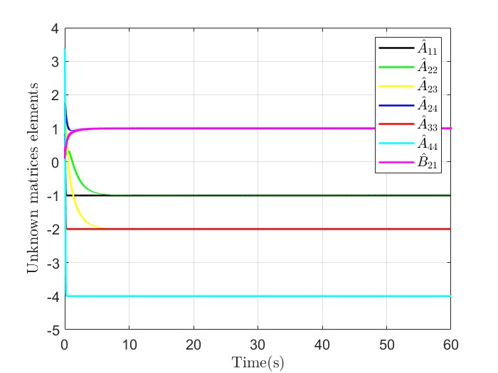
Figure 6: Estimated unknown elements of $A^{*}$ and $B^{*}$ with the library of observables $\theta=\{1,2,4,9\}$. Note that for simplicity of demonstration, we only show a non-zero elements of matrices.

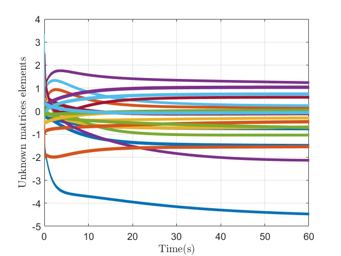
Figure 7: Estimated unknown elements of $A^{*}$ and $B^{*}$ with the library of observables $\theta=\{1,2,4,8\}$.

Example 2:

The vehicle is modeled as a nonlinear single-track bicycle model (See Fig. 8). The yaw dynamics of a simple vehicle can be qualitatively described and analyzed with this model in all operating conditions. Using the Lagrangian approach, the state equation of this vehicle model can be written as [Andrzejewski and Awrejcewicz, 2006, de Souza Mendes et al., 2016]

(144)

where the longitudinal forces acting on the front and rear tires, respectively, are given by ${F_{x,\mathbf{F}}}$ and ${F_{x,\mathbf{R}}}$. Moreover, ${F_{y,\mathbf{F}}}$ and ${F_{y,\mathbf{R}}}$ (the lateral forces) are also determined by the selected tire model where the subscripts _F and _R are denotes the front and rear points to which theses forces are associated. Moreover, ${\alpha_{T}}$ denotes the slip angle, and ${v_{T}}$ denotes the vehicle center of gravity velocity, ${m_{T}}$ denotes the vehicle mass, $\delta$ denotes the front axle steering angle, ${I_{T}}$ is the vehicle inertia, and the distances between the points $\mathbf{F}$ , CG, and $\mathbf{R}$ are determined by the constants $a$ and $b$.

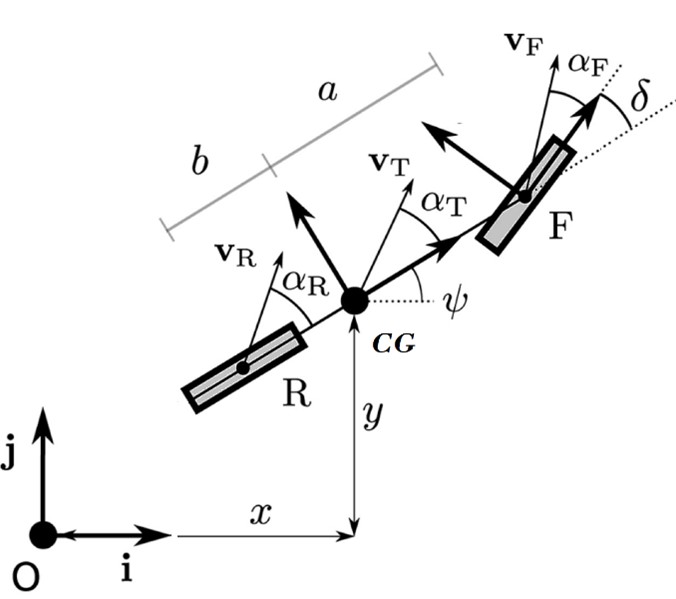
Figure 8: The single-track model. In this simulation, all tires on the same axle are assumed to have equal slip angles, and each axle is represented by a single tire with equivalent dynamic properties.

The following equation describes tire model

$${{{F}}_{{y,\mathbf{F}}}}=K{{\alpha}_{\mathbf{F}}},$$

$${{{F}}_{{y,\mathbf{R}}}}=K{{\alpha}_{\mathbf{R}}},$$ (145)

where the constant $K$ is stiffness, and

$$\begin{array}[]{l}{{\alpha}_{\mathbf{F}}}={\alpha_{\rm{T}}}+\frac{a}{{{v_{{\rm{T}},0}}}}\dot{\psi}-\delta,\\ {{\alpha}_{\mathbf{R}}}={\alpha_{\rm{T}}}-\frac{b}{{{v_{{\rm{T}},0}}}}\dot{\psi}.\end{array}$$ (148)

We first reformulate the vehicle dynamics (144) into nonlinear affine in control system and then develop a novel hierarchical learning structure that leverages a novel incremental finite-time Koopman-based update law to approximately learn the linear representation of vehicle dynamics (144). To this aim, using the facts that

$$\begin{array}[]{l}\cos({\alpha_{\rm{T}}}-\delta)=\cos{\alpha_{\rm{T}}}\cos\delta+\sin{\alpha_{\rm{T}}}\sin\delta,\\ \sin({\alpha_{\rm{T}}}-\delta)=\sin{\alpha_{\rm{T}}}\cos\delta-\cos{\alpha_{\rm{T}}}\sin\delta.\end{array}$$

One can rewrite (144) as

$$\begin{array}[]{l}{{\dot{v}}_{\rm{T}}}=\frac{2}{{{m_{T}}}}K{\alpha_{\rm{T}}}^{2}+\frac{1}{{{m_{T}}}}K\frac{{(a-b)}}{{{v_{{\rm{T}},0}}}}\dot{\psi}{\alpha_{\rm{T}}}-\frac{1}{{{m_{T}}}}K{\alpha_{\rm{T}}}\delta-(\frac{1}{{2{m_{T}}}}K{\alpha_{\rm{T}}}^{2}+\frac{1}{{2{m_{T}}}}K\frac{a}{{{v_{{\rm{T}},0}}}}\dot{\psi}{\alpha_{\rm{T}}}){\delta^{2}}+\frac{1}{{2{m_{T}}}}K{\alpha_{\rm{T}}}{\delta^{3}}\\ \,\,\,\,\,\,\,\,+(\frac{1}{{{m_{T}}}}K\frac{a}{{{v_{{\rm{T}},0}}}}\dot{\psi}\frac{{{\alpha_{\rm{T}}}^{2}}}{2}-\frac{1}{{{m_{T}}}}K\frac{a}{{{v_{{\rm{T}},0}}}}\dot{\psi}-\frac{1}{{{m_{T}}}}K{\alpha_{\rm{T}}}+\frac{1}{{{m_{T}}}}K{\alpha_{\rm{T}}}\frac{{{\alpha_{\rm{T}}}^{2}}}{2})\sin\delta+(\frac{1}{{{m_{T}}}}K-\frac{1}{{{m_{T}}}}K\frac{{{\alpha_{\rm{T}}}^{2}}}{2})\delta\sin\delta\\ {{\dot{\alpha}}_{\rm{T}}}=\frac{2}{{{m_{T}}{v_{\rm{T}}}}}K{\alpha_{\rm{T}}}+\frac{1}{{{m_{T}}{v_{\rm{T}}}}}K\frac{{(a-b)}}{{{v_{{\rm{T}},0}}}}\dot{\psi}-\frac{1}{{{m_{T}}{v_{\rm{T}}}}}K\frac{{(a-b)}}{{{v_{{\rm{T}},0}}}}\dot{\psi}\frac{{{\alpha_{\rm{T}}}^{2}}}{2}-\frac{2}{{{m_{T}}{v_{\rm{T}}}}}K\frac{{{\alpha_{\rm{T}}}^{3}}}{2}-\dot{\psi}+(\frac{1}{{{m_{T}}{v_{\rm{T}}}}}K\frac{{{\alpha_{\rm{T}}}^{2}}}{2}-\frac{1}{{{m_{T}}{v_{\rm{T}}}}}K)\delta\\ \,\,\,\,\,\,\,+(\frac{1}{{2{m_{T}}{v_{\rm{T}}}}}K{\alpha_{\rm{T}}}\frac{{{\alpha_{\rm{T}}}^{2}}}{2}-\frac{1}{{2{m_{T}}{v_{\rm{T}}}}}K\frac{a}{{{v_{{\rm{T}},0}}}}\dot{\psi}+\frac{1}{{2{m_{T}}{v_{\rm{T}}}}}K\frac{a}{{{v_{{\rm{T}},0}}}}\dot{\psi}\frac{{{\alpha_{\rm{T}}}^{2}}}{2}-\frac{1}{{2{m_{T}}{v_{\rm{T}}}}}K{\alpha_{\rm{T}}}){\delta^{2}}\\ \,\,\,\,\,\,\,+(\frac{1}{{2{m_{T}}{v_{\rm{T}}}}}K-\frac{1}{{{m_{T}}{v_{\rm{T}}}}}K\frac{{{\alpha_{\rm{T}}}^{2}}}{4}){\delta^{3}}+(\frac{1}{{{m_{T}}{v_{\rm{T}}}}}K{\alpha_{\rm{T}}}^{2}+\frac{1}{{{m_{T}}{v_{\rm{T}}}}}K\frac{a}{{{v_{{\rm{T}},0}}}}\dot{\psi}{\alpha_{\rm{T}}})\sin\delta-\frac{1}{{{m_{T}}{v_{\rm{T}}}}}K{\alpha_{\rm{T}}}\delta\sin\delta\\ \ddot{\psi}=\frac{1}{{{I_{T}}}}K{\alpha_{\rm{T}}}(a-b)+\frac{1}{{{I_{T}}}}K\frac{{({a^{2}}+{b^{2}})}}{{{v_{{\rm{T}},0}}}}\dot{\psi}-\frac{1}{{{I_{T}}}}K\delta a-(\frac{1}{{2{I_{T}}}}K\frac{{{a^{2}}}}{{{v_{{\rm{T}},0}}}}\dot{\psi}+\frac{1}{{2{I_{T}}}}K{\alpha_{\rm{T}}}a){\delta^{2}}+\frac{1}{{2{I_{T}}}}Ka{\delta^{3}}\end{array}$$ (156)

Observing the facts that $\sin\theta\approx\theta$ for $\theta\leq{13.99^{o}}$ and $\cos\theta\approx 1-{{{{(\theta)}^{2}}}\mathord{\left/{\vphantom{{{{(\theta)}^{2}}}2}}\right.\kern-1.2pt}2}$ for $\theta\leq{37.93^{\circ}}$ and the facts that ${0^{\circ}}\leq{\alpha_{\rm{T}}}\leq{10^{\circ}}$ for race and high-performance tires and the number is a little lower for street tires, and assuming $\left|\delta\right|\leq{35^{\circ}}$, and some manipulations, (156) can be rewritten into the following affine in control form

$$\begin{array}[]{l}\dot{X}=\left[{\begin{array}[]{*{20}{c}}{{{\dot{v}}_{\rm{T}}}}\\ {{{\dot{\alpha}}_{\rm{T}}}}\\ {\ddot{\psi}}\end{array}}\right]=\underbrace{\left[{\begin{array}[]{*{20}{c}}{\frac{2}{{{m_{T}}}}K{\alpha_{\rm{T}}}^{2}+\frac{1}{{{m_{T}}}}K\frac{{(a-b)}}{{{v_{{\rm{T}},0}}}}\dot{\psi}{\alpha_{\rm{T}}}}\\ {\frac{2}{{{m_{T}}{v_{\rm{T}}}}}K{\alpha_{\rm{T}}}+\frac{1}{{{m_{T}}{v_{\rm{T}}}}}K\frac{{(a-b)}}{{{v_{{\rm{T}},0}}}}\dot{\psi}-\frac{1}{{{m_{T}}{v_{\rm{T}}}}}K\frac{{(a-b)}}{{{v_{{\rm{T}},0}}}}\dot{\psi}\frac{{{\alpha_{\rm{T}}}^{2}}}{2}-\frac{2}{{{m_{T}}{v_{\rm{T}}}}}K\frac{{{\alpha_{\rm{T}}}^{3}}}{2}-\dot{\psi}}\\ {\frac{1}{{{I_{T}}}}K{\alpha_{\rm{T}}}(a-b)+\frac{1}{{{I_{T}}}}K\frac{{({a^{2}}+{b^{2}})}}{{{v_{{\rm{T}},0}}}}\dot{\psi}}\end{array}}\right]}_{{\cal I}(.)}\\ +\underbrace{\left[{\begin{array}[]{*{20}{c}}{\begin{array}[]{*{20}{c}}{{{\cal G}_{11}}}\\ {{{\cal G}_{21}}}\\ {{{\cal G}_{31}}}\end{array}}&{\begin{array}[]{*{20}{c}}{{{\cal G}_{12}}}\\ {{{\cal G}_{22}}}\\ {{{\cal G}_{32}}}\end{array}}&{\begin{array}[]{*{20}{c}}{{{\cal G}_{13}}}\\ {{{\cal G}_{23}}}\\ {{{\cal G}_{33}}}\end{array}}&{\begin{array}[]{*{20}{c}}{\begin{array}[]{*{20}{c}}{{{\cal G}_{14}}}\\ {{{\cal G}_{24}}}\\ {{{\cal G}_{34}}}\end{array}}&{\begin{array}[]{*{20}{c}}{{{\cal G}_{15}}}\\ {{{\cal G}_{25}}}\\ {{{\cal G}_{35}}}\end{array}}\end{array}}\end{array}}\right]}_{{\cal G}(.)}\underbrace{\left[{\begin{array}[]{*{20}{c}}\delta\\ {\sin\delta}\\ {\delta\sin\delta}\\ {\begin{array}[]{*{20}{c}}{{\delta^{2}}}\\ {{\delta^{3}}}\end{array}}\end{array}}\right]}_{{\cal U}(.)}\end{array}$$ (188)

where ${{{\cal G}_{11}}=\frac{{-K{\alpha_{\rm{T}}}}}{{{m_{T}}}}}$, ${{{\cal G}_{12}}=\frac{{-Ka}}{{{m_{T}}{v_{{\rm{T}},0}}}}\dot{\psi}+\frac{{Ka{\alpha_{\rm{T}}}^{2}}}{{2{m_{T}}{v_{{\rm{T}},0}}}}\dot{\psi}-\frac{{K{\alpha_{\rm{T}}}}}{{{m_{T}}}}+\frac{{K{\alpha_{\rm{T}}}^{3}}}{{2{m_{T}}}}}$, ${{{\cal G}_{13}}=\frac{K}{{{m_{T}}}}-\frac{{K{\alpha_{\rm{T}}}^{2}}}{{2{m_{T}}}}}$, ${{{\cal G}_{14}}=\frac{{-K{\alpha_{\rm{T}}}^{2}}}{{2{m_{T}}}}-\frac{{Ka{\alpha_{\rm{T}}}}}{{2{m_{T}}{v_{{\rm{T}},0}}}}\dot{\psi}}$, ${{{\cal G}_{15}}=\frac{{K{\alpha_{\rm{T}}}}}{{2{m_{T}}}}}$, ${{{\cal G}_{21}}=\frac{{-K}}{{{m_{T}}{v_{\rm{T}}}}}+\frac{{K{\alpha_{\rm{T}}}^{2}}}{{2{m_{T}}{v_{\rm{T}}}}}}$, ${{{\cal G}_{22}}=\frac{{K{\alpha_{\rm{T}}}^{2}}}{{{m_{T}}{v_{\rm{T}}}}}+\frac{{Ka{\alpha_{\rm{T}}}}}{{{m_{T}}{v_{\rm{T}}}{v_{{\rm{T}},0}}}}\dot{\psi}}$, ${{{\cal G}_{23}}=-\frac{{K{\alpha_{\rm{T}}}}}{{{m_{T}}{v_{\rm{T}}}}}}$, ${{\cal G}_{24}}=\frac{{K{\alpha_{\rm{T}}}^{3}}}{{4{m_{T}}{v_{\rm{T}}}}}-\frac{{Ka}}{{2{m_{T}}{v_{\rm{T}}}{v_{{\rm{T}},0}}}}\dot{\psi}+\frac{{Ka{\alpha_{\rm{T}}}^{2}}}{{4{m_{T}}{v_{\rm{T}}}{v_{{\rm{T}},0}}}}\dot{\psi}-\frac{{K{\alpha_{\rm{T}}}}}{{2{m_{T}}{v_{\rm{T}}}}}$, ${{{\cal G}_{25}}=\frac{K}{{2{m_{T}}{v_{\rm{T}}}}}-\frac{{K{\alpha_{\rm{T}}}^{2}}}{{4{m_{T}}{v_{\rm{T}}}}}}$, ${{{\cal G}_{31}}=\frac{{-Ka}}{{{I_{T}}}}}$, ${{{\cal G}_{32}}=0}$, ${{{\cal G}_{33}}=0}$, ${{{\cal G}_{34}}=\frac{{-K{a^{2}}}}{{2{I_{T}}{v_{{\rm{T}},0}}}}\dot{\psi}-\frac{{K{\alpha_{\rm{T}}}a}}{{2{I_{T}}}}}$, and ${{{\cal G}_{35}}=\frac{{Ka}}{{2{I_{T}}}}}$. Moreover, ${\cal I}({\cal X})$, ${\cal G}({\cal X})$, and ${\cal U}(\delta)$ are the drift dynamics of the system, the control input, and the input dynamics of the system, respectively.

The vehicle model for this study is a nonlinear single-track bicycle given in (188) and shown in Fig. 8. It is noteworthy that this model is capable of qualitatively describing a simple nonlinear vehicle yaw dynamics in all operating conditions corresponding to $\left|{{\alpha_{\rm{T}}}}\right|\leq 0.174533\,\,rad$, $\left|\psi\right|\leq 0.3\,\,rad$, $\left|{\dot{\psi}}\right|\leq 0.7\,\,rad/{\mathop{\rm s}\nolimits}$, and $\left|\delta\right|\leq{37.93}^{\circ}$.

Table 1: Vehicle parameters.

Item	Value	Description
${{m_{T}}}$	1300.0 kg	Total mass
${{I_{T}}}$	${{{10}^{4}}}{{\rm{kg}}\cdot{{\rm{m}}^{2}}}$	Moment of inertia
${{K}}$	$4\times{{10}^{4}}$	Tires stiffness
$\alpha_{T,0}$	0 rad	Initial vehicle sideslip angle
$\dot{\Psi}_{0}$	0.01 $rad/s$	Initial yaw rate
${v}_{0}$	20 $m/s$	Initial velocity
$a$	1.6154	Distance to CG
$b$	1.8846	Distance to CG

Assuming that $v_{\rm{T}}\geq 1{m\mathord{\left/{\vphantom{ms}}\right.\kern-1.2pt}s}$, and let the observable functions consist of the elements of the state vector $\cal{X}$ as:

(191)

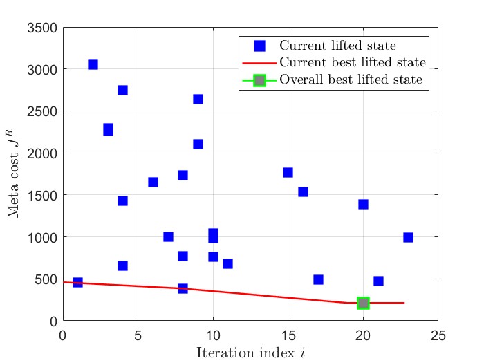
Figure 9: Meta cost $J^{R}$ vs iteration $i$ of Algorithm 1. At each iteration $i$, the cost of the current set of observable functions and of the current best one are depicted. The green square shows the overall best lifted state $\xi_{\theta}=[\psi,{\alpha_{T}},\dot{\psi},{\alpha_{T}}^{2},{\alpha_{\rm{T}}}^{3},\frac{{{\alpha_{T}}}}{{{v_{\rm{T}}}}},\frac{{{\alpha_{T}}^{2}}}{{{v_{\rm{T}}}}},\frac{{{\alpha_{T}}^{3}}}{{{v_{\rm{T}}}}},{\alpha_{T}}\dot{\psi},{\alpha_{\rm{T}}}^{2}\dot{\psi},\allowbreak\frac{1}{{{v_{\rm{T}}}}}\dot{\psi},\frac{{{\alpha_{T}}}}{{{v_{\rm{T}}}}}\dot{\psi},\frac{{{\alpha_{T}}^{2}}}{{{v_{\rm{T}}}}}\dot{\psi}]^{\top}$ which is found at iteration $20$.

The meta cost $J^{R}$ vs iteration $i$ of Algorithm 1 is illustrated in Fig. 9. Note that for the lifted state $\xi_{\theta}=[\psi,{\alpha_{T}},\dot{\psi},{\alpha_{T}}^{2},{\alpha_{\rm{T}}}^{3},\frac{{{\alpha_{T}}}}{{{v_{\rm{T}}}}},\frac{{{\alpha_{T}}^{2}}}{{{v_{\rm{T}}}}},\frac{{{\alpha_{T}}^{3}}}{{{v_{\rm{T}}}}},{\alpha_{T}}\dot{\psi},{\alpha_{\rm{T}}}^{2}\dot{\psi},\allowbreak\frac{1}{{{v_{\rm{T}}}}}\dot{\psi},\frac{{{\alpha_{T}}}}{{{v_{\rm{T}}}}}\dot{\psi},\frac{{{\alpha_{T}}^{2}}}{{{v_{\rm{T}}}}}\dot{\psi}]^{\top}$, one has

(202)

$$\begin{array}[]{l}{{\dot{v}}_{\rm{T}}}={\left[{0,0,0,\frac{{2K}}{{{m_{T}}}},0,0,0,0,\frac{{K(a-b)}}{{{m_{T}}{v_{{\rm{T}},0}}}},0,0,0,0}\right]^{\top}}{\xi_{\theta}}\\ \,\,\,\,\,\,+\left[{\begin{array}[]{*{20}{c}}{\begin{array}[]{*{20}{c}}{{{\bar{\cal G}}_{11}}}\\ 0\\ 0\\ {\begin{array}[]{*{20}{c}}0\\ 0\end{array}}\end{array}}&{\begin{array}[]{*{20}{c}}0\\ {{{\bar{\cal G}}_{12}}}\\ 0\\ {\begin{array}[]{*{20}{c}}0\\ 0\end{array}}\end{array}}&{\begin{array}[]{*{20}{c}}0\\ 0\\ {{{\bar{\cal G}}_{13}}}\\ {\begin{array}[]{*{20}{c}}0\\ 0\end{array}}\end{array}}&{\begin{array}[]{*{20}{c}}{\begin{array}[]{*{20}{c}}0\\ 0\\ 0\\ {\begin{array}[]{*{20}{c}}{{{\bar{\cal G}}_{14}}}\\ 0\end{array}}\end{array}}&{\begin{array}[]{*{20}{c}}0\\ 0\\ 0\\ {\begin{array}[]{*{20}{c}}0\\ {{{\bar{\cal G}}_{15}}}\end{array}}\end{array}}\end{array}}\end{array}}\right]({I_{5}}\otimes{\xi_{\theta}})\left[{\begin{array}[]{*{20}{c}}\delta\\ {\sin\delta}\\ {\delta\sin\delta}\\ {\begin{array}[]{*{20}{c}}{{\delta^{2}}}\\ {{\delta^{3}}}\end{array}}\end{array}}\right]\end{array}$$ (243)

where ${{\bar{\cal G}}_{11}}=\left[{0,\frac{{-K}}{{{m_{T}}}},0,0,0,0,0,0,0,0,0,0,0}\right]$, ${{\bar{\cal G}}_{12}}=\left[{0,\frac{{-K}}{{{m_{T}}}},\frac{{-Ka}}{{{m_{T}}{v_{{\rm{T}},0}}}},0,\frac{K}{{2{m_{T}}}},0,0,0,0,\frac{{Ka}}{{2{m_{T}}{v_{{\rm{T}},0}}}},0,0,0}\right]$, ${{\bar{\cal G}}_{13}}=\left[{0,\frac{K}{{{m_{T}}}},0,\frac{{-K}}{{2{m_{T}}}},0,0,0,0,0,0,0,0,0}\right]$, ${{\bar{\cal G}}_{14}}=\left[{0,0,0,\frac{{-K}}{{2{m_{T}}}},0,0,0,0,\frac{{-Ka}}{{2{m_{T}}{v_{{\rm{T}},0}}}},0,0,0,0}\right]$, and ${{\bar{\cal G}}_{15}}=\left[{0,\frac{K}{{2{m_{T}}}},0,0,0,0,0,0,0,0,0,0,0}\right]$.

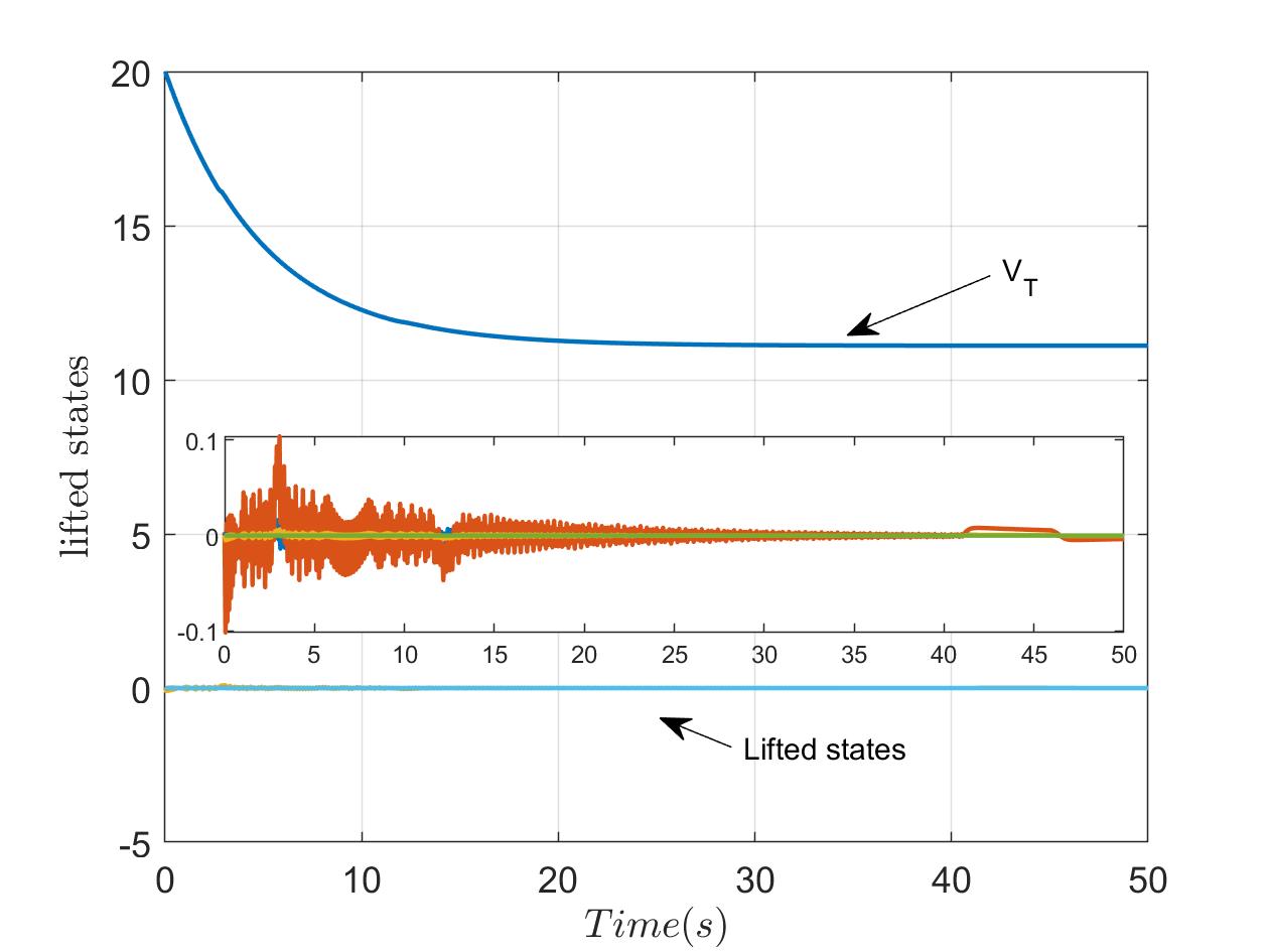
Figure 10: Evolution of the lifted state $\xi_{\theta}$ and $v_{T}$ trajectories.

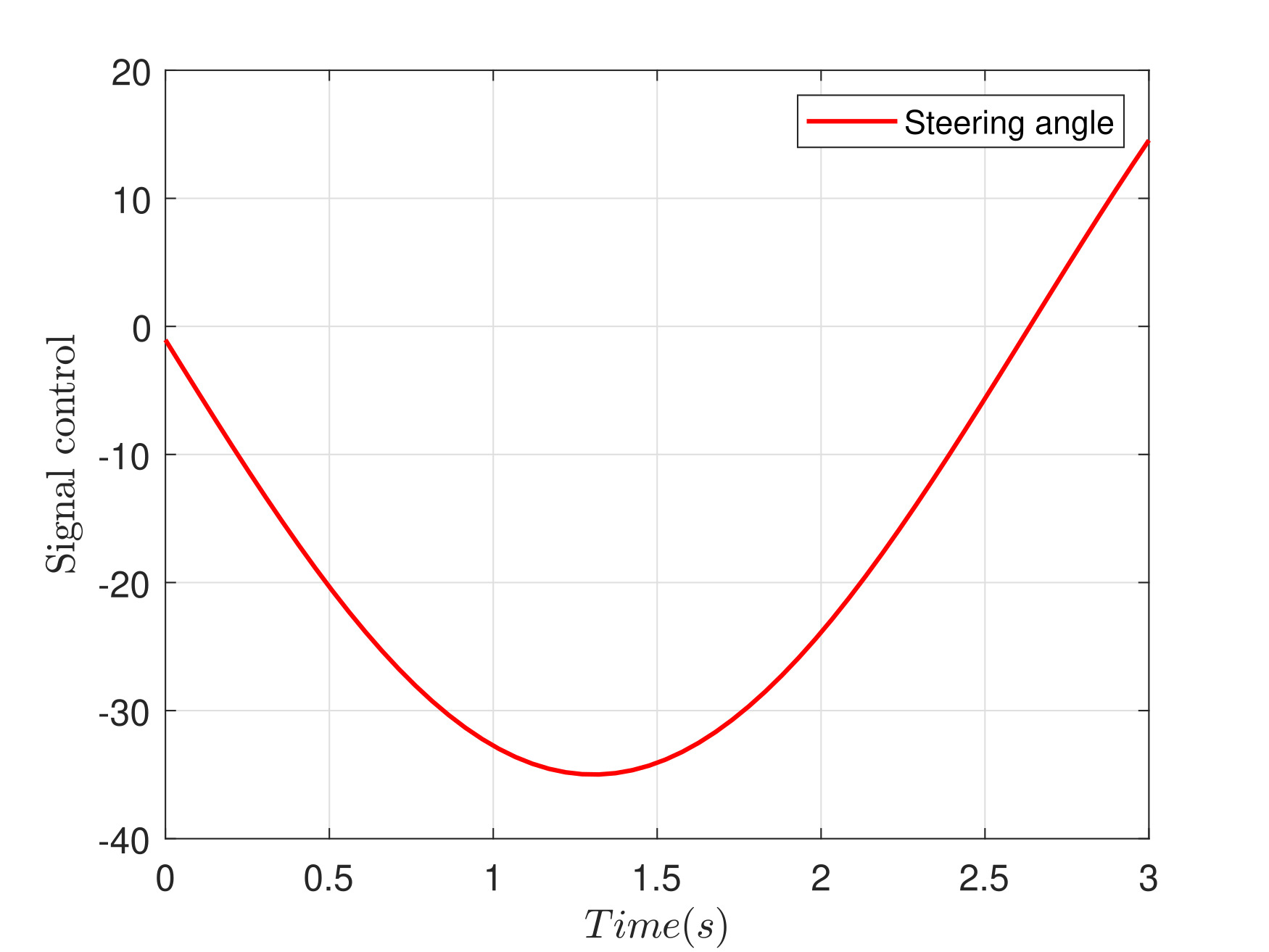
Figure 11: Control input $\delta=-35Sin(1.2t)$ Degree.

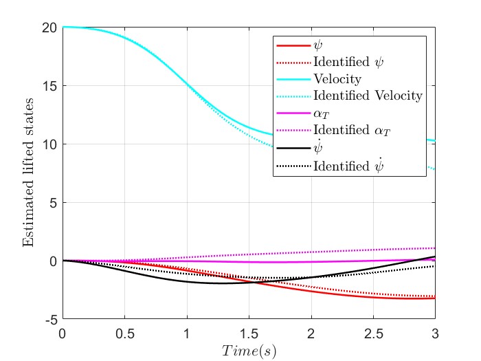
Figure 12: States trajectories of the nonlinear vehicle system and the identified model under control input of $\delta=-35Sin(1.2t)$ Degree.

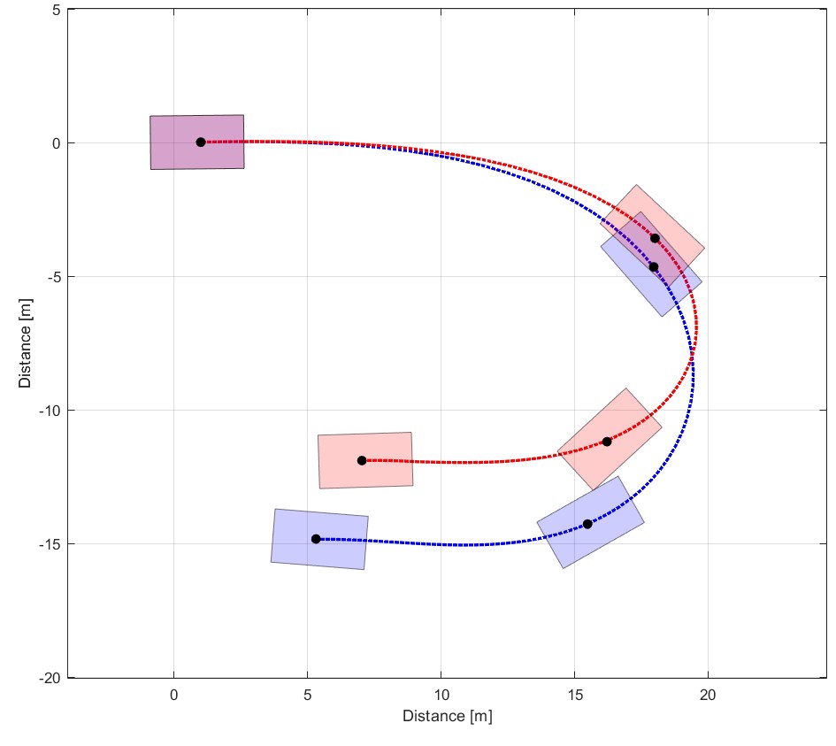
Figure 13: $X$ and $Y$ position trajectories of the nonlinear vehicle system (Light-Blue square) and the identified model (Light-Coral square) under control input of $\delta=-35Sin(1.2t)$ Degree.

To satisfy Condition 1, a rich enough input signal $\delta$ is injected into the nonlinear vehicle system (188) for excitation of the lifted states $\xi_{\theta}$. The evolution of the lifted states trajectories under the rich enough input signal $\delta$ is shown in Fig. 10. The proposed update law (42)-(44) is used to find the approximated matrices $\hat{A}^{*}_{\theta}$, and $\hat{B}^{*}_{\theta}$. After the convergence of $\hat{A}_{\theta}^{*}$ and $\hat{B}_{\theta}^{*}$, the control input $\delta$, given in Fig. 11, is employed for the identified linear representation system (202) and the nonlinear vehicle system (188) to compare the evolution of the states trajectories of the identified model and the nonlinear vehicle system (188). Using the equations of motion [Andrzejewski and Awrejcewicz, 2006, de Souza Mendes et al., 2016]

(246)

Fig. 13, illustrates the comparison of $X-Y$ positions of the nonlinear vehicle system (188) and the identified model (202).

Now, to test the learned model, we assumed that a disturbance as a single steering pulse with the magnitude of $\delta=30^{\circ}$ is simulated at $t=0-0.2$ sec. The control input $\delta$ as depicted in Fig. 14 is employed for the nonlinear vehicle system (188) to stabilize the states $\{\psi,\alpha_{T},\dot{\psi}\}$. For the comparison, the feedback gain $K$ is also applied to the identified model. Fig. 15 depicts the evolution of state trajectories of identified (dashed line) and real (solid line) nonlinear system, which shows that the both state trajectories. Fig. 16, illustrates the comparison of $X-Y$ positions of the nonlinear vehicle system (11) and the identified model (102) under the control input given in Fig. 16.

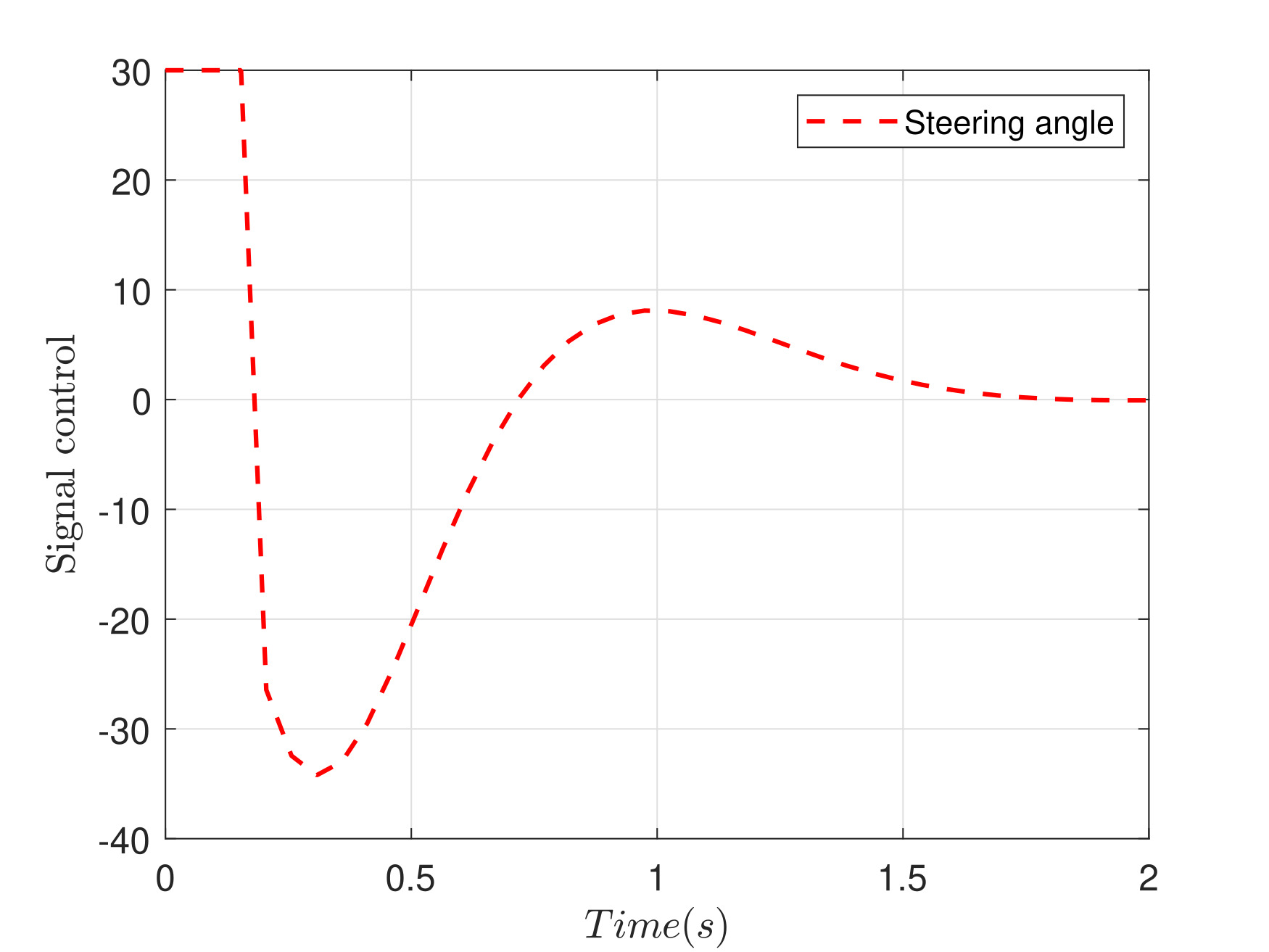
Figure 14: Control input $\delta$.

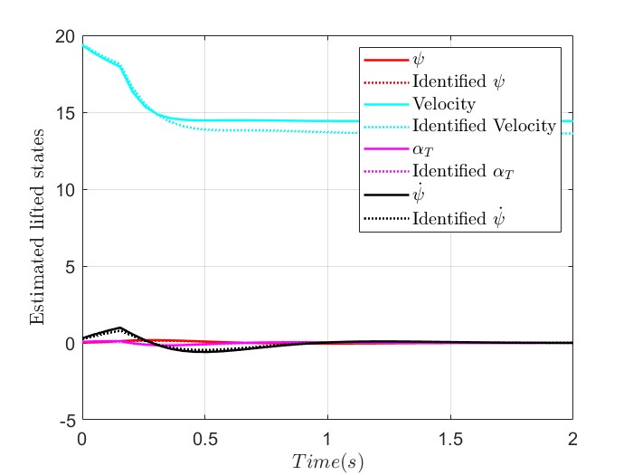
Figure 15: State trajectories of identified (dashed line) and real (solid line) nonlinear system with $\delta$.

Figure 16: $X$ and $Y$ position trajectories of the nonlinear vehicle system (Light-Blue square) and the identified model (Light-Coral square) with control input of $\delta$.

6 Conclusion

A novel data-driven learning algorithm is presented to learn a linear representation of nonlinear system dynamics using Koopman operator theory. To jointly learn the set of observables (structure) and Koopman parameters, a bilevel learning mechanism with two layers of learning is developed. The lower layer learner leverages unified batch-online learning-based finite-time Koopman identifier which uses discontinuous gradient update laws to minimize the instantaneous Koopman operator’s identification errors as well as the identification errors for a batch of past samples collected in a history stack. It is guaranteed that the lower layer identifier will converge in a finite time under easy-to-verify conditions on a batch of samples. A higher layer employs a discrete Bayesian optimization algorithm to find a set of observables with minimum approximation errors and minimum cardinality. Finally, the effectiveness of the proposed framework was verified on a simulation example.

Acknowledgments

This work was supported by Ford Motor Company-Michigan State University Alliance.

References

- Andrzejewski and Awrejcewicz [2006] Ryszard Andrzejewski and Jan Awrejcewicz. Nonlinear dynamics of a wheeled vehicle, volume 10. Springer Science & Business Media, 2006.
- Ayoobi et al. [2021] Hamed Ayoobi, Ming Cao, Rineke Verbrugge, and Bart Verheij. Argumentation-based online incremental learning. IEEE Transactions on Automation Science and Engineering, pages 1–15, 2021.