The 3-D Kinematics of the Orion Nebula Cluster: NIRSPEC-AO Radial Velocities of the Core Population

Abstract

The kinematics and dynamics of stellar and substellar populations within young, still-forming clusters provides valuable information for constraining theories of formation mechanisms. Using Keck II NIRSPEC+AO data, we have measured radial velocities for 56 low-mass sources within 4′ of the core of the Orion Nebula Cluster (ONC). We also re-measure radial velocities for 172 sources observed with SDSS/APOGEE. These data are combined with proper motions measured using HST ACS/WFPC2/WFC3IR and Keck II NIRC2, creating a sample of 135 sources with all three velocity components. The velocities measured are consistent with a normal distribution in all three components. We measure intrinsic velocity dispersions of ($\sigma_{v_{\alpha}}$, $\sigma_{v_{\delta}}$, $\sigma_{v_{r}}$) = ($1.64\pm 0.12$, $2.03\pm 0.13$, $2.56^{+0.16}_{-0.17}$) km s^-1. Our computed intrinsic velocity dispersion profiles are consistent with the dynamical equilibrium models from Da Rio et al. (2014) in the tangential direction, but not in the line of sight direction, possibly indicating that the core of the ONC is not yet virialized, and may require a non-spherical potential to explain the observed velocity dispersion profiles. We also observe a slight elongation along the north-south direction following the filament, which has been well studied in previous literature, and an elongation in the line of sight to tangential velocity direction. These 3-D kinematics will help in the development of realistic models of the formation and early evolution of massive clusters.

1 Introduction

The Orion Nebula Cluster (ONC) represents one of the best laboratories for studies of cluster formation and dynamics. Since the vast majority of stars are expected to form in clusters (Allen, 2007; Carpenter, 2000; Lada & Lada, 2003), understanding cluster formation is of paramount importance to constraining star formation theory. The ONC is one of the closest ($d\approx 390$ pc; Kounkel et al., 2017) examples of massive star formation, covering a large range of source masses (0.1–50 $M_{\sun}$ Hillenbrand, 1997). There is also evidence to suggest that the cluster is not yet dynamically relaxed (Fűrész et al., 2008; Tobin et al., 2009), which is consistent with its youth ($\sim$2.2 Myr; Reggiani et al., 2011).

Early studies of the kinematics of the ONC identified mass segregation, which is expected for young clusters (Hillenbrand, 1997; Hillenbrand & Hartmann, 1998). However, it remains an open question as to whether the observed mass segregation is primordial or dynamical. Given the estimated age of the ONC ($\sim$2.2 Myr), and the cluster crossing time ($\sim$2 Myr), it is thought that the mass segregation is primordial (Reggiani et al., 2011). However, these studies relied on a limited sample of 3-D kinematic information, largely resulting from the high level of extinction in the region (e.g., Johnson, 1965; Walker, 1983; Jones & Walker, 1988; van Altena et al., 1988).

The largest scale radial velocity (RV) studies of the ONC began with Fűrész et al. (2008) and Tobin et al. (2009), who observed 1215 and 1613 stars, respectively. These observations were taken using the Hectochelle multiobject echelle spectrograph (Szentgyorgyi et al., 1998) on the 6.5-m MMT telescope, and the Magellan Inamori Kyocera Echelle (MIKE; Bernstein et al., 2003; Walker et al., 2007) on the Magellan Clay telescope. These fiber-fed instruments obtain high-resolution ($\lambda/\Delta\lambda\approx 35,000$), optical (5150–5300 Å) spectra, but are limited in their ability to observe stars in highly embedded regions and/or crowded fields (minimum separations of 30″ for Hectochelle and 14″ for MIKE). In particular, the core of the ONC—within 1′ of the Trapezium—had poor coverage (5 sources) due to the highly embedded and crowded nature of the core.

More recently, the Sloan Digital Sky Survey (SDSS; York et al., 2000), SDSS-III (Eisenstein et al., 2011) Apache Point Observatory Galactic Evolution Experiment (APOGEE; Majewski et al., 2017) conducted an infrared (IR) survey of the ONC (Da Rio et al., 2016, 2017). The APOGEE spectrograph (Wilson et al., 2010) on the Sloan 2.5-m telescope (Gunn et al., 1998) is a fiber-fed instrument which obtains $H$-band spectra (1.51–1.68 $\mu$m) at a resolution of $\lambda/\Delta\lambda\approx 22,500$. This makes surveys using the APOGEE spectrograph less affected by extinction in embedded regions, but they are still limited in their ability to observe objects in crowded regions due to the 2″ diameter fibers. The most recent compilation of APOGEE measurements (APOGEE-II) was given in Kounkel et al. (2018, hereafter K18), which included measurements from SDSS Data Release 12 (DR12; Alam et al., 2015) and Data Release 14 (DR14; Abolfathi et al., 2018). K18 presented high-precision ($\sim$0.2 km s^-1) RVs for 7774 sources in the ONC, but only included 12 sources within 1′ of the Trapezium.

Here, we present a study of the 3-D kinematics of the ONC sources within 4′ of the Trapezium. Our sample consists of 56 sources observed with the Near InfarRed echelle SPECtrograph (NIRSPEC; McLean et al., 1998, 2000) on the Keck II 10-meter telescope coupled with adaptive optics (AO), and a reanalysis of 172 sources observed with SDSS/APOGEE. This combined ONC sample represents the largest sample to date of RVs within the core of the ONC ($\lesssim 1\arcmin$; 41 sources). In Section 2, we discuss the literature data and new observations used in this study. Section 3 describes the methods used in reducing and forward-modeling the NIRSPEC+AO (NIRSPAO) data. We discuss a reanalysis of the SDSS/APOGEE data using our forward-modeling pipeline in Section 4. A detailed study of the 3-D kinematics of the ONC core is undertaken in Section 5. Lastly, a discussion of our results is given in Section 6.

2 Data

We obtained high-resolution near-infrared (NIR) spectra of sources closest to the core of the ONC—surrounding the Trapezium—using Keck/NIRSPAO between 2015–2020. Targets were initially chosen from a preliminary catalog of proper motions (PMs) computed using Keck Near Infrared Camera 2 (NIRC2; PI: K. Matthews) data. These sources were then cross-referenced with the Hillenbrand & Carpenter (2000) study of the low-mass members of the ONC. Figure 1 shows the targets from this study, as well as sources with RVs from the optical survey of Tobin et al. (2009, hereafter T09) and the NIR survey using SDSS/APOGEE presented in Kounkel et al. (2018, hereafter K18). For the remainder of this study, we use the center-of-mass (CoM) coordinates determined by Da Rio et al. ($\alpha_{\mathrm{J2000}}=05$:35:16.26; $\delta_{\mathrm{J2000}}=-05$:23:16.4; 2014) to represent the “center” of the ONC.

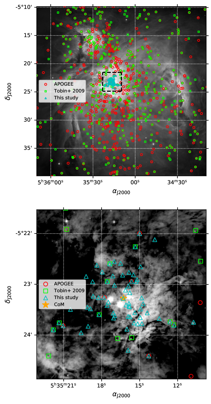
Figure 1: Top: HST ACS $R$-band image of the ONC (Robberto et al., 2013). Plotted are K18 APOGEE sources (red circles), T09 sources (green squares), and NIRSPAO sources from this study (cyan triangles). The black dashed box indicates the area shown in the bottom figure. Bottom: Close up image of the Trapezium. Sources are plotted with markers indicated in the legend. Our sources primarily represent the reddest sources closest to the Trapezium. The center-of-mass coordinates from Da Rio et al. (2014) are indicated with the orange star.

2.1 NIRSPAO Observations

All objects in our curated sample were observed using NIRSPEC on Keck II, in conjunction with the laser guide star (LGS) adaptive optics (AO) system (van Dam et al., 2006; Wizinowich et al., 2006). We used the instrument in its high-spectral resolution AO mode with a slit width $\times$ slit length of $0.041\arcsec\times 2.26\arcsec$. Observations were carried out in the $K$- or $N7$-band to capitalize on the strong CO bands within that regime ($\sim$2.3 $\mu$m, orders 32 & 33). We additionally used a cross-disperser angle of 35.65^∘ and an echelle angle of 63^∘. The resolution in this setup is $R\approx$ 25,000, as determined by the width of unresolved OH sky lines, and the wavelengths covered are approximately 2.044–2.075 $\mu$m (order 37), 2.100–2.133 $\mu$m (order 36), 2.160–2.193 $\mu$m (order 35), 2.224–2.256 $\mu$m (order 34), 2.291–2.325 $\mu$m (order 33), and 2.362–2.382 $\mu$m (order 32), with some portions of the bands beyond the edges of the detector. For this work, all analysis was done using orders 32 and 33, the orders containing the CO bandheads in addition to numerous telluric features, and all NIRSPAO data presented come from these orders. We note that NIRSPEC underwent an upgrade during 2018, and our setup changed slightly post-upgrade. The most significant change is a larger wavelength coverage for each order due to a larger Hawaii 2RG detector ($2048\times 2048$ post-upgrade versus $1024\times 1024$ pre-upgrade; Martin et al. 2018), and a higher resolution ($R\approx$ 35,000; Hsu et al., 2021b).

Typical observations consisted of four spectra taken in an ABBA dither pattern along the length of the slit. In a few cases, more or less than four spectra were taken. Either before or after each target was observed, an A0V calibrator star at similar airmass was observed for a telluric reference. Table 1 gives the log of our spectroscopic observations, listing the targets observed, the date of observation, the number of spectra, and the integration time for each spectrum. Etalon lamp and flat field frames were also taken each night for use in data reduction (Section 3).

Table 1: Log of NIRSPAO-LGS Observations

Target	Date of	A0V Star	Exposure Time	No. of	Filter
Name	Obs. (UT)	Standard	(s $\times$ coadds)	Frames
HC322	2015 Dec 23	HD 37887	$300\times 1$	4	$K$
HC296	2015 Dec 23	HD 37887	$1200\times 1$	4	$K$
HC259	2015 Dec 23	HD 37887	$90\times 1$	4	$K$
HC213	2015 Dec 23	HD 37887	$60\times 1$	4	$K$
HC306	2015 Dec 24	HD 37887	$180\times 1$	4	$K$
HC287	2015 Dec 24	HD 37887	$600\times 1$	4	$K$
HC291	2015 Dec 24	HD 37887	$600\times 1$	4	$K$
HC252	2015 Dec 24	HD 37887	$300\times 1$	4	$K$
HC250	2015 Dec 24	HD 37887	$1200\times 1$	4	$K$
HC244	2015 Dec 24	HD 37887	$600\times 1$	4	$K$
HC261	2015 Dec 24	HD 37887	$900\times 1$	4	$K$
HC248	2016 Dec 14	HD 37887	$600\times 1$	4	$K$
HC223	2016 Dec 14	HD 37887	$300\times 1$	4	$K$
HC219	2016 Dec 14	HD 37887	$600\times 1$	4	$K$
HC324	2016 Dec 14	HD 37887	$1200\times 1$	3	$K$
HC295	2018 Feb 11	HD 37887	$450\times 1$	5	$K$
HC313	2018 Feb 11	HD 37887	$180\times 1$	4	$K$
HC332	2018 Feb 11	HD 37887	$300\times 1$	4	$K$
HC331	2018 Feb 11	HD 37887	$450\times 1$	4	$K$
HC337	2018 Feb 11	HD 37887	$60\times 1$	4	$K$
HC375	2018 Feb 11	HD 37887	$180\times 1$	4	$K$
HC338	2018 Feb 11	HD 37887	$120\times 1$	4	$K$
HC425	2018 Feb 12	HD 37887	$60\times 1$	4	$K$
HC713	2018 Feb 12	HD 37887	$90\times 1$	4	$K$
HC408	2018 Feb 12	HD 37887	$450\times 1$	4	$K$
HC410	2018 Feb 12	HD 37887	$600\times 1$	4	$K$
HC436	2018 Feb 12	HD 37887	$90\times 1$	4	$K$
HC442	2018 Feb 13	HD 37887	$450\times 1$	4	$K$
HC344	2018 Feb 13	HD 37887	$60\times 1$	4	$K$
HC522	2019 Jan 12	HD 37887	$450\times 1$	4	$K$
HC145	2019 Jan 12	HD 37887	$600\times 1$	4	$K$
HC202	2019 Jan 12	HD 37887	$120\times 1$	4	$K$
HC188	2019 Jan 12	HD 37887	$600\times 1$	4	$K$
HC302	2019 Jan 13	HD 37887	$450\times 1$	4	$N7$
HC275	2019 Jan 13	HD 37887	$450\times 1$	2	$N7$
HC245	2019 Jan 13	HD 37887	$180\times 1$	4	$N7$
HC258	2019 Jan 13	HD 37887	$180\times 1$	4	$N7$
HC344	2019 Jan 13	HD 37887	$120\times 1$	4	$N7$
HC370	2019 Jan 16	HD 37887	$180\times 1$	4	$N7$
HC389	2019 Jan 16	HD 37887	$120\times 1$	4	$N7$
HC386	2019 Jan 16	HD 37887	$120\times 1$	4	$N7$
HC398	2019 Jan 16	HD 37887	$120\times 1$	4	$N7$
HC413	2019 Jan 16	HD 37887	$180\times 1$	4	$N7$
HC253	2019 Jan 16	HD 37887	$120\times 1$	4	$N7$
HC288	2019 Jan 17	HD 37887	$450\times 1$	4	$N7$
HC420	2019 Jan 17	HD 37887	$450\times 1$	4	$N7$
HC412	2019 Jan 17	HD 37887	$450\times 1$	4	$N7$
HC288	2019 Jan 17	HD 37887	$450\times 1$	4	$N7$
HC282	2019 Jan 17	HD 37887	$450\times 1$	3	$N7$
HC277	2019 Jan 17	HD 37887	$180\times 1$	4	$N7$
HC217	2020 Jan 18	HD 37887	$120\times 1$	4	$N7$
HC229	2020 Jan 18	HD 37887	$450\times 1$	4	$N7$
HC229	2020 Jan 18	HD 37887	$450\times 1$	4	$N7$
HC228	2020 Jan 19	HD 37887	$120\times 1$	4	$N7$
HC224	2020 Jan 19	HD 37887	$90\times 1$	4	$N7$
HC135	2020 Jan 19	HD 37887	$180\times 1$	4	$N7$
HC440	2020 Jan 20	HD 37887	$120\times 1$	4	$N7$
HC450	2020 Jan 20	HD 37887	$300\times 1$	4	$N7$
HC277	2020 Jan 20	HD 37887	$300\times 1$	4	$N7$
HC204	2020 Jan 20	HD 37887	$300\times 1$	4	$N7$
HC229	2020 Jan 20	HD 37887	$450\times 1$	4	$N7$
HC214	2020 Jan 20	HD 37887	$450\times 1$	4	$N7$
HC215	2020 Jan 21	HD 37887	$300\times 1$	4	$N7$
HC240	2020 Jan 21	HD 37887	$300\times 1$	4	$N7$
HC546	2020 Jan 21	HD 37887	$300\times 1$	4	$N7$
HC504	2020 Jan 21	HD 37887	$120\times 1$	4	$N7$
HC703	2020 Jan 21	HD 37887	$300\times 1$	4	$N7$
HC431	2020 Jan 21	HD 37887	$120\times 1$	3	$N7$
HC229	2020 Jan 21	HD 37887	$450\times 1$	2	$N7$

3 NIRSPAO Reduction

Reduction of NIRSPAO data was done using a modified version of the NIRSPEC Data Reduction Pipeline (NSDRP). The NSDRP was specifically designed for point source extraction, and has been used extensively to obtain “quick looks” while observing at the Keck facility and for the Keck Observatory Archive (KOA; Berriman et al., 2005, 2010; Tran et al., 2012). Our updated version includes the following modifications:

1. Use with the $K$-AO observing mode.

2. Spatial rectification using the object trace rather than the order edge traces.

3. Spectral rectification and wavelength calibration using etalon lamps.

4. Cosmic ray cleaning of flats.

5. Bad pixel cleaning using methods ported from fixpix_rs.pro which is a utility from REDSPEC (Kim et al., 2015; Prato et al., 2015).

In addition to the above modifications, we also removed fringes from the flat field images prior to median combining using the wavelet method of Rojo & Harrington (2006). This helps to mitigate beat patterns that can appear between fringing in the flats and science data.

Data for each night was reduced using standard procedures following the NSDRP documentation. We provide a summary of the steps involved in the reduction process here.

1. Flat frames are median combined into a master flat frame.

2. The master flat is used to find order edges using pre-determined dispersions based on the grating equation for NIRSPEC.

3. Each frame (i.e., object, etalon/arc lamp) is cleaned for cosmic rays using Laplacian edge detection (van Dokkum, 2001).

4. Each frame is flat normalized and orders are extracted individually using the edges traces found from the master flat frame.

5. Each order is cleaned for bad pixels using the fixpix routine.

6. Each order is spatially rectified using the object trace, determined by a Gaussian profile fit along each column.

7. Order edges are trimmed to remove bad pixels.

8. Each order is spectrally rectified using either the etalon or the arc lamp frame. The spectral trace is done by fitting Gaussians to the emission line traces, and then finding the optimal spectral tilt (y-direction).

9. The object is extracted using box extraction, using optimal object and background regions found from Gaussian fits to the profile. The average sky (calculated using background regions adjacent to the 2-D object spectrum) is subtracted from the object spectrum.

10. Flux and noise are calculated using standard methods in the NSDRP.

11. The wavelength solution is calibrated for each order using a synthesized etalon or sky spectrum and fitting to lines found in each order.

Initial wavelength solutions were obtained by mapping pixels to the etalon lamp wavelengths; however, etalon lamps only provide uniform spacing in the frequency domain, with the initial absolute or starting position unknown. For example, it is unknown whether the first etalon fringe starts at 20000 Å or 20010 Å  but the spacing of $c\lambda^{-1}$ is absolute. Therefore, the wavelength solution is re-calibrated using telluric features within each frame, which are anchored to an absolute rest-frame, as part of our forward-modeling framework (Section 3.1).

3.1 Forward-Modeling NIRSPEC Data

Our data were forward-modeled using the Spectral Modeling Analysis and RV Tool (SMART; Hsu et al., 2021a). Details for the fitting routine using SMART are given in Hsu et al. (2021b). Here, we briefly outline our methods.

Reduced NIRSPAO data were modeled using an iterative approach. The first step was obtaining an absolute wavelength solution to orders 32 and 33. For our initial wavelength solution, we use the global wavelength solution provided by the NSDRP—which is a quadratic polynomial of the form

$$\lambda(p,M)=r_{0}+r_{1}p+r_{2}p^{2}+\frac{r_{3}}{M}+\frac{r_{4}p}{M}+\frac{r_{5}p^{2}}{M},$$ (1)

where $\lambda(p,M)$ is the wavelength falling on column pixel $p$ of order $M$ and coefficients $r_{n}$. This initial wavelength solution is obtained from fitting to the etalon lamps, which provides uniform offsets in frequency space. However, as mentioned previously, the absolute wavelength solution, or starting position, is unknown for the etalon spectrum.

To obtain a more precise a wavelength calibration, we performed a cross-correlation between our telluric spectrum from the A-star calibrator to the high-resolution telluric spectrum from Moehler et al. (2014). First, we modeled and removed the continuum of our A-star calibrator using a quadratric polynomial, essentially leaving just the flat imprinted telluric absorption spectrum. Then, we scaled the flux of the high-resolution telluric model to the A-star flux. Next, the telluric spectrum from the A0V star was cross-correlated with the telluric model using a window of 100 pixels, and a step size of 20 pixels, calculating the best fit cross-correlation shift for each window along the entire spectrum. Then, a 4th order polynomial—i.e., $\lambda(p)=a_{i}+b_{i}p+c_{i}p^{2}+d_{i}p^{3}+e_{i}p^{4}$, where $i$ is the iteration number—was fit to the best wavelength shifts for all windows used in that iteration. The initial wavelength solution was given using the 2nd order polynomial provided by the NSDRP, with the additional coefficients set to zero (i.e., $d_{0}$, $e_{0}$). The best-fit coefficients for each pass (e.g., $\delta_{a_{0}}$) were added to the previous solution, e.g., $a_{1}=a_{0}+\delta_{a_{1}}$, $b_{1}=b_{0}+\delta_{b_{1}}$. This loop was repeated until the wavelength solution converged to the smallest residuals between the telluric spectrum and telluric model. One thing to note is that different iterations used different pixel window and step sizes as finer granularity is required as the wavelength solution gets closer to the optimal fit. For instance, the second pass used a step size of 10 pixels and a window size of 150 pixels.

The aforementioned fitting procedure was done for each frame independently, resulting in an absolute wavelength solution for each frame. We cross-correlated a single A star frame to A star calibration data taken over 14 nights (both A and B nods), and found a RMS between frames of 0.004 Å (0.058 km s^-1). Although this systematic uncertainty is typically much smaller than our measurement uncertainty, we add this systematic in quadrature with our measurement uncertainties per frame.

Next, we modeled the spectrum using a forward-modeling approach based on the method provided by Blake et al. (2010) and also Butler et al. (1996); Blake et al. (2007, 2008, 2010), and Burgasser et al. (2016), utilizing a Markov Chain Monte Carlo (MCMC) method built on the emcee (Foreman-Mackey et al., 2013) to sample the parameter space.

The flux from the source can be modeled using the following equation,

$$F_{M}[p]={} C[p(\lambda)]\times$$ (2)

$$\left[\left(\left(M\left[p^{\ast}\left(\lambda\left[1+\frac{V_{r}}{c}\right]\right),\,T_{\mathrm{eff}},\log g,\mathrm{[M/H]}\right]\right)\right.\right.$$

$$\ast\kappa_{R}(v\sin{i})+C_{\mathrm{veil}}\bigg{)}\times T[p^{\ast}(\lambda),AM,PWV]\bigg{]}$$

$$\ast\kappa_{G}(\Delta\nu_{\mathrm{inst}})+C_{\mathrm{flux}},$$

where $\ast$ indicates convolution, $C[p(\lambda)]$ is a quadratic polynomial which is used for continuum correction—this is meant to correct and scale for variations induced by the instrumental profile on the observed flux and the absolute flux of the model, $M$ is the photospheric model of the source. We fixed $\log g=4$ as this is approximately the expected gravity for low-mass stars at the age of the ONC which are still contracting onto the main sequence, and consistent with other studies (e.g., Kounkel et al., 2018). Additionally, we show later that RV variations with $\log g$ tend to be small. We also fixed [M/H] $=0$ based on the average metallicity of the ONC (e.g., D’Orazi et al., 2009). $\kappa_{R}(v\sin{i})$ is the rotational broadening kernel (using the methods of Gray 1992 and a limb-darkening coefficient of 0.6), $V_{r}$ and $c$ are the heliocentric RV and speed of light, respectively, $T$ is the telluric spectrum from Moehler et al. (2014), and $AM$ and $PWV$ are the airmass and precipitable water vapor of the telluric spectrum, respectively. Veiling is parameterized by $C_{\mathrm{veil}}$, which is an additive gray body flux to the stellar model flux (continuum), $r_{\lambda}=F_{\lambda,\mathrm{cont}}/F_{\lambda,\ast}$ (or $C_{\mathrm{veil}}/F_{\lambda,\ast}$), to represent potential veiling along the line of sight, which will weaken the depths of the photospheric absorption lines (e.g., Fischer et al., 2011; Muzerolle et al., 2003a, b). Extinction effects, which reduce the intensity of the emission lines, are multiplicative in nature, and therefore get folded into the fit for $C[p(\lambda)]$. We note that due to the small range of wavelengths used, effects due to extinction should be minimal, and would mostly impact stellar parameters rather than radial velocities.

Here, $p^{\ast}=p(\lambda)+C_{\lambda}$, where $p(\lambda)$ is a 4^th order polynomial mapping of pixel to wavelength based on the telluric spectrum from the absolute wavelength calibration to the A star, and $C_{\lambda}$ is a small constant offset/correction to the zeroth-order term. We keep all coefficients in the 4^th order polynomial constant, which were derived from the A star calibrator, save for the zeroth order term, which we fit for a small constant offset (nuisance parameter) to account for small differences in the absolute wavelength calibration versus the observed data. This is necessary as observations not taken along the exact same pixels will shift by a small amount due to the spatial curvature of the flux along the detector. $\kappa_{G}(\Delta\nu_{\mathrm{inst}})$ is the spectrograph line spread function (LSF), modeled as a normalized Gaussian. We include an additive flux offset, $C_{\mathrm{flux}}$, as an additional nuisance parameter to account for small differences in the absolute flux calibration. We fit for separate $C_{\lambda}$ and $C_{\mathrm{flux}}$ parameters for each order. For stellar models, we chose the PHOENIX-ACES-AGSS-COND-2011 stellar models (Husser et al., 2013), which have been used previously for modeling ONC young stellar objects (YSOs) observed in the NIR with SDSS/APOGEE (Kounkel et al., 2018)

The log-likelihood function, assuming normally distributed parameters and noise, is

$$\ln\mathcal{L}=-\frac{1}{2}\sum_{p}\left[\left(\frac{D[p]-F_{M}[p]}{\sigma[p]\times C_{\mathrm{noise}}}\right)^{2}+\ln[2\pi(\sigma[p]\times C_{\mathrm{noise}})^{2}]\right],$$ (3)

where $D[p]$ is the data, $\sigma[p]$ is the noise, or flux uncertainty, and $C_{\mathrm{noise}}$ is a scaling parameter for the noise to account for systematic errors between the observations and the models.

We simultaneously fit for all of the above parameters, using the affine-invariant ensemble sampler emcee, with the kernel-density estimator (KDE) described in Farr et al. (2014). Uniform priors were used across the parameter ranges shown in Table 2. We did an initial fit using 100 walkers and 400 steps, discarding the first 300 steps. Typical convergence occurred after the initial 200 steps. These fits were then masked for bad pixels outside of three standard deviations of the median difference between the model and the data, effectively removing bad pixels and cosmic rays that were not removed by the fixpix utility. Next, another fit was performed on the masked data with 100 walkers, 300 steps, and a burn-in of 200 steps. Walkers were initialized within 10% of the best-fit parameters from the initial fit. Convergence typically occurred within 100 steps. Heliocentric RVs were corrected for barycentric motion using the astropy function radial_velocity_correction.

An example fit is shown in Figure 2, with the observed—telluric-corrected—spectrum shown with the gray line, the best-fit stellar model shown with the red line (model parameters indicated in red text), and the best-fit stellar model convolved with the best-fit telluric model shown with the purple line. The gray spectrum and purple model are compared in our MCMC routine. The bottom plots show the residuals between the observed spectrum and best-fit model (black line), and the total uncertainty (noise computed from the NSDRP with the scaling factor in equation (3)). The largest contributor to the residuals is fringing, which is an ongoing project to model, and will be addressed in a future study. However, previous studies of modeling NIRSPEC fringing have shown it does not significantly effect RV determinations (Blake et al., 2010). Figure 3 shows the corner plot for the MCMC run for Figure 2 (last 100 steps $\times$ 100 walkers, 10000 data points). The parameters listed on the x- and y-axis are the same as those from equations 2 and 3. This plot indicates that there is little to no correlations between the majority of parameters, with the exception of $v\sin{i}$ and veiling, which shows a slight correlation. As can be seen, some of these distributions are non-Gaussian, which is why we report median value with 16th and 84th percentiles as uncertainties.

Table 2: Forward-Modeled Parameter Ranges

Description	Symbol	Bounds
Stellar Effective Temp.	$T_{\mathrm{eff}}$	(2300, 7000) K
Rotational Velocity	$v\sin{i}$	(1, 100) km s-1
Radial Velocity	$V_{r}$	($-100$, 100) km s-1
Airmass	$AM$	(1, 3)
Precip. Water Vapor	$PWV$	(0.5, 30) mm
Line Spread Function	$\Delta\nu_{\mathrm{inst}}$	(1, 100) km s-1
Flux Offset Param.	$C_{\mathrm{flux}}$	($10^{-15}$, $10^{15}$) cnts s-1
Noise Factor	$C_{\mathrm{noise}}$	(1, 50)
Wave. Offset Param.	$C_{\lambda}$	($-10$, 10) Å

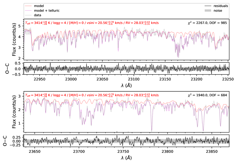
Figure 2: Best-fit forward model of a single frame for [HC2000] 244, orders 33 (top) and 32 (bottom). Plotted are the data (light gray lines), stellar model (red lines), and stellar model multiplied by the telluric spectrum (magenta lines). The bottom plot under each order shows the residuals (black lines) and the uncertainty in the flux (gray shaded regions). Best-fit parameters are listed in the top right corners, with $\log g$ and metallicity ([M/H]) fixed at 4 and 0, respectively. The residuals are dominated by fringing.

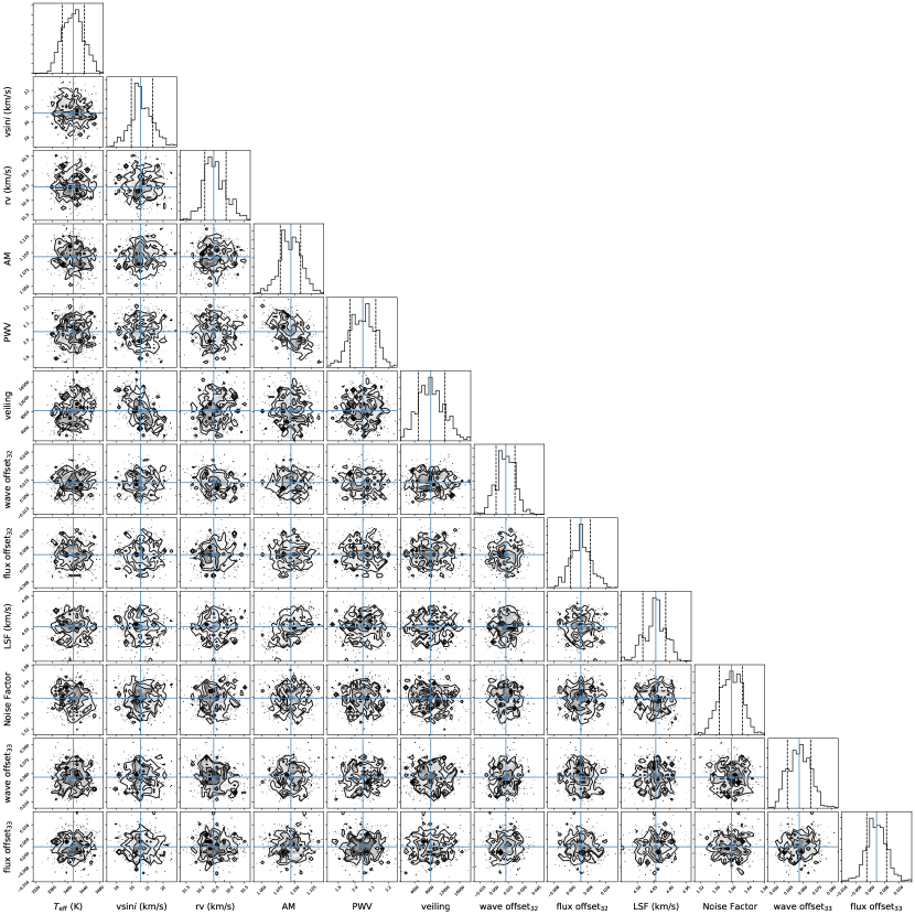
Figure 3: Corner plot of a single frame for [HC2000] 244. This corner plot corresponds to the fit in Figure 2. The subscripts in the parameter labels refer to the orders. The solid line shows the median of each distribution, and the dotted lines show the 16th and 84th percentiles.

Many of our sources converged to relatively high veiling parameters (i.e., $r_{\lambda}>0.2$), and we note that temperature should be highly degenerate with veiling ratio due to the strong dependence of the fits on the CO bands, which could be weakened either by higher effective temperatures or higher veiling ratios. However, we do not have sufficient data to put constraints on the veiling parameter for each source, as that would required a 3-D extinction map of the ONC (e.g., Schlafly et al., 2015), and precise distances to individual sources. However, even with the Gaia satellite (Gaia Collaboration et al., 2016) the embedded nature of the ONC makes parallax measurements extremely difficult (Kim et al., 2019). Therefore, this study is focused on the kinematics of the ONC, however, a future study will investigate the $T_{\mathrm{eff}}$ (and mass) dependence of kinematics in the ONC core.

Our RV measurements are relatively robust to changes in stellar parameters, since they are strongly anchored to the CO bandheads and the absolute calibration of the telluric spectrum. To illustrate this, we fit [HC2000] 244 (the same source shown in Figure 2) using the same procedure outlined above and holding the $\log g$ constant from 0 to 6 in steps of 0.5 (the resolution of the model grid). Figure 4 (top) shows the RV variation due to different $\log g$ values. For $\log g$ values that differ by more than $\pm$1 dex from the nominal value RV variations are more than 1%, however, those are extremely large variations in $\log g$ that are inconsistent with the youth of these targets. For RV values within $\pm$0.5 dex, the variation is less than 0.5%. To be conservative, we chose to add this systematic uncertainty to our combined measurement uncertainty across all frames for each single object.

We performed a similar test to the one above, this time holding temperature constant. Figure 4 (bottom) shows the RV variation due to different temperatures. Within a few hundred kelvin, the RV variation is less than 3%. However, within $\pm$100 K this value is less than 0.5%, which is within the systematic uncertainty found in the $\log g$ variation. Therefore, no additional systematic is required since the $\pm$0.5% systematic accounts for both the $\log g$ and $T_{\mathrm{eff}}$ variations. In summary, our reported uncertainties are the summed quadrature of our measurement uncertainty from the MCMC fits, the 0.058 km s^-1 systematic uncertainty between calibration frames, and the 0.5% variation found from differing $\log g$ and $T_{\mathrm{eff}}$.

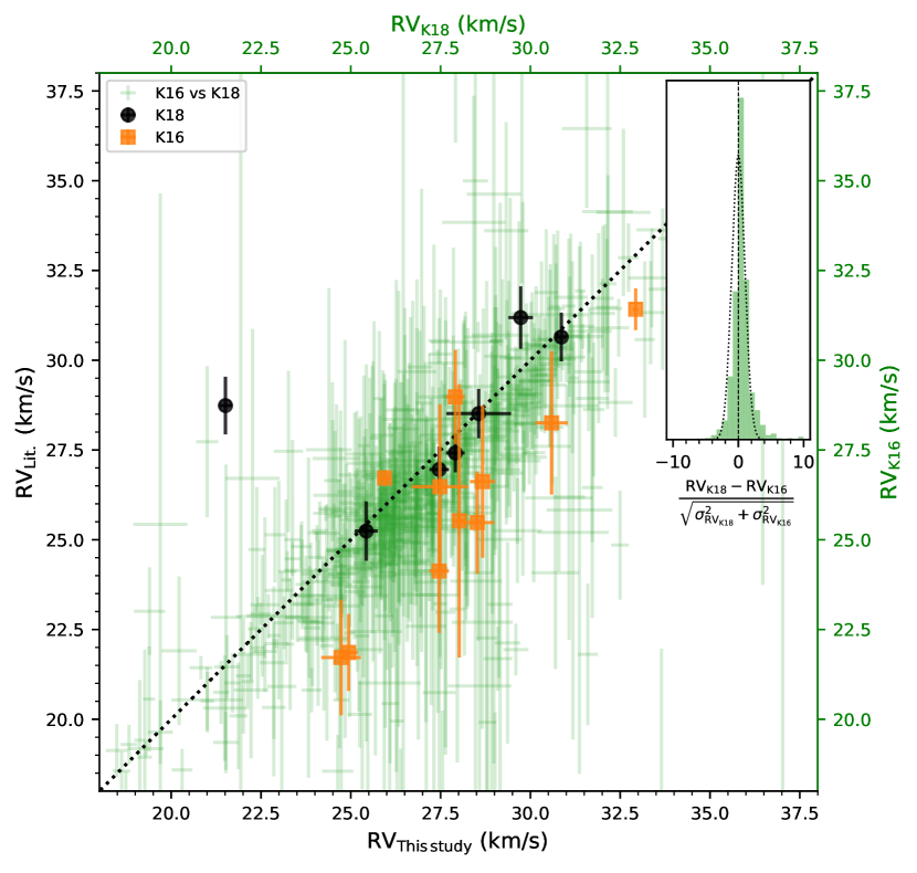
Figure 5: RV comparison between NIRSPEC RVs from this study and APOGEE RVs from K18 (black circles) and optical RVs from Kounkel et al. (2016, orange squares). K16 versus K18 are shown with translucent green markers (662 sources). The black dotted line indicates where RV measurements are equal. The large outlier, [HC2000] 546, is a potential RV variable binary. The inset plot shows the distribution of $(\mathrm{RV}_{\mathrm{K18}}-\mathrm{RV}_{\mathrm{K16}})/\sqrt{\sigma_{\mathrm{RV}_{\mathrm{K18}}}^{2}+\sigma_{\mathrm{RV}_{\mathrm{K16}}}^{2}}$ (green markers), which has $\mu=0.58$ km s^-1 and $\sigma=1.83$ km s^-1. This indicates that the K16 RVs are, on average, smaller than the K18 APOGEE RVs, and that the uncertainties in at least one of the surveys are underestimated. The inset plot shows a normal distribution with $\mu=0$ and $\sigma=1$ for comparison (dotted line).

Lastly, we compare our derived RVs to those from APOGEE using the results of K18, and Tobin et al. (2009), using the reanalyzed RVs from Kounkel et al. (2016, hereafter K16). Figure 5 shows the results of our RV comparison. In total, there were 11 matches between our NIRSPEC targets and the T09/K16 sample, and 7 matches to APOGEE (using a 0.5″crossmatch radius). Our results are consistent with the K18 APOGEE results with only 2 exceptions differentiating by more than 1-$\sigma$ of their combined uncertainty, possibly the result of spectroscopic binaries, 2MASS J05352104$-$0523490 and 2MASS J05351498$-$0521598. In comparison to optical RVs from T09/K16, our measured RVs are generally smaller than those measured from optical data, by $\sim$1.8 km s^-1 on average. We also compared K16 to K18 RVs, again using a 0.5″crossmatch radius, finding 586 sources in common (Figure 5, green pluses). The distribution of the uncertainty weighted difference between these two measurements, $(\mathrm{RV}_{\mathrm{K18}}-\mathrm{RV}_{\mathrm{K16}})/\sqrt{\sigma_{\mathrm{RV}_{\mathrm{K18}}}^{2}+\sigma_{\mathrm{RV}_{\mathrm{K16}}}^{2}}$, has a mean value of $\mu=0.58$ km s¹ and a standard deviation of $\sigma=1.83$ km s¹. This is consistent with the K16 values being, on average, smaller than the K18 APOGEE RVs. The width of the distribution also indicates that one, or both, of the uncertainties are underestimated. In general, RVs derived from NIR data versus optical are likely to suffer from fewer systematics in this highly embedded region.

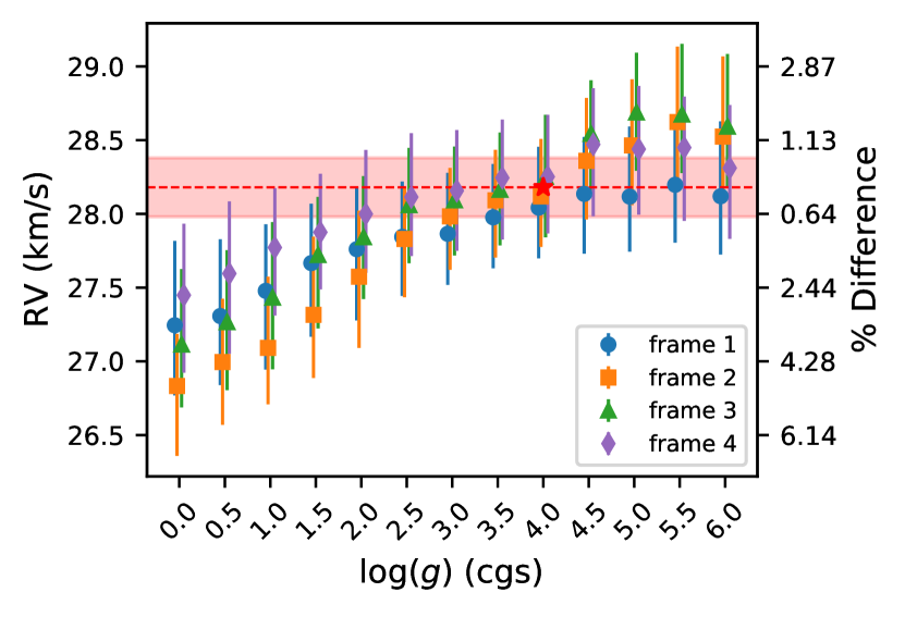
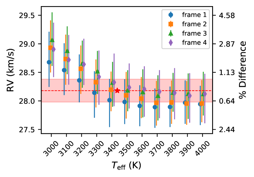
Figure 4: Best-fit RVs for [HC2000] 244 while keeping $\log g$ (top) and temperature (bottom) constant. Each marker shows one of the four frames. Top: The RV variation within $\log g\pm 0.5$ dex of our adopted values (28.18 km s^-1 and $\log g=4$; red star and dashed line, uncertainties shown with the filled area) is less than a 1%. Even at much lower/higher gravities the RV variation is not more than a few percent. At the age of the ONC, the expected surface gravity values are $\log g\sim 3$–4. Bottom: The RV variation within a few hundred kelvin of our adopted values (28.18 km s^-1 and 3436 K; red star and dashed line, uncertainties shown with the filled area) is less than a few percent.

Table 3: NIRSPEC Forward-Modeling Results

[HC2000]	ID	$\alpha_{J2000}$	$\delta_{J2000}$	$\overline{RV}$	$\mu_{\alpha\cos\delta}$	$\mu_{\delta}$	$T_{\mathrm{eff}}$	$v\sin{i}$	Veiling	Note
		(deg)	(deg)	(km s-1)	(mas yr-1)	(mas yr-1)	(K)	(km s-1)	$\left(\dfrac{F_{\mathrm{O33},\mathrm{cont}}}{F_{\mathrm{O33},\ast}}\right)$
135	$\cdots$	$83.80950000$	$-5.40686111$	$28.56\pm 0.91$	$\cdots$	$\cdots$	$3610\pm 300$	$49.33\pm 2.26$	0.24
188	559	$83.83175000$	$-5.39925000$	$29.74\pm 0.27$	$0.41\pm 0.52$	$-0.83\pm 0.18$	$3475\pm 73$	$6.90\pm 1.72$	0.01
202	615	$83.81666667$	$-5.39805556$	$25.69\pm 0.75$	$2.80\pm 0.06$	$-1.56\pm 0.08$	$3393\pm 204$	$42.27\pm 2.95$	0.75	E1
204	$\cdots$	$83.84087500$	$-5.39830556$	$24.73\pm 0.55$	$\cdots$	$\cdots$	$3712\pm 50$	$48.16\pm 2.56$	0.28
215	$\cdots$	$83.80116667$	$-5.39669444$	$27.91\pm 0.27$	$\cdots$	$\cdots$	$3641\pm 33$	$9.03\pm 1.41$	0.20
217	$\cdots$	$83.83770833$	$-5.39694444$	$29.73\pm 0.35$	$\cdots$	$\cdots$	$3614\pm 33$	$47.35\pm 0.89$	0.23	V
219	87	$83.81316667$	$-5.39630556$	$24.08\pm 0.48$	$1.87\pm 0.06$	$-0.65\pm 0.02$	$3486\pm 57$	$20.78\pm 1.40$	0.43
220	23	$83.81175000$	$-5.39625000$	$33.47\pm 0.23$	$-1.66\pm 0.40$	$0.08\pm 0.13$	$3484\pm 19$	$9.04\pm 0.30$	0.02
223	164	$83.81433333$	$-5.39597222$	$27.45\pm 0.23$	$1.10\pm 0.08$	$-0.68\pm 0.23$	$3359\pm 16$	$9.74\pm 0.69$	0.32
224	$\cdots$	$83.79475000$	$-5.39575000$	$25.94\pm 0.15$	$\cdots$	$\cdots$	$3859\pm 21$	$24.94\pm 0.58$	0.00
228	$\cdots$	$83.80250000$	$-5.39561111$	$27.46\pm 0.27$	$\cdots$	$\cdots$	$3782\pm 30$	$40.37\pm 0.78$	0.46
229	536	$83.83904167$	$-5.39594444$	$28.30\pm 0.21$	$0.12\pm 0.14$	$0.67\pm 0.27$	$3613\pm 79$	$12.19\pm 1.21$	0.15
240	$\cdots$	$83.80604167$	$-5.39455556$	$27.11\pm 0.44$	$\cdots$	$\cdots$	$3640\pm 65$	$14.15\pm 1.28$	3.89
244	180	$83.82108333$	$-5.39438889$	$28.18\pm 0.11$	$-0.02\pm 0.15$	$0.83\pm 0.40$	$3436\pm 17$	$21.29\pm 0.83$	0.04
245	$\cdots$	$83.81229167$	$-5.39425000$	$31.05\pm 0.21$	$\cdots$	$\cdots$	$3869\pm 18$	$17.03\pm 0.35$	0.00
248	200	$83.81566667$	$-5.39400000$	$26.56\pm 0.78$	$1.81\pm 0.43$	$-2.83\pm 0.20$	$3438\pm 48$	$39.39\pm 3.82$	0.35	E2
250	197	$83.81625000$	$-5.39388889$	$29.93\pm 0.46$	$1.70\pm 0.40$	$-3.85\pm 1.18$	$2975\pm 91$	$15.90\pm 1.86$	0.39	E2
253	$\cdots$	$83.82587500$	$-5.39330556$	$28.67\pm 0.36$	$\cdots$	$\cdots$	$4000\pm 117$	$6.21\pm 1.48$	2.66
258	521	$83.81000000$	$-5.39269444$	$28.02\pm 0.19$	$-0.11\pm 0.23$	$-1.65\pm 0.03$	$3568\pm 41$	$7.71\pm 1.03$	0.82
259	$\cdots$	$83.82112500$	$-5.39277778$	$27.53\pm 0.08$	$\cdots$	$\cdots$	$3501\pm 44$	$32.49\pm 1.95$	0.54
261	206	$83.81408333$	$-5.39261111$	$26.39\pm 0.20$	$-0.72\pm 0.24$	$0.87\pm 0.12$	$3374\pm 14$	$1.49\pm 0.31$	0.00
275	65	$83.81220833$	$-5.39141667$	$30.88\pm 0.01$	$-1.18\pm 0.14$	$1.19\pm 0.06$	$3860\pm 17$	$17.59\pm 0.30$	0.00
277A	530	$83.83525000$	$-5.39158333$	$25.88\pm 0.36$	$-0.81\pm 0.12$	$0.14\pm 0.06$	$3444\pm 51$	$12.90\pm 2.65$	0.36	B
282	44	$83.82866667$	$-5.39136111$	$26.96\pm 0.28$	$-0.85\pm 0.24$	$1.35\pm 0.03$	$3394\pm 22$	$5.59\pm 1.05$	1.06
288	71	$83.82966667$	$-5.39086111$	$26.61\pm 0.17$	$-0.42\pm 0.04$	$-0.52\pm 0.41$	$3666\pm 54$	$18.20\pm 0.53$	0.25
291	211	$83.81600000$	$-5.39044444$	$29.06\pm 0.22$	$1.10\pm 0.45$	$-1.63\pm 0.07$	$3181\pm 33$	$15.83\pm 0.72$	0.42	B
295	$\cdots$	$83.82320833$	$-5.39025000$	$21.85\pm 0.93$	$\cdots$	$\cdots$	$3662\pm 305$	$22.69\pm 7.18$	0.76
302	221	$83.81133333$	$-5.38969444$	$29.24\pm 0.11$	$-0.24\pm 0.40$	$0.71\pm 0.13$	$3541\pm 21$	$13.73\pm 1.12$	0.48
306A	$\cdots$	$83.81600000$	$-5.38958333$	$29.12\pm 0.50$	$\cdots$	$\cdots$	$4201\pm 229$	$25.92\pm 1.36$	1.12	B
306B	$\cdots$	$83.81600000$	$-5.38958333$	$21.15\pm 0.54$	$\cdots$	$\cdots$	$3473\pm 35$	$40.15\pm 2.53$	0.64	B
313	198	$83.82279167$	$-5.38919444$	$26.35\pm 0.19$	$1.07\pm 0.86$	$3.21\pm 0.20$	$4206\pm 235$	$10.04\pm 0.93$	0.64	E2
322	$\cdots$	$83.81787500$	$-5.38794444$	$24.90\pm 0.27$	$\cdots$	$\cdots$	$3414\pm 18$	$37.47\pm 0.92$	0.07
324	226	$83.81183333$	$-5.38777778$	$30.77\pm 0.34$	$0.70\pm 0.55$	$-1.87\pm 0.04$	$3449\pm 36$	$5.12\pm 1.21$	0.01
331	121	$83.82604167$	$-5.38769444$	$31.83\pm 0.69$	$1.26\pm 0.24$	$1.03\pm 0.04$	$4034\pm 452$	$18.92\pm 1.17$	0.64
332A	183	$83.82425000$	$-5.38766667$	$25.43\pm 0.32$	$-1.61\pm 0.17$	$0.60\pm 0.38$	$4012\pm 37$	$16.48\pm 0.43$	0.01	BC
370	227	$83.81616667$	$-5.38388889$	$31.24\pm 0.17$	$0.01\pm 0.74$	$-0.46\pm 0.09$	$3802\pm 45$	$14.43\pm 0.34$	0.66
375	560	$83.82075000$	$-5.38361111$	$33.19\pm 0.45$	$0.78\pm 0.13$	$1.15\pm 0.04$	$4225\pm 244$	$26.95\pm 0.70$	0.41
386	$\cdots$	$83.81362500$	$-5.38241667$	$27.44\pm 0.18$	$\cdots$	$\cdots$	$3673\pm 13$	$11.20\pm 0.10$	0.11
388	532	$83.82316667$	$-5.38244444$	$30.59\pm 0.46$	$0.65\pm 0.23$	$0.35\pm 0.04$	$4279\pm 142$	$17.83\pm 1.46$	0.52
389	$\cdots$	$83.81516667$	$-5.38233333$	$30.86\pm 0.15$	$\cdots$	$\cdots$	$3566\pm 34$	$26.89\pm 0.46$	0.68
408	143	$83.83008333$	$-5.38075000$	$23.52\pm 0.94$	$-1.51\pm 0.71$	$-1.07\pm 0.10$	$3660\pm 105$	$50.79\pm 1.85$	0.02
410	62	$83.82133333$	$-5.38058333$	$21.42\pm 1.91$	$-0.85\pm 0.29$	$0.32\pm 0.12$	$3910\pm 94$	$57.77\pm 2.25$	0.03
412	151	$83.81808333$	$-5.38030556$	$32.93\pm 0.32$	$1.21\pm 0.20$	$0.51\pm 0.27$	$3563\pm 28$	$31.96\pm 1.61$	0.80
413	35	$83.81454167$	$-5.38016667$	$25.51\pm 0.41$	$-0.43\pm 0.04$	$-0.27\pm 0.74$	$3643\pm 44$	$28.79\pm 0.55$	0.05
420	154	$83.81600000$	$-5.37941667$	$25.91\pm 0.24$	$-0.38\pm 0.31$	$-1.82\pm 0.25$	$3510\pm 35$	$24.16\pm 0.67$	0.00
425	$\cdots$	$83.82479167$	$-5.37930556$	$24.94\pm 0.25$	$\cdots$	$\cdots$	$3576\pm 22$	$21.83\pm 0.32$	0.00
431	700	$83.81216667$	$-5.37752778$	$33.49\pm 0.31$	$1.68\pm 0.60$	$0.05\pm 0.94$	$3603\pm 22$	$18.80\pm 0.97$	0.65
436	$\cdots$	$83.82658333$	$-5.37708333$	$32.93\pm 0.08$	$\cdots$	$\cdots$	$3658\pm 347$	$16.30\pm 0.90$	0.11
440	$\cdots$	$83.82233333$	$-5.37661111$	$28.52\pm 0.48$	$\cdots$	$\cdots$	$3715\pm 88$	$23.57\pm 1.07$	1.37
450	$\cdots$	$83.82087500$	$-5.37586111$	$26.23\pm 0.24$	$\cdots$	$\cdots$	$3674\pm 54$	$12.14\pm 0.74$	0.02
504	64	$83.81395833$	$-5.37100000$	$27.48\pm 0.78$	$-0.29\pm 0.15$	$-0.32\pm 0.02$	$3969\pm 295$	$30.65\pm 1.86$	3.79
522A	110	$83.81787500$	$-5.36955556$	$24.75\pm 0.47$	$0.03\pm 0.10$	$-1.97\pm 0.14$	$3441\pm 24$	$33.48\pm 1.98$	0.31	B
522B	642	$83.81787500$	$-5.36955556$	$24.54\pm 0.28$	$-0.69\pm 0.11$	$0.48\pm 0.33$	$3170\pm 39$	$21.94\pm 1.20$	0.80	B
546	567	$83.81250000$	$-5.36666667$	$21.51\pm 0.18$	$2.25\pm 0.09$	$0.96\pm 0.11$	$3793\pm 56$	$15.32\pm 1.18$	0.27	V
703	137	$83.80750000$	$-5.36863889$	$33.39\pm 0.06$	$-1.51\pm 0.90$	$-1.03\pm 0.52$	$3584\pm 27$	$9.14\pm 0.41$	1.24
713	$\cdots$	$83.82795833$	$-5.38247222$	$22.95\pm 0.31$	$\cdots$	$\cdots$	$4988\pm 192$	$6.75\pm 1.54$	1.60

4 APOGEE Reanalysis

It is useful to assess the fidelity of the parameters derived in our pipeline by applying it to an independent dataset. We chose to apply our pipeline to APOGEE $H$-band data. These data have independent measurements of $T_{\mathrm{eff}}$, $\log g$, and RVs of ONC sources from K18. We chose to do a subset of the entire K18 catalog, selecting objects within 4′ of the ONC CoM (172 sources). We used a similar version of our aforementioned pipeline (see Section 3.1), with the flux for each chip modeled using equation (2). The LSF was modeled as a sum of Gauss-Hermite functions (Nidever et al., 2015), obtained using the apogee code (Bovy, 2016). It should be noted that our model choice of PHOENIX-ACES-AGSS-COND-2011 (Husser et al., 2013) is the same as that used in K18.

We fit all three chips simultaneously (A: 1.647–1.696 $\mu$m, B: 1.585–1.644 $\mu$m, and C: 1.514–1.581 $\mu$m), allowing each chip to have separate nuisance parameters (e.g., $C0_{\mathrm{flux,A}}$ and $C1_{\mathrm{flux,A}}$ for chip A, $C0_{\mathrm{flux,B}}$ and $C1_{\mathrm{flux,B}}$ for chip B), similar to our simultaneous modeling of separate NIRSPEC orders. In general, the APOGEE sources tend to be much brighter than our NIRSPEC sources; however, the median $H$-band veiling ratio for APOGEE sources is 0.58, and these sources are more susceptible to confusion due to the size of the fiber (2″ diameter; Majewski et al., 2017). The results of our fits are listed in Table 5, including measured veiling ratios and noting sources where a nearby companion could confuse results. We show comparisons of our derived $T_{\mathrm{eff}}$ and RVs to those from K18 in Figure 7. Our derived temperatures are overall consistent with K18, although there is a small systematic shift from low to high temperatures. Our RVs are consistent with those from K18 ($\overline{\Delta\mathrm{RV}}=0.23\pm 0.43$ km s^-1), with a number of sources having measured RVs where K18 only provided upper limits. In total, we provide RV measurements for 87 sources that previously had no measurement in K18. We note that although these sources have no definitive measurement in K18, many of these sources have RV measurements from the SDSS/APOGEE processing pipeline (Nidever et al., 2015). However, K18 mention that these estimates tend to be unreliable for sources with $T_{\mathrm{eff}}<3000$ K, and potentially also for YSOs, where veiling must be accounted for.

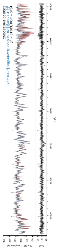
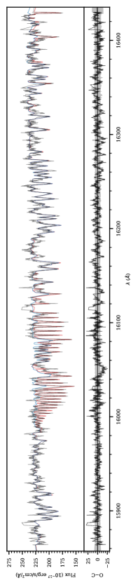
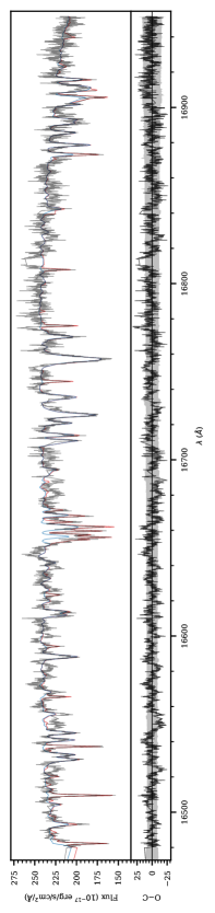
Figure 6: Example fit to APOGEE data for all three chips. Raw APOGEE data are shown in gray, the best-fit stellar model is shown in blue (parameters given in the upper right hand corner), and the best-fit stellar model convolved with the best-fit telluric model is shown in red. Residuals are shown in the lower plot (black line), along with the flux uncertainty (gray region).

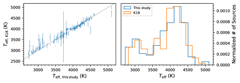
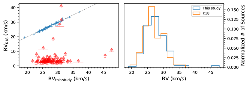
Figure 7: Comparison between our derived parameters using APOGEE spectra and those derived in K18 (168 sources). Black dotted lines indicate where agreement is one-to-one. Top: $T_{\mathrm{eff}}$ comparison. There is a slight offset, with our derived $T_{\mathrm{eff}}$ being slightly lower than K18 for $T_{\mathrm{eff}}<3600$, and slightly higher than K18 for $T_{\mathrm{eff}}>3600$. Bottom: RV comparison. Red arrows represent lower limits as reported by K18, while we provide measurements with errorbars.

5 The Kinematic Structure of the ONC Core

Three-dimensional kinematic studies of the ONC core have been primarily focused on the Trapezium Stars, as they are the brightest objects in the highly embedded region (e.g., Olivares et al., 2013). From Figure 1 it can be seen that very few previous studies have obtained RVs for sources within the direct vicinity of the Trapezium stars. Here, we analyze the 3-D kinematics of sources that make up the “core” of the ONC.

5.1 Tangential Velocities

Our measurements provide velocities along the line of sight; however, to measure 3-D velocities we require tangential motions. A number of studies have measured the PMs of sources within the ONC (e.g., Parenago, 1954; Jones & Walker, 1988; van Altena et al., 1988; Gómez et al., 2005; Dzib et al., 2017; Kuhn et al., 2019; Kim et al., 2019; Platais et al., 2020). The two most recent catalogs produced by Kim et al. (2019) and Platais et al. (2020) both use imaging data from the Hubble Space Telescope (HST). We chose to adopt the values from Kim et al. (2019) as their combination of HST imaging with data from the Keck Near Infrared Camera 2 (NIRC2; PI: K. Matthews) provide a baseline of $\sim$20 years. Additionally, the uncertainties published by Platais et al. (2020) tend to be very small, and are possibly underestimated due to the fact that they were unable to determine systematic uncertainties. This likely explains their much smaller errors versus Kim et al. (2019), even though a shorter time baseline of $\sim$11 years was used.

The Kim et al. (2019) catalog includes PM measurements for 701 sources with typical uncertainties $\lesssim$1 mas yr^-1. However, to convert PMs into tangential velocities we require a distance, or distance distribution, to the ONC. a number of studies have investigated the distance to the ONC using Very-long-baseline interferometry (VLBI; Menten et al., 2007; Sandstrom et al., 2007; Kounkel et al., 2017), and, more recently, Gaia Data Release 2 (Gaia Collaboration et al., 2018; Kounkel et al., 2018; Großschedl et al., 2018; Kuhn et al., 2019). The majority of these measurements are consistent with an average distance to the ONC of $\sim$390 pc. For our study, we adopted the VLBI trigonometric distance of $388\pm 5$ pc from Kounkel et al. (2017), which is consistent with Kounkel et al. (2018, $389\pm 3$ pc, Gaia DR2;), Kuhn et al. (2019, $403^{+7}_{-6}$ pc, Gaia DR2;), Großschedl et al. (2018, $397\pm 16$ pc, Gaia DR2;), and ($389^{+24}_{-21}$ pc, VLBI; Sandstrom et al., 2007)

Using the above distance estimate, we converted PMs to tangential velocities, combining errors in PMs and the distance to the ONC using standard error propagation. The combined sample with all three components of motion totaled 135 sources. Figure 8 shows a map of the ONC with vectors displaying the PM of sources in our sample and colors representing the measured RVs. All three components of motion for our subsample are shown in Figure 9. These velocities were used to investigate the 3-D kinematics of the ONC core region. There are a number of kinematic outliers, both in tangential velocity space (as discussed in Kim et al. 2019), and in radial velocity space, which will be discussed in Section 5.3.

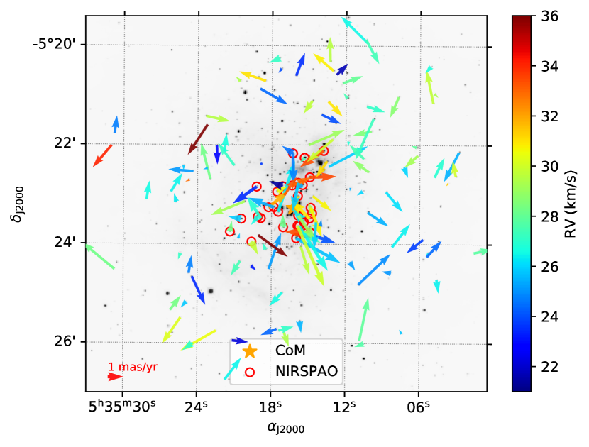
Figure 8: Diagram of PMs and line of sight velocities for sources within a $4\arcmin\times 4\arcmin$ window centered on the core of the ONC. The background image is a CTIO/Blanco ISPI $K_{s}$-band image from Robberto et al. (2010). Sources with NIRSPAO RVs are denoted with red circles, while the remaining sources have RVs measured from APOGEE data. The CoM for the ONC is indicated by the orange star.

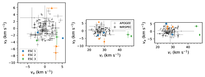
Figure 9: Plots of each velocity component with respect to one another. All axes have equal scaling. Shown are APOGEE measurements (gray points), NIRSPEC measurements (black points), and kinematic outliers (see Section 5.3) from escape groups 1 (blue squares), 2 (orange triangles), and 3 (green diamonds).

5.2 Intrinsic Velocity Dispersion Calculation

To determine velocity dispersion, we utilized a similar Bayesian framework to Kim et al. (2019), where each $i$-th kinematic measurement is parameterized as $v_{(\alpha,\delta,r)_{i}}\pm\epsilon_{{(\alpha,\delta,r)}_{i}}$. We assume each kinematic measurement is drawn from a multivariate Gaussian distribution with mean values of $\bar{v}_{\alpha}$, $\bar{v}_{\delta}$, and $\bar{v}_{r}$, and standard deviations of $\sqrt{\sigma_{v_{(\alpha,\delta,r)}}^{2}+\epsilon_{(\alpha,\delta,r)_{i}}^{2}}$, where $\sigma_{v_{\alpha}}$, $\sigma_{v_{\delta}}$, and $\sigma_{v_{r}}$ are the intrinsic velocity dispersions (IVDs). The log-likelihood for the three dimensional kinematics of the $i$-th object is given by

$$\ln L_{i}=-\frac{1}{2}\left[\ln(|\boldsymbol{\Sigma}_{i}|)+(\boldsymbol{v}_{i}-\boldsymbol{\mu})^{{{\!\mathsf{T}}}}\boldsymbol{\Sigma}^{-1}_{i}(\boldsymbol{v}_{i}-\boldsymbol{\mu})+3\ln(2\pi)\right],$$ (4)

where the input kinematic measurement vector for the $i$-th object $\boldsymbol{v}_{i}$ is defined as

$$\boldsymbol{v}_{i}=\begin{bmatrix}v_{\alpha_{i}}\\ v_{\delta_{i}}\\ v_{r_{i}}\end{bmatrix},$$ (5)

while the vectors for the mean velocities and dispersions are defined as

$$\boldsymbol{\mu}=\begin{bmatrix}\bar{v}_{\alpha}\\ \bar{v}_{\delta}\\ \bar{v}_{r}\end{bmatrix},\hskip 35.0pt \boldsymbol{\sigma}=\begin{bmatrix}\sigma_{v_{\alpha}}\\ \sigma_{v_{\delta}}\\ \sigma_{v_{r}}\end{bmatrix},$$ (6)

and the covariance matrix $\boldsymbol{\Sigma}_{i}$ for the $i$-th object is defined as

$$\boldsymbol{\Sigma}_{i}=\begin{bmatrix}\sigma_{v_{\alpha}}^{2}+\epsilon_{\alpha_{i}}^{2}&\begin{split}\rho_{1}(\sigma_{v_{\alpha}}&\sigma_{v_{\delta}}+\\ &\epsilon_{\alpha_{i}}\epsilon_{\delta_{i}})\end{split}&\begin{split}\rho_{2}(\sigma_{v_{\alpha}}&\sigma_{v_{r}}+\\ &\epsilon_{\alpha_{i}}\epsilon_{r_{i}})\end{split}\\ \begin{split}\rho_{1}(\sigma_{v_{\alpha}}&\sigma_{v_{\delta}}+\\ &\epsilon_{\alpha_{i}}\epsilon_{\delta_{i}})\end{split}&\sigma_{v_{\delta}}^{2}+\epsilon_{\delta_{i}}^{2}&\begin{split}\rho_{3}(\sigma_{v_{\delta}}&\sigma_{v_{r}}+\\ &\epsilon_{\delta_{i}}\epsilon_{r_{i}})\end{split}\\ \begin{split}\rho_{2}(\sigma_{v_{\alpha}}&\sigma_{v_{r}}+\\ &\epsilon_{\alpha_{i}}\epsilon_{r_{i}})\end{split}&\begin{split}\rho_{3}(\sigma_{v_{\delta}}&\sigma_{v_{r}}+\\ &\epsilon_{\delta_{i}}\epsilon_{r_{i}})\end{split}&\sigma_{v_{r}}^{2}+\epsilon_{r_{i}}^{2}\end{bmatrix}.$$ (7)

The correlation coefficients are given by $\rho_{1,2,3}$, and should be 0 if the covariance is completely uncorrelated. Using Bayes’s theorem, for a set of $N$ measurements $\boldsymbol{D}\equiv\{\boldsymbol{v}_{i},\boldsymbol{\epsilon}_{i}\}^{N}_{i=1}$, the log of the posterior probability is given as

$$\ln P(\boldsymbol{\mu},\boldsymbol{\sigma}|\boldsymbol{D})\varpropto\sum_{i}^{N}\left[\ln L_{i}(\boldsymbol{v}_{i},\boldsymbol{\epsilon}_{i}|\boldsymbol{\mu},\boldsymbol{\sigma})+\ln p(\boldsymbol{\mu},\boldsymbol{\sigma})\right],$$ (8)

where $p(\boldsymbol{\mu},\boldsymbol{\sigma})\equiv p(\boldsymbol{\mu})p(\boldsymbol{\sigma})$ is the prior on the means and dispersions. Similar to Kim et al. (2019), we adopted a flat prior on the mean vector, $\boldsymbol{\mu}$, and a Jeffreys prior on the dispersion vector, $p(\boldsymbol{\sigma})\varpropto\boldsymbol{\sigma}^{-1}$. To determine best-fit parameters for $\bar{v}_{\alpha}$, $\bar{v}_{\delta}$, $\bar{v}_{r}$, $\sigma_{v_{\alpha}}$, $\sigma_{v_{\delta}}$, $\sigma_{v_{r}}$, $\rho_{1}$, $\rho_{2}$, and $\rho_{3}$, we utilized the Monte Carlo Markov Chain (MCMC) affine-invariant ensemble sampler emcee (Foreman-Mackey et al., 2013).

5.3 Kinematic Outliers

Previous studies have identified subpopulations within the ONC with kinematics consistent with high-velocity escaping stars (e.g., Kim et al., 2019; Kuhn et al., 2019; Platais et al., 2020). Kim et al. (2019) and Kuhn et al. (2019) used outliers from an expected normal distribution to determine kinematic outliers. Kim et al. (2019) also used the ONCs 2-D mean-square escape velocity ($\approx$3.1 mas yr^-1, or 6.1 km s^-1 at a distance of 414 pc) to identify potential escaping sources. It should be noted that Kim et al. (2019) used a distance of $414\pm 7$ pc from Menten et al. (2007), whereas our adopted value of $388\pm 5$ pc would give a mean-square escape velocity of 5.7 km s^-1. In practice this should not alter results since outliers are computed from the bulk properties of the cluster, and our smaller distance would equally impact all tangential velocities the same.

To determine high-probability escaping or evaporating sources, we identified sources whose velocities deviate from the Gaussian velocity distribution model (see Section 5.2). We used a methodology similar to Kim et al. (2019) and Kuhn et al. (2019) plotting sources on $Q$-$Q$ plots, where data quantiles ($Q_{\mathrm{data}}$) are plotted against theoretical quantiles ($Q_{\mathrm{theo}}$) corresponding to a Gaussian distribution. These two quantiles are defined as

$$Q_{\mathrm{data},i}=\frac{v_{{(\alpha,\delta,r)}_{i}}-\bar{v}_{(\alpha,\delta,r)}}{\sqrt{\sigma_{(\alpha,\delta,r)}^{2}+\epsilon_{{(\alpha,\delta,r)}_{i}}^{2}}},$$ (9)

$$Q_{\mathrm{theo},i}=\sqrt{2}\ \mathrm{erf}^{-1}\left(\frac{2(r_{i}-0.5)}{n}-1\right),$$ (10)

where erf^-1 is the inverse of the error function, $r_{i}$ is the rank of the $i$-th measurement, and $n$ is the number of measurements.

The means and IVDs are computed using the method outlined in Section 5.2. Figure 10 shows the quantiles for all sources (top plot), quantiles after removing outliers in RV space (middle plot), and quantiles after removing large outliers in RV and tangential kinematic space (bottom plot). In each plot, the gray band indicates the 95% confidence interval from bootstrapping. Kim et al. (2019) identified two separate groups of kinematic outliers, sources with highly significant deviations within the $Q$-$Q$ plot ($Q_{\mathrm{data},X}\geq\pm$3; escape group 1), and sources with low-significance escape velocities defined from the angular escape speed (sources with $\mu_{\mathrm{tot}}>3.1$ mas yr^-1; escape group 2). We additionally identify sources with RVs that significantly deviate from the sample ($Q_{\mathrm{data},Z}\geq\pm$3), and label this escape group 3 (see Figures 9 and 10). Kim et al. (2019) and Kuhn et al. (2019) estimated the escape speed for the ONC to be $\approx 6.1$ km s^-1 using the virial theorem, and all of the outliers in escape groups 1 and 3 have velocities in excess of this speed. However, it should be noted that velocity outliers in RV space could be potential binaries rather than escaping/evaporating sources.

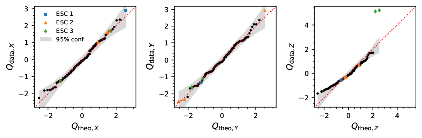
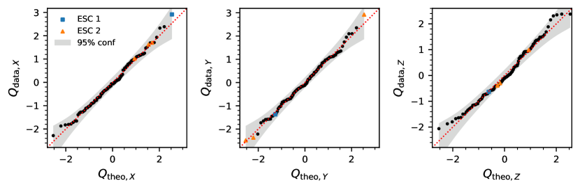
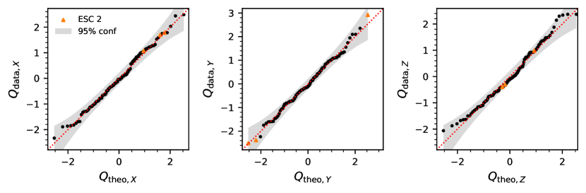
Figure 10: $Q$-$Q$ plots showing the normality of the three velocity components (from left to right: $v_{\alpha}$, $v_{\delta}$, and $v_{r}$). High velocity (blue squares) and low velocity (orange triangles) escaping sources identified by Kim et al. (2019) are indicated. Additionally, velocity outliers from this study are indicated with green diamonds. Top: Analysis including all sources. Middle: Analysis after removing the escape group 3 sources. Bottom: Analysis after removing all sources in escape groups 1 and 3.

Of the escaping stars identified in Kim et al. (2019), one of the sources in escape group 1 and three of the sources in escape group 2 were observed with NIRSPAO, and none were in our reanalyzed APOGEE subsample (identified in Table 3). This is not surprising as all of the sources in escape groups 1 and 2 are within 2.5′ of the ONC CoM (16 of 18 sources within 1′). The majority of sources in escape groups 1 and 2 tend to be fainter (14 of 18 sources with F139 mag $\gtrsim 12$), or have a nearby source within 2″. All of the sources in escape groups 1 and 2 have RVs that are consistent with the bulk RV distribution of the ONC. Conversely, none of the sources in escape group 3 (line of sight velocity outliers) are within escape groups 1 and 2, and both escape group 3 sources are APOGEE sources. This indicates that the high velocity components for these sources are primarily in either the tangential or line of sight direction, but not both.

5.4 Intrinsic Velocity Dispersions (IVDs)

Using the framework outlined in Section 5.2, we computed intrinsic velocity dispersions after removing all sources in escape groups 1 and 3. The values from our model were:

$$\bar{v}_{\alpha} =0.01\pm 0.16~{}\mathrm{km~{}s}^{-1},$$

$$\bar{v}_{\delta} =-0.09\pm 0.18~{}\mathrm{km~{}s}^{-1},$$

$$\bar{v}_{r} =27.45_{-0.22}^{+0.21}~{}\mathrm{km~{}s}^{-1},$$

$$\sigma_{v_{\alpha}} =1.64\pm 0.12~{}\mathrm{km~{}s}^{-1},$$

$$\sigma_{v_{\delta}} =2.03\pm 0.13~{}\mathrm{km~{}s}^{-1},$$

$$\sigma_{v_{r}} =2.56_{-0.17}^{+0.16}~{}\mathrm{km~{}s}^{-1},$$

$$\rho_{1} =0.06\pm 0.09,$$

$$\rho_{2} =-0.11\pm 0.09,$$

$$\rho_{3} =-0.05\pm 0.09.$$

The correlation coefficients are consistent with 0, indicating little to no correlation between velocity components.

Our computed velocity dispersions are roughly consistent with other studies in both the tangential (plane of the sky) direction: ($\sigma_{v_{\alpha}}$, $\sigma_{v_{\delta}}$) = ($1.63\pm 0.04$, $2.20\pm 0.06$) km s^-1 (K19); ($\sigma_{v_{\alpha}}$, $\sigma_{v_{\delta}}$) = ($1.85\pm 0.04$, $2.45\pm 0.06$) km s^-1 (Platais et al., 2020); and ($\sigma_{v_{\alpha}}$, $\sigma_{v_{\delta}}$) = ($1.79\pm 0.12$, $2.32\pm 0.10$) km s^-1 (Jones & Walker, 1988), and in the line of sight direction: $\sigma_{v_{r}}\approx 3.1$ km s^-1 (Fűrész et al., 2008); $\sigma_{v_{r}}\approx 2.1$–2.4 km s^-1 (Tobin et al., 2009); and $\sigma_{v_{r}}\approx 2.2$ km s^-1 (Da Rio et al., 2017). However, our derived value of $\sigma_{v_{r}}=2.56_{-0.17}^{+0.16}$ km s^-1 is slightly higher than the value measured in Tobin et al. (2009) and Da Rio et al. (2017). This is possibly due to our closer proximity to the ONC core than previous studies, or potentially the target selection of fainter, redder (lower-mass) sources. This may also indicate kinematic structure along the line of sight direction, similar to the velocity elongation seen in the north-south direction along the filament (e.g., Jones & Walker, 1988). It is also possible that this component potentially suffers from the impact of unresolved binaries, which we evaluate in the next section.

We identified one new binary candidate within our sample ([HC2000] 332A), along with six other targets being components of apparent doubles (candidate binaries). At least one source ([HC2000] 546) shows significant RV variability between APOGEE and NIRSPAO measurements, although no secondary component was detected in the AO imaging. There is only one epoch of APOGEE data and one epoch of NIRSPAO data for [HC2000] 546, therefore, it is not possible to determine the orbital parameters of this potential binary without additional observations. Two of our sources have multi-epoch NIRSPAO observations ([HC2000] 229 and [HC2000] 217), however, RVs computed at each epoch are consistent with one another within errors.

5.4.1 Unresolved Binarity

Radial velocities are instantaneous velocity measurements, in contrast to PM measurements which are taken over baselines of years. The effects of binary orbital motion therefore influence RV measurements, but are typically averaged out over the long time baselines of PM measurements. Consequently, it is important for us to quantify the potential effects that unresolved binaries may have on the line of sight velocity dispersion(s).

Raghavan et al. (2010) did an extensive multiplicity study of solar-type stars, both in the field and young sources determined from chromospheric activity. Their findings were that the overall field multiplicity of solar-type stars is $44\%\pm 4\%$, with the multiplicity fraction of younger sources being statistically equivalent $40\%\pm 3\%$. Additionally, Raghavan et al. (2010) also noted a declining trend in the multiplicity fraction with redder color (lower primary mass). Down to the M dwarf regime, the multiplicity fraction for the field is estimated to be $\sim$20%–25%, declining with lower primary mass (Fischer & Marcy, 1992; Clark et al., 2012; Ward-Duong et al., 2015; Bardalez Gagliuffi et al., 2019).

In the ONC, estimates of visual binaries range from $\sim$3%–30% (Köhler et al., 2006; Reipurth et al., 2007; Duchêne et al., 2018; De Furio et al., 2019; Jerabkova et al., 2019). Over the specific range investigated by Duchêne et al. (2018)—0.3–2 $M_{\sun}$ with companions within 10–60 au—they found the ONC binary fraction approximately 10% higher than the field population estimates from Raghavan et al. (2010) and Ward-Duong et al. (2015). Combined, this would place the binary fraction between 30%–50% for systems with primary masses between 0.1–1 $M_{\sun}$. These results are roughly consistent with modeling estimates (e.g., Kroupa et al., 1999; Kroupa, 2000; Kroupa et al., 2001).

With such a large potential binary fraction in the ONC, it is important quantify how orbital motion can affect our measured line of sight velocity dispersion. This is primarily important to determine whether the observed anisotropy between the line of sight component and the tangential components is explained with orbital motion, or if there is a true elongation along the line of sight velocities.

5.4.2 Simulating the Effect of Binaries

To determine the effects of unresolved binarity on the IVD, we performed a test similar to Da Rio et al. (2017) and Karnath et al. (2019). First, we generate a random intrinsic dispersion drawn from a uniform sample between 1–4 km s^-1. Next, we convolve this dispersion with the measurement error distribution. We use our observed measurement error distribution from the APOGEE+NIRSPEC dataset, and create an inverse cumulative distribution function which we randomly sample to build the error distribution. Lastly, we convolve this distribution with a velocity distribution from a set of synthetic binaries, and compare the final distribution to our observed distribution.

To generate our synthetic systems, we first generate a distribution of stars with masses between 0.1–1 $M_{\sun}$. We apply a binary fraction (discussed below) to our sample, and use the mass ratio distribution from Reggiani & Meyer (2013) to determine component masses within each system. Next, for binary systems, we apply the eccentricity distribution from Duchêne & Kraus (2013), and the period distribution from Raghavan et al. (2010).

For our simulations we generate 135 systems (the same number of sources in our 3-D kinematics sample). These synthetic systems are created using the velbin package (Cottaar & Hénault-Brunet, 2014; Foster et al., 2015). This sampling assumes random orbits with random orientations and provides a one-dimensional radial velocity distribution.

This distribution is then compared to our observed APOGEE+NIRSPEC RV distribution, requiring that the standard deviation of the synthetic distribution be within 2-$\sigma$ of the observed distribution’s standard deviation. An example of one randomly drawn distribution compared to our observed distribution is shown in Figure 11. The binary contribution to the resulting distribution is typically far less than the intrinsic dispersion and measurement error distribution, a result also noted by Da Rio et al. (2017).

We kept the first 10⁵ models that fit our similarity criteria stated above and generate a distribution of intrinsic velocity dispersions that passed the similarity criteria of our observed RV distribution. We performed this test for binary fractions of 0%, 25%, 50%, 75%, 100%. Figure 12 shows our simulation results compared to our IVD determined in Section 5.4. Figure 12 illustrates that our measured IVD is consistent with any level of binarity, however, for the line of sight component to be consistent with the tangential components, the ONC would need a binary fraction $\gtrsim$75%, which is inconsistent with observations and modeling results. Therefore, the larger measured $\sigma_{v_{r}}$ is likely due to formation/evolution rather than binary effects, and the apparent elongation in the line of sight component appears to be real rather than a systematic.

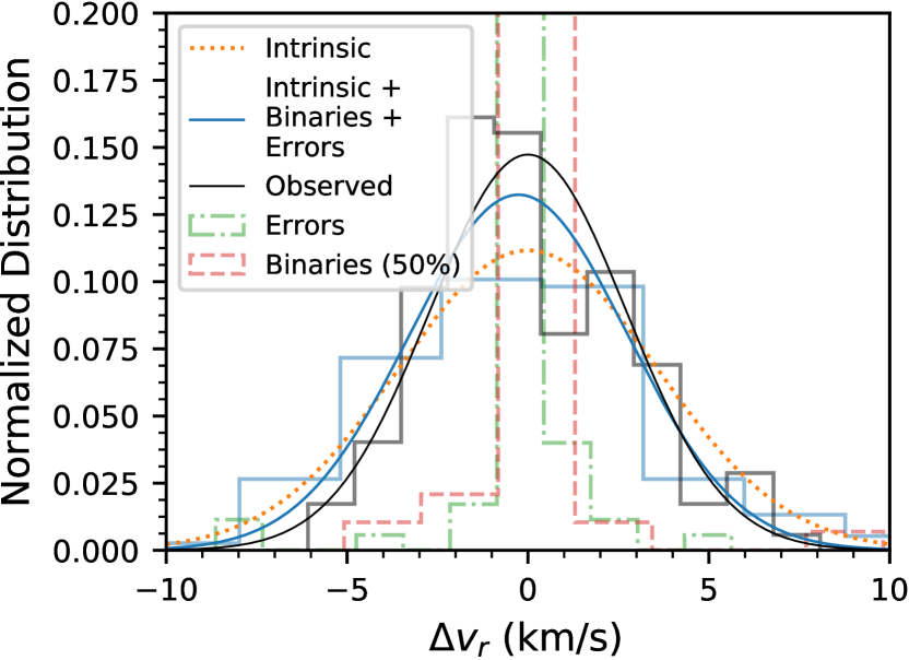
Figure 11: Example of a single model generated in our binary simulation. The gray distribution and black solid line indicate our observations. The orange dotted line shows the intrinsic IVD distribution, and the green dash-dotted and red dashed lines indicate the distributions of uncertainties and binaries, respectively. The blue line and distribution show the final distribution accounting for binaries and uncertainties, which is compared to observations. Binaries and measurement uncertainties work to widen the dispersion, making the observed velocity dispersion larger than the intrinsic velocity dispersion.

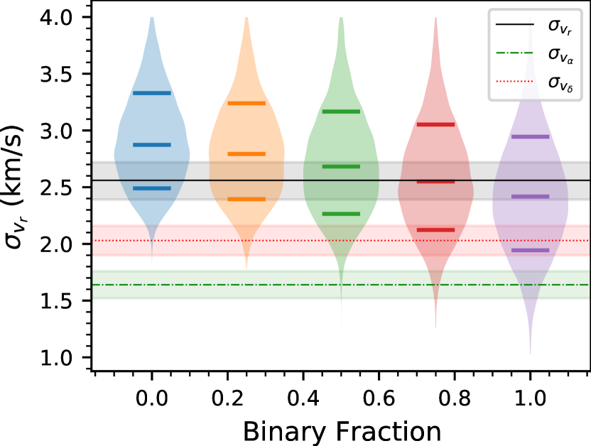
Figure 12: Violin plots showing the distributions of our binary simulations. Distributions are generated at binary fractions of 0%, 25%, 50%, 75%, and 100%, and lines within each distribution indicate 16th, 50th, and 84th percentiles. Our measured IVD (black line and gray 1-$\sigma$ confidence region) is consistent with a essentially all binary fractions. We also show our tangential IVD components in $\alpha$ (green dashed line and region) and $\delta$ (red dotted line and region), indicating that the binary fraction would need to be $\gtrsim$75% to bring the line of sight component within the range of the tangential components.

6 Discussion

6.1 Virial State of the ONC Core

A number of studies have examined if the ONC is virialzed (e.g., Jones & Walker, 1988; Da Rio et al., 2014, 2017; Kim et al., 2019; Kuhn et al., 2019). Da Rio et al. (2014) estimated a 1-D mean velocity dispersion of $\sigma_{v,\mathrm{1D}}\approx 1.73$ km s^-1 if the ONC is in virial equilibrium. To test for a virialized state, we adopt a methodology similar to Kim et al. (2019), computing the 1-D velocity dispersion as a function of radial distance outwards.

To balance the small numbers in our sample, we chose radial bins of size 1′. For each bin, we computed velocity dispersion using the methods outlined in Section 5.2. The values of $\sigma_{\alpha}$ and $\sigma_{\delta}$ where then used to compute the 1-D velocity dispersion, i.e., $\sigma_{v,\mathrm{1D}}^{2}=(\sigma_{v_{\alpha}}^{2}+\sigma_{v_{\delta}}^{2})/2$. Our computed velocity dispersions are listed in Table 4 and also plotted in Figure 13. We also show the 1-D velocity dispersion predicted for models of virial equilibrium using the estimated combined gas and stellar mass from Da Rio et al. (2014, solid line). We assigned a 30% mass uncertainty, similar to Kim et al. (2019), which are illustrated with dotted lines. It should be noted that the model from Da Rio et al. (2014) assumes a spherical potential; however, there is evidence that the potential is closer to an elongated spheroid (e.g., Hillenbrand & Hartmann, 1998; Carpenter, 2000; Kuhn et al., 2014; Kuznetsova et al., 2015; Megeath et al., 2016).

The 1-D velocity dispersion computed from proper motions is extremely consistent with the results of Kim et al. (2019), which is expected since our subsample originated from their catalog. The 1-D velocity dispersions favor a virialized state for the majority of the ONC. The radial distribution of $\sigma_{v_{r}}$ is similar to that from Da Rio et al. (2017, see Figure 12) for the ONC, although, they only show 1 bin from $R\sim 0$–0.4 pc. However, they also find a dispersion 1-$\sigma$ higher than the virial equilibrium model predicts. We also computed the one-dimensional velocity dispersion using all three velocity components $\sigma^{2}_{v,\mathrm{1D_{3D}}}=(\sigma^{2}_{v_{\alpha}}+\sigma^{2}_{v_{\delta}}+\sigma^{2}_{v_{r}})/3$, listed in Table 4. This measurement marginalizes over potential differences in a single velocity component. Figure 13 (bottom panel) shows that only the bin closest to the ONC core appears elevated from the virialized model, however, this method may wash out features in a single velocity component which deviate from a virialized state. These results add to the growing evidence that the core of the ONC is not fully virialized. Additionally, we do not find evidence of global expansion similar to the results of Kim et al. (2019). Without accurate distances to individual sources, we are not able to explore if there is expansion along the line of sight velocity component.

Table 4: Velocity Dispersions as a Function of Distance

Radii	$\sigma_{v_{\alpha}}$	$\sigma_{v_{\delta}}$	$\sigma_{v,\mathrm{rad}}$	$\sigma_{v,\mathrm{tan}}$	$\sigma_{v,\mathrm{1D}}$	$\sigma_{v_{r}}$	$\sigma_{v,\mathrm{1D_{3D}}}$	$N$
(arcmin)	(km s-1)	(km s-1)	(km s-1)	(km s-1)	(km s-1)	(km s-1)	(km s-1)
0–1	$1.98_{-0.27}^{+0.27}$	$2.55_{-0.31}^{+0.31}$	$2.22_{-0.29}^{+0.29}$	$2.38_{-0.31}^{+0.31}$	$2.28_{-0.29}^{+0.21}$	$3.17_{-0.39}^{+0.39}$	$2.61_{-0.31}^{+0.25}$	30
1–2	$1.71_{-0.23}^{+0.23}$	$1.95_{-0.24}^{+0.24}$	$1.46_{-0.19}^{+0.19}$	$2.12_{-0.26}^{+0.26}$	$1.84_{-0.21}^{+0.16}$	$2.41_{-0.28}^{+0.28}$	$2.04_{-0.23}^{+0.18}$	32
2–3	$1.74_{-0.19}^{+0.19}$	$1.86_{-0.21}^{+0.21}$	$1.77_{-0.20}^{+0.20}$	$1.85_{-0.20}^{+0.20}$	$1.80_{-0.17}^{+0.14}$	$2.56_{-0.29}^{+0.29}$	$2.08_{-0.20}^{+0.17}$	42
3–4	$1.45_{-0.22}^{+0.22}$	$2.22_{-0.33}^{+0.33}$	$1.88_{-0.29}^{+0.29}$	$1.94_{-0.27}^{+0.27}$	$1.87_{-0.29}^{+0.21}$	$1.92_{-0.30}^{+0.30}$	$1.89_{-0.28}^{+0.21}$	22

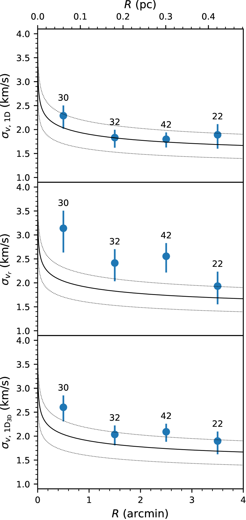
Figure 13: Plot of the one-dimensional tangential velocity dispersion $\sigma_{v,\mathrm{1D}}$ (top), the line of sight velocity dispersion $\sigma_{v_{r}}$ (middle), and the one-dimensional velocity dispersion composed of all three velocity components (assumed isotropic) $\sigma_{v,\mathrm{1D_{3D}}}$ (bottom) as a function of distance from the center of the ONC. Values plotted are listed in Table 4, using an estimated distance to the ONC of $388\pm 5$ pc (Kounkel et al., 2017). The number of sources in each bin is indicated above that bin. The black solid line illustrates the one-dimensional velocity dispersion for virial equilibrium predicted from the stellar and gas mass assuming a spherical potential from Da Rio et al. (2014), and the dashed lines mark the uncertainty assuming a 30% mass error. The Bottom x-axis indicates distance in arcminutes, while the top x-axis indicates distance in pc.

6.2 Effects from the Integral Shaped Filament

The Trapezium sits approximately in the middle of the “integral-shaped filament” (ISF; Bally et al., 1987), a long filament of gas with an approximate “S” shape, and 0.1–0.3 pc in front of the filament (e.g., Baldwin et al., 1991; Wen & O’dell, 1995; O’Dell, 2018; Abel et al., 2019). There has been an observed elongation in the line of sight velocity component, which Stutz & Gould (2016) attributed to interactions with the ISF using APOGEE data. The mechanism put forth by Stutz & Gould (2016) to explain the observed elongation in velocity space is the “slingshot” mechanism, where stars born along the filament could be ejected due to the filament undergoing transverse acceleration while the protostar continually accretes mass. The reason for the ejection is due to the fact that, “when the protostar system becomes sufficiently massive to decouple from the filament, it is released” (Stutz & Gould, 2016). Such a mechanism would provide an additional contribution to a larger velocity dispersion. However, the slingshot mechanism is dependent on the direction of the transverse acceleration of the filament (i.e., along the line of sight or tangential on the plane of the sky). As the filament runs north-south in the region of the Trapezium, this could provide the mechanism for the observed anisotropy in the tangential velocity components, as well as the radial component. This could be an important effect as Stutz & Gould (2016) find the gravity of the background filament likely dominates the gravity field from the stars.

From the analysis of Stutz & Gould (2016), the region we have analyzed here contains primarily stars versus protostars, determined based on their excess IR emission. However, Stutz & Gould (2016) only considered the radial component of motion, and not the tangential components. Additionally, their RV sources were obtained from APOGEE, providing very few sources within the central 0.1 pc of the core region where we observe the highest velocity dispersion along the line of sight. As such, there is additional work to determine how the ISF might work to influence the measured velocity dispersions. Although we do not provide an in-depth theoretical analysis here to compare to observational data, one is warranted.

6.3 Velocity Isotropy

There is a known kinematic anisotropy in the tangential velocities along the north-south direction (e.g., McNamara, 1976; Hillenbrand & Hartmann, 1998; Da Rio et al., 2014; Kim et al., 2019). However, the deviation from tangential to radial (i.e., towards the center of the cluster) anisotropy ($\sigma_{\mathrm{tan}}/\sigma_{\mathrm{rad}}-1$; Bellini et al. 2018) found by Kim et al. (2019) of $0.03\pm 0.04$ is consistent with isotropic velocities in the tangential-radial velocity space. It should be noted that throughout this section, we use “tangential” ($v_{\mathrm{tan}}$) to indicate motion on the plane of the sky, “radial” ($v_{\mathrm{rad}}$) to indicate motion on the plane of the sky pointing towards the cluster center, and “line of sight” ($v_{r}$) to indicate the line of sight (RV) component of motion.

With our three-dimensional kinematic information, we can now compute the ratio of the tangential dispersion to the line of sight dispersion ($\sigma_{v_{\mathrm{1D}}}/\sigma_{v_{r}}$). Figure 14 shows the velocity ratios for $\sigma_{v_{\alpha}}/\sigma_{v_{\delta}}$ (top) and $\sigma_{v_{\mathrm{1D}}}/\sigma_{v_{r}}$ (bottom). The $\sigma_{v_{\alpha}}/\sigma_{v_{\delta}}$ shows a north-south elongation, which is consistent with previous studies, e.g., $\sigma_{\mu_{\alpha\cos\delta}}/\sigma_{\mu_{\delta}}=0.74\pm 0.03$; (Kim et al., 2019); $b/a\approx 0.7$ (Da Rio et al., 2014); see also Jones & Walker (1988) and Kuhn et al. (2019).

We also decomposed tangential velocities to radial ($v_{\mathrm{rad}}$) and tangential ($v_{\mathrm{tan}}$) coordinates, both on the plane of the sky, through a change of basis where the radial axis points towards the ONC CoM. We note that both of these components, $v_{\mathrm{rad}}$ and $v_{\mathrm{tan}}$, are strictly on the plane of the sky and do not include any line of sight velocity component within their vectors. The ratio of $\sigma_{v_{\mathrm{rad}}}/\sigma_{v_{\mathrm{tan}}}$ is shown in Figure 14 (middle), where the majority of points are consistent with isotropic dispersions. We also compare our results to the parent population from Kim et al. (2019, open markers), which shows that our subsample shows variation from the parent population, possibly due to selection effects. Our 1-D tangential to line of sight velocity dispersions ($\sigma_{v_{\mathrm{1D}}}/\sigma_{v_{r}}$) show significant deviation from unity. The combined value for our total sample is $\sigma_{v_{\mathrm{1D}}}/\sigma_{v_{r}}=0.78\pm 0.19$. These measurements may indicate an elongation in the velocities along the line of sight direction.

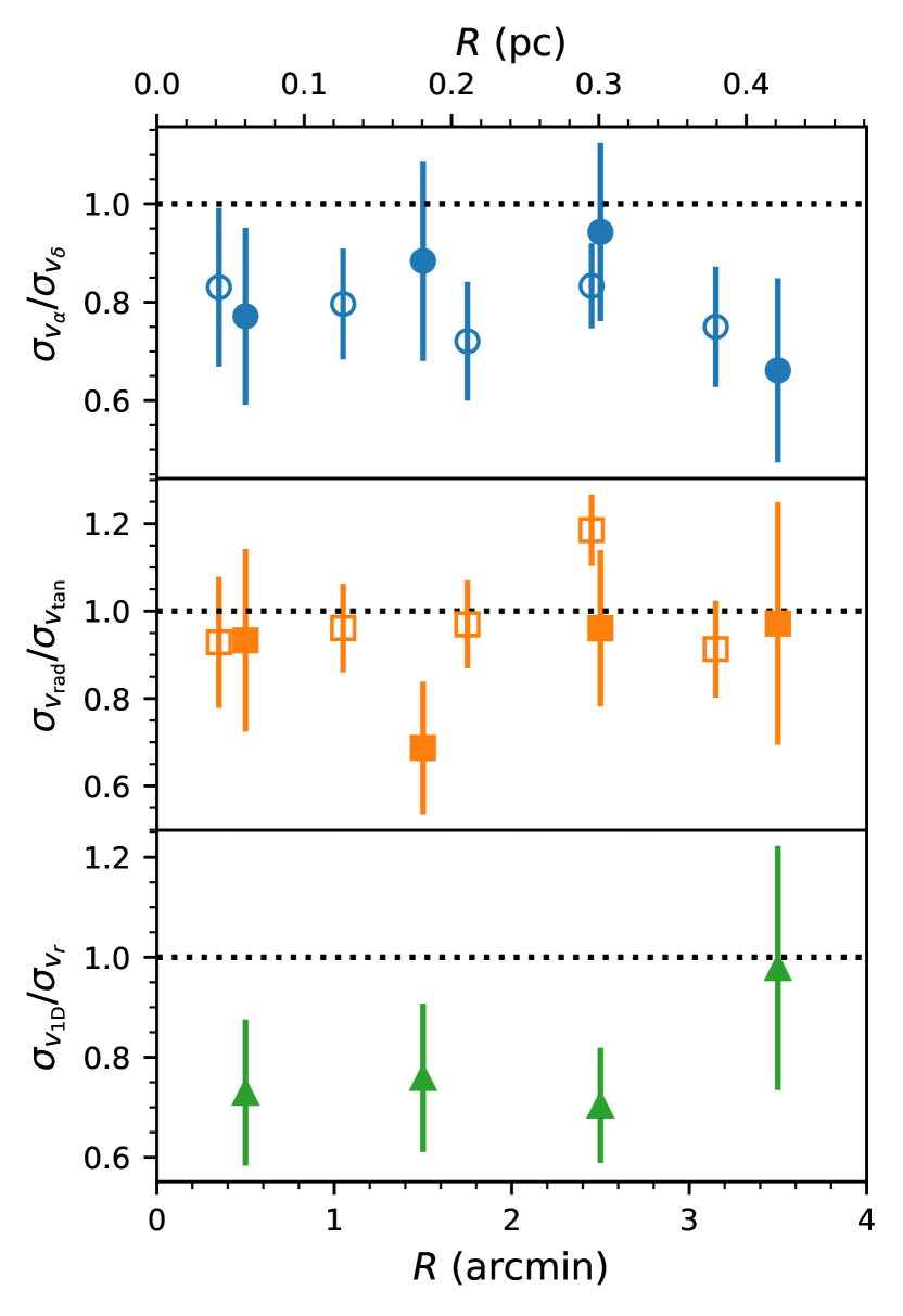
Figure 14: Top: Ratio of east-west to north-south velocity dispersions ($\sigma_{v_{\alpha}}/\sigma_{v_{\delta}}$) as a function of distance from the core of the ONC. Open markers are values from Kim et al. (2019), while closed symbols are from this study. There is a slight north-south elongation that has been found by other studies (e.g., Da Rio et al., 2014; Kim et al., 2019). Middle: Ratio of radial to tangential (vectors on the plane of the sky pointing radially towards the center of the ONC and tangential to that vector) velocity dispersions ($\sigma_{v_{\mathrm{rad}}}/\sigma_{v_{\mathrm{tan}}}$). These components are primarily isotropic, with the exception of the bin between 1′–2′. Bottom: Ratio of tangential to line of sight velocity dispersions ($\sigma_{v_{\mathrm{1D}}}/\sigma_{v_{r}}$). There appears to be a slight elongation in the line of sight direction.

Platais et al. (2020) used a diagram of the angle of the proper motion vector in polar coordinates with respect to the cluster center to examine the how the position vector from the center of the ONC and tangential velocity vector were related for fast moving sources. The expectation is that runwaway stars should have angles between these two vectors close to 0, that is, both the position vector point and proper motion vector point radially away from the center of the ONC. We can use a similar analysis to see if there is preferential motion in the core of the ONC. Figure  15 show the distribution of vectoral angles for all 135 sources in our sample with three components of motion. Random orbits should have no preferential angle, however, there is structure seen in Figure 15. Specifically, there is a preference for sources to have vectoral angles around 90^∘ and $-90^{\circ}$. This corresponds to sources whose motion is tangential to a vector pointing radially away from the center of the ONC (normal vector), possibly indicating that there is a rotational preference for sources in the central ONC. In Figure 15 (bottom) we compare the cumulative distribution of vectoral angles for our 3-D sample to the vectoral angles for all PM sources within 4′ of the ONC CoM from Kim et al. (2019, 671 sources) and a random uniform distribution. The PM sample follows the expected behavior for a random uniform distribution of vectoral angles, which implies a potential bias within our 3-D subsample.

To test for similarity between our 3-D subsample and the parent PM sample from Kim et al. (2019), we performed the Kolmogorov-Smirnov test (K-S test) and the Anderson-Darling test (A-D test). The K-S test gave a test statistic = 0.115 with a p-value = 0.085, which indicates that we can reject the null hypothesis that the two samples come from the same distribution only at an 8.5% probability. The A-D test gave a test statistic = 0.802 with a p-value = 0.153, indicating that we cannot reject that these two distributions are significantly different, similar to the result of the K-S test. Neither of these test results are extremely significant, indicating that the resulting preferential motion of our 3-D sample may not be statistically significant. However, it is worth noting the potential biases introduced into our 3-D subsample versus the Kim et al. (2019) sample.

We also performed a comparison test against a random uniform sample using the same tests mentioned earlier. For our 3-D subsample, the K-S test gave a test statistic = 0.126 with a p-value = 0.023, which indicates that we can reject the null hypothesis that the kinematic sample comes from a uniform distribution at a 2.3% probability. The A-D test gave a test statistic = 1.786 with a p-value = 0.064, which indicates that the null hypothesis can be rejected at the 6.4% level. Again, neither of these test results are extremely significant, motivating the need for a larger kinematic sample within the core. Comparing the parent sample from Kim et al. (2019) to the random distribution gives a K-S test statistic = 0.019 with a p-value = 0.974, and an A-D test statistic = -0.892 with a p-value $>0.25$ (value capped). Both tests indicate that the parent sample is consistent with a random distribution.

Our sample was selected for sources bright enough to be targeted with NIRSPAO (or APOGEE), likely selecting more ONC sources that are in the foreground portion of the cluster rather than deeply embedded sources, which may indicate motion differences as a function of depth in the ONC. Our target list was also curated from the [HC2000] catalog, selecting sources preferentially thought to have masses $\lesssim 1\,M_{\odot}$. It is possible that lower-mass sources are showing different kinematics than the bulk motion within the ONC. Kuhn et al. (2019) attempted to measure the bulk rotation of the ONC using tangential kinematics, but found no significant rotational preference.

It is important to note that this analysis is done assuming all stars are at the same distance. The Gaia satellite (Gaia Collaboration et al., 2016) is currently obtaining parallaxes for over 1 billion sources; however, it has been noted in previous studies that Gaia measurements in the ONC are unreliable due to the high level of nebulosity (e.g., Kim et al., 2019). Indeed, the number of Gaia early Data Release 3 (eDR3; Gaia Collaboration et al., 2021) sources within 1″ of our sources from this study, and consistent within the 2-$\sigma$ combined uncertainty in $\mu_{\alpha}$ and $\mu_{\delta}$ is only three sources. Therefore, a full three-dimensional study of ONC kinematics is not yet possible, and motivates the need for future facilities to obtain parallax measurements for ONC sources.

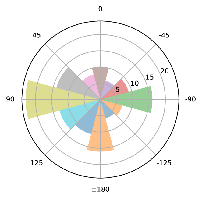
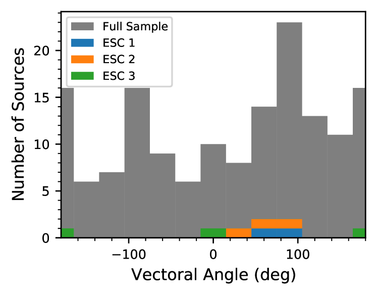
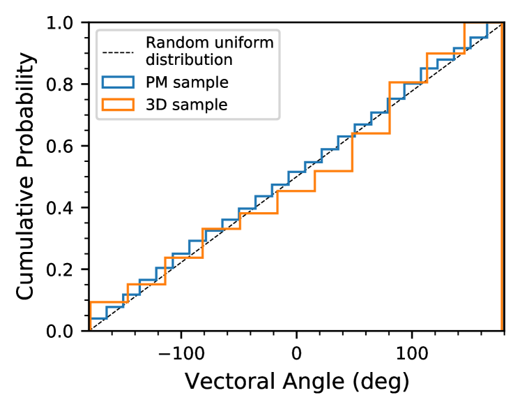
Figure 15: Top: Polar histogram of the angle between the proper motion vector and the radial position vector on the plane of the sky, where an angle of 0 corresponds to both the position vector and velocity vector pointing radially away from the cluster center. Each bin is 30^∘ wide. The radial direction indicates the number of sources in each bin. There is an observed preference for sources to have motion tangential to the core of the ONC (${\sim}\pm 90^{\circ}$), with more sources exhibiting motion +$90^{\circ}$ than $-90^{\circ}$. Middle: The 1-D histogram corresponding to the bins in the polar histogram. We show the vector angles of the escape groups identified in this study and Kim et al. (2019), noting that few of these sources have angles $\sim$0^∘. Bottom: Cumulative probability distributions for our 3-D sample (orange), the entire PM sample within 4′ (blue), and the expected distribution for a random uniform sample (dashed line).

7 Conclusions

Using Keck/NIRSPEC+AO, we have obtained high-precision RV measurements ($\sigma\lesssim 0.5$ km s^-1) for a large number of sources within the core region of the ONC (41 sources within 1′). Additionally, we included a reanalysis of 172 ONC sources observed with SDSS/APOGEE. Using a combined sample of Keck/NIRSPAO, SDSS/APOGEE, and PM measurements from (Kim et al., 2019), for a total sample of 135 sources, we presented a 3-D study of the kinematics of the core population of the ONC. Our main takeaways are the following:

1. Our derived tangential intrinsic velocity dispersions of $\sigma_{v_{\alpha}}=1.64\pm 0.12$ km s^-1 and $\sigma_{v_{\delta}}=2.03\pm 0.13$ km s^-1 are consistent with previous results from the literature, and consistent with the virialized model of the ONC from Da Rio et al. (2014).

2. Our derived line of sight velocity dispersion of $\sigma_{v_{r}}=2.56_{-0.17}^{+0.16}$ km s^-1 is slightly higher than literature estimates. This is potentially due to our sources being concentrated more towards the core of the ONC, which may indicate that the core of the ONC is not yet fully virialized. We explored the possibility that binarity could play a role in creating our larger observed RV dispersions. We simulated different binary fractions, from 0%–100%, and their effect on the observed line of sight velocity dispersion. We found that almost any level of binarity could produce our observed velocity dispersion, however, only a very high level of binarity ($\gtrsim$75%) would make our line of sight velocity dispersion consistent with the observed tangential velocity dispersions. As the binary fraction for the ONC is estimated to be between $\sim$10%–50% (e.g., Reipurth et al., 2007; De Furio et al., 2019; Da Rio et al., 2017), our larger observed RV dispersion is likely not caused by orbital motion in unresolved binaries, and is more likely related to formation/evolution within the ONC.

3. We measure an elongation in the velocity dispersion along the line of sight direction compared to the tangential velocity dispersion, $\sigma_{v_{\mathrm{1D}}}/\sigma_{v_{r}}=0.78\pm 0.19$. This may indicate that there is structure to the velocities of stars in the ONC, or possibly a result of the “slingshot” mechanism from the background filament (Stutz & Gould, 2016; Stutz, 2018). The ratio of tangential velocity dispersions $\sigma_{v_{\alpha}}/\sigma_{v_{\delta}}$ shows a north-south elongation which is consistent with previous studies (e.g., Da Rio et al., 2014; Kim et al., 2019), and tends to run along the filament. However, the tangential to radial (towards the center of the ONC) velocity dispersions $\sigma_{v_{\mathrm{1D}}}/\sigma_{v_{r}}$ appear consistent with unity, as other studies have noted (e.g., Da Rio et al., 2014; Kim et al., 2019).

4. We observe two additional potential kinematic outlier sources (escaping/evaporating) based on their RVs from APOGEE (2MASS 05351906$-$0523495 and 2MASS 05352321$-$0521357). However, their large line of sight velocities may also be due to binarity, and additional follow up is needed to confirm if their velocities are truly elevated.

5. There is a somewhat low probability that the 3-D sample is drawn from a uniform distribution, which could indicate a rotational preference on the plane of the sky, as indicated by the angles between sources position vectors and tangential motion vectors. However, the parent population of Kim et al. (2019) is consistent with a uniform distribution, i.e. no rotational preference. We find that both our 3-D sample and the Kim et al. (2019) sample are relatively consistent, therefore, we cannot rule out the null hypothesis that both populations are consistent with a uniform distribution. A larger sample with higher precision measurements is likely required to further investigate the bulk rotation of the ONC core.

Our study indicates that additional AO imaging and/or extremely high-resolution spectroscopy is necessary to increase the sample size and reduce uncertainties to determine if the core of the ONC is virialized and/or shows significant velocity structure. This will allow for a comprehensive study of the 3-D kinematics of the ONC to better understand the difference between tangential velocities and line of sight velocities. Future work is required to compare data to detailed simulations (e.g., Kroupa, 2000; McKee & Tan, 2002, 2003; Proszkow et al., 2009; Krumholz et al., 2011, 2012; Kuznetsova et al., 2015, 2018) to determine the dynamical state of the ONC.

Appendix A APOGEE Results

Table 5 shows the results of our forward-modeling pipeline applied to our APOGEE sources (see Section 4).

Table 5: APOGEE Forward-Modeling Results

APOGEE ID	ID	$\alpha_{J2000}$	$\delta_{J2000}$	$\overline{RV}$	$\mu_{\alpha\cos\delta}$	$\mu_{\delta}$	$T_{\mathrm{eff}}$	$v\sin{i}$	Veiling	Note
		(deg)	(deg)	(km s-1)	(mas yr-1)	(mas yr-1)	(K)	(km s-1)	$\left(\dfrac{F_{H,\mathrm{cont}}}{F_{H,\ast}}\right)$
2M05350101-0524103	663	$83.75420833$	$-5.40286111$	$31.46\pm 0.19$	$0.16\pm 0.07$	$-0.62\pm 0.14$	$3825.01\pm 12.53$	$38.23\pm 0.92$	0.56	C
2M05350117-0524067	$\cdots$	$83.75487500$	$-5.40186111$	$25.59\pm 0.18$	$\cdots$	$\cdots$	$3979\pm 6$	$5.40\pm 1.00$	0.51
2M05350160-0524101	655	$83.75666667$	$-5.40280556$	$27.82\pm 0.24$	$1.21\pm 0.29$	$0.25\pm 0.27$	$2908.02\pm 9.21$	$35.18\pm 0.88$	0.36
2M05350284-0522082	140	$83.76183333$	$-5.36894444$	$25.49\pm 0.14$	$-0.96\pm 0.15$	$-1.85\pm 0.31$	$5100.45\pm 1.56$	$27.43\pm 0.36$	0.58
2M05350309-0522378	190	$83.76287500$	$-5.37716667$	$29.98\pm 1.67$	$-0.20\pm 0.38$	$1.01\pm 0.05$	$3057.64\pm 30.73$	$15.65\pm 0.39$	0.39
2M05350370-0522457	189	$83.76541667$	$-5.37936111$	$31.37\pm 0.57$	$-0.13\pm 0.48$	$-0.16\pm 0.19$	$3138.91\pm 23.35$	$12.69\pm 0.50$	0.50
2M05350437-0523138	11	$83.76820833$	$-5.38716667$	$24.65\pm 1.29$	$0.42\pm 0.16$	$0.95\pm 0.05$	$4107.19\pm 63.65$	$17.67\pm 1.21$	1.04
2M05350450-0523565	$\cdots$	$83.76875000$	$-5.39902778$	$33.82\pm 0.92$	$\cdots$	$\cdots$	$4591\pm 7$	$27.77\pm 1.63$	0.85
2M05350461-0524424	657	$83.76920833$	$-5.41177778$	$26.44\pm 0.44$	$0.12\pm 0.10$	$-0.86\pm 0.08$	$3988.02\pm 9.04$	$16.79\pm 0.40$	0.42
2M05350481-0522387	67	$83.77004167$	$-5.37741667$	$26.95\pm 1.16$	$0.63\pm 0.01$	$1.26\pm 0.11$	$3544.42\pm 5.64$	$10.52\pm 2.27$	0.67
2M05350487-0520574	542	$83.77029167$	$-5.34927778$	$29.34\pm 0.57$	$0.25\pm 0.15$	$-0.23\pm 0.25$	$3733.67\pm 7.92$	$11.91\pm 0.53$	0.62
2M05350495-0521092	3	$83.77062500$	$-5.35255556$	$29.75\pm 0.41$	$-0.43\pm 0.06$	$2.12\pm 0.18$	$4119.19\pm 13.19$	$13.71\pm 1.44$	0.59
2M05350513-0520244	564	$83.77137500$	$-5.34011111$	$26.75\pm 0.28$	$-0.38\pm 0.46$	$-0.42\pm 0.18$	$4126.16\pm 10.04$	$9.15\pm 0.44$	0.53
2M05350537-0524105	77	$83.77237500$	$-5.40291667$	$26.33\pm 0.87$	$0.14\pm 0.36$	$-0.19\pm 0.08$	$4249.94\pm 50.38$	$16.20\pm 0.36$	0.95
2M05350540-0524150	176	$83.77250000$	$-5.40416667$	$24.40\pm 0.28$	$0.95\pm 0.25$	$1.04\pm 0.23$	$3686.05\pm 23.07$	$4.84\pm 1.85$	1.51
2M05350563-0525195	$\cdots$	$83.77345833$	$-5.42208333$	$28.83\pm 0.52$	$\cdots$	$\cdots$	$4582\pm 10$	$42.24\pm 0.81$	1.05
2M05350568-0525058	656	$83.77366667$	$-5.41827778$	$27.17\pm 0.29$	$-1.38\pm 0.27$	$-0.16\pm 0.11$	$4205.50\pm 8.81$	$99.00\pm 0.87$	0.16
2M05350571-0523540	39	$83.77379167$	$-5.39833333$	$23.77\pm 0.22$	$-1.04\pm 0.47$	$-0.84\pm 0.05$	$3029.62\pm 6.43$	$21.64\pm 0.16$	0.42
2M05350617-0522124	264	$83.77570833$	$-5.37011111$	$29.26\pm 0.24$	$-0.85\pm 0.39$	$-0.75\pm 0.16$	$3828.14\pm 7.31$	$9.69\pm 1.16$	0.51	C
2M05350627-0522027	129	$83.77612500$	$-5.36741667$	$27.96\pm 0.23$	$-0.32\pm 0.24$	$0.11\pm 0.34$	$4450.92\pm 6.15$	$27.39\pm 0.27$	0.24
2M05350651-0524414	$\cdots$	$83.77712500$	$-5.41150000$	$25.72\pm 0.22$	$\cdots$	$\cdots$	$4269\pm 7$	$21.56\pm 0.07$	0.24
2M05350727-0522266	131	$83.78029167$	$-5.37405556$	$25.99\pm 0.27$	$0.24\pm 0.09$	$-0.66\pm 0.78$	$3163.11\pm 37.48$	$13.13\pm 0.47$	0.39
2M05350739-0525481	585	$83.78079167$	$-5.43002778$	$25.80\pm 0.30$	$-0.16\pm 0.06$	$0.27\pm 0.05$	$2814.95\pm 17.31$	$9.62\pm 0.98$	0.41
2M05350773-0521014	629	$83.78220833$	$-5.35038889$	$28.70\pm 0.30$	$-0.56\pm 0.16$	$-1.30\pm 0.13$	$4326.53\pm 15.17$	$24.86\pm 0.97$	1.14
2M05350822-0524032	679	$83.78425000$	$-5.40088889$	$26.43\pm 0.26$	$1.14\pm 0.13$	$1.47\pm 0.22$	$3168.52\pm 7.79$	$6.48\pm 1.30$	0.76
2M05350829-0524348	17	$83.78454167$	$-5.40966667$	$25.05\pm 0.29$	$-0.57\pm 0.46$	$0.12\pm 0.01$	$3064.95\pm 8.25$	$7.43\pm 0.69$	0.51
2M05350853-0524411	171	$83.78554167$	$-5.41141667$	$31.54\pm 1.53$	$-1.82\pm 0.73$	$-0.07\pm 0.18$	$3048.41\pm 28.89$	$10.95\pm 0.62$	0.52	C
2M05350853-0525179	$\cdots$	$83.78554167$	$-5.42163889$	$23.35\pm 0.19$	$\cdots$	$\cdots$	$4016\pm 8$	$5.69\pm 0.50$	0.51
2M05350859-0526194	$\cdots$	$83.78579167$	$-5.43872222$	$26.43\pm 0.43$	$\cdots$	$\cdots$	$2977\pm 11$	$14.62\pm 0.66$	0.29
2M05350873-0522566	50	$83.78637500$	$-5.38238889$	$26.21\pm 0.26$	$1.05\pm 0.42$	$-1.26\pm 0.26$	$4198.10\pm 10.63$	$71.75\pm 0.89$	0.32
2M05350976-0521282	58	$83.79066667$	$-5.35783333$	$27.32\pm 0.40$	$-1.15\pm 0.21$	$-2.57\pm 0.29$	$4372.17\pm 6.81$	$27.20\pm 0.14$	0.16
2M05350992-0521433	359	$83.79133333$	$-5.36202778$	$28.57\pm 0.71$	$-1.17\pm 0.06$	$-0.23\pm 0.48$	$4131.49\pm 32.85$	$14.92\pm 1.73$	1.03
2M05351014-0522326	46	$83.79225000$	$-5.37572222$	$28.82\pm 0.27$	$-1.02\pm 0.20$	$0.73\pm 0.26$	$4021.55\pm 10.76$	$24.02\pm 1.33$	0.64
2M05351021-0523215	169	$83.79254167$	$-5.38930556$	$25.51\pm 0.34$	$1.31\pm 0.63$	$-0.86\pm 0.43$	$4329.25\pm 7.55$	$15.92\pm 0.45$	0.98
2M05351029-0519563	550	$83.79287500$	$-5.33230556$	$26.54\pm 0.32$	$-1.68\pm 0.11$	$1.67\pm 0.10$	$3449.75\pm 9.32$	$24.33\pm 0.54$	0.54
2M05351031-0521130	519	$83.79295833$	$-5.35361111$	$27.14\pm 0.15$	$1.14\pm 0.07$	$-0.36\pm 0.12$	$4165.05\pm 7.13$	$8.73\pm 1.04$	0.69
2M05351041-0519523	552	$83.79337500$	$-5.33119444$	$27.39\pm 0.55$	$0.82\pm 0.12$	$-1.53\pm 0.17$	$3445.06\pm 43.97$	$19.36\pm 0.24$	0.54
2M05351047-0526003	595	$83.79362500$	$-5.43341667$	$27.74\pm 2.66$	$-0.59\pm 0.35$	$-0.20\pm 0.52$	$2722.45\pm 220.03$	$19.91\pm 1.37$	0.04
2M05351050-0522455	6	$83.79375000$	$-5.37930556$	$24.86\pm 0.29$	$0.14\pm 0.46$	$-1.53\pm 0.06$	$4125.77\pm 7.78$	$44.03\pm 0.13$	0.36
2M05351050-0526183	$\cdots$	$83.79375000$	$-5.43841667$	$22.61\pm 0.26$	$\cdots$	$\cdots$	$4504\pm 8$	$23.52\pm 0.23$	0.50
2M05351053-0522166	262	$83.79387500$	$-5.37127778$	$27.55\pm 0.28$	$-0.91\pm 0.25$	$0.89\pm 0.10$	$3728.33\pm 8.85$	$23.61\pm 0.36$	0.66
2M05351061-0522559	251	$83.79420833$	$-5.38219444$	$26.01\pm 1.01$	$-0.37\pm 0.15$	$-0.24\pm 0.10$	$4244.42\pm 76.70$	$22.11\pm 1.01$	0.89
2M05351073-0526280	$\cdots$	$83.79470833$	$-5.44111111$	$28.03\pm 0.26$	$\cdots$	$\cdots$	$3804\pm 9$	$18.25\pm 0.47$	0.64
2M05351083-0525569	594	$83.79512500$	$-5.43247222$	$27.93\pm 0.96$	$0.58\pm 0.30$	$2.74\pm 0.45$	$2924.92\pm 41.45$	$15.96\pm 1.17$	0.56
2M05351094-0524486	489	$83.79558333$	$-5.41350000$	$24.98\pm 1.48$	$2.04\pm 0.72$	$1.94\pm 0.31$	$3716.95\pm 51.72$	$28.31\pm 0.28$	0.90	C
2M05351149-0526023	$\cdots$	$83.79787500$	$-5.43397222$	$19.04\pm 0.18$	$\cdots$	$\cdots$	$4370\pm 6$	$42.42\pm 1.60$	0.16
2M05351163-0522515	75	$83.79845833$	$-5.38097222$	$25.36\pm 0.24$	$-0.04\pm 0.79$	$-0.20\pm 0.24$	$3054.10\pm 16.36$	$11.06\pm 1.01$	0.99
2M05351165-0524213	191	$83.79854167$	$-5.40591667$	$25.25\pm 0.14$	$0.34\pm 0.13$	$-0.52\pm 0.14$	$3029.60\pm 7.19$	$12.41\pm 0.51$	0.86
2M05351178-0521555	150	$83.79908333$	$-5.36541667$	$26.84\pm 1.28$	$-0.03\pm 0.66$	$-0.30\pm 0.94$	$2929.69\pm 8.11$	$12.07\pm 1.17$	0.51
2M05351188-0521032	38	$83.79950000$	$-5.35088889$	$27.48\pm 0.24$	$-0.25\pm 0.15$	$0.33\pm 0.52$	$4292.95\pm 5.88$	$10.65\pm 0.48$	0.74	C
2M05351197-0522541	248	$83.79987500$	$-5.38169444$	$93.82\pm 39.46$	$0.82\pm 0.57$	$-0.00\pm 0.53$	$3781.89\pm 82.67$	$255.27\pm 23.13$	7.21
2M05351227-0520452	526	$83.80112500$	$-5.34588889$	$28.05\pm 1.13$	$1.26\pm 0.34$	$0.46\pm 0.36$	$3351.49\pm 12.02$	$7.51\pm 0.52$	0.78
2M05351227-0523479	$\cdots$	$83.80112500$	$-5.39663889$	$27.37\pm 0.23$	$\cdots$	$\cdots$	$4216\pm 6$	$12.34\pm 0.31$	0.37
2M05351259-0523440	$\cdots$	$83.80245833$	$-5.39555556$	$27.42\pm 1.27$	$\cdots$	$\cdots$	$4445\pm 8$	$41.44\pm 0.64$	0.45
2M05351269-0519353	$\cdots$	$83.80287500$	$-5.32647222$	$30.15\pm 0.19$	$\cdots$	$\cdots$	$3713\pm 13$	$7.39\pm 0.87$	0.58
2M05351277-0520349	56	$83.80320833$	$-5.34302778$	$21.73\pm 0.65$	$0.71\pm 0.15$	$0.71\pm 0.20$	$3054.25\pm 12.07$	$13.47\pm 0.89$	1.08
2M05351304-0520302	554	$83.80433333$	$-5.34172222$	$30.84\pm 0.43$	$-1.30\pm 0.19$	$1.12\pm 0.31$	$4249.74\pm 6.80$	$19.38\pm 0.23$	0.31
2M05351305-0521532	261	$83.80437500$	$-5.36477778$	$29.92\pm 0.24$	$-1.65\pm 0.05$	$-1.42\pm 0.04$	$3825.16\pm 14.48$	$9.99\pm 1.21$	1.40
2M05351319-0524554	$\cdots$	$83.80495833$	$-5.41538889$	$25.21\pm 0.33$	$\cdots$	$\cdots$	$4296\pm 9$	$26.69\pm 0.38$	0.95
2M05351330-0520189	109	$83.80541667$	$-5.33858333$	$29.60\pm 0.21$	$-0.02\pm 0.26$	$1.56\pm 2.06$	$4048.63\pm 5.49$	$42.23\pm 0.23$	0.44
2M05351336-0522261	53	$83.80566667$	$-5.37391667$	$25.87\pm 1.45$	$2.45\pm 0.36$	$1.29\pm 0.33$	$3631.97\pm 60.91$	$13.81\pm 1.69$	1.30
2M05351343-0521073	377	$83.80595833$	$-5.35202778$	$30.99\pm 0.22$	$0.88\pm 0.05$	$-0.94\pm 0.07$	$3814.00\pm 12.61$	$3.85\pm 1.61$	1.27
2M05351352-0522195	146	$83.80633333$	$-5.37208333$	$31.09\pm 0.54$	$-0.70\pm 0.14$	$-1.02\pm 0.32$	$4058.32\pm 17.56$	$16.49\pm 0.39$	0.85
2M05351362-0519548	$\cdots$	$83.80675000$	$-5.33188889$	$30.67\pm 1.39$	$\cdots$	$\cdots$	$4405\pm 30$	$23.53\pm 0.87$	0.41
2M05351379-0519254	$\cdots$	$83.80745833$	$-5.32372222$	$23.99\pm 0.24$	$\cdots$	$\cdots$	$2838\pm 7$	$15.29\pm 0.92$	0.37
2M05351397-0521233	117	$83.80820833$	$-5.35647222$	$24.02\pm 0.21$	$1.21\pm 0.49$	$-0.58\pm 0.23$	$4053.25\pm 13.71$	$9.09\pm 0.41$	0.95
2M05351405-0519520	$\cdots$	$83.80854167$	$-5.33111111$	$23.78\pm 0.15$	$\cdots$	$\cdots$	$4267\pm 7$	$12.32\pm 0.28$	0.68
2M05351405-0523383	507	$83.80854167$	$-5.39397222$	$24.91\pm 0.33$	$0.07\pm 0.12$	$0.44\pm 0.01$	$3921.76\pm 8.73$	$60.27\pm 0.44$	0.35
2M05351421-0520042	$\cdots$	$83.80920833$	$-5.33450000$	$26.68\pm 0.30$	$\cdots$	$\cdots$	$4091\pm 12$	$12.38\pm 0.40$	0.85
2M05351427-0524246	$\cdots$	$83.80945833$	$-5.40683333$	$27.94\pm 0.80$	$\cdots$	$\cdots$	$4285\pm 20$	$50.89\pm 0.46$	0.41
2M05351439-0523335	521	$83.80995833$	$-5.39263889$	$26.01\pm 0.79$	$-0.11\pm 0.23$	$-1.65\pm 0.03$	$4130.95\pm 25.34$	$27.82\pm 0.55$	0.66
2M05351465-0523018	236	$83.81104167$	$-5.38383333$	$30.78\pm 0.31$	$1.17\pm 0.69$	$-0.94\pm 0.35$	$4038.46\pm 12.69$	$14.62\pm 0.46$	0.78
2M05351471-0521063	319	$83.81129167$	$-5.35175000$	$29.72\pm 0.85$	$-0.58\pm 0.02$	$-0.82\pm 0.05$	$4354.13\pm 28.40$	$17.89\pm 0.69$	0.43
2M05351498-0521598	567	$83.81241667$	$-5.36661111$	$29.14\pm 0.38$	$2.25\pm 0.09$	$0.96\pm 0.11$	$4417.59\pm 8.65$	$21.56\pm 0.06$	0.25	V
2M05351554-0525140	$\cdots$	$83.81475000$	$-5.42055556$	$36.71\pm 1.67$	$\cdots$	$\cdots$	$4277\pm 9$	$95.71\pm 0.60$	0.21
2M05351561-0524030	37	$83.81504167$	$-5.40083333$	$29.62\pm 1.23$	$0.54\pm 0.11$	$-1.80\pm 0.02$	$4389.08\pm 10.23$	$60.37\pm 0.94$	0.19
2M05351563-0522565	$\cdots$	$83.81512500$	$-5.38236111$	$30.29\pm 1.22$	$\cdots$	$\cdots$	$4468\pm 6$	$28.65\pm 0.32$	0.54
2M05351567-0525331	616	$83.81529167$	$-5.42586111$	$25.57\pm 0.48$	$0.09\pm 0.20$	$-0.74\pm 0.11$	$3951.44\pm 9.34$	$22.09\pm 0.74$	1.38
2M05351571-0526283	$\cdots$	$83.81545833$	$-5.44119444$	$25.79\pm 1.34$	$\cdots$	$\cdots$	$3875\pm 37$	$8.89\pm 1.08$	0.67
2M05351587-0522328	241	$83.81612500$	$-5.37577778$	$30.63\pm 1.45$	$0.24\pm 0.15$	$1.21\pm 0.17$	$3022.39\pm 39.10$	$8.83\pm 1.63$	1.35
2M05351606-0520363	517	$83.81691667$	$-5.34341667$	$23.56\pm 0.22$	$0.55\pm 0.25$	$1.44\pm 0.24$	$4163.85\pm 8.74$	$16.04\pm 1.49$	0.83
2M05351609-0524112	173	$83.81704167$	$-5.40311111$	$23.01\pm 0.24$	$-1.73\pm 0.13$	$-0.79\pm 0.12$	$3463.66\pm 13.22$	$33.20\pm 0.69$	0.90
2M05351661-0519357	$\cdots$	$83.81920833$	$-5.32658333$	$28.54\pm 0.36$	$\cdots$	$\cdots$	$4098\pm 11$	$19.85\pm 0.33$	0.94
2M05351671-0522309	175	$83.81962500$	$-5.37525000$	$29.02\pm 0.28$	$0.65\pm 0.11$	$1.33\pm 0.18$	$3659.32\pm 26.94$	$11.82\pm 1.24$	1.99
2M05351694-0525469	451	$83.82058333$	$-5.42969444$	$29.40\pm 0.37$	$0.31\pm 0.04$	$-0.91\pm 0.06$	$3660.92\pm 13.75$	$54.77\pm 1.18$	0.95
2M05351697-0521452	$\cdots$	$83.82070833$	$-5.36255556$	$47.39\pm 3.56$	$\cdots$	$\cdots$	$6998\pm 2$	$299.48\pm 0.88$	0.10
2M05351697-0523009	560	$83.82070833$	$-5.38358333$	$33.28\pm 0.30$	$0.78\pm 0.13$	$1.15\pm 0.04$	$4228.79\pm 6.23$	$29.65\pm 0.73$	0.59
2M05351712-0524585	331	$83.82133333$	$-5.41625000$	$26.60\pm 0.25$	$-0.80\pm 0.29$	$-0.85\pm 0.07$	$3023.52\pm 7.83$	$15.66\pm 0.29$	0.39
2M05351722-0520277	529	$83.82175000$	$-5.34102778$	$24.01\pm 1.76$	$-0.22\pm 0.09$	$-0.27\pm 0.12$	$3812.67\pm 11.91$	$13.15\pm 1.46$	0.82
2M05351734-0522357	$\cdots$	$83.82225000$	$-5.37658333$	$28.46\pm 2.12$	$\cdots$	$\cdots$	$4504\pm 71$	$32.52\pm 2.03$	1.00
2M05351736-0520149	505	$83.82233333$	$-5.33747222$	$27.15\pm 0.44$	$-0.71\pm 0.16$	$-0.31\pm 0.12$	$4078.60\pm 11.35$	$7.13\pm 0.85$	0.64
2M05351736-0525446	619	$83.82233333$	$-5.42905556$	$27.12\pm 0.40$	$0.93\pm 0.10$	$0.24\pm 0.10$	$4098.05\pm 10.50$	$8.37\pm 1.64$	0.47	C
2M05351754-0525427	618	$83.82308333$	$-5.42852778$	$24.34\pm 0.25$	$-1.00\pm 0.15$	$-0.39\pm 0.17$	$4185.24\pm 10.90$	$23.47\pm 0.32$	0.57
2M05351778-0523155	183	$83.82408333$	$-5.38763889$	$25.69\pm 0.55$	$-1.61\pm 0.17$	$0.60\pm 0.38$	$4098.62\pm 13.74$	$18.31\pm 0.61$	0.53	C
2M05351794-0525061	440	$83.82475000$	$-5.41836111$	$31.16\pm 19.24$	$-0.19\pm 0.28$	$-1.11\pm 0.43$	$2739.27\pm 172.56$	$17.45\pm 117.44$	0.87
2M05351794-0525338	453	$83.82475000$	$-5.42605556$	$26.73\pm 0.50$	$0.50\pm 0.04$	$1.11\pm 2.80$	$3638.90\pm 8.83$	$27.37\pm 0.38$	0.73
2M05351797-0526506	$\cdots$	$83.82487500$	$-5.44738889$	$25.16\pm 0.32$	$\cdots$	$\cdots$	$2961\pm 14$	$7.41\pm 0.63$	0.51
2M05351820-0524302	112	$83.82583333$	$-5.40838889$	$25.21\pm 1.62$	$0.79\pm 0.19$	$2.27\pm 0.12$	$2858.10\pm 13.45$	$39.54\pm 0.91$	0.75
2M05351836-0524267	88	$83.82650000$	$-5.40741667$	$25.50\pm 0.26$	$-1.00\pm 0.31$	$0.31\pm 0.10$	$3120.85\pm 10.14$	$2.44\pm 1.38$	0.90
2M05351846-0524068	506	$83.82691667$	$-5.40188889$	$27.13\pm 0.21$	$-0.17\pm 0.42$	$0.43\pm 0.17$	$3849.71\pm 9.16$	$19.76\pm 0.22$	0.84
2M05351851-0520427	119	$83.82712500$	$-5.34519444$	$31.06\pm 1.62$	$-1.70\pm 0.12$	$0.60\pm 0.22$	$3685.33\pm 15.17$	$50.66\pm 0.60$	0.73
2M05351858-0526248	$\cdots$	$83.82741667$	$-5.44022222$	$24.92\pm 7.93$	$\cdots$	$\cdots$	$3832\pm 102$	$3.11\pm 28.24$	1.36
2M05351866-0523139	$\cdots$	$83.82775000$	$-5.38719444$	$31.91\pm 0.28$	$\cdots$	$\cdots$	$5103\pm 5$	$39.12\pm 1.17$	1.21
2M05351884-0522229	20	$83.82850000$	$-5.37302778$	$23.73\pm 0.91$	$0.14\pm 0.20$	$-0.04\pm 0.15$	$3721.33\pm 235.56$	$15.83\pm 7.06$	1.58
2M05351894-0520522	549	$83.82891667$	$-5.34783333$	$24.41\pm 0.15$	$1.72\pm 0.29$	$-0.99\pm 0.15$	$4035.02\pm 13.79$	$11.85\pm 1.22$	2.06
2M05351906-0523495	148	$83.82941667$	$-5.39708333$	$45.52\pm 1.25$	$1.86\pm 0.36$	$-1.37\pm 1.24$	$4429.27\pm 17.62$	$53.25\pm 3.39$	0.83	E3
2M05351913-0520387	$\cdots$	$83.82970833$	$-5.34408333$	$37.94\pm 8.57$	$\cdots$	$\cdots$	$6996\pm 4$	$299.17\pm 0.99$	0.47
2M05351930-0520078	$\cdots$	$83.83041667$	$-5.33550000$	$32.90\pm 1.78$	$\cdots$	$\cdots$	$6273\pm 91$	$117.19\pm 10.98$	0.75
2M05351965-0524266	573	$83.83187500$	$-5.40738889$	$23.19\pm 0.20$	$0.33\pm 0.34$	$-0.29\pm 0.09$	$3946.35\pm 9.24$	$18.18\pm 0.34$	1.10
2M05352004-0521059	$\cdots$	$83.83350000$	$-5.35163889$	$37.13\pm 0.21$	$\cdots$	$\cdots$	$4437\pm 7$	$48.90\pm 0.42$	0.27
2M05352004-0525375	$\cdots$	$83.83350000$	$-5.42708333$	$26.74\pm 0.66$	$\cdots$	$\cdots$	$4135\pm 33$	$11.75\pm 0.79$	0.56
2M05352016-0526390	$\cdots$	$83.83400000$	$-5.44416667$	$29.18\pm 1.03$	$\cdots$	$\cdots$	$4422\pm 8$	$53.50\pm 1.09$	0.15
2M05352017-0523085	441	$83.83404167$	$-5.38569444$	$29.24\pm 1.64$	$-2.14\pm 0.69$	$-0.87\pm 0.29$	$3867.80\pm 12.47$	$40.21\pm 1.46$	0.95
2M05352054-0524208	104	$83.83558333$	$-5.40577778$	$27.47\pm 0.21$	$-0.58\pm 0.20$	$-0.92\pm 0.05$	$3572.29\pm 50.85$	$7.87\pm 1.48$	1.64
2M05352056-0520431	192	$83.83566667$	$-5.34530556$	$29.39\pm 1.53$	$-0.29\pm 0.05$	$0.28\pm 0.82$	$3498.69\pm 252.68$	$17.07\pm 1.19$	0.55
2M05352067-0523531	72	$83.83612500$	$-5.39808333$	$25.70\pm 0.20$	$0.09\pm 0.12$	$0.31\pm 0.05$	$2978.36\pm 7.07$	$10.68\pm 1.18$	0.30
2M05352076-0521550	$\cdots$	$83.83650000$	$-5.36527778$	$25.24\pm 1.53$	$\cdots$	$\cdots$	$4288\pm 14$	$10.22\pm 0.71$	0.58
2M05352082-0521216	34	$83.83675000$	$-5.35600000$	$32.46\pm 0.26$	$0.70\pm 2.17$	$0.83\pm 0.91$	$4020.81\pm 16.31$	$35.50\pm 1.37$	1.42
2M05352103-0522250	86	$83.83762500$	$-5.37361111$	$27.16\pm 0.18$	$-1.02\pm 0.09$	$1.41\pm 0.72$	$3725.53\pm 8.10$	$16.62\pm 0.72$	0.83
2M05352104-0523490	$\cdots$	$83.83766667$	$-5.39694444$	$31.25\pm 0.23$	$\cdots$	$\cdots$	$4503\pm 10$	$54.80\pm 0.31$	0.12	V
2M05352115-0525569	612	$83.83812500$	$-5.43247222$	$22.19\pm 0.23$	$1.04\pm 0.26$	$-0.11\pm 0.16$	$4107.03\pm 7.56$	$29.68\pm 0.54$	0.45
2M05352139-0526439	$\cdots$	$83.83912500$	$-5.44552778$	$26.03\pm 0.21$	$\cdots$	$\cdots$	$4386\pm 7$	$19.74\pm 0.17$	0.13
2M05352162-0526576	$\cdots$	$83.84008333$	$-5.44933333$	$30.06\pm 1.01$	$\cdots$	$\cdots$	$3061\pm 9$	$72.25\pm 0.95$	0.33
2M05352166-0525264	$\cdots$	$83.84025000$	$-5.42400000$	$25.74\pm 0.18$	$\cdots$	$\cdots$	$4209\pm 12$	$12.44\pm 1.36$	0.59
2M05352172-0526443	617	$83.84050000$	$-5.44563889$	$26.49\pm 0.63$	$1.05\pm 0.06$	$1.38\pm 0.03$	$3749.12\pm 8.63$	$16.95\pm 0.86$	0.61
2M05352181-0523539	139	$83.84087500$	$-5.39830556$	$25.79\pm 1.28$	$0.98\pm 0.09$	$0.84\pm 0.21$	$4535.92\pm 8.94$	$48.97\pm 0.50$	0.14
2M05352184-0522082	89	$83.84100000$	$-5.36894444$	$26.71\pm 0.27$	$0.15\pm 0.29$	$1.13\pm 0.13$	$4067.68\pm 11.01$	$23.87\pm 0.50$	0.44
2M05352208-0524327	145	$83.84200000$	$-5.40908333$	$23.37\pm 0.20$	$1.36\pm 0.47$	$-1.32\pm 0.33$	$3257.96\pm 8.18$	$12.89\pm 0.68$	0.71
2M05352219-0526373	$\cdots$	$83.84245833$	$-5.44369444$	$29.56\pm 0.31$	$\cdots$	$\cdots$	$4246\pm 7$	$34.67\pm 0.10$	0.13
2M05352226-0520292	$\cdots$	$83.84275000$	$-5.34144444$	$23.37\pm 0.34$	$\cdots$	$\cdots$	$4526\pm 6$	$13.41\pm 0.83$	0.08
2M05352244-0522010	558	$83.84350000$	$-5.36694444$	$22.86\pm 0.29$	$0.03\pm 0.09$	$-1.20\pm 0.11$	$4467.55\pm 7.58$	$19.88\pm 1.08$	0.36
2M05352246-0525451	652	$83.84358333$	$-5.42919444$	$30.53\pm 0.41$	$-2.23\pm 0.31$	$-1.26\pm 0.45$	$3544.14\pm 12.54$	$14.72\pm 0.88$	0.91
2M05352274-0519478	$\cdots$	$83.84475000$	$-5.32994444$	$30.20\pm 0.22$	$\cdots$	$\cdots$	$4292\pm 12$	$31.28\pm 0.39$	0.46
2M05352296-0522415	551	$83.84566667$	$-5.37819444$	$28.32\pm 1.53$	$-0.59\pm 0.13$	$2.26\pm 0.07$	$4477.92\pm 8.26$	$66.41\pm 0.82$	0.07
2M05352317-0522283	623	$83.84654167$	$-5.37452778$	$25.57\pm 0.31$	$-0.28\pm 0.19$	$-0.09\pm 0.21$	$3933.29\pm 12.09$	$3.56\pm 1.35$	1.10
2M05352321-0521357	535	$83.84670833$	$-5.35991667$	$47.65\pm 0.56$	$-1.26\pm 0.21$	$-1.92\pm 0.20$	$3132.12\pm 14.43$	$53.83\pm 1.35$	1.11	E3
2M05352332-0521254	556	$83.84716667$	$-5.35705556$	$29.54\pm 0.34$	$1.51\pm 0.23$	$-0.34\pm 0.22$	$4235.67\pm 10.56$	$11.89\pm 1.41$	1.17
2M05352349-0520016	$\cdots$	$83.84787500$	$-5.33377778$	$26.49\pm 1.78$	$\cdots$	$\cdots$	$4058\pm 27$	$53.43\pm 1.19$	0.55
2M05352433-0522322	98	$83.85137500$	$-5.37561111$	$25.14\pm 1.61$	$-1.58\pm 0.25$	$0.12\pm 0.08$	$4290.35\pm 48.94$	$16.00\pm 0.59$	1.39
2M05352433-0526003	342	$83.85137500$	$-5.43341667$	$26.95\pm 1.57$	$-0.65\pm 0.36$	$-0.46\pm 0.28$	$2822.52\pm 9.19$	$31.32\pm 3.75$	0.22
2M05352443-0524398	508	$83.85179167$	$-5.41105556$	$23.50\pm 0.28$	$0.85\pm 0.07$	$-1.81\pm 0.17$	$4178.56\pm 9.65$	$39.41\pm 0.55$	0.84
2M05352445-0524010	269	$83.85187500$	$-5.40027778$	$31.09\pm 0.39$	$-0.97\pm 0.24$	$2.31\pm 0.04$	$2761.69\pm 21.16$	$20.71\pm 1.05$	0.91
2M05352445-0526314	$\cdots$	$83.85187500$	$-5.44205556$	$24.08\pm 1.20$	$\cdots$	$\cdots$	$3260\pm 197$	$19.86\pm 0.92$	0.69
2M05352465-0522425	194	$83.85270833$	$-5.37847222$	$32.95\pm 0.96$	$-0.26\pm 0.12$	$-0.13\pm 0.03$	$3737.85\pm 46.02$	$2.23\pm 2.43$	0.61
2M05352469-0524357	177	$83.85287500$	$-5.40991667$	$24.77\pm 0.34$	$0.18\pm 0.65$	$1.11\pm 0.32$	$4270.39\pm 7.66$	$35.59\pm 0.49$	0.79
2M05352488-0525101	450	$83.85366667$	$-5.41947222$	$25.83\pm 1.74$	$-0.34\pm 0.25$	$-0.39\pm 0.20$	$2889.50\pm 65.12$	$13.39\pm 0.66$	0.24
2M05352505-0522585	$\cdots$	$83.85437500$	$-5.38291667$	$29.88\pm 0.21$	$\cdots$	$\cdots$	$4431\pm 7$	$27.19\pm 0.08$	0.38
2M05352508-0523467	$\cdots$	$83.85450000$	$-5.39630556$	$31.86\pm 0.29$	$\cdots$	$\cdots$	$4325\pm 7$	$109.87\pm 0.77$	0.05
2M05352512-0522252	504	$83.85466667$	$-5.37366667$	$25.85\pm 0.97$	$-0.02\pm 0.22$	$-0.32\pm 0.28$	$3028.95\pm 7.75$	$8.51\pm 0.82$	0.42
2M05352517-0523536	565	$83.85487500$	$-5.39822222$	$27.14\pm 1.76$	$-0.10\pm 0.21$	$0.56\pm 0.15$	$3980.26\pm 58.62$	$15.50\pm 2.19$	1.60
2M05352534-0525295	325	$83.85558333$	$-5.42486111$	$30.22\pm 0.24$	$-1.16\pm 0.08$	$-1.66\pm 0.38$	$2861.28\pm 8.23$	$16.46\pm 0.49$	0.49
2M05352537-0524114	13	$83.85570833$	$-5.40316667$	$27.17\pm 1.00$	$-0.14\pm 0.69$	$-0.42\pm 0.08$	$4223.46\pm 17.45$	$18.93\pm 2.36$	0.94
2M05352543-0521515	$\cdots$	$83.85595833$	$-5.36430556$	$28.40\pm 0.23$	$\cdots$	$\cdots$	$4188\pm 9$	$29.41\pm 0.72$	0.47
2M05352547-0521349	91	$83.85612500$	$-5.35969444$	$31.67\pm 0.25$	$0.30\pm 0.15$	$-1.08\pm 0.17$	$4379.39\pm 7.24$	$16.07\pm 0.31$	0.17	C
2M05352571-0523094	111	$83.85712500$	$-5.38594444$	$26.37\pm 0.31$	$-0.15\pm 0.17$	$0.53\pm 0.09$	$4349.06\pm 5.53$	$17.91\pm 0.20$	0.43
2M05352600-0525477	436	$83.85833333$	$-5.42991667$	$26.44\pm 0.19$	$-0.02\pm 0.08$	$-0.33\pm 0.06$	$4151.75\pm 5.88$	$16.04\pm 0.25$	0.49
2M05352605-0521210	$\cdots$	$83.85854167$	$-5.35583333$	$31.20\pm 0.19$	$\cdots$	$\cdots$	$4392\pm 7$	$66.77\pm 1.61$	0.17
2M05352615-0522570	106	$83.85895833$	$-5.38250000$	$26.50\pm 0.26$	$0.72\pm 0.13$	$1.17\pm 0.03$	$3812.07\pm 8.28$	$12.48\pm 0.58$	0.68
2M05352618-0525203	350	$83.85908333$	$-5.42230556$	$28.33\pm 0.28$	$0.68\pm 0.08$	$0.91\pm 0.12$	$3519.43\pm 47.07$	$25.72\pm 0.63$	0.85
2M05352634-0525401	$\cdots$	$83.85975000$	$-5.42780556$	$29.74\pm 1.79$	$\cdots$	$\cdots$	$4616\pm 10$	$104.47\pm 1.27$	0.20
2M05352696-0524005	182	$83.86233333$	$-5.40013889$	$26.47\pm 0.42$	$1.23\pm 0.38$	$-0.27\pm 0.02$	$3345.34\pm 16.18$	$10.65\pm 0.85$	1.94	C
2M05352730-0523366	$\cdots$	$83.86375000$	$-5.39350000$	$29.70\pm 0.34$	$\cdots$	$\cdots$	$4284\pm 8$	$30.96\pm 0.15$	0.46
2M05352813-0523064	120	$83.86720833$	$-5.38511111$	$26.61\pm 0.89$	$0.19\pm 0.35$	$1.16\pm 0.12$	$3670.84\pm 9.54$	$58.01\pm 1.07$	0.54
2M05352838-0525033	$\cdots$	$83.86825000$	$-5.41758333$	$25.70\pm 0.23$	$\cdots$	$\cdots$	$3910\pm 11$	$11.07\pm 0.38$	0.46
2M05352958-0524568	$\cdots$	$83.87325000$	$-5.41577778$	$29.81\pm 6.89$	$\cdots$	$\cdots$	$3906\pm 19$	$14.25\pm 1.47$	0.84
2M05352985-0523555	$\cdots$	$83.87437500$	$-5.39875000$	$26.93\pm 0.18$	$\cdots$	$\cdots$	$3978\pm 18$	$19.56\pm 0.53$	0.59
2M05352986-0523484	$\cdots$	$83.87441667$	$-5.39677778$	$27.24\pm 0.20$	$\cdots$	$\cdots$	$3873\pm 12$	$14.21\pm 0.38$	0.94
2M05353048-0524230	$\cdots$	$83.87700000$	$-5.40638889$	$33.13\pm 0.36$	$\cdots$	$\cdots$	$4319\pm 8$	$83.73\pm 0.62$	0.13
2M05353071-0524312	654	$83.87795833$	$-5.40866667$	$28.30\pm 1.35$	$-2.04\pm 1.86$	$1.68\pm 1.63$	$2879.93\pm 20.03$	$19.93\pm 0.42$	0.25
2M05353074-0521466	548	$83.87808333$	$-5.36294444$	$24.72\pm 0.30$	$0.15\pm 0.43$	$1.10\pm 0.53$	$4033.18\pm 43.25$	$8.04\pm 1.48$	0.58
2M05353099-0522013	538	$83.87912500$	$-5.36702778$	$34.11\pm 2.61$	$-1.19\pm 0.08$	$-1.41\pm 0.36$	$4273.76\pm 42.75$	$80.53\pm 9.56$	0.29
2M05353124-0523400	$\cdots$	$83.88016667$	$-5.39444444$	$24.73\pm 0.17$	$\cdots$	$\cdots$	$4288\pm 5$	$12.28\pm 0.15$	0.29

References

- Abel et al. (2019) Abel, N. P., Ferland, G. J., & O’Dell, C. R. 2019, ApJ, 881, 130
- Abolfathi et al. (2018) Abolfathi, B., Aguado, D. S., Aguilar, G., et al. 2018, ApJS, 235, 42
- Alam et al. (2015) Alam, S., Albareti, F. D., Allende Prieto, C., et al. 2015, ApJS, 219, 12
- Allen (2007) Allen, P. R. 2007, ApJ, 668, 492
- Astropy Collaboration et al. (2013) Astropy Collaboration, Robitaille, T. P., Tollerud, E. J., et al. 2013, A&A, 558, A33
- Baldwin et al. (1991) Baldwin, J. A., Ferland, G. J., Martin, P. G., et al. 1991, ApJ, 374, 580
- Bally et al. (1987) Bally, J., Langer, W. D., Stark, A. A., & Wilson, R. W. 1987, ApJ, 312, L45
- Bardalez Gagliuffi et al. (2019) Bardalez Gagliuffi, D. C., Burgasser, A. J., Schmidt, S. J., et al. 2019, ApJ, 883, 205
- Bellini et al. (2018) Bellini, A., Libralato, M., Bedin, L. R., et al. 2018, ApJ, 853, 86
- Bernstein et al. (2003) Bernstein, R., Shectman, S. A., Gunnels, S. M., Mochnacki, S., & Athey, A. E. 2003, in Proc. SPIE, Vol. 4841, Instrument Design and Performance for Optical/Infrared Ground-based Telescopes, ed. M. Iye & A. F. M. Moorwood, 1694–1704
- Berriman et al. (2005) Berriman, G. B., Ciardi, D. R., Laity, A. C., et al. 2005, in Astronomical Society of the Pacific Conference Series, Vol. 347, Astronomical Data Analysis Software and Systems XIV, ed. P. Shopbell, M. Britton, & R. Ebert, 627
- Berriman et al. (2010) Berriman, G. B., Ciardi, D., Abajian, M., et al. 2010, in Astronomical Society of the Pacific Conference Series, Vol. 434, Astronomical Data Analysis Software and Systems XIX, ed. Y. Mizumoto, K.-I. Morita, & M. Ohishi, 119
- Blake et al. (2010) Blake, C. H., Charbonneau, D., & White, R. J. 2010, ApJ, 723, 684
- Blake et al. (2007) Blake, C. H., Charbonneau, D., White, R. J., Marley, M. S., & Saumon, D. 2007, ApJ, 666, 1198
- Blake et al. (2008) Blake, C. H., Charbonneau, D., White, R. J., et al. 2008, ApJ, 678, L125
- Bovy (2016) Bovy, J. 2016, ApJ, 817, 49
- Burgasser et al. (2016) Burgasser, A. J., Blake, C. H., Gelino, C. R., Sahlmann, J., & Bardalez Gagliuffi, D. 2016, ApJ, 827, 25
- Butler et al. (1996) Butler, R. P., Marcy, G. W., Williams, E., et al. 1996, PASP, 108, 500
- Carpenter (2000) Carpenter, J. M. 2000, AJ, 120, 3139
- Clark et al. (2012) Clark, B. M., Blake, C. H., & Knapp, G. R. 2012, ApJ, 744, 119
- Cottaar & Hénault-Brunet (2014) Cottaar, M., & Hénault-Brunet, V. 2014, A&A, 562, A20
- Da Rio et al. (2014) Da Rio, N., Tan, J. C., & Jaehnig, K. 2014, ApJ, 795, 55
- Da Rio et al. (2016) Da Rio, N., Tan, J. C., Covey, K. R., et al. 2016, ApJ, 818, 59
- Da Rio et al. (2017) —. 2017, ApJ, 845, 105
- De Furio et al. (2019) De Furio, M., Reiter, M., Meyer, M. R., et al. 2019, ApJ, 886, 95
- D’Orazi et al. (2009) D’Orazi, V., Randich, S., Flaccomio, E., et al. 2009, A&A, 501, 973
- Duchêne & Kraus (2013) Duchêne, G., & Kraus, A. 2013, ARA&A, 51, 269
- Duchêne et al. (2018) Duchêne, G., Lacour, S., Moraux, E., Goodwin, S., & Bouvier, J. 2018, MNRAS, 478, 1825
- Dzib et al. (2017) Dzib, S. A., Loinard, L., Rodríguez, L. F., et al. 2017, ApJ, 834, 139
- Eisenstein et al. (2011) Eisenstein, D. J., Weinberg, D. H., Agol, E., et al. 2011, AJ, 142, 72
- Farr et al. (2014) Farr, B., Kalogera, V., & Luijten, E. 2014, Phys. Rev. D, 90, 024014
- Fűrész et al. (2008) Fűrész, G., Hartmann, L. W., Megeath, S. T., Szentgyorgyi, A. H., & Hamden, E. T. 2008, ApJ, 676, 1109
- Fischer & Marcy (1992) Fischer, D. A., & Marcy, G. W. 1992, ApJ, 396, 178
- Fischer et al. (2011) Fischer, W., Edwards, S., Hillenbrand, L., & Kwan, J. 2011, ApJ, 730, 73
- Foreman-Mackey (2016) Foreman-Mackey, D. 2016, The Journal of Open Source Software, 1, 24. http://dx.doi.org/10.5281/zenodo.45906
- Foreman-Mackey et al. (2013) Foreman-Mackey, D., Hogg, D. W., Lang, D., & Goodman, J. 2013, PASP, 125, 306
- Foster et al. (2015) Foster, J. B., Cottaar, M., Covey, K. R., et al. 2015, ApJ, 799, 136
- Gaia Collaboration et al. (2016) Gaia Collaboration, Prusti, T., de Bruijne, J. H. J., et al. 2016, A&A, 595, A1
- Gaia Collaboration et al. (2018) Gaia Collaboration, Brown, A. G. A., Vallenari, A., et al. 2018, A&A, 616, A1
- Gaia Collaboration et al. (2021) —. 2021, A&A, 649, A1
- Gómez et al. (2005) Gómez, L., RodrÍguez, L. F., Loinard, L., et al. 2005, ApJ, 635, 1166
- Gray (1992) Gray, D. F. 1992, The observation and analysis of stellar photospheres., Vol. 20
- Großschedl et al. (2018) Großschedl, J. E., Alves, J., Meingast, S., et al. 2018, A&A, 619, A106
- Gunn et al. (1998) Gunn, J. E., Carr, M., Rockosi, C., et al. 1998, AJ, 116, 3040
- Hillenbrand (1997) Hillenbrand, L. A. 1997, AJ, 113, 1733
- Hillenbrand & Carpenter (2000) Hillenbrand, L. A., & Carpenter, J. M. 2000, ApJ, 540, 236
- Hillenbrand & Hartmann (1998) Hillenbrand, L. A., & Hartmann, L. W. 1998, ApJ, 492, 540
- Hsu et al. (2021a) Hsu, C.-C., Theissen, C., Burgasser, A., & Birky, J. 2021a, SMART: The Spectral Modeling Analysis and RV Tool, vv1.0.0, Zenodo, doi:10.5281/zenodo.4765258
- Hsu et al. (2021b) Hsu, C.-C., Burgasser, A. J., Theissen, C. A., et al. 2021b, arXiv e-prints, arXiv:2107.01222
- Hunter (2007) Hunter, J. D. 2007, Computing in Science and Engineering, 9, 90
- Husser et al. (2013) Husser, T.-O., Wende-von Berg, S., Dreizler, S., et al. 2013, A&A, 553, A6
- Jerabkova et al. (2019) Jerabkova, T., Beccari, G., Boffin, H. M. J., et al. 2019, A&A, 627, A57
- Johnson (1965) Johnson, H. M. 1965, ApJ, 142, 964
- Jones & Walker (1988) Jones, B. F., & Walker, M. F. 1988, AJ, 95, 1755
- Karnath et al. (2019) Karnath, N., Prchlik, J. J., Gutermuth, R. A., et al. 2019, ApJ, 871, 46
- Kim et al. (2019) Kim, D., Lu, J. R., Konopacky, Q., et al. 2019, AJ, 157, 109
- Kim et al. (2015) Kim, S., Prato, L., & McLean, I. 2015, REDSPEC: NIRSPEC data reduction, Astrophysics Source Code Library, , , ascl:1507.017
- Köhler et al. (2006) Köhler, R., Petr-Gotzens, M. G., McCaughrean, M. J., et al. 2006, A&A, 458, 461
- Kounkel et al. (2016) Kounkel, M., Hartmann, L., Tobin, J. J., et al. 2016, ApJ, 821, 8
- Kounkel et al. (2017) Kounkel, M., Hartmann, L., Loinard, L., et al. 2017, ApJ, 834, 142
- Kounkel et al. (2018) Kounkel, M., Covey, K., Suárez, G., et al. 2018, AJ, 156, 84
- Kroupa (2000) Kroupa, P. 2000, New A, 4, 615
- Kroupa et al. (2001) Kroupa, P., Aarseth, S., & Hurley, J. 2001, MNRAS, 321, 699
- Kroupa et al. (1999) Kroupa, P., Petr, M. G., & McCaughrean, M. J. 1999, New A, 4, 495
- Krumholz et al. (2011) Krumholz, M. R., Klein, R. I., & McKee, C. F. 2011, ApJ, 740, 74
- Krumholz et al. (2012) —. 2012, ApJ, 754, 71
- Kuhn et al. (2019) Kuhn, M. A., Hillenbrand, L. A., Sills, A., Feigelson, E. D., & Getman, K. V. 2019, ApJ, 870, 32
- Kuhn et al. (2014) Kuhn, M. A., Feigelson, E. D., Getman, K. V., et al. 2014, ApJ, 787, 107
- Kuznetsova et al. (2015) Kuznetsova, A., Hartmann, L., & Ballesteros-Paredes, J. 2015, ApJ, 815, 27
- Kuznetsova et al. (2018) —. 2018, MNRAS, 473, 2372
- Lada & Lada (2003) Lada, C. J., & Lada, E. A. 2003, ARA&A, 41, 57
- Majewski et al. (2017) Majewski, S. R., Schiavon, R. P., Frinchaboy, P. M., et al. 2017, AJ, 154, 94
- Martin et al. (2018) Martin, E. C., Fitzgerald, M. P., McLean, I. S., et al. 2018, in Society of Photo-Optical Instrumentation Engineers (SPIE) Conference Series, Vol. 10702, Society of Photo-Optical Instrumentation Engineers (SPIE) Conference Series, 107020A
- McKee & Tan (2002) McKee, C. F., & Tan, J. C. 2002, Nature, 416, 59
- McKee & Tan (2003) —. 2003, ApJ, 585, 850
- McLean et al. (2000) McLean, I. S., Graham, J. R., Becklin, E. E., et al. 2000, in Proc. SPIE, Vol. 4008, Optical and IR Telescope Instrumentation and Detectors, ed. M. Iye & A. F. Moorwood, 1048–1055
- McLean et al. (1998) McLean, I. S., Becklin, E. E., Bendiksen, O., et al. 1998, in Proc. SPIE, Vol. 3354, Infrared Astronomical Instrumentation, ed. A. M. Fowler, 566–578
- McNamara (1976) McNamara, B. J. 1976, AJ, 81, 375
- Megeath et al. (2016) Megeath, S. T., Gutermuth, R., Muzerolle, J., et al. 2016, AJ, 151, 5
- Menten et al. (2007) Menten, K. M., Reid, M. J., Forbrich, J., & Brunthaler, A. 2007, A&A, 474, 515
- Moehler et al. (2014) Moehler, S., Modigliani, A., Freudling, W., et al. 2014, The Messenger, 158, 16
- Muzerolle et al. (2003a) Muzerolle, J., Calvet, N., Hartmann, L., & D’Alessio, P. 2003a, ApJ, 597, L149
- Muzerolle et al. (2003b) Muzerolle, J., Hillenbrand, L., Calvet, N., Briceño, C., & Hartmann, L. 2003b, ApJ, 592, 266
- Nidever et al. (2015) Nidever, D. L., Holtzman, J. A., Allende Prieto, C., et al. 2015, AJ, 150, 173
- O’Dell (2018) O’Dell, C. R. 2018, MNRAS, 478, 1017
- Oliphant (2006) Oliphant, T. E. 2006, A guide to NumPy, Vol. 1 (USA: Trelgol Publishing)
- Olivares et al. (2013) Olivares, J., Sánchez, L. J., Ruelas-Mayorga, A., et al. 2013, AJ, 146, 106
- Parenago (1954) Parenago, P. P. 1954, Trudy Gosudarstvennogo Astronomicheskogo Instituta, 25, 3
- Platais et al. (2020) Platais, I., Robberto, M., Bellini, A., et al. 2020, AJ, 159, 272
- Prato et al. (2015) Prato, L., Mace, G. N., Rice, E. L., et al. 2015, ApJ, 808, 12
- Proszkow et al. (2009) Proszkow, E.-M., Adams, F. C., Hartmann, L. W., & Tobin, J. J. 2009, ApJ, 697, 1020
- Raghavan et al. (2010) Raghavan, D., McAlister, H. A., Henry, T. J., et al. 2010, ApJS, 190, 1
- Reggiani & Meyer (2013) Reggiani, M., & Meyer, M. R. 2013, A&A, 553, A124
- Reggiani et al. (2011) Reggiani, M., Robberto, M., Da Rio, N., et al. 2011, A&A, 534, A83
- Reipurth et al. (2007) Reipurth, B., Guimarães, M. M., Connelley, M. S., & Bally, J. 2007, AJ, 134, 2272
- Robberto et al. (2010) Robberto, M., Soderblom, D. R., Scandariato, G., et al. 2010, AJ, 139, 950
- Robberto et al. (2013) Robberto, M., Soderblom, D. R., Bergeron, E., et al. 2013, ApJS, 207, 10
- Rojo & Harrington (2006) Rojo, P. M., & Harrington, J. 2006, ApJ, 649, 553
- Sandstrom et al. (2007) Sandstrom, K. M., Peek, J. E. G., Bower, G. C., Bolatto, A. D., & Plambeck, R. L. 2007, ApJ, 667, 1161
- Schlafly et al. (2015) Schlafly, E. F., Green, G., Finkbeiner, D. P., et al. 2015, ApJ, 799, 116
- Stutz (2018) Stutz, A. M. 2018, MNRAS, 473, 4890
- Stutz & Gould (2016) Stutz, A. M., & Gould, A. 2016, A&A, 590, A2
- Szentgyorgyi et al. (1998) Szentgyorgyi, A. H., Cheimets, P., Eng, R., et al. 1998, in Proc. SPIE, Vol. 3355, Optical Astronomical Instrumentation, ed. S. D’Odorico, 242–252
- Tobin et al. (2009) Tobin, J. J., Hartmann, L., Furesz, G., Mateo, M., & Megeath, S. T. 2009, ApJ, 697, 1103
- Tran et al. (2012) Tran, H. D., Mader, J. A., Goodrich, R. W., & Tsubota, M. 2012, in Proc. SPIE, Vol. 8451, Software and Cyberinfrastructure for Astronomy II, 845129
- van Altena et al. (1988) van Altena, W. F., Lee, J. T., Lee, J. F., Lu, P. K., & Upgren, A. R. 1988, AJ, 95, 1744
- van Dam et al. (2006) van Dam, M. A., Bouchez, A. H., Le Mignant, D., et al. 2006, PASP, 118, 310
- van Dokkum (2001) van Dokkum, P. G. 2001, PASP, 113, 1420
- Virtanen et al. (2020) Virtanen, P., Gommers, R., Oliphant, T. E., et al. 2020, Nature Methods, 17, 261
- Walker (1983) Walker, M. F. 1983, ApJ, 271, 642
- Walker et al. (2007) Walker, M. G., Mateo, M., Olszewski, E. W., et al. 2007, ApJS, 171, 389
- Ward-Duong et al. (2015) Ward-Duong, K., Patience, J., De Rosa, R. J., et al. 2015, MNRAS, 449, 2618
- Wen & O’dell (1995) Wen, Z., & O’dell, C. R. 1995, ApJ, 438, 784
- Wilson et al. (2010) Wilson, J. C., Hearty, F., Skrutskie, M. F., et al. 2010, in Proc. SPIE, Vol. 7735, Ground-based and Airborne Instrumentation for Astronomy III, 77351C
- Wizinowich et al. (2006) Wizinowich, P. L., Le Mignant, D., Bouchez, A. H., et al. 2006, PASP, 118, 297
- York et al. (2000) York, D. G., Adelman, J., Anderson, Jr., J. E., et al. 2000, AJ, 120, 1579