Observed versus Simulated Halo c-$\rm M_{\rm vir}$ Relations

Abstract

The concentration - virial mass relation is a well-defined trend that reflects the formation of structure in an expanding Universe. Numerical simulations reveal a marked correlation that depends on the collapse time of dark matter halos and their subsequent assembly history. However, observational constraints are mostly limited to the massive end via X-ray emission of the hot diffuse gas in clusters. An alternative approach, based on gravitational lensing over galaxy scales, revealed an intriguingly high concentration at Milky Way-sized halos. This letter focuses on the robustness of these results by adopting a bootstrapping approach that combines stellar and lensing mass profiles. We also apply the identical methodology to simulated halos from EAGLE to assess any systematic. We bypass several shortcomings of ensemble type lens reconstruction and conclude that the mismatch between observed and simulated concentration-to-virial-mass relations are robust, and need to be explained either invoking a lensing-related sample selection bias, or a careful investigation of the evolution of concentration with assembly history. For reference, at a halo mass of $10^{12}$M_⊙, the concentration of observed lenses is c₁₂$\sim$40$\pm$5, whereas simulations give c₁₂$\sim$15$\pm$1.

1 Introduction

The first stage in the formation of galaxies and clusters involves the decoupling of an overdensity from the expanding Universe, followed by gravitational collapse of that overdensity. The result is a halo whose density profile is steep in the outer part but shallow in the central region. The best-known representative functional form is the NFW profile (Navarro et al., 1997) which has logarithmic slope ($\gamma\equiv d\log\rho/d\log r$) of $-1$ in the central region and $-3$ in the outer region. The ratio between the radius enclosing the total, virialised extent of the halo ($\rm r_{\rm vir}$) and the scale radius that characterizes the slope transition ($r_{S}$), taken as the place where the slope is isothermal, $\gamma(r_{S})=-2$, is defined as the concentration of the halo: $c\equiv\rm r_{\rm vir}/r_{S}$. Simple arguments invoking the gravitational collapse of small structure and their subsequent virialisation states that the concentration of dark matter halos scale with the density of the background at the time of collapse, so that halos that virialise early should have higher concentration. This theoretical argument is backed by numerical simulations that reveal a marked correlation between the virial mass ($\rm M_{\rm vir}$ defined as the mass contained within $\rm r_{\rm vir}$) and the concentration: due to the bottom-up formation paradigm, more massive halos assemble, on average, at later times, thus featuring lower concentrations than those corresponding to lower mass halos (see, e.g., Macciò et al., 2007). This effect is expected from simple principles involving gravity in an expanding Universe, and theoretical work has explored in detail the dependence of concentration on halo mass, collapse redshift, cosmic time, morphology, environment, baryon content, etc (see, e.g. Prada et al., 2012; Dutton & Macciò, 2014; Diemer & Kravtsov, 2015; Correa et al., 2015; Klypin et al., 2016; Shan et al., 2017; Chua et al., 2019; Wang et al., 2020). However, a detailed, unambiguous confirmation of the c-M relation from observational evidence remains elusive due to the fact that dark matter can only be “observed” indirectly through dynamical effects in visible matter, namely the stellar and gaseous components of galaxies.

Over large scales, involving galaxy clusters (M$>10^{14}\rm M_{\odot}$), it is possible to constrain the dark matter halo properties through the X-ray emission of the intracluster medium (Buote et al., 2007; Ettori et al., 2010), via gravitational lensing (Mandelbaum et al., 2008; Merten et al., 2015), as well as dynamically, with the projected phase space diagram (Biviano et al., 2017). All methods suggest relatively low halo concentrations (c$\sim$5–10), and a scaling relation that can be described as a power law of the halo mass, namely:

$$c=\frac{c_{14}}{1+z}\left(\frac{\rm M_{\rm vir}}{10^{14}h^{-1}\rm M_{\odot}}\right)^{\alpha}$$ (1)

At smaller scales, it is still possible to make use of gravitational lensing – in the strong regime – to constrain the underlying halos, although the constraints become less robust as the lensing data probes comparatively smaller regions with respect to cluster-scale halos. It is also possible to model the halo properties by fitting rotation curves of disc galaxies (Martinsson et al., 2013), or via more generalised dynamical modelling (e.g., Walker & Peñarrubia, 2011). The observational studies agree on a general anti-correlation between concentration and virial mass (see, e.g., Buote et al., 2007; Comerford & Natarajan, 2007; Leier et al., 2012), including results based on non-parametric approaches to the density profile (Leier et al., 2011), however, there are quantitative differences in the scaling law. The origin of these discrepancies may lie in the basic methodological requirements and assumptions or in strongly varying sample selections. Sample differences originate in substantially different halo environments, feedback mechanisms or merger histories to mention a few. It is therefore all the more important to apply same methodological approaches to the different halo samples as far as possible. Furthermore, over galaxy scales, baryon-related processes such as adiabatic contraction (Gnedin et al., 2004) operate more efficiently than over larger scales, so a comparison of halo properties covering a wide range of mass allows us to understand the baryon physics that regulates galaxy formation.

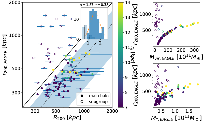
Figure 1: Left panel: Comparison of $R_{200}$ for EAGLE halos calculated using the extrapolation method described in Section 2 with $r_{\rm 200,EAGLE}$ inferred by direct extraction from the simulation data. The error bars show the $90\%$ CI of the 300 realizations for each halo taking into account different stellar masses and projection angles. The effective radius $r_{e}$ is colour coded. Open circles mark subhalos or groups which cannot be considered isolated, whereas filled circles mark main halos. The solid line marks a 1:1 correspondence. The inset plot shows the distribution of the ratio $R_{200}/r_{\rm 200,EAGLE}$, including the equivalent Gaussian fit. For main halos only we get a mean ratio of $1.57\pm 0.38$, which is hence included in the scatter plot as a dotted line and shaded area. Adding subgroups would give a mean ratio of $1.33\pm 0.54$. The histogram for the subhalos is highlighted by contoured semi-transparent bars. Top right panel: Comparison of $r_{\rm 200,EAGLE}$ with $M_{\rm vir}$ from the EAGLE simulation. Bottom right panel: as in the top panel but for stellar mass instead.

This Letter reports, from a study of 18 well-characterised strong lensing galaxies and 92 comparable simulated dark-matter halos, that the well-known concentration virial-mass relation for clusters appears to extend down to galaxy masses. However, the concentrations obtained are substantially higher than those predicted from numerical simulations. For instance, at a virial mass of $10^{12}\rm M_{\odot}$, the derived concentration is $c\sim 50$, whereas the simulations suggest $c\sim 10$ (Macciò et al., 2007). The discrepancy is statistically larger than the expected scatter found in the simulations. It could be expected from a systematic from the standard methodology applied to lensing data or from a sample selection bias (Sereno et al., 2015). However, it could also reflect differences in the assembly history of the targeted galaxies (Wang et al., 2020), although current simulations would struggle to produce halos with $c\sim 50$. There are indications of this conundrum already in earlier work (see Figure 4 in Leier et al., 2012), but without the control sample of simulated halos, these results could not exclude the possibility that the analysis and fitting method somehow biased the inferred concentrations. By assessing the methodology with a control sample, namely numerical simulations, we show in this letter that this result is robust, and warrants further investigation. Note that we use henceforth capital $R$ for projected 2D radii and lower case $r$ for 3D radii. Unless otherwise noted we give quantities based on the virial radius, which is the radius at which the mean enclosed density equals a certain multiple $\Delta_{c}$ (not necessarily 200) of the critical density following the definition in Bryan & Norman (1998).

2 Methodology

In this section, we briefly describe the methodology, laid out in more detail in Leier et al. (2012); Leier et al. (2016), that combines the lensing and stellar mass estimates to fit the density profile of the dark matter halo.

We start with the lensing mass maps provided by PixeLens (Saha & Williams, 2004). These were obtained by identifying point-like features in the lensed images, and solving the lensing equations for each system, producing a pixellated version of the surface mass density on the lens plane. The essence of PixeLens is to provide a large number of mass distributions in a non-parametric way that are compatible with the lens information, under a number of assumptions, enforced to produce realistic solutions. In order to assess uncertainties, we take 300 such maps from PixeLens. The extended lensed images are not fitted, which increases the uncertainty somewhat, but the difference is expected to be small (cf. Denzel et al., 2021). The stellar mass maps are produced by comparing the observed photometry with population synthesis models, following the same pixellated grid on the lens plane.

For each lens, we generate an ensemble of $\sim$$10^{4}$ dark matter mass maps, by subtracting a random member of the stellar map ensemble ($M_{*}$) from a random member of the lensing (i.e. total) mass ensemble ($M_{L}$). In this Monte Carlo procedure, we make sure unphysical cases – namely those that produce negative dark matter mass – are rejected. Therefore, a profile with low $M_{L}$ at small radius can only be combined with low $M_{*}$ values. This is an additional constraint not considered in our previous analysis presented in Leier et al. (2016). We then fit each dark matter map with a spherically symmetric NFW profile, projected on the lens plane, from which we extract the concentration ($c$) and virial mass ($\rm M_{\rm vir}$).

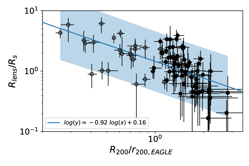
Figure 2: Comparing $R_{lens}/R_{s}$ with $R_{200}/r_{\rm 200,EAGLE}$ we find that the larger the reconstruction radius of the lens with respect to the NFW scale radius the lower the virial radius of our reconstruction method w.r.t. the $r_{\rm 200,EAGLE}$ taken directly from the EAGLE simulation. The blue area shows the $95\%$ confidence band. As in Fig. 1, we mark main halos (sub halos) with filled (open) circles.

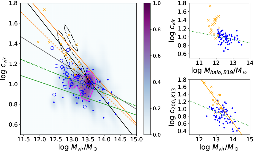
Figure 3: Left panel: Concentration vs virial mass plot shown with colour coded kernel densities. The solid magenta line shows the $68\%$ density contour in a kernel density estimation of the probability distribution for the EAGLE halos with an $\rm RMSD<0.06$ corresponding to the median of all RMSD values. The dashed black contours show the equivalent for the observed sample of lenses. The blue dots (open circles) show the median values of c_vir and M_vir of main halos (subhalos) in the EAGLE sample. The orange marks show the sample of observed lenses. The solid grey, black and green lines are the c-$\rm M_{\rm vir}$ relations of the X-ray selected sample of Buote et al. (2007), our previous best fit (Leier et al., 2016) and the simulation-based relation of Macciò et al. (2007), respectively. The green dashed line is the best fit to the EAGLE main halo data and the orange solid and dashed lines are the best fits to the complete lens sample and the RMSD selected (RMSD < 0.06) sample, i.e. lens_<50. Top right panel: as in the left panel but with a virial mass inferred by the stellar-to-halo mass relation of Behroozi et al. (2019). The green dotted line shows the fit to the EAGLE sample. No significant linear regression to the lens sample was found. Bottom right panel: as in the left panel but with a concentration based on the galaxy size-$\rm r_{\rm vir}$ relation of Kravtsov (2013).

In addition to the 18 lensing systems presented in Leier et al. (2016), we explore a set of 92 dark matter halos, selected from the EAGLE simulation (Schaye et al., 2015). The identical methodology is applied to these simulated data, to assess potential biases in the derivation of halo concentration. The EAGLE data are taken from the $z=0.1$ snapshot of the fiducial simulation RefL0100N1504. We extract the 3D positional information of the stellar, gas and dark matter particles considered as part of a given halo. We select all halos with galaxies more massive than $10^{10.75}\rm M_{\odot}$ in stellar mass. To account for halo-to-halo variance, we produce multiple projections of the simulated halos onto the lens plane by performing 100 random Euler rotations. The pixel size, Einstein radius and critical mass corresponding to each set is taken from the observed sample of 18 lenses. Therefore, the EAGLE sample represents a set with the same properties as the observed lenses, to remove any sample selection bias. Note that, by construction, the simulation data samples the enclosed mass profile at a radial range comparable with the observed lenses. Combined density contours weighted by the goodness of fit of each system – making use of the root mean square deviation, (hereafter $RMSD$), and the $\chi^{2}$ statistic – are then calculated for the lensing and the simulation data, respectively.

Table 1: Overview of the $c-\rm M_{\rm vir}$ power-law parameters according to Eq. 1. In col. 1, B07 refers to the results of Buote et al. (2007), M07 to Macciò et al. (2007) and L12 to Leier et al. (2012). The samples “lens” and “EAGLE” give the best fits from this paper. If we consider fits to our lens sample with a root mean square devation better than the median value – corresponding to the data the densities in Fig. 3 are based on – we obtain the results labeled “lens_<50”. Col. 2 is the slope of the scaling relation, col. 3 is the concentration of the best fit at virial mass $10^{14}$M_⊙ and col. 4 is the concentration at galaxy-scale dark matter halos ($10^{12}$M_⊙), the latter shown to illustrate the substantially higher concentration of halos in gravitational lensing galaxies. We provide errors from bootstrap. See Section 3 for sample details. Note that for lens sample “$B19$” no significant fit can be determined. Hence we provide the median concentration.

	Sample	$\alpha$	$c_{14}$	$c_{12}$
	(1)	(2)	(3)	(4)
lit.	B07	$-0.199\pm 0.026$	$9.12\pm 0.43$	$22.80\pm 1.08$
	L12	$-0.401\pm 0.064$	$7.03\pm 1.49$	$44.56\pm 9.44$
	M07	$-0.109\pm 0.005$	$6.34\pm 0.26$	$10.47\pm 0.43$
lens	$all$	$-0.65\pm 0.10$	$3.26^{+1.24}_{-0.90}$	$65.25^{+7.63}_{-8.64}$
	$<50$	$-0.41\pm 0.07$	$6.51^{+1.16}_{-1.41}$	$43.19^{+5.60}_{-6.43}$
	${B19}$	$-$	$-$	$19.43^{+10.24}_{-6.70}$
	${K13}$	$-0.62\pm 0.14$	$4.18^{+1.29}_{-1.86}$	$73.91^{+17.50}_{-22.93}$
EAGLE	$all$	$-0.13\pm 0.03$	$8.17^{+0.34}_{-0.36}$	$14.58^{+1.10}_{-1.19}$
	${ISO}$	$-0.08\pm 0.03$	$8.38^{+0.35}_{-0.36}$	$12.26^{+1.12}_{-1.23}$
	${B19}$	$-0.08\pm 0.04$	$7.23^{+0.81}_{-0.91}$	$10.43^{+0.31}_{-0.32}$
	${K13}$	$-0.19\pm 0.05$	$5.28^{+0.37}_{-0.39}$	$12.86^{+0.47}_{-0.49}$

Extrapolating the density profile estimate to a certain radius based on a fit to just a few supporting points at small radii comes along with uncertainties, which we are able to determine by means of the EAGLE halos. An underestimate of $R_{200}$, i.e. the radius for which the halo density equals 200 times the critical density, with respect to the actual value, is expected in cases where the fitting points are not sensitive to the scale radius $R_{s}$. To demonstrate the validity of the extrapolation to the virial radius, $R_{vir}$, and $R_{200}$ respectively, we compare in Fig. 1 the EAGLE values of $R_{200}$ with those derived independently, following our methodology. Note that the uncertainties on the ordinate, i.e. $r_{\rm 200,EAGLE}$, are not shown to avoid crowding, but are similar to those of our estimates of R₂₀₀ (abscissa). Fig. 1 shows that the $R_{200}$ values derived by the above method differ on average by $57\%$ from the original EAGLE values ($r_{200,EAGLE}$) with the 1:1 correspondence (solid line) lying $\sim 1.5\sigma$ apart if we consider main halos (filled circles) only. Subhalos (open circles) tend to have systematically larger EAGLE values. We like to point out that if our objects resemble more closely a subgroup environment rather than main halo environments a 1:1 relationship would fall well within $1\sigma$. After all a one-to-one mapping of our lens environments to given definitions of main halos versus subgroups from simulations might be an oversimplification, noting that subhalos themselves may be acting as lenses. However, for the main halos, a clear correlation between $R_{200}$ and $r_{200,EAGLE}$ is evident. The right top and bottom panels highlight the influence of the environment on $r_{\rm 200,EAGLE}$ and enclosed stellar and virial mass. By analysing the mass enclosed in the range between $r_{\rm 200,EAGLE}$ and the virial radius for the main halos, i.e. $\rm M_{\rm vir}-M_{200,EAGLE}$, a quantity that should be sensitive to the mass density in the environment, we find that there is no significant trend with $R_{200}$, $r_{\rm 200,EAGLE}$ or the stellar mass. The small scatter for main halos in the top and bottom panel indicates that EAGLE halos behave largely like the halos in abundance matching relations, stellar-to-halo mass as well as size-$R_{vir}$ relations, which will be further analysed in Section 3. More importantly, the uncertainties of $\sim 57\%$ (for main halos only) or $\sim 33\%$ (for main halos and subgroups) do not explain (a) the large offset between the concentrations found in the observed lenses and the EAGLE halos, and (b) the increasing offset towards lower $\rm M_{\rm vir}$. There is however a significant inverse trend of $R_{200}/r_{200,EAGLE}$ with $R_{lens}/R_{s}$ shown in Fig. 2 where $R_{s}$ denotes the NFW scale radius. This implies that our extrapolation will be closer to the actual values if the reconstructed portion of the lens is large enough to be sensitive to the radius where the dark matter density profile turns over to a $r^{-3}$ dependence. However, balancing this effect by dividing $R_{200}$ by 1.57 for main halos only (1.33 for main halos and subgroups) leads to roughly a $36\%$ ($25\%$) decrease in concentration, which is not enough to reconcile the lensing galaxies with total mass below $10^{13}M_{\odot}$ with simulations.

There seems to be no obvious correlation with the distribution of stellar matter as shown by the colour coded effective radii in Fig. 1. Note that we compute the $90\%$ C.I. uncertainties of $R_{200}$ by using 100 different projection angles. The uncertainties of $r_{200,EAGLE}$ (i.e. on the vertical axis) are roughly of the same extent as they describe halo properties such as ellipticity and environment. We omit them to avoid crowding in the plot. In a follow-up study (in preparation) we systematically explore the dependency of the $c$-$\rm M_{\rm vir}$ relation on additional factors such as the slope of a generalized NFW dark matter profile, the slope of the IMF, additional matter components as well as variations of the original lens profiles, to assess various ways of reconciling observed and simulated data.

3 Contrasting lens and EAGLE data

A comparison of the sample of 18 observed lenses along with 92 simulated halos from EAGLE is shown in Fig. 3. The lenses cover a range in terms of lens mass, i.e. roughly the total mass enclosed within the Einstein radius, of $(0.06-0.45)\times 10^{12}\rm M_{\odot}$ and according to our extrapolation up to $R_{vir}$, the sample corresponds to a virial mass range of $(0.32-17.8)\times 10^{12}\rm M_{\odot}$. The orange crosses represent the observed lenses, whereas the blue marks correspond to the EAGLE halos. 67 of which are rather isolated main halos (blue dots), the remaining 25 belong to halo subgroups (open circles). Further key parameters of the lenses can be found in Table 2 below and Table 1 and 3 of Leier et al. (2016). In order to balance the differing number of valid fits (goodness of fit is evaluated here using $RMSD$, defined above), and MC realisations, we pick the same number of $(c,\rm M_{\rm vir})$-points from every lens and halo with a $RMSD<0.06$, which corresponds to the median of all $RMSD$ values, to obtain the orange dashed line in Fig. 3. Fitting parameters to the latter sample, labeled “${\rm lens}_{<50}$”, are provided in Table 1. A fit to all $(c,\rm M_{\rm vir})$-points, i.e. unfiltered with respect to $RMSD$, results in the orange solid line and the parameters labeled “lens” in Table 1. We furthermore fix the IMF to Salpeter, although we note that the choice of a lighter IMF, such as Chabrier, does not change the results. A comparison of “lens” with “lens_<50” shows that even the introduced $RMSD$ selection does not reconcile the $c-\rm M_{\rm vir}$ relation with results from numerical simulations. We find that the new analysis of the concentration - virial mass relation for the observed lens sample is hence in good agreement with the fit proposed by Leier et al. (2012, solid black line). Moreover, a subsample with the best fit results gives a concentration at Milky-Way sized halos of c${}_{12}\sim 40\pm 5$, in stark contrast with the lower concentrations found in the EAGLE simulations, c${}_{12}\sim 15\pm 1$. Furthermore, the EAGLE halos – studied in exactly the same way, using the same pixelisation as the observational sample – follow a significantly shallower $c-\rm M_{\rm vir}$ relation (green dashed line). Note that applying the balancing factor of $R_{200}/r_{200,EAGLE}$ ($1.33$ for main and subgroups) from the previous section to both lens and EAGLE sample concentrations, will change c₁₂ to $30$ for the lens sample and $\sim 11$ for the EAGLE sample. Also the virial masses will change by a factor of $\sim 2.3$ towards lower values, but still keeping the two c-M relations significantly apart. This is also true if we compare the distributions of concentrations instead of the normalisation c₁₂. For the given lens sample we obtain a median concentration of $19.9_{-9.1}^{+14.2}$ versus $9.8_{-3.3}^{+4.0}$ for the EAGLE sample. Applying the above corrections will certainly bring the two populations closer together, but leaves the populations incompatible within their $90\%$ C.I. In Tab. 1 we give the fit parameters for the whole EAGLE sample (’all’) and for isolated main halos only (’ISO’). Both fits agree, however, within their uncertainties. The concentration of the simulated halos mostly fall below the $c-\rm M_{\rm vir}$ relation found by Buote et al. (2007) (grey) and the one of Leier et al. (2012) (black) – a finding consistent with other $c-\rm M_{\rm vir}$ relations from simulations. We include the one from Macciò et al. (2007) as a solid green line in Fig. 3, and list results of observational and numerical studies alike in Table 1. Note that the offset between the EAGLE and the Macciò et al. (2007) scaling relations, both based on numerical simulations, can be explained by the different redshift of the sample, following Eq. 1. However, the slopes are in good agreement. The results are put into context of known relations from abundance matching. We use the stellar-to-halo mass relation by Behroozi et al. (2019, B19, top right panel in Fig. 3), and the galaxy size-virial radius relation by Kravtsov (2013, K13, bottom right panel), and find that, despite a certain shift of 0.3-0.5 dex in halo mass for B19, a rather small average shift of 0.1 going from $\log{c_{vir}}$ to $\log{c_{200}}$ for K13 and a slightly increased scatter, the mismatch between lens and EAGLE c-M fits remains. We like to point out that an offset of $\sim+0.3$ dex is already present when comparing EAGLE halo masses with their respective halo masses according to B19. Using a sample of EAGLE main halos raises the question whether the lens sample is systematically different with respect to its environment. Based on an extensive discussion in Section 3.1 of Leier et al. (2016), we conclude that half of the lenses reside in cluster or group surroundings which they dominate, and the other half has only isolated companions, if any. Thus, no striking contrast is noticeable when comparing the lens and the EAGLE sample.

4 Conclusions

This letter focuses on the concentration vs virial mass relation of dark matter halos derived from strong lensing data, extending the results of Leier et al. (2012) by a more robust model fitting methodology, and, most importantly, contrasting the results from the observed data with synthetic systems extracted from the EAGLE cosmological hydrodynamical simulations, randomised to remove individual variations from halo to halo, from which we produce test mass maps in the same format as those used to explore the observed sample comprising 18 lenses from the CASTLES survey. The comparison with simulated data allows us to assess whether the high concentrations derived in Leier et al. (2012) are real, or rather, produced by the methodology.

On a concentration-virial mass diagram (Fig. 3) we find the observed halo parameters to be consistent with previous results from lensing studies and in agreement with X-ray observations within uncertainties. Furthermore, we show that the difference between the $c-\rm M_{\rm vir}$ relations from numerical simulations and lensing results cannot be explained by methodological differences as we are able to recover the shallower slope of the scaling relation known for simulations while applying the same method to EAGLE halos. Therefore, we conclude that the high concentrations found in dark matter halos at virial mass $\sim 10^{12}\rm M_{\odot}$ are not accounted for in state-of-the-art numerical simulations (e.g. Correa et al., 2015; Chua et al., 2019). Baryonic processes can lead to the contraction of the dark matter halo (Blumenthal et al., 1986; Gnedin et al., 2004), although the net effect is in question, and an opposite evolution (i.e. halo expansion) can ensue due to feedback (Dutton et al., 2016). Leier et al. (2012) already showed that simple adiabatic contraction models cannot account for the mismatch in concentration at lower halo mass. The analysis of Chua et al. (2019) on Illustris halos shows that the (log) concentration can shift by $\sim+$0.25 dex, when comparing their full simulations – including baryon processes – with dark-matter only halos. Our results suggest that simulated halos with baryon physics taken into account, are nevertheless underestimating the (log) concentration by as much as $\sim+$0.6 dex in $\sim 10^{12}\rm M_{\odot}$ halos. Even if abundance matching is taken at face value, the discrepancy is still $\sim+$0.3 dex.

The study presented here is part of a series of research efforts that investigate physical processes and methodological peculiarities such as sampling biases that may cause the incompatibility of observations and simulations especially in the low mass range of Early Type Galaxies. In another paper (Leier et al., in prep.), we will explore in more detail the bias aspect and peculiarities of the dark matter profiles of lensing galaxies.

Table 2: Overview of the lens sample: morphology, scale radius $R_{s}$, virial radius $R_{vir}$, concentration $c_{vir}$ and mass $M_{vir}$ as shown in Fig. 3 all with $68\%$ CI. For further lens properties such as stellar mass we refer to Table 3 in Leier et al. (2016). For J1402 and J1719 the probed region of the halos do not constrain the NFW fit by much. Because of this we get many equally good fits. Consequently, introducing a selection based on the median RMSD (see the definition of $lens_{<50}$ in Section 3) does not help in our effort to narrow down the uncertainties.

Lens ID	Morph.	$R_{s}$	$R_{vir}$	$c_{vir}$	$M_{vir}$
		[kpc]	[kpc]		[$10^{12}\rm M_{\odot}$]
J0037-0942	E	$40.6_{-26.8}^{+43.0}$	$454.57_{-118.7}^{+165.0}$	$11.7_{-4.7}^{+13.0}$	$8.1_{-4.8}^{+12.0}$
J0044+0113	E	$15.3_{-3.8}^{+6.0}$	$473.1_{-52.1}^{+64.0}$	$30.5_{-5.1}^{+6.0}$	$8.0_{-2.4}^{+4.0}$
J0946+1006	E	$20.3_{-5.9}^{+10.0}$	$413.0_{-34.3}^{+52.0}$	$20.4_{-5.1}^{+6.0}$	$6.3_{-1.5}^{+3.0}$
J0955+0101	S	$37.2_{-22.7}^{+12.0}$	$607.3_{-193.1}^{+74.0}$	$16.6_{-2.7}^{+12.0}$	$16.6_{-11.3}^{+7.0}$
J0959+0410	E	$19.7_{-11.5}^{+20.0}$	$423.2_{-131.5}^{+136.0}$	$21.7_{-7.7}^{+14.0}$	$5.8_{-3.9}^{+8.0}$
J1100+5329	E	$60.82_{-43.10}^{+30.0}$	$562.7_{-211.7}^{+76.0}$	$9.3_{-2.2}^{+11.0}$	$18.8_{-14.2}^{+9.0}$
J1143-0144	E	$23.8_{-12.6}^{+15.0}$	$573.8_{-167.7}^{+110.0}$	$24.5_{-6.8}^{+12.0}$	$13.9_{-8.9}^{+10.0}$
J1204+0358	E	$15.9_{-8.7}^{+19.0}$	$383.8_{-102.1}^{+133.0}$	$24.8_{-9.5}^{+16.0}$	$4.6_{-2.8}^{+7.0}$
J1213+6708	E	$22.9_{-15.1}^{+28.0}$	$440.0_{-151.1}^{+177.0}$	$19.4_{-7.7}^{+19.0}$	$6.4_{-4.6}^{+11.0}$
J1402+6321	E	$4.3_{-4.1}^{+16.0}$	$252.4_{-66.8}^{+144.0}$	$54.3_{-36.3}^{+72.0}$	$1.4_{-0.8}^{+4.0}$
J1525+3327	E	$51.6_{-25.0}^{+13.0}$	$539.3_{-85.3}^{+63.0}$	$11.1_{-2.2}^{+6.0}$	$17.7_{-7.1}^{+7.0}$
J1531-0105	E	$36.0_{-16.4}^{+30.0}$	$519.7_{-104.7}^{+144.0}$	$14.1_{-4.3}^{+6.0}$	$11.3_{-5.6}^{+12.0}$
J1538+5817	E	$8.70_{-8.3}^{+36.0}$	$225.55_{-93.3}^{+211.0}$	$25.9_{-17.6}^{+272.0}$	$0.9_{-0.7}^{+6.0}$
J1630+4520	E	$41.8_{-17.9}^{+23.0}$	$509.1_{-58.1}^{+118.0}$	$12.2_{-3.2}^{+6.0}$	$12.4_{-3.8}^{+11.0}$
J1719+2939	E/S0	$11.6_{-9.1}^{+32.0}$	$286.7_{-101.8}^{+185.0}$	$25.8_{-15.5}^{+51.0}$	$2.0_{-1.4}^{+7.0}$
J2303+1422	E	$27.5_{-13.5}^{+30.0}$	$478.2_{-123.4}^{+145.0}$	$17.81_{-6.6}^{+9.0}$	$8.8_{-5.2}^{+11.0}$
J2343-0030	E/S0	$14.2_{-8.1}^{+23.0}$	$394.5_{-100.2}^{+174.0}$	$28.6_{-13.1}^{+22.0}$	$5.1_{-3.0}^{+10.0}$
J2347-0005	E	$33.7_{-12.2}^{+18.0}$	$518.8_{-120.6}^{+70.0}$	$15.4_{-4.5}^{+4.0}$	$17.4_{-9.5}^{+8.0}$

Data Availability

This sample is extracted from publicly available data from the CASTLES sample (Falco et al., 2001) and the EAGLE simulations (Schaye et al., 2015). The combined final dataset is available upon reasonable request.

References

- Behroozi et al. (2019) Behroozi P., Wechsler R. H., Hearin A. P., Conroy C., 2019, Monthly Notices of the Royal Astronomical Society, 488, 3143–3194
- Biviano et al. (2017) Biviano A., et al., 2017, A&A, 607, A81
- Blumenthal et al. (1986) Blumenthal G. R., Faber S. M., Flores R., Primack J. R., 1986, ApJ, 301, 27
- Bryan & Norman (1998) Bryan G. L., Norman M. L., 1998, The Astrophysical Journal, 495, 80–99
- Buote et al. (2007) Buote D. A., Gastaldello F., Humphrey P. J., Zappacosta L., Bullock J. S., Brighenti F., Mathews W. G., 2007, The Astrophysical Journal, 664, 123–134
- Chua et al. (2019) Chua K. T. E., Pillepich A., Vogelsberger M., Hernquist L., 2019, MNRAS, 484, 476
- Comerford & Natarajan (2007) Comerford J. M., Natarajan P., 2007, Monthly Notices of the Royal Astronomical Society, 379, 190–200
- Correa et al. (2015) Correa C. A., Wyithe J. S. B., Schaye J., Duffy A. R., 2015, MNRAS, 452, 1217
- Denzel et al. (2021) Denzel P., Coles J. P., Saha P., Williams L. L. R., 2021, MNRAS, 501, 784
- Diemer & Kravtsov (2015) Diemer B., Kravtsov A. V., 2015, ApJ, 799, 108
- Dutton & Macciò (2014) Dutton A. A., Macciò A. V., 2014, MNRAS, 441, 3359
- Dutton et al. (2016) Dutton A. A., et al., 2016, MNRAS, 461, 2658
- Ettori et al. (2010) Ettori S., Gastaldello F., Leccardi A., Molendi S., Rossetti M., Buote D., Meneghetti M., 2010, A&A, 524, A68
- Falco et al. (2001) Falco E. E., et al., 2001, in Brainerd T. G., Kochanek C. S., eds, Astronomical Society of the Pacific Conference Series Vol. 237, Gravitational Lensing: Recent Progress and Future Go. p. 25
- Gnedin et al. (2004) Gnedin O. Y., Kravtsov A. V., Klypin A. A., Nagai D., 2004, ApJ, 616, 16
- Klypin et al. (2016) Klypin A., Yepes G., Gottlöber S., Prada F., Heß S., 2016, MNRAS, 457, 4340
- Kravtsov (2013) Kravtsov A. V., 2013, The Astrophysical Journal, 764, L31
- Leier et al. (2011) Leier D., Ferreras I., Saha P., Falco E. E., 2011, ApJ, 740, 97
- Leier et al. (2012) Leier D., Ferreras I., Saha P., 2012, Monthly Notices of the Royal Astronomical Society, 424, 104–114
- Leier et al. (2016) Leier D., Ferreras I., Saha P., Charlot S., Bruzual G., La Barbera F., 2016, Monthly Notices of the Royal Astronomical Society, 459, 3677–3692
- Macciò et al. (2007) Macciò A. V., Dutton A. A., Van Den Bosch F. C., Moore B., Potter D., Stadel J., 2007, Monthly Notices of the Royal Astronomical Society, 378, 55–71
- Mandelbaum et al. (2008) Mandelbaum R., Seljak U., Hirata C. M., 2008, J. Cosmology Astropart. Phys., 2008, 006
- Martinsson et al. (2013) Martinsson T. P. K., Verheijen M. A. W., Westfall K. B., Bershady M. A., Andersen D. R., Swaters R. A., 2013, A&A, 557, A131
- Merten et al. (2015) Merten J., et al., 2015, ApJ, 806, 4
- Navarro et al. (1997) Navarro J. F., Frenk C. S., White S. D. M., 1997, ApJ, 490, 493
- Prada et al. (2012) Prada F., Klypin A. A., Cuesta A. J., Betancort-Rijo J. E., Primack J., 2012, MNRAS, 423, 3018
- Saha & Williams (2004) Saha P., Williams L. L. R., 2004, AJ, 127, 2604
- Schaye et al. (2015) Schaye J., et al., 2015, MNRAS, 446, 521
- Sereno et al. (2015) Sereno M., Giocoli C., Ettori S., Moscardini L., 2015, MNRAS, 449, 2024
- Shan et al. (2017) Shan H., et al., 2017, ApJ, 840, 104
- Walker & Peñarrubia (2011) Walker M. G., Peñarrubia J., 2011, ApJ, 742, 20
- Wang et al. (2020) Wang K., Mao Y.-Y., Zentner A. R., Lange J. U., van den Bosch F. C., Wechsler R. H., 2020, MNRAS, 498, 4450