New Physics Through Drell Yan SMEFT Measurements at NLO

Abstract

Drell Yan production is a sensitive probe of new physics and as such has been calculated to high order in both the electroweak and QCD sectors of the Standard Model, allowing for precision comparisons between theory and data. Here we extend these calculations to the Standard Model Effective Field Theory (SMEFT) and present the NLO QCD and electroweak contributions to the neutral Drell Yan process.

I Introduction

The measurement of the neutral Drell-Yan (DY) process, $pp\rightarrow Z^{*},\gamma^{*}\rightarrow l^{+}l^{-}$, has provided important validation of Standard Model (SM) predictions, has served as a testing ground for searches for high mass $Z^{\prime}$ bosons and other new physics scenarios, and most recently as a probe of deviations from the SM in an effective field theory context. For all of these applications, precise theoretical predictions both in the SM and in the effective field theory are crucial.

The SM results for the neutral DY process, along with NLO QCDAltarelli:1979ub ; KubarAndre:1978uy and NLO electroweakBaur:2001ze ; Dittmaier:2001ay corrections were derived many years ago. QCD results at NNLOHamberg:1990np ; Anastasiou:2003yy ; Anastasiou:2003ds ; Melnikov_2006 ; Catani:2009sm ; Li:2012wna ; Camarda:2019zyx are known for both the total cross section and for some differential distributions. Further QCD results exist to N³LL+NNLO and to N³LODuhr:2020seh ; Duhr:2020sdp ; Becher:2020ugp ; Re:2021con ; Bizo_2018 . The combined NNLO QCD and NLO electroweak (EW) corrections to high mass DY pairs have been studied in detailKilgore:2011pa ; Buccioni:2020cfi ; Delto:2019ewv ; Boughezal:2013cwa ; Buonocore:2019puv ; Dittmaier:2020vra ; Bonciani:2020tvf ; Heller:2020owb . The state of the art DY predictions are in excellent agreement with experimental resultsatlascollaboration2020measurement ; Sirunyan:2018owv suggesting that possible new physics affecting DY production is either at a very high energy scale or is extremely weakly coupled such that current experiments are only weakly sensitive to these effects. In the effective field theory context, the new physics effects can show up as enhancements at large partonic energy scales, where the effects of electroweak Sudakov logarithms are relatively largeDenner_2001 ; Campbell:2016dks , mandating precision calculations in the effective field theory beyond the existing SM results.

Without the discovery of new high mass particles, the search for beyond the standard model (BSM) physics can be pursued using an effective field theory. The SM effective field theory (SMEFT)Brivio:2017vri assumes that the Higgs particle is contained in an $SU(2)_{L}$ doublet and that weak scale interactions can be described by the Lagrangian,

$$L\sim L_{SM}+\Sigma_{i,n}{C_{i}^{n}\over\Lambda^{n-4}}O_{i}^{n}\,,$$ (1)

where the operators $O_{i}^{n}$ have dimension-$n$ and contain only SM particles and $\Lambda$ parameterizes the ultraviolet (UV) cut-off scale. BSM physics is then described by non-zero values of the coefficient functions $C_{i}^{n}$. Since the operators have dimension greater than $4$, they typically generate effects that grow with energy and can be searched for in the tails of distributions.

There has been considerable progress in the development of simulation tools for the SMEFTBrivio:2020onw ; Degrande:2020evl . At present, the SMEFT dimension-6 operators can be included at NLO QCD using these tools. There are also numerous specialized studies of individual processes that include NLO QCDBaglio:2020oqu ; Baglio:2019uty ; Baglio:2018bkm ; Alioli:2018ljm . The NLO electroweak (EW) corrections, however, are currently performed on a case by case basis. Most of the NLO EW studies involve decays: $H\rightarrow b{\overline{b}}$Cullen:2020zof ; Cullen:2019nnr ; Gauld:2016kuu , $H\rightarrow\gamma\gamma$Hartmann_2015 ; Hartmann_2015x ; Dawson:2018liq ; Dedes:2018seb , $H\rightarrow ZZ^{*}$Dawson:2018pyl , $H\rightarrow Z\gamma$Dawson:2018pyl ; Dedes:2019bew , $H\rightarrow WW^{*}$Dawson:2018liq , $Z\rightarrow f{\overline{f}}$Dawson:2019clf ; Hartmann:2016pil , and $t\rightarrow Wb$Boughezal:2019xpp . The only $2\rightarrow 2$ particle scattering process that has been studied at the NLO EW level is DY. Our previous DY studyDawson:2018dxp concentrated on the effect of a single operator, while the current study represents the first NLO EW study of a $2\rightarrow 2$ process that includes the effects of multiple operators.

At tree level in the dimension-6 truncation of the SMEFT, the DY process depends on operators that affect the input parameter relationships and on 4-fermion operators that can dominate the rate at high energy and distort the shapes of kinematic distributionsPanico:2021vav ; Torre:2020aiz ; deBlas:2013qqa . The $Z$ pole resonance contributions to lepton pair production at NLO QCD and NLO EW in the SMEFT similarly involve many additional coefficients beyond those occurring at tree levelDawson:2019clf . In this work, we extend our previous DY calculationDawson:2018dxp to include the complete set of SMEFT bosonic operatorsWells:2015uba that contribute at NLO QCD and EW to the process, $q{\overline{q}}\rightarrow\gamma^{*},Z^{*}\rightarrow l^{+}l^{-}$. Our results are of particular interest in the low energy limit of UV models that do not generate $4$-fermion operators at tree level. This interesting class of models includes models with $SU(2)$ scalar singlets, doublets and triplets, as well as models with vector-like fermionsdeBlas:2017xtg . If $4-$fermion operators arise at tree level (as is the case in models with a heavy $Z^{\prime}$ boson), the tree level SMEFT effects from these operators will likely dominate over the NLO EW loop effects. We are therefore motivated by the case where $4-$ fermion operators are not generated at the UV scale and where the NLO EW effects may play a significant role in low energy DY phenomenology. We emphasize, however, that our results are independent of model assumptions and represent an important step in the NLO EW SMEFT program.

In Sect. II, we review the SMEFT formalism relevant for this study, along with the lowest order SMEFT result for the DY process. Sect. III contains the details of our SMEFT calculation and our results are summarized in Sect. IV. Our complete analytic result is attached as supplemental material which can be included in existing Monte Carlo programs.

II SMEFT basics

The SMEFT Lagrangian contains an infinite tower of $SU(3)\times SU(2)_{L}\times U(1)_{Y}$ invariant operators constructed from SM fields. In this work, we restrict ourselves to the dimension -6 operators, assume all coefficients are real and do not consider the effects of CP violation. We use the Warsaw basis Buchmuller:1985jz ; Grzadkowski:2010es and normalize the coefficients as in Eq. 1. We include flavor indices on our results and compute amplitudes to linear order in the dimension-6 SMEFT coefficients and at 1-loop in the QCD and electroweak couplings. The electroweak sector is described by three input parameters which we take to be $M_{W},M_{Z}$ and $G_{\mu}$, while the electromagnetic coupling, $\alpha$, is a derived quantity. We define $w=M_{W}^{2}$, $z=M_{Z}^{2}$ and $v$ to be the $(VEV)^{2}$ of the Higgs field.

The input parameters are related to the gauge couplings ${\overline{g}}_{1}$ and ${\overline{g}}_{2}$ in the Lagrangian to ${\cal{O}}\biggl{(}{1\over\Lambda^{2}}\biggr{)}$ as, Dedes:2017zog ; Alonso:2013hga ; Brivio:2017bnu

$$w = {{\overline{g}_{2}^{2}}v\over 4}$$

$$z = \frac{({\overline{g}}_{1}^{2}+{\overline{g}}_{2}^{2})v}{4}+\frac{v^{2}}{\Lambda^{2}}\left(\frac{1}{8}({\overline{g}}_{1}^{2}+{\overline{g}}_{2}^{2})C_{\phi D}+\frac{1}{2}{\overline{g}}_{1}{\overline{g}}_{2}C_{\phi WB}\right).$$ (2)

Dimension-6 4-fermion operators give contributions to the decay of the $\mu$, changing the relation between the vev-squared, $v$, and $G_{\mu}$,

$$G_{\mu}\equiv\frac{1}{\sqrt{2}v}-\frac{1}{2\sqrt{2}\Lambda^{2}}\biggl{(}C_{ll,2112}+C_{ll,1221}\biggr{)}+{\sqrt{2}\over 2\Lambda^{2}}\biggl{(}C_{\phi l,11}^{(3)}+C_{\phi l,22}^{(3)}\biggr{)}\,,$$ (3)

where the subscripts refer to the generation. When we perform our NLO calculations, $\sqrt{v}$ is always defined as the minimum of the potential, as in Ref. Degrassi:2014sxa .

In the dimension-$6$ truncation of the SMEFT, the amplitude for the DY process can be written to $1-$loop order as

$$A \sim A_{SM}+\Sigma_{i}{C_{i}^{6}\over\Lambda^{2}}A_{i,LO}^{6}+\Sigma_{j}{D_{j}^{6}\over 16\pi^{2}\Lambda^{2}}A_{j,NLO}^{6}\,,$$ (4)

where $A_{SM},A_{i,LO}^{6}$, and $A_{j,NLO}^{6}$ are the SM, dimension-$6$ tree level, and dimension-$6$ $1-$ loop contributions, respectively. We define the linear SMEFT result as,

$$\mid A\mid^{2}_{lin} \equiv \mid A_{SM}\mid^{2}+2Re\biggl{(}\Sigma_{i}A_{SM}^{*}{C_{i}^{6}\over\Lambda^{2}}A_{i,LO}^{6}\biggr{)}$$ (5)

$$+2Re\biggl{(}\Sigma_{i}A_{SM}^{*}{D_{i}^{6}\over 16\pi^{2}\Lambda^{2}}A_{j,NLO}^{6}\biggr{)}\,.$$

We note that Eq. 5 is not positive definite. For our purposes, we define the quadratic SMEFT result as

$$\mid A\mid^{2}_{quad} \equiv \mid A_{SM}+\Sigma_{i}{C_{i}^{6}\over\Lambda^{2}}A_{i,LO}^{6}+\Sigma_{j}{D_{j}^{6}\over 16\pi^{2}\Lambda^{2}}A_{j,NLO}^{6}\mid^{2}\,.$$ (6)

The quantity defined in Eq. 6 is what is typically used in SMEFT phenomenology studies and in global fits. There are, however, two types of “quadratic” ${\cal{O}}({1\over\Lambda^{4}})$ terms that are not included in Eq. 6. These are the interference of the dimension-$8$ operators with the SM resultBoughezal:2021tih ; Boughezal:2021tih and the double insertions of the dimension-$6$ operators in the amplitude that are beyond the scope of current NLO EW SMEFT calculations.

II.1 LO Drell Yan Results

We write the helicity amplitudes for $q(p_{1}){\overline{q}}(p_{2})\rightarrow l^{+}(p_{3})l^{-}(p_{4})$ in terms of the matrix elements,

$$M_{XY}=\biggl{[}{\overline{u}}(p_{2})\gamma_{\mu}P_{X}u(p_{1})\biggr{]}\cdot\biggl{[}{\overline{u}}(p_{3})\gamma^{\mu}P_{Y}u(p_{4})\ \biggr{]}\,,$$ (7)

with $P_{L,R}={1\mp\gamma_{5}\over 2}$. The tree level helicity amplitudes are,

$$A_{XY,LO}=G_{XY}M_{XY}$$ (8)

with

$$G_{XY}=G_{XY}^{SM}+\delta G_{XY}.$$ (9)

Summing over helicity amplitudes and averaging over the spin and color,

$$\mid{\overline{A}}_{LO}(s,t)\mid^{2} \equiv {1\over 12}\Sigma_{XY}\mid G_{XY}\mid^{2}\mid M_{XY}\mid^{2}$$ (10)

$$\equiv {1\over 12}\mid A_{LO}\mid^{2}\,.$$

The spin and color averaged partonic cross sections are,

$${d{\hat{\sigma}}\over dt} = {1\over 48\pi s^{2}}\biggl{\{}(\mid G_{LL}\mid^{2}+\mid G_{RR}\mid^{2})u^{2}+(\mid G_{LR}\mid^{2}+\mid G_{RL}\mid^{2})t^{2}\biggr{\}}$$

$${\hat{\sigma}}_{LO} = {1\over 16\pi s^{2}}\int_{-s}^{0}dt\mid{\overline{A}}_{LO}(s,t)\mid^{2}\,,$$ (11)

where $s=(p_{1}+p_{2})^{2},t=(p_{1}-p_{3})^{2}$ and $u=(p_{1}-p_{4})^{2}$.

The SM contribution is,

$$G_{LL}^{SM} = {4\sqrt{2}w(z-w)\over z}{G_{\mu}Q_{q}Q_{l}\over s}+{g_{L}^{q}g_{L}^{l}\over s-M_{Z}^{2}}$$

$$G_{LR}^{SM} = {4\sqrt{2}w(z-w)\over z}{G_{\mu}Q_{q}Q_{l}\over s}+{g_{L}^{q}g_{R}^{l}\over s-M_{Z}^{2}}$$

$$G_{RL}^{SM} = {4\sqrt{2}w(z-w)\over z}{G_{\mu}Q_{q}Q_{l}\over s}+{g_{R}^{q}g_{L}^{l}\over s-M_{Z}^{2}}$$

$$G_{RR}^{SM} = {4\sqrt{2}w(z-w)\over z}{G_{\mu}Q_{q}Q_{l}\over s}+{g_{R}^{q}g_{R}^{l}\over s-M_{Z}^{2}}\,.$$ (12)

with $g_{L}^{f}=\sqrt{\sqrt{2}G_{\mu}z}\biggl{[}\tau^{f}-2Q_{f}\biggl{(}1-{w\over z}\biggr{)}\biggr{]}$, $\tau^{f}=\pm 1$, $g_{R}^{f}=\sqrt{\sqrt{2}G_{\mu}z}\biggl{[}-2Q_{f}\biggl{(}1-{w\over z}\biggr{)}\biggr{]}$, and $Q_{f}$ is the fermion charge.

The tree level SMEFT contribution is given in Appendix A and depends on the coefficients,

$${\mathcal{C}_{\phi WB}},\,\mathcal{C}_{\phi D},\,\mathcal{C}_{\phi l,11}^{(3)},\,\mathcal{C}_{\phi l,22}^{(3)},\,\mathcal{C}_{\phi l,22}^{(1)},\mathcal{C}_{\phi e,22},\mathcal{C}_{\phi q,11}^{(3)},\,\mathcal{C}_{\phi q,11}^{(1)},\,\mathcal{C}_{\phi u,11},\,\mathcal{C}_{\phi d,11},\,$$

$$\biggl{[}\,\mathcal{C}_{ll,1221},\,\mathcal{C}_{ll,2112},\,\mathcal{C}_{lq,2211}^{(3)},\,\mathcal{C}_{lq,2211}^{(1)},\,\mathcal{C}_{qe,1122},\,\mathcal{C}_{lu,2211},\,\mathcal{C}_{ld,2211},\,\mathcal{C}_{ed,2211},\,\mathcal{C}_{eu,2211},\biggr{]}$$ (13)

The subscripts are generation indices, and the coefficients in the square brackets are 4-fermion operators. The numerical impact of the tree level $4-$fermion operators has been explored in many placesdeBlas:2013qqa ; Berthier:2015gja ; Carpentier:2010ue ; Falkowski:2017pss ; Cirigliano:2012ab . In this work, we will ignore the $4-$fermion contributions and focus instead in the impact of the sub-leading (in $s$) universal coefficients that involve the bosonic operators at $1-$loop. Our goal is to begin the exploration of the effects in Drell Yan production of operators that first arise at $1$-loop order. Typically, the $4-$fermion and bosonic operators occur in different types of UV theories. A complete classification of the quantum numbers of high scale particles that generate the various operators at tree level is given in Ref. deBlas:2017xtg . For example, models with UV scalars typically do not generate $4$-fermion operatorsDawson:2017vgm ; deBlas:2014mba , while a model with a sequential $Z^{\prime}$ gauge boson will generate such operatorsdeBlas:2017xtg that can be probed using kinematic observables in DY production Alioli:2017nzr ; Panico:2021vav .

It has been pointed out in Ref. Breso-Pla:2021qoe that due to the large Drell Yan cross section, information not from the high energy tail can potentially yield important information on SMEFT cross sections and so the coefficients of the dimension-$6$ operators could be significantly restricted by Drell Yan scattering, even at relatively low energies. In fact, the one-loop EW contributions to $Z$ decays in the SMEFT can be as large as ${\cal{O}}(10-20)\%$ at LHC energiesDawson:2019clf ; Dawson:2018jlg . Ref. Farina:2016rws computed a set of SMEFT contributions to the neutral DY process and found that the high luminosity LHC will have significant sensitivity to these effects. Here we extend that calculation to include the full set of SMEFT QCD and electroweak corrections from bosonic operators.

III NLO Calculation of Drell-Yan Production in the SMEFT

III.1 Virtual Contributions to NLO SMEFT Drell Yan Results

Figure 1: Sample Feynman diagrams contributing to the $1$-loop virtual contribution.

In this section we detail the calculation of the virtual NLO corrections to the Drell-Yan process in the SMEFT. We follow the notation ofDawson:2018pyl ; Dawson:2019clf ; Dawson:2018dxp ; Dawson:2018liq . The operators that appear in $1-$loop amplitudes are those in Eq. 13 together with

$$\mathcal{C}_{W},\,\mathcal{C}_{\phi\square},\,\mathcal{C}_{\phi W},\,\mathcal{C}_{\phi B},\,\mathcal{C}_{uW,33},\,\mathcal{C}_{uB,33},\,\mathcal{C}_{\phi l,aa}^{(3)},\,\mathcal{C}_{\phi l,aa}^{(1)},\mathcal{C}_{\phi e,aa},\mathcal{C}_{\phi q,aa}^{(3)},\,\mathcal{C}_{\phi q,aa}^{(1)},\,\mathcal{C}_{\phi u,aa},\,\mathcal{C}_{\phi d,aa},$$ (14)

where the subscript $aa=11,22,33$ is a generation index.

It is convenient to separate the contributions to the virtual NLO corrections into box contributions, vertex contributions, propagator contributions and the contributions from renormalization counterterms. These are shown schematically in Fig. 1. As we clarified in the introduction, we do not include $4$-fermion operators in our calculation, since we are interested in effects which first occur at $1-$loop. Furthermore, we calculate only the NLO corrections that interfere with the LO amplitudes. As a result of these restrictions, the only topologies that enter in our calculations are the ones already present at the SM level.

The virtual corrections to Drell Yan suffer from UV divergences, along with soft and collinear infrared (IR) divergences. We regularize the UV divergences by working in $d=4-2\epsilon$ dimensions, while the IR divergences are regularized with the introduction of small fermion masses ($m_{f}$) and infinitesimal masses for the photon ($m_{\gamma}$) and the gluon ($m_{g}$) Baur:1998kt ; Dittmaier:2009cr . This approach has the advantage of clearly separating the divergences according to their origins and proves to be particularly advantageous in the calculation of the box contributions.

We extract the box contributions by contracting the NLO one-particle-irreducible (1PI) amplitudes with $M_{XY}$ since in the limit of massless fermions, these matrix elements act as projectors. However, the presence of $\gamma_{5}$ requires particular care when working in $d\neq 4$ dimensions. As is well known, $\gamma_{5}$ is a fundamentally $4-$dimensional object and is not well defined in $d\neq 4$ dimensions, where it is generally necessary to introduce a scheme to perform traces involving $\gamma_{5}$ matrices in a consistent way (e.g. tHooft:1972tcz ; Breitenlohner:1977hr ; Larin:1993tq ). The drawback of these schemes is the violation of Ward identities, that require the introduction of further counterterms. However, when the traces involve less then $4$ Dirac matrices and a $\gamma_{5}$, the results obtained using the Naive Dimensional Regularization (NDR), where the $\gamma_{5}$ is treated as an anti-commuting object in $d$ dimensions and the Ward identities are conserved, are identical to those obtained using more sophisticated schemes.

In the case of the SMEFT, the contractions of the 1PI amplitudes with the $M_{XY}$ generate traces involving at least 4 Dirac matrices and a $\gamma_{5}$, and the NDR cannot be consistently used. However, when the $4$-fermion operators are neglected at $1-$loop and the IR divergences are regularized with finite masses, the box contributions are finite in the limit $d\to 4$. We use these properties to calculate the contractions with the $M_{XY}$ directly in $d=4$, thus avoiding the problem of defining a scheme for the $\gamma_{5}$.

The vertex contributions include the 1PI vertex amplitudes and the terms obtained from the fermion wave function renormalization (fWFR). We extract the 1PI vertex contribution by contracting the NLO amplitudes with the left- and right-handed currents, $\biggl{[}{\overline{u}}\gamma_{\mu}P_{L}u\biggr{]}$ and $\biggl{[}{\overline{u}}\gamma_{\mu}P_{R}u\biggr{]}$. Contrary to the box contributions, the vertex contributions are not finite in the limit $d\to 4$. However, since in this case at most three Dirac gammas appear together with a $\gamma_{5}$, we can rely on the NDR scheme when calculating the vertex contributions. It is worth pointing out, however, that even though we are ultimately working in the limit of massless fermions, the calculation of the fWFR has to be carried out for massive fermions. Finally, the propagator contributions can be obtained directly from the gauge boson $2$-point functions in the SMEFT Chen:2013kfa ; Ghezzi:2015vva .

In the renormalization of the LO amplitude, we employ a mixed OS/$\overline{{\rm MS}}$ scheme, where the SM parameters are renormalized in the OS scheme, while the coefficients of the EFT operators are treated as $\overline{{\rm MS}}$ objects. We use the $\{G_{\mu},M_{Z},M_{W}\}$ scheme for the input parameters. The corrections to the masses of the gauge bosons are defined according to

$$M_{V}^{2}=M^{2}_{0,V}-\Pi_{VV}(M^{2}_{V}),$$ (15)

where $V=Z,W$, the $0$ indicates the bare quantities and $\Pi_{VV}(M^{2}_{V})$ are the 2-point functions of Refs. Chen:2013kfa ; Ghezzi:2015vva computed on-shell.

The relation of Eq. 3 is modified at $1$-loop,

$$G_{\mu}+\frac{1}{2\sqrt{2}\Lambda^{2}}\biggl{(}C_{ll,2112}+C_{ll,1221}\biggr{)}-{\sqrt{2}\over 2\Lambda^{2}}\biggl{(}C_{\phi l,11}^{(3)}+C_{\phi l,22}^{(3)}\biggr{)} \equiv \frac{1}{\sqrt{2}v_{0}}(1+\Delta r)$$

where $v_{0}$ is the square of the minimum of the potential at tree level and the analytic expression for $\Delta r$ in the SMEFT is given in Ref. Dawson:2018pyl .

The effective field theory coefficients of the dimension-6 operators are treated as $\overline{{MS}}$ quantities, defined at the scale of the measurement, i.e. the EW scale. The poles of the one-loop coefficients $\mathcal{C}_{i}$ are extracted from Refs. Jenkins:2013zja ; Jenkins:2013wua ; Alonso:2013hga ,

$$\mathcal{C}_{i}(\mu_{R})=\mathcal{C}_{0,i}-\frac{1}{2\hat{\epsilon}}\frac{1}{16\pi^{2}}\gamma_{ij}\mathcal{C}_{j},$$ (17)

where $\mu$ is the renormalization scale, $\gamma_{ij}$ are the one-loop anomalous dimensions,

$$\mu_{R}\frac{d\mathcal{C}_{i}}{d\mu_{R}}=\frac{1}{16\pi^{2}}\gamma_{ij}\mathcal{C}_{j},$$ (18)

and $\hat{\epsilon}^{-1}\equiv\epsilon^{-1}-\gamma_{E}+\log(4\pi)$.

It is worth mentioning that, to obtain consistent results in the SMEFT, the definition of renormalizability is modified by requiring that any loop diagram with powers of $1/\Lambda$ higher than the tree level diagrams is set to zero in the calculation. This is done to avoid the appearance of divergences for which no counterterm can be written without introducing higher order operators at leading order, thus making our renormalization program fail. In our case that means dropping any loop diagram with more than one insertion of dimension 6 operators.

We use the FeynRules routines Alloul:2013bka to convert the $R_{\xi}$ Feynman rules for the SMEFT in the Warsaw basis presented in Dedes:2017zog to a FeynArts Hahn:2000kx model file. We then compute the amplitudes and reduce the $1$–loop integrals to the Passarino-Veltman Passarino:1978jh integrals using FeynCalc Shtabovenko:2020gxv . The presence of the complicated momentum structure of the SMEFT makes the calculation non-trivial.

III.2 Real Contributions to NLO SMEFT Drell Yan Results

The NLO result requires the real contributions from both photon and gluon emission,

$$q(p_{1}){\overline{q}}(p_{2})\rightarrow l^{+}(p_{3})l^{-}(p_{4})\gamma(p_{5}),~{}q{\overline{q}}\rightarrow l^{+}l^{-}g\,,$$ (19)

which gives the spin and color averaged results,

$$\mid{\overline{A}}({\overline{q}}q\rightarrow l^{+}\l^{-}\gamma)\mid^{2}={1\over 12}\cdot$$

$${2\over s_{15}s_{25}s_{35}s_{45}}\biggl{\{}s_{12}s_{15}s_{25}Q_{l}^{2}~{}\biggl{[}\tilde{t}^{2}\biggl{(}F_{LR}^{2}(s_{12})+F^{2}_{RL}(s_{12})\biggr{)}+\tilde{u}^{2}\ \biggl{(}F^{2}_{LL}(s_{12})+F^{2}_{RR}(s_{12})\biggr{)}\biggr{]}$$

$$+s_{34}s_{35}s_{45}Q_{q}^{2}\biggl{[}\tilde{t}^{2}\biggl{(}F_{LR}^{2}(s_{34})+F^{2}_{RL}(s_{34})\biggr{)}+\tilde{u}^{2}\biggl{(}F^{2}_{LL}(s_{34})+F^{2}_{RR}(s_{34})\biggr{)}\biggr{]}$$

$$-Q_{l}Q_{q}\biggl{[}s_{34}^{2}(t-u)+s_{34}(\tilde{t}^{2}-\tilde{u}^{2})+{1\over 2}(t+u)(\tilde{u}^{2}-\tilde{t}^{2}+t^{2}-u^{2})\biggr{]}$$

$$\cdot\biggl{[}{\tilde{t}^{2}}\biggl{(}F_{LR}(s_{12})F_{LR}(s_{34})+F_{RL}(s_{12})F_{RL}(s_{34})\biggr{)}$$

$$+{\tilde{u}^{2}}\biggl{(}F_{LL}(s_{12})F_{LL}(s_{34})+F_{RR}(s_{12})F_{RR}(s_{34})\biggr{)}\biggr{]}\biggr{\}}\,$$ (20)

where $p_{1},p_{2}$ are incoming and $p_{3},p_{4},p_{5}$ are outgoing and we define $s_{12}=(p_{1}+p_{2})^{2}$, $s_{ij}=(p_{i}-p_{j})^{2},~{}(i=1,2,~{}j=3,4,5)$, and $s_{jk}=(p_{j}+p_{k})^{2},~{}(j,k=3,4,5)$.

$$\tilde{u}^{2} = s_{14}^{2}+s_{23}^{2}$$

$$\tilde{t}^{2} = s_{13}^{2}+s_{24}^{2}$$

$$u = s_{14}+s_{23}$$

$$t = s_{13}+s_{24}$$ (21)

The functions $F_{XY}(s_{ij})=4(\sqrt{\sqrt{2}G_{\mu}w(z-w)/z})(F_{XY}^{SM}+\delta F_{XY})$ with $F_{XY}^{SM}=G_{XY}^{SM}$ defined in Eq. 12 and $\delta F_{XY}$ defined in Appendix B. The SMEFT contributions and the complete real gluon emission contribution can be found in Appendix B.

IV Results

The IR singularities are regulated using phase space slicing with small photon and gluon masses, $m_{\gamma}$ and $m_{g}$, and also a small fermion mass, $m_{f}$, as in Refs. Baur:1998kt ; Baur:2001ze ; Dittmaier:2001ay ; Dittmaier:2009cr . After regulating the IR singularities by including the collinear and soft limits of the $2\rightarrow 3$ real gluon and real photon emission contributions, these masses can be set to $0$.

The soft limits of the $2\rightarrow 3$ scattering processes have a universal form that is the same for both the SM and the SMEFTDenner:2019vbn ; denner2007techniques . We define the soft contribution to have the photon or gluon energy satisfying $E_{\gamma},E_{g}<\Delta E$, where $\Delta E$ is an arbitrary small cut-off. The soft partonic cross section is defined in terms of the lowest order SMEFT cross section of Eq. 10,

$$d{\hat{\sigma}}_{soft}= = {1\over 16\pi s^{2}}\int_{-s}^{0}dt\mid{\overline{A}}_{LO}(s,t)\mid^{2}\biggl{(}\alpha\delta^{EW}_{soft}(s,t)+\alpha_{S}C_{F}\delta^{QCD}_{soft}(s)\biggr{)}\,.$$ (22)

We note that $\alpha$ is defined in the SMEFT and at this order, the contributions to $\alpha$ come only from the definition of the $Z$ mass and from the $SU(2)/U(1)$ mixing. Notice that there is no modification due, for example, to $C_{\phi W}$.

$$\alpha=\frac{\sqrt{2}G_{\mu}w(z-w)}{\pi z}-\frac{1}{\Lambda^{2}}\frac{w}{2z\pi}\biggl{(}w\mathcal{C}_{\phi D}+4\sqrt{w(z-w)}\mathcal{C}_{\phi WB}+(z-w)\biggl{[}2(C_{\phi l,11}^{(3)}+C_{\phi l,22}^{(3)})-C_{ll,1221}-C_{ll,2112}\biggr{]}\biggr{)}\,.$$ (23)

The soft functions are given by,

$$\delta^{EW}_{soft} = Q_{q}^{2}f_{q}(s)+Q_{l}^{2}f_{l}(s)+2Q_{q}Q_{l}h(s,t)$$

$$\delta^{QCD}_{soft} = f_{q}(s)$$

$$f_{f}(s) = -{1\over\pi}\biggl{\{}\ln\biggl{(}{4\Delta E^{2}\over m_{\gamma}^{2}}\biggr{)}+\ln\biggl{(}{4\Delta E^{2}\over m_{\gamma}^{2}}\biggr{)}\log\biggl{(}{m_{f}^{2}\over s}\biggr{)}+\log\biggl{(}{m_{f}^{2}\over s}\biggr{)}+{1\over 2}\log^{2}\biggl{(}{m_{f}^{2}\over s}\biggr{)}+{\pi^{2}\over 3}\biggr{\}}$$

$$h(s,t) = -{1\over\pi}\biggl{\{}\log\biggl{(}{u\over t}\biggr{)}\log\biggl{(}{s\over m_{\gamma}^{2}}\biggr{)}+\log\biggl{(}{u\over t}\biggr{)}\log\biggl{(}{4\Delta E^{2}\over s}\biggr{)}-Li_{2}\biggl{(}{-t\over u}\biggr{)}+Li_{2}\biggl{(}{-u\over t}\biggr{)}\biggr{\}}$$ (24)

For soft gluons, take $Q_{l}=0$ and $\alpha Q_{q}^{2}\rightarrow\alpha_{s}C_{F}$. Adding the virtual one loop contributions and Eq. 24, the $\log(m_{\gamma})$ and $\log(m_{g})$ dependences cancel, leaving just the $\log(m_{f})$ singular terms.

Consider photons emitted from the initial quark within an angle $\delta_{\theta}$. These give a contribution to the partonic cross sectionHarris:2001sx ; Baur:1998kt ,

$${\hat{\sigma}}^{q}_{coll} = {\alpha\over 2\pi}Q_{q}^{2}\int_{0}^{1-{2\Delta E/\sqrt{s}}}dy{\hat{\sigma}}_{LO}(y{{s}})\biggl{[}{1+y^{2}\over 1-y}\log\bigg{(}{{s}\delta_{\theta}\over 2m_{f}^{2}}\biggr{)}-{2y\over 1-y}\biggr{]}\,,$$ (25)

plus an identical term for the photon emitted from the initial ${\overline{q}}$. As usual, $\alpha$ (Eq.23) and ${\hat{\sigma}}_{LO}$ (Eq. 11) are defined in the SMEFT.

The initial state collinear contributions to the hadronic cross section are

$$\sigma_{coll}^{q} = {\alpha\over\pi}Q_{q}^{2}\int dx_{1}dx_{2}\biggl{\{}q(x_{1}){\overline{q}}(x_{2})\int_{0}^{1-2\Delta E/\sqrt{s}}dy{\hat{\sigma}}_{LO}(ys)$$ (26)

$$\cdot\biggl{[}{1+y^{2}\over 1-y}\log\biggl{(}{{s}\over m_{f}^{2}}{\delta_{\theta}\over 2}\biggr{)}-{2y\over 1-y}\biggr{]}+(1\leftrightarrow 2)\biggr{\}}$$

$$= {\alpha\over\pi}Q_{q}^{2}\int dx_{1}dx_{2}\biggl{\{}q(x_{1}){\hat{\sigma}}_{LO}(s)\int_{0}^{1-2\Delta E/\sqrt{s}}{dy\over y}{\overline{q}}\biggl{(}{x_{2}\over y}\biggr{)}$$

$$\cdot\biggl{[}{1+y^{2}\over 1-y}\log\biggl{(}{{s}\over m_{f}^{2}}{\delta_{\theta}\over 2y}\biggr{)}-{2y\over 1-y}\biggr{]}+(1\leftrightarrow 2)\biggr{\}}\,,$$

where in the second equality we have shifted the argument of ${\hat{\sigma}}_{LO}$ so as to have the partonic center of mass energy be ${{s}}=x_{1}x_{2}S_{H}$, where $S_{H}$ is the hadronic center of mass energy.

The initial state collinear contributions are absorbed into the definition of the PDFsBaur:1998kt . In the ${\overline{MS}}$ scheme, we have

$$q(x) = q(x,\mu_{F}^{2})\biggl{\{}1-{\alpha\over\pi}Q_{q}^{2}\biggr{[}1-\log\biggl{(}{2\Delta E\over\sqrt{s}}\biggr{)}-\log^{2}\biggl{(}{2\Delta E\over\sqrt{s}}\biggr{)}+\biggl{(}\log\biggl{(}{2\Delta E\over\sqrt{s}}\biggr{)}+{3\over 4}\biggr{)}\ln\biggl{(}{\mu_{F}^{2}\over m_{f}^{2}}\biggr{)}\biggr{]}\biggr{\}}$$ (27)

$$-{\alpha\over 2\pi}Q_{q}^{2}\int_{x}^{1-{2\Delta E\over\sqrt{s}}}{dy\over y}q\biggl{(}{x\over y}\biggr{)}\biggl{\{}{1+y^{2}\over 1-y}\log\biggl{(}{\mu_{F}^{2}\over m_{f}^{2}(1-y)^{2}}\biggr{)}-{1+y^{2}\over 1-y}\biggr{\}}\,,$$

and $\mu_{F}$ is the factorization scale. The QCD contribution is found with the replacement $\alpha Q_{q}\rightarrow\alpha_{s}C_{F}$.

When the photons are emitted from the final state lepton,

$${\hat{\sigma}}^{l}_{coll} = {Q_{l}^{2}\over 16\pi s^{2}}\int_{-s}^{0}dt\mid{\overline{A}}(s,t)_{LO}\mid^{2}\alpha\delta c^{l}(s)$$

$$\delta c^{l}(s) = {1\over\pi}\int^{1-{2\Delta E\over\sqrt{s}}}_{0}dy\biggl{[}{1+y^{2}\over 1-y}\log\biggl{(}{s\over m_{l}^{2}}{\delta_{\theta}y^{2}\over 2}\biggr{)}-{2y\over 1-y}\biggr{]}\,.$$ (28)

For small $\Delta E$,

$$\delta c^{l} = {Q_{l}^{2}\over\pi}\biggl{\{}{9\over 2}+2\log\biggl{(}{2\Delta E\over\sqrt{s}}\biggr{)}-{2\pi^{2}\over 3}$$ (29)

$$-\biggl{[}{3\over 2}+2\log\biggr{(}{2\Delta E\over\sqrt{s}}\biggr{)}\biggr{]}\log\biggl{(}{s\over m_{l}^{2}}{\delta_{\theta}\over 2}\biggr{)}\biggr{\}}\,.$$

We write the final answer as the sum of 4 pieces. The first starts with the partonic combination of variables

$$\hat{\sigma}_{a} = {1\over 16\pi s^{2}}{1\over 12}\int_{-s}^{0}dt\mid{A}_{LO}(s,t)+\delta A_{NLO}(s,t)\mid^{2}\,,$$ (30)

where

$$\delta A_{NLO}(s,t) = \biggl{\{}\delta A_{\rm{virt}}(s,t)+\frac{1}{2}A_{LO}(s,t)\biggl{[}\alpha\delta_{soft}^{EW}(s,t)+\alpha_{s}C_{F}\delta_{soft}^{QCD}(s)$$ (31)

$$+(\alpha Q_{q}^{2}+\alpha_{s}C_{F})\delta_{PDF}(s)+\alpha\delta c^{l}(s)\biggr{]}\biggr{\}}\,$$

and $\delta A_{virt}(s,t)$ is the one loop renormalized amplitude calculated in Sect. III and as always $A_{LO}$ and $\alpha$ are SMEFT quantities. We note that Eq. 31 is a finite object and we are free to apply it at linear or quadratic order in the SMEFT following Eqs. 5 and 6.

The term $\delta_{PDF}$ arises from the contribution of Eq. 27 that is proportional to the LO partonic cross section,

$$\delta_{PDF} = \biggl{(}-{2\over\pi}\biggr{)}\biggl{\{}1-\log\biggl{(}{2\Delta E\over\sqrt{s}}\biggr{)}-\log^{2}\biggl{(}{2\Delta E\over\sqrt{s}}\biggr{)}$$ (32)

$$+\biggl{(}\log\biggl{(}{2\Delta E\over\sqrt{s}}\biggr{)}+{3\over 4}\biggr{)}\log\biggl{(}{\mu_{F}^{2}\over m_{f}^{2}}\biggr{)}\biggr{\}}\,.$$

Numerical results for $\delta A_{NLO}$ are given in the auxilliary material as a fortran code using the QCDLoopCarrazza:2016gav notation for the one loop integrals. This can be included in existing Monte Carlo codes and is the major result of this paper. Note that $d\hat{\sigma}_{a}$ has no dependence on $m_{\gamma}$, $m_{g}$ or $m_{f}$. $d\hat{\sigma}_{a}$ contributes to the hadronic cross section,

$$\sigma_{A} = \int dx_{1}dx_{2}\biggl{[}q(x_{1},\mu_{F}){\overline{q}}(x_{2},\mu_{F})\hat{\sigma}_{a}+(1\leftrightarrow 2)\biggr{]}\,.$$ (33)

The second class of contribution comes from the mass factorization of the PDFs,

$$\sigma_{B} = \int dx_{1}dx_{2}\biggl{\{}{\hat{\sigma}}_{LO}({s})\int_{0}^{1-2\Delta E/\sqrt{s}}{dy\over y}\biggl{[}q(x_{1},\mu_{F}){\overline{q}}\biggl{(}{x_{2}\over y},\mu_{F}\biggr{)}+{\overline{q}}(x_{1},\mu_{F}){q}\biggl{(}{x_{2}\over y},\mu_{F}\biggr{)}\biggr{]}$$ (34)

$$\cdot\biggl{(}\alpha Q_{q}^{2}+\alpha_{s}C_{F}\biggr{)}{1\over\pi}\biggl{[}{1+y^{2}\over 1-y}\log\biggl{(}{s(1-y)^{2}\over\mu_{F}^{2}y}{\delta_{\theta}\over 2}\biggr{)}+1-y\biggr{]}+(1\leftrightarrow 2)\biggr{\}}\,,$$

The next contribution is the hard, non-collinear contribution from the $2\rightarrow 3$ process,

$$\sigma_{C} = \int dx_{1}dx_{2}q(x_{1},\mu_{F}){\overline{q}}(x_{2},\mu_{F})\biggl{[}\sigma(q{\overline{q}}\rightarrow l^{+}l^{-}\gamma)[E_{\gamma}>\Delta E,\theta>\delta_{\theta}]$$ (35)

$$+\sigma(q{\overline{q}}\rightarrow l^{+}l^{-}g)[E_{g}>\Delta E,\theta>\delta_{\theta}\biggr{]}$$

where $\theta$ is the angle between the outgoing photon or gluon and the relevant fermions. The combination $\sigma_{A}+\sigma_{B}+\sigma_{C}$ is independent of $\delta_{\theta}$ and $\Delta E$.

Finally, there is the contribution from the $2\rightarrow 3$ processes $gq({\overline{q}})\rightarrow l^{+}l^{-}g$. These can be found by crossing from the real amplitudes given in the text and in Appendix B. We neglect the SMEFT contributions from initial state photons, as these effects are highly suppressed. As a check of our calculation, we have reproduced the well known SM electroweak and QCD NLO corrections to DY production.

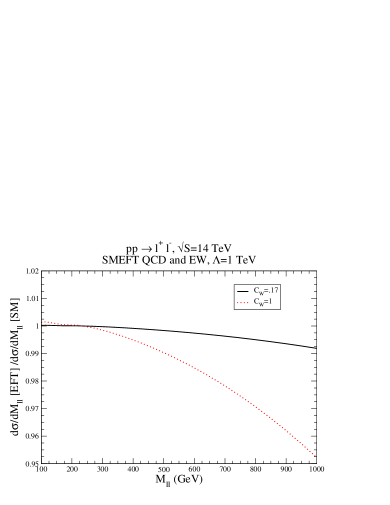
Figure 2: NLO QCD and EW SMEFT contributions to neutral DY production, normalized to the SM NLO predictions.

In Fig. 2 we show the effects of $\mathcal{C}_{\phi W}$ and ${\mathcal{C}_{\phi WB}}$ at NLO. Note that the values of $\mathcal{C}_{\phi W}$ and ${\mathcal{C}_{\phi WB}}$ that we have used are larger than those allowed by recent global fitsAlasfar:2020mne ; Ethier:2021bye , emphasizing the smallness of these effects. (An NLO fit to EWPOsDawson:2019clf gives the allowed $95\%$ CL ranges, $-.0079<\mathcal{C}_{\phi WB}<.0016$ and $-4.8<\mathcal{C}_{W}<.48$). The effects of the $C_{W}$ NLO corrections to DY are a few percent for allowed values of the coefficients. As an example, in Fig. 3 we show the size of the NLO EW effects for the case with tagged photons with $p_{T}>2~{}GeV$ for several coefficients that are poorly constrained by the global fits. The size of the effects is of the order of a few percent. It is interesting that the inclusion of the quadratic terms has a small effect. This is consistent with the results of Ethier:2021bye .

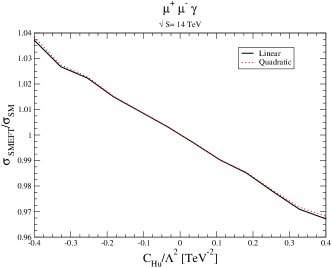
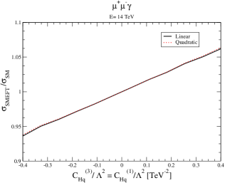
Figure 3: NLO QCD and EW SMEFT contributions to neutral DY production with a tagged $\gamma$, normalized to the SM NLO predictions, with $p_{T}>2~{}GeV$ with the linear and quadratic approximations defined as in Eqs. 5 and 6.

V Conclusions

We have calculated the complete set of NLO electroweak and QCD corrections in the SMEFT to Drell Yan production arising from bosonic operators, such as those arising in UV models with high scale vector-like fermions or scalars. The calculation of the virtual EW corrections represents a significant advance in the program of computing NLO EW effects for scattering processes in the SMEFT. Our major results are contained in the auxilliary files posted at https://quark.phy.bnl.gov/Digital_Data_Archive/dawson/drellyan_21. The results are presented in a form that can be implemented in existing Drell Yan Monte Carlo programs. Our results suggest that the NLO corrections from the bosonic operators are on the order of a few percent in DY processes and presents a target future HL-LHC DY measurements.

Appendix A Tree level SMEFT results for $q{\overline{q}}\rightarrow l^{+}l^{-}$

The tree level SMEFT results as defined in Eq. 9 for up quark initial states are,

$$\delta G_{RR}^{u} = {{\mathcal{C}_{\phi WB}}\over\Lambda^{2}}{{16\,\sqrt{w}\,\left(w-s\right)\,\sqrt{z-w}}\over{3\,s\,\left(z-s\right)}}-{\mathcal{C}_{\phi D}\over\Lambda^{2}}{4\,\left(s\,z-w^{2}\right)\over 3\,s\,\left(z-s\right)}$$

$$+{z\over 3\,\left(z-s\right)\Lambda^{2}}\biggr{(}6\,C_{\phi u,11}-4\,C_{\phi e,22}+3\,C_{eu,2211}\biggr{)}$$

$$+{1\over 3\,\left(z-s\right)\Lambda^{2}}\biggl{(}\biggl{[}-6\,C_{\phi u,11}+4\,C_{\phi e,22}\biggr{]}\,w-3\,C_{eu,2211}\,s\biggr{)}$$

$$+4\frac{(w-s)(z-w)}{3s(z-s)}\biggl{(}2(C_{\phi l,11}^{(3)}+C_{\phi l,22}^{(3)})-C_{ll,1221}-C_{ll,2112}\biggr{)}$$

$$\delta G_{LL}^{u} = {{\mathcal{C}_{\phi WB}}\over\Lambda^{2}}{{2\,\sqrt{w}\,\left(8\,w-3\,s\right)\,\sqrt{z-w}}\over{3\,s\,\left(z-s\right)}}-{{\mathcal{C}_{\phi D}}\over\Lambda^{2}}{{\left(s\,z-8\,w^{2}\right)}\over{6\,s\,\left(z-s\right)}}$$

$$-{z\over 3\,\left(z-s\right)\Lambda^{2}}\ \biggl{(}3\,C_{lq,2211}^{(3)}-3\,C_{lq,2211}^{(1)}+3\,C_{\phi q,11}^{(3)}-3C_{\phi q,11}^{(1)}+C_{\phi l,22}^{(3)}+C_{\phi l,22}^{(1)}\biggr{)}$$

$$-{w\over 3\,\left(z-s\right)\Lambda^{2}}\biggl{(}-6\,C_{\phi q,11}^{(3)}\,+6\,{C_{\phi q,11}^{(1)}\,-4\,C_{\phi l,22}^{(3)}-4\,C_{\phi l,22}^{(1)}\,\biggr{)}}$$

$$-{s\over 3\,\left(z-s\right)\Lambda^{2}}\biggl{(}-3\,C_{lq,2211}^{(3)}+3\,C_{lq,2211}^{(1)}\,\biggr{)}$$

$$-\frac{8w(w-z)+s(2w+z)}{6s(z-s)}\biggl{(}2(C_{\phi l,11}^{(3)}+C_{\phi l,22}^{(3)})-C_{ll,1221}-C_{ll,2112}\biggr{)}$$

$$\delta G_{LR}^{u} = {{\mathcal{C}_{\phi WB}}\over\Lambda^{2}}{{2\,\sqrt{w}\,\left(8\,w-5\,s\right)\,\sqrt{z-w}}\over{3\,s\,\left(z-s\right)}}-{\mathcal{C}_{\phi D}\over\Lambda^{2}}\,{\left(s\,z-4\,w^{2}\right)\over{3\,s\,\left(z-s\right)}}$$

$$+{z\over 3\,\left(z-s\right)\Lambda^{2}}\biggl{(}3\,C_{qe,1122}\,-6C_{\phi q,11}^{(3)}\,+6\,C_{\phi q,11}^{(1)}\,-C_{\phi e,22}\,\biggr{)}$$

$$+{1\over 3\,\left(z-s\right)\Lambda^{2}}\biggl{(}\biggl{[}6\,C_{\phi q,11}^{(3)}-6\,C_{\phi q,11}^{(1)}+4\,C_{\phi e,22}\biggr{]}\,w-3\,C_{qe,1122}\,s\biggr{)}$$

$$+\frac{(s-4w)(w-z)}{3s(z-s)}\biggl{(}2(C_{\phi l,11}^{(3)}+C_{\phi l,22}^{(3)})-C_{ll,1221}-C_{ll,2112}\biggr{)}$$

$$\delta G_{RL}^{u} = {{\mathcal{C}_{\phi WB}}\over\Lambda^{2}}{4\,\sqrt{w}\,\left(4\,w-3\,s\right)\,\sqrt{z-w}\over 3\,s\,\left(z-s\right)}-{\mathcal{C}_{\phi D}\over\Lambda^{2}}{2\,\,\left(s\,z-2\,w^{2}\right)\over 3\,s\,\left(z-s\right)}$$ (36)

$$+{z\over 3\,\left(z-s\right)\Lambda^{2}}\,\biggl{(}3\,C_{lu,2211}\,+3\,C_{\phi u,11}\,-4\,C_{\phi l,22}^{(3)}\,-4\,C_{\phi l,22}^{(1)}\,\biggr{)}$$

$$+{1\over 3\,\left(z-s\right)\Lambda^{2}}\biggl{(}\biggl{[}-6\,C_{\phi u,11}\,+4\,C_{\phi l,22}^{(3)}\,+4\,C_{\phi l,22}^{(1)}\,\biggr{]}w-3\,C_{lu,2211}\,s\biggr{)}$$

$$+\frac{2(s-2w)(w-z)}{3s(z-s)}\biggl{(}2(C_{\phi l,11}^{(3)}+C_{\phi l,22}^{(3)})-C_{ll,1221}-C_{ll,2112}\biggr{)}$$

and the numerical subscripts are generation indices. The results for down quark initial states are,

$$\delta G_{RR}^{d} = -{{\mathcal{C}_{\phi WB}}\over\Lambda^{2}}{{8\,\sqrt{w}\,\left(w-s\right)\,\sqrt{z-w}}\over{3\,s\,\left(z-s\right)}}+{\mathcal{C}_{\phi D}\over\Lambda^{2}}{2\,\left(s\,z-w^{2}\right)\over 3\,s\,\left(z-s\right)}$$

$$+{z\over 3\,\left(z-s\right)\Lambda^{2}}\biggr{(}6\,C_{\phi d,11}+2\,C_{\phi e,22}+3\,C_{ed,2211}\biggr{)}$$

$$+{1\over 3\,\left(z-s\right)\Lambda^{2}}\biggl{(}\biggl{[}-6\,C_{\phi d,11}-2\,C_{\phi e,22}\biggr{]}\,w-3\,C_{ed,2211}\,s\biggr{)}$$

$$-2\frac{(w-s)(z-w)}{3s(z-s)}\biggl{(}2(C_{\phi l,11}^{(3)}+C_{\phi l,22}^{(3)})-C_{ll,1221}-C_{ll,2112}\biggr{)}$$

$$\delta G_{LL}^{d} = -{{\mathcal{C}_{\phi WB}}\over\Lambda^{2}}{{2\,\sqrt{w}\,\left(4\,w\right)\,\sqrt{z-w}}\over{3\,s\,\left(z-s\right)}}-{{\mathcal{C}_{\phi D}}\over\Lambda^{2}}{{\left(s\,z+4\,w^{2}\right)}\over{6\,s\,\left(z-s\right)}}$$

$$+{z\over 3\,\left(z-s\right)\Lambda^{2}}\ \biggl{(}3\,C_{lq,2211}^{(3)}+3\,C_{lq,2211}^{(1)}+3\,C_{\phi q,11}^{(3)}+3C_{\phi q,11}^{(1)}-C_{\phi l,22}^{(3)}-C_{\phi l,22}^{(1)}\biggr{)}$$

$$-{w\over 3\,\left(z-s\right)\Lambda^{2}}\biggl{(}6\,C_{\phi q,11}^{(3)}\,+6\,{C_{\phi q,11}^{(1)}\,+2\,C_{\phi l,22}^{(3)}+2\,C_{\phi l,22}^{(1)}\,\biggr{)}}$$

$$+{s\over 3\,\left(z-s\right)\Lambda^{2}}\biggl{(}-3\,C_{lq,2211}^{(3)}-3\,C_{lq,2211}^{(1)}\,\biggr{)}$$

$$+\frac{4w(w-z)+s(4w-z)}{6s(z-s)}\biggl{(}2(C_{\phi l,11}^{(3)}+C_{\phi l,22}^{(3)})-C_{ll,1221}-C_{ll,2112}\biggr{)}$$

$$\delta G_{LR}^{d} = -{{\mathcal{C}_{\phi WB}}\over\Lambda^{2}}{{2\,\sqrt{w}\,\left(4\,w-s\right)\,\sqrt{z-w}}\over{3\,s\,\left(z-s\right)}}-{\mathcal{C}_{\phi D}\over\Lambda^{2}}\,{\left(s\,z+2\,w^{2}\right)\over{3\,s\,\left(z-s\right)}}$$

$$+{z\over 3\,\left(z-s\right)\Lambda^{2}}\biggl{(}3\,C_{qe,1122}\,+6C_{\phi q,11}^{(3)}\,+6\,C_{\phi q,11}^{(1)}\,-C_{\phi e,22}\,\biggr{)}$$

$$-{1\over 3\,\left(z-s\right)\Lambda^{2}}\biggl{(}\biggl{[}6\,C_{\phi q,11}^{(3)}+6\,C_{\phi q,11}^{(1)}+2\,C_{\phi e,22}\biggr{]}\,w+3\,C_{qe,1122}\,s\biggr{)}$$

$$+\frac{(s+2w)(w-z)}{3s(z-s)}\biggl{(}2(C_{\phi l,11}^{(3)}+C_{\phi l,22}^{(3)})-C_{ll,1221}-C_{ll,2112}\biggr{)}$$

$$\delta G_{RL}^{d} = -{{\mathcal{C}_{\phi WB}}\over\Lambda^{2}}{2\,\sqrt{w}\,\left(4\,w-3\,s\right)\,\sqrt{z-w}\over 3\,s\,\left(z-s\right)}+{\mathcal{C}_{\phi D}\over\Lambda^{2}}{\,\left(s\,z-2\,w^{2}\right)\over 3\,s\,\left(z-s\right)}$$ (37)

$$+{z\over 3\,\left(z-s\right)\Lambda^{2}}\,\biggl{(}3\,C_{ld,2211}\,+3\,C_{\phi d,11}\,+2\,C_{\phi l,22}^{(3)}\,+2\,C_{\phi l,22}^{(1)}\,\biggr{)}$$

$$+{1\over 3\,\left(z-s\right)\Lambda^{2}}\biggl{(}\biggl{[}-6\,C_{\phi d,11}\,-2\,C_{\phi l,22}^{(3)}\,-2\,C_{\phi l,22}^{(1)}\,\biggr{]}w-3\,C_{ld,2211}\,s\biggr{)}$$

$$-\frac{(s-2w)(w-z)}{3s(z-s)}\biggl{(}2(C_{\phi l,11}^{(3)}+C_{\phi l,22}^{(3)})-C_{ll,1221}-C_{ll,2112}\biggr{)}$$

.

Appendix B Real SMEFT contributions

B.1 Real Photon Emission

The SMEFT contributions to $q{\overline{q}}\rightarrow l^{+}l^{-}\gamma$ are defined in Eq. 20 and $G_{XY}^{SM}$ is defined in Eq. 12. The functions $\delta F_{XY}^{q}$ are,

$$\delta F_{XY}^{q}(s) = \frac{f^{q}_{0}}{s}+\frac{f^{q}_{XY}}{s-z}+\frac{3vG_{XY}^{SM}}{4\Lambda^{2}}\biggl{(}C_{ll,1221}+C_{ll,2112}-2(C_{\phi l,11}^{(3)}+C_{\phi l,22}^{(3)})\biggr{)}$$ (38)

(Our notation is $w=M_{W}^{2},v=(VEV)^{2}={1\over\sqrt{2}G_{\mu}},z=M_{Z}^{2}$ as in the main text.)

$$f^{u}_{0} = {2w\over z\Lambda^{2}}\biggl{(}w\mathcal{C}_{\phi D}+4(z-w){\mathcal{C}_{\phi WB}r}\biggr{)}$$

$$f^{u}_{LL} = {1\over 12z\Lambda^{2}}\biggl{\{}\mathcal{C}_{\phi D}(-24w^{3}+22w^{2}z+wz^{2}-2z^{3})/(w-z)+4\biggl{[}{\mathcal{C}_{\phi WB}r}(24w^{2}-28wz+7z^{2})$$

$$+z(z-4w)(\mathcal{C}_{\phi l22}^{(1)}+\mathcal{C}_{\phi l22}^{(3)})+3z(2w-z)(\mathcal{C}_{\phi q11}^{(1)}-\mathcal{C}_{\phi q11}^{(3)})\biggr{]}\biggr{\}}$$

$$f^{u}_{LR} = {1\over 6z\Lambda^{2}}\biggl{\{}\mathcal{C}_{\phi D}(-12w^{2}+wz+2z^{2})+24{\mathcal{C}_{\phi WB}r}(2w^{2}-3wz+z^{2})$$

$$+2z(z-4w)\mathcal{C}_{\phi e22}+12z(w-z)(\mathcal{C}_{\phi q11}^{(1)}-\mathcal{C}_{\phi q11}^{(3)})\biggr{\}}$$

$$f^{u}_{RL} = {1\over 3z\Lambda^{2}}\biggl{\{}\mathcal{C}_{\phi D}(-6w^{2}+wz+2z^{2})+8{\mathcal{C}_{\phi WB}r}(3w^{2}-5wz+2z^{2})$$

$$+(6w-3z)z\mathcal{C}_{\phi u11}+4z(z-w)(\mathcal{C}_{\phi l22}^{(1)}+\mathcal{C}_{\phi l22}^{(3)})\biggr{\}}$$

$$f^{u}_{RR} = {2(z-w)\over 3z\Lambda^{2}}\biggl{\{}(3w+2z)\mathcal{C}_{\phi D}+12(z-w){\mathcal{C}_{\phi WB}r}w+2z\mathcal{C}_{\phi e22}-3z\mathcal{C}_{\phi u11}\biggr{\}}$$ (39)

$$f^{d}_{0} =- {w\over z\Lambda^{2}}\biggl{(}w\mathcal{C}_{\phi D}+4(z-w){\mathcal{C}_{\phi WB}r}\biggr{)}$$

$$f^{d}_{LL} = {1\over 12z\Lambda^{2}}\biggl{\{}\mathcal{C}_{\phi D}(12w^{3}-8w^{2}z+wz^{2}-2z^{3})/(w-z)+4\biggl{[}{\mathcal{C}_{\phi WB}r}(-12w^{2}+8wz+z^{2})$$

$$+z(z+2w)(\mathcal{C}_{\phi l22}^{(1)}+\mathcal{C}_{\phi l22}^{(3)})+3z(2w-z)(\mathcal{C}_{\phi q11}^{(1)}+\mathcal{C}_{\phi q11}^{(3)})\biggr{]}\biggr{\}}$$

$$f^{d}_{LR} = {1\over 6z\Lambda^{2}}\biggl{\{}\mathcal{C}_{\phi D}(6w^{2}+wz+2z^{2})+24{\mathcal{C}_{\phi WB}r}w(z-w)$$

$$+2z(z+2w)\mathcal{C}_{\phi e22}+12z(w-z)(\mathcal{C}_{\phi q11}^{(1)}+\mathcal{C}_{\phi q11}^{(3)})\biggr{\}}$$

$$f^{d}_{RL} = {1\over 6z\Lambda^{2}}\biggl{\{}\mathcal{C}_{\phi D}(3w-2z)(2w+z)-8{\mathcal{C}_{\phi WB}r}(3w-2z)(w-z)$$

$$+6(2w-z)z\mathcal{C}_{\phi d11}+4z(w-z)(\mathcal{C}_{\phi l22}^{(1)}+\mathcal{C}_{\phi l22}^{(3)})\biggr{\}}$$

$$f^{d}_{RR} = {(w-z)\over 3z\Lambda^{2}}\biggl{\{}(3w+2z)\mathcal{C}_{\phi D}+12(z-w){\mathcal{C}_{\phi WB}r}w+2z\mathcal{C}_{\phi e22}+6z\mathcal{C}_{\phi d11}\biggr{\}}$$ (40)

where ${\mathcal{C}_{\phi WB}r}\equiv\sqrt{{w\over z-w}}{\mathcal{C}_{\phi WB}}$.

B.2 Real gluon emission

The total spin and color averaged amplitude squared for $q{\overline{q}}\rightarrow l^{+}l^{-}g$ is

$$\mid{\overline{A}}\mid^{2} = {C_{F}s_{34}\over 6s_{15}s_{25}}\biggl{\{}{\tilde{t}}^{2}\biggl{[}H_{LR}(s_{34})^{2}+H_{RL}(s_{34})^{2}\biggr{]}+{\tilde{u}}^{2}\biggl{[}H_{LL}(s_{34})^{2}+H_{RR}(s_{34}^{2})\biggr{]}\biggr{\}}$$ (41)

with $H_{XY}=2g_{s}(H_{XY}^{SM}+\delta H_{XY})$.

The SM contributions are

$$H_{XY}^{SM}(s_{34})=G_{XY}^{SM}(s_{34})$$ (42)

The SMEFT contributions, $\delta H_{XY}$, are,

$$\delta H^{q}_{XY}(s) = \frac{h^{q}_{0}}{s}+\frac{h^{q}_{XY}}{s-z}+\frac{vG_{XY}^{SM}}{2\Lambda^{2}}\biggl{(}C_{ll,1221}+C_{ll,2112}-2(C_{\phi l,11}^{(3)}+C_{\phi l,22}^{(3)})\biggr{)}$$ (43)

$$h^{u}_{0} = {4w\over 3z\Lambda^{2}}\biggl{\{}\mathcal{C}_{\phi D}w+4{\mathcal{C}_{\phi WB}r}(z-w)\biggr{\}}$$

$$h^{u}_{LL} = {1\over 6z\Lambda^{2}}\biggl{\{}\mathcal{C}_{\phi D}(z^{2}-8w^{2})+4{\mathcal{C}_{\phi WB}r}(8w^{2}-11wz+3z^{2})$$

$$+2z\biggl{[}(z-4w)(\mathcal{C}_{\phi l22}^{(1)}+\mathcal{C}_{\phi l22}^{(3)})+3(2w-z)(\mathcal{C}_{\phi q11}^{(1)}-\mathcal{C}_{\phi q11}^{(3)})\biggr{]}\biggr{\}}$$

$$h^{u}_{LR} = {1\over 3z\Lambda^{2}}\biggl{\{}\mathcal{C}_{\phi D}(z^{2}-4w^{2})+2{\mathcal{C}_{\phi WB}r}(8w^{2}-13wz+5z^{2})$$

$$+z\biggl{[}(z-4w)\mathcal{C}_{\phi e22}+6(w-z)(\mathcal{C}_{\phi q11}^{(1)}-\mathcal{C}_{\phi q11}^{(3)})\biggr{]}$$

$$h^{u}_{RL} = {1\over 3z\Lambda^{2}}\biggl{\{}\mathcal{C}_{\phi D}(2z^{2}-4w^{2})+4{\mathcal{C}_{\phi WB}r}(4w^{2}-7wz+3z^{2})$$

$$+z\biggl{[}4(z-w)(\mathcal{C}_{\phi l22}^{(1)}+\mathcal{C}_{\phi l22}^{(3)})+(6w-3z)\mathcal{C}_{\phi u11}\biggr{]}\biggr{\}}$$

$$h^{u}_{RR} = {2(z-w)\over 3z\Lambda^{2}}\biggl{\{}8{\mathcal{C}_{\phi WB}r}(z-w)+2\mathcal{C}_{\phi D}(w+z)+2z\mathcal{C}_{\phi e22}-3z\mathcal{C}_{\phi u11}\biggr{\}}\biggr{\}}$$ (44)

$$h^{d}_{0} = {-2w\over 3z\Lambda^{2}}\biggl{\{}\mathcal{C}_{\phi D}w+4{\mathcal{C}_{\phi WB}r}(z-w)\biggr{\}}$$

$$h^{d}_{LL} = {1\over 6z\Lambda^{2}}\biggl{\{}\mathcal{C}_{\phi D}(z^{2}+4w^{2})+16{\mathcal{C}_{\phi WB}r}w(z-w)$$

$$+2z\biggl{[}(z+2w)(\mathcal{C}_{\phi l22}^{(1)}+\mathcal{C}_{\phi l22}^{(3)})+3(2w-z)(\mathcal{C}_{\phi q11}^{(1)}+\mathcal{C}_{\phi q11}^{(3)})\biggr{]}\biggr{\}}$$

$$h^{d}_{LR} = {1\over 3z\Lambda^{2}}\biggl{\{}\mathcal{C}_{\phi D}(z^{2}+2w^{2})-2{\mathcal{C}_{\phi WB}r}(4w^{2}-5wz+z^{2})$$

$$+z\biggl{[}(z+2w)\mathcal{C}_{\phi e22}+6(w-z)(\mathcal{C}_{\phi q11}^{(1)}+\mathcal{C}_{\phi q11}^{(3)})\biggr{]}$$

$$h^{d}_{RL} = {1\over 3z\Lambda^{2}}\biggl{\{}\mathcal{C}_{\phi D}(2w^{2}-z^{2})-2{\mathcal{C}_{\phi WB}r}(4w^{2}-7wz+3z^{2})$$

$$+z\biggl{[}2(w-z)(\mathcal{C}_{\phi l22}^{(1)}+\mathcal{C}_{\phi l22}^{(3)})+(6w-3z)\mathcal{C}_{\phi d11}\biggr{]}\biggr{\}}$$

$$h^{d}_{RR} = {2(w-z)\over 3z\Lambda^{2}}\biggl{\{}4{\mathcal{C}_{\phi WB}r}(z-w)+\mathcal{C}_{\phi D}(w+z)+z\mathcal{C}_{\phi e22}+3z\mathcal{C}_{\phi d11}\biggr{\}}\biggr{\}}$$ (45)

References

- (1) G. Altarelli, R. K. Ellis, and G. Martinelli, “Large Perturbative Corrections to the Drell-Yan Process in QCD,” Nucl. Phys. B 157 (1979) 461–497.
- (2) J. Kubar-Andre and F. E. Paige, “Gluon Corrections to the Drell-Yan Model,” Phys. Rev. D 19 (1979) 221.
- (3) U. Baur, O. Brein, W. Hollik, C. Schappacher, and D. Wackeroth, “Electroweak radiative corrections to neutral current Drell-Yan processes at hadron colliders,” Phys. Rev. D 65 (2002) 033007, arXiv:hep-ph/0108274.
- (4) S. Dittmaier and M. Krämer, “Electroweak radiative corrections to W boson production at hadron colliders,” Phys. Rev. D 65 (2002) 073007, arXiv:hep-ph/0109062.
- (5) R. Hamberg, W. L. van Neerven, and T. Matsuura, “A complete calculation of the order correction to the Drell-Yan factor,” Nucl. Phys. B 359 (1991) 343–405. [Erratum: Nucl.Phys.B 644, 403–404 (2002)].
- (6) C. Anastasiou, L. J. Dixon, K. Melnikov, and F. Petriello, “Dilepton rapidity distribution in the Drell-Yan process at NNLO in QCD,” Phys. Rev. Lett. 91 (2003) 182002, arXiv:hep-ph/0306192.
- (7) C. Anastasiou, L. J. Dixon, K. Melnikov, and F. Petriello, “High precision QCD at hadron colliders: Electroweak gauge boson rapidity distributions at NNLO,” Phys. Rev. D 69 (2004) 094008, arXiv:hep-ph/0312266.
- (8) K. Melnikov and F. Petriello, “Electroweak gauge boson production at hadron colliders through ,” Physical Review D 74 no. 11, (Dec, 2006) . http://dx.doi.org/10.1103/PhysRevD.74.114017.
- (9) S. Catani, L. Cieri, G. Ferrera, D. de Florian, and M. Grazzini, “Vector boson production at hadron colliders: a fully exclusive QCD calculation at NNLO,” Phys. Rev. Lett. 103 (2009) 082001, arXiv:0903.2120 [hep-ph].
- (10) Y. Li and F. Petriello, “Combining QCD and electroweak corrections to dilepton production in FEWZ,” Phys. Rev. D 86 (2012) 094034, arXiv:1208.5967 [hep-ph].
- (11) S. Camarda et al., “DYTurbo: Fast predictions for Drell-Yan processes,” Eur. Phys. J. C 80 no. 3, (2020) 251, arXiv:1910.07049 [hep-ph]. [Erratum: Eur.Phys.J.C 80, 440 (2020)].
- (12) C. Duhr, F. Dulat, and B. Mistlberger, “Drell-Yan Cross Section to Third Order in the Strong Coupling Constant,” Phys. Rev. Lett. 125 no. 17, (2020) 172001, arXiv:2001.07717 [hep-ph].
- (13) C. Duhr, F. Dulat, and B. Mistlberger, “Charged current Drell-Yan production at N3LO,” JHEP 11 (2020) 143, arXiv:2007.13313 [hep-ph].
- (14) T. Becher and T. Neumann, “Fiducial resummation of color-singlet processes at N3LL+NNLO,” JHEP 03 (2021) 199, arXiv:2009.11437 [hep-ph].
- (15) E. Re, L. Rottoli, and P. Torrielli, “Fiducial Higgs and Drell-Yan distributions at N3LL′+NNLO with RadISH,” arXiv:2104.07509 [hep-ph].
- (16) W. Bizon, X. Chen, A. Gehrmann-De Ridder, T. Gehrmann, N. Glover, A. Huss, P. F. Monni, E. Re, L. Rottoli, and P. Torrielli, “Fiducial distributions in higgs and drell-yan production at n3ll+nnlo,” Journal of High Energy Physics 2018 no. 12, (Dec, 2018) . http://dx.doi.org/10.1007/JHEP12(2018)132.
- (17) W. B. Kilgore and C. Sturm, “Two-Loop Virtual Corrections to Drell-Yan Production at order ,” Phys. Rev. D 85 (2012) 033005, arXiv:1107.4798 [hep-ph].
- (18) F. Buccioni, F. Caola, M. Delto, M. Jaquier, K. Melnikov, and R. Röntsch, “Mixed QCD-electroweak corrections to on-shell Z production at the LHC,” Phys. Lett. B 811 (2020) 135969, arXiv:2005.10221 [hep-ph].
- (19) M. Delto, M. Jaquier, K. Melnikov, and R. Röntsch, “Mixed QCDQED corrections to on-shell boson production at the LHC,” JHEP 01 (2020) 043, arXiv:1909.08428 [hep-ph].
- (20) R. Boughezal, Y. Li, and F. Petriello, “Disentangling radiative corrections using the high-mass Drell-Yan process at the LHC,” Phys. Rev. D 89 no. 3, (2014) 034030, arXiv:1312.3972 [hep-ph].
- (21) L. Buonocore, M. Grazzini, and F. Tramontano, “The subtraction method: electroweak corrections and power suppressed contributions,” Eur. Phys. J. C 80 no. 3, (2020) 254, arXiv:1911.10166 [hep-ph].
- (22) S. Dittmaier, T. Schmidt, and J. Schwarz, “Mixed NNLO QCD×electroweak corrections of to single-W/Z production at the LHC,” JHEP 12 (2020) 201, arXiv:2009.02229 [hep-ph].
- (23) R. Bonciani, F. Buccioni, N. Rana, and A. Vicini, “Next-to-Next-to-Leading Order Mixed QCD-Electroweak Corrections to on-Shell Z Production,” Phys. Rev. Lett. 125 no. 23, (2020) 232004, arXiv:2007.06518 [hep-ph].
- (24) M. Heller, A. von Manteuffel, R. M. Schabinger, and H. Spiesberger, “Mixed EW-QCD two-loop amplitudes for and scheme independence of multi-loop corrections,” arXiv:2012.05918 [hep-ph].
- (25) A. Collaboration, “Measurement of the transverse momentum distribution of drell-yan lepton pairs in proton-proton collisions at tev with the atlas detector,” 2020.
- (26) CMS Collaboration, A. M. Sirunyan et al., “Measurement of the differential Drell-Yan cross section in proton-proton collisions at = 13 TeV,” JHEP 12 (2019) 059, arXiv:1812.10529 [hep-ex].
- (27) A. Denner and S. Pozzorini, “One-loop leading logarithms in electroweak radiative corrections,” The European Physical Journal C 18 no. 3, (Jan, 2001) 461?480. http://dx.doi.org/10.1007/s100520100551.
- (28) J. M. Campbell, D. Wackeroth, and J. Zhou, “Study of weak corrections to Drell-Yan, top-quark pair, and dijet production at high energies with MCFM,” Phys. Rev. D 94 no. 9, (2016) 093009, arXiv:1608.03356 [hep-ph].
- (29) I. Brivio and M. Trott, “The Standard Model as an Effective Field Theory,” Phys. Rept. 793 (2019) 1–98, arXiv:1706.08945 [hep-ph].
- (30) I. Brivio, “SMEFTsim 3.0 — a practical guide,” JHEP 04 (2021) 073, arXiv:2012.11343 [hep-ph].
- (31) C. Degrande, G. Durieux, F. Maltoni, K. Mimasu, E. Vryonidou, and C. Zhang, “Automated one-loop computations in the standard model effective field theory,” Phys. Rev. D 103 no. 9, (2021) 096024, arXiv:2008.11743 [hep-ph].
- (32) J. Baglio, S. Dawson, S. Homiller, S. D. Lane, and I. M. Lewis, “Validity of standard model EFT studies of VH and VV production at NLO,” Phys. Rev. D 101 no. 11, (2020) 115004, arXiv:2003.07862 [hep-ph].
- (33) J. Baglio, S. Dawson, and S. Homiller, “QCD corrections in Standard Model EFT fits to and production,” Phys. Rev. D 100 no. 11, (2019) 113010, arXiv:1909.11576 [hep-ph].
- (34) J. Baglio, S. Dawson, and I. M. Lewis, “NLO effects in EFT fits to production at the LHC,” Phys. Rev. D 99 no. 3, (2019) 035029, arXiv:1812.00214 [hep-ph].
- (35) S. Alioli, W. Dekens, M. Girard, and E. Mereghetti, “NLO QCD corrections to SM-EFT dilepton and electroweak Higgs boson production, matched to parton shower in POWHEG,” JHEP 08 (2018) 205, arXiv:1804.07407 [hep-ph].
- (36) J. M. Cullen and B. D. Pecjak, “Higgs decay to fermion pairs at NLO in SMEFT,” JHEP 11 (2020) 079, arXiv:2007.15238 [hep-ph].
- (37) J. M. Cullen, B. D. Pecjak, and D. J. Scott, “NLO corrections to decay in SMEFT,” JHEP 08 (2019) 173, arXiv:1904.06358 [hep-ph].
- (38) R. Gauld, B. D. Pecjak, and D. J. Scott, “QCD radiative corrections for in the Standard Model Dimension-6 EFT,” Phys. Rev. D 94 no. 7, (2016) 074045, arXiv:1607.06354 [hep-ph].
- (39) C. Hartmann and M. Trott, “Higgs decay to two photons at one loop in the standard model effective field theory,” Physical Review Letters 115 no. 19, (Nov, 2015) . http://dx.doi.org/10.1103/PhysRevLett.115.191801.
- (40) C. Hartmann and M. Trott, “On one-loop corrections in the standard model effective field theory; the ?(h ? ??) case,” Journal of High Energy Physics 2015 no. 7, (Jul, 2015) . http://dx.doi.org/10.1007/JHEP07(2015)151.
- (41) S. Dawson and P. P. Giardino, “Electroweak corrections to Higgs boson decays to and in standard model EFT,” Phys. Rev. D 98 no. 9, (2018) 095005, arXiv:1807.11504 [hep-ph].
- (42) A. Dedes, M. Paraskevas, J. Rosiek, K. Suxho, and L. Trifyllis, “The decay in the Standard-Model Effective Field Theory,” JHEP 08 (2018) 103, arXiv:1805.00302 [hep-ph].
- (43) S. Dawson and P. P. Giardino, “Higgs decays to and in the standard model effective field theory: An NLO analysis,” Phys. Rev. D 97 no. 9, (2018) 093003, arXiv:1801.01136 [hep-ph].
- (44) A. Dedes, K. Suxho, and L. Trifyllis, “The decay in the Standard-Model Effective Field Theory,” JHEP 06 (2019) 115, arXiv:1903.12046 [hep-ph].
- (45) S. Dawson and P. P. Giardino, “Electroweak and QCD corrections to and pole observables in the standard model EFT,” Phys. Rev. D 101 no. 1, (2020) 013001, arXiv:1909.02000 [hep-ph].
- (46) C. Hartmann, W. Shepherd, and M. Trott, “The decay width in the SMEFT: and corrections at one loop,” JHEP 03 (2017) 060, arXiv:1611.09879 [hep-ph].
- (47) R. Boughezal, C.-Y. Chen, F. Petriello, and D. Wiegand, “Top quark decay at next-to-leading order in the Standard Model Effective Field Theory,” Phys. Rev. D 100 no. 5, (2019) 056023, arXiv:1907.00997 [hep-ph].
- (48) S. Dawson, P. P. Giardino, and A. Ismail, “Standard model EFT and the Drell-Yan process at high energy,” Phys. Rev. D 99 no. 3, (2019) 035044, arXiv:1811.12260 [hep-ph].
- (49) G. Panico, L. Ricci, and A. Wulzer, “High-energy EFT probes with fully differential Drell-Yan measurements,” JHEP 07 (2021) 086, arXiv:2103.10532 [hep-ph].
- (50) R. Torre, L. Ricci, and A. Wulzer, “On the W&Y interpretation of high-energy Drell-Yan measurements,” JHEP 02 (2021) 144, arXiv:2008.12978 [hep-ph].
- (51) J. de Blas, M. Chala, and J. Santiago, “Global Constraints on Lepton-Quark Contact Interactions,” Phys. Rev. D 88 (2013) 095011, arXiv:1307.5068 [hep-ph].
- (52) J. D. Wells and Z. Zhang, “Effective theories of universal theories,” JHEP 01 (2016) 123, arXiv:1510.08462 [hep-ph].
- (53) J. de Blas, J. C. Criado, M. Perez-Victoria, and J. Santiago, “Effective description of general extensions of the Standard Model: the complete tree-level dictionary,” JHEP 03 (2018) 109, arXiv:1711.10391 [hep-ph].
- (54) W. Buchmuller and D. Wyler, “Effective Lagrangian Analysis of New Interactions and Flavor Conservation,” Nucl. Phys. B268 (1986) 621–653.
- (55) B. Grzadkowski, M. Iskrzynski, M. Misiak, and J. Rosiek, “Dimension-Six Terms in the Standard Model Lagrangian,” JHEP 10 (2010) 085, arXiv:1008.4884 [hep-ph].
- (56) A. Dedes, W. Materkowska, M. Paraskevas, J. Rosiek, and K. Suxho, “Feynman rules for the Standard Model Effective Field Theory in Rξ -gauges,” JHEP 06 (2017) 143, arXiv:1704.03888 [hep-ph].
- (57) R. Alonso, E. E. Jenkins, A. V. Manohar, and M. Trott, “Renormalization Group Evolution of the Standard Model Dimension Six Operators III: Gauge Coupling Dependence and Phenomenology,” JHEP 04 (2014) 159, arXiv:1312.2014 [hep-ph].
- (58) I. Brivio and M. Trott, “Scheming in the SMEFT… and a reparameterization invariance!,” JHEP 07 (2017) 148, arXiv:1701.06424 [hep-ph]. [Addendum: JHEP 05, 136 (2018)].
- (59) G. Degrassi, P. Gambino, and P. P. Giardino, “The interdependence in the Standard Model: a new scrutiny,” JHEP 05 (2015) 154, arXiv:1411.7040 [hep-ph].
- (60) R. Boughezal, E. Mereghetti, and F. Petriello, “Dilepton production in the SMEFT at ,” arXiv:2106.05337 [hep-ph].
- (61) L. Berthier and M. Trott, “Consistent constraints on the Standard Model Effective Field Theory,” JHEP 02 (2016) 069, arXiv:1508.05060 [hep-ph].
- (62) M. Carpentier and S. Davidson, “Constraints on two-lepton, two quark operators,” Eur. Phys. J. C 70 (2010) 1071–1090, arXiv:1008.0280 [hep-ph].
- (63) A. Falkowski, M. González-Alonso, and K. Mimouni, “Compilation of low-energy constraints on 4-fermion operators in the SMEFT,” JHEP 08 (2017) 123, arXiv:1706.03783 [hep-ph].
- (64) V. Cirigliano, M. Gonzalez-Alonso, and M. L. Graesser, “Non-standard Charged Current Interactions: beta decays versus the LHC,” JHEP 02 (2013) 046, arXiv:1210.4553 [hep-ph].
- (65) S. Dawson and C. W. Murphy, “Standard Model EFT and Extended Scalar Sectors,” Phys. Rev. D 96 no. 1, (2017) 015041, arXiv:1704.07851 [hep-ph].
- (66) J. de Blas, M. Chala, M. Perez-Victoria, and J. Santiago, “Observable Effects of General New Scalar Particles,” JHEP 04 (2015) 078, arXiv:1412.8480 [hep-ph].
- (67) S. Alioli, M. Farina, D. Pappadopulo, and J. T. Ruderman, “Catching a New Force by the Tail,” Phys. Rev. Lett. 120 no. 10, (2018) 101801, arXiv:1712.02347 [hep-ph].
- (68) V. Bresó-Pla, A. Falkowski, and M. González-Alonso, “ in the SMEFT: precision Z physics at the LHC,” arXiv:2103.12074 [hep-ph].
- (69) S. Dawson and A. Ismail, “Standard model EFT corrections to Z boson decays,” Phys. Rev. D 98 no. 9, (2018) 093003, arXiv:1808.05948 [hep-ph].
- (70) M. Farina, G. Panico, D. Pappadopulo, J. T. Ruderman, R. Torre, and A. Wulzer, “Energy helps accuracy: electroweak precision tests at hadron colliders,” Phys. Lett. B 772 (2017) 210–215, arXiv:1609.08157 [hep-ph].
- (71) U. Baur, S. Keller, and D. Wackeroth, “Electroweak radiative corrections to boson production in hadronic collisions,” Phys. Rev. D 59 (1999) 013002, arXiv:hep-ph/9807417.
- (72) S. Dittmaier and M. Huber, “Radiative corrections to the neutral-current Drell-Yan process in the Standard Model and its minimal supersymmetric extension,” JHEP 01 (2010) 060, arXiv:0911.2329 [hep-ph].
- (73) G. ’t Hooft and M. J. G. Veltman, “Regularization and Renormalization of Gauge Fields,” Nucl. Phys. B 44 (1972) 189–213.
- (74) P. Breitenlohner and D. Maison, “Dimensional Renormalization and the Action Principle,” Commun. Math. Phys. 52 (1977) 11–38.
- (75) S. A. Larin, “The Renormalization of the axial anomaly in dimensional regularization,” Phys. Lett. B 303 (1993) 113–118, arXiv:hep-ph/9302240.
- (76) C.-Y. Chen, S. Dawson, and C. Zhang, “Electroweak Effective Operators and Higgs Physics,” Phys. Rev. D 89 no. 1, (2014) 015016, arXiv:1311.3107 [hep-ph].
- (77) M. Ghezzi, R. Gomez-Ambrosio, G. Passarino, and S. Uccirati, “NLO Higgs effective field theory and -framework,” JHEP 07 (2015) 175, arXiv:1505.03706 [hep-ph].
- (78) E. E. Jenkins, A. V. Manohar, and M. Trott, “Renormalization Group Evolution of the Standard Model Dimension Six Operators I: Formalism and lambda Dependence,” JHEP 10 (2013) 087, arXiv:1308.2627 [hep-ph].
- (79) E. E. Jenkins, A. V. Manohar, and M. Trott, “Renormalization Group Evolution of the Standard Model Dimension Six Operators II: Yukawa Dependence,” JHEP 01 (2014) 035, arXiv:1310.4838 [hep-ph].
- (80) A. Alloul, N. D. Christensen, C. Degrande, C. Duhr, and B. Fuks, “FeynRules 2.0 - A complete toolbox for tree-level phenomenology,” Comput. Phys. Commun. 185 (2014) 2250–2300, arXiv:1310.1921 [hep-ph].
- (81) T. Hahn, “Generating Feynman diagrams and amplitudes with FeynArts 3,” Comput. Phys. Commun. 140 (2001) 418–431, arXiv:hep-ph/0012260.
- (82) G. Passarino and M. J. G. Veltman, “One Loop Corrections for e+ e- Annihilation Into mu+ mu- in the Weinberg Model,” Nucl. Phys. B 160 (1979) 151–207.
- (83) V. Shtabovenko, R. Mertig, and F. Orellana, “FeynCalc 9.3: New features and improvements,” Comput. Phys. Commun. 256 (2020) 107478, arXiv:2001.04407 [hep-ph].
- (84) A. Denner and S. Dittmaier, “Electroweak Radiative Corrections for Collider Physics,” Phys. Rept. 864 (2020) 1–163, arXiv:1912.06823 [hep-ph].
- (85) A. Denner, “Techniques for the calculation of electroweak radiative corrections at the one-loop level and results for w-physics at lep200,” 2007.
- (86) B. W. Harris and J. F. Owens, “The Two cutoff phase space slicing method,” Phys. Rev. D 65 (2002) 094032, arXiv:hep-ph/0102128.
- (87) S. Carrazza, R. K. Ellis, and G. Zanderighi, “QCDLoop: a comprehensive framework for one-loop scalar integrals,” Comput. Phys. Commun. 209 (2016) 134–143, arXiv:1605.03181 [hep-ph].
- (88) L. Alasfar, A. Azatov, J. de Blas, A. Paul, and M. Valli, “ anomalies under the lens of electroweak precision,” JHEP 12 (2020) 016, arXiv:2007.04400 [hep-ph].
- (89) J. J. Ethier, G. Magni, F. Maltoni, L. Mantani, E. R. Nocera, J. Rojo, E. Slade, E. Vryonidou, and C. Zhang, “Combined SMEFT interpretation of Higgs, diboson, and top quark data from the LHC,” arXiv:2105.00006 [hep-ph].