Pointwise-in-time a posteriori error control
for time-fractional parabolic equations

Abstract

For time-fractional parabolic equations with a Caputo time derivative of order $\alpha\in(0,1)$, we give pointwise-in-time a posteriori error bounds in the spatial $L_{2}$ and $L_{\infty}$ norms. Hence, an adaptive mesh construction algorithm is applied for the L1 method, which yields optimal convergence rates $2-\alpha$ in the presence of solution singularities.

1 Introduction

Consider a fractional-order parabolic equation, of order $\alpha\in(0,1)$, of the form

$$D_{t}^{\alpha}u+{\mathcal{L}}u=f(x,t)\qquad\mbox{for}\;\;(x,t)\in\Omega\times(0,T],$$ (1.1)

subject to the initial condition $u(\cdot,0)=u_{0}$ in $\Omega$, and the boundary condition $u=0$ on $\partial\Omega$ for $t>0$. This problem is posed in a bounded Lipschitz domain $\Omega\subset\mathbb{R}^{d}$ (where $d\in\{1,2,3\}$), and involves a spatial linear second-order elliptic operator ${\mathcal{L}}$. The Caputo fractional derivative in time, denoted here by $D_{t}^{\alpha}$, is defined [2], for $t>0$, by

$$D_{t}^{\alpha}u:=J_{t}^{1-\alpha}(\partial_{t}u),\qquad J_{t}^{1-\alpha}v(\cdot,t):=\frac{1}{\Gamma(1-\alpha)}\int_{0}^{t}(t-s)^{-\alpha}\,v(\cdot,s)\,ds,$$ (1.2)

where $\Gamma(\cdot)$ is the Gamma function, and $\partial_{t}$ denotes the partial derivative in $t$.

Although there is a substantial literature on the a posteriori error estimation for classical parabolic equations, the pointwise-in-time a posteriori error control appears an open question for equations of type (1.1) (the few papers for similar problems give error estimates in global fractional Sobolev space norms [13]).

In this paper, we shall address this question by deriving pointwise-in-time a posteriori error bounds in the $L_{2}(\Omega)$ and $L_{\infty}(\Omega)$ norms. Furthermore, explicit upper barriers on the residual will be obtained that guarantee that the error remains within a prescribed tolerance and within certain desirable pointwise-in-time error profiles. These residual barriers naturally lead to an adaptive mesh construction algorithm, which will be applied for the popular L1 method. It will be demonstrated that the constructed adaptive meshes successfully detect solution singularities and yield optimal convergence rates $2-\alpha$, with the error profiles in remarkable agreement with the target.

The advantages of the proposed approach include: + no need to store past values of the sampled residual (even though the latter affects the local increments in the error non-locally); + applicability to wide classes of time discretizations; + low regularity assumptions; + the approach works seamlessly for arbitrarily large times.

Notation. We use the standard inner product $\langle\cdot,\cdot\rangle$ and the norm $\|\cdot\|$ in the space $L_{2}(\Omega)$, as well as the standard spaces $L_{\infty}(\Omega)$, $H^{1}_{0}(\Omega)$, $L_{\infty}(0,t;\,L_{2}(\Omega))$, and $W^{1,\infty}(t^{\prime},t^{\prime\prime};\,L_{2}(\Omega))$. The notation $v^{+}:=\max\{0,\,v\}$ is used for the positive part of a generic function $v$.

2 A posteriori error estimates in the $L_{2}(\Omega)$ norm

Given a solution approximation $u_{h}$ such that $u_{h}=u$ for $t=0$ and on $\partial\Omega$, we shall use its residual $R_{h}(\cdot,t):=(D_{t}^{\alpha}+{\mathcal{L}})u_{h}(\cdot,t)-f(\cdot,t)$ for $t>0$, as well as the operator

$$(D_{t}^{\alpha}+\lambda)^{-1}v(t):=\int_{0}^{t}\!(t-s)^{\alpha-1}\,E_{\alpha,\alpha}(-\lambda[t-s]^{\alpha})\,v(s)\,ds\quad\;\;\mbox{for}\;t>0.$$ (2.1)

Here $E_{\alpha,\beta}(s)=\sum_{k=0}^{\infty}\{\Gamma(\alpha k+\beta)\}^{-1}s^{k}$ is a generalized Mittag-Leffler function. A comparison with (1.2) shows that $(D_{t}^{\alpha}+0)^{-1}:=J_{t}^{\alpha}$.

Remark 2.1.

Note [2, Remark 7.1], [10, (2.11)] that (2.1) gives a solution of the equation $(D_{t}^{\alpha}+\lambda)w(t)=v(t)$ for $t>0$ subject to $w(0)=0$. Also, $E_{\alpha,\alpha}$ in (2.1) is positive $\forall\,\lambda\in\mathbb{R}$ [10, Lemma 3.3]; hence, $v\geq 0$ implies $w\geq 0$.

The main results of the paper are as follows.

Theorem 2.2.

Let ${\mathcal{L}}$ in (1.1), for some $\lambda\in\mathbb{R}$, satisfy $\langle{\mathcal{L}}v,v\rangle\geq\lambda\|v\|^{2}$ $\forall\,v\in H_{0}^{1}(\Omega)$. Suppose a unique solution $u$ of (1.1) and its approximation $u_{h}$ are in $L_{\infty}(0,t;\,L_{2}(\Omega))\cap W^{1,\infty}(\epsilon,t;\,L_{2}(\Omega))$ for any $0<\epsilon<t\leq T$, and also in $H^{1}_{0}(\Omega)$ for any $t>0$, while $u_{h}(\cdot,0)=u_{0}$ and $R_{h}(\cdot,t)=(D_{t}^{\alpha}+{\mathcal{L}})u_{h}(\cdot,t)-f(\cdot,t)$. Then

$$\|(u_{h}-u)(\cdot,t)\|\leq(D_{t}^{\alpha}+\lambda)^{-1}\|R_{h}(\cdot,t)\|\qquad\mbox{for}\;\;t>0.$$ (2.2)

Corollary 2.3.

Under the conditions of Theorem 2.2, if $\|R_{h}(\cdot,t)\|\leq(D_{t}^{\alpha}+\lambda){\mathcal{E}}(t)$ $\forall\,t>0$ for some barrier function ${\mathcal{E}}(t)\geq 0$ $\forall\,t\geq 0$, then $\|(u_{h}-u)(\cdot,t)\|\leq{\mathcal{E}}(t)$ $\forall\,t\geq 0$.

The above corollary may seem to imply that one can get any desirable pointwise-in-time error profile ${\mathcal{E}}(t)$ on demand. The tricky part is to ensure that $(D_{t}^{\alpha}+\lambda){\mathcal{E}}(t)>0$ for $t>0$, which is not true for a general positive ${\mathcal{E}}$. Two possible error profiles will be described by the following result.

Corollary 2.4.

Under the conditions of Theorem 2.2 with $\lambda\geq 0$, for the error $e=u_{h}-u$ one has

$$\|e(\cdot,t)\|\leq\sup_{0<s\leq t}\!\left\{\frac{\|R_{h}(\cdot,s)\|}{{\mathcal{R}}_{0}(s)}\right\}, \|e(\cdot,t)\|\leq t^{\alpha-1}\!\sup_{0<s\leq t}\!\left\{\frac{\|R_{h}(\cdot,s)\|}{{\mathcal{R}}_{1}(s)}\right\},$$ (2.3a)

$${\mathcal{R}}_{0}(t):=\{\Gamma(1-\alpha)\}^{-1}\,t^{-\alpha}+\lambda, {\mathcal{R}}_{1}(t):=\{\Gamma(1-\alpha)\}^{-1}\,t^{-1}\rho(\tau/t)+\lambda\,{\mathcal{E}}_{1}(t),$$ (2.3b)

$${\mathcal{E}}_{1}(t):=\max\{\tau,t\}^{\alpha-1},\quad\rho(s):=s^{-\beta}[1-((1-s)^{+})^{\beta}]\geq s^{-\beta}\min\{\beta s,\,1\},\quad\beta:=1-\alpha,$$ (2.3c)

where $$\tau>0 t^{\alpha-1} {\mathcal{E}}_{1}(t)$$ is an arbitrary parameter (and in (2.3a) can be replaced by ).

Corollary 2.5 ($u_{h}(\cdot,0)\neq u_{0}$).

Suppose that $u_{h}$ is continuous in $t$ for $t\geq 0$ and does not satisfy $u_{h}(\cdot,0)=u_{0}$. Then Theorem 2.2 and Corollaries 2.3 and 2.4 are valid with $R_{h}(\cdot,t)=[u_{h}(\cdot,0)-u_{0}]\{\Gamma(1-\alpha)\}^{-1}t^{-\alpha}+(D_{t}^{\alpha}+{\mathcal{L}})u_{h}(\cdot,t)-f(\cdot,t)$.

Remark 2.6 (${\mathcal{R}}_{0}$ v ${\mathcal{R}}_{1}$).

If uniform-in-time accuracy is targeted, then the first bound in (2.3a), with the residual barrier ${\mathcal{R}}_{0}$, is to be employed. The second bound, with ${\mathcal{R}}_{1}$, is less intuitive. It may be viewed as an a posteriori analogue of pointwise-in-time a priori error bounds of type [8, (3.2)] and [6, (4.2)] on graded meshes $\{T(j/M)^{r}\}_{j=0}^{M}$. Let $q$ denote the order of the method (with $q=2$ for the L1 method). The latter bounds show (for three discretizations) that the error behaves as $t^{{\alpha-1}}M^{-r}$ for $1\leq r\leq q-\alpha$ (with a logarithmic factor for $r=q-\alpha$), while the optimal convergence rate $q-\alpha$ in positive time is attained if $r\approx q-\alpha$. Hence, it is reasonable to expect that an adaptive algorithm using residual barriers ${\mathcal{R}}_{0}$ and ${\mathcal{R}}_{1}$ will respectively yield optimal convergence rates $q-\alpha$ globally or in positive time. This agrees, and remarkably well, with the numerical results in §4 for the L1 method, and in [3] for a number of higher-order methods.

Remark 2.7 (${\mathcal{L}}u_{0}\not\in L_{2}(\Omega)$).

If $u_{0}$ is not sufficiently smooth (see, e.g., test problem C in §4.2), then (depending on the interpolation of $u_{h}$ in time) the residual $R_{h}(\cdot,t)$ on the first time interval $(0,t_{1})$ may fail to be in $L_{2}(\Omega)$. One way to rectify this is to reset $u_{h}(\cdot,t):=u_{h}(\cdot,t_{1})$ for $t\in(0,t_{1}]$. With this modification, all above results become applicable. Importantly, all changes in $u_{h}$ need to be reflected when computing its residual $R_{h}$; in particular, as $u_{h}$ has been made discontinuous at $t=0$, Corollary 2.5 is to be employed.

The remainder of this section is devoted to the proofs of the above results. The key role will be played by the following auxiliary lemma, a discrete version of which has been useful in the a priori error analysis; see, e.g., in [5, (3.4)].

Lemma 2.8.

Suppose that $v(\cdot,0)=0$ and $v\in L_{\infty}(0,t;\,L_{2}(\Omega))\cap W^{1,\infty}(\epsilon,t;\,L_{2}(\Omega))$ for any $0<\epsilon<t\leq T$. Then

$$\langle D_{t}^{\alpha}v(\cdot,t),\,v(\cdot,t)\rangle\geq\bigl{(}D_{t}^{\alpha}\|v(\cdot,t)\|\bigr{)}\|v(\cdot,t)\|\qquad\mbox{for}\;\;t>0.$$

Proof.

In view of (1.2), replacing $\partial_{s}v(\cdot,s)$ in $D_{t}^{\alpha}v(\cdot,t)$ by $\partial_{s}\{v(\cdot,s)-v(\cdot,t)\}$ and then integrating by parts (with $v(\cdot,0)=0$), one gets

$$\Gamma(1-\alpha)\,D_{t}^{\alpha}v(\cdot,t)=t^{-\alpha}v(\cdot,t)+\int_{0}^{t}\!\alpha(t-s)^{-\alpha-1}\,\{v(\cdot,t)-v(\cdot,s)\}\,ds.$$ (2.4)

It remains to take the inner product of (2.4) with $v(\cdot,t)$. Then in the right-hand side $v(\cdot\,t)$ becomes $\|v(\cdot,t)\|^{2}$, while $\langle v(\cdot,t)-v(\cdot,s),\,v(\cdot,t)\rangle\geq\{\|v(\cdot,t)\|-\|v(\cdot\,s)\|\}\|v(\cdot,t)\|$, so the desired assertion follows. Note that the inner product of (2.4) with $v(\cdot,t)$ is well-defined, in view of $\|v(t)-v(s)\|\leq C_{t}(t-s)$ for any fixed $t>0$ (with a $t$-dependent constant $C_{t}$). Similarly, a version of (2.4) for $D_{t}^{\alpha}\|v(\cdot,t)\|$ remains well-defined as $|\,\|v(\cdot,t)\|-\|v(\cdot,s)\|\,|\leq\|v(\cdot,t)-v(\cdot,s)\|$. ∎

Remark 2.9.

One may consider (2.4) an alternative definition of $D_{t}^{\alpha}$ (with an obvious modification for the case $v(\cdot,0)\neq 0$; see also [1]), which can be applied to less smooth functions, including functions discontinuous at $t=0$. Consider ${\mathcal{E}}_{0}(t):=1$ for $t>0$ with ${\mathcal{E}}_{0}(0):=0$. Then, a calculation using (2.4) yields $\Gamma(1-\alpha)\,D_{t}^{\alpha}{\mathcal{E}}_{0}(t)=t^{-\alpha}$. The same result may be obtained using the original definition (1.2) combined with $\partial_{t}{\mathcal{E}}_{0}(t)=\delta(t)$, the Dirac delta-function, or representing ${\mathcal{E}}_{0}$ as the limit of a sequence of continuous piecewise-linear functions (similarly to [7, Remark 2.4]).

Proof of Theorem 2.2.  Set $e:=u_{h}-u$. Then $e(\cdot,0)=0$ and $(D_{t}^{\alpha}+{\mathcal{L}})e(\cdot,t)=R_{h}(\cdot,t)$ for $t>0$ subject to $e=0$ on $\partial\Omega$. Taking the inner product of this equation with $e(\cdot,t)$, then applying Lemma 2.8 and $\langle{\mathcal{L}}e,e\rangle\geq\lambda\|e\|^{2}$, one arrives at

$$(D_{t}^{\alpha}+\lambda)\|e(\cdot,t)\|\leq\|R_{h}(\cdot,t)\|\qquad\mbox{for}\;\;t>0.$$ (2.5)

Now, in view of Remark 2.1, $(D_{t}^{\alpha}+\lambda)\bigl{\{}(D_{t}^{\alpha}+\lambda)^{-1}\|R_{h}(\cdot,t)\|-\|e(\cdot,t)\|\bigr{\}}\geq 0$ yields the desired bound (2.2). $\square$

Proof of Corollary 2.3.  First, suppose that ${\mathcal{E}}(0)=0$. Then, by (2.5) combined with the corollary hypothesis, $(D_{t}^{\alpha}+\lambda)({\mathcal{E}}(t)-\|e(\cdot,t)\|)\geq 0$ subject to ${\mathcal{E}}(0)-\|e(\cdot,0)\|=0$. In view of Remark 2.1, this immediately yields the desired assertion ${\mathcal{E}}(t)-\|e(\cdot,t)\|\geq 0$. Otherwise, if ${\mathcal{E}}(0)>0$, then ${\mathcal{E}}(t)-\|e(\cdot,t)\|$ will include an additional positive component ${\mathcal{E}}(0)\,E_{\alpha,1}(-\lambda t^{\alpha})$, so ${\mathcal{E}}(t)-\|e(\cdot,t)\|$ will remain positive. $\square$

Proof of Corollary 2.4.  As all operators are linear, it suffices to prove (2.3) with the $\sup\{\cdot\}$ terms equal to $1$, i.e. for $\|R_{h}(\cdot,t)\|\leq{\mathcal{R}}_{p}(t)$, $p=0,1$.

For the first bound in (2.3a), recall from Remark 2.9 that for the function ${\mathcal{E}}_{0}(t):=1$ for $t>0$ with ${\mathcal{E}}_{0}(0):=0$ one has $(D_{t}^{\alpha}+\lambda){\mathcal{E}}_{0}(t)={\mathcal{R}}_{0}(t)$. So an application of Corollary 2.3 with ${\mathcal{E}}(t):={\mathcal{E}}_{0}(t)$ yields the first desired bound $\|e(\cdot,t)\|\leq{\mathcal{E}}_{0}(t)=1$ for $t>0$.

For the second bound in (2.3a), set ${\mathcal{E}}_{1}(t):=\max\{\tau,t\}^{\alpha-1}$ for $t>0$ with ${\mathcal{E}}_{1}(0):=0$ (a similar barrier was used in [5, Appendix A], [8, Lemma 2.3]). Now it suffices to check that $D_{t}^{\alpha}{\mathcal{E}}_{1}(t)=\{\Gamma(1-\alpha)\}^{-1}\,t^{-1}\rho(\tau/t)$, as then $(D_{t}^{\alpha}+\lambda){\mathcal{E}}_{1}(t)={\mathcal{R}}_{1}(t)\geq\|R_{h}\|$, so an application of Corollary 2.3 immediately yields the desired bound $\|e(\cdot,t)\|\leq{\mathcal{E}}_{1}(t)\leq t^{\alpha-1}$.

To evaluate $D_{t}^{\alpha}{\mathcal{E}}_{1}(t)$, set $\hat{\tau}:=\tau/t$, and note that ${\mathcal{E}}_{1}(t)=\tau^{-\beta}{\mathcal{E}}_{0}(t)-(\tau^{-\beta}-t^{-\beta})^{+}$. Then for $t\leq\tau$, i.e. $\hat{\tau}\geq 1$, one has ${\mathcal{E}}_{1}(t):=\tau^{-\beta}{\mathcal{E}}_{0}(t)$, so $\Gamma(1-\alpha)D_{t}^{\alpha}{\mathcal{E}}_{1}(t)=\tau^{-\beta}t^{-\alpha}=t^{-1}\hat{\tau}^{-\beta}=t^{-1}\rho(\hat{\tau})$ as required. For $t>\tau$, i.e. $\hat{\tau}\in(0,1)$, note that $\partial_{s}(\tau^{-\beta}-s^{-\beta})^{+}=-\partial_{s}(s^{-\beta})=\beta s^{-\beta-1}$, so

$$\Gamma(1-\alpha)\,D^{\alpha}_{t}{\mathcal{E}}_{1}(t)=t^{-1}\hat{\tau}^{-\beta}-\beta\int_{\tau}^{t}\!s^{-\beta-1}(t-s)^{-\alpha}\,ds=t^{-1}\hat{\tau}^{-\beta}\bigl{[}1-(1-\hat{\tau})^{\beta}\bigr{]},\vspace{-0.15cm}$$

so we again get $\Gamma(1-\alpha)\,D^{\alpha}_{t}{\mathcal{E}}_{1}(t)=t^{-1}\rho(\hat{\tau})$. So indeed, $D_{t}^{\alpha}{\mathcal{E}}_{1}(t)=\{\Gamma(1-\alpha)\}^{-1}\,t^{-1}\rho(\tau/t)$ for any $t>0$, as required. $\square$

Proof of Corollary 2.5.  Theorem 2.2 and its two corollaries immediately apply to $u_{h}$ once it is reset to $u_{0}$ at $t=0$ (after which, it is worth noting, $u_{h}$ becomes right-discontinuous at $t=0$). However, this modification of $u_{h}$ needs to be reflected in the computation of the residual $R_{h}$ as follows. Given $u_{h}$, continuous in $t$ for $t\geq 0$, set $\bar{u}_{h}:=u_{h}$, and then reset $u_{h}(\cdot,0):=u_{0}$ (so $\bar{u}_{h}$ is continuous for $t\geq 0$, while $u_{h}$ is continuous and equal to $\bar{u}_{h}$ for $t>0$). Now, the residual $R_{h}$ of $u_{h}$ for $t>0$ is computed using $u_{h}=[u_{h}(\cdot,0^{+})-u_{0}]({\mathcal{E}}_{0}-1)+\bar{u}_{h}$, so $D_{t}^{\alpha}u_{h}=[u_{h}(\cdot,0^{+})-u_{0}]D_{t}^{\alpha}{\mathcal{E}}_{0}+D_{t}^{\alpha}\bar{u}_{h}$, where $D_{t}^{\alpha}{\mathcal{E}}_{0}=\{\Gamma(1-\alpha)\}^{-1}t^{-\alpha}$; see Remark 2.9. In other words, to compensate for $u_{h}(\cdot,0^{+})\neq u_{0}$, one needs to add $[u_{h}(\cdot,0^{+})-u_{0}]\{\Gamma(1-\alpha)\}^{-1}t^{-\alpha}$ to $R_{h}$ of Theorem 2.2. $\square$

3 Generalization for the $L_{\infty}(\Omega)$ norm

Let ${\mathcal{L}}u:=\sum_{k=1}^{d}\Bigl{\{}-a_{k}(x)\,\partial^{2}_{x_{k}}\!u+b_{k}(x)\,\partial_{x_{k}}\!u\Bigr{\}}+c(x)\,u$ in (1.1), with sufficiently smooth coefficients $\{a_{k}\}$, $\{b_{k}\}$ and $c$ in $C(\bar{\Omega})$, for which we assume that $a_{k}>0$ in $\bar{\Omega}$, and also $c\geq\lambda\geq 0$ (while $\langle{\mathcal{L}}v,v\rangle\geq\lambda\|v\|^{2}$ is not required in this section).

Lemma 3.1 (maximum/comparison principle).

Suppose that $v(x,t)\geq 0$ for $t=0$ and $x\in\partial\Omega$, and $v$ is in $C(\bar{\Omega}\times[0,t])\cap W^{1,\infty}(\epsilon,t;\,L_{\infty}(\Omega))$ for any $0<\epsilon<t\leq T$ and also in $C^{2}(\Omega)$ for any $t>0$. Then $(D_{t}^{\alpha}+{\mathcal{L}})v\geq 0$ in $(0,T]\times\Omega$ implies $v\geq 0$ in $[0,T]\times\bar{\Omega}$.

Proof.

This result is given in [9, Theorem 2] under a stronger condition that $v(x,\cdot)\in C^{1}(0,T]\cap W^{1,1}(0,T)$. An inspection of the proof shows that this condition is only required to apply [9, Theorem 1] (the maximum principle for $D_{t}^{\alpha}$). The proof of the latter relies on the representation of type (2.4) and remains valid under our weaker assumptions. (A similar, but not identical, result is also given in [1, Theorem 4.1].) ∎

Theorem 3.2.

Under the above assumptions on ${\mathcal{L}}$, let a unique solution $u$ of (1.1) and its approximation $u_{h}$ be in $C(\bar{\Omega}\times[0,t])\cap W^{1,\infty}(\epsilon,t;\,L_{\infty}(\Omega))$ for any $0<\epsilon<t\leq T$, and also in $C^{2}(\Omega)$ for any $t>0$. Then the error bounds of Theorem 2.2 and Corollaries 2.3 and 2.4 remain true with $\|\cdot\|=\|\cdot\|_{L_{2}(\Omega)}$ replaced by $\|\cdot\|_{L_{\infty}(\Omega)}$.

Proof.

We shall start with Corollary 2.3. It is now assumed that $\|R_{h}(\cdot,t)\|_{L_{\infty}(\Omega)}\leq(D_{t}^{\alpha}+\lambda){\mathcal{E}}(t)$ $\forall\,t>0$. Noting that $R_{h}=(D_{t}^{\alpha}+{\mathcal{L}})e$ and $(D_{t}^{\alpha}+\lambda){\mathcal{E}}(t)\leq(D_{t}^{\alpha}+{\mathcal{L}}){\mathcal{E}}(t)$, one concludes that $|(D_{t}^{\alpha}+{\mathcal{L}})e(x,t)|\leq(D_{t}^{\alpha}+{\mathcal{L}}){\mathcal{E}}(t)$ $\forall\,x\in\Omega,\,t>0$. So an application of Lemma 3.1 yields the desired bound $|e(x,t)|\leq{\mathcal{E}}(t)$ in $(0,T]\times\Omega$.

The remaining statements follow from this version of Corollary 2.3; to be more precise, the new version of Theorem 2.2 is obtained using ${\mathcal{E}}(t):=(D_{t}^{\alpha}+\lambda)^{-1}\|R_{h}(\cdot,t)\|_{L_{\infty}(\Omega)}$, and the new version of Corollary 2.4 using ${\mathcal{E}}(t):={\mathcal{E}}_{p}(t)$, $p=0,1$. ∎

4 Application for the L1 method

Given an arbitrary temporal mesh $\{t_{j}\}_{j=0}^{M}$ on $[0,T]$, let $\{u_{h}^{j}\}_{j=0}^{M}$ be the semi-discrete approximation for (1.1) obtained using the popular L1 method [4, 11]. Then its standard Lagrange piecewise-linear-in-time interpolant $u_{h}$, defined on $\bar{\Omega}\times[0,T]$, satisfies

$$(D_{t}^{\alpha}+{\mathcal{L}})u_{h}(x,t_{j})=f(x,t_{j})\qquad\mbox{for}\;\;x\in\Omega,\;\;j=1\ldots,M,\vspace{-0.1cm}$$ (4.1)

subject to $u_{h}^{0}:=u_{0}$ and $u_{h}=0$ on $\partial\Omega$.

So for the residual of $u_{h}$ one immediately gets $R_{h}(\cdot,t_{j})=0$ for $j\geq 1$, i.e. on each $(t_{j-1},t_{j})$ for $j>1$, the residual is a non-symmetric bubble. Hence, for the piecewise-linear interpolant $R_{h}^{I}$ of $R_{h}$ one has $R_{h}^{I}=0$ for $t\geq t_{1}$, and, more generally, $R_{h}^{I}=[{\mathcal{L}}u_{0}-f(\cdot,0)](1-t/t_{1})^{+}$ for $t>0$ (where we used $R_{h}(\cdot,0)={\mathcal{L}}u_{0}-f(\cdot,0)$, in view of $D_{t}^{\alpha}u_{h}^{0}(\cdot,0)=0$). Finally, note that $R_{h}-R_{h}^{I}=(D_{t}^{\alpha}u_{h}-f)-(D_{t}^{\alpha}u_{h}-f)^{I}$, (in view of $({\mathcal{L}}u_{h})^{I}={\mathcal{L}}u_{h}$). In other words, one can compute $R_{h}$ by sampling, using parallel/vector evaluations, without a direct application of ${\mathcal{L}}$ to $\{u^{j}_{h}\}$.

4.1 Numerical results for a test without spatial derivatives

Test problem A. We start our numerical experiments with a version of (1.1) without spatial derivatives, with ${\mathcal{L}}:=3$ and the exact solution $u=u(t)=t^{\alpha}-t^{2}$ (which exhibits a typical singularity at $t=0$) for $t\in(0,1]$. For this problem, a straightforward adaptive algorithm (see §4.3) was employed, motivated by (2.3), and so constructing a temporal mesh such that $\|R_{h}(\cdot,t)\|\leq{\it TOL}\cdot{\mathcal{R}}_{p}(t)$, $p=0,1$, with $\tau:=t_{1}$ in ${\mathcal{R}}_{1}$.

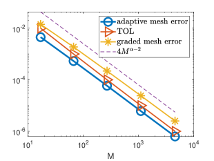
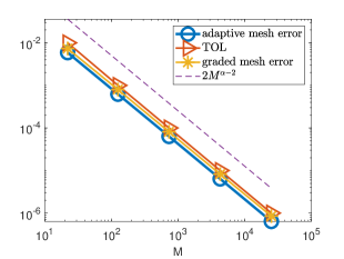
Figure 1: Adaptive algorithm with ${\mathcal{R}}_{0}(t)$ for test problem A: $\max_{[0,T]}|e(t)|$ on the adaptive mesh, the corresponding ${\it TOL}$ and error on the graded mesh, $\alpha=0.4$ (left) and $\alpha=0.7$ (centre). Right: graphs of $\{t_{j}\}_{j=0}^{M}$ as a function of $j/M$ for the adaptive mesh v graded mesh with $r=(2-\alpha)/\alpha$, $\alpha=0.7$, ${\it TOL}=10^{-3}$, $M=67$.

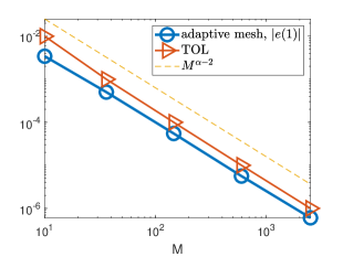
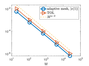
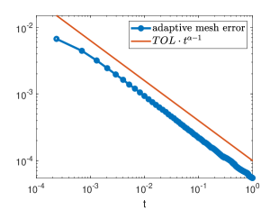
Figure 2: Adaptive algorithm with ${\mathcal{R}}_{1}(t)$ for test problem A: $|e(1)|$ on the adaptive mesh and the corresponding ${\it TOL}$, $\alpha=0.4$ (left) and $\alpha=0.7$ (centre). Right: log-log graph of the pointwise error $|e(t_{j})|$ on the adaptive mesh v ${\it TOL}\cdot t^{\alpha-1}$, $\alpha=0.4$, ${\it TOL}=10^{-4}$, $M=146$.

The errors and rates of convergence obtained using residual barriers ${\mathcal{R}}_{0}(t)$ and ${\mathcal{R}}_{1}(t)$ are presented in Fig. 1 & 2. For ${\mathcal{R}}_{0}$, the errors on the adaptive meshes were compared with the errors on the optimal graded meshes $\{t_{j}=T(j/M)^{r}\}_{j=0}^{M}$ with $r=(2-\alpha)/\alpha$ [5, 8, 12] for the same values of $M$. We observe that in both cases the optimal global rates of convergence $2-\alpha$ are attained. Furthermore, not only the adaptive meshes successfully detect the solution singularity, but they slightly outperform the optimal graded meshes. For ${\mathcal{R}}_{1}$, we observe the optimal rates of convergence $2-\alpha$ at terminal time $t=1$, which is consistent with the error bound [8, (3.2)] for a mildly graded mesh (see Remark 2.6).

4.2 Numerical results for fractional parabolic test problems

Test problem B. Next, we consider (1.1) for $(x,t)\in(0,\pi)\times(0,1]$ with ${\mathcal{L}}=-\partial_{x}^{2}$ and the exact solution $u:=(t^{\alpha}-t^{2})\,\sin(x^{2}/\pi)$, so we set $\lambda:=1$. The same adaptive algorithm was employed with ${\mathcal{R}}_{0}(t)$ from (2.3) to generate temporal meshes, while in space the problem was discretized on the uniform mesh with $10^{4}$ intervals using standard finite differences (equivalent to lumped-mass linear finite elements). The numerical results are given on Fig. 3 (left, centre) are similar to those on Fig. 1 for test problem A.

Test problem C. Our final test is (1.1) for $(x,t)\in(0,\pi)\times(0,0.2]$ with ${\mathcal{L}}=-\partial_{x}^{2}$, so $\lambda:=1$. Now $u_{0}:=x$ for $x\leq 1$ and $u_{0}:=1-(x-1)/(\pi-1)$ for $x\geq 1$, while $f:=0$. As ${\mathcal{L}}u_{0}\not\in L_{2}(\Omega)$, to be able to compute $\|R_{h}\|$ on $(0,t_{1})$, we change the interpolation of the computed solution $\{u_{h}^{j}\}_{j=0}^{M}$ on $(0,t_{1}]$ to piecewise-constant, as described in Remark 2.7. The residual becomes $R_{h}=[u_{h}^{1}-u_{h}^{0}]\{\Gamma(1-\alpha)\}^{-1}t^{-\alpha}+{\mathcal{L}}u_{h}^{1}-f(\cdot,t)$ for $t\in(0,t_{1}]$ and $R_{h}=(D_{t}^{\alpha}u_{h}-f)-(D_{t}^{\alpha}u_{h}-f)^{I}+[u_{h}^{1}-u_{h}^{0}]\{\Gamma(1-\alpha)\}^{-1}\sigma(t)$ for $t>t_{1}$, where $\sigma(t):=t^{-\alpha}-(1-\alpha)^{-1}[t^{1-\alpha}-(t-t_{1})^{1-\alpha}]/t_{1}$. A fixed mesh with $10^{5}$ subintervals was used in space. The reference solution was computed on a finer mesh. The numerical results, given on Fig. 3 (right) indicate that our adaptive algorithm provides adequate error control for piecewise-linear initial data, as well as for more typical solution singularities at initial time. For a further numerical study of this approach, we refer the reader to [3].

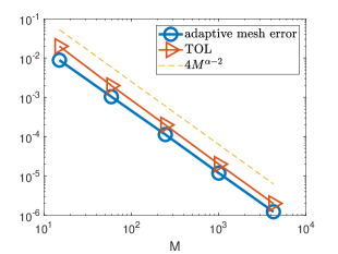
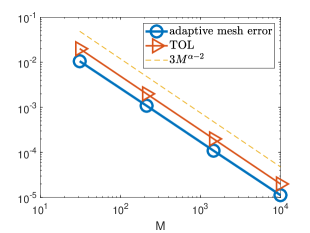
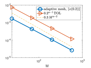
Figure 3: Adaptive algorithm with ${\mathcal{R}}_{0}(t)$ for parabolic test problem B: $\max_{t_{j}\in(0,T]}\|e(t_{j})\|$ on the adaptive mesh and the corresponding ${\it TOL}$, $\alpha=0.4$ (left) and $\alpha=0.8$ (centre). Adaptive algorithm with ${\mathcal{R}}_{0}(t)$ for parabolic test problem C: , $\|e(0.2)\|$ and ${\it TOL}$, $\alpha=0.6$ (right).

4.3 Adaptive algorithm

We employed the algorithm in Fig. 4, with parameters $Q:=1.1$, $\tau_{*}:=5\,{\it TOL}^{1/\alpha}$ for ${\mathcal{R}}_{0}$ and $\tau_{*}:={\it TOL}$ for ${\mathcal{R}}_{1}$, $\tau_{**}:=0$. Here we used the standard mathematical notation combined with the MatLab while loop syntax (where, to be precise, break denotes an exit from the interior while loop).

$u_{h}^{0}:=u_{0}$;  $t_{0}:=0$;  $t_{1}:=\min\{\tau_{*},\,T\}$;  $m:=0$;

while  $t_{m}<T$

$m:=m+1$;  $flag:=0$;

while  $t_{m}-t_{m-1}>\tau_{**}$

compute $u_{h}^{m}$ using (4.1)

if  $\|R_{h}(\cdot,t)\|\leq{\it TOL}\cdot{\mathcal{R}}_{p}(t)$ $\forall\,t\in(t_{m-1},t_{m})$

if  $t_{m}=T$

$M:=m$;  break

elseif  $t_{m}<T$

$\tilde{u}_{h}^{m}:=u_{h}^{m}$;  $\tilde{t}_{m}:=t_{m}$;

$t_{m}:=\min\{t_{m-1}+Q(t_{m}-t_{m-1}),\,T\}$;  $flag:=1$;

end

else

if  $flag=0$

$t_{m}:=t_{m-1}+(t_{m}-t_{m-1})/Q$;

else

$u_{h}^{m}:=\tilde{u}_{h}^{m}$;  $t_{m}:=\tilde{t}_{m}$;

$t_{m+1}:=\min\{t_{m}+(t_{m}-t_{m-1}),\,T\}$;  break

end

end

end

end

Figure 4: Adaptive algorithm.