Kernel Thinning

Abstract

We introduce kernel thinning, a new procedure for compressing a distribution $\mathbb{P}$ more effectively than i.i.d. sampling or standard thinning. Given a suitable reproducing kernel $\mathbf{k}_{\star}$ and $\mathcal{O}(n^{2})$ time, kernel thinning compresses an $n$-point approximation to $\mathbb{P}$ into a $\sqrt{n}$-point approximation with comparable worst-case integration error across the associated reproducing kernel Hilbert space. The maximum discrepancy in integration error is $\mathcal{O}_{d}(n^{-1/2}\sqrt{\log n})$ in probability for compactly supported $\mathbb{P}$ and $\mathcal{O}_{d}(n^{-\frac{1}{2}}(\log n)^{(d+1)/2}\sqrt{\log\log n})$ for sub-exponential $\mathbb{P}$ on $\mathbb{R}^{d}$. In contrast, an equal-sized i.i.d. sample from $\mathbb{P}$ suffers $\Omega(n^{-1/4})$ integration error. Our sub-exponential guarantees resemble the classical quasi-Monte Carlo error rates for uniform $\mathbb{P}$ on $[0,1]^{d}$ but apply to general distributions on $\mathbb{R}^{d}$ and a wide range of common kernels. Moreover, the same construction delivers near-optimal $L^{\infty}$ coresets in $\mathcal{O}(n^{2})$ time. We use our results to derive explicit non-asymptotic maximum mean discrepancy bounds for Gaussian, Matérn, and B-spline kernels and present two vignettes illustrating the practical benefits of kernel thinning over i.i.d. sampling and standard Markov chain Monte Carlo thinning, in dimensions $d=2$ through $100$.

coresets, distribution compression, Markov chain Monte Carlo, maximum mean discrepancy, reproducing kernel Hilbert space, thinningarxiv

1 Introduction

Monte Carlo and Markov chain Monte Carlo (MCMC) methods [14] are commonly used to approximate intractable target expectations $\mathbb{P}f\triangleq{\mathbb{E}}_{X\sim\mathbb{P}}[f(X)]$ of $\mathbb{P}$-integrable functions $f$ with asymptotically exact averages $\mathbb{P}_{n}f\!\triangleq\!\frac{1}{n}\sum_{i=1}^{n}f(x_{i})$ based on points $(x_{i})_{i=1}^{n}$ generated from a Markov chain. A standard practice, to minimize the expense of downstream function evaluation, is to thin the Markov chain output down to a smaller size $n_{\mathrm{out}}$ by keeping only every $({n/}{n_{\mathrm{out}}})$-th sample point [65]. We call this approach standard thinning, and such sample compression is critical in fields like computational cardiology in which each function evaluation triggers an organ or tissue simulation consuming thousands of CPU hours [60, 2, 83]. Unfortunately, standard thinning also leads to a significant reduction in accuracy. For example, thinning one’s chain down to $n_{\mathrm{out}}=\sqrt{n}$ sample points increases integration error from $\mathcal{O}(n^{-\frac{1}{2}})$ in probability to $\Omega(n^{-\frac{1}{4}})$ by the Markov chain central limit theorem [73, Prop. 29]. Our primary contribution is a more effective thinning strategy, which provides $o_{p}(n^{-\frac{1}{4}})$-integration error when $n^{\frac{1}{2}}$ points are returned.

1.1 Thinned MMD coresets

We focus on integration error in a reproducing kernel Hilbert space [RKHS, 81, Def. 4.18] of bounded, measurable functions with a target kernel ${\mathbf{k}_{\star}}:{}^{d}\times{}^{d}\to\real$ for $d\in\mathbb{N}$ and RKHS norm $\|{\cdot}\|_{{\mathbf{k}_{\star}}}$.

Assumption 1 (RKHS of bounded, measurable functions).

The RKHS $\mathcal{H}_{\mathbf{k}}$ of a kernel $\mathbf{k}:{}^{d}\times{}^{d}\to\real$ contains only bounded measurable functions. Equivalently, $\mathbf{k}$ is bounded with $\mathbf{k}(x,\cdot)$ measurable for all $x\in\mathbb{R}^{d}$ [81, Lems. 4.23, 4.24].

The worst-case integration error over the RKHS unit ball is given by the kernel maximum mean discrepancy [MMD, 33].

Definition 1 (Maximum mean discrepancy [33]).

For a kernel $\mathbf{k}$ satisfying Assump. 1, we define the kernel maximum mean discrepancy,

$$\operatorname{MMD}_{\mathbf{k}}(\mu,\nu) \triangleq\sup_{f\in\mathcal{H}_{\mathbf{k}}:\mathopen{}\mathclose{{}\left\|{f}}\right\|_{\mathbf{k}}\leq 1}\mathopen{}\mathclose{{}\left|\mu f-\nu f}\right|\quad\text{for all probability measures $\mu,\nu$ on $\mathbb{R}^{d}$.}\quad$$ (1)

For sequences of points $\mathcal{S}$ and $\mathcal{S}^{\prime}$ in $\mathbb{R}^{d}$ with empirical distributions $\mathbb{Q}$ and $\mathbb{Q}^{\prime}$, we overload this notation to write $\operatorname{MMD}_{\mathbf{k}}(\mathbb{P},\mathcal{S})\triangleq\operatorname{MMD}_{\mathbf{k}}(\mathbb{P},\mathbb{Q})$ and $\operatorname{MMD}_{\mathbf{k}}(\mathcal{S},\mathcal{S}^{\prime})\triangleq\operatorname{MMD}_{\mathbf{k}}(\mathbb{Q},\mathbb{Q}^{\prime})$.

Given ${\mathbf{k}_{\star}}$ satisfying Assump. 1, a target distribution $\mathbb{P}$ on $\mathbb{R}^{d}$, and a sequence of $\mathbb{R}^{d}$-valued points $(x_{i})_{i=1}^{n}$ generated to approximate $\mathbb{P}$, our aim is to identify a thinned MMD coreset, a shorter subsequence that continues to approximate $\mathbb{P}$ well in $\operatorname{MMD}_{\mathbf{k}_{\star}}$.

Definition 2 (MMD coreset).

We call a sequence of $n_{\mathrm{out}}$ points in $\mathbb{R}^{d}$ with empirical measure $\mathbb{Q}$ an $(n_{\mathrm{out}},\varepsilon)$-MMD coreset for $({\mathbf{k}_{\star}},\mathbb{P})$ if $\operatorname{MMD}_{{\mathbf{k}_{\star}}}(\mathbb{P},\mathbb{Q})\leq\varepsilon$.

Notably, when the initial sequence is drawn i.i.d. or from a fast-mixing Markov chain targeting $\mathbb{P}$, standard thinning down to size $n_{\mathrm{out}}=n^{\frac{1}{2}}$ yields an order $(n^{\frac{1}{2}},n^{-\frac{1}{4}})$-MMD coreset in probability (see Prop. 1). A benchmark for improvement is provided by the online Haar strategy of Dwivedi et al. [26], which generates an $(n^{\frac{1}{2}},\mathcal{O}_{d}(n^{-\frac{1}{2}}\log^{2d}n))$-MMD coreset in probability from $2n^{\frac{1}{2}}$ i.i.d. sample points when $\mathbb{P}$ is specifically the uniform distribution on the unit cube $[0,1]^{d}$. Our goal is to develop thinned coresets of improved quality for any target $\mathbb{P}$ with sufficiently fast tail decay.

1.2 Our contributions

To this end, we introduce kernel thinning (Alg. 1), a new, practical solution to the thinned MMD coreset problem that takes as input an $(n,\mathcal{O}_{p}(n^{-\frac{1}{2}}))$-MMD coreset and outputs an $(n^{\frac{1}{2}},o_{p}(n^{-\frac{1}{4}}))$-MMD coreset for a wide-range of $({\mathbf{k}_{\star}},\mathbb{P})$. Kernel thinning uses non-uniform randomness and evaluations of a less smooth square-root kernel ${\mathbf{k}}_{\mathrm{rt}}$ (see Def. 5) to partition the input into subsets of comparable quality and then greedily refines the best of these subsets using ${\mathbf{k}_{\star}}$. Our primary contributions include:

1. Better-than-i.i.d. MMD coresets: Given $n$ input points sampled i.i.d. or from a fast-mixing Markov chain, kernel thinning yields, in probability, an $(n^{\frac{1}{2}},\mathcal{O}_{d}(n^{-\frac{1}{2}}\sqrt{\log n}))$-MMD coreset for $\mathbb{P}$ and ${\mathbf{k}}_{\mathrm{rt}}$ with bounded support, an $(n^{\frac{1}{2}},\mathcal{O}_{d}(n^{-\frac{1}{2}}\sqrt{\log^{d+1}n\log\log n}))$-MMD coreset for $\mathbb{P}$ and ${\mathbf{k}}_{\mathrm{rt}}$ with light tails, and an $(n^{\frac{1}{2}},\mathcal{O}_{d}(n^{-\frac{1}{2}+\frac{d}{2\rho}}\sqrt{\log n\log\log n}))$-MMD coreset for $\mathbb{P}$ and ${\mathbf{k}}_{\mathrm{rt}}^{2}$ with $\rho>2d$ moments (Thms. 1 and 1). For compactly supported or light-tailed $\mathbb{P}$ and ${\mathbf{k}}_{\mathrm{rt}}$, these results compare favorably with known $\Omega_{d}(n^{-\frac{1}{2}})$ lower bounds (see Sec. 8.1). Our guarantees extend to more general input point sequences, including deterministic sequences based on quadrature or kernel herding [20], and give rise to explicit, non-asymptotic error bounds for a wide variety of popular kernels including Gaussian, Matérn, and B-spline kernels. While $(n^{\frac{1}{2}},\mathcal{O}_{d}(n^{-\frac{1}{2}}\log^{\frac{d-1}{2}}n))$-MMD coresets have been developed for specific $({\mathbf{k}_{\star}},\mathbb{P})$ pairings like the uniform distribution on $[0,1]^{d}$ and an $L^{2}$ discrepancy kernel ${\mathbf{k}_{\star}}$ (see Sec. 8.1), to the best of our knowledge, no prior $(n^{\frac{1}{2}},o_{p}(n^{-\frac{1}{4}}))$-MMD coreset constructions were known for the range of $\mathbb{P}$ and ${\mathbf{k}_{\star}}$ studied in this work.

2. MMD error from square-root $L^{\infty}$ error: To derive our MMD guarantees for kernel thinning, we first establish an important link between MMD coresets for ${\mathbf{k}_{\star}}$ and $L^{\infty}$ coresets for ${\mathbf{k}}_{\mathrm{rt}}$.

   Definition 3 ($L^{\infty}$ coreset).

   For any kernel $\mathbf{k}$ satisfying Assump. 1, probability measure $\mu$ on $\mathbb{R}^{d}$, and $z\in\mathbb{R}^{d}$, let $\mu\mathbf{k}(z)\triangleq\mathbb{E}_{X\sim\mu}[\mathbf{k}(X,z)]$. We call a sequence of $n_{\mathrm{out}}$ points in $\mathbb{R}^{d}$ with empirical measure $\mathbb{Q}$ an $(n_{\mathrm{out}},\varepsilon)$-$L^{\infty}$ coreset for $(\mathbf{k},\mathbb{P})$ if $\|\mathbb{P}\mathbf{k}-\mathbb{Q}\mathbf{k}\|_{\infty}\leq\varepsilon$.

   Thms. 2 and 2 show that any $L^{\infty}$ coreset for $({\mathbf{k}}_{\mathrm{rt}},\mathbb{P})$ is also an MMD coreset for $({\mathbf{k}_{\star}},\mathbb{P})$ with quality depending on the tail decay of ${\mathbf{k}}_{\mathrm{rt}}$ and $\mathbb{P}$.

3. Online vector balancing in Hilbert spaces: As a building block for constructing high-quality coresets, we introduce and analyze a Hilbert space generalization of the self-balancing walk of Alweiss et al. [1] to partition a sequence of functions (like $({\mathbf{k}}_{\mathrm{rt}}(x_{i},\cdot))_{i=1}^{n}$) into nearly equal halves. Our analysis of this self-balancing Hilbert walk (SBHW, Alg. 5) in Thm. 3 may be of independent interest for solving the online vector balancing problem of Spencer [79] in Hilbert spaces (Cor. 4).

4. Efficient, near-optimal $L^{\infty}$ coresets: We then design a symmetrized version of SBHW for RKHSes—kernel halving—that delivers $2$-thinned coresets with small $L^{\infty}$ error (Algs. 3 and 4). The first stage of kernel thinning, [algo:ktsplit]kt-split, recursively applies kernel halving to ${\mathbf{k}}_{\mathrm{rt}}$ to obtain near-minimax-optimal $L^{\infty}$ coresets in $\mathcal{O}(n^{2})$ time with $\mathcal{O}(n\min(d,n))$ space (Cors. 5 and 6).

After describing our kernel and input point requirements in Sec. 2, we detail the kernel thinning and kernel halving algorithms in Sec. 3. Sec. 4 houses our main MMD guarantees, both for kernel thinning and for generic $L^{\infty}$ square-root kernel coresets. We introduce and analyze the self-balancing Hilbert walk in Sec. 5 and present our main $L^{\infty}$ guarantees for kernel halving and [algo:ktsplit]kt-split in Sec. 6. Sec. 7 complements our theoretical contributions with two vignettes illustrating the practical benefits of kernel thinning over (a) i.i.d. sampling in dimensions $d=2$ through $100$ and (b) standard MCMC thinning across twelve experiments targeting challenging differential equation posterior distributions. We conclude with a discussion of our results, related work, and future directions in Sec. 8 and defer all proofs to the appendices.

Notation

We define the shorthand $[n]\triangleq\{1,\dots,n\}$ for $n\in\mathbb{N}$, $a\wedge b\triangleq\min(a,b)$ for $a,b\in\mathbb{R}$, ${}_{+}\triangleq\mathopen{}\mathclose{{}\left\{x\in\real:x\geq 0}\right\}$, and $\mathcal{B}(x;r)\triangleq\mathopen{}\mathclose{{}\left\{y\in\mathbb{R}^{d}\mid\mathopen{}\mathclose{{}\left\|{x-y}}\right\|_{2}<r}\right\}$ for $r\in\mathbb{R}$. We use $\mathrm{Vol}(\mathcal{B})$ to denote the volume of a compact set $\mathcal{B}\subset{}^{d}$. We let $\mathcal{A}^{c}$ denote the complement of a set $\mathcal{A}\subset\mathbb{R}^{d}$ and $\mathbb{I}_{\mathcal{A}}(x)=1$ if $x\in\mathcal{A}$ and 0 otherwise. We use $\mathrm{Pr}(\mathcal{E})$ to denote the probability of an event $\mathcal{E}$. For real-valued kernels $\mathbf{k}$ and functions $f$ on $\mathbb{R}^{d}$, we make frequent use of the norms $\mathopen{}\mathclose{{}\left\|{\mathbf{k}}}\right\|_{\infty}=\sup_{x,y\in\mathbb{R}^{d}}|\mathbf{k}(x,y)|$ and $\mathopen{}\mathclose{{}\left\|{f}}\right\|_{\infty}=\sup_{x\in\mathbb{R}^{d}}|f(x)|$. For $x>0$, we use $\Gamma(x)=\int_{0}^{\infty}t^{x-1}e^{-t}\,dt$ to denote the Gamma function (with $\Gamma(n)=(n-1)!$ for $n\in\mathbb{N}$).

For two sequences of real numbers $(a_{n})_{n\in\mathbb{N}}$ and $(b_{n})_{n\in\mathbb{N}}$, we say that $a_{n}$ is of order $b_{n}$ and write $a_{n}=\mathcal{O}(b_{n})$ or $a_{n}\precsim b_{n}$ to denote that $a_{n}\leq cb_{n}$ for all $n\in\mathbb{N}$ and some constant $c>0$. We write $a_{n}=\Omega(b_{n})$ if $b_{n}=\mathcal{O}(a_{n})$ and $a_{n}=\Theta(b_{n})$ when $a=\Omega(b_{n})$ and $a=\mathcal{O}(b_{n})$. Moreover, we use $a_{n}=\mathcal{O}_{d}(b_{n}),a_{n}\precsim_{d}b_{n},a_{n}=\Omega_{d}(b_{n}),a_{n}\succsim_{d}b_{n}$ to indicate dependency of underlying universal constant on $d$. We say $a_{n}=o(b_{n})$ if $\lim_{n\to\infty}a_{n}/b_{n}=0$. For a sequence of real-valued random variables $(X_{n})_{n\in\mathbb{N}}$, we write $X_{n}=\mathcal{O}_{P}(a_{n})$ or $X_{n}=\mathcal{O}(a_{n})$ in probability, when $\frac{X_{n}}{a_{n}}$ is stochastically bounded, i.e., for all $\delta>0$, there exists finite $c_{\delta}$ and $n_{\delta}$ such that $\mathrm{Pr}(|\frac{X_{n}}{a_{n}}|>c_{\delta})<\delta$, for all $n>n_{\delta}$. We write $X_{n}=\Omega_{P}(a_{n})$ if $1/X_{n}=\mathcal{O}_{P}(1/b_{n})$ and $X_{n}=o_{p}(a_{n})$ when $\frac{X_{n}}{a_{n}}\to 0$ in probability, i.e., for all $\varepsilon>0$, $\mathrm{Pr}(|\frac{X_{n}}{a_{n}}|\geq\varepsilon)\to 0$.

We write order $(n,\varepsilon)$-MMD (or $L^{\infty}$) coreset to mean an $(n,\mathcal{O}(\epsilon))$-MMD (or $L^{\infty}$) coreset and append in probability to mean an $(n,\mathcal{O}_{p}(\epsilon))$-MMD (or $L^{\infty}$) coreset.

2 Input Point and Kernel Requirements

Given a target distribution $\mathbb{P}$ on $\mathbb{R}^{d}$, a kernel ${\mathbf{k}_{\star}}$ satisfying Assump. 1, and a sequence of $\mathbb{R}^{d}$-valued input points $\mathcal{S}_{n}\!=\!(x_{i})_{i=1}^{n}$ generated either randomly or deterministically, our goal is to identify a better-than-i.i.d. thinned MMD coreset, that is, a subsequence $\mathcal{S}_{\mathrm{out}}$ of size $n^{\frac{1}{2}}$ satisfying $\operatorname{MMD}_{\mathbf{k}_{\star}}(\mathbb{P},\mathcal{S}_{\mathrm{out}})\!=\!o_{p}(n^{-\frac{1}{4}})$. When drawing asymptotic conclusions, we will view $d$ as fixed and $\mathcal{S}_{n}$ as a prefix of an infinite sequence of points $\mathcal{S}_{\infty}\triangleq(x_{i})_{i=1}^{\infty}$.

2.1 Input point requirements

Our algorithms are designed to return high quality MMD coresets for the input $\mathcal{S}_{n}$. To translate these into high quality coresets for the target $\mathbb{P}$, it suffices, by the triangle inequality, for the input points to have quality $\operatorname{MMD}_{{\mathbf{k}_{\star}}}(\mathbb{P},\mathcal{S}_{n})=\mathcal{O}_{p}(n^{-\frac{1}{2}})$. As we discuss in Sec. 8.1, input sequences generated by i.i.d. sampling, kernel herding [20], Stein Point MCMC [19], and greedy sign selection [46] all satisfy this property. Moreover, we prove in App. B that an analogous guarantee holds for the iterates of a fast-mixing Markov chain.

Proposition 1 (MMD guarantee for MCMC).

Consider a homogeneous $\phi$-irreducible geometrically ergodic Markov chain [28, Thm. 1xi] with initial state $x_{0}$, subsequent iterates $\mathcal{S}_{\infty}$, and stationary distribution $\mathbb{P}$. If ${\mathbf{k}_{\star}}$ satisfies Assump. 1, then there exists a $\mathbb{P}$-almost everywhere finite function $c:\mathbb{R}^{d}\to(0,\infty]$ such that, for any given $n\in\mathbb{N}$ and $\delta\in(0,1)$, $\operatorname{MMD}_{{\mathbf{k}_{\star}}}(\mathbb{P},\mathcal{S}_{n})\leq\sqrt{\frac{c(x_{0})\mathopen{}\mathclose{{}\left\|{{\mathbf{k}_{\star}}}}\right\|_{\infty}\log(e/\delta)}{n}}$ with probability $1-\delta$ given $x_{0}$.

The input radius,

$$\textstyle R_{\mathcal{S}_{n}}\!\triangleq\!\max_{x\in\mathcal{S}_{n}}\mathopen{}\mathclose{{}\left\|{x}}\right\|_{2},$$ (2)

will also play an important role in our results. In particular, the growth rate of this radius as a function of $n$ impacts the growth rate of our MMD bounds. Our next definition assigns familiar names to the most commonly encountered growth rates.

Definition 4 (Input radius growth rates).

We say the point sequence $\mathcal{S}_{\infty}$ with prefixes $\mathcal{S}_{n}$ for $n\in\mathbb{N}$ is Compact if $R_{\mathcal{S}_{n}}=\mathcal{O}_{d}(1)$, SubGauss if $R_{\mathcal{S}_{n}}=\mathcal{O}_{d}(\sqrt{\log n})$, SubExp if $R_{\mathcal{S}_{n}}=\mathcal{O}_{d}(\log n)$, and $\textsc{HeavyTail}(\rho)$ with $\rho>0$ if $R_{\mathcal{S}_{n}}=\mathcal{O}_{d}(n^{1/\rho})$.

These growth rates are exactly those which arise with probability $1$ when an input sequence is generated identically from $\mathbb{P}$ with corresponding tail behavior or from a fast-mixing Markov chain targeting $\mathbb{P}$. Our proof of this result is given in App. C.

Proposition 2 (Almost sure radius growth).

Suppose that the points $x_{0}$ and $\mathcal{S}_{\infty}$ are either (i) sampled identically (but not necessarily independently) from $\mathbb{P}$ or (ii) the iterates of a homogeneous $\phi$-irreducible geometrically ergodic Markov chain with initial state $x_{0}$, subsequent iterates $\mathcal{S}_{\infty}$, and stationary distribution $\mathbb{P}$. Then the following statements hold true for any nonnegative $c$ and $\rho$ and $\mathbb{P}$-almost every $x_{0}$.

1. If $\mathbb{P}$ is compactly supported, then, with probability $1$ conditional on $x_{0}$, $\mathcal{S}_{\infty}$ is Compact.

2. If $\mathbb{E}_{X\sim\mathbb{P}}[e^{c\mathopen{}\mathclose{{}\left\|{X}}\right\|_{2}^{2}}]<\infty$, then, with probability $1$ conditional on $x_{0}$, $\mathcal{S}_{\infty}$ is SubGauss.

3. If $\mathbb{E}_{X\sim\mathbb{P}}[e^{c\mathopen{}\mathclose{{}\left\|{X}}\right\|_{2}}]<\infty$, then, with probability $1$ conditional on $x_{0}$, $\mathcal{S}_{\infty}$ is SubExp.

4. If $\mathbb{E}_{X\sim\mathbb{P}}[\mathopen{}\mathclose{{}\left\|{X}}\right\|_{2}^{\rho}]<\infty$, then, with probability $1$ conditional on $x_{0}$, $\mathcal{S}_{\infty}$ is $\textsc{HeavyTail}(\rho)$.

Finally, we will also require $\mathcal{S}_{\infty}$ to be oblivious, that is, generated independently of any randomness in the thinning algorithm. To capture this assumption, we treat $\mathcal{S}_{\infty}$ as fixed and deterministic hereafter. This treatment is without loss of generality since our results hold conditional on the observed values of $(x_{i})_{i=1}^{\infty}$ when the points are random and oblivious.

2.2 Kernel requirements

We use the terms reproducing kernel and kernel interchangeably to indicate that ${\mathbf{k}_{\star}}$ is symmetric and positive definite, i.e., that the kernel matrix $({\mathbf{k}_{\star}}(z_{i},z_{j}))_{i,j=1}^{l}$ is symmetric and positive semidefinite for any evaluation points $(z_{i})_{i=1}^{l}$ in $\mathbb{R}^{d}$. In addition to ${\mathbf{k}_{\star}}$, our algorithm takes as input a square-root kernel for ${\mathbf{k}_{\star}}$.

Definition 5 (Square-root kernel).

We say a kernel ${\mathbf{k}}_{\mathrm{rt}}:\mathbb{R}^{d}\times\mathbb{R}^{d}\to\mathbb{R}$ is a square-root kernel for ${\mathbf{k}_{\star}}:\mathbb{R}^{d}\times\mathbb{R}^{d}\to\mathbb{R}$ if ${\mathbf{k}}_{\mathrm{rt}}(x,\cdot)$ is square integrable for all $x\in\mathbb{R}^{d}$ with

$$\textstyle{\mathbf{k}_{\star}}(x,y)=\int_{\mathbb{R}^{d}}{\mathbf{k}}_{\mathrm{rt}}(x,z){\mathbf{k}}_{\mathrm{rt}}(y,z)dz\quad\text{for all}\quad x,y\in{}^{d}.$$ (3)

We highlight that a square-root kernel need not be unique and that its existence is an indication of a certain degree of smoothness in the target kernel ${\mathbf{k}_{\star}}$. One convenient tool for deriving square-root kernels is the notion of a spectral density.

Definition 6 (Shift invariance and spectral density).

We call a kernel of the form $\mathbf{k}(x,y)=\kappa(x-y)$ for $\kappa:\mathbb{R}^{d}\to\mathbb{R}$ shift-invariant and say $\mathbf{k}$ has spectral density $\widehat{\kappa}$ if $\kappa$ is the Fourier transform of a finite measure with Lebesgue density $\widehat{\kappa}$, i.e., $\kappa(z)=\frac{1}{(2\pi)^{d/2}}\int e^{-i\langle{\omega},{z}\rangle}\widehat{\kappa}(\omega)d\omega$.

Name of kernel
${\mathbf{k}_{\star}}(x,y)=\kappa(x\!-\!y)$	Expression for
$\kappa(z)$	Fourier transform
$\widehat{\kappa}(\omega)$	Square-root kernel
${\mathbf{k}}_{\mathrm{rt}}$
Gaussian$(\sigma):$
$\sigma>0$	$\exp\mathopen{}\mathclose{{}\left(-\frac{\mathopen{}\mathclose{{}\left\|{z}}\right\|_{2}^{2}}{2\sigma^{2}}}\right)$	$\sigma^{d}\exp\mathopen{}\mathclose{{}\left(-\frac{\sigma^{2}\mathopen{}\mathclose{{}\left\|{\omega}}\right\|_{2}^{2}}{2}}\right)$	$\mathopen{}\mathclose{{}\left(\frac{2}{\pi\sigma^{2}}}\right)^{\frac{d}{4}}\textbf{Gaussian}\mathopen{}\mathclose{{}\left(\frac{\sigma}{\sqrt{2}}}\right)$
Matérn$(\nu,\gamma):$
$\nu>d,\gamma>0$	$c_{\nu-\frac{d}{2}}(\gamma\mathopen{}\mathclose{{}\left\|{z}}\right\|_{2})^{\nu-\frac{d}{2}}{K}_{\nu-\frac{d}{2}}(\gamma\mathopen{}\mathclose{{}\left\|{z}}\right\|_{2})$	${\phi_{d,\nu,\gamma}\,}{(\gamma^{2}+\mathopen{}\mathclose{{}\left\|{\omega}}\right\|_{2}^{2})^{-\nu}}$	$A_{\nu,\gamma,d}$Matérn$(\frac{\nu}{2},\gamma)$
$\textbf{B-spline}(2\beta+1):$
$\beta\in 2\mathbb{N}+1$	$S_{2\beta+2,d}\displaystyle\prod_{j=1}^{d}\circledast^{2\beta+2}\mathbb{I}_{[-\frac{1}{2},\frac{1}{2}]}(z_{j})$	$S_{2\beta+2,d}^{\prime}\displaystyle\prod_{j=1}^{d}{\textstyle\frac{\sin^{2\beta+2}(\frac{\omega_{j}}{2})}{\omega_{j}^{2\beta+2}}}$	$\widetilde{S}_{\beta,d}\textbf{B-spline}(\beta)$

arxiv jmlr

Table 1: Square-root kernels ${\mathbf{k}}_{\mathrm{rt}}$ for common target kernels ${\mathbf{k}_{\star}}$. Each ${\mathbf{k}_{\star}}$ satisfies $\mathopen{}\mathclose{{}\left\|{{\mathbf{k}_{\star}}}}\right\|_{\infty}=1$, and the parameter range ensures the existence of ${\mathbf{k}}_{\mathrm{rt}}$. Above, $\circledast^{\ell}$ denotes recursive convolution with $\ell$ function copies, ${K}_{a}$ denotes the modified Bessel function of the third kind [91, Def. 5.10], $c_{b}\triangleq\frac{2^{1-b}}{\Gamma(b)}$, $\phi_{d,\nu,\gamma}=\frac{c_{\nu-d/2}}{c_{\nu}}\gamma^{2\nu-d}$, $A_{\nu,\gamma,d}\triangleq\mathopen{}\mathclose{{}\left(\frac{1}{4\pi}\gamma^{2}}\right)^{d/4}\sqrt{\frac{\Gamma(\nu)}{\Gamma(\nu-d/2)}}\cdot\frac{\Gamma((\nu-d)/2)}{\Gamma(\nu/2)}$, $S_{2\beta+2,d}^{\prime}\triangleq S_{2\beta+2,d}\cdot(\frac{4^{\beta+1}}{\sqrt{2\pi}})^{d}$, and $\widetilde{S}_{\beta,d}\triangleq\frac{\sqrt{S_{2\beta+2,d}}}{S_{\beta+1,d}}$ where $S_{\beta,d}$ is defined in 264. See App. N for our derivation.

Table 2: Square-root kernels ${\mathbf{k}}_{\mathrm{rt}}$ for common target kernels ${\mathbf{k}_{\star}}$. Each ${\mathbf{k}_{\star}}$ satisfies $\mathopen{}\mathclose{{}\left\|{{\mathbf{k}_{\star}}}}\right\|_{\infty}=1$, and the parameter range ensures the existence of ${\mathbf{k}}_{\mathrm{rt}}$. Above, $\circledast^{\ell}$ denotes recursive convolution with $\ell$ function copies, ${K}_{a}$ denotes the modified Bessel function of the third kind [91, Def. 5.10], $c_{b}\triangleq\frac{2^{1-b}}{\Gamma(b)}$, $\phi_{d,\nu,\gamma}=\frac{c_{\nu-d/2}}{c_{\nu}}\gamma^{2\nu-d}$, $A_{\nu,\gamma,d}\triangleq\mathopen{}\mathclose{{}\left(\frac{1}{4\pi}\gamma^{2}}\right)^{d/4}\sqrt{\frac{\Gamma(\nu)}{\Gamma(\nu-d/2)}}\cdot\frac{\Gamma((\nu-d)/2)}{\Gamma(\nu/2)}$, $S_{2\beta+2,d}^{\prime}\triangleq S_{2\beta+2,d}\cdot(\frac{4^{\beta+1}}{\sqrt{2\pi}})^{d}$, and $\widetilde{S}_{\beta,d}\triangleq\frac{\sqrt{S_{2\beta+2,d}}}{S_{\beta+1,d}}$ where $S_{\beta,d}$ is defined in 264. See App. N for our derivation.

As we show in Apps. N and Q, many familiar kernels admit spectral densities, including Gaussian, Matérn, B-spline, inverse multiquadric, sech, and Wendland’s compactly supported kernels. Moreover, by Bochner’s theorem [10, 91, Thm. 6.6] and the Fourier inversion theorem [91, Cor. 5.24], any continuous ${\mathbf{k}_{\star}}(x,y)=\kappa(x-y)$ with absolutely integrable $\kappa$ has a spectral density equal to the Fourier transform of $\kappa$. Our next result (proved in App. D) derives a square-root kernel for any shift-invariant ${\mathbf{k}_{\star}}$ with a square-root integrable spectral density.

Proposition 3 (Shift-invariant square-root kernels).

If a kernel ${\mathbf{k}_{\star}}(x,y)\!=\!\kappa(x\!-\!y)$ admits a spectral density (Def. 6) $\widehat{\kappa}$ with $\int\sqrt{\widehat{\kappa}(\omega)}d\omega\!<\!\infty$, then ${\mathbf{k}}_{\mathrm{rt}}(x,y)\!=\!\frac{{\kappa}_{\mathrm{rt}}(x-y)}{(2\pi)^{d/4}}$ is a square-root kernel of ${\mathbf{k}_{\star}}$ for ${\kappa}_{\mathrm{rt}}$ the Fourier transform of $\sqrt{\widehat{\kappa}}$.

Tab. 2 gives several examples of common kernels satisfying the conditions of Prop. 3 along with their associated square-root kernels. For example, if ${\mathbf{k}_{\star}}$ is Gaussian with bandwidth $\sigma$, then a rescaled Gaussian kernel with bandwidth $\frac{\sigma}{\sqrt{2}}$ is a valid choice for ${\mathbf{k}}_{\mathrm{rt}}$. For simplicity, our results in the sequel assume the use of an exact square-root kernel ${\mathbf{k}}_{\mathrm{rt}}$, but, as we detail in App. Q, it suffices to use the square-root of any kernel that dominates ${\mathbf{k}_{\star}}$ in the positive-definite order (see Def. 8). For example, we show in Prop. 4 of App. Q that a standard Matérn kernel is a suitable square-root dominating kernel for any sufficiently-smooth shift-invariant ${\mathbf{k}_{\star}}$ with absolutely integrable $\kappa$. In Tab. 10 of App. Q, we also derive convenient tailored square-root dominating kernels for inverse multiquadric, sech, and Wendland’s compactly supported kernels.

Finally, we define several kernel growth and decay properties that will be explicitly assumed in some of our results.

Assumption 2 (Lipschitz kernel).

The kernel $\mathbf{k}:\mathbb{R}^{d}\times\mathbb{R}^{d}\to\mathbb{R}$ admits a Lipschitz constant

$$\textstyle L_{\mathbf{k}}\triangleq\sup_{x,y,z}\frac{\mathopen{}\mathclose{{}\left|\mathbf{k}(x,y)-\mathbf{k}(x,z)}\right|}{\mathopen{}\mathclose{{}\left\|{y-z}}\right\|_{2}}<\infty.$$ (4)

Assumption 3 (Kernel tail decay).

The kernel $\mathbf{k}$ satisfies Assump. 1 and, for each $\varepsilon>0$,

$$\textstyle\begin{split}\textstyle&\textstyle\max\{\ \inf\{r:\sup_{\begin{subarray}{c}x,y:\\ \mathopen{}\mathclose{{}\left\|{x-y}}\right\|_{2}\geq r\end{subarray}}\mathopen{}\mathclose{{}\left|\mathbf{k}(x,y)}\right|\leq\varepsilon\},\quad\inf\{r:\tau_{\mathbf{k}}(r)\leq\varepsilon\}\ \}<\infty,\\ \textstyle&\textstyle\quad\text{where}\quad\tau_{\mathbf{k}}(r)\triangleq(\sup_{x}\int_{\mathopen{}\mathclose{{}\left\|{y}}\right\|_{2}\geq r}\mathbf{k}^{2}(x,x-y)dy)^{\frac{1}{2}}\quad\text{for}\quad r\geq 0.\end{split}$$ (5)

The following definition gives familiar names to commonly encountered tail decay rates.

Definition 7 (Kernel tail decay rate).

For a kernel $\mathbf{k}$ satisfying Assump. 3, define

$$\textstyle\begin{split}\textstyle R_{\mathbf{k},n}&\textstyle\triangleq\inf\{r:\sup_{\begin{subarray}{c}x,y:\\ \mathopen{}\mathclose{{}\left\|{x-y}}\right\|_{2}\geq r\end{subarray}}|\mathbf{k}(x,y)|\leq\frac{\mathopen{}\mathclose{{}\left\|{\mathbf{k}}}\right\|_{\infty}}{n}\},\quad R_{\mathbf{k},n}^{\prime}\triangleq\inf\{r:\tau_{\mathbf{k}}(r)\leq\frac{\mathopen{}\mathclose{{}\left\|{\mathbf{k}}}\right\|_{\infty}}{\sqrt{n}}\},\\ \textstyle\quad\text{and}\quad R_{\mathbf{k},n}^{\dagger}&\textstyle\triangleq\max\{R_{\mathbf{k},n},R_{\mathbf{k},n}^{\prime}\}\end{split}$$ (6)

for $\tau_{\mathbf{k}}$ defined in 5. We say $\mathbf{k}$ is (a) Compact if $R_{\mathbf{k},n}^{\dagger}=\mathcal{O}_{d}(1)$, (b) SubGauss if $R_{\mathbf{k},n}^{\dagger}=\mathcal{O}_{d}(\sqrt{\log n})$, (c) SubExp if $R_{\mathbf{k},n}^{\dagger}=\mathcal{O}_{d}(\log n)$, (d) $\textsc{HeavyTail}(\rho)$ for $\rho>0$ if $R_{\mathbf{k},n}^{\dagger}=\mathcal{O}_{d}(n^{1/\rho})$, and (e) SubPoly if $\log R_{\mathbf{k},n}^{\dagger}=\mathcal{O}_{d}(\log n)$. Notably, any Compact, SubGauss, SubExp, or $\textsc{HeavyTail}(\rho)$ $\mathbf{k}$ is also SubPoly.

Remark 1 (${\mathbf{k}}_{\mathrm{rt}}$ tail decay implies ${\mathbf{k}_{\star}}$ boundedness).

If ${\mathbf{k}}_{\mathrm{rt}}$ satisfying Assump. 3 is a square-root kernel of ${\mathbf{k}_{\star}}$, then there exists a finite $r$ for which ${\mathbf{k}_{\star}}(x,x)=\int{\mathbf{k}}_{\mathrm{rt}}^{2}(x,x-y)dy\leq\|{\mathbf{k}}_{\mathrm{rt}}\|_{\infty}^{2}\mathrm{Vol}(\mathcal{B}(0;r))+\tau_{{\mathbf{k}}_{\mathrm{rt}}}^{2}(r)<\infty$.

Popular examples of Compact, SubGauss, and SubExp $\mathbf{k}$ are B-spline, Gaussian, and Matérn kernels respectively (see Tab. 4). Moreover, one can directly verify that an inverse multiquadric $\mathbf{k}(x,y)=(\gamma^{2}+\mathopen{}\mathclose{{}\left\|{x\!-\!y}}\right\|_{2}^{2})^{-\nu}$ with $\gamma>0$ and $\nu>\frac{d}{4}$ is HeavyTail ​($2\nu\wedge(4\nu\!-\!d)$).

3 Kernel Thinning

Our solution to the thinned coreset problem is kernel thinning, described in Alg. 1. Given a thinning parameter $m\in\mathbb{N}$, kernel thinning proceeds in two stages: [algo:ktsplit]kt-split and [algo:ktswap]kt-swap.

Input: kernels (${\mathbf{k}_{\star}}$,${\mathbf{k}}_{\mathrm{rt}}$), input points $\mathcal{S}_{n}\!=\!(x_{i})_{i=1}^{n}$, thinning parameter $m\in\mathbb{N}$, probabilities $(\delta_{i})_{i=1}^{\lfloor{\frac{n}{2}}\rfloor}$

$(\mathcal{S}^{(m,\ell)})_{\ell=1}^{2^{m}}\leftarrow$ [algo:ktsplit]kt-split $({\mathbf{k}}_{\mathrm{rt}},\mathcal{S}_{n},m,(\delta_{i})_{i=1}^{\lfloor{\frac{n}{2}}\rfloor})$    /​/ Split $\mathcal{S}_{n}$ into $2^{m}$ candidate coresets of size $\lfloor{\frac{n}{2^{m}}}\rfloor$

[2pt] $\ \mathcal{S}_{\mathrm{KT}}\quad\quad\ \ \leftarrow$ [algo:ktswap]kt-swap $({\mathbf{k}_{\star}},\mathcal{S}_{n},(\mathcal{S}^{(m,\ell)})_{\ell=1}^{2^{m}})$  /​/ Select best coreset and iteratively refine

return coreset $\mathcal{S}_{\mathrm{KT}}$ of size $\lfloor{n/2^{m}}\rfloor$

Algorithm 1 Kernel Thinning – Return coreset of size $\lfloor{n/2^{m}}\rfloor$ with small $\operatorname{MMD}_{{\mathbf{k}_{\star}}}$

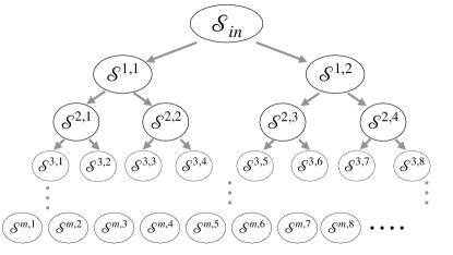
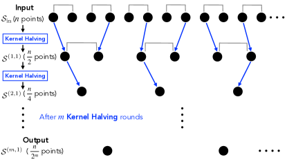
Figure 1: Overview of [algo:ktsplit]kt-split. (Left) [algo:ktsplit]kt-split recursively partitions its input $\mathcal{S}_{n}$ into $2^{m}$ balanced coresets $\mathcal{S}^{(m,\ell)}$ of size $\lfloor{\frac{n}{2^{m}}}\rfloor$. (Right) In Sec. 6, we interpret each coreset $\mathcal{S}^{(m,\ell)}$ as the output of repeated kernel halving: on each halving round, remaining points are paired, and one point from each pair is selected using non-uniform randomness.

Input: kernel ${\mathbf{k}}_{\mathrm{rt}}$, point sequence $\mathcal{S}_{n}=(x_{i})_{i=1}^{n}$, thinning parameter $m\in\mathbb{N}$, probabilities $(\delta_{i})_{i=1}^{\lfloor{n/2}\rfloor}$

$\mathcal{S}^{(j,\ell)}\leftarrow\mathopen{}\mathclose{{}\left\{}\right\}$ for $0\leq j\leq m$ and $1\leq\ell\leq 2^{j}$ // Empty coresets: $\mathcal{S}^{(j,\ell)}$ has size $\lfloor{\frac{i}{2^{j-1}}}\rfloor$ after $i$ rounds

$\sigma_{j,\ell}\leftarrow 0$ for $1\leq j\leq m$ and $1\leq\ell\leq 2^{j-1}$ // Swapping parameters

for $i=1,\ldots,\lfloor{n/2}\rfloor$ do

       $\mathcal{S}^{(0,1)}\texttt{.append}(x_{2i-1});\mathcal{S}^{(0,1)}\texttt{.append}(x_{2i})$

      [2pt] // Every $2^{j-1}$ rounds add point from parent coreset $\mathcal{S}^{(j\!-\!1,\ell)}$ to each child $\mathcal{S}^{(j,2\ell\!-\!1)}$, $\mathcal{S}^{(j,2\ell)}$

      [1pt] for ($j=1;\ j\leq m\ \textbf{and}\ i/2^{j-1}\in\mathbb{N};\ j=j+1$) do

             for $\ell=1,\ldots,2^{j-1}$ do

                   $(\mathcal{S},\mathcal{S}^{\prime})\leftarrow(\mathcal{S}^{(j-1,\ell)},\mathcal{S}^{(j,2\ell-1)})$;  $(x,x^{\prime})\leftarrow\texttt{get\_last\_two\_points}(\mathcal{S})$

                  [2pt] // Compute swapping threshold $\mathfrak{a}$

                  [1pt] $\mathfrak{a},\sigma_{j,\ell}\leftarrow$get_swap_params($\sigma_{j,\ell},\mathfrak{b},\delta_{|{\mathcal{S}}|/2}\cdot\frac{2^{j-1}}{m}$) ​for $\mathfrak{b}^{2}\!=\!{\mathbf{k}}_{\mathrm{rt}}(x,x)\!+\!{\mathbf{k}}_{\mathrm{rt}}(x^{\prime},x^{\prime})\!-\!2{\mathbf{k}}_{\mathrm{rt}}(x,x^{\prime})$

                  [2pt] // Assign one point to each child after probabilistic swapping

                  [1pt] $\alpha\leftarrow{\mathbf{k}}_{\mathrm{rt}}(x^{\prime},x^{\prime})\!-\!{\mathbf{k}}_{\mathrm{rt}}(x,x)+\Sigma_{y\in\mathcal{S}}({\mathbf{k}}_{\mathrm{rt}}(y,x)-{\mathbf{k}}_{\mathrm{rt}}(y,x^{\prime}))\!-\!2\Sigma_{z\in\mathcal{S}^{\prime}}({\mathbf{k}}_{\mathrm{rt}}(z,x)\!-\!{\mathbf{k}}_{\mathrm{rt}}(z,x^{\prime}))$

                  [2pt] $(x,x^{\prime})\leftarrow(x^{\prime},x)$ with probability $\min(1,\frac{1}{2}(1-\frac{\alpha}{\mathfrak{a}})_{+})$

                  [2pt] $\mathcal{S}^{(j,2\ell-1)}\texttt{.append}(x);\quad\mathcal{S}^{(j,2\ell)}\texttt{.append}(x^{\prime})$

             end for

            

       end for

      

end for

return $(\mathcal{S}^{(m,\ell)})_{\ell=1}^{2^{m}}$, candidate coresets of size $\lfloor{n/2^{m}}\rfloor$

function get_swap_params($\sigma,\mathfrak{b},\delta$):

       $\mathfrak{a}\leftarrow\max(\mathfrak{b}\sigma\sqrt{\smash[b]{2\log(2/\delta)}},\mathfrak{b}^{2})$

       $\sigma^{2}\leftarrow\sigma^{2}\!+\!\mathfrak{b}^{2}(1\!+\!({\mathfrak{b}^{2}}{}\!-\!2\mathfrak{a}){\sigma^{2}}{/\mathfrak{a}^{2}})_{+}$

      

return $(\mathfrak{a},\sigma)$

Algorithm 2 kt-split –  Divide points into candidate coresets of size $\lfloor{n/2^{m}}\rfloor$

KT-SPLIT

The first stage, [algo:ktsplit]kt-split, is an initialization stage that partitions the input sequence $\mathcal{S}_{n}=(x_{i})_{i=1}^{n}$ into $2^{m}$ balanced candidate coresets, each of size $\lfloor{\frac{n}{2^{m}}}\rfloor$. As depicted in Fig. 1, this partitioning is carried out recursively in $m$ rounds, first dividing the input sequence in half, then halving those halves into quarters, and so on until coresets of size $\lfloor{\frac{n}{2^{m}}}\rfloor$ are produced. The details of [algo:ktsplit]kt-split can appear a bit complicated as, in practice, all $m$ halving rounds are carried out concurrently in an online manner. However, under the hood, each candidate coreset is generated by recursively applying a new simple subroutine called kernel halving.

Kernel halving

Kernel halving (KH, Alg. 3) is a simple randomized procedure for dividing an input sequence $\mathcal{S}_{n}$ into two balanced, equal-sized coresets $\mathcal{S}^{(1)}$ and $\mathcal{S}^{(2)}$ using a kernel $\mathbf{k}$. KH begins with two empty coresets $\mathcal{S}^{(1)}$ and $\mathcal{S}^{(2)}$ and adds points $(x,x^{\prime})$ from the input sequence two at a time, assigning one point from each pair to each coreset. To encourage balance between the coresets during generation, KH effectively computes which assignment of $(x,x^{\prime})$ leads to a smaller $\operatorname{MMD}_{\mathbf{k}}(\mathcal{S}^{(1)},\mathcal{S}^{(2)})$ and then favors that assignment using non-uniform randomness. More precisely, on the $i$-th step with $(x,x^{\prime})=(x_{2i-1},x_{2i})$, KH computes the imbalance contrast

$$\alpha_{i}=i^{2}\big{(}\operatorname{MMD}_{\mathbf{k}}^{2}(\mathcal{S}^{(1)}\cup\{x\},\mathcal{S}^{(2)}\cup\{x^{\prime}\})-\operatorname{MMD}_{\mathbf{k}}^{2}(\mathcal{S}^{(1)}\cup\{x^{\prime}\},\mathcal{S}^{(2)}\cup\{x\})\big{)}$$

and then adds $x$ to $\mathcal{S}^{(1)}$ and $x^{\prime}$ to $\mathcal{S}^{(2)}$ or $x^{\prime}$ to $\mathcal{S}^{(1)}$ and $x$ to $\mathcal{S}^{(2)}$ with probability biased toward the more balanced outcome. We refer to this step as probabilistic swapping in the algorithm statements. The exact value of this probability depends on a swapping threshold $\mathfrak{a}_{i}$ that is produced automatically each round based on the user-supplied inputs $(\delta_{i})_{i=1}^{\lfloor{n/2}\rfloor}$. In Sec. 4.1, we will learn how to set these inputs to achieve better balance than standard thinning or uniform subsampling, and in Sec. 6.1 we will discuss the role of $\mathfrak{a}_{i}$ and its generation procedure get_swap_params in achieving this balance.

Notably, in the context of [algo:ktsplit]kt-split, KH is run specifically with the square-root kernel ${\mathbf{k}}_{\mathrm{rt}}$ rather than the target kernel ${\mathbf{k}_{\star}}$. This choice enables us to take advantage of the strong $L^{\infty}$ balance properties established for KH in Sec. 6 and the close connection between square-root $L^{\infty}$ error and target MMD error revealed in Sec. 4.2.

Input: kernel $\mathbf{k}$, point sequence $\mathcal{S}_{n}=(x_{i})_{i=1}^{n}$, probability sequence $(\delta_{i})_{i=1}^{\lfloor{n/2}\rfloor}$

$\mathcal{S}^{(1)},\mathcal{S}^{(2)}\leftarrow\mathopen{}\mathclose{{}\left\{}\right\}$; $\psi_{0}\leftarrow{\boldsymbol{0}}\in\mathcal{H}$ // Initialize empty coresets: $\mathcal{S}^{(1)},\mathcal{S}^{(2)}$ have size $i$ after round $i$

$\sigma_{0}\leftarrow 0$            /​/ Swapping parameter

for $i=1,2,\ldots,\lfloor{n/2}\rfloor$ do

      /​/ Construct kernel difference function using next two points

       $(x,x^{\prime})\leftarrow(x_{2i-1},x_{2i})$; $f_{i}\leftarrow\mathbf{k}(x_{2i-1},\cdot)-\mathbf{k}(x_{2i},\cdot)$;  $\eta_{i}\leftarrow-1$

       /​/ Compute swapping threshold $\mathfrak{a}_{i}$

      

      $\mathfrak{a}_{i},\sigma_{i}\leftarrow$get_swap_params($\sigma_{i-1},\mathfrak{b},\delta_{i}$) with  $\mathfrak{b}^{2}\!=\!\mathopen{}\mathclose{{}\left\|{f_{i}}}\right\|_{\mathbf{k}}^{2}\!=\!\mathbf{k}(x,x)\!+\!\mathbf{k}(x^{\prime},x^{\prime})\!-\!2\mathbf{k}(x,x^{\prime})$ /​/ Compute RKHS inner product $\mathopen{}\mathclose{{}\left\langle\psi_{i-1},f_{i}}\right\rangle_{\mathbf{k}}$, which has a simple form

       $\alpha_{i}\leftarrow\sum_{j=1}^{2i-2}(\mathbf{k}(x_{j},x)-\mathbf{k}(x_{j},x^{\prime}))-2\sum_{z\in\mathcal{S}^{(1)}}(\mathbf{k}(z,x)-\mathbf{k}(z,x^{\prime}))$

       /​/ Assign one point to each coreset after probabilistic swapping

      [2pt] $(x,x^{\prime})\leftarrow(x^{\prime},x)$ and $\eta_{i}\leftarrow 1$  with probability  $\min(1,\frac{1}{2}(1-\frac{\alpha_{i}}{\mathfrak{a}_{i}})_{+})$

       $\mathcal{S}^{(1)}\texttt{.append}(x);\quad\mathcal{S}^{(2)}\texttt{.append}(x^{\prime});\quad\psi_{i}\leftarrow\psi_{i-1}+\eta_{i}f_{i}$

      

end for

return $\mathcal{S}^{(1)}$, coreset of size $\lfloor{n/2}\rfloor$

Algorithm 3 Kernel Halving

KT-SWAP

The second stage, [algo:ktswap]kt-swap, refines the candidate coresets produced by [algo:ktsplit]kt-split in three steps. First, [algo:ktswap]kt-swap adds a baseline coreset of size $\lfloor{\frac{n}{2^{m}}}\rfloor$ to the candidate list (for example, one produced by standard thinning or uniform subsampling) to ensure that the [algo:ktswap]kt-swap output is never worse than that of the baseline. Next, it selects the candidate coreset closest to $\mathcal{S}_{n}$ in terms of $\operatorname{MMD}_{\mathbf{k}_{\star}}$. Finally, it refines the selected coreset by replacing each coreset point in turn with the best alternative in $\mathcal{S}_{n}$, as measured by $\operatorname{MMD}_{\mathbf{k}_{\star}}(\mathcal{S}_{n},\cdot)$. This stage serves to greedily improve upon the MMD of the initial [algo:ktsplit]kt-split candidates, and, when computable, $\operatorname{MMD}_{\mathbf{k}_{\star}}$ to the target distribution $\mathbb{P}$ can be substituted for the surrogate $\operatorname{MMD}_{\mathbf{k}_{\star}}(\mathcal{S}_{n},\cdot)$ throughout.

Input: kernel ${\mathbf{k}_{\star}}$, point sequence $\mathcal{S}_{n}=(x_{i})_{i=1}^{n}$, candidate coresets $(\mathcal{S}^{(m,\ell)})_{\ell=1}^{2^{m}}$

$\mathcal{S}^{(m,0)}\!\leftarrow\!\texttt{baseline\_coreset}(\mathcal{S}_{n},\texttt{size}\!=\!\lfloor{n/2^{m}}\rfloor)$ /​/ Compare to baseline (e.g., standard thinning) $\mathcal{S}_{\mathrm{KT}}\!\leftarrow\!\mathcal{S}^{(m,\ell^{\star})}\text{ for }\ell^{\star}\!\leftarrow\!\mathop{\mathrm{missing}}{argmin}_{\ell\in\mathopen{}\mathclose{{}\left\{0,1,\ldots,2^{m}}\right\}}\operatorname{MMD}_{{\mathbf{k}_{\star}}}(\mathcal{S}_{n},\mathcal{S}^{(m,\ell)})$   /​/ Select best coreset

/​/ Swap out each point in $\mathcal{S}_{\mathrm{KT}}$ for best alternative in $\mathcal{S}_{n}$

[1pt] for $i=1,\ldots,\lfloor{n/2^{m}}\rfloor$ do

       $\mathcal{S}_{\mathrm{KT}}[i]\leftarrow\mathop{\mathrm{missing}}{argmin}_{z\in\mathcal{S}_{n}}\operatorname{MMD}_{{\mathbf{k}_{\star}}}(\mathcal{S}_{n},\mathcal{S}_{\mathrm{KT}}\text{ with }\mathcal{S}_{\mathrm{KT}}[i]=z)$

end for

return $\mathcal{S}_{\mathrm{KT}}$, refined coreset of size $\lfloor{n/2^{m}}\rfloor$

Algorithm 4 kt-swap –  Identify and refine the best candidate coreset

Complexity

For any $m$, the time complexity of kernel thinning is dominated by $\mathcal{O}(n^{2})$ kernel evaluations, while the space complexity is $\mathcal{O}(n\min(d,n))$, achieved by storing the smaller of the input sequence $(x_{i})_{i=1}^{n}$ and the kernel matrix $({\mathbf{k}}_{\mathrm{rt}}(x_{i},x_{j}))_{i,j=1}^{n}$. In addition, scaling either ${\mathbf{k}_{\star}}$ or ${\mathbf{k}}_{\mathrm{rt}}$ by a positive multiplier has no impact on Alg. 1, so the kernels need only be specified up to arbitrary rescalings.

4 MMD Guarantees

We are now prepared to present our main MMD guarantees.

4.1 MMD guarantees for kernel thinning

Our first main result, proved in App. E, bounds the MMD of a kernel thinning coreset in terms of the input 2 and kernel 6 radii, the combined radii

$$\textstyle R_{\mathcal{S}_{n},\mathbf{k},n}\triangleq\min\big{(}R_{\mathcal{S}_{n}},n^{1+\frac{1}{d}}R_{\mathbf{k},n}+n^{\frac{1}{d}}\frac{\|\mathbf{k}\|_{\infty}}{L_{\mathbf{k}}}\big{)}\quad\text{and}\quad R_{\mathcal{S}_{n},\mathbf{k},n}^{\prime}\triangleq\max\big{(}R_{\mathcal{S}_{n}},R_{\mathbf{k},n}^{\prime}\big{)},$$ (7)

and the kernel thinning inflation factor

$$\textstyle\!\mathfrak{M}_{\mathbf{k}}(n,\!m,\!d,\!\delta,\!\delta^{\prime}\!,\!R)\!\triangleq\!2\,\mathbb{I}(\frac{n}{2^{m}}\!\not\in\!\mathbb{N})\!+\!37\sqrt{\!\log(\frac{6m}{2^{m}\delta})}\!\mathopen{}\mathclose{{}\left[\!\sqrt{\!\log({\frac{4}{\delta^{\prime}}})}\!+\!5\sqrt{{\!d\log\!\big{(}2\!+\!\!\frac{2L_{\mathbf{k}}}{\|\mathbf{k}\|_{\infty}}\!(R_{\mathbf{k},n}\!+\!R)\big{)}}}\!}\right],$$ (8)

defined for any kernel $\mathbf{k}$ satisfying Assumps. 2 and 3, $n,m,d\in\mathbb{N}$, $\delta\in(0,\frac{6m}{2^{m}}]$, $\delta^{\prime}\in(0,1]$, and $R\geq 0$.

Theorem 1 (MMD guarantee for kernel thinning).

Consider kernel thinning (Alg. 1) with ${\mathbf{k}_{\star}}$ satisfying Assump. 1, ${\mathbf{k}}_{\mathrm{rt}}$ a square-root kernel of ${\mathbf{k}_{\star}}$, $\delta^{\star}\triangleq\min_{i}\delta_{i}$, and $n_{\mathrm{out}}\triangleq\lfloor{{\textstyle\frac{n}{2^{m}}}}\rfloor$ for $m\leq\lfloor{\log_{2}n}\rfloor$. If ${\mathbf{k}}_{\mathrm{rt}}$ satisfies Assumps. 2 and 3, then, for any fixed $\delta^{\prime}\!\in\!(0,1)$, we have

$$\textstyle\!\!\!\!\operatorname{MMD}_{{\mathbf{k}_{\star}}}(\mathcal{S}_{n},\mathcal{S}_{\mathrm{KT}})\!\leq\!\frac{\|{\mathbf{k}}_{\mathrm{rt}}\|_{\infty}}{n_{\mathrm{out}}}\!\mathopen{}\mathclose{{}\left[2\!+\!\sqrt{\frac{(4\pi)^{d/2}}{\Gamma(\frac{d}{2}\!+\!1)}}(R_{\mathcal{S}_{n},{\mathbf{k}}_{\mathrm{rt}},n_{\mathrm{out}}}^{\prime})^{\frac{d}{2}}\mathfrak{M}_{{\mathbf{k}}_{\mathrm{rt}}}(n,m,\!d,\!\delta^{\star},\!\delta^{\prime},\!R_{\mathcal{S}_{n},{\mathbf{k}}_{\mathrm{rt}},n})}\right],$$ (9)

with probability at least $1\!-\!\delta^{\prime}\!-\!\sum_{j=1}^{m}\frac{2^{j-1}}{m}\sum_{i=1}^{2^{m-j}n_{\mathrm{out}}}\delta_{i}$.

Remark 2 (Guarantee for target $\mathbb{P}$).

A guarantee for any target distribution $\mathbb{P}$ follows directly from the triangle inequality, $\operatorname{MMD}_{{\mathbf{k}_{\star}}}(\mathbb{P},\mathcal{S}_{\mathrm{KT}})\leq\operatorname{MMD}_{{\mathbf{k}_{\star}}}(\mathbb{P},\mathcal{S}_{n})+\operatorname{MMD}_{{\mathbf{k}_{\star}}}(\mathcal{S}_{n},\mathcal{S}_{\mathrm{KT}})$.

Remark 3 (Comparison with baseline thinning).

The [algo:ktswap]kt-swap step ensures that, deterministically, $\operatorname{MMD}_{{\mathbf{k}_{\star}}}(\mathcal{S}_{n},\mathcal{S}_{\mathrm{KT}})\leq\operatorname{MMD}_{{\mathbf{k}_{\star}}}(\mathcal{S}_{n},\mathcal{S}_{\mathrm{base}})$ for $\mathcal{S}_{\mathrm{base}}$ a baseline thinned coreset of size $n_{\mathrm{out}}$. Therefore, we additionally have $\operatorname{MMD}_{{\mathbf{k}_{\star}}}(\mathbb{P},\mathcal{S}_{\mathrm{KT}})\leq 2\operatorname{MMD}_{{\mathbf{k}_{\star}}}(\mathbb{P},\mathcal{S}_{n})+\operatorname{MMD}_{{\mathbf{k}_{\star}}}(\mathbb{P},\mathcal{S}_{\mathrm{base}}).$

Remark 4 (Finite-time and anytime guarantees).

To obtain a success probability of at least $1-\delta$ with $\delta^{\prime}=\frac{\delta}{2}$, it suffices to choose $\delta_{i}=\frac{\delta}{n}$ when the input size $n$ is known in advance and $\delta_{i}=\frac{m\delta}{2^{m+2}(i+1)\log^{2}(i+1)}$ when the input size $n$ is not known in advance (but is chosen independently of the randomness used in kernel thinning). In either case, $\delta^{\star}\leq\frac{6m}{2^{m}}$ is a valid argument to $\mathfrak{M}_{{\mathbf{k}}_{\mathrm{rt}}}$ 8. See App. F for our proof.

Our next corollary, proved in App. G, translates Thm. 1 into specific rates of MMD decay depending on the radius growth of $\mathcal{S}_{\infty}$ and the tail decay of ${\mathbf{k}}_{\mathrm{rt}}$.

Corollary 1 (MMD rates for kernel thinning).

Under the notation and assumptions of Thm. 1, consider a sequence of kernel thinning runs (Alg. 1), indexed by $n\in\mathbb{N}$, with $m=\lfloor{\frac{1}{2}\log_{2}n}\rfloor$, $\log(1/\delta^{\star})=\mathcal{O}(\log n)$, and $\sum_{j=1}^{m}\frac{2^{j-1}}{m}\sum_{i=1}^{\lfloor{n/2^{j}}\rfloor}\delta_{i}=o(1)$ as $n\to\infty$. If $\mathcal{S}_{\infty}$ and ${\mathbf{k}}_{\mathrm{rt}}$ respectively satisfy one of the radius growth (Def. 4) and tail decay (Def. 7) conditions in the table below, then $\operatorname{MMD}_{{\mathbf{k}_{\star}}}(\mathcal{S}_{n},\mathcal{S}_{\mathrm{KT}})=\mathcal{O}_{d}(\varepsilon_{\operatorname{MMD},n})$ in probability where $\varepsilon_{\operatorname{MMD},n}$ is the corresponding table entry.

$\boldsymbol{\varepsilon_{\operatorname{MMD},n}}$	Compact $\mathcal{S}_{\infty}$
$R_{\mathcal{S}_{n}}\precsim_{d}1$	SubGauss $\mathcal{S}_{\infty}$
$R_{\mathcal{S}_{n}}\precsim_{d}\sqrt{\log n}$	SubExp $\mathcal{S}_{\infty}$
$R_{\mathcal{S}_{n}}\precsim_{d}\log n$	$\textsc{HeavyTail}(\rho)$ $\mathcal{S}_{\infty}$
$R_{\mathcal{S}_{n}}\precsim_{d}n^{1/\rho}$
Compact ${\mathbf{k}}_{\mathrm{rt}}$
$R_{{\mathbf{k}}_{\mathrm{rt}},n}^{\dagger}\precsim_{d}1$	$\sqrt{\frac{\log n}{n}}$	$(\log n)^{\frac{d+2}{4}}\sqrt{\frac{\log\log n}{n}}$	$(\log n)^{\frac{d+1}{2}}\sqrt{\frac{\log\log n}{n}}$	$\frac{\log n}{\sqrt{n^{1-d/\rho}}}$
SubGauss ${\mathbf{k}}_{\mathrm{rt}}$
$R_{{\mathbf{k}}_{\mathrm{rt}},n}^{\dagger}\precsim_{d}\sqrt{\log n}$	$(\log n)^{\frac{d+2}{4}}\sqrt{\frac{\log\log n}{n}}$	$(\log n)^{\frac{d+2}{4}}\sqrt{\frac{\log\log n}{n}}$	$(\log n)^{\frac{d+1}{2}}\sqrt{\frac{\log\log n}{n}}$	$\frac{\log n}{\sqrt{n^{1-d/\rho}}}$
SubExp ${\mathbf{k}}_{\mathrm{rt}}$
$R_{{\mathbf{k}}_{\mathrm{rt}},n}^{\dagger}\precsim_{d}\log n$	$(\log n)^{\frac{d+1}{2}}\sqrt{\frac{\log\log n}{n}}$	$(\log n)^{\frac{d+1}{2}}\sqrt{\frac{\log\log n}{n}}$	$(\log n)^{\frac{d+1}{2}}\sqrt{\frac{\log\log n}{n}}$	$\frac{\log n}{\sqrt{n^{1-d/\rho}}}$
$\textsc{HeavyTail}(\rho^{\prime})$ ${\mathbf{k}}_{\mathrm{rt}}$
$R_{{\mathbf{k}}_{\mathrm{rt}},n}^{\dagger}\precsim_{d}n^{1/\rho^{\prime}}$	$\frac{\log n}{\sqrt{n^{1-d/\rho^{\prime}}}}$	$\frac{\log n}{\sqrt{n^{1-d/\rho^{\prime}}}}$	$\frac{\log n}{\sqrt{n^{1-d/\rho^{\prime}}}}$	$\frac{\log n}{\sqrt{n^{1-d/(\rho\wedge\rho^{\prime})}}}$

Remark 5 (Probability parameters).

The condition $(\star)\ \sum_{j=1}^{m}\frac{2^{j-1}}{m}\!\sum_{i=1}^{\lfloor{n/2^{j}}\rfloor}\delta_{i}\!=\!o(1)$ is satisfied when $\delta_{1}\!=\!\cdots\!=\!\delta_{\lfloor{\frac{n}{2}}\rfloor}\!=\!o(\frac{1}{n})$. Hence, both $\log(1/\delta^{\star})\!=\!\mathcal{O}(\log n)$ and $(\star)$ are satisfied when, for example, $\delta_{1}\!=\!\cdots\!=\!\delta_{\lfloor{\frac{n}{2}}\rfloor}=\frac{1}{n\log\log n}$.

Cor. 1 shows that kernel thinning returns an $(n^{\frac{1}{2}},\mathcal{O}_{d}(n^{-\frac{1}{2}}\sqrt{\log n}))$-MMD coreset in probability when $\mathcal{S}_{\infty}$ and ${\mathbf{k}}_{\mathrm{rt}}$ are compactly supported. For fixed $d$, this guarantee significantly improves upon the baseline $\Omega_{p}(n^{-\frac{1}{4}})$ rates of i.i.d. sampling and standard MCMC thinning and matches the minimax lower bounds of Sec. 8.1 up to a $\sqrt{\log n}$ term and constants depending on $d$. For example, when $\mathcal{S}_{\infty}$ is drawn i.i.d. from $\mathbb{P}$, kernel thinning is nearly minimax optimal amongst all distributional approximations (even weighted coresets and non-coreset approximations) that depend on $\mathbb{P}$ only through $n$ i.i.d. input points [86, Thms. 1 and 6].

More generally, when $\mathcal{S}_{\infty}$ and ${\mathbf{k}}_{\mathrm{rt}}$ are SubGauss, SubExp, or $\textsc{HeavyTail}(\rho)$ with $\rho>2d$, Cor. 1 shows that the kernel thinning provides an MMD error of $\mathcal{O}_{d}(n^{-\frac{1}{2}}\sqrt{(\log n)^{d/2+1}\log\log n})$, $\mathcal{O}_{d}(n^{-\frac{1}{2}}\sqrt{(\log n)^{d+1}\log\log n}))$, and $\mathcal{O}_{d}(n^{-\frac{1}{2}}n^{\frac{d}{2\rho}}\log n)$ in probability with output coresets of size $\sqrt{n}$. In each case, we find that kernel thinning significantly improves upon an $\Omega_{p}(n^{-\frac{1}{4}})$ baseline when $n$ is sufficiently large relative to $d$ and, by Rem. 3, is never significantly worse than the baseline when $n$ is small. Our SubExp guarantees also resemble the classical quasi-Monte Carlo guarantees for the uniform distribution on $[0,1]^{d}$ (see Sec. 8.1) but allow for non-uniform and unbounded target distributions $\mathbb{P}$.

Thm. 1 also allows us to derive more precise, explicit error bounds for specific kernels. For example, for the popular Gaussian, Matérn, and B-spline kernels, Tab. 4 provides explicit bounds on each kernel-dependent quantity in Thm. 1: $\|{\mathbf{k}}_{\mathrm{rt}}\|_{\infty}$, the kernel radii $(R_{{\mathbf{k}}_{\mathrm{rt}},n},R_{{\mathbf{k}}_{\mathrm{rt}},\sqrt{n}}^{\prime})$, and the inflation factor $\mathfrak{M}_{{\mathbf{k}}_{\mathrm{rt}}}$.

Square-root
kernel ${\mathbf{k}}_{\mathrm{rt}}$	$\|{\mathbf{k}}_{\mathrm{rt}}\|_{\infty}$	$(R_{{\mathbf{k}}_{\mathrm{rt}},n},R_{{\mathbf{k}}_{\mathrm{rt}},n}^{\prime})$
$\precsim$	$\mathfrak{M}_{{\mathbf{k}}_{\mathrm{rt}}}(n,\frac{1}{2}\log_{2}n,d,\frac{\delta}{n},\delta^{\prime},R)$
$\precsim$
$\mathopen{}\mathclose{{}\left(\frac{2}{\pi\sigma^{2}}}\right)^{\frac{d}{4}}\textbf{Gaussian}\mathopen{}\mathclose{{}\left(\frac{\sigma}{\sqrt{2}}}\right)$	$\mathopen{}\mathclose{{}\left(\frac{2}{\pi\sigma^{2}}}\right)^{\frac{d}{4}}$	$(\sigma\sqrt{\log n},\sigma\sqrt{d+\log n})$	$\sqrt{\log(\frac{n}{\delta})[\log(\frac{1}{\delta^{\prime}})\!+\!d\log\!\big{(}\!\sqrt{\log n}\!+\!\frac{R}{\sigma}\big{)}]\!}$
$A_{\nu,\gamma,d}$Matérn$(\frac{\nu}{2},\gamma)$	$\nu(\frac{\gamma^{2}}{2\pi(a-1)})^{\frac{d}{4}}$	$\big{(}\gamma^{-1}({\log n\!+\!a\log(1\!+\!a)}),$
$\gamma^{-1}(a\!+\!\log n\!+\!E))$	$\sqrt{\log(\frac{n}{\delta})[\log(\frac{1}{\delta^{\prime}})\!+\!d\log\!\big{(}\!\log n\!+\!B\!+\!\gamma R\big{)}]\!}$
$\widetilde{S}_{\beta,d}\textbf{B-spline}(\beta)$	$c_{\beta}^{d}$	$(\frac{1}{2}{\sqrt{d}(\beta\!+\!1)},\frac{1}{2}{\sqrt{d}(\beta\!+\!1)})$	$\sqrt{\log(\frac{n}{\delta})[\log(\frac{1}{\delta^{\prime}})\!+\!d\log(d\beta\!+\!\sqrt{d}R)]\!}$

arxiv jmlr

Table 3: Explicit bounds on Thm. 1 quantities for common kernels. Here, $A_{\nu,\gamma,d},$ and $\widetilde{S}_{\beta,d}$ are as in Tab. 2, $a\triangleq\frac{1}{2}(\nu\!-\!d)(>1),B\!\triangleq\!a\log(1\!+a),E\triangleq d\log(\frac{\sqrt{2e\pi}}{\gamma})\!+\!\log(\frac{(\nu-2)^{\nu-\frac{3}{2}}}{(2(a-1))^{2a-1}d^{\frac{d}{2}+1}})$, $c_{1}=\frac{2}{\sqrt{3}}$, and $c_{\beta}<1$ for $\beta>1$ (see 339). See App. O for our derivation.

Table 4: Explicit bounds on Thm. 1 quantities for common kernels. Here, $A_{\nu,\gamma,d},$ and $\widetilde{S}_{\beta,d}$ are as in Tab. 2, $a\triangleq\frac{1}{2}(\nu\!-\!d)(>1),B\!\triangleq\!a\log(1\!+a),E\triangleq d\log(\frac{\sqrt{2e\pi}}{\gamma})\!+\!\log(\frac{(\nu-2)^{\nu-\frac{3}{2}}}{(2(a-1))^{2a-1}d^{\frac{d}{2}+1}})$, $c_{1}=\frac{2}{\sqrt{3}}$, and $c_{\beta}<1$ for $\beta>1$ (see 339). See App. O for our derivation.

4.2 MMD coresets from square-root $L^{\infty}$ coresets

Thm. 1 builds on a second key result, proved in App. H, that bounds MMD error for ${\mathbf{k}_{\star}}$ in terms of $L^{\infty}$ error for the square-root kernel ${\mathbf{k}}_{\mathrm{rt}}$.

Theorem 2 (MMD guarantee for square-root $L^{\infty}$ approximations).

Suppose ${\mathbf{k}_{\star}}$ satisfying Assump. 1 has a square-root kernel ${\mathbf{k}}_{\mathrm{rt}}$ satisfying Assump. 3. Then for any distributions $\mu$ and $\nu$ on $\mathbb{R}^{d}$ and scalars $r,a,b\geq 0$ with $a+b=1$,

$$\operatorname{MMD}_{{\mathbf{k}_{\star}}}(\mu,\nu)\!\leq\!e_{d}r^{\frac{d}{2}}\!\cdot\!\mathopen{}\mathclose{{}\left\|{\mu{\mathbf{k}}_{\mathrm{rt}}\!-\!\nu{\mathbf{k}}_{\mathrm{rt}}}}\right\|_{\infty}\!+2\tau_{{\mathbf{k}}_{\mathrm{rt}}}(ar)\!+2\mathopen{}\mathclose{{}\left\|{{\mathbf{k}_{\star}}}}\right\|_{\infty}^{\frac{1}{2}}\!\cdot\!\max\mathopen{}\mathclose{{}\left\{\tau_{\mu}(br),\!\tau_{\nu}(br)}\right\},$$ (10)

where $e_{d}\triangleq(\pi^{d/2}/\Gamma(d/2+1))^{\frac{1}{2}}$ decreases super-exponentially in $d$ and $\tau_{\mu}(r)\triangleq\mu(\mathcal{B}^{c}(0,r))$.

Importantly, Thm. 2 implies that any $L^{\infty}$ coreset for the square-root kernel ${\mathbf{k}}_{\mathrm{rt}}$, even one not produced by kernel thinning, is also an MMD coreset for the target kernel ${\mathbf{k}_{\star}}$ with MMD error depending on the tail decay of $({\mathbf{k}}_{\mathrm{rt}},\mu,\nu)$. Cor. 2 summarizes the implications of Thm. 2 for common classes of tail decay. See App. I for the proof with explicit constants.

Corollary 2 (MMD error from square-root $L^{\infty}$ error).

Under the setting and assumptions of Thm. 2, define the $L^{\infty}$ error $\varepsilon\triangleq\mathopen{}\mathclose{{}\left\|{\mu{\mathbf{k}}_{\mathrm{rt}}-\nu{\mathbf{k}}_{\mathrm{rt}}}}\right\|_{\infty}$ and the tail decay function $\widetilde{\tau}(r)\!\triangleq\!\tau_{{\mathbf{k}}_{\mathrm{rt}}}(r)\!+\!\mathopen{}\mathclose{{}\left\|{{\mathbf{k}_{\star}}}}\right\|_{\infty}^{1/2}\max\{\tau_{\mu}(r),\tau_{\nu}(r)\}$ for $r\!\geq\!0$. Then the following implications hold for any nonnegative $c$ and $\rho$.

Tail Decay	Compact	SubGauss	SubExp	$\textsc{HeavyTail}(\rho)$
$\widetilde{\tau}(r)\precsim$	$\mathbb{I}(r\leq c)$	$e^{-cr^{2}}$	$e^{-cr}$	$r^{-\rho}$
$\Rightarrow\operatorname{MMD}_{{\mathbf{k}_{\star}}}(\mu,\nu)\precsim_{d}$	$\varepsilon$	$\varepsilon(\log\frac{1}{\varepsilon})^{\frac{d}{4}}$	$\varepsilon(\log\frac{1}{\varepsilon})^{\frac{d}{2}}$	$\varepsilon^{\frac{2\rho}{d+2\rho}}$

Remark 6 (Tail decay from finite moments).

By Markov’s inequality [24, Thm. 1.6.4], $\widetilde{\tau}$ has (i) Compact decay when ${\mathbf{k}}_{\mathrm{rt}}$ is Compact and $\mu$ and $\nu$ have compact support; (ii) SubGauss decay when ${\mathbf{k}}_{\mathrm{rt}}$ is SubGauss and $\mathbb{E}_{X\sim\mu}[e^{c\mathopen{}\mathclose{{}\left\|{X}}\right\|_{2}^{2}}],\mathbb{E}_{X\sim\nu}[e^{c\mathopen{}\mathclose{{}\left\|{X}}\right\|_{2}^{2}}]<\infty$; (iii) SubExp decay when ${\mathbf{k}}_{\mathrm{rt}}$ is SubExp and $\mathbb{E}_{X\sim\mu}[e^{c\mathopen{}\mathclose{{}\left\|{X}}\right\|_{2}}],\mathbb{E}_{X\sim\nu}[e^{c\mathopen{}\mathclose{{}\left\|{X}}\right\|_{2}}]<\infty$; and (iv) $\textsc{HeavyTail}(\rho)$ decay when ${\mathbf{k}}_{\mathrm{rt}}$ is $\textsc{HeavyTail}(\rho)$ and $\mathbb{E}_{X\sim\mu}[\mathopen{}\mathclose{{}\left\|{X}}\right\|_{2}^{\rho}],\mathbb{E}_{X\sim\nu}[\mathopen{}\mathclose{{}\left\|{X}}\right\|_{2}^{\rho}]<\infty$.

Cor. 2 highlights that MMD quality for $({\mathbf{k}_{\star}},\mu)$ is of the same order as $L^{\infty}$ quality for $({\mathbf{k}}_{\mathrm{rt}},\mu)$ when ${\mathbf{k}}_{\mathrm{rt}},\mu,$ and the approximation $\nu$ have compact support. MMD quality then degrades naturally as the tail behavior worsens. In Secs. 5 and 6, we show that, with high probability, [algo:ktsplit]kt-split provides a high-quality $L^{\infty}$ coreset for $({\mathbf{k}}_{\mathrm{rt}},\mathcal{S}_{n})$ and hence, by Cor. 2, also provides a high-quality MMD coreset for $({\mathbf{k}_{\star}},\mathcal{S}_{n})$.

5 Self-balancing Hilbert Walk

To exploit the $L^{\infty}$-MMD connection revealed in Thm. 2, we now turn our attention to constructing high-quality thinned $L^{\infty}$ coresets. Our strategy relies on a new Hilbert space generalization of the self-balancing walk of Alweiss et al. [1]. We dedicate this section to defining and analyzing this self-balancing Hilbert walk, and we detail its connection to kernel thinning in Sec. 6.

Input: sequence of functions $(f_{i})_{i=1}^{n}$ in a Hilbert space $\mathcal{H}$, threshold sequence $(\mathfrak{a}_{i})_{i=1}^{n}$

$\psi_{0}\leftarrow{\boldsymbol{0}}\in\mathcal{H}$

for $i=1,2,\ldots,n$ do

      $\alpha_{i}\leftarrow\mathopen{}\mathclose{{}\left\langle\psi_{i-1},f_{i}}\right\rangle_{\mathcal{H}}$  /​/ Compute Hilbert space inner product

       if $\mathopen{}\mathclose{{}\left|\alpha_{i}}\right|>\mathfrak{a}_{i}\textbf{:}$

         $\psi_{i}\leftarrow\psi_{i-1}-f_{i}\cdot\alpha_{i}/\mathfrak{a}_{i}$

       else:

         $\eta_{i}\leftarrow 1\quad\text{with probability}\quad\frac{1}{2}\mathopen{}\mathclose{{}\left(1-{\alpha_{i}}/{\mathfrak{a}_{i}}}\right)\quad\text{and}\quad\eta_{i}\leftarrow-1\quad\text{otherwise}\quad$

         $\displaystyle\psi_{i}\leftarrow\psi_{i-1}+\eta_{i}f_{i}$

end for

return $\psi_{n}$, combination of signed input functions

Algorithm 5 Self-balancing Hilbert Walk

Alweiss et al. [1, Thm. 1.2] introduced a randomized algorithm called the self-balancing walk that takes as input a streaming sequence of Euclidean vectors $x_{i}\in\mathbb{R}^{d}$ with $\mathopen{}\mathclose{{}\left\|{x_{i}}}\right\|_{2}\leq 1$ and outputs a online sequence of random assignments $\eta_{i}\in\mathopen{}\mathclose{{}\left\{-1,1}\right\}$ satisfying

$$\textstyle\mathopen{}\mathclose{{}\left\|{\sum_{i=1}^{n}\eta_{i}x_{i}}}\right\|_{\infty}\precsim\sqrt{\log(d/\delta)\log(n/\delta)}\quad\text{with probability at least $1-\delta$.}\quad$$ (11)

Since our ultimate aim is to combine kernel functions, we define a suitable Hilbert space generalization in Alg. 5.

Given a streaming sequence of functions $f_{i}$ in an arbitrary Hilbert space $\mathcal{H}$ with a norm $\|{\cdot}\|_{\mathcal{H}}$, this self-balancing Hilbert walk (SBHW) outputs a streaming sequence of signed function combinations $\psi_{i}$ satisfying the following desirable properties established in App. J.

Theorem 3 (Self-balancing Hilbert walk properties).

Consider the self-balancing Hilbert walk (Alg. 5) with each $f_{i}\in\mathcal{H}$ and $\mathfrak{a}_{i}>0$ and define the sub-Gaussian constants

$$\textstyle\sigma_{0}^{2}\triangleq 0\quad\text{and}\quad\sigma_{i}^{2}\triangleq\sigma_{i-1}^{2}+\|{f_{i}}\|_{\mathcal{H}}^{2}\Big{(}1+\frac{\sigma_{i-1}^{2}}{\mathfrak{a}_{i}^{2}}(\|{f_{i}}\|_{\mathcal{H}}^{2}-2\mathfrak{a}_{i})\Big{)}_{+}\quad\forall i\geq 1.$$ (12)

The following properties hold true.

1. Functional sub-Gaussianity: For each $i\in[n]$, $\psi_{i}$ is $\sigma_{i}$ sub-Gaussian:

   $$\textstyle\mathbb{E}[\exp(\mathopen{}\mathclose{{}\left\langle\psi_{i},u}\right\rangle_{\mathcal{H}})]\leq\exp\mathopen{}\mathclose{{}\left(\frac{\sigma_{i}^{2}\mathopen{}\mathclose{{}\left\|{u}}\right\|^{2}_{\mathcal{H}}}{2}}\right)\quad\text{for all}\quad u\in\mathcal{H}.$$ (13)

2. Signed sum representation: If $\mathfrak{a}_{i}\geq\sigma_{i-1}\|{f_{i}}\|_{\mathcal{H}}\sqrt{2\log(2/\delta_{i})}$ for $\delta_{i}\in(0,1]$, then, with probability at least $1-\sum_{i=1}^{n}\delta_{i}$,

   $$\textstyle\mathopen{}\mathclose{{}\left|\alpha_{i}}\right|\leq\mathfrak{a}_{i},\forall i\in[n],\quad\text{and}\quad\psi_{n}=\sum_{i=1}^{n}\eta_{i}f_{i}.$$ (14)

3. Exact halving via symmetrization: If $\mathfrak{a}_{i}\geq\sigma_{i-1}\|{f_{i}}\|_{\mathcal{H}}\sqrt{2\log(2/\delta_{i})}$ for $\delta_{i}\in(0,1]$ and each $f_{i}=g_{2i-1}-g_{2i}$ for $g_{1},\dots,g_{2n}\in\mathcal{H}$, then, with prob. at least $1-\sum_{i=1}^{n}\delta_{i}$,

   $$\textstyle\mathopen{}\mathclose{{}\left|\alpha_{i}}\right|\leq\mathfrak{a}_{i},\forall i\in[n],\ \text{ and }\ \frac{1}{2n}\psi_{n}=\frac{1}{2n}\sum_{i=1}^{2n}g_{i}-\frac{1}{n}\sum_{i\in\mathcal{I}}g_{i}\ \text{ for }\ \mathcal{I}=\{2i+\frac{\eta_{i}-1}{2}:i\in[n]\}.$$ (15)

4. Pointwise sub-Gaussianity in RKHS: If $\mathcal{H}$ is the RKHS of a kernel $\mathbf{k}:\mathcal{X}\times\mathcal{X}\to\mathbb{R}$, then, for each $i\in[n]$ and $x\in\mathcal{X}$, $\psi_{i}(x)$ is $\sigma_{i}\sqrt{\mathbf{k}(x,x)}$ sub-Gaussian:

   $$\textstyle\mathbb{E}[\exp(\psi_{i}(x))]\leq\exp\mathopen{}\mathclose{{}\left(\frac{\sigma_{i}^{2}\mathbf{k}(x,x)}{2}}\right).$$ (16)

5. Sub-Gaussian constant bound: Fix any $q\in[0,1)$, and suppose $\frac{1}{2}\|{f_{i}}\|_{\mathcal{H}}^{2}\leq\mathfrak{a}_{i}$ for all $i\in[n]$. If $\frac{\|{f_{i}}\|_{\mathcal{H}}^{2}}{1+q}\leq\mathfrak{a}_{i}\leq\frac{\|{f_{i}}\|_{\mathcal{H}}^{2}}{1-q}$ whenever both $\sigma_{i-1}^{2}<\frac{\mathfrak{a}_{i}^{2}}{2\mathfrak{a}_{i}-\|{f_{i}}\|_{\mathcal{H}}^{2}}$ and $\|{f_{i}}\|_{\mathcal{H}}>0$, then

   $$\textstyle\sigma_{i}^{2}\leq\frac{\max_{j\in[i]}\|{f_{j}}\|_{\mathcal{H}}^{2}}{1-q^{2}}\quad\text{for all}\quad i\in[n].$$ (17)

6. Adaptive thresholding: If $\mathfrak{a}_{i}=\max(c_{i}\sigma_{i-1}\|{f_{i}}\|_{\mathcal{H}},\|{f_{i}}\|_{\mathcal{H}}^{2})$ for $c_{i}\geq 0$, then

   $$\textstyle\sigma_{n}^{2}\leq\frac{\max_{i\in[n]}\|{f_{i}}\|_{\mathcal{H}}^{2}}{4}(c^{\star}+1/c^{\star})^{2}\quad\text{for}\quad c^{\star}\triangleq\max_{i\in[n]}c_{i}.$$ (18)

Remark 7.

The kernel $\mathbf{k}$ in Property (iv) can be arbitrary and need not be bounded.

Property (i) ensures that the functions $\psi_{i}$ produced by Alg. 5 are mean zero and unlikely to be large in any particular direction $u$. Property (ii) builds on this functional sub-Gaussianity to ensure that $\psi_{n}$ is precisely a sum of the signed input functions $\pm f_{i}$ with high probability. The two properties together imply that, with high probability and an appropriate setting of $\mathfrak{a}_{i}$, Alg. 5 partitions the input functions $f_{i}$ into two groups such that the function sums are nearly balanced across the two groups. Property (iii) uses the signed sum representation to construct a two-thinned coreset for any input function sequence $(g_{i})_{i=1}^{2n}$. This is achieved by offering the consecutive function differences $g_{2i-1}-g_{2i}$ as the inputs $f_{i}$ to Alg. 5. Property (iv) highlights that functional sub-Gaussianity also implies sub-Gaussianity of the function values $\psi_{i}(x)$ whenever the Hilbert space $\mathcal{H}$ is an RKHS. Finally, Properties (v) and (vi) provide explicit bounds on the sub-Gaussian constants $\sigma_{i}$ when adaptive settings of the thresholds $\mathfrak{a}_{i}$ are employed. In Sec. 6, we will connect the SBHW to kernel halving and use Properties (iii), (iv), and (vi) together to show that kernel halving and hence also [algo:ktsplit]kt-split coresets have provably small $L^{\infty}$ kernel error. Specifically, we will boost the pointwise sub-Gaussianity (Property (iv)) of the output function $\psi_{n}$ into a high probability bound for $\mathopen{}\mathclose{{}\left\|{\psi_{n}}}\right\|_{\infty}=\sup_{x}|\psi_{n}(x)|=\sup_{x}|\langle{\psi_{n}},{\mathbf{k}(x,\cdot)}\rangle|$ by constructing a finite cover for $(\psi_{n}(x))_{x\in\mathbb{R}^{d}}$ based on the decay and smoothness of the kernel $\mathbf{k}$.

Comparison with i.i.d. signs

A simple alternative to Alg. 5 is to assign signs uniformly at random to each vector, that is, to output $\psi_{n}^{\prime}=\sum_{i=1}^{n}\eta_{i}^{\prime}f_{i}$ with independent Rademacher $\eta_{i}^{\prime}\in\{\pm 1\}$. Since the minimal squared sub-Gaussian constant of a sum of independent weighted Rademachers is equal to its variance [15, Lem. 5 & Ex. 1], the minimal squared sub-Gaussian constant of $\psi_{n}^{\prime}$ satisfies

$$\textstyle\sigma_{\mathrm{IID}}^{2}=\sup_{u\in\mathcal{H}}\mathrm{Var}(\mathopen{}\mathclose{{}\left\langle\psi_{n}^{\prime},u}\right\rangle_{\mathcal{H}})/\|{u}\|_{\mathcal{H}}^{2}=\sup_{u\in\mathcal{H}}\sum_{i=1}^{n}\mathopen{}\mathclose{{}\left\langle f_{i},u}\right\rangle_{\mathcal{H}}^{2}/\|{u}\|_{\mathcal{H}}^{2}.$$ (19)

In the best case, all $f_{i}$ are orthogonal and bounded and $\sigma_{\mathrm{IID}}^{2}=\max_{i\in[n]}\|{f_{i}}\|_{\mathcal{H}}^{2}$ does not grow with $n$; the reader can check that Alg. 5 also reduces to i.i.d. signing in this case. However, in the worst case, all $f_{i}$ are equal, and $\sigma_{\mathrm{IID}}^{2}=n\max_{i\in[n]}\|{f_{i}}\|_{\mathcal{H}}^{2}$. In contrast, if we choose $\mathfrak{a}_{i}$ as in Property (vi) with $c_{i}=\sqrt{2\log(2n/\delta)}$, then the SBHW output $\psi_{n}=\sum_{i=1}^{n}\eta_{i}f_{i}$ with probability $1-\delta$ by Property (ii) and has squared sub-Gaussian constant $\sigma_{\mathrm{SBHW}}^{2}=\mathcal{O}(\log(2n/\delta)\max_{i\in[n]}\|{f_{i}}\|_{\mathcal{H}}^{2})$ in every case by Property (vi). This drop from $\Omega(n)$ to $\mathcal{O}(\log n)$ represents an exponential improvement in worst-case balance over employing i.i.d. signs.

We can attribute this gain to the carefully chosen updates of Alg. 5. Notice that, on round $i$, the function $\psi_{i-1}$ is updated only in the $f_{i}$ direction, so it suffices to examine the evolution of $\mathopen{}\mathclose{{}\left\langle\psi_{i-1},f_{i}}\right\rangle_{\mathcal{H}}$. We show in Sec. J.1 that this evolution takes the form

$$\mathopen{}\mathclose{{}\left\langle\psi_{i},f_{i}}\right\rangle_{\mathcal{H}}=(1-\|{f_{i}}\|_{\mathcal{H}}^{2}/\mathfrak{a}_{i})\mathopen{}\mathclose{{}\left\langle\psi_{i-1},f_{i}}\right\rangle_{\mathcal{H}}+\varepsilon_{i}\|{f_{i}}\|_{\mathcal{H}}^{2}$$ (20)

where $\varepsilon_{i}\triangleq\mathbb{I}\mathopen{}\mathclose{{}\left[{\mathopen{}\mathclose{{}\left|\alpha_{i}}\right|\leq\mathfrak{a}_{i}}}\right](\eta_{i}+\alpha_{i}/\mathfrak{a}_{i})$ is mean-zero and $1$-sub-Gaussian given $\psi_{i-1}$. In other words, whenever $\mathfrak{a}_{i}\geq\|{f_{i}}\|_{\mathcal{H}}^{2}$ (as recommended in Property (vi)), Alg. 5 first shrinks the magnitude of $\psi_{i-1}$ in the $f_{i}$ direction before adding a sub-Gaussian variable in this direction. This targeted shrinkage is absent in the i.i.d. signing update,

$$\mathopen{}\mathclose{{}\left\langle\psi_{i}^{\prime},f_{i}}\right\rangle_{\mathcal{H}}=\mathopen{}\mathclose{{}\left\langle\psi_{i-1}^{\prime},f_{i}}\right\rangle_{\mathcal{H}}+\eta_{i}^{\prime}\|{f_{i}}\|_{\mathcal{H}}^{2},$$ (21)

which simply adds a sub-Gaussian variable in the $f_{i}$ direction, and allows the SBHW to maintain a substantially smaller sub-Gaussian constant.

General recipe for exact halving

The symmetrization construction introduced in Property (iii) can be used to convert any vector balancing algorithm (i.e., any algorithm which assigns $\pm 1$ signs to a sequence of vectors) into an exact halving algorithm (i.e., one which assigns $-1$ to exactly half of the points) simply by running the algorithm on paired vector differences. We will use this property in the sequel to painlessly construct coresets of an exact target size.

Comparison with the self-balancing walk of Alweiss et al. [1]

In the Euclidean setting with $\mathcal{H}=\mathbb{R}^{d}$, constant thresholds $\mathfrak{a}_{i}=30\log(n/\delta)$, and $\mathopen{}\mathclose{{}\left\langle\psi_{i-1},f_{i}}\right\rangle_{\mathcal{H}}$ the usual Euclidean dot product, Alg. 5 recovers a slight variant of the Euclidean self-balancing walk of Alweiss et al. [1, Proof of Thm. 1.2]. The original algorithm differs only superficially by terminating with failure whenever $\mathopen{}\mathclose{{}\left|\alpha_{i}}\right|>\mathfrak{a}_{i}$. We allow the walk to continue with the update $\psi_{i}\leftarrow\psi_{i-1}-f_{i}\cdot\alpha_{i}/\mathfrak{a}_{i}$, as it streamlines our sub-Gaussianity analysis and avoids the reliance on distributional symmetry present in Sec. 2.1 of Alweiss et al. [1]. We show in App. R that Thm. 3 recovers the guarantee 11 of Alweiss et al. [1, Thm. 1.2] with improved constants and a less conservative setting of $\mathfrak{a}_{i}$.

6 $L^{\infty}$ Guarantees

In this section, we derive near-optimal $L^{\infty}$ coreset guarantees for kernel halving (Alg. 3) and [algo:ktsplit]kt-split by relating the two algorithms to the self-balancing Hilbert walk (Alg. 5).

6.1 $L^{\infty}$ guarantees for kernel halving

To make the connection between KH and SBHW more apparent, we have translated each line of Alg. 3 into the notation of Alg. 5. In this notation, we see that Alg. 3 forms signed combinations $\psi_{i}$ of paired kernel differences $f_{i}=\mathbf{k}(x_{2i-1},\cdot)-\mathbf{k}(x_{2i},\cdot)$; that the inner product $\alpha_{i}=\mathopen{}\mathclose{{}\left\langle\psi_{i-1},f_{i}}\right\rangle_{\mathbf{k}}$ has a simple explicit form in terms of kernel evaluations; and that, under the event $\mathcal{E}=\{\mathopen{}\mathclose{{}\left|\alpha_{i}}\right|\leq\mathfrak{a}_{i}\ \text{for all}\ i=1,\ldots,\lfloor{n/2}\rfloor\}$, the function $\psi_{\lfloor{n/2}\rfloor}$ of Alg. 3 exactly matches the output of SBHW. Indeed, the function get_swap_params serves to compute the sub-Gaussian constants $\sigma_{i}$ exactly as defined in Thm. 3 and to adaptively select the thresholds $\mathfrak{a}_{i}$ exactly as recommended in Thm. 3(iii) and (vi): $\mathfrak{a}_{i}=\max(\|{f_{i}}\|_{\mathcal{H}}\sigma_{i-1}\sqrt{2\log(2/\delta_{i})},\|{f_{i}}\|_{\mathcal{H}}^{2})$.

This choice of $\mathfrak{a}_{i}$ simultaneously ensures that the KH-SBHW equivalence event $\mathcal{E}$ occurs with high probability by Thm. 3(iii) and that the SBHW sub-Gaussian constant remains small by Thm. 3(vi). Hence, we can invoke the pointwise SBHW sub-Gaussianity revealed in Thm. 3(iv) to control the KH $L^{\infty}$ coreset error with high probability.

Theorem 4 ($L^{\infty}$ guarantees for kernel halving).

Let $\mathcal{S}_{\mathrm{KH}}(\mathbf{k},\mathcal{S},\Delta)$ denote the output of kernel halving (Alg. 3) with kernel $\mathbf{k}$ satisfying Assumps. 2 and 3, input point sequence $\mathcal{S}$, and probability sequence $\Delta$. Let $\mathbb{P}_{n}\triangleq{\textstyle\frac{1}{n}}{\textstyle\sum}_{i=1}^{n}\boldsymbol{\delta}_{x_{i}}$, and recall the definitions of $\mathfrak{M}_{\mathbf{k}}$ 8 and $R_{\mathcal{S}_{n},\mathbf{k},n}$ 7. The following statements hold for any $m\in\mathbb{N}$ with $m\leq\log_{2}n$ and $\delta^{\prime}\in(0,1)$.

1. Kernel halving yields a $2$-thinned $L^{\infty}$ coreset: The output $\mathcal{S}^{(1)}\triangleq\mathcal{S}_{\mathrm{KH}}(\mathbf{k},\mathcal{S}_{n},(\delta_{i})_{i=1}^{\lfloor{\frac{n}{2}}\rfloor})$ has size $n_{\mathrm{out}}=\lfloor{\frac{n}{2}}\rfloor$ with ${\mathbb{Q}}_{\mathrm{KH}}^{(1)}\!\triangleq\!{\textstyle\frac{1}{{n_{\mathrm{out}}}}}{\textstyle\sum}_{x\in\mathcal{S}^{(1)}}\boldsymbol{\delta}_{x}$ satisfying

   $$\textstyle\|\mathbb{P}_{n}\mathbf{k}-{\mathbb{Q}}_{\mathrm{KH}}^{(1)}\mathbf{k}\|_{\infty}\leq\frac{\|\mathbf{k}\|_{\infty}}{n_{\mathrm{out}}}\cdot\mathfrak{M}_{\mathbf{k}}(n,1,d,\delta^{\star},\delta^{\prime},R_{\mathcal{S}_{n},\mathbf{k},n})$$ (22)

   with probability at least $1\!-\!\delta^{\prime}\!-\!\sum_{i=1}^{n_{\mathrm{out}}}\delta_{i}$ for $\delta^{\star}\triangleq\min_{i\leq n_{\mathrm{out}}}\delta_{i}$.

2. Repeated kernel halving yields a $2^{m}$-thinned $L^{\infty}$ coreset: For each $j>1$, let $\mathcal{S}^{(j)}\triangleq\mathcal{S}_{\mathrm{KH}}(\mathbf{k},\mathcal{S}^{(j-1)},(\frac{2^{j-1}}{m}\delta_{i})_{i=1}^{\lfloor{n/2^{j}}\rfloor})$ be the output of kernel halving recursively applied for $j$ rounds. Then $\mathcal{S}^{(m)}$ has size $n_{\mathrm{out}}=\lfloor{\frac{n}{2^{m}}}\rfloor$ with ${\mathbb{Q}}_{\mathrm{KH}}^{(m)}\!\triangleq\!{\textstyle\frac{1}{n_{\mathrm{out}}}}{\textstyle\sum}_{x\in\mathcal{S}^{(m)}}\boldsymbol{\delta}_{x}$ satisfying

   $$\textstyle\|\mathbb{P}_{n}\mathbf{k}\!-\!\mathbb{Q}^{(m)}_{\mathrm{KH}}\mathbf{k}\|_{\infty} \textstyle\leq\frac{\|\mathbf{k}\|_{\infty}}{n_{\mathrm{out}}}\cdot\mathfrak{M}_{\mathbf{k}}(n,m,d,\delta^{\star},\delta^{\prime},R_{\mathcal{S}_{n},\mathbf{k},n})$$ (23)

   with probability at least $1\!-\!\delta^{\prime}\!-\!\sum_{j=1}^{m}\frac{2^{j-1}}{m}\sum_{i=1}^{2^{m-j}n_{\mathrm{out}}}\delta_{i}$ for $\delta^{\star}\triangleq\min_{i\leq 2^{m}n_{\mathrm{out}}}\delta_{i}$.

Thm. 4, proved in App. K, shows that $L^{\infty}$ error for KH scales simply as the kernel thinning inflation factor $\mathfrak{M}_{\mathbf{k}}$ 8 divided by the size of the output. Our next corollary, an immediate consequence of Thm. 4(b) and the definition of $\mathfrak{M}_{\mathbf{k}}$ 8, translates these bounds into rates of decay depending on the radius growth of $\mathcal{S}_{\infty}$ and the tail decay of $\mathbf{k}$.

Corollary 3 ($L^{\infty}$ rates for kernel halving).

Under the notation and assumptions of Thm. 4, consider a sequence of repeated kernel halving runs (Alg. 3), indexed by $n\in\mathbb{N}$, with $m=\lfloor{\frac{1}{2}\log_{2}n}\rfloor$ rounds, $\log(1/\delta^{\star})=\mathcal{O}(\log n)$, and $\sum_{j=1}^{m}\frac{2^{j-1}}{m}\sum_{i=1}^{\lfloor{n/2^{j}}\rfloor}\delta_{i}=o(1)$ as $n\to\infty$. If $\mathcal{S}_{\infty}$ and $\mathbf{k}$ respectively satisfy one of the radius growth (Def. 4) and tail decay (Def. 7) conditions in the table below, then $\|\mathbb{P}_{n}\mathbf{k}\!-\!\mathbb{Q}^{(m)}_{\mathrm{KH}}\mathbf{k}\|_{\infty}=\mathcal{O}(\varepsilon_{\infty,n})$ in probability where $\varepsilon_{\infty,n}$ is the corresponding table entry and all hidden constants are independent of the dimension $d$.

Type of $\mathcal{S}_{\infty}$
Type of $\mathbf{k}$	Compact with $R_{\mathcal{S}_{n}}\!=\!\mathcal{O}(\sqrt{d})$
Compact with $\frac{L_{\mathbf{k}}(R_{\mathbf{k},n}\wedge R_{\mathcal{S}_{n}})}{\|\mathbf{k}\|_{\infty}}\!=\!\mathcal{O}(1)$	Arbitrary
SubPoly with $\log(\frac{L_{\mathbf{k}}R_{\mathbf{k},n}}{\|\mathbf{k}\|_{\infty}})\!=\!\mathcal{O}(\log n)$
$\boldsymbol{\varepsilon_{\infty,n}}$	$\sqrt{\frac{d\log n}{n}}$	$\sqrt{\frac{d}{n}}$​ $\log n$

Remark 8 (Example settings for KH $L^{\infty}$ rates).

Rem. 5 specifies settings of $(\delta_{i})_{i=1}^{\lfloor{n/2}\rfloor}$ that meet the conditions of Cor. 3. For any radial kernel $\mathbf{k}(x,y)=\kappa(\mathopen{}\mathclose{{}\left\|{x-y}}\right\|_{2}/\sigma)$ with $L$-Lipschitz $\kappa:\mathbb{R}\to\mathbb{R}$, bandwidth $\sigma>0$, and $\|\mathbf{k}\|_{\infty}=1$, we have $\frac{L_{\mathbf{k}}}{\|\mathbf{k}\|_{\infty}}\leq\frac{L}{\sigma}$, $R_{\mathbf{k},n}\leq\sigma\kappa^{\dagger}({1}{/n})$, and therefore $\frac{L_{\mathbf{k}}R_{\mathbf{k},n}}{\|\mathbf{k}\|_{\infty}}\leq L\,\kappa^{\dagger}({1}{/n})$ where $L$ and $\kappa^{\dagger}(u)\triangleq\sup\{r:\kappa(r)\geq u\}$ are independent of $d$ and $\sigma$. Hence Gaussian, Matérn (with $\nu>\frac{d}{2}+1$), and IMQ kernels satisfy the SubPoly requirements of Cor. 3 with any choice of bandwidth and satisfy the Compact requirements when restricted to a compact domain with $\sigma=\sqrt{d}$. See App. L for our proof.

Near-optimal $L^{\infty}$ coresets

For any bounded, radial $\mathbf{k}$ satisfying mild decay and smoothness conditions, Phillips and Tai [69, Thm. 3.1] proved that any procedure outputting a coreset of size $n^{\frac{1}{2}}$ must suffer $\Omega(\min(\sqrt{d}n^{-\frac{1}{2}},n^{-\frac{1}{4}}))$ $L^{\infty}$ error with constant probability for some $\mathbb{P}_{n}$. Hence, the repeated KH quality guarantees from Cor. 3 are within a $\log n$ factor of minimax optimality for this kernel family which includes Gaussian, Matérn, Wendland, and IMQ kernels.

Online vector balancing in an RKHS

In the online vector balancing problem of Spencer [79], one must assign signs $\eta_{i}$ to Euclidean vectors $f_{i}$ in an online fashion while keeping the norm of the signed sum $\mathopen{}\mathclose{{}\left\|{\sum_{i=1}^{n}\eta_{i}f_{i}}}\right\|_{\infty}$ as small as possible. As an immediate consequence of Thm. 4(a), we find that kernel halving solves an RKHS generalization of the online vector balancing problem.

Corollary 4 (Online vector balancing in an RKHS).

Consider a sequence of kernel halving runs (Alg. 3), indexed by $n\in\mathbb{N}$, with $\log(1/\delta^{\star})=\mathcal{O}(\log n)$ and $\sum_{i=1}^{\lfloor{n/2^{j}}\rfloor}\delta_{i}=o(1)$ as $n\to\infty$. If the kernel $\mathbf{k}$ is SubPoly (Def. 7) with $\log(\frac{L_{\mathbf{k}}R_{\mathbf{k},n}}{\|\mathbf{k}\|_{\infty}})=\mathcal{O}(\log n)$, then $\|{\sum_{i=1}^{2n}\epsilon_{i}\mathbf{k}(x_{i},\cdot)}\|_{\infty}=\mathcal{O}(\sqrt{d}\log n)$ in probability for the generated signs $\epsilon_{i}\triangleq\eta_{\lceil{i/2}\rceil}(-1)^{i}$.

Proof.

By Thm. 4(a) and the definition of $\mathfrak{M}_{\mathbf{k}}$ 8, $\|{\sum_{i=1}^{n}\eta_{i}f_{i}}\|_{\infty}\!=\!\mathcal{O}(\sqrt{d}\log n)$ in probability. Noting that $-\eta_{i}f_{i}\!=\!\eta_{i}(\mathbf{k}(x_{2i},\cdot)\!-\!\mathbf{k}(x_{2i-1},\cdot))\!=\!\epsilon_{2i-1}\mathbf{k}(x_{2i-1},\cdot)+\epsilon_{2i}\mathbf{k}(x_{2i},\cdot)$, the claim follows. ∎

Cor. 4 applies to any fixed input point sequence $\mathcal{S}_{\infty}$ and to a broad range of kernels including, by Rem. 8, Gaussian, Matérn, and IMQ kernels, as well as B-spline kernel since 341 and 342 imply that $\log(\frac{L_{\mathbf{k}}R_{\mathbf{k},n}}{\|\mathbf{k}\|_{\infty}})=\mathcal{O}(\log d)=\mathcal{O}(\log n)$ for B-spline $\mathbf{k}$.

6.2 $L^{\infty}$ and MMD guarantees for KT-SPLIT

We finally extend our $L^{\infty}$ and MMD guarantees to the [algo:ktsplit]kt-split step of kernel thinning by observing that each candidate coreset generated by [algo:ktsplit]kt-split is the product of repeated kernel halving (Alg. 3) with ${\mathbf{k}}_{\mathrm{rt}}$ as the chosen kernel $\mathbf{k}$. Hence, Thm. 4(a) applies equally to the coreset $\mathcal{S}^{(1,1)}$ returned by [algo:ktsplit]kt-split with $m=1$, and, when $m>1$, Thm. 4(b) applies to the coreset $\mathcal{S}^{(m,1)}$ produced by [algo:ktsplit]kt-split. Combining these $L^{\infty}$ bounds with our $L^{\infty}$ to MMD conversion theorem (Thm. 2) yields the following corollary proved in App. M.

Corollary 5 ($L^{\infty}$ and MMD guarantees for [algo:ktsplit]kt-split).

Consider [algo:ktsplit]kt-split with ${\mathbf{k}}_{\mathrm{rt}}$ satisfying Assumps. 3 and 2, $\delta^{\star}\triangleq\min_{i}\delta_{i}$, and $\mathbb{P}_{n}\triangleq{\textstyle\frac{1}{n}}{\textstyle\sum}_{i=1}^{n}\boldsymbol{\delta}_{x_{i}}$. The guarantees of Thm. 4 with $\mathbf{k}={\mathbf{k}}_{\mathrm{rt}}$ hold if $\mathbb{Q}^{(m,1)}_{\mathrm{KT}}\!\triangleq\!{\textstyle\frac{1}{n_{\mathrm{out}}}}{\textstyle\sum}_{x\in\mathcal{S}^{(m,1)}}\boldsymbol{\delta}_{x}$ is substituted for $\mathbb{Q}^{(m)}_{\mathrm{KH}}$, and the guarantees of Thm. 1 hold if the output coreset $\mathcal{S}^{(m,1)}$ is substituted for $\mathcal{S}_{\mathrm{KT}}$,

Cor. 5 ensures that, with high probability, at least one [algo:ktsplit]kt-split candidate is a high-quality $L^{\infty}$ coreset for $({\mathbf{k}}_{\mathrm{rt}},\mathbb{P}_{n})$ and hence also a high-quality MMD coreset for $({\mathbf{k}_{\star}},\mathbb{P}_{n})$. The proof of Thm. 1 in App. E establishes the same MMD guarantee for kernel thinning by noting that the subsequent [algo:ktswap]kt-swap step directly minimizes the $\operatorname{MMD}_{\mathbf{k}_{\star}}$ to $\mathbb{P}_{n}$ and hence can only improve or maintain this MMD quality. Finally, exactly as in the proofs of Cors. 3 and 1 we can deduce both $L^{\infty}$ and MMD rate bounds for [algo:ktsplit]kt-split coresets.

Corollary 6 ($L^{\infty}$ and MMD rates for [algo:ktsplit]kt-split).

Under the notation and assumptions of Cor. 5, consider a sequence of [algo:ktsplit]kt-split runs, indexed by $n\in\mathbb{N}$, with $m=\lfloor{\frac{1}{2}\log_{2}n}\rfloor$ rounds, $\log(1/\delta^{\star})=\mathcal{O}(\log n)$, and $\sum_{j=1}^{m}\frac{2^{j-1}}{m}\sum_{i=1}^{\lfloor{n/2^{j}}\rfloor}\delta_{i}=o(1)$ as $n\to\infty$. The guarantees of Cor. 3 with $\mathbf{k}={\mathbf{k}}_{\mathrm{rt}}$ hold if $\mathbb{Q}^{(m,1)}_{\mathrm{KT}}$ is substituted for $\mathbb{Q}^{(m)}_{\mathrm{KH}}$, and the guarantees of Cor. 1 hold if $\mathcal{S}^{(m,1)}$ is substituted for $\mathcal{S}_{\mathrm{KT}}$.

7 Vignettes

We complement our primary methodological and theoretical development with two vignettes illustrating the promise of kernel thinning for improving upon (a) i.i.d. sampling in dimensions $d=2$ through $100$ and (b) standard MCMC thinning when targeting challenging differential equation posteriors. See App. P for supplementary details and

https://github.com/microsoft/goodpoints

for a Python implementation of kernel thinning and code replicating each vignette.

7.1 Common settings

Throughout, we adopt a $\textbf{Gaussian}(\sigma)$ target kernel ${\mathbf{k}_{\star}}(x,y)=\exp(-\frac{1}{2\sigma^{2}}\mathopen{}\mathclose{{}\left\|{x-y}}\right\|_{2}^{2})$ and the corresponding square-root kernel ${\mathbf{k}}_{\mathrm{rt}}$ from Tab. 2. To output a coreset of size $n^{\frac{1}{2}}$ with $n$ input points, we (a) take every $n^{\frac{1}{2}}$-th point for standard thinning and (b) run kernel thinning (KT) with $m=\frac{1}{2}\log_{2}n$ using a standard thinning coreset as the base coreset in [algo:ktswap]kt-swap. For each input sample size $n\in\mathopen{}\mathclose{{}\left\{2^{4},2^{6},\ldots,2^{14},2^{16}}\right\}$ with $\delta_{i}=\frac{1}{2n}$, we report the mean coreset error $\operatorname{MMD}_{\mathbf{k}_{\star}}(\mathbb{P},\mathcal{S})$ $\pm 1$ standard error across $10$ independent replications of the experiment (the standard errors are too small to be visible in all experiments). We additionally regress the log mean MMD onto the log input size using ordinary least squares and display both the best linear fit and an empirical decay rate based on the slope of that fit, e.g., for a slope of $-0.25$, we report an empirical decay rate of $n^{-0.25}$ for the mean MMD.

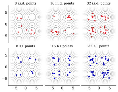
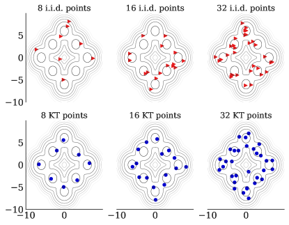
Figure 2: Kernel thinning (KT) and i.i.d. coresets for 4- and 8-component mixture of Gaussian targets with equidensity contours of the target underlaid. See Sec. 7.2 for more details.

7.2 Kernel thinning versus i.i.d. sampling

We first illustrate the benefits of kernel thinning over i.i.d. sampling from a target $\mathbb{P}$. We generate each input sequence $\mathcal{S}_{n}$ i.i.d. from $\mathbb{P}$, use squared kernel bandwidth $\sigma^{2}=2d$, and consider both Gaussian targets $\mathbb{P}=\mathcal{N}(0,\mathbf{I}_{d})$ for $d\in\mathopen{}\mathclose{{}\left\{2,4,10,100}\right\}$ and mixture of Gaussians (MoG) targets $\mathbb{P}=\frac{1}{M}\sum_{j=1}^{M}\mathcal{N}(\mu_{j},\mathbf{I}_{2})$ with $M\in\mathopen{}\mathclose{{}\left\{4,6,8}\right\}$ component locations $\mu_{j}\in\mathbb{R}^{2}$ defined in Sec. P.1.

Fig. 2 highlights the visible differences between the KT and i.i.d. coresets for the MoG targets. Even for small sample sizes, the KT coresets achieves better stratification across components with less clumping and fewer gaps within components, suggestive of a better approximation to $\mathbb{P}$. Indeed, when we examine MMD error as a function of coreset size in Fig. 3(a), we observe that kernel thinning provides a significant improvement across all settings. For the Gaussian $d=2$ target and each MoG target, the KT MMD error scales as $n^{-\frac{1}{2}}$, a quadratic improvement over the $\Omega_{p}(n^{-\frac{1}{4}})$ MMD error of i.i.d. sampling. As we detail in Sec. P.2, we would not expect to see an exact empirical rate of $n^{-\frac{1}{2}}$ for larger $d$ and small $n$ due to the logarithmic factors in our MMD bounds. However, even for small sample sizes and high dimensions, we observe in Fig. 3(b) that KT significantly improves both the magnitude and the decay rate of MMD relative to i.i.d. sampling.

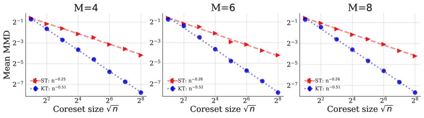
(a) Mixture of Gaussians $\mathbb{P}$

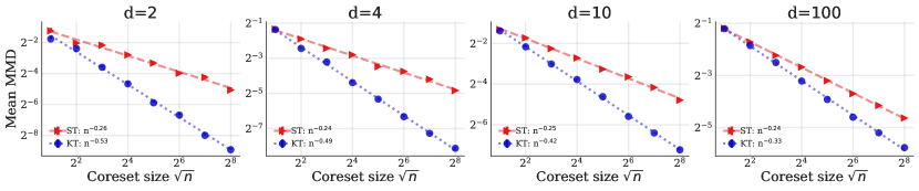
(b) Gaussian $\mathbb{P}$

Figure 3: Kernel thinning versus i.i.d. sampling. For (a) mixture of Gaussian targets with $M\in\mathopen{}\mathclose{{}\left\{4,6,8}\right\}$ components and (b) standard multivariate Gaussian targets in dimension $d\in\mathopen{}\mathclose{{}\left\{2,4,10,100}\right\}$, kernel thinning (KT) reduces $\operatorname{MMD}_{{\mathbf{k}_{\star}}}(\mathbb{P},\mathcal{S})$ significantly more quickly than the standard $n^{-\frac{1}{4}}$ rate for $n^{\frac{1}{2}}$ i.i.d. points, even in high dimensions.

 

7.3 Kernel thinning versus standard MCMC thinning

Next, we illustrate the benefits of kernel thinning over standard Markov chain Monte Carlo (MCMC) thinning on twelve posterior inference experiments conducted by Riabiz et al. [72]. We briefly describe each experiment here and refer the reader to Riabiz et al. [72, Sec. 4] for more details.

Goodwin and Lotka-Volterra experiments

From Riabiz et al. [71], we obtain the output of four distinct MCMC procedures targeting each of two $d=4$-dimensional posterior distributions $\mathbb{P}$: (1) a posterior over the parameters of the Goodwin model of oscillatory enzymatic control [31] and (2) a posterior over the parameters of the Lotka-Volterra model of oscillatory predator-prey evolution [55, 89]. For each target, Riabiz et al. [71] provide $2\times 10^{6}$ sample points from each of four MCMC algorithms: Gaussian random walk (RW), adaptive Gaussian random walk [adaRW, 35], Metropolis-adjusted Langevin algorithm [MALA, 74], and pre-conditioned MALA [pMALA, 30].

Hinch experiments

From Riabiz et al. [71], we also obtain the output of two independent Gaussian random walk MCMC chains for each of two $d=38$-dimensional posterior distributions $\mathbb{P}$: (1) a posterior over the parameters of the Hinch model of calcium signalling in cardiac cells [39] and (2) a tempered version of the same posterior, as defined by Riabiz et al. [72, App. S5.4]. In computational cardiology, the calcium signalling model represents one component of a heart simulator, and one aims to propagate uncertainty in the signalling model through the whole heart simulation, an operation which requires 1000s of CPU hours per sample point [72]. In this setting, the costs of running kernel thinning are dwarfed by the time required to generate the input sample (two weeks) and more than offset by the cost savings in the downstream uncertainty propagation task.

Preprocessing and kernel settings

We discard the initial points of each chain as burn-in using the maximum burn-in period reported in Riabiz et al. [72, Tabs. S4 & S6, App. S5.4]. and normalize each Hinch chain by subtracting the post-burn-in sample mean and dividing each coordinate by its post-burn-in sample standard deviation. To form an input sequence $\mathcal{S}_{n}$ of length $n$ for coreset construction, we downsample the remaining points using standard thinning. Since exact computation of $\operatorname{MMD}_{\mathbf{k}_{\star}}(\mathbb{P},\mathcal{S})$ is intractable for these posterior targets, we report $\operatorname{MMD}_{\mathbf{k}_{\star}}(\mathcal{S}_{n},\mathcal{S})$—the error that is controlled directly in our theoretical results—for these experiments. We select the kernel bandwidth $\sigma$ using the popular median heuristic [see, e.g., 29]. Additional details can be found in Sec. P.3.

   

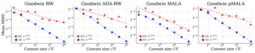
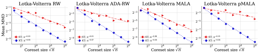
Figure 4: Kernel thinning versus standard MCMC thinning. Kernel thinning (KT) significantly improves both the rate of decay and the order of magnitude of mean $\operatorname{MMD}_{{\mathbf{k}_{\star}}}(\mathcal{S}_{n},\mathcal{S})$ in each posterior inference task, including eight tasks with 4-dimensional targets (Goodwin and Lotka-Volterra) and four tasks with 38-dimensional targets (Hinch). See Sec. 7.3 for more details.

Results

Fig. 4 compares the mean $\operatorname{MMD}_{\mathbf{k}_{\star}}(\mathcal{S}_{n},\mathcal{S})$ error of the generated kernel thinning and standard thinning coresets. In each of the twelve experiments, KT significantly improves both the rate of decay and the order of magnitude of mean MMD, in line with the guarantees of Thm. 1. Notably, in the $d=38$-dimensional Hinch experiments, standard thinning already improves upon the $n^{-\frac{1}{4}}$ rate of i.i.d. subsampling but is outpaced by KT which consistently provides further improvements.

8 Discussion

We introduced kernel thinning (Alg. 1), a new, practical solution to the thinned MMD coreset problem that, given $\mathcal{O}(n^{2})$ time and $\mathcal{O}(n\min(d,n))$ storage, improves upon the integration error of i.i.d. sampling and standard MCMC thinning. To achieve this we first showed that any $L^{\infty}$ coreset for a square-root kernel ${\mathbf{k}}_{\mathrm{rt}}$ also provides an MMD coreset for its associated target kernel ${\mathbf{k}_{\star}}$ (Thm. 2). We next introduced and analyzed a self-balancing Hilbert walk for solving the online vector balancing problem in Hilbert spaces (Algs. 5 and 3). We then designed a symmetrized version of SBHW for RKHSes—kernel halving—that delivers $2$-thinned coresets with small $L^{\infty}$ error (Algs. 3 and 4). Our online algorithm, [algo:ktsplit]kt-split, recursively applies kernel halving to a square-root kernel to obtain near-optimal $L^{\infty}$ coresets in $\mathcal{O}(n^{2})$ time with $\mathcal{O}(n\min(d,n))$ space (Cors. 3 and 5). Kernel thinning then combines [algo:ktsplit]kt-split with a greedy refinement step ([algo:ktswap]kt-swap) to yield coresets with better-than-i.i.d. MMD for a broad range of kernels and target distributions (Thms. 1 and 1). While our analysis is restricted to kernels that admit square-root dominating kernels, [25] recently generalized the KT algorithm and analysis to support arbitrary kernels. Separately, [78] have developed a distribution compression meta-algorithm, Compress++, which reduces the runtime of KT to near-linear $\mathcal{O}(n\log^{3}n)$ time with MMD error that is worse by at most a factor of $4$. Hence, KT-Compress++ can be practically deployed even for very large input sizes.

8.1 Related work on MMD coresets

While $(n^{\frac{1}{2}},o_{p}(n^{-\frac{1}{4}}))$-MMD coresets have been developed for specific $(\mathbb{P},{\mathbf{k}_{\star}})$ pairings like the uniform distribution on the unit cube paired with a Sobolev kernel ${\mathbf{k}_{\star}}$, to the best of our knowledge, no prior $(n^{\frac{1}{2}},o_{p}(n^{-\frac{1}{4}}))$-MMD coreset constructions were known for the range of $\mathbb{P}$ and ${\mathbf{k}_{\star}}$ studied in this work. For comparison, we review here both lower bounds and prior strategies for generating coresets with small MMD.

Lower bounds

For any bounded and radial (i.e., ${\mathbf{k}_{\star}}(x,y)\!=\!\kappa(\mathopen{}\mathclose{{}\left\|{x\!-\!y}}\right\|_{2}^{2})$) kernel satisfying mild decay and smoothness conditions, Phillips and Tai [69, Thm. 3.1] showed that any procedure outputting coresets of size $n^{\frac{1}{2}}$ must suffer $\Omega(\min(\sqrt{d}n^{-\frac{1}{2}},n^{-\frac{1}{4}}))$ $\operatorname{MMD}_{{\mathbf{k}_{\star}}}$ for some (discrete) target distribution $\mathbb{P}$. This lower bound applies, for example, to Matérn kernels and to infinitely smooth Gaussian kernels. For any continuous and shift-invariant (i.e., ${\mathbf{k}_{\star}}(x,y)\!=\!\kappa(x\!-\!y)$) kernel taking on at least two values, Tolstikhin et al. [86, Thm. 1] showed that any estimator (including non-coreset estimators) based only on $n$ i.i.d. draws from $\mathbb{P}$ must suffer $C_{{\mathbf{k}_{\star}}}n^{-\frac{1}{2}}$ $\operatorname{MMD}_{{\mathbf{k}_{\star}}}$ with probability at least $1/4$ for some discrete target $\mathbb{P}$ and a constant $C_{{\mathbf{k}_{\star}}}$ depending only ${\mathbf{k}_{\star}}$. If, in addition, ${\mathbf{k}_{\star}}$ is characteristic (i.e., $\operatorname{MMD}_{\mathbf{k}_{\star}}(\mu,\nu)\neq 0$ when $\mu\!\neq\!\nu$), then Tolstikhin et al. [86, Thm. 6] establish the same lower bound for some continuous target $\mathbb{P}$ with infinitely differentiable density. These last two lower bounds hold, for example, for Gaussian, Matérn, and B-spline kernels and apply in particular to any thinning algorithm that compresses $n$ i.i.d. sample points without additional knowledge of $\mathbb{P}$. For light-tailed $\mathbb{P}$ and ${\mathbf{k}}_{\mathrm{rt}}$, the kernel thinning guarantees of Thm. 1 match each of these lower bounds up to factors of $\sqrt{\log n}$ and constants depending on $d$.

Order $(n^{\frac{1}{2}},n^{-\frac{1}{4}})$-MMD coresets for general target $\mathbb{P}$

By Prop. A.1 of Tolstikhin et al. [86], an i.i.d. sample from $\mathbb{P}$ yields an order $(n^{\frac{1}{2}},n^{-\frac{1}{4}})$-MMD coreset in probability. Chen et al. [20] showed that kernel herding with a finite-dimensional kernel (like the linear ${\mathbf{k}_{\star}}(x,y)=\langle{x},{y}\rangle$) finds an $(n^{\frac{1}{2}},(C_{\mathbb{P},{\mathbf{k}_{\star}},d}n)^{-\frac{1}{2}})$-MMD coreset for an inexplicit parameter $C_{\mathbb{P},{\mathbf{k}_{\star}},d}$. However, Bach et al. [3] showed that their analysis does not apply to any infinite-dimensional kernel (like the Gaussian, Matérn, and B-spline kernels studied in this work), as $C_{\mathbb{P},{\mathbf{k}_{\star}},d}$ would necessarily equal $0$. The best known rate for kernel herding with bounded infinite-dimensional kernels [52, Thm. G.1] guarantees an order $(n^{\frac{1}{2}},n^{-\frac{1}{4}})$-MMD coreset, matching the i.i.d. guarantee. For bounded kernels, the same guarantee is available for Stein Point MCMC [19, Thm. 1] which greedily minimizes MMD over random draws from $\mathbb{P}$ and for a variant of the greedy sign selection algorithm described in Karnin and Liberty [46, Sec. 3.1]. Slightly inferior guarantees were established for Stein points [18, Thm. 1] and Stein thinning [72, Thm. 1], both of which accommodate unbounded kernels as well.

Finite-dimensional kernels

Harvey and Samadi [36] construct $(n^{\frac{1}{2}},\sqrt{d}n^{-\frac{1}{2}}\log^{2.5}n)$-MMD coresets for finite-dimensional linear kernels on $\mathbb{R}^{d}$ but do not address infinite-dimensional kernels.

Uniform distribution on $[0,1]^{d}$

The explicit low discrepancy quasi-Monte Carlo (QMC) construction of Chen and Skriganov [17] provides a $(n^{\frac{1}{2}},\mathcal{O}_{d}(n^{-\frac{1}{2}}\log^{\frac{d-1}{2}}n))$-MMD coreset for an $L^{2}$ discrepancy kernel when $\mathbb{P}$ is the uniform distribution on the unit cube $[0,1]^{d}$. For the same target, the online Haar strategy of Dwivedi et al. [26] yields an $(n^{\frac{1}{2}},\mathcal{O}_{d}(n^{-\frac{1}{2}}\log^{2d}n))$-MMD coreset in probability. Dwivedi et al. [26] also conjecture that a greedy variant of their Haar strategy would provide an improved $(n^{\frac{1}{2}},\mathcal{O}_{d}(n^{-\frac{1}{2}}\log^{d}n))$-MMD coreset. These constructions satisfy our quality criteria but are tailored specifically to the uniform distribution on the unit cube.

Unknown coreset quality

On compact manifolds, optimal coresets of size $n^{\frac{1}{2}}$ minimize the weighted Riesz energy (a form of relative MMD with a weighted Riesz kernel) at known rates [11]; however, practical minimum Riesz energy [11] and minimum energy design [43, 44] constructions have not been analyzed. When ${\mathbf{k}_{\star}}$ is nonnegative and the kernel matrix $({\mathbf{k}_{\star}}(x_{i},x_{j}))_{i,j=1}^{n}$ satisfies a strong diagonal dominance condition, Kim et al. [50, Cor. 3, Thm. 6] show that greedy optimization of $\operatorname{MMD}_{{\mathbf{k}_{\star}}}$ yields an MMD-critic coreset $\hat{\mathcal{S}}$ of size $n^{\frac{1}{2}}$ satisfying

$$\textstyle\operatorname{MMD}_{{\mathbf{k}_{\star}}}^{2}(\mathbb{P}_{n},\hat{\mathcal{S}})\leq(1-\frac{1}{e})\operatorname{MMD}_{\star}^{2}+\frac{1}{e}\mathbb{P}_{n}\mathbb{P}_{n}{\mathbf{k}_{\star}}\quad\text{for}\quad\operatorname{MMD}_{\star}=\min_{|\mathcal{S}|=\sqrt{n}}\operatorname{MMD}_{{\mathbf{k}_{\star}}}(\mathbb{P}_{n},\mathcal{S}).$$ (24)

In the usual case when $\mathbb{P}_{n}\mathbb{P}_{n}{\mathbf{k}_{\star}}=\Omega(1)$, this error bound does not decay to $0$ with $n$. Paige et al. [66] analyze the impact of approximating a kernel in super-sampling with a reservoir but do not analyze the quality of the constructed MMD coreset. For the conditionally positive definite energy distance kernel, Mak and Joseph [56] establish that an optimal coreset of size $n^{\frac{1}{2}}$ has $o(n^{-\frac{1}{4}})$ MMD but do not provide a construction; in addition, Mak and Joseph [56] propose two support points convex-concave procedures for constructing MMD coresets but do not establish their optimality and do not analyze their quality.

8.2 Related work on weighted MMD coresets

While coresets satisfy a number of valuable constraints that are critical for some downstream applications—exact approximation of constants, automatic preservation of convex integrand constraints, compatibility with unweighted downstream tasks, easy visualization, straightforward sampling, and increased numerical stability against errors in integral evaluations [48]—some applications also support weighted coreset approximations of $\mathbb{P}$ of the form $\sum_{i=1}^{\sqrt{n}}w_{i}\boldsymbol{\delta}_{x_{i}}$ for weights $w_{i}\in\mathbb{R}$ that need not be equal, need not be nonnegative, or need not sum to $1$. Notably, weighted coresets that depend on $\mathbb{P}$ only through an i.i.d. sample of size $n$ are subject to the same $\Omega(n^{-\frac{1}{2}})$ MMD lower bounds of Tolstikhin et al. [86] described in Sec. 8.1. Any constructions that violate these bounds do so only by exploiting additional information about $\mathbb{P}$ (for example, exact knowledge of $\mathbb{P}{\mathbf{k}_{\star}}$) that is not generally available and not required for our kernel thinning guarantees. Moreover, while weighted coresets need not provide satisfactory solutions to the unweighted coreset problem studied in this work, kernel thinning coreset points can be converted into an optimally weighted coreset of no worse quality by explicitly minimizing $\operatorname{MMD}_{{\mathbf{k}_{\star}}}(\mathbb{P}_{n},\sum_{i=1}^{\sqrt{n}}w_{i}\boldsymbol{\delta}_{x_{i}})$ or, if computable, $\operatorname{MMD}_{{\mathbf{k}_{\star}}}(\mathbb{P},\sum_{i=1}^{\sqrt{n}}w_{i}\boldsymbol{\delta}_{x_{i}})$ over the weights $w_{i}$ in $\mathcal{O}(n^{3/2})$ time.

With this context, we now review known weighted MMD coreset guarantees. We highlight that only one of the weighted $(n^{\frac{1}{2}},o(n^{-\frac{1}{4}}))$-MMD guarantees covers the unbounded distributions addressed in this work and that the single unbounded guarantee relies on a restrictive uniformly bounded eigenfunction assumption that is typically not satisfied. In other words, our analysis establishes MMD improvements for practical $({\mathbf{k}_{\star}},\mathbb{P})$ pairings not covered by prior weighted analyses.

$\mathbb{P}$ with bounded support

If the target $\mathbb{P}$ has bounded density and bounded, regular support and ${\mathbf{k}_{\star}}$ is a Gaussian or Matérn kernel, then Bayesian quadrature [64] and Bayes-Sard cubature [47] with quasi-uniform unisolvent point sets yield weighted $(n^{\frac{1}{2}},o(n^{-\frac{1}{4}}))$-MMD coresets by Wendland [91, Thm. 11.22 and Cor. 11.33]. If $\mathbb{P}$ has bounded support, and ${\mathbf{k}_{\star}}$ has more than $d$ continuous derivatives, then the P-greedy algorithm [21] also yields weighted $(n^{\frac{1}{2}},o(n^{-\frac{1}{4}}))$-MMD coresets by Santin and Haasdonk [76, Thm. 4.1]. For $({\mathbf{k}_{\star}},\mathbb{P})$ pairs with compact support and sufficiently rapid eigenvalue decay, approximate continuous volume sampling kernel quadrature [9] using the Gibbs sampler of Rezaei and Gharan [70] yields weighted coresets with $o(n^{-\frac{1}{4}})$ root mean squared MMD.

Finite-dimensional kernels with compactly supported $\mathbb{P}$

For compactly supported $\mathbb{P}$, Briol et al. [13, Thm. 1] and Bach et al. [3, Prop. 1] show that Frank-Wolfe Bayesian quadrature and weighted variants of kernel herding respectively yield weighted $(n^{\frac{1}{2}},o(n^{-\frac{1}{4}}))$-MMD coresets for continuous finite-dimensional kernels, but, by Bach et al. [3, Prop. 2], these analyses do not extend to infinite-dimensional kernels, like the Gaussian, Matérn, and B-spline kernels studied in this work.

Eigenfunction restrictions

For $({\mathbf{k}_{\star}},\mathbb{P})$ pairs with known Mercer eigenfunctions, Belhadji et al. [8] bound the expected squared MMD of determinantal point process (DPP) kernel quadrature in terms of kernel eigenvalue decay and provide explicit rates for univariate Gaussian $\mathbb{P}$ and uniform $\mathbb{P}$ on $[0,1]$. Their construction makes explicit use of the kernel eigenfunctions which are not available for most $({\mathbf{k}_{\star}},\mathbb{P})$ pairings. For $({\mathbf{k}_{\star}},\mathbb{P})$ pairs with $\mathbb{P}{\mathbf{k}_{\star}}={\boldsymbol{0}}$, uniformly bounded eigenfunctions, and rapidly decaying eigenvalues, Liu and Lee [54, App. B.2] prove that black-box importance sampling generates probability-weighted coresets with $o(n^{-\frac{1}{4}})$ root mean squared MMD but do not provide any examples verifying their assumptions. The uniformly bounded eigenfunction condition is considered particularly difficult to check [82], does not hold for Gaussian kernels with Gaussian $\mathbb{P}$ [58, Thm. 1], and need not hold even for infinitely univariate smooth kernels on $[0,1]$ [93, Ex. 1].

Unknown coreset quality

Huszár and Duvenaud [42, Prop. 2] bound the MMD error of weighted sequential Bayesian quadrature coresets using weak submodularity, but this bound does not decay to zero with $n$. Khanna and Mahoney [49, Thm. 2] prove that weighted kernel herding yields a weighted $(n^{\frac{1}{2}},\exp(-n^{\frac{1}{2}}/\kappa_{n}))$-MMD coreset. However, the $\kappa_{n}$ term in Khanna and Mahoney [49, Thm.3, Assum. 2] is at least as large as the condition number of an $\sqrt{n}\times\sqrt{n}$ kernel matrix, which for typical kernels (including the Gaussian and Matérn kernels) is $\Omega(\sqrt{n})$ [51, 27]; the resulting MMD error bound therefore does not decay with $n$. The ProtoGreedy and ProtoDash algorithms of Gurumoorthy et al. [34, Thm. IV.3, IV.5] yield nonnegative weighted coresets $\hat{\mathcal{S}}$ of size $n^{\frac{1}{2}}$ satisfying $\operatorname{MMD}_{{\mathbf{k}_{\star}}}^{2}(\mathbb{P}_{n},\hat{\mathcal{S}})\leq\operatorname{MMD}_{\star}^{2}+(\mathbb{P}_{n}\mathbb{P}_{n}{\mathbf{k}_{\star}}-\operatorname{MMD}_{\star}^{2})e^{-\lambda_{\sqrt{n}}}$ where $\operatorname{MMD}_{\star}$ is the optimal MMD error to $\mathbb{P}_{n}$ for a nonnegatively weighted coreset of size $n^{\frac{1}{2}}$. However, careful inspection reveals that $\lambda_{\sqrt{n}}\leq 1$ for any kernel and any $n$. Hence, in the usual case in which $\mathbb{P}_{n}\mathbb{P}_{n}{\mathbf{k}_{\star}}=\Omega(1)$, this error bound does not decay to $0$ with $n$. Campbell and Broderick [16, Thm. 4.4] prove that Hilbert coresets via Frank-Wolfe with $n$ input points yield weighted order $(n^{\frac{1}{2}},\nu_{n}^{\sqrt{n}})$-MMD coresets for some $\nu_{n}<1$ but do not analyze the dependence of $\nu_{n}$ on $n$.

Non-MMD guarantees

For $\mathbb{P}$ with continuously differentiable Lebesgue density and ${\mathbf{k}_{\star}}$ a bounded Langevin Stein kernel with $\mathbb{P}{\mathbf{k}_{\star}}={\boldsymbol{0}}$, Thm. 2 of Oates et al. [62] does not bound MMD but does prove that a randomized control functionals weighted coreset satisfies $\sqrt{\mathbb{E}[(\mathbb{E}f-\sum_{i=1}^{\sqrt{n}}w_{i}f(x_{i}))^{2}]}\leq{C_{\mathbb{P},{\mathbf{k}_{\star}},d,f}}{/n^{\frac{7}{24}}}$ for each $f$ in the RKHS of ${\mathbf{k}_{\star}}$ and an unspecified $C_{\mathbb{P},{\mathbf{k}_{\star}},d,f}$. This bound is asymptotically better than the $\Omega(n^{-\frac{1}{4}})$ guarantee for unweighted i.i.d. coresets but worse than the unweighted kernel thinning guarantees of Thm. 1. On compact domains, Thm. 1 of Oates et al. [63] establishes improved rates for the same weighted coreset when both $\mathbb{P}$ and ${\mathbf{k}_{\star}}$ are sufficiently smooth. Bardenet and Hardy [5] establish an $n^{-\frac{1}{4}-\frac{1}{4d}}$ asymptotic decay of $\mathbb{E}f-\sum_{i=1}^{\sqrt{n}}w_{i}f(x_{i})$ for DPP kernel quadrature with $\mathbb{P}$ on $[-1,1]^{d}$ and each $f$ in the RKHS of a particular kernel.

8.3 Related work on $L^{\infty}$ coresets

A number of alternative strategies are available for constructing coresets with $L^{\infty}$ guarantees. For example, for any bounded ${\mathbf{k}}_{\mathrm{rt}}$, Cauchy-Schwarz and the reproducing property imply that

$$\textstyle\mathopen{}\mathclose{{}\left\|{(\mathbb{P}-\mathbb{P}_{n}){\mathbf{k}_{\star}}}}\right\|_{\infty}=\sup_{z\in\mathbb{R}^{d}}\mathopen{}\mathclose{{}\left|\mathopen{}\mathclose{{}\left\langle{\mathbf{k}_{\star}}(z,\cdot),\mathbb{P}{\mathbf{k}_{\star}}-\mathbb{P}_{n}{\mathbf{k}_{\star}}}\right\rangle_{{\mathbf{k}_{\star}}}}\right|\leq\operatorname{MMD}_{{\mathbf{k}_{\star}}}(\mathbb{P},\mathbb{P}_{n})\cdot\mathopen{}\mathclose{{}\left\|{{\mathbf{k}_{\star}}}}\right\|_{\infty}^{\frac{1}{2}},$$ (25)

so that all of the order $(n^{\frac{1}{2}},n^{-\frac{1}{4}})$-MMD coreset constructions discussed in Sec. 8.1 also yield order $(n^{\frac{1}{2}},n^{-\frac{1}{4}})$-$L^{\infty}$ coresets. However, none of those constructions is known to provide a $(n^{\frac{1}{2}},o(n^{-\frac{1}{4}}))$-$L^{\infty}$ coreset.

A series of breakthroughs due to Joshi et al. [45], Phillips [67], Phillips and Tai [68, 69], Tai [85] has led to a sequence of increasingly compressed $(n^{\frac{1}{2}},o(n^{-\frac{1}{4}}))$-$L^{\infty}$ coreset constructions, with the best known guarantees currently due to Phillips and Tai [69] and Tai [85]. Given $n$ input points, Phillips and Tai [69] developed an offline, polynomial-time construction to find an $(n^{\frac{1}{2}},\mathcal{O}_{p}(\sqrt{d}n^{-\frac{1}{2}}\sqrt{\log n}))$-$L^{\infty}$ coreset for Lipschitz kernels exhibiting suitable decay, while Tai [85] developed an offline construction for Gaussian kernels that runs in $\Omega(d^{5d})$ time and yields an $(n^{\frac{1}{2}},\mathcal{O}_{p}(2^{d}n^{-\frac{1}{2}}\sqrt{\log(d\log n)}))$-$L^{\infty}$ coreset. More details on these constructions based on the Gram-Schmidt walk of Bansal et al. [4] can be found in App. S. Notably, the Phillips and Tai (hereafter, PT) guarantee is tighter than that of Thm. 4 by a factor of $\sqrt{\log\log n}$ for sub-Gaussian kernels and input points and $\sqrt{\log n}$ for heavy-tailed kernels and input points. Similarly, the Tai guarantee provides an improvement when $n$ is doubly-exponential in the dimension, that is, when $\sqrt{d\log n}=\Omega(2^{d})$.

Moreover, by Thm. 2, we may apply the PT and Tai constructions to a square-root kernel ${\mathbf{k}}_{\mathrm{rt}}$ to obtain comparable MMD guarantees for the target kernel ${\mathbf{k}_{\star}}$ with high probability. However, kernel thinning has a number of practical advantages that lead us to recommend it. First with $n$ input points, using standard matrix multiplication, the PT and Tai constructions have $\Omega(n^{4})$ computational complexity and $\Omega(n^{2})$ storage costs, a substantial increase over the $\mathcal{O}(n^{2})$ running time and $\mathcal{O}(n\min(d,n))$ storage of kernel thinning. Second, [algo:ktsplit]kt-split is an online algorithm while the PT and Tai constructions require the entire set of input points to be available a priori. Finally, each halving round of [algo:ktsplit]kt-split splits the sample size exactly in half, allowing the user to run all $m$ halving rounds simultaneously; the PT and Tai constructions require a rebalancing step after each round forcing the halving rounds to be conducted sequentially.

8.4 Future directions

Several other opportunities for future development recommend themselves. First, since our results cover any target $\mathbb{P}$ with at least $2d$ moments—even discrete and other non-smooth targets—a natural question is whether tighter error bounds with better sample complexities are available when $\mathbb{P}$ is also known to have a smooth Lebesgue density. Second, the MMD to $L^{\infty}$ reduction in Thm. 2 applies also to weighted $L^{\infty}$ coresets, and, in applications in which weighted point sets are supported, we would expect either quality or compression improvements from employing non-uniform weights [see, e.g. 87].

Appendix

Contents

1. 1 Introduction
   1. 1.1 Thinned MMD coresets
   2. 1.2 Our contributions
2. 2 Input Point and Kernel Requirements
   1. 2.1 Input point requirements
   2. 2.2 Kernel requirements
3. 3 Kernel Thinning
4. 4 MMD Guarantees
   1. 4.1 MMD guarantees for kernel thinning
   2. 4.2 MMD coresets from square-root $L^{\infty}$ coresets
5. 5 Self-balancing Hilbert Walk
6. 6 $L^{\infty}$ Guarantees
   1. 6.1 $L^{\infty}$ guarantees for kernel halving
   2. 6.2 $L^{\infty}$ and MMD guarantees for KT-SPLIT
7. 7 Vignettes
   1. 7.1 Common settings
   2. 7.2 Kernel thinning versus i.i.d. sampling
   3. 7.3 Kernel thinning versus standard MCMC thinning
8. 8 Discussion
   1. 8.1 Related work on MMD coresets
   2. 8.2 Related work on weighted MMD coresets
   3. 8.3 Related work on $L^{\infty}$ coresets
   4. 8.4 Future directions
9. A Appendix Notation
10. B Proof of Prop. 1: MMD guarantee for MCMC
11. C Proof of Prop. 2: *prop:radii_growth
    1. C.1 Radius growth for identically distributed sequences
       1. C.1.1 Proof of Lem. 1: *lemma:identical_growth_rate
    2. C.2 Radius growth for MCMC
       1. C.2.1 Proof of Lem. 5: *lemma:mcmc_growth_rate
12. D Proof of Prop. 3: Shift-invariant square-root kernels
13. E Proof of Thm. 1: MMD guarantee for kernel thinning
14. F Proof of Rem. 4: Finite-time and anytime guarantees
15. G Proof of Cor. 1: MMD rates for kernel thinning
16. H Proof of Thm. 2: MMD guarantee for square-root $L^{\infty}$ approximations
    1. H.1 Proof of Lem. 7: Square-root representation of MMD
    2. H.2 Proof of Lem. 8: $L^{\infty}$ bound on ${L}^{2}$ kernel error
17. I Proof of Cor. 2: MMD error from square-root $L^{\infty}$ error
18. J Proof of Thm. 3: Self-balancing Hilbert walk properties
    1. J.1 Property (i): Functional sub-Gaussianity
    2. J.2 Property (ii): Signed sum representation
    3. J.3 Property (iii): Exact halving via symmetrization
    4. J.4 Property (iv): Pointwise sub-Gaussianity in RKHS
    5. J.5 Property (v): Sub-Gaussian constant bound
    6. J.6 Property (vi): Adaptive thresholding
    7. J.7 Proof of Lem. 9: Alternate representation of $\psi_{i}$
19. K Proof of Thm. 4: $L^{\infty}$ guarantees for kernel halving
    1. K.1 Proof of part (a): Kernel halving yields a $2$-thinned $L^{\infty}$ coreset
       1. K.1.1 Proof for case (I): When $R_{\mathcal{S}_{n},\mathbf{k},n}<R_{\mathcal{S}_{n}}$
       2. K.1.2 Proof for case (II): When $R_{\mathcal{S}_{n},\mathbf{k},n}=R_{\mathcal{S}_{n}}$
    2. K.2 Proof of part (b): Repeated kernel halving yields a $2^{m}$-thinned $L^{\infty}$ coreset
       1. K.2.1 Proof for case (I): When $R_{\mathcal{S}_{n},\mathbf{k},n}<R_{\mathcal{S}_{n}}$
       2. K.2.2 Proof for case (II): When $R_{\mathcal{S}_{n},\mathbf{k},n}=R_{\mathcal{S}_{n}}$
    3. K.3 Proof of Lem. 11: A direct covering bound on $\|\psi_{n/2}\|_{\infty}$
       1. K.3.1 Proof of 207
       2. K.3.2 Proof of 208
    4. K.4 Proof of Lem. 12: A basic bound on $\|\psi_{n/2}\|_{\infty}$
    5. K.5 Proof of Lem. 13: A high probability bound on supremum of $\psi_{n/2}$ differences
    6. K.6 Proof of Lem. 18: $\psi_{n/2}$ is an Orlicz $\Psi_{2}$-process
    7. K.7 Proof of Lem. 19: Bounds on $\mathcal{N}_{\mathbb{T},\rho}$ and $\mathcal{J}_{\mathbb{T},\rho}$
20. L Proof of Rem. 8: Example settings for KH $L^{\infty}$ rates
21. M Proof of Cor. 5: $L^{\infty}$ and MMD guarantees for [algo:ktsplit]kt-split
22. N Derivation of Tab. 2: Square-root kernels ${\mathbf{k}}_{\mathrm{rt}}$ for common target kernels ${\mathbf{k}_{\star}}$
    1. N.1 General proof strategy
    2. N.2 Deriving ${\mathbf{k}}_{\mathrm{rt}}$ for the Matérn kernel
    3. N.3 Deriving ${\mathbf{k}}_{\mathrm{rt}}$ for the B-Spline kernel
23. O Derivation of Tab. 4: Explicit bounds on Thm. 1 quantities for common kernels
    1. O.1 Common tools for our derivations
    2. O.2 Proofs for Gaussian kernel
    3. O.3 Proofs for Matérn kernel
       1. O.3.1 Set-up for proofs of Matérn kernel quantities
       2. O.3.2 Proof of the bound 289 on $\mathopen{}\mathclose{{}\left\|{{\mathbf{k}}_{\mathrm{rt}}}}\right\|_{\infty}$ and $\mathopen{}\mathclose{{}\left\|{{\mathbf{k}_{\star}}}}\right\|_{\infty}$
       3. O.3.3 Proof of the bound 290 on $A_{\nu,\gamma,d}$
       4. O.3.4 Proof of the bound 291 on $L_{{\mathbf{k}}_{\mathrm{rt}}}$
       5. O.3.5 Proof of the bound 292 on $R_{{\mathbf{k}}_{\mathrm{rt}},n}$
       6. O.3.6 Proof of the bound 293 on $R_{{\mathbf{k}}_{\mathrm{rt}},\sqrt{n}}^{\prime}$
    4. O.4 Proofs for B-spline kernel
       1. O.4.1 Proofs of the bounds on B-spline kernel quantities
    5. O.5 Explicit MMD rates for common kernels
24. P Supplementary Details for Vignettes of Sec. 7
    1. P.1 Mixture of Gaussians target
    2. P.2 Empirical decay rates
    3. P.3 MCMC vignette details
25. Q Kernel Thinning with Square-root Dominating Kernels
    1. Q.1 Proof of Prop. 4: Dominating smooth kernels
    2. Q.2 Proof of Prop. 5: Dominating shift-invariant kernels
    3. Q.3 Derivation of Tab. 10: Square-root dominating kernels $\widetilde{\mathbf{k}}_{\mathrm{rt}}$ for common kernels ${\mathbf{k}_{\star}}$
26. R Online Vector Balancing in Euclidean Space
27. S $L^{\infty}$ Coresets of Phillips and Tai [69] and Tai [85]

Appendix A Appendix Notation

For each $p\geq 1$, we define ${L}^{p}$ as the set of measurable $g:\mathbb{R}^{d}\to\mathbb{R}$ with $\mathopen{}\mathclose{{}\left\|{g}}\right\|_{L^{p}}\triangleq(\int|g(x)^{p}|dx)^{1/p}<\infty$ and $C^{p}$ as the set of $g:\mathbb{R}^{d}\to\mathbb{R}$ for which all partial derivatives of order $p$ exist and are continuous. For a kernel $\mathbf{k}:\mathbb{R}^{d}\times\mathbb{R}^{d}\to\mathbb{R}$, we also write $\mathbf{k}\in{L}^{2,\infty}$ to indicate that $\mathbf{k}$ is measurable with finite

$$\textstyle\mathopen{}\mathclose{{}\left\|{\mathbf{k}}}\right\|_{L^{2,\infty}}\triangleq\sup_{x\in\mathbb{R}^{d}}\mathopen{}\mathclose{{}\left(\int\mathbf{k}^{2}(x,y)dy}\right)^{\frac{1}{2}}=\sup_{x\in\mathbb{R}^{d}}\mathopen{}\mathclose{{}\left\|{\mathbf{k}(x,\cdot)}}\right\|_{L^{2}}.$$ (26)

Throughout, we follow the unitary angular frequency convention of Wendland [91, Def. 5.15] and define the Fourier transform $\mathcal{F}(f)$ of an integrable complex function $f:\mathbb{R}^{d}\to\mathbb{C}$ via

$$\textstyle\mathcal{F}({f})(\omega)\triangleq\frac{1}{(2\pi)^{{d}/{2}}}\int_{\mathbb{R}^{d}}f(x)e^{-i\langle{x},{\omega}\rangle}dx\quad\text{for all}\quad\omega\in\mathbb{R}^{d}.$$ (27)

Appendix B Proof of Prop. 1: MMD guarantee for MCMC

By Douc et al. [23, Lem. 9.3.9, Cor. 9.2.16], a homogeneous $\phi$-irreducible geometrically ergodic Markov chain with stationary distribution $\mathbb{P}$ is also aperiodic with a unique stationary distribution. Since $(x_{i})_{i=0}^{\infty}$ are the iterates of such a chain, there exist, by Gallegos-Herrada et al. [28, Thm. 1xi], constants $\rho\in(0,1)$ and $\tau<\infty$ and a measurable $\mathbb{P}$-almost everywhere finite function $V:\mathbb{R}^{d}\to[1,\infty]$ satisfying $\mathbb{P}V<\infty$ and

$$\!\sup_{\text{measurable }h:\frac{|h(x)|}{V(x)}\leq 1,\forall x\in\mathbb{R}^{d}}|\mathbb{E}[h(x_{i})\mid x_{0}=x]-\mathbb{P}h|\leq\tau V(x)\rho^{i},\text{ for all }x\in\mathbb{R}^{d}\ \text{and}\ i\in\mathbb{N}.$$ (28)

Since $V$ is finite $\mathbb{P}$-almost everywhere, we will choose $c(x)=\infty\Leftrightarrow V(x)=\infty$ to ensure that our claim is (vacuously) true whenever $V(x_{0})=\infty$.

Hereafter, suppose $V(x_{0})<\infty$. Since the Markov chain is irreducible and aperiodic with a unique stationary distribution $\mathbb{P}$, Assump. H1 of Havet et al. [37] is satisfied. Hence, by an application of Havet et al. [37, Prop. 2.1] with $V^{\prime}=V\rho^{g}$ and $\zeta=2/\rho^{g}$ for sufficiently large $g\in\mathbb{N}$, there exists a set $C(x_{0})\subseteq\mathbb{R}^{d}$ that contains $x_{0}$ and satisfies Assumps. H2 and H3 of Havet et al. [37].

Now fix any $y_{1},\dots,y_{n},z_{1},\dots,z_{n}\in\mathbb{R}^{d}$. We invoke the definition of MMD 1, the triangle inequality, the reproducing property of an RKHS [81, Def. 4.18], and Cauchy-Schwarz in turn to deduce a bounded differences property for MMD:

$$\textstyle\operatorname{MMD}_{{\mathbf{k}_{\star}}}(\mathbb{P},\frac{1}{n}\sum_{i=1}^{n}\boldsymbol{\delta}_{y_{i}})-\operatorname{MMD}_{{\mathbf{k}_{\star}}}(\mathbb{P},\frac{1}{n}\sum_{i=1}^{n}\boldsymbol{\delta}_{z_{i}})$$ (29)

$$\textstyle=\sup_{\|{f}\|_{{\mathbf{k}_{\star}}}\leq 1}|\mathbb{P}f-\frac{1}{n}\sum_{i=1}^{n}f(y_{i})|-\sup_{\|{f}\|_{{\mathbf{k}_{\star}}}\leq 1}|\mathbb{P}f-\frac{1}{n}\sum_{i=1}^{n}f(z_{i})|$$ (30)

$$\textstyle\leq\sup_{\|{f}\|_{{\mathbf{k}_{\star}}}\leq 1}|\frac{1}{n}\sum_{i=1}^{n}f(y_{i})-f(z_{i})|=\sup_{\|{f}\|_{{\mathbf{k}_{\star}}}\leq 1}\frac{1}{n}\sum_{i=1}^{n}|\mathopen{}\mathclose{{}\left\langle{\mathbf{k}_{\star}}(y_{i},\cdot)-{\mathbf{k}_{\star}}(z_{i},\cdot),f}\right\rangle_{{\mathbf{k}_{\star}}}|$$ (31)

$$\textstyle\leq\sup_{\|{f}\|_{{\mathbf{k}_{\star}}}\leq 1}\frac{1}{n}\sum_{i=1}^{n}\|{{\mathbf{k}_{\star}}(y_{i},\cdot)-{\mathbf{k}_{\star}}(z_{i},\cdot)}\|_{{\mathbf{k}_{\star}}}\|{f}\|_{{\mathbf{k}_{\star}}}$$ (32)

$$\textstyle=\sup_{\|{f}\|_{{\mathbf{k}_{\star}}}\leq 1}\frac{1}{n}\sum_{i=1}^{n}\sqrt{{\mathbf{k}_{\star}}(y_{i},y_{i})+{\mathbf{k}_{\star}}(z_{i},z_{i})-2{\mathbf{k}_{\star}}(y_{i},z_{i})}\|{f}\|_{{\mathbf{k}_{\star}}}\leq\frac{2}{n}\mathopen{}\mathclose{{}\left\|{{\mathbf{k}_{\star}}}}\right\|_{\infty}^{\frac{1}{2}}\sum_{i=1}^{n}\mathbb{I}\mathopen{}\mathclose{{}\left[{y_{i}\neq z_{i}}}\right].$$ (33)

Since $x_{0}$ belongs to a set $C(x_{0})$ satisfying Assumps. H2 and H3 of Havet et al. [37], McDiarmid’s inequality for geometrically ergodic Markov chains [37, Thm. 3.1] implies that, with probability at least $1-\delta$ conditional on $x_{0}$,

$$\textstyle\operatorname{MMD}_{{\mathbf{k}_{\star}}}(\mathbb{P},\mathbb{P}_{n})\leq\mathbb{E}[\operatorname{MMD}_{{\mathbf{k}_{\star}}}(\mathbb{P},\mathbb{P}_{n})\mid x_{0}]+\sqrt{c_{1}(x_{0})\mathopen{}\mathclose{{}\left\|{{\mathbf{k}_{\star}}}}\right\|_{\infty}\log(1/\delta)/n}$$ (34)

where $c_{1}(x_{0})$ is a finite value depending only on the transition probabilities of the chain and the set $C(x_{0})$.

Now, define the $\mathbb{P}$ centered kernel ${\mathbf{k}_{\star}}_{\mathbb{P}}(x,y)={\mathbf{k}_{\star}}(x,y)-\mathbb{P}{\mathbf{k}_{\star}}(x)-\mathbb{P}{\mathbf{k}_{\star}}(y)+\mathbb{P}\mathbb{P}{\mathbf{k}_{\star}}$. To bound the expectation, we will use a slight modification of Lem. 3 of Riabiz et al. [72]. The original lemma used the assumption of $V$-uniform ergodicity [57, Defn. (16.0.1)] and the assumption $V(x)\geq\sqrt{{\mathbf{k}_{\star}}_{\mathbb{P}}(x,x)}$ solely to argue that, for some $R>0$,

$$\textstyle|\mathbb{E}[f(x_{i})\mid x_{0}=x]-\mathbb{P}f|\leq RV(x)\rho^{i}\quad\text{for all}\quad x\in\mathbb{R}^{d}\quad\text{and}\quad f\in\mathcal{H}_{{\mathbf{k}_{\star}}_{\mathbb{P}}}\ \text{with}\ \mathopen{}\mathclose{{}\left\|{f}}\right\|_{{\mathbf{k}_{\star}}_{\mathbb{P}}}=1.$$ (35)

In our case, since ${\mathbf{k}_{\star}}_{\mathbb{P}}$ is bounded and any $f\in\mathcal{H}_{{\mathbf{k}_{\star}}_{\mathbb{P}}}$ with $\mathopen{}\mathclose{{}\left\|{f}}\right\|_{{\mathbf{k}_{\star}}_{\mathbb{P}}}=1$ satisfies

$$\textstyle|f(x)|=|\langle{{\mathbf{k}_{\star}}_{\mathbb{P}}(x,\cdot)},{f}\rangle_{{\mathbf{k}_{\star}}_{\mathbb{P}}}|\leq\mathopen{}\mathclose{{}\left\|{{\mathbf{k}_{\star}}_{\mathbb{P}}(x,\cdot)}}\right\|_{{\mathbf{k}_{\star}}_{\mathbb{P}}}\mathopen{}\mathclose{{}\left\|{f}}\right\|_{{\mathbf{k}_{\star}}_{\mathbb{P}}}=\sqrt{{\mathbf{k}_{\star}}_{\mathbb{P}}(x,x)}\leq\sqrt{\mathopen{}\mathclose{{}\left\|{{\mathbf{k}_{\star}}_{\mathbb{P}}}}\right\|_{\infty}}\ \text{for all}\ x\in\mathbb{R}^{d}$$ (36)

by the reproducing property and Cauchy-Schwarz, the geometric ergodicity property 57 implies the analogous bound

$$\textstyle|\mathbb{E}[f(x_{i})\mid x_{0}=x]-\mathbb{P}f|\leq\tau\sqrt{\mathopen{}\mathclose{{}\left\|{{\mathbf{k}_{\star}}_{\mathbb{P}}}}\right\|_{\infty}}V(x)\rho^{i}\ \text{for all}\ x\in\mathbb{R}^{d}\ \text{and}\ f\in\mathcal{H}_{{\mathbf{k}_{\star}}_{\mathbb{P}}}\ \text{with}\ \mathopen{}\mathclose{{}\left\|{f}}\right\|_{{\mathbf{k}_{\star}}_{\mathbb{P}}}=1.$$ (37)

Hence, the conclusions of Riabiz et al. [72, Lem. 3] with $R=\tau\sqrt{\mathopen{}\mathclose{{}\left\|{{\mathbf{k}_{\star}}_{\mathbb{P}}}}\right\|_{\infty}}$ hold under our assumptions. Jensen’s inequality and the conclusion of Lem. 3 of Riabiz et al. [72] now yield the sure bound

$$\textstyle\mathbb{E}[ \textstyle\operatorname{MMD}_{{\mathbf{k}_{\star}}}(\mathbb{P},\mathbb{P}_{n})\mid x_{0}]^{2}\leq\mathbb{E}[\operatorname{MMD}_{{\mathbf{k}_{\star}}}(\mathbb{P},\mathbb{P}_{n})^{2}\mid x_{0}]$$ (38)

$$\textstyle=\mathbb{E}[\frac{1}{n^{2}}\sum_{i=1}^{n}{\mathbf{k}_{\star}}_{\mathbb{P}}(x_{i},x_{i})+\frac{1}{n^{2}}\sum_{i=1}^{n}\sum_{j\neq i}{\mathbf{k}_{\star}}_{\mathbb{P}}(x_{i},x_{j})\mid x_{0}]$$ (39)

$$\textstyle\leq\frac{1}{n}\mathopen{}\mathclose{{}\left\|{{\mathbf{k}_{\star}}_{\mathbb{P}}}}\right\|_{\infty}(1+\frac{2\tau\rho}{1-\rho}\frac{1}{n}\sum_{i=1}^{n-1}\mathbb{E}[V(x_{i})\mid x_{0}])\leq\frac{4}{n}\mathopen{}\mathclose{{}\left\|{{\mathbf{k}_{\star}}}}\right\|_{\infty}(1+\frac{2\tau\rho}{1-\rho}\frac{1}{n}\sum_{i=1}^{n-1}\mathbb{E}[V(x_{i})\mid x_{0}]).$$ (40)

Now, define $c_{2}(x_{0})\triangleq\sup_{n\in\mathbb{N}}\frac{1}{n}\sum_{i=1}^{n-1}\mathbb{E}[V(x_{i})\mid x_{0}]$. Since $V(x_{0})<\infty$, the geometric ergodicity property 57 and the fact that $\mathbb{P}V<\infty$ imply

$$\textstyle c_{2}(x_{0})\leq\mathbb{P}V+V(x_{0})\sup_{n\in\mathbb{N}}{\textstyle\frac{1}{n}}{\textstyle\sum}_{i=1}^{n-1}\rho^{i}\leq\mathbb{P}V+V(x_{0})\rho<\infty.$$ (41)

Taking $c(x_{0})=\sqrt{2}\max(c_{1}(x_{0}),4c_{2}(x_{0})(1+\frac{2\tau\rho}{1-\rho}))$ completes the proof.

Appendix C Proof of Prop. 2: *prop:radii_growth

We prove this result for the identically distributed case in Sec. C.1 and for the Markov chain case in Sec. C.2.

C.1 Radius growth for identically distributed sequences

Suppose $x_{0}$ and $\mathcal{S}_{\infty}$ are drawn identically from $\mathbb{P}$. Claim (a) is true by definition. To establish the remaining claims, we use the following more general result proved in Sec. C.1.1.

Lemma 1 (Growth rate for identically distributed sequence).

Consider a sequence of identically distributed random variables $(Y_{i})_{i=1}^{\infty}$ on $\mathbb{R}$ and a measurable function $\psi:\real\to\real$ with an increasing inverse function $\psi^{-1}$. If $\psi(Y_{1})\geq 0$ almost surely, then

$$\textstyle\mathrm{Pr}(\max_{i\leq n}Y_{i}>\psi^{-1}(n)\ \text{for some}\ n\in\mathbb{N})\leq\mathbb{E}(\psi(Y_{1})).$$ (42)

Consequently, if $\mathbb{E}(\psi(Y_{1}))<\infty$, then, for any $\delta\in(0,1]$,

$$\textstyle\mathrm{Pr}(\max_{i\leq n}Y_{i}\leq\psi^{-1}(\frac{n\mathbb{E}[\psi(\mathopen{}\mathclose{{}\left\|{x_{1}}}\right\|_{2})]}{\delta})\ \text{for all}\ n\in\mathbb{N})\geq 1-\delta.$$ (43)

Fix any $\delta\in(0,1]$. Lem. 1 with $Y_{i}=\mathopen{}\mathclose{{}\left\|{x_{i}}}\right\|_{2}$ implies that, with probability $1-\delta$,

$$\textstyle R_{\mathcal{S}_{n}}\leq\psi^{-1}(\frac{n\mathbb{E}[\psi(\mathopen{}\mathclose{{}\left\|{x_{1}}}\right\|_{2})]}{\delta})\ \text{for all}\ n\in\mathbb{N}$$ (44)

for $\psi^{-1}(r)=\frac{\sqrt{\log r}}{\sqrt{c}}$ in case (b), $\psi^{-1}(r)=\frac{\log r}{c}$ in case (c), and $\psi^{-1}(r)=r^{1/\rho}$ in case (d). As a result we have, with probability $1-\delta$, $R_{\mathcal{S}_{n}}=\mathcal{O}_{d}(\sqrt{\log n})$ in case (b), $R_{\mathcal{S}_{n}}=\mathcal{O}_{d}(\log n)$ in case (c), and $R_{\mathcal{S}_{n}}=\mathcal{O}_{d}(n^{1/\rho})$ in case (d). Since $\delta$ is arbitrary, these orders hold with probability $1$ as claimed.

C.1.1 Proof of Lem. 1: *lemma:identical_growth_rate

We make use of three lemmas. The first rewrites maximum exceedance events in terms of individual variable exceedance events when thresholds are nondecreasing.

Lemma 2 (Exceedance equivalence).

For any real-valued $(a_{i})_{i=1}^{\infty}$ and nondecreasing $(b_{i})_{i=1}^{\infty}$,

$$\textstyle\max_{i\leq n}a_{i}>b_{n}\ \text{for some}\ n\in\mathbb{N}\quad\Longleftrightarrow\quad a_{i}>b_{i}\ \text{for some}\ i\in\mathbb{N}.$$ (45)

Proof.

The $\Leftarrow$ part follows immediately. To prove the $\Rightarrow$ part, suppose $\max_{i\leq n^{\star}}a_{i}>b_{n^{\star}}$ for some $n^{\star}$. Then there exists an $i\leq n^{\star}$ with $a_{i}>b_{n^{\star}}\geq b_{i}$ since $(b_{i})_{i=1}^{\infty}$ is nondecreasing. ∎

The second bounds the probability of growth rate violation for any sequence of random variables in terms of a sum of exceedance probabilities.

Lemma 3 (Growth rate for arbitrary sequence).

For any sequence of random variables $(Y_{i})_{i=1}^{\infty}$ on $\mathbb{R}$ and a nondecreasing real-valued sequence $(b_{i})_{i=1}^{\infty}$, we have

$$\textstyle\mathrm{Pr}(\max_{i\leq n}Y_{i}>b_{n}\ \text{for some}\ n\in\mathbb{N})=\mathrm{Pr}(Y_{i}>b_{i}\ \text{for some}\ i\in\mathbb{N})\leq\sum_{i=1}^{n}\mathrm{Pr}(Y_{i}>b_{i}).$$ (46)

Proof.

The result follows from immediately from Lem. 2 and the union bound. ∎

The third lemma bounds a sum of exceedance probabilities whenever the random variables are identically distributed and nonnegative.

Lemma 4 (Bounding exceedances with expectations).

If the random variables $(Z_{i})_{i=1}^{\infty}$ are identically distributed and almost surely nonnegative, then

$$\textstyle\sum_{i=1}^{\infty}\mathrm{Pr}(Z_{i}>i)\leq\mathbb{E}(Z_{1}).$$ (47)

Proof.

Since $Z_{1}$ is almost surely nonnegative, we have $Z_{1}=\int_{0}^{Z_{1}}dt=\int_{0}^{\infty}\mathbb{I}(Z_{1}>t)dt$ almost surely. Tonelli’s theorem [59, Thm. 1] therefore implies that

$$\textstyle\mathbb{E}(Z_{1}) \textstyle=\mathbb{E}(\int_{0}^{\infty}\mathbb{I}(Z_{1}>t)dt)=\int_{0}^{\infty}\mathrm{Pr}(Z_{1}>t)dt$$ (48)

$$\textstyle\geq\int_{0}^{\infty}\mathrm{Pr}(Z_{1}>\lceil{t}\rceil)dt=\sum_{i=1}^{\infty}\mathrm{Pr}(Z_{1}>i)=\sum_{i=1}^{\infty}\mathrm{Pr}(Z_{i}>i)$$ (49)

where the final inequality uses the identically distributed assumption. ∎

Since $\psi(Y_{1})\geq 0$ almost surely and $\psi^{-1}$ is increasing, we invoke Lem. 4 with $Z_{i}=\psi(Y_{i})$, the invertibility of $\psi$, and Lem. 3 with $b_{i}=\psi^{-1}(i)$ in turn to conclude

$$\textstyle\mathbb{E}(\psi(Y_{1})) \textstyle\stackrel{{\scriptstyle\lx@cref{creftype~refnum}{eq:tailsum_bound_expectation}}}{{\geq}}\sum_{i=1}^{\infty}\mathrm{Pr}(\psi(Y_{i})>i)\stackrel{{\scriptstyle}}{{=}}\sum_{i=1}^{\infty}\mathrm{Pr}(Y_{i}>\psi^{-1}(i))$$ (50)

$$\textstyle\stackrel{{\scriptstyle\lx@cref{creftype~refnum}{eq:max_equivalence}}}{{\geq}}\mathrm{Pr}(\max_{i\leq n}Y_{i}>\psi^{-1}(n)\ \text{for some}\ n\in\mathbb{N}).$$ (51)

C.2 Radius growth for MCMC

Now suppose $x_{0}$ and $\mathcal{S}_{\infty}$ are the iterates of a homogeneous $\phi$-irreducible geometrically ergodic Markov chain with initial state $x_{0}$, subsequent iterates $\mathcal{S}_{\infty}$, and stationary distribution $\mathbb{P}$. Our claims will follow from the following more detailed result proved in Sec. C.2.1.

Lemma 5 (Growth rate for MCMC).

Consider a homogeneous $\phi$-irreducible geometrically ergodic Markov chain with initial state $x_{0}$, subsequent iterates $(x_{i})_{i=1}^{\infty}$, and stationary distribution $\mathbb{P}$. There exist constants $\rho\in(0,1)$ and $\tau<\infty$ and a measurable $\mathbb{P}$-almost everywhere finite function $V:\mathbb{R}^{d}\to[1,\infty]$ such that, for any index $j\in\mathbb{N}$, measurable function $g:\mathbb{R}^{d}\to\mathbb{R}$, measurable nonnegative function $\psi$ on $\mathbb{R}$ with increasing inverse function $\psi^{-1}$, and $X\sim\mathbb{P}$,

$$\textstyle\mathrm{Pr}(\max_{i\leq n}g(x_{i})>\psi^{-1}(n)\ \text{for some}\ n\in\mathbb{N}\mid x_{0})\leq$$ (52)

$$\textstyle\mathbb{E}(\psi(g(X)))+{\textstyle\frac{\tau\rho^{j+1}}{1-\rho}}V(x_{0})+\sum_{i=1}^{j}\mathrm{Pr}(g(x_{i})>\psi^{-1}(i)\mid x_{0}).$$ (53)

Now suppose $V(x_{0})<\infty$, and fix any measurable nonnegative $\psi$ on $\mathbb{R}$ with increasing $\psi^{-1}$ and any measurable $g:\mathbb{R}^{d}\to\mathbb{R}$. If $\mathbb{E}(\psi(g(X)))<\infty$, then, for any $\delta\in(0,1]$, there exists a constant $c_{\delta,\psi\circ g}(x_{0})\in(0,\infty)$ such that

$$\textstyle\mathrm{Pr}(\max_{i\leq n}g(x_{i})\leq\psi^{-1}(c_{\delta,\psi\circ g}(x_{0})n)\ \text{for all}\ n\in\mathbb{N}\mid x_{0})\geq 1-\delta.$$ (54)

Moreover, if $\mathbb{P}$ is compactly supported, then for any $\delta\in(0,1]$, there exists a constant $c_{\delta}(x_{0})\in(0,\infty)$ such that

$$\textstyle\mathrm{Pr}(\sup_{i\in\mathbb{N}}\mathopen{}\mathclose{{}\left\|{x_{i}}}\right\|_{2}\leq c_{\delta}(x_{0})\mid x_{0})\geq 1-\delta.$$ (55)

Instantiate the function $V$ from Lem. 5, and suppose that $V(x_{0})<\infty$, an event that holds for $\mathbb{P}$-almost every $x_{0}$. Claims (b), (c), and (d) then follow by invoking the time-uniform tail bound 54 with $g=\mathopen{}\mathclose{{}\left\|{\cdot}}\right\|_{2}$ and proceeding as in Sec. C.1. Finally, claim (a) follows from the bound 55, which establishes $\mathopen{}\mathclose{{}\left\|{x_{i}}}\right\|_{2}=\mathcal{O}_{d}(1)$ with probability $1$ conditional on $x_{0}$.

C.2.1 Proof of Lem. 5: *lemma:mcmc_growth_rate

The proof closely parallels that of Lem. 1 except that we substitute the following estimate for Lem. 4.

Lemma 6 (Bounding MCMC exceedances with expectations).

Consider a homogeneous $\phi$-irreducible geometrically ergodic Markov chain with initial state $x_{0}$, subsequent iterates $(x_{i})_{i=1}^{\infty}$, and stationary distribution $\mathbb{P}$. There exist constants $\rho\in(0,1)$ and $\tau<\infty$ and a measurable $\mathbb{P}$-almost everywhere finite function $V:\mathbb{R}^{d}\to[1,\infty]$ such that, for any index $j\in\mathbb{N}$, measurable nonnegative function $f$ on $\mathbb{R}^{d}$, and $X\sim\mathbb{P}$,

$$\textstyle\sum_{i=j}^{\infty}\mathbb{P}(f(x_{i})>i\mid x_{0})\leq\mathbb{E}(f(X))+\frac{\tau\rho^{j}}{1-\rho}V(x_{0}).$$ (56)

Proof.

By Douc et al. [23, Lem. 9.3.9], a homogeneous $\phi$-irreducible geometrically ergodic Markov chain with stationary distribution $\mathbb{P}$ is also aperiodic. By Gallegos-Herrada et al. [28, Thm. 1xi], there exist constants $\rho\in(0,1)$ and $\tau<\infty$ and a measurable $\mathbb{P}$-almost everywhere finite function $V:\mathbb{R}^{d}\to[1,\infty]$ satisfying

$$\sup_{h:|h(x)|\leq V(x),\forall x\in\mathbb{R}^{d}}|\mathbb{E}[h(x_{i})\mid x_{0}=x]-\mathbb{P}h|\leq\tau V(x)\rho^{i}\quad\text{for all}\quad x\in\mathbb{R}^{d}.$$ (57)

Applying this result to the functions $h_{i}(x)\triangleq\mathbb{I}\mathopen{}\mathclose{{}\left[{f(x)>i}}\right]$, we find that

$$\textstyle\sum_{i=j}^{\infty}\mathbb{P}(f(x_{i})>i\mid x_{0})\leq\sum_{i=j}^{\infty}\mathbb{P}(f(X)>i)+\sum_{i=j}^{\infty}\tau V(x_{0})\rho^{i}\leq\mathbb{E}[f(X)]+\frac{\tau\rho^{j}}{1-\rho}V(x_{0})$$ (58)

where the final inequality uses Lem. 4. ∎

Fix any $V$, $\rho$, and $\tau$ satisfying the conclusions of Lem. 6, any measurable $g:\mathbb{R}^{d}\to\mathbb{R}$, and any measurable nonnegative $\psi$ on $\mathbb{R}$ with increasing $\psi^{-1}$. The first claim 52 follows by applying Lem. 3 with $b_{i}=\psi^{-1}(i)$, the assumed invertiblity and strict monotonicity of $\psi^{-1}$, and Lem. 6 with $f=\psi\circ g$ in turn to find that

$$\textstyle\mathbb{P}(\max_{i\leq n}g(x_{i})>\psi^{-1}(n)\ \text{for some}\ n\mid x_{0})\leq\sum_{i=1}^{\infty}\mathbb{P}(g(x_{i})>\psi^{-1}(i)\mid x_{0})$$ (59)

$$\textstyle=\sum_{i=1}^{\infty}\mathbb{P}(\psi(g(x_{i}))>i\mid x_{0})\leq\sum_{i=1}^{j}\mathbb{P}(\psi(g(x_{i}))>i\mid x_{0})+\mathbb{E}(\psi(g(X)))+{\textstyle\frac{\tau\rho^{j+1}}{1-\rho}}V(x_{0}).$$ (60)

Now suppose $V(x_{0})<\infty$, fix any $\delta\in(0,1]$, and let $j$ be the smallest positive index with ${\textstyle\frac{\tau\rho^{j+1}}{1-\rho}}V(x_{0})<\frac{\delta}{3}$. Since each $\psi(g(x_{i}))$ is a tight random variable given $x_{0}$, we can additionally choose a constant $c_{\delta,\psi\circ g}(x_{0})\in(0,\infty)$ satisfying $\sum_{i=1}^{j}\mathbb{P}(\psi(g(x_{i}))/c_{\delta,\psi\circ g}(x_{0})>i\mid x_{0})<\frac{\delta}{3}$ and $\mathbb{E}(\psi(g(X)))/c_{\delta,\psi\circ g}(x_{0})<\frac{\delta}{3}$. The claim 54 now follows by applying the initial result 52 to the function $\psi/c_{\delta,\psi\circ g}(x_{0})$.

To establish the final claim 55, suppose that $\mathbb{P}$ is compactly supported. Since $\mathbb{P}$ has compact support and each $\mathopen{}\mathclose{{}\left\|{x_{i}}}\right\|_{2}$ is a tight random variable, there exists a constant $c_{\delta}\in(0,\infty)$ satisfying $\mathrm{Pr}_{X\sim\mathbb{P}}(\mathopen{}\mathclose{{}\left\|{X}}\right\|_{2}>c_{\delta})=0$ and $\sum_{i=1}^{j}\mathbb{P}(\psi(\mathopen{}\mathclose{{}\left\|{x_{i}}}\right\|_{2})>c_{\delta}\mid x_{0})<\frac{\delta}{2}$. The union bound and the geometric ergodicity property 57 applied to the function $h(x)=\mathbb{I}(\mathopen{}\mathclose{{}\left\|{x}}\right\|_{2}>c_{\delta})$ with $\mathbb{P}h=0$ now imply

$$\textstyle\mathrm{Pr}(\sup_{i\in\mathbb{N}}\mathopen{}\mathclose{{}\left\|{x_{i}}}\right\|_{2}>c_{\delta}\mid x_{0}) \textstyle\leq\sum_{i=1}^{\infty}\mathrm{Pr}(\mathopen{}\mathclose{{}\left\|{x_{i}}}\right\|_{2}>c_{\delta}\mid x_{0})$$ (61)

$$\textstyle\leq\sum_{i=1}^{j}\mathrm{Pr}(\mathopen{}\mathclose{{}\left\|{x_{i}}}\right\|_{2}>c_{\delta}\mid x_{0})+\tau V(x_{0})\sum_{i=j+1}\rho^{i}$$ (62)

$$\textstyle=\sum_{i=1}^{j}\mathrm{Pr}(\mathopen{}\mathclose{{}\left\|{x_{i}}}\right\|_{2}>c_{\delta}\mid x_{0})+\frac{\tau\rho^{j+1}}{1-\rho}V(x_{0})<\frac{\delta}{2}+\frac{\delta}{3}<\delta.$$ (63)

Appendix D Proof of Prop. 3: Shift-invariant square-root kernels

Bochner’s theorem [10, 91, Thm. 6.6] implies that ${\mathbf{k}}_{\mathrm{rt}}$ is a kernel since ${\kappa}_{\mathrm{rt}}$ is the Fourier transform of a finite Borel measure with Lebesgue density $\sqrt{\widehat{\kappa}}$. Moreover, as ${\mathbf{k}}_{\mathrm{rt}}(x,\cdot)=\frac{1}{(2\pi)^{d/4}}\mathcal{F}(e^{-i\langle{\cdot},{x}\rangle}\sqrt{\widehat{\kappa}})$ and $e^{-i\langle{\cdot},{x}\rangle}\sqrt{\widehat{\kappa}}$ is integrable and square integrable, the Plancherel-Parseval identity [91, Proof of Thm. 5.23] implies that

$$\textstyle\int_{\mathbb{R}^{d}}{\mathbf{k}}_{\mathrm{rt}}(x,z){\mathbf{k}}_{\mathrm{rt}}(y,z)dz \textstyle=\int_{\mathbb{R}^{d}}\frac{1}{(2\pi)^{d/4}}e^{-i\langle{\omega},{x}\rangle}\sqrt{\widehat{\kappa}(\omega)}\ \frac{1}{(2\pi)^{d/4}}e^{i\langle{\omega},{y}\rangle}\sqrt{\widehat{\kappa}(\omega)}d\omega$$ (64)

$$\textstyle=\frac{1}{(2\pi)^{d/2}}\int_{\mathbb{R}^{d}}e^{-i\langle{\omega},{x-y}\rangle}\widehat{\kappa}(\omega)d\omega={\mathbf{k}_{\star}}(x,y)$$ (65)

confirming that ${\mathbf{k}}_{\mathrm{rt}}$ is a square-root kernel of ${\mathbf{k}_{\star}}$.

Appendix E Proof of Thm. 1: MMD guarantee for kernel thinning

By design, [algo:ktswap]kt-swap ensures

$$\textstyle\operatorname{MMD}_{{\mathbf{k}_{\star}}}(\mathcal{S}_{n},\mathcal{S}_{\mathrm{KT}})\leq\operatorname{MMD}_{{\mathbf{k}_{\star}}}(\mathcal{S}_{n},\mathcal{S}^{(m,1)}),$$ (66)

where $\mathcal{S}^{(m,1)}$ denotes the first coreset returned by [algo:ktsplit]kt-split. Next, applying Cor. 5, in particular, the bound 258 yields the desired claim.

Appendix F Proof of Rem. 4: Finite-time and anytime guarantees

We prove the three claims one by one.

Finite time guarantee

For the case with known $n$, the claim follows simply by noting that

$$\textstyle\sum_{j=1}^{m}\frac{2^{j-1}}{m}\sum_{i=1}^{2^{m-j}\lfloor{n/2^{m}}\rfloor}\frac{\delta}{n}=\sum_{j=1}^{m}\frac{2^{m}}{m}\lfloor{\frac{n}{2^{m}}}\rfloor\frac{\delta}{2n}\leq\sum_{j=1}^{m}\frac{2^{m}}{m}\frac{n}{2^{m}}\frac{\delta}{2n}=\frac{\delta}{2}.$$ (67)

Any time guarantee

When the input size $n$ is not known in advance but is chosen independently of the randomness in kernel thinning, we first note that

$$\textstyle\sum_{i=1}^{\infty}\frac{1}{(i+1)\log^{2}(i+1)}\stackrel{{\scriptstyle(i)}}{{\leq}}2,\quad\text{and}\quad\sum_{j=1}^{m}2^{j}=2^{m+1}-2\leq 2^{m+1}.$$ (68)

where step (i) can be verified using mathematical programming software. Therefore, for any $n\in\mathbb{N}$, with $\delta_{i}=\frac{m\delta}{2^{m+2}(i+1)\log^{2}(i+1)}$, we have

$$\textstyle\sum_{j=1}^{m}\frac{2^{j-1}}{m}\sum_{i=1}^{2^{m-j}\lfloor{n/2^{m}}\rfloor}\delta_{i}\leq\sum_{j=1}^{m}\frac{2^{j-1}}{m}\sum_{i=1}^{\infty}\delta_{i} \textstyle=\sum_{j=1}^{m}\frac{2^{j-1}}{m}\sum_{i=1}^{\infty}\frac{m\delta}{2^{m+2}(i+1)\log^{2}(i+1)}$$ (69)

$$\textstyle=\frac{\delta}{2^{m+3}}\mathopen{}\mathclose{{}\left(\sum_{j=1}^{m}2^{j}}\right)\mathopen{}\mathclose{{}\left(\sum_{i=1}^{\infty}\frac{1}{(i+1)\log^{2}(i+1)}}\right)$$ (70)

$$\textstyle\stackrel{{\scriptstyle\lx@cref{creftype~refnum}{log_sum}}}{{\leq}}\frac{\delta}{2^{m+3}}\cdot 2^{m+1}\cdot 2\leq\frac{\delta}{2}.$$ (71)

Upper bound on $\delta^{\star}$

The probability lower bound in Thm. 1 is $1\!-\!\delta^{\prime}\!-\!\sum_{j=1}^{m}\frac{2^{j-1}}{m}\sum_{i=1}^{2^{m-j}\lfloor{n/2^{m}}\rfloor}\delta_{i}$, which is non-negative only if

$$\textstyle 1\geq\sum_{j=1}^{m}\frac{2^{j-1}}{m}\sum_{i=1}^{2^{m-j}\lfloor{n/2^{m}}\rfloor}\delta_{i}\geq\frac{2^{m}}{2}\lfloor{\frac{n}{2^{m}}}\rfloor\delta^{\star},$$ (72)

which holds only if $\delta^{\star}\leq\frac{2}{2^{m}\lfloor{n/2^{m}}\rfloor}\leq\frac{6m}{2^{m}}$ since $m\in[1,\log_{2}n]$. The claim follows.

Appendix G Proof of Cor. 1: MMD rates for kernel thinning

Repeating arguments similar to those deriving 354 in App. N, we find that for the advertised choices of $m$ and for any fixed $\delta$ such that $\delta^{\prime}=\frac{\delta}{2}$ and $\log(1/\delta^{\star})=\mathcal{O}(\log(n/\delta))$, the RHS of the bound 9 on MMD from Thm. 1 can be simplified as follows:

$$\textstyle\operatorname{MMD}_{{\mathbf{k}_{\star}}}(\mathcal{S}_{n},\mathcal{S}_{\mathrm{KT}})$$ (73)

$$\textstyle\leq c\|{\mathbf{k}}_{\mathrm{rt}}\|_{\infty}\mathopen{}\mathclose{{}\left(c^{\prime}\frac{\max(R_{{\mathbf{k}}_{\mathrm{rt}},n}^{\prime},R_{\mathcal{S}_{n}})^{2}}{d}}\right)^{\frac{d}{4}}d^{\frac{1}{4}}\sqrt{\frac{\log(n/\delta)}{n}\mathopen{}\mathclose{{}\left[\log(\frac{8}{\delta})+\log\mathopen{}\mathclose{{}\left(2+\frac{L_{{\mathbf{k}}_{\mathrm{rt}}}(R_{{\mathbf{k}}_{\mathrm{rt}},n}+R_{\mathcal{S}_{n}})}{\|{\mathbf{k}}_{\mathrm{rt}}\|_{\infty}}}\right)}\right]},$$ (74)

$$\textstyle=c_{\delta,d}\|{\mathbf{k}}_{\mathrm{rt}}\|_{\infty}\mathopen{}\mathclose{{}\left(\max(R_{{\mathbf{k}}_{\mathrm{rt}},n}^{\prime},R_{\mathcal{S}_{n}})}\right)^{\frac{d}{2}}\sqrt{\frac{\log n}{n}}\sqrt{\log(1+\max(R_{{\mathbf{k}}_{\mathrm{rt}},n},R_{\mathcal{S}_{n}}))+\log(1+\frac{L_{{\mathbf{k}}_{\mathrm{rt}}}}{\|{\mathbf{k}}_{\mathrm{rt}}\|_{\infty}})},$$ (75)

for some universal constants $c,c^{\prime}$ where to simplify the expressions, we have used the fact that $R_{\mathcal{S}_{n},{\mathbf{k}}_{\mathrm{rt}},n}\leq R_{\mathcal{S}_{n}}$ 7. Noting that 75 holds with probability at least $1-\delta$, Cor. 1 now follows from plugging the assumed growth rate bounds into the estimate 75, and treating $\|{\mathbf{k}}_{\mathrm{rt}}\|_{\infty}$ and $\frac{L_{{\mathbf{k}}_{\mathrm{rt}}}}{\|{\mathbf{k}}_{\mathrm{rt}}\|_{\infty}}$ as some constant while $n$ grows.

Appendix H Proof of Thm. 2: MMD guarantee for square-root $L^{\infty}$ approximations

Our proof will use the following two lemmas proved in Secs. H.1 and H.2 respectively.

Lemma 7 (Square-root representation of MMD).

For ${\mathbf{k}_{\star}}$ satisfying Assump. 1 with square-root kernel ${\mathbf{k}}_{\mathrm{rt}}\in{L}^{2,\infty}$ we have, for any distributions $\mu$ and $\nu$ on $\mathbb{R}^{d}$,

$$\textstyle\operatorname{MMD}_{{\mathbf{k}_{\star}}}(\mu,\nu)=\sup_{g\in{L}^{2}:\mathopen{}\mathclose{{}\left\|{g}}\right\|_{L^{2}}\leq 1}\mathopen{}\mathclose{{}\left|\int g(y)(\mu{\mathbf{k}}_{\mathrm{rt}}(y)-\nu{\mathbf{k}}_{\mathrm{rt}}(y))dy}\right|.$$ (76)

Lemma 8 ($L^{\infty}$ bound on ${L}^{2}$ kernel error).

Consider any kernel $\mathbf{k}\in{L}^{2,\infty}$ satisfying Assump. 1, distributions $\mu,\nu$ on $\mathbb{R}^{d}$, and function $g\in{L}^{2}$ with $\mathopen{}\mathclose{{}\left\|{g}}\right\|_{L^{2}}\leq 1$. For any $r,a,b\geq 0$ with $a+b=1$,

$$\textstyle\mathopen{}\mathclose{{}\left|\int g(y)(\mu\mathbf{k}(y)-\nu\mathbf{k}(y))dy}\right| \textstyle\leq\mathopen{}\mathclose{{}\left\|{\mu\mathbf{k}-\nu\mathbf{k}}}\right\|_{\infty}\mathrm{Vol}^{\frac{1}{2}}(r)+2\tau_{\mathbf{k}}(ar)+2\mathopen{}\mathclose{{}\left\|{\mathbf{k}}}\right\|_{L^{2,\infty}}\max\{\tau_{\mu}(br),\tau_{\nu}(br)\},$$ (77)

where $\mathrm{Vol}(r)\triangleq\pi^{d}/\Gamma(d/2+1)r^{d}$ denotes the volume of the Euclidean ball $\mathcal{B}(0;r)$.

We first note that, by the square-root kernel definition (Def. 5), $\mathopen{}\mathclose{{}\left\|{{\mathbf{k}}_{\mathrm{rt}}(x,\cdot)}}\right\|_{L^{2}}=\sqrt{{\mathbf{k}_{\star}}(x,x)}$ for each $x\in{}^{d}$. Since ${\mathbf{k}_{\star}}$ is bounded, we therefore have ${\mathbf{k}}_{\mathrm{rt}}\in{L}^{2,\infty}$ with $\mathopen{}\mathclose{{}\left\|{{\mathbf{k}}_{\mathrm{rt}}}}\right\|_{L^{2,\infty}}=\sqrt{\mathopen{}\mathclose{{}\left\|{{\mathbf{k}_{\star}}}}\right\|_{\infty}}$. The result now follows by invoking Lems. 7 and 8 with $\mathbf{k}={\mathbf{k}}_{\mathrm{rt}}$.

H.1 Proof of Lem. 7: Square-root representation of MMD

Let $\mathcal{H}_{{\mathbf{k}_{\star}}}$ represent the RKHS of ${\mathbf{k}_{\star}}$. By Saitoh [75, Thms. 1 and 2] and the definition (3) of ${\mathbf{k}}_{\mathrm{rt}}$, for any $f\in\mathcal{H}_{{\mathbf{k}_{\star}}}$, there exists a function $g\in{L}^{2}$ such that

$$\textstyle\mathopen{}\mathclose{{}\left\|{f}}\right\|_{{\mathbf{k}_{\star}}}=\mathopen{}\mathclose{{}\left\|{g}}\right\|_{L^{2}}\quad\text{and}\quad f(x)=\int g(y){\mathbf{k}}_{\mathrm{rt}}(x,y)dy\quad\text{for all}\quad x\in\mathbb{R}^{d},$$ (78)

and, for any $g\in{L}^{2}$, there exists an $f\in\mathcal{H}_{{\mathbf{k}_{\star}}}$ such that 78 holds. Note that the integral in 78 is well defined for each $x$ since $g\in{L}^{2}$ and ${\mathbf{k}}_{\mathrm{rt}}\in{L}^{2,\infty}$. Hence, we have

$$\textstyle\operatorname{MMD}_{{\mathbf{k}_{\star}}}(\mu,\nu) \textstyle=\sup_{f\in\mathcal{H}_{{\mathbf{k}_{\star}}}:\mathopen{}\mathclose{{}\left\|{f}}\right\|_{{\mathbf{k}_{\star}}}\leq 1}\mathopen{}\mathclose{{}\left|\mu f-\nu f}\right|$$ (79)

$$\textstyle\stackrel{{\scriptstyle(i)}}{{=}}\sup_{g\in{L}^{2}:\mathopen{}\mathclose{{}\left\|{g}}\right\|_{{L}^{2}}\leq 1}\mathopen{}\mathclose{{}\left|\int\int g(y){\mathbf{k}}_{\mathrm{rt}}(y,x)dyd\mu(x)-\int\int g(y){\mathbf{k}}_{\mathrm{rt}}(y,x)dyd\nu(x)}\right|$$ (80)

$$\textstyle\stackrel{{\scriptstyle(ii)}}{{=}}\sup_{g\in{L}^{2}:\mathopen{}\mathclose{{}\left\|{g}}\right\|_{{L}^{2}}\leq 1}\mathopen{}\mathclose{{}\left|\int g(y)\mu{\mathbf{k}}_{\mathrm{rt}}(y)dy-\int g(y)\nu{\mathbf{k}}_{\mathrm{rt}}(y)dy}\right|.$$ (81)

where step (i) follows from 78, and we can swap the order of integration to obtain step (ii) using Fubini’s theorem along with the following fact justified by Hölder’s inequality:

$$\textstyle\int\int\mathopen{}\mathclose{{}\left|g(y){\mathbf{k}}_{\mathrm{rt}}(y,x)}\right|dyd\tilde{\mu}(x)\leq\mathopen{}\mathclose{{}\left\|{g}}\right\|_{L^{2}}\mathopen{}\mathclose{{}\left\|{{\mathbf{k}}_{\mathrm{rt}}}}\right\|_{{L}^{2,\infty}}\int d\tilde{\mu}(x)<\infty\ \text{for any distribution.}\ \tilde{\mu}$$ (82)

H.2 Proof of Lem. 8: $L^{\infty}$ bound on ${L}^{2}$ kernel error

Fix any $r\geq 0$, introduce the shorthand $\mathcal{B}(r)=\mathcal{B}(0;r)$, and define the restrictions

$$\textstyle g_{r}(x)=g(x)\mathbb{I}_{\mathcal{B}(r)}(x),\quad\mathbf{k}_{r}(x,z)\triangleq\mathbf{k}(x,z)\cdot\mathbb{I}_{\mathcal{B}(r)}(z),\quad\text{ and }\quad\mathbf{k}^{(c)}_{r}\triangleq\mathbf{k}-\mathbf{k}_{r},$$ (83)

so that $\mu\mathbf{k}=\mu\mathbf{k}_{r}+\mu\mathbf{k}^{(c)}_{r}.$ We first note that, by Cauchy-Schwarz, $g_{r}\in{L}^{1}\cap{L}^{2}$ with

$$\textstyle\mathopen{}\mathclose{{}\left\|{g_{r}}}\right\|_{{L}^{1}}\leq\mathopen{}\mathclose{{}\left\|{g_{r}}}\right\|_{{L}^{2}}\cdot\sqrt{\textrm{Vol}(r)}\leq\mathopen{}\mathclose{{}\left\|{g}}\right\|_{{L}^{2}}\cdot\sqrt{\textrm{Vol}(r)}\leq\sqrt{\textrm{Vol}(r)}$$ (84)

and that, exactly as in 82, $\int\int\mathopen{}\mathclose{{}\left|g(y)\mathbf{k}(y,x)}\right|dyd\tilde{\mu}(x)<\infty$ for any distribution $\tilde{\mu}$ so that each of the integrals to follow is well defined. We now apply the triangle inequality and Hölder’s inequality to obtain

$$\textstyle\mathopen{}\mathclose{{}\left|\int g(y)(\mu\mathbf{k}(y)-\nu\mathbf{k}(y))dy}\right| \textstyle=\mathopen{}\mathclose{{}\left|\int g(y)(\mu\mathbf{k}_{r}(y)-\nu\mathbf{k}_{r}(y))dy+\int g(y)(\mu\mathbf{k}^{(c)}_{r}(y)-\nu\mathbf{k}^{(c)}_{r}(y))dy}\right|$$ (85)

$$\textstyle\leq\mathopen{}\mathclose{{}\left|\int g_{r}(y)(\mu\mathbf{k}_{r}(y)-\nu\mathbf{k}_{r}(y))dy}\right|+\mathopen{}\mathclose{{}\left|\int_{\mathopen{}\mathclose{{}\left\|{y}}\right\|_{2}\geq r}g(y)(\mu\mathbf{k}^{(c)}_{r}(y)-\nu\mathbf{k}^{(c)}_{r}(y))dy}\right|$$ (86)

$$\textstyle\leq\mathopen{}\mathclose{{}\left\|{g_{r}}}\right\|_{{L}^{1}}\cdot\mathopen{}\mathclose{{}\left\|{\mu\mathbf{k}\!-\!\nu\mathbf{k}}}\right\|_{\infty}\!+\!\mathopen{}\mathclose{{}\left|\int_{\mathopen{}\mathclose{{}\left\|{y}}\right\|_{2}\geq r}g(y)(\mu\mathbf{k}(y)\!-\!\nu\mathbf{k}(y))dy}\right|.$$ (87)

Next, we bound the second term in 87. For any $x,y\in\mathbb{R}^{d}$ with $\mathopen{}\mathclose{{}\left\|{y}}\right\|_{2}\geq r$ and scalars $a,b\in[0,1]$ such that $a+b=1$, either $\mathopen{}\mathclose{{}\left\|{x-y}}\right\|_{2}\geq ar$ or $\mathopen{}\mathclose{{}\left\|{x}}\right\|_{2}\geq br$. Hence,

$$\textstyle\mathopen{}\mathclose{{}\left|\int_{\mathopen{}\mathclose{{}\left\|{y}}\right\|_{2}\geq r}g(y)(\mu\mathbf{k}(y)-\nu\mathbf{k}(y))dy}\right| \textstyle=\mathopen{}\mathclose{{}\left|\int_{\mathopen{}\mathclose{{}\left\|{y}}\right\|_{2}\geq r}g(y)\int_{x\in\mathbb{R}^{d}}\mathbf{k}(x,y)(d\mu(x)-d\nu(x))dy}\right|$$ (88)

$$\textstyle\leq\mathopen{}\mathclose{{}\left|\int_{\mathopen{}\mathclose{{}\left\|{y}}\right\|_{2}\geq r}\int_{\mathopen{}\mathclose{{}\left\|{x-y}}\right\|_{2}\geq ar}g(y)\mathbf{k}(x,y)(d\mu(x)-d\nu(x))dy}\right|$$ (89)

$$\textstyle\qquad+\mathopen{}\mathclose{{}\left|\int_{\mathopen{}\mathclose{{}\left\|{y}}\right\|_{2}\geq r}\int_{\mathopen{}\mathclose{{}\left\|{x}}\right\|_{2}\geq br}g(y)\mathbf{k}(x,y)(d\mu(x)-d\nu(x))dy}\right|$$ (90)

$$\textstyle=:T_{1}+T_{2}.$$ (91)

Note that both $T_{1},T_{2}<\infty$ since $g\in{L}^{2}$, ${\mathbf{k}}_{\mathrm{rt}}\in{L}^{2,\infty}$ and $\mu,\nu$ are probability measures. We now bound the terms $T_{1}$ and $T_{2}$ separately in 92d and 92g below. These bounds, together with the estimates 87 and 84, yield our claim.

Bounding $T_{1}$

Substituting $x-y=z$, we have

$$\textstyle T_{1} \textstyle\leq\int_{\mathopen{}\mathclose{{}\left\|{x-z}}\right\|_{2}\geq r}\int_{\mathopen{}\mathclose{{}\left\|{z}}\right\|_{2}\geq ar}\mathopen{}\mathclose{{}\left|g(x-z)\mathbf{k}(x,x-z)}\right|\mathopen{}\mathclose{{}\left|d\mu(x)-d\nu(x)dz}\right|$$ (92a)

$$\textstyle\leq\int\int_{\mathopen{}\mathclose{{}\left\|{z}}\right\|_{2}\geq ar}\mathopen{}\mathclose{{}\left|g(x-z)\mathbf{k}(x,x-z)}\right|dz\mathopen{}\mathclose{{}\left|d\mu(x)-d\nu(x)}\right|$$ (92b)

$$\textstyle\stackrel{{\scriptstyle(i)}}{{\leq}}\int\mathopen{}\mathclose{{}\left\|{g(x-\cdot)}}\right\|_{L^{2}}\sup_{x^{\prime}}\mathopen{}\mathclose{{}\left(\int_{\mathopen{}\mathclose{{}\left\|{z}}\right\|_{2}\geq ar}\mathbf{k}^{2}(x^{\prime},x^{\prime}-z)dz}\right)^{1/2}\mathopen{}\mathclose{{}\left|d\mu(x)-d\nu(x)}\right|$$ (92c)

$$\textstyle\stackrel{{\scriptstyle(ii)}}{{=}}\int\mathopen{}\mathclose{{}\left\|{g}}\right\|_{L^{2}}\tau_{\mathbf{k}}(ar)\mathopen{}\mathclose{{}\left|d\mu(x)-d\nu(x)}\right|\stackrel{{\scriptstyle(iii)}}{{\leq}}2\mathopen{}\mathclose{{}\left\|{g}}\right\|_{L^{2}}\tau_{\mathbf{k}}(ar),$$ (92d)

where step (i) follows from Cauchy-Schwarz, step (ii) from the definition (5) of $\tau_{\mathbf{k}}$, and step (iii) from the fact $\int\mathopen{}\mathclose{{}\left|d\mu(x)-d\nu(x)}\right|\leq 2$.

Bounding $T_{2}$

We have

$$\textstyle T_{2} \textstyle\leq\int_{\mathopen{}\mathclose{{}\left\|{x}}\right\|_{2}\geq br}\mathopen{}\mathclose{{}\left(\int_{\mathopen{}\mathclose{{}\left\|{y}}\right\|_{2}\geq r}\mathopen{}\mathclose{{}\left|g(y)\mathbf{k}(x,y)}\right|dy}\right)\mathopen{}\mathclose{{}\left|d\mu(x)-d\nu(x)}\right|$$ (92e)

$$\textstyle\leq\int_{\mathopen{}\mathclose{{}\left\|{x}}\right\|_{2}\geq br}\mathopen{}\mathclose{{}\left\|{g}}\right\|_{L^{2}}\sup_{x^{\prime}}\mathopen{}\mathclose{{}\left\|{\mathbf{k}(x^{\prime},\cdot)}}\right\|_{L^{2}}\mathopen{}\mathclose{{}\left|d\mu(x)-d\nu(x)}\right|$$ (92f)

$$\textstyle\stackrel{{\scriptstyle(iv)}}{{\leq}}2\mathopen{}\mathclose{{}\left\|{g}}\right\|_{L^{2}}\cdot\mathopen{}\mathclose{{}\left\|{\mathbf{k}}}\right\|_{L^{2,\infty}}\max\mathopen{}\mathclose{{}\left\{\tau_{\mu}(br),\tau_{\nu}(br)}\right\}.$$ (92g)

where step (iv) follows from the definitions 5 and 26 of $(\tau_{\mu},\tau_{\nu})$ and $\mathopen{}\mathclose{{}\left\|{\mathbf{k}}}\right\|_{L^{2,\infty}}$.

Appendix I Proof of Cor. 2: MMD error from square-root $L^{\infty}$ error

Let $e_{d}^{\prime}\triangleq 2^{\frac{d}{2}}e_{d}$ for $e_{d}$ defined in Thm. 2. Notice that the bound 10 for the choice of $a=b=\frac{1}{2}$ can be rewritten as

$$\textstyle\operatorname{MMD}_{{\mathbf{k}_{\star}}}(\mathbb{P},\mathbb{Q})\leq\inf_{r}(e_{d}^{\prime}r^{\frac{d}{2}}\varepsilon+2\widetilde{\tau}(r)).$$ (93)

Then the claims of Cor. 2 follow by optimizing the RHS of 93 over the choice of $r$ depending on the tail decay of $\widetilde{\tau}$. Throughout the proofs $c,c^{\prime},\rho$ denote the (exactly same) constants underlying the assumed tail decay of $\widetilde{\tau}$.

Proof for Compact part

Choosing $r\downarrow c^{\prime}$, we obtain that

$$\textstyle\operatorname{MMD}_{{\mathbf{k}_{\star}}}(\mathbb{P},\mathbb{Q})\leq\inf_{r}(e_{d}^{\prime}r^{\frac{d}{2}}\varepsilon+2c\mathbb{I}(r\leq c^{\prime}))\leq\varepsilon\cdot e_{d}^{\prime}(c^{\prime})^{\frac{d}{2}}.$$ (94)

Proof for SubGauss part

Choosing $r=\sqrt{\frac{1}{c^{\prime}}\log(1\vee\frac{8cc^{\prime}}{de_{d}^{\prime}\varepsilon})}$, we obtain that

$$\textstyle\operatorname{MMD}_{{\mathbf{k}_{\star}}}(\mathbb{P},\mathbb{Q})\leq\inf_{r}\big{(}e_{d}^{\prime}r^{\frac{d}{2}}\varepsilon+2ce^{-c^{\prime}r^{2}}\big{)}\leq\varepsilon\cdot e_{d}^{\prime}\big{[}\big{(}\frac{\log(1\vee\frac{8cc^{\prime}}{de_{d}^{\prime}\varepsilon})}{c^{\prime}}\big{)}^{\frac{d}{4}}+\frac{d}{4c^{\prime}}\big{]}.$$ (95)

Proof for SubExp part

Choosing $r=\frac{1}{c^{\prime}}\log(1\vee\frac{4cc^{\prime}}{de_{d}^{\prime}\varepsilon})$, we obtain that

$$\textstyle\operatorname{MMD}_{{\mathbf{k}_{\star}}}(\mathbb{P},\mathbb{Q})\leq\inf_{r}\big{(}e_{d}^{\prime}r^{\frac{d}{2}}\varepsilon+2ce^{-c^{\prime}r}\big{)}\leq\varepsilon\cdot e_{d}^{\prime}\big{[}\big{(}\frac{\log(1\vee\frac{4cc^{\prime}}{de_{d}^{\prime}\varepsilon})}{c^{\prime}}\big{)}^{\frac{d}{2}}+\frac{d}{2c^{\prime}}\big{]}.$$ (96)

Proof for $\textsc{HeavyTail}(\rho)$ part

Choosing $r=(\frac{4c\rho}{de_{d}^{\prime}\varepsilon})^{\frac{2}{d+2\rho}}$, we obtain that

$$\textstyle\operatorname{MMD}_{{\mathbf{k}_{\star}}}(\mathbb{P},\mathbb{Q})\leq\inf_{r}\big{(}e_{d}^{\prime}r^{\frac{d}{2}}\varepsilon+2cr^{-\rho}\big{)}\leq(\varepsilon\cdot e_{d}^{\prime})^{\frac{2\rho}{d+2\rho}}\cdot(\frac{4c\rho}{d})^{\frac{d}{d+2\rho}}(1+\frac{2\rho}{d}).$$ (97)

Appendix J Proof of Thm. 3: Self-balancing Hilbert walk properties

We prove each property from Thm. 3 one by one.

J.1 Property (i): Functional sub-Gaussianity

We prove the functional sub-Gaussianity claim 13 by induction on the iteration $i\in\{0,\dots,n\}$. Our proof uses the following lemma proved in Sec. J.7, which supplies a convenient decomposition for the self-balancing Hilbert walk iterates.

Lemma 9 (Alternate representation of $\psi_{i}$).

Each iterate $\psi_{i}$ of the self-balancing Hilbert walk (Alg. 5) satisfies

$$\textstyle\mathopen{}\mathclose{{}\left\langle\psi_{i},u}\right\rangle_{\mathcal{H}}=\mathopen{}\mathclose{{}\left\langle\psi_{i-1},u-f_{i}{\textstyle\frac{\mathopen{}\mathclose{{}\left\langle f_{i},u}\right\rangle_{\mathcal{H}}}{\mathfrak{a}_{i}}}}\right\rangle_{\mathcal{H}}+\varepsilon_{i}\mathopen{}\mathclose{{}\left\langle f_{i},u}\right\rangle_{\mathcal{H}}\quad\text{for all}\quad u\in\mathcal{H}$$ (98)

for the random variable $\varepsilon_{i}\triangleq\mathbb{I}\mathopen{}\mathclose{{}\left[{\mathopen{}\mathclose{{}\left|\alpha_{i}}\right|\leq\mathfrak{a}_{i}}}\right](\eta_{i}+\alpha_{i}/\mathfrak{a}_{i})$ which satisfies

$$\textstyle\mathbb{E}[\varepsilon_{i}|\psi_{i-1}]=0,\quad\varepsilon_{i}\in[-2,2],\quad\text{and}\quad\mathbb{E}[e^{t\varepsilon_{i}}|\psi_{i-1}]\leq e^{t^{2}/2}\quad\text{for all}\quad t\in\mathbb{R}.$$ (99)

We now proceed with our induction argument.

Base case

The base case $i=0$ is true since $\psi_{0}=0$ and hence is sub-Gaussian with any parameter $\sigma_{0}=0$.

Inductive step

Fix any $i\in[n]$ and assume that the functional sub-Gaussianity claim 13 holds for $\psi_{i-1}$ with $\sigma_{i-1}$. We have

$$\textstyle\mathbb{E}[\exp\mathopen{}\mathclose{{}\left(\mathopen{}\mathclose{{}\left\langle\psi_{i},u}\right\rangle_{\mathcal{H}}}\right)] \textstyle=\mathbb{E}[\mathbb{E}[\exp\mathopen{}\mathclose{{}\left(\mathopen{}\mathclose{{}\left\langle\psi_{i},u}\right\rangle_{\mathcal{H}}}\right)|\psi_{i-1}]]$$ (100)

$$\textstyle\stackrel{{\scriptstyle\lx@cref{creftype~refnum}{eq:temprv_defn}}}{{=}}\mathbb{E}\mathopen{}\mathclose{{}\left[\exp\mathopen{}\mathclose{{}\left(\mathopen{}\mathclose{{}\left\langle\psi_{i-1},u-f_{i}\frac{\mathopen{}\mathclose{{}\left\langle f_{i},u}\right\rangle_{\mathcal{H}}}{\mathfrak{a}_{i}}}\right\rangle_{\mathcal{H}}}\right)\cdot\mathbb{E}[\exp\mathopen{}\mathclose{{}\left(\varepsilon_{i}\mathopen{}\mathclose{{}\left\langle f_{i},u}\right\rangle_{\mathcal{H}}}\right)|\psi_{i-1}]}\right]$$ (101)

$$\textstyle\stackrel{{\scriptstyle\lx@cref{creftype~refnum}{eq:temprv_constraints}}}{{\leq}}\mathbb{E}\mathopen{}\mathclose{{}\left[\exp\mathopen{}\mathclose{{}\left(\mathopen{}\mathclose{{}\left\langle\psi_{i-1},u-f_{i}\frac{\mathopen{}\mathclose{{}\left\langle f_{i},u}\right\rangle_{\mathcal{H}}}{\mathfrak{a}_{i}}}\right\rangle_{\mathcal{H}}}\right)\cdot\exp\mathopen{}\mathclose{{}\left(\frac{1}{2}\mathopen{}\mathclose{{}\left\langle f_{i},u}\right\rangle_{\mathcal{H}}^{2}}\right)}\right]$$ (102)

$$\textstyle=\exp\mathopen{}\mathclose{{}\left(\frac{1}{2}\mathopen{}\mathclose{{}\left\langle f_{i},u}\right\rangle_{\mathcal{H}}^{2}}\right)\cdot\mathbb{E}\mathopen{}\mathclose{{}\left[\exp\mathopen{}\mathclose{{}\left(\mathopen{}\mathclose{{}\left\langle\psi_{i-1},u-f_{i}\frac{\mathopen{}\mathclose{{}\left\langle f_{i},u}\right\rangle_{\mathcal{H}}}{\mathfrak{a}_{i}}}\right\rangle_{\mathcal{H}}}\right)}\right]$$ (103)

$$\textstyle\stackrel{{\scriptstyle(i)}}{{\leq}}\exp\mathopen{}\mathclose{{}\left(\frac{1}{2}\mathopen{}\mathclose{{}\left\langle f_{i},u}\right\rangle_{\mathcal{H}}^{2}+\frac{\sigma_{i-1}^{2}}{2}\mathopen{}\mathclose{{}\left\|{u-f_{i}\frac{\mathopen{}\mathclose{{}\left\langle f_{i},u}\right\rangle_{\mathcal{H}}}{\mathfrak{a}_{i}}}}\right\|_{\mathcal{H}}^{2}}\right),$$ (104)

where step (i) follows from the induction hypothesis. Simplifying the exponent in the display 104 using Cauchy-Schwarz and the definition 12 of $\sigma_{i}$, we have

$$\textstyle\frac{1}{2}\mathopen{}\mathclose{{}\left\langle f_{i},u}\right\rangle_{\mathcal{H}}^{2}+\frac{\sigma_{i-1}^{2}}{2}\mathopen{}\mathclose{{}\left\|{u-f_{i}\frac{\mathopen{}\mathclose{{}\left\langle f_{i},u}\right\rangle_{\mathcal{H}}}{\mathfrak{a}_{i}}}}\right\|_{\mathcal{H}}^{2} \textstyle=\frac{1}{2}\mathopen{}\mathclose{{}\left\langle f_{i},u}\right\rangle_{\mathcal{H}}^{2}+\frac{\sigma_{i-1}^{2}}{2}\mathopen{}\mathclose{{}\left(\mathopen{}\mathclose{{}\left\|{u}}\right\|_{\mathcal{H}}^{2}+\mathopen{}\mathclose{{}\left\langle f_{i},u}\right\rangle_{\mathcal{H}}^{2}\mathopen{}\mathclose{{}\left(\frac{\mathopen{}\mathclose{{}\left\|{f_{i}}}\right\|^{2}_{\mathcal{H}}}{\mathfrak{a}_{i}^{2}}-\frac{2}{\mathfrak{a}_{i}}}\right)}\right)$$ (105)

$$\textstyle=\frac{\sigma_{i-1}^{2}}{2}\mathopen{}\mathclose{{}\left\|{u}}\right\|_{\mathcal{H}}^{2}+\mathopen{}\mathclose{{}\left\langle f_{i},u}\right\rangle_{\mathcal{H}}^{2}\cdot\mathopen{}\mathclose{{}\left(\frac{1}{2}+\frac{\sigma_{i-1}^{2}\mathopen{}\mathclose{{}\left\|{f_{i}}}\right\|_{\mathcal{H}}^{2}}{2\mathfrak{a}_{i}^{2}}-\frac{\sigma_{i-1}^{2}}{\mathfrak{a}_{i}}}\right)$$ (106)

$$\textstyle\leq\frac{\sigma_{i-1}^{2}}{2}\mathopen{}\mathclose{{}\left\|{u}}\right\|_{\mathcal{H}}^{2}+\mathopen{}\mathclose{{}\left\langle f_{i},u}\right\rangle_{\mathcal{H}}^{2}\cdot\mathopen{}\mathclose{{}\left(\frac{1}{2}+\frac{\sigma_{i-1}^{2}\mathopen{}\mathclose{{}\left\|{f_{i}}}\right\|_{\mathcal{H}}^{2}}{2\mathfrak{a}_{i}^{2}}-\frac{\sigma_{i-1}^{2}}{\mathfrak{a}_{i}}}\right)_{+}$$ (107)

$$\textstyle\leq\frac{\|{u}\|_{\mathcal{H}}^{2}}{2}\mathopen{}\mathclose{{}\left(\sigma_{i-1}^{2}+\|{f_{i}}\|_{\mathcal{H}}^{2}\Big{(}1+\frac{\sigma_{i-1}^{2}}{\mathfrak{a}_{i}^{2}}(\|{f_{i}}\|_{\mathcal{H}}^{2}-2\mathfrak{a}_{i})\Big{)}_{+}}\right)$$ (108)

$$\textstyle=\frac{\sigma_{i}^{2}}{2}\mathopen{}\mathclose{{}\left\|{u}}\right\|_{\mathcal{H}}^{2}.$$ (109)

J.2 Property (ii): Signed sum representation

Since Alg. 5 adds $\pm f_{i}$ to $\psi_{i-1}$ whenever $|\alpha_{i}|=|\mathopen{}\mathclose{{}\left\langle\psi_{i-1},f_{i}}\right\rangle_{\mathcal{H}}|\leq\mathfrak{a}_{i}$, by the union bound, it suffices to lower bound the probability of this event by $1-\delta_{i}$ for each $i$. The following lemma establishes this bound using the functional sub-Gaussianity 13 of each $\psi_{i-1}$.

Lemma 10 (Self-balancing Hilbert walk success probability).

The self-balancing Hilbert walk (Alg. 5) with threshold $\mathfrak{a}_{i}\geq\sigma_{i-1}\|{f_{i}}\|_{\mathcal{H}}\sqrt{2\log(2/\delta_{i})}$ for $\delta_{i}\in(0,1]$ satisfies

$$\textstyle\mathrm{Pr}(\mathcal{E}_{i})\geq 1-\delta_{i}\quad\text{for}\quad\mathcal{E}_{i}=\mathopen{}\mathclose{{}\left\{\mathopen{}\mathclose{{}\left|\mathopen{}\mathclose{{}\left\langle\psi_{i-1},f_{i}}\right\rangle_{\mathcal{H}}}\right|\leq\mathfrak{a}_{i}}\right\}.$$ (110)

Proof.

Instantiate the notation of Thm. 3. The sub-Gaussian Hoeffding inequality [90, Prop. 2.5], the functional sub-Gaussianity of $\psi_{i-1}$ 13, and the choice of $\mathfrak{a}_{i}$ imply that

$$\textstyle\mathrm{Pr}(\mathcal{E}_{i}^{c})=\mathrm{Pr}(\mathopen{}\mathclose{{}\left|\mathopen{}\mathclose{{}\left\langle\psi_{i-1},f_{i}}\right\rangle_{\mathcal{H}}}\right|>\mathfrak{a}_{i}) \textstyle\leq 2\exp(-\mathfrak{a}_{i}^{2}/(2\sigma_{i-1}^{2}\|{f_{i}}\|_{\mathcal{H}}^{2}))\leq 2\exp(-\log(2/\delta_{i}))=\delta_{i}.$$ (111)

∎

J.3 Property (iii): Exact halving via symmetrization

Whenever the signed sum representation 14 holds, we have

$$\textstyle\psi_{n}=\sum_{i=1}^{n}\eta_{i}f_{i}=\sum_{i=1}^{n}(\eta_{i}g_{2i-1}-\eta_{i}g_{2i})=\sum_{i=1}^{2n}g_{i}-2\sum_{i\in\mathcal{I}}g_{i}$$ (112)

where the last step follows from the definition of $\mathcal{I}$.

J.4 Property (iv): Pointwise sub-Gaussianity in RKHS

The reproducing property of the kernel ${\mathbf{k}_{\star}}$ and the established functional sub-Gaussianity 13 yield

$$\textstyle\mathbb{E}[\exp(\psi_{i}(x))]=\mathbb{E}[\exp(\mathopen{}\mathclose{{}\left\langle\psi_{i},{\mathbf{k}_{\star}}(x,\cdot)}\right\rangle_{\mathcal{H}})]\leq\exp\mathopen{}\mathclose{{}\left(\frac{\sigma_{i}^{2}\|{{\mathbf{k}_{\star}}(x,\cdot)}\|_{\mathcal{H}}^{2}}{2}}\right)=\exp\mathopen{}\mathclose{{}\left(\frac{\sigma_{i}^{2}{\mathbf{k}_{\star}}(x,x)}{2}}\right),\quad\forall x\in\mathcal{X}.$$ (113)

J.5 Property (v): Sub-Gaussian constant bound

We establish the bound 17 for all $i\in\{0,\dots,n\}$ by induction on the iteration $i$.

Base case

The claim 17 holds for the base case, $i=0$, since $\sigma_{0}=0$.

Inductive step

Fix any $i\in[n]$ and assume that the claim 17 holds for $\sigma_{i-1}$.

If either $\|{f_{i}}\|_{\mathcal{H}}=0$ or $\sigma_{i-1}^{2}\geq\frac{\mathfrak{a}_{i}^{2}}{2\mathfrak{a}_{i}-\|{f_{i}}\|_{\mathcal{H}}^{2}}$, then $\sigma_{i}^{2}=\sigma_{i-1}^{2}$ by the definition 12 of $\sigma_{i}$ and the assumption that $\frac{\|{f_{i}}\|_{\mathcal{H}}^{2}}{2}\leq\mathfrak{a}_{i}$, completing the inductive step.

If, alternatively, $\sigma_{i-1}^{2}<\frac{\mathfrak{a}_{i}^{2}}{2\mathfrak{a}_{i}-\|{f_{i}}\|_{\mathcal{H}}^{2}}$ and $\|{f_{i}}\|_{\mathcal{H}}>0$, then our assumptions $\frac{\|{f_{i}}\|_{\mathcal{H}}^{2}}{1+q}\leq\mathfrak{a}_{i}\leq\frac{\|{f_{i}}\|_{\mathcal{H}}^{2}}{1-q}$ imply that $(\frac{\|{f_{i}}\|_{\mathcal{H}}^{2}}{\mathfrak{a}_{i}}-1)^{2}\leq q^{2}$. Hence, by the definition 12 of $\sigma_{i}$ and the inductive hypothesis,

$$\textstyle\sigma_{i}^{2} \textstyle=\sigma_{i-1}^{2}+\|{f_{i}}\|_{\mathcal{H}}^{2}\Big{(}1+\frac{\sigma_{i-1}^{2}}{\mathfrak{a}_{i}^{2}}(\|{f_{i}}\|_{\mathcal{H}}^{2}-2\mathfrak{a}_{i})\Big{)}$$ (114)

$$\textstyle=\|{f_{i}}\|_{\mathcal{H}}^{2}+\sigma_{i-1}^{2}(\frac{\|{f_{i}}\|_{\mathcal{H}}^{2}}{\mathfrak{a}_{i}}-1)^{2}$$ (115)

$$\textstyle\leq(1-q^{2})\frac{\|{f_{i}}\|_{\mathcal{H}}^{2}}{1-q^{2}}+q^{2}\frac{\max_{j\in[i-1]}\|{f_{j}}\|_{\mathcal{H}}^{2}}{1-q^{2}}\leq\frac{\max_{j\in[i]}\|{f_{j}}\|_{\mathcal{H}}^{2}}{1-q^{2}},$$ (116)

completing the inductive step.

J.6 Property (vi): Adaptive thresholding

Define $c^{\star}_{1}=\max(c^{\star},1)$ and let $q=\frac{(c^{\star}_{1})^{2}-1}{(c^{\star}_{1})^{2}+1}\in[0,1)$ so that

$$\textstyle\frac{1}{1-q}=\frac{1+(c^{\star}_{1})^{2}}{2}\quad\text{and}\quad\frac{1}{1-q^{2}}=\frac{(c^{\star}_{1}+1/c^{\star}_{1})^{2}}{4}\leq\frac{(c^{\star}+1/c^{\star})^{2}}{4},$$ (117)

since $1=\mathop{\mathrm{missing}}{argmin}_{c\geq 0}c+1/c$. By assumption, $\mathfrak{a}_{i}\geq\|{f_{i}}\|_{\mathcal{H}}^{2}\geq\frac{\|{f_{i}}\|_{\mathcal{H}}^{2}}{1+q}$ for all $i\in[n]$.

Now suppose that $\sigma_{i-1}^{2}<\frac{\mathfrak{a}_{i}^{2}}{2\mathfrak{a}_{i}-\|{f_{i}}\|_{\mathcal{H}}^{2}}$ and $\|{f_{i}}\|_{\mathcal{H}}>0$. If $\mathfrak{a}_{i}\leq\|{f_{i}}\|_{\mathcal{H}}^{2}$, then $\mathfrak{a}_{i}\leq\frac{\|{f_{i}}\|_{\mathcal{H}}^{2}}{1-q}$. If, alternatively, $\mathfrak{a}_{i}\leq c_{i}\sigma_{i-1}\|{f_{i}}\|_{\mathcal{H}}$, then

$$\textstyle\mathfrak{a}_{i}<\frac{1}{2}\|{f_{i}}\|_{\mathcal{H}}^{2}(1+c_{i}^{2})\leq\frac{\|{f_{i}}\|_{\mathcal{H}}^{2}}{1-q}.$$ (118)

The conclusion now follows from the sub-Gaussian constant bound 17.

J.7 Proof of Lem. 9: Alternate representation of $\psi_{i}$

Alg. 5 and our definition $\varepsilon_{i}\triangleq\mathbb{I}\mathopen{}\mathclose{{}\left[{\mathopen{}\mathclose{{}\left|\alpha_{i}}\right|\leq\mathfrak{a}_{i}}}\right](\eta_{i}+\alpha_{i}/\mathfrak{a}_{i})$ give

$$\textstyle\psi_{i}=\psi_{i-1}-f_{i}\,\alpha_{i}/\mathfrak{a}_{i}+\mathbb{I}\mathopen{}\mathclose{{}\left[{\mathopen{}\mathclose{{}\left|\alpha_{i}}\right|\leq\mathfrak{a}_{i}}}\right](f_{i}\,\alpha_{i}/\mathfrak{a}_{i}+\eta_{i}f_{i})=\psi_{i-1}-f_{i}\,\frac{\mathopen{}\mathclose{{}\left\langle f_{i},\psi_{i-1}}\right\rangle_{\mathcal{H}}}{\mathfrak{a}_{i}}+\varepsilon_{i}f_{i}.$$ (119)

Taking an inner product with $u\in\mathcal{H}$ now yields the equality 98. By construction, $\varepsilon_{i}\in[c_{min},c_{max}]\subseteq[-2,2]$ for

$$\textstyle c_{min}=\max(-2,\min(0,-1+\alpha_{i}/\mathfrak{a}_{i}))\quad\text{and}\quad c_{max}=\min(2,\max(0,1+\alpha_{i}/\mathfrak{a}_{i}))$$ (120)

by construction. Moreover,

$$\textstyle\mathbb{E}[\varepsilon_{i}\mid\psi_{i-1},\mathopen{}\mathclose{{}\left|\alpha_{i}}\right|>\mathfrak{a}_{i}] \textstyle=0$$ (121)

$$\textstyle\mathbb{E}[\varepsilon_{i}\mid\psi_{i-1},\mathopen{}\mathclose{{}\left|\alpha_{i}}\right|\leq\mathfrak{a}_{i}] \textstyle=\mathopen{}\mathclose{{}\left(1+\frac{\alpha_{i}}{\mathfrak{a}_{i}}}\right)\cdot\frac{1}{2}\mathopen{}\mathclose{{}\left(1-\frac{\alpha_{i}}{\mathfrak{a}_{i}}}\right)+\mathopen{}\mathclose{{}\left(-1+\frac{\alpha_{i}}{\mathfrak{a}_{i}}}\right)\cdot\frac{1}{2}\mathopen{}\mathclose{{}\left(1+\frac{\alpha_{i}}{\mathfrak{a}_{i}}}\right)=0,$$ (122)

so that $\mathbb{E}[\varepsilon_{i}\mid\psi_{i-1}]=0$ as claimed. The conditional sub-Gaussianity claim

$$\textstyle\mathbb{E}[e^{t\varepsilon_{i}}\mid\psi_{i-1}]\leq e^{t^{2}/2}\quad\text{for all}\quad t\in\mathbb{R},$$ (123)

now follows from Hoeffding’s lemma [40, (4.16)] since $\varepsilon_{i}$ is bounded with $c_{max}-c_{min}\leq 2$ and mean-zero conditional on $\psi_{i-1}$.

Appendix K Proof of Thm. 4: $L^{\infty}$ guarantees for kernel halving

We start by showing that after $m$ rounds of kernel halving the output size is $n_{\mathrm{out}}=\lfloor{\frac{n}{2^{m}}}\rfloor$ (also see Footnote 4). We prove this by induction. The base case of $m=1$ can be directly verified. Let $n_{j}\triangleq|\mathcal{S}^{(j)}|$ denote the output size after $j$ rounds of kernel halving and assume that the hypothesis is true for round $j$, i.e., $n_{j}=\lfloor{\frac{n}{2^{j}}}\rfloor$. Then for round $j+1$, we have $n_{j+1}=\lfloor{n_{j}/2}\rfloor=\lfloor{\frac{\lfloor{n/2^{j}}\rfloor}{2}}\rfloor\stackrel{{\scriptstyle(i)}}{{=}}\lfloor{\frac{n}{2^{j+1}}}\rfloor$, where step (i) follows from the fact [32, Eqn. (3.11)] that $\lfloor{\frac{\lfloor{\ell}\rfloor}{2}}\rfloor=\lfloor{\frac{\ell}{2}}\rfloor$ for any integer $\ell$. Our desired claim follows.

Next, define $n_{\mathrm{in}}=2^{m}n_{\mathrm{out}}=2^{m}\lfloor{\frac{n}{2^{m}}}\rfloor$. In Secs. K.1 and K.2 we will show that the respective claims 22 and 23 hold whenever $n=n_{\mathrm{in}}$, that is, whenever $2^{m}$ divides $n$ evenly. Now suppose that $n\neq n_{\mathrm{in}}$. Since the output of $m$ rounds of kernel halving depends only on the first $n_{\mathrm{in}}$ points, the evenly divisible case of Sec. K.1 implies that, for part (a),

$$\textstyle\|\mathbb{P}_{n_{\mathrm{in}}}\mathbf{k}-{\mathbb{Q}}_{\mathrm{KH}}^{(1)}\mathbf{k}\|_{\infty}\leq\frac{\|\mathbf{k}\|_{\infty}}{n_{\mathrm{out}}}\cdot\mathfrak{M}_{\mathbf{k}}(n_{\mathrm{in}},\!1,\!d,\!\delta^{\star},\!\delta^{\prime},\!R_{\mathcal{S}_{n_{\mathrm{in}}},\mathbf{k},n_{\mathrm{in}}})\ \text{for}\ n_{\mathrm{in}}=2\lfloor{\frac{n}{2}}\rfloor=2n_{\mathrm{out}},$$ (124)

with probability at least $1\!-\!\delta^{\prime}\!-\!\sum_{i=1}^{n_{\mathrm{in}}/2}\delta_{i}$, and Sec. K.1 implies that, for part (b),

$$\textstyle\|\mathbb{P}_{n_{\mathrm{in}}}\mathbf{k}\!-\!\mathbb{Q}^{(m)}_{\mathrm{KH}}\mathbf{k}\|_{\infty} \textstyle\leq\frac{\|\mathbf{k}\|_{\infty}}{n_{\mathrm{out}}}\cdot\mathfrak{M}_{\mathbf{k}}(n_{\mathrm{in}},\!m,\!d,\!\delta^{\star},\!\delta^{\prime},\!R_{\mathcal{S}_{n_{\mathrm{in}}},\mathbf{k},n_{\mathrm{in}}})\ \text{for}\ n_{\mathrm{in}}\!=\!2^{m}\lfloor{\frac{n}{2^{m}}}\rfloor\!=\!2^{m}n_{\mathrm{out}},$$ (125)

with probability at least $1-\delta^{\prime}\!-\!\sum_{j=1}^{m}\frac{2^{j-1}}{m}\sum_{i=1}^{n_{\mathrm{in}}/2^{j}}\delta_{i}$. Next, to recover the bounds 22 and 23, we use the following deterministic inequalities:

$$\textstyle\mathopen{}\mathclose{{}\left\|{\mathbb{P}_{n}\mathbf{k}-\mathbb{P}_{n_{\mathrm{in}}}\mathbf{k}}}\right\|_{\infty} \textstyle\leq\frac{2(n-n_{\mathrm{in}})\mathopen{}\mathclose{{}\left\|{\mathbf{k}}}\right\|_{\infty}}{n}\leq\frac{2(2^{m}-1)\mathopen{}\mathclose{{}\left\|{\mathbf{k}}}\right\|_{\infty}}{n}\leq\frac{2\mathopen{}\mathclose{{}\left\|{\mathbf{k}}}\right\|_{\infty}}{n_{\mathrm{out}}},$$ (126)

$$\textstyle R_{\mathcal{S}_{n_{\mathrm{in}}},\mathbf{k},n_{\mathrm{in}}} \textstyle\leq R_{\mathcal{S}_{n},\mathbf{k},n},\quad\text{and}\quad$$ (127)

$$\textstyle\mathfrak{M}_{\mathbf{k}}(n_{\mathrm{in}},\!m,\!d,\!\delta,\!\delta^{\prime},\!R_{\mathcal{S}_{n_{\mathrm{in}}},\mathbf{k},n_{\mathrm{in}}})\!+\!2 \textstyle\stackrel{{\scriptstyle(i)}}{{\leq}}\mathfrak{M}_{\mathbf{k}}(n_{\mathrm{in}},\!m,d,\!\delta,\!\delta^{\prime},\!R_{\mathcal{S}_{n},\mathbf{k},n})\!+\!2$$ (128)

$$\textstyle\stackrel{{\scriptstyle(ii)}}{{\leq}}\mathfrak{M}_{\mathbf{k}}(n,\!m,\!d,\!\delta,\!\delta^{\prime},\!R_{\mathcal{S}_{n},\mathbf{k},n}),$$ (129)

where 127 follows directly from the definition 7, and step (i) follows from 127 and the fact that $\mathfrak{M}_{\mathbf{k}}(n,\!m,\!d,\!\delta,\!\delta^{\prime},\!R)$ 8 is non-decreasing in $R$, and step (ii) follows since $\mathfrak{M}_{\mathbf{k}}(n,\!m,\!d,\!\delta,\!\delta^{\prime},\!R)$ is non-decreasing in $n$ and $n_{\mathrm{in}}\neq n$. For part (a) we conclude, by 124,

$$\textstyle\|\mathbb{P}_{n}\mathbf{k}\!-\!\mathbb{Q}^{(1)}_{\mathrm{KH}}\mathbf{k}\|_{\infty} \textstyle\leq\mathopen{}\mathclose{{}\left\|{\mathbb{P}_{n}\mathbf{k}-\mathbb{P}_{n_{\mathrm{in}}}\mathbf{k}}}\right\|_{\infty}+\|\mathbb{P}_{n_{\mathrm{in}}}\mathbf{k}\!-\!\mathbb{Q}^{(1)}_{\mathrm{KH}}\mathbf{k}\|_{\infty}$$ (130)

$$\textstyle\stackrel{{\scriptstyle\lx@cref{creftype~refnum}{eq:perr_nin}}}{{\leq}}\frac{2\mathopen{}\mathclose{{}\left\|{\mathbf{k}}}\right\|_{\infty}}{n_{\mathrm{out}}}+\frac{\|\mathbf{k}\|_{\infty}}{n_{\mathrm{out}}}\cdot\mathfrak{M}_{\mathbf{k}}(n_{\mathrm{in}},1,d,\delta^{\star},\delta^{\prime},R_{\mathcal{S}_{n_{\mathrm{in}}},\mathbf{k},n_{\mathrm{in}}})$$ (131)

$$\textstyle\stackrel{{\scriptstyle\lx@cref{creftype~refnum}{eq:err_err_nin}}}{{\leq}}\frac{\|\mathbf{k}\|_{\infty}}{n_{\mathrm{out}}}\cdot\mathfrak{M}_{\mathbf{k}}(n,1,d,\delta,\delta^{\prime},R_{\mathcal{S}_{n},\mathbf{k},n}).$$ (132)

For part (b), we conclude, by 125,

$$\textstyle\|\mathbb{P}_{n}\mathbf{k}\!-\!\mathbb{Q}^{(m)}_{\mathrm{KH}}\mathbf{k}\|_{\infty} \textstyle\leq\mathopen{}\mathclose{{}\left\|{\mathbb{P}_{n}\mathbf{k}-\mathbb{P}_{n_{\mathrm{in}}}\mathbf{k}}}\right\|_{\infty}+\|\mathbb{P}_{n_{\mathrm{in}}}\mathbf{k}\!-\!\mathbb{Q}^{(m)}_{\mathrm{KH}}\mathbf{k}\|_{\infty}$$ (133)

$$\textstyle\stackrel{{\scriptstyle\lx@cref{creftype~refnum}{eq:perr_nin}}}{{\leq}}\frac{2\mathopen{}\mathclose{{}\left\|{\mathbf{k}}}\right\|_{\infty}}{n_{\mathrm{out}}}+\frac{\|\mathbf{k}\|_{\infty}}{n_{\mathrm{out}}}\cdot\mathfrak{M}_{\mathbf{k}}(n_{\mathrm{in}},1,d,\delta^{\star},\delta^{\prime},R_{\mathcal{S}_{n_{\mathrm{in}}},\mathbf{k},n_{\mathrm{in}}})$$ (134)

$$\textstyle\stackrel{{\scriptstyle\lx@cref{creftype~refnum}{eq:err_err_nin}}}{{\leq}}\frac{\|\mathbf{k}\|_{\infty}}{n_{\mathrm{out}}}\cdot\mathfrak{M}_{\mathbf{k}}(n,m,d,\delta,\delta^{\prime},R_{\mathcal{S}_{n},\mathbf{k},n}).$$ (135)

K.1 Proof of part (a): Kernel halving yields a $2$-thinned $L^{\infty}$ coreset

As noted earlier, we prove this part assuming $n$ is even. Consider a self-balancing Hilbert walk (Alg. 5) with inputs $(f_{i})_{i=1}^{n/2}$ and $(\mathfrak{a}_{i})_{i=1}^{n/2}$, where $f_{i}=\mathbf{k}(x_{2i-1},\cdot)-\mathbf{k}(x_{2i},\cdot)$ and $\mathfrak{a}_{i}=\max(\|{f_{i}}\|_{{\mathbf{k}_{\star}}}\sigma_{i-1}\sqrt{2\log(2/\delta_{i})},\|{f_{i}}\|_{{\mathbf{k}_{\star}}}^{2})$, and $\sigma_{i}$ was defined in 12. Property (iii) of Thm. 3 implies that for a self-balancing walk with the choices summarized above, the event $\mathcal{E}_{\textup{half}}=\{\mathopen{}\mathclose{{}\left|\alpha_{i}}\right|\leq\mathfrak{a}_{i}\ \text{for all}\ i\in[{n/2}]\}$ satisfies

$$\textstyle\mathrm{Pr}(\mathcal{E}_{\textup{half}})\geq 1-\sum_{i=1}^{{n/2}}\delta_{i}.$$ (136)

Consider kernel halving coupled with the above instantiation of self-balancing Hilbert walk. Due to the equivalence with kernel halving on the event $\mathcal{E}_{\textup{half}}$, we conclude that the output $\psi_{n/2}$ of self-balancing Hilbert walk matches with that of the kernel halving, and satisfies

$$\textstyle\frac{1}{n}\psi_{n/2}=\frac{1}{n}\sum_{i=1}^{n}\mathbf{k}(x_{i},\cdot)-\frac{1}{{n/2}}\sum_{x\in\mathcal{S}^{(1)}}\mathbf{k}(x,\cdot)=\mathbb{P}_{n}\mathbf{k}-{\mathbb{Q}}_{\mathrm{KH}}^{(1)}\mathbf{k},$$ (137)

on the event $\mathcal{E}_{\textup{half}}$. Furthermore, on the event $\mathcal{E}_{\textup{half}}$, we can also write that the kernel halving coreset satisfies $\mathcal{S}^{(1)}=(x_{i})_{i\in\mathcal{I}}$ for $\mathcal{I}=\{2i-\frac{\eta_{i}-1}{2}:i\in[n/2]\}$ and $\eta_{i}$ defined in Alg. 5. Finally, applying property (vi) of Thm. 3 for $\sigma_{n/2}$ with $c_{i}=\sqrt{2\log(2/\delta_{i})}$, we obtain that

$$\textstyle\sigma^{2}_{n/2}\leq\frac{\max_{i\leq n/2}\|{f_{i}}\|_{{\mathbf{k}_{\star}}}^{2}}{4}\cdot 2\log(\frac{2}{\delta^{\star}})(1+\frac{1}{2\log(2/\delta^{\star})})^{2}\stackrel{{\scriptstyle(i)}}{{\leq}}4\mathopen{}\mathclose{{}\left\|{\mathbf{k}}}\right\|_{\infty}\log(\frac{2}{\delta^{\star}})$$ (138)

where in step (i), we use the fact that $f_{i}=\mathbf{k}(x_{2i-1},\cdot)-\mathbf{k}(x_{2i},\cdot)$ satisfies

$$\textstyle\|{f_{i}}\|_{{\mathbf{k}_{\star}}}^{2}=\mathbf{k}(x_{2i-1},x_{2i-1})+\mathbf{k}(x_{2i},x_{2i})-2\mathbf{k}(x_{2i-1},x_{2i})\leq 4\mathopen{}\mathclose{{}\left\|{\mathbf{k}}}\right\|_{\infty}.$$ (139)

Next, we split the proof in two parts: Case (I) When $R_{\mathcal{S}_{n},\mathbf{k},n}<R_{\mathcal{S}_{n}}$, and Case (II) when $R_{\mathcal{S}_{n},\mathbf{k},n}=R_{\mathcal{S}_{n}}$, where $R_{\mathcal{S}_{n},\mathbf{k},n}$ was defined in 7. We prove the results for these two cases in Secs. K.1.1 and K.1.2 respectively. In the sequel, we make use of the following tail quantity of the kernel:

$$\textstyle\overline{\tau}_{\mathbf{k}}(R^{\prime})\triangleq\sup\mathopen{}\mathclose{{}\left\{\mathopen{}\mathclose{{}\left|\mathbf{k}(x,y)}\right|:\mathopen{}\mathclose{{}\left\|{x-y}}\right\|_{2}\geq R^{\prime}}\right\}.$$ (140)

K.1.1 Proof for case (I): When $R_{\mathcal{S}_{n},\mathbf{k},n}<R_{\mathcal{S}_{n}}$

By definition 7, for this case,

$$\textstyle R_{\mathcal{S}_{n},\mathbf{k},n}=n^{1+\frac{1}{d}}R_{\mathbf{k},n}+n^{\frac{1}{d}}\frac{\|\mathbf{k}\|_{\infty}}{L_{\mathbf{k}}}.$$ (141)

On the event $\mathcal{E}_{\textup{half}}$, the following lemma provides a high probability bound on $\|\psi_{n/2}\|_{\infty}$ in terms of the kernel parameters, the sub-Gaussianity parameter $\sigma_{n/2}$, and the size of the cover [90, Def. 5.1] of a neighborhood of the input points $(x_{i})_{i=1}^{n}$.

Lemma 11 (A direct covering bound on $\|\psi_{n/2}\|_{\infty}$).

Fix $R\geq r>0$ and $\delta^{\prime}>0$, and suppose $\mathcal{C}^{n}(r,R)$ is a set of minimum cardinality satisfying

$$\textstyle\bigcup_{i=1}^{n}\mathcal{B}(x_{i},R)\subseteq\bigcup_{z\in\mathcal{C}^{n}(r,R)}\mathcal{B}(z,r).$$ (142)

If $\mathbf{k}$ satisfies Assumps. 1 and 2, then, conditional on the event $\mathcal{E}_{\textup{half}}$ 137, the event

$$\textstyle\mathcal{E}_{\infty}\triangleq\mathopen{}\mathclose{{}\left\{\|\psi_{n/2}\|_{\infty}\leq\max\mathopen{}\mathclose{{}\left(n\overline{\tau}_{\mathbf{k}}(R),\ \ nL_{\mathbf{k}}r+\sigma_{n/2}\sqrt{2\mathopen{}\mathclose{{}\left\|{\mathbf{k}}}\right\|_{\infty}\log(2|\mathcal{C}^{n}(r,R)|/\delta^{\prime})}}\right)}\right\},$$ (143)

occurs with probability at least $1\!-\!\delta^{\prime}$, i.e., $\mathrm{Pr}(\mathcal{E}_{\infty}|\mathcal{E}_{\textup{half}})\geq 1\!-\!\delta^{\prime}$, where $\overline{\tau}_{\mathbf{k}}$ was defined in 140.

Lem. 11 succeeds in controlling $\psi_{n/2}(x)$ for all $x\in\mathbb{R}^{d}$ since either $x$ lies far from every input point $x_{i}$ so that each $\mathbf{k}(x_{i},x)$ in the expansion 137 is small or $x$ lies near some $x_{i}$, in which case $\psi_{n/2}(x)$ is well approximated by $\psi_{n/2}(z)$ for $z\in\mathcal{C}^{n}(r,R)$. The proof inspired by the covering argument of Phillips and Tai [69, Lem. 2.1] and using the pointwise sub-Gaussianity property of Thm. 3 over the finite cover $\mathcal{C}^{n}$ can be found in Sec. K.3.

Now we put together the pieces to prove Thm. 4.

First, [90, Lem. 5.7] implies that $|\mathcal{C}^{1}(r,R)|\leq(1+2R/r)^{d}$ (i.e., any ball of radius $R$ in $\mathbb{R}^{d}$ can be covered by $(1+2R/r)^{d}$ balls of radius $r$). Thus for an arbitrary $R$, we can conclude that

$$\textstyle|\mathcal{C}^{n}(r,R)|\leq n(1+2R/r)^{d}=(n^{1/d}+2n^{1/d}R/r)^{d}.$$ (144)

Second we fix $R$ and $r$ such that $n\overline{\tau}_{\mathbf{k}}(R)=\mathopen{}\mathclose{{}\left\|{\mathbf{k}}}\right\|_{\infty}$ and $nL_{\mathbf{k}}r=\|\mathbf{k}\|_{\infty}$, so that $\frac{R}{r}\leftarrow nR_{\mathbf{k},n}\frac{L_{\mathbf{k}}}{\|\mathbf{k}\|_{\infty}}$ (c.f. 140 and 6). Substituting these choices of radii in the bound 143 of Lem. 11, we find that conditional to $\mathcal{E}_{\textup{half}}\cap\mathcal{E}_{\infty}$, we have

$$\textstyle\|\psi_{n/2}\|_{\infty} \textstyle\leq\max\mathopen{}\mathclose{{}\left(n\overline{\tau}_{\mathbf{k}}(R),\ \ nL_{\mathbf{k}}r+\sigma_{n/2}\sqrt{2\mathopen{}\mathclose{{}\left\|{\mathbf{k}}}\right\|_{\infty}\log(2|\mathcal{C}^{n}(r,R)|/\delta^{\prime})}}\right)$$ (145)

$$\textstyle\stackrel{{\scriptstyle\lx@cref{creftype~refnum}{eq:sigma_bound}}}{{\leq}}\|\mathbf{k}\|_{\infty}+2\sqrt{2}\|\mathbf{k}\|_{\infty}\sqrt{\log(\frac{2}{\delta^{\star}})\mathopen{}\mathclose{{}\left[\log(\frac{2}{\delta^{\prime}})+d\log\mathopen{}\mathclose{{}\left(n^{\frac{1}{d}}+\frac{2L_{\mathbf{k}}}{\|\mathbf{k}\|_{\infty}}\cdot n^{1+\frac{1}{d}}R_{\mathbf{k},n}}\right)}\right]}$$ (146)

$$\textstyle\stackrel{{\scriptstyle\lx@cref{creftype~refnum}{eq:rmin_new_case_a}}}{{\leq}}\|\mathbf{k}\|_{\infty}+2\sqrt{2}\|\mathbf{k}\|_{\infty}\sqrt{\log(\frac{2}{\delta^{\star}})\mathopen{}\mathclose{{}\left[\log(\frac{2}{\delta^{\prime}})+d\log\mathopen{}\mathclose{{}\left(\frac{2L_{\mathbf{k}}}{\|\mathbf{k}\|_{\infty}}(R_{\mathbf{k},n}+R_{\mathcal{S}_{n},\mathbf{k},n})}\right)}\right]}$$ (147)

$$\textstyle\stackrel{{\scriptstyle\lx@cref{creftype~refnum}{eq:err_simple_defn}}}{{\leq}}\|\mathbf{k}\|_{\infty}\cdot 2\mathfrak{M}_{\mathbf{k}}(n,1,d,\delta^{\star},\delta^{\prime},R_{\mathcal{S}_{n},\mathbf{k},n}).$$ (148)

Putting 137 and 148 together, we conclude

$$\mathrm{Pr}\big{(}\|\mathbb{P}_{n}\mathbf{k}-{\mathbb{Q}}_{\mathrm{KH}}^{(1)}\mathbf{k}\|_{\infty}>\frac{1}{n/2}\mathfrak{M}_{\mathbf{k}}(n,1,d,\delta^{\star},\delta^{\prime},R_{\mathcal{S}_{n},\mathbf{k},n})\big{)} \leq\mathrm{Pr}((\mathcal{E}_{\textup{half}}\cap\mathcal{E}_{\infty})^{c})$$ (149)

$$=\mathrm{Pr}(\mathcal{E}_{\textup{half}}^{c}\cup\mathcal{E}_{\infty}^{c})$$ (150)

$$=\mathrm{Pr}(\mathcal{E}_{\textup{half}}^{c})+\mathrm{Pr}(\mathcal{E}_{\textup{half}}\cap\mathcal{E}_{\infty}^{c})$$ (151)

$$=\mathrm{Pr}(\mathcal{E}_{\textup{half}}^{c})+\mathrm{Pr}(\mathcal{E}_{\infty}^{c}|\mathcal{E}_{\textup{half}})$$ (152)

$$\leq\delta^{\prime}+{\textstyle\sum}_{i=1}^{{{n/2}}}\delta_{i},$$ (153)

where the last step follows from 136 and 11. The claim now follows.

K.1.2 Proof for case (II): When $R_{\mathcal{S}_{n},\mathbf{k},n}=R_{\mathcal{S}_{n}}$

In this case, we split the proof for bounding $\mathopen{}\mathclose{{}\left\|{\psi_{n/2}}}\right\|_{\infty}$ into two lemmas. First, we relate the $\mathopen{}\mathclose{{}\left\|{\psi_{n/2}}}\right\|_{\infty}$ in terms of the tail behavior of $\mathbf{k}$ and the supremum of differences for $\psi_{n/2}$ between any pair points on a Euclidean ball (see Sec. K.4 for the proof):

Lemma 12 (A basic bound on $\|\psi_{n/2}\|_{\infty}$).

If $\mathbf{k}$ satisfies Assump. 1, then, conditional on the event $\mathcal{E}_{\textup{half}}$ 137, for any fixed $R=R^{\prime}+R_{\mathcal{S}_{n}}$ with $R^{\prime}>0$ and any fixed $\delta^{\prime}\in(0,1)$,

$$\widetilde{\mathcal{E}}_{\infty}\!=\!\bigg{\{}\|\psi_{n/2}\|_{\infty}\!\leq\!\max\!\big{(}n\overline{\tau}_{\mathbf{k}}(R^{\prime}),\sigma_{n/2}\|\mathbf{k}\|_{\infty}^{\frac{1}{2}}\sqrt{2\log({\textstyle\frac{4}{\delta^{\prime}}})}\!+\!\!\!\!\sup_{x,x^{\prime}\in\mathcal{B}(0,R)}\!\!\!\!\!|{\psi_{n/2}(x)\!-\!\psi_{n/2}(x^{\prime})}|\big{)}\bigg{\}}$$ (154)

occurs with probability at least $1\!-\!\frac{\delta^{\prime}}{2}$, i.e., $\mathrm{Pr}(\widetilde{\mathcal{E}}_{\infty}|\mathcal{E}_{\textup{half}})\!\geq\!1\!-\!\frac{\delta^{\prime}}{2}$, where $\overline{\tau}_{\mathbf{k}}$ was defined in 140.

Next, to control the supremum term on the RHS of the display 154, we establish a high probability bound in the next lemma. Its proof in Sec. K.5 proceeds by showing that $\psi_{n/2}$ is an Orlicz process with a suitable metric and then applying standard concentration arguments for such processes.

Lemma 13 (A high probability bound on supremum of $\psi_{n/2}$ differences).

If $\mathbf{k}$ satisfies Assumps. 1 and 2, then, for any fixed $R>0,\delta^{\prime}\in(0,1)$, the event

$$\mathcal{E}_{\textup{sup}}\triangleq\bigg{\{}\sup_{x,x^{\prime}\in\mathcal{B}(0,R)}|{\psi_{n/2}(x)\!-\!\psi_{n/2}(x^{\prime})}|\!\leq\!8D_{R}\mathopen{}\mathclose{{}\left(\sqrt{\log({\textstyle\frac{4}{\delta^{\prime}}})}+6\sqrt{d\log\big{(}2+{\textstyle\frac{L_{\mathbf{k}}R}{\mathopen{}\mathclose{{}\left\|{\mathbf{k}}}\right\|_{\infty}}}\big{)}}}\right)\bigg{\}}$$ (155)

occurs with probability at least $1-\frac{\delta^{\prime}}{2}$, where $D_{R}\triangleq\sqrt{\frac{32}{3}}\sigma_{n/2}\mathopen{}\mathclose{{}\left\|{\mathbf{k}}}\right\|_{\infty}^{\frac{1}{2}}\min\big{(}1,\sqrt{\frac{1}{2}L_{\mathbf{k}}R}\big{)}$.

We now turn to the rest of the proof for Thm. 4. We apply both Lems. 12 and 13 with $R=R_{\mathcal{S}_{n}}+R_{\mathbf{k},n}$ 7 and 6. For this $R$, we have $R^{\prime}=R_{\mathbf{k},n}$ in Lem. 12 and hence $n\overline{\tau}_{\mathbf{k}}(R^{\prime})\leq\|\mathbf{k}\|_{\infty}$. Now, condition on the event $\mathcal{E}_{\textup{half}}\cap\widetilde{\mathcal{E}}_{\infty}\cap\mathcal{E}_{\textup{sup}}$. Then, we have

$$\textstyle n\|\mathbb{P}_{n}\mathbf{k}-{\mathbb{Q}}_{\textrm{KH}}^{(1)}\mathbf{k}\|_{\infty}$$ (156)

$$\textstyle\stackrel{{\scriptstyle\lx@cref{creftype~refnum}{outvec_as_kernel_diff}}}{{=}}\mathopen{}\mathclose{{}\left\|{\psi_{n/2}}}\right\|_{\infty}$$ (157)

$$\textstyle\stackrel{{\scriptstyle\lx@cref{creftype~refnum}{eq:infnorm_basic_bound}}}{{\leq}}\max(\mathopen{}\mathclose{{}\left\|{\mathbf{k}}}\right\|_{\infty},\ \sigma_{n/2}\|\mathbf{k}\|_{\infty}^{\frac{1}{2}}\sqrt{2\log(\frac{4}{\delta^{\prime}})}+\sup_{x,x^{\prime}\in\mathcal{B}(0,R)}|{\psi_{n/2}(x)\!-\!\psi_{n/2}(x^{\prime})}|)$$ (158)

$$\textstyle\stackrel{{\scriptstyle\lx@cref{creftype~refnum}{eq:orlicz_hpbound_lemma}}}{{\leq}}\max\Big{(}\mathopen{}\mathclose{{}\left\|{\mathbf{k}}}\right\|_{\infty},\ \sigma_{n/2}\|\mathbf{k}\|_{\infty}^{\frac{1}{2}}\sqrt{2\log(\frac{4}{\delta^{\prime}})}+$$ (159)

$$\textstyle\hskip 48.0pt32\sqrt{\frac{2}{3}}\sigma_{n/2}\|\mathbf{k}\|_{\infty}^{\frac{1}{2}}\mathopen{}\mathclose{{}\left(\sqrt{\log(\frac{4}{\delta^{\prime}})}+6\sqrt{d\log(2+\frac{L_{\mathbf{k}}(R_{\mathcal{S}_{n}}+R_{\mathbf{k},n})}{\mathopen{}\mathclose{{}\left\|{\mathbf{k}}}\right\|_{\infty}})}}\right)\Big{)}$$ (160)

$$\textstyle\stackrel{{\scriptstyle(i)}}{{\leq}}\max(\mathopen{}\mathclose{{}\left\|{\mathbf{k}}}\right\|_{\infty},\ 32\sigma_{n/2}\|\mathbf{k}\|_{\infty}^{\frac{1}{2}}\mathopen{}\mathclose{{}\left(\sqrt{\log(\frac{4}{\delta^{\prime}})}+5\sqrt{d\log\mathopen{}\mathclose{{}\left(2+\frac{L_{\mathbf{k}}(R_{\mathcal{S}_{n}}+R_{\mathbf{k},n})}{\mathopen{}\mathclose{{}\left\|{\mathbf{k}}}\right\|_{\infty}}}\right)}}\right))$$ (161)

$$\textstyle\stackrel{{\scriptstyle\lx@cref{creftype~refnum}{eq:sigma_bound}}}{{\leq}}\|\mathbf{k}\|_{\infty}\cdot 64\sqrt{\log\mathopen{}\mathclose{{}\left(\frac{2}{\delta^{\star}}}\right)}\mathopen{}\mathclose{{}\left[\sqrt{\log(\frac{4}{\delta^{\prime}})}+5\sqrt{d\log\mathopen{}\mathclose{{}\left(2+\frac{L_{\mathbf{k}}(R_{\mathcal{S}_{n}}+R_{\mathbf{k},n})}{\mathopen{}\mathclose{{}\left\|{\mathbf{k}}}\right\|_{\infty}}}\right)}}\right]$$ (162)

$$\textstyle\stackrel{{\scriptstyle(ii)}}{{\leq}}\mathopen{}\mathclose{{}\left\|{\mathbf{k}}}\right\|_{\infty}2\,\mathfrak{M}_{\mathbf{k}}(n,1,d,\delta^{\star},\delta^{\prime},R_{\mathcal{S}_{n},\mathbf{k},n}),$$ (163)

where step (i) follows from the fact that $D_{R}\leq\sqrt{\frac{32}{3}}\sigma_{n/2}\mathopen{}\mathclose{{}\left\|{\mathbf{k}}}\right\|_{\infty}^{\frac{1}{2}}$, and in step (ii) we have used the working assumption for this case, i.e., $R_{\mathcal{S}_{n},\mathbf{k},n}=R_{\mathcal{S}_{n}}$. As a result,

$$\textstyle\mathrm{Pr}(\|\mathbb{P}_{n}\mathbf{k}\!-\!{\mathbb{Q}}_{\textrm{KH}}^{(1)}\mathbf{k}\|_{\infty}\!>\!\frac{2}{n}\mathfrak{M}_{\mathbf{k}}(n,\!1,\!d,\!\delta^{\star},\!\delta^{\prime},\!R_{\mathcal{S}_{n},\mathbf{k},n})\! \textstyle\leq\mathrm{Pr}((\mathcal{E}_{\textup{half}}\cap\widetilde{\mathcal{E}}_{\infty}\cap\mathcal{E}_{\textup{sup}})^{c})$$ (164)

$$\textstyle=\mathrm{Pr}(\mathcal{E}_{\textup{half}}^{c}\cup\widetilde{\mathcal{E}}_{\infty}^{c}\cup\mathcal{E}_{\textup{sup}}^{c})$$ (165)

$$\textstyle=\mathrm{Pr}(\mathcal{E}_{\textup{half}}^{c}\cup\mathcal{E}_{\textup{sup}}^{c})+\mathrm{Pr}((\mathcal{E}_{\textup{half}}^{c}\cup\mathcal{E}_{\textup{sup}}^{c})^{c}\cap\widetilde{\mathcal{E}}_{\infty}^{c})$$ (166)

$$\textstyle=\mathrm{Pr}(\mathcal{E}_{\textup{half}}^{c}\cup\mathcal{E}_{\textup{sup}}^{c})+\mathrm{Pr}(\mathcal{E}_{\textup{half}}\cap\mathcal{E}_{\textup{sup}}\cap\widetilde{\mathcal{E}}_{\infty}^{c})$$ (167)

$$\textstyle\leq\mathrm{Pr}(\mathcal{E}_{\textup{half}}^{c}\cup\mathcal{E}_{\textup{sup}}^{c})+\mathrm{Pr}(\mathcal{E}_{\textup{half}}\cap\widetilde{\mathcal{E}}_{\infty}^{c})$$ (168)

$$\textstyle\leq\mathrm{Pr}(\mathcal{E}_{\textup{half}}^{c})+\mathrm{Pr}(\mathcal{E}_{\textup{sup}}^{c})+\mathrm{Pr}(\widetilde{\mathcal{E}}_{\infty}^{c}|\mathcal{E}_{\textup{half}})$$ (169)

$$\textstyle\leq{\textstyle\sum}_{i=1}^{n/2}\delta_{i}+\frac{\delta^{\prime}}{2}+\frac{\delta^{\prime}}{2},$$ (170)

where the last step follows from 136, 12, and 13. The desired claim follows.

K.2 Proof of part (b): Repeated kernel halving yields a $2^{m}$-thinned $L^{\infty}$ coreset

As noted earlier, we prove this part assuming $n/2^{m}\in\mathbb{N}$. The proof in this section follows by applying the arguments from the previous section, separately for each round and then invoking the sub-Gaussianity of a weighted sum of the output functions from each round.

Note that coreset $\mathcal{S}^{(j-1)}$ is independent of the randomness for the $j$-th round of kernel havling and thus can be treated as fixed for that round. When running kernel halving with the input $\mathcal{S}^{(j-1)}$, let $f_{i,j},\mathfrak{a}_{i,j},\psi_{i,j},\alpha_{i,j},\eta_{i,j}$ denote the analog of the quantities $f_{i},\mathfrak{a}_{i},\psi_{i},\alpha_{i},\eta_{i}$ defined in Alg. 3. Like in part (a), we would couple the $j$-th round of kernel halving with an instantiation of self-balancing Hilbert walk with inputs $(f_{i,j},\mathfrak{a}_{i,j})_{i=1}^{n/2^{j}}$ and final output $\psi_{n/2^{j},j}$, where $\mathfrak{a}_{i,j}=\max(\mathopen{}\mathclose{{}\left\|{f_{i,j}}}\right\|_{\mathbf{k}}\sigma_{i-1,j}\sqrt{2\log(\frac{4m}{2^{j}\delta_{i}})},\mathopen{}\mathclose{{}\left\|{f_{i,j}}}\right\|_{\mathbf{k}}^{2})$ and we define $\sigma_{i,j}$ in a recursive manner as in 12 with $f_{i,j},\mathfrak{a}_{i,j},\sigma_{i,j}$ taking the role of $f_{i},\mathfrak{a}_{i},\sigma_{i}$ respectively.

With this set-up, first we apply property (i) of Thm. 3 which implies that given $\mathcal{S}^{(j-1)}$, the function $\psi_{n/2^{j},j}$ is $\sigma_{n/2^{j},j}$ sub-Gaussian, where

$$\textstyle\sigma_{n/2^{j},j}^{2}\leq 4\mathopen{}\mathclose{{}\left\|{\mathbf{k}}}\right\|_{\infty}\log(\frac{4m}{2^{j}\delta^{\star}_{j}})\quad\text{with}\quad\delta^{\star}_{j}=\min(\delta_{i})_{i=1}^{n/2^{j}},$$ (171)

using an argument similar to 138 with property (vi) of Thm. 3. Next, we note that for $j$-th round, the event $\mathcal{E}_{\textup{half}}^{(j)}=\mathopen{}\mathclose{{}\left|\alpha_{i,j}}\right|\leq\mathfrak{a}_{i,j}$ for all $i\in[n/2^{j}]$, satisfies

$$\textstyle\mathbb{P}(\mathcal{E}_{\textup{half}}^{(j)})\geq 1-\sum_{i=1}^{{n/2^{j}}}\delta_{i}\frac{2^{j-1}}{m};$$ (172)

and this event serves as the analog the equivalence event $\mathcal{E}_{\textup{half}}$ from part (a) for the $j$-th round of kernel halving. Thus on the event $\mathcal{E}_{\textup{half}}^{(j)}$, we can write that the kernel halving coreset $\mathcal{S}^{(j)}=(x_{i})_{i\in\mathcal{I}_{j}}$ for $\mathcal{I}_{j}=\{2i-\frac{\eta_{i,j}-1}{2}:i\in[n/2^{j}]\}$ and $\eta_{i,j}$ as defined while running Alg. 5, so that

$$\textstyle\frac{2^{j-1}}{n}\psi_{n/2^{j},j}=\frac{1}{n/2^{j-1}}\sum_{x\in\mathcal{S}^{(j-1)}}\mathbf{k}(x,\cdot)-\frac{1}{{n/2^{j}}}\sum_{x\in\mathcal{S}^{(j)}}\mathbf{k}(x,\cdot).$$ (173)

Now conditional on the event $\cap_{j=1}^{m}\mathcal{E}_{\textup{half}}^{(j)}$, we conclude that the output of all $m$ kernel halving rounds are equivalent to the output of $m$ different self-balancing Hilbert walks (each with exact two-thinning in each round). Putting the pieces together, we conclude that on the event $\cap_{j=1}^{m}\mathcal{E}_{\textup{half}}^{(j)}$, we have

$$\textstyle\mathbb{P}_{n}\mathbf{k}-\mathbb{Q}_{\mathrm{KH}}^{(m)}\mathbf{k} \textstyle=\frac{1}{n}\sum_{x\in\mathcal{S}_{n}}\mathbf{k}(x,\cdot)-\frac{1}{{n/2^{m}}}\sum_{x\in\mathcal{S}^{(m)}}\mathbf{k}(x,\cdot)$$ (174)

$$\textstyle\stackrel{{\scriptstyle(i)}}{{=}}\sum_{j=1}^{m}\frac{1}{n/2^{j-1}}\sum_{x\in\mathcal{S}^{(j-1)}}\mathbf{k}(x,\cdot)-\frac{1}{{n/2^{j}}}\sum_{x\in\mathcal{S}^{(j)}}\mathbf{k}(x,\cdot)$$ (175)

$$\textstyle=\sum_{j=1}^{m}\frac{2^{j-1}}{n}\psi_{n/2^{j},j}.$$ (176)

where we abuse notation $\mathcal{S}^{(0)}\triangleq\mathcal{S}_{n}$ in step (i) for simplicity of expressions.

Next, we use the following basic fact:

Lemma 14 (Sub-Gaussian additivity).

For a sequence of random variables $(Z_{j})_{j=1}^{m}$ such that $Z_{j}$ is a $\sigma_{j}$ sub-Gaussian variable conditional on $(Z_{1},\ldots,Z_{j-1})$, the random variable $\mathcal{Z}=\sum_{j=1}^{m}\theta_{j}Z_{j}$ is $(\sum_{j=1}^{m}\theta_{j}^{2}\sigma_{j}^{2})^{1/2}$ sub-Gaussian.

Proof.

We will prove the result for $\mathcal{Z}_{s}=\sum_{j=1}^{s}\theta_{j}Z_{j}$ by induction on $s\leq m$. The result holds for the base case of $s=0$ as $\mathcal{Z}_{s}=0$ is $0$ sub-Gaussian. For the inductive case, suppose the result holds for $s$. Then we may apply the tower property, our conditional sub-Gaussianity assumption, and our inductive hypothesis in turn to conclude

$$\textstyle\mathbb{E}[e^{\sum_{j=1}^{s+1}\theta_{j}Z_{j}}]=\mathbb{E}[e^{\sum_{j=1}^{s+1}\theta_{j}Z_{j}}\mathbb{E}[e^{\theta_{s+1}Z_{s+1}}\mid Z_{1:s}]]\leq\mathbb{E}[e^{\sum_{j=1}^{s}\theta_{j}Z_{j}}]e^{\frac{\theta_{s+1}^{2}\sigma_{s+1}^{2}}{2}}=e^{\frac{\sum_{j=1}^{s+1}\theta_{j}^{2}\sigma_{j}^{2}}{2}}.$$ (177)

Hence, $\mathcal{Z}_{s+1}$ is $\sqrt{\sum_{j=1}^{s+1}\theta_{j}^{2}\sigma_{j}^{2}}$ sub-Gaussian, and the proof is complete. ∎

Applying Lem. 14 to the output sequence $(\psi_{n/2^{j},j})_{j=1}^{m}$ for the $m$ rounds of self-balancing Hilbert walks, we conclude that, the random variable

$$\textstyle\mathcal{W}_{m}\triangleq\sum_{j=1}^{m}\frac{2^{j-1}}{n}\psi_{n/2^{j},j}$$ (178)

is sub-Gaussian with parameter

$$\textstyle\sigma_{\mathcal{W}_{m}}\!\triangleq\!\frac{2}{\sqrt{3}}\frac{2^{m}}{n}\sqrt{\|\mathbf{k}\|_{\infty}\log(\frac{6m}{2^{m}\delta^{\star}})}\!\stackrel{{\scriptstyle(i)}}{{\geq}}\!\sqrt{\|\mathbf{k}\|_{\infty}\sum_{j=1}^{m}\frac{4^{j}}{n^{2}}\log(\frac{4m}{2^{j}\delta^{\star}})}\!\stackrel{{\scriptstyle(ii)}}{{\geq}}\!\sqrt{\sum_{j=1}^{m}(\frac{2^{j-1}}{n})^{2}\sigma_{n/2^{j},j}^{2}},$$ (179)

conditional to the input $\mathcal{S}_{n}$, where step (ii) follows since

$$\textstyle\|\mathbf{k}\|_{\infty}\sum_{j=1}^{m}4^{j}\log(\frac{4m}{2^{j}\delta^{\star}})\stackrel{{\scriptstyle(iii)}}{{\geq}}4\|\mathbf{k}\|_{\infty}\sum_{j=1}^{m}4^{j-1}\log(\frac{4m}{2^{j}\delta^{\star}})\stackrel{{\scriptstyle\lx@cref{creftype~refnum}{eq:sigmaj_bound}}}{{\geq}}\sum_{j=1}^{m}4^{j-1}\sigma_{n/2^{j},j}^{2},$$ (180)

and step (iii) follows from the fact that $\delta^{\star}=\min(\delta^{\star}_{j})_{j=1}^{m}$ 171. Now to prove step (i), we note that

$$\textstyle\mathfrak{S}_{1}\triangleq\sum_{j=1}^{m}4^{j}=\frac{4}{3}(4^{m}-1)\leq\frac{4}{3}4^{m},\quad\text{and}\quad\mathfrak{S}_{2}\triangleq\sum_{j=1}^{m}j4^{j}=\frac{4m}{3}\cdot 4^{m}-\frac{\mathfrak{S}_{1}}{3},$$ (181)

which in turn implies that

$$\textstyle\sum_{j=1}^{m}4^{j}\log(\frac{4m}{2^{j}\delta^{\star}})\!=\!\mathfrak{S}_{1}\log(\frac{4m}{\delta^{\star}})\!-\!\log 2\cdot\mathfrak{S}_{2} \textstyle=\mathfrak{S}_{1}\mathopen{}\mathclose{{}\left(\log(\frac{4m}{\delta^{\star}})\!+\!\frac{\log 2}{3}}\right)\!-\!\frac{4m\log 2}{3}\cdot 4^{m}$$ (182)

$$\textstyle\leq\mathfrak{S}_{1}\cdot\log(\frac{6m}{\delta^{\star}})\!-\!\frac{4m\log 2}{3}\cdot 4^{m}$$ (183)

$$\textstyle\leq\frac{4}{3}4^{m}\cdot\log(\frac{6m}{\delta^{\star}})\!-\!\frac{4}{3}4^{m}\cdot\log 2^{m}\!=\!\frac{4}{3}4^{m}\cdot\log(\frac{6m}{2^{m}\delta^{\star}}),$$ (184)

thereby establishing step (i).

Next, analogous to the proof of part (a), we split the proof in two parts: Case (I) When $R_{\mathcal{S}_{n},\mathbf{k},n}<R_{\mathcal{S}_{n}}$, in which case, we proceed with a direct covering argument to bound $\|\mathcal{W}_{m}\|_{\infty}$ using a lemma analogous to Lem. 11; and Case (II) when $R_{\mathcal{S}_{n},\mathbf{k},n}=R_{\mathcal{S}_{n}}$, in which case, we proceed with a metric-entropy based argument to bound $\|\mathcal{W}_{m}\|_{\infty}$ using two lemmas that are analogous Lems. 12 and 13.

K.2.1 Proof for case (I): When $R_{\mathcal{S}_{n},\mathbf{k},n}<R_{\mathcal{S}_{n}}$

Recall that for this case, $R_{\mathcal{S}_{n},\mathbf{k},n}$ is given by 141. The next lemma, a straightforward extension of Lem. 11, provides a high probability control on $\|\mathcal{W}_{m}\|_{\infty}$. Its proof is omitted for brevity.

Lemma 15 (A direct covering bound on $\|\mathcal{W}_{m}\|_{\infty}$).

Fix $R\geq r>0$ and $\delta^{\prime}>0$, and recall the definition 142 of $\mathcal{C}^{n}(r,R)$. If $\mathbf{k}$ satisfies Assumps. 1 and 2, then, conditional on the event $\cap_{j=1}^{m}\mathcal{E}_{\textup{half}}^{(j)}$ 173, the event

$$\textstyle\mathcal{E}_{\infty}^{(m)}\triangleq\mathopen{}\mathclose{{}\left\{\|\mathcal{W}_{m}\|_{\infty}\leq\max\mathopen{}\mathclose{{}\left(2^{m}\overline{\tau}_{\mathbf{k}}(R),\ \ 2^{m}L_{\mathbf{k}}r+\sigma_{\mathcal{W}_{m}}\sqrt{2\mathopen{}\mathclose{{}\left\|{\mathbf{k}}}\right\|_{\infty}\log(2|\mathcal{C}^{n}(r,R)|/\delta^{\prime})}}\right)}\right\},$$ (185)

occurs with probability at least $1\!-\!\delta^{\prime}$, i.e., $\mathrm{Pr}(\mathcal{E}_{\infty}^{(m)}|\cap_{j=1}^{m}\mathcal{E}_{\textup{half}}^{(j)})\geq 1\!-\!\delta^{\prime}$.

Next, we repeat arguments similar to those used earlier around the display 146 and 148. Fix $R$ and $r$ such that $\overline{\tau}_{\mathbf{k}}(R)=\mathopen{}\mathclose{{}\left\|{\mathbf{k}}}\right\|_{\infty}/n$ and $L_{\mathbf{k}}r=\|\mathbf{k}\|_{\infty}/n$, so that $\frac{R}{r}\leftarrow nR_{\mathbf{k},n}\frac{L_{\mathbf{k}}}{\|\mathbf{k}\|_{\infty}}$ (c.f. 140 and 6). Substituting these choices of radii in the bound 185 of Lem. 15, we find that conditional to $\cap_{j=1}^{m}\mathcal{E}_{\textup{half}}^{(j)}\cap\mathcal{E}_{\infty}^{(m)}$, we have

$$\textstyle\|\mathbb{P}_{n}\mathbf{k}-\mathbb{Q}_{\mathrm{KH}}^{(m)}\mathbf{k}\|_{\infty} \textstyle\stackrel{{\scriptstyle\lx@cref{creftype~refnum}{eq:diff_as_sum_of_psi}}}{{=}}\|\sum_{j=1}^{m}\frac{2^{j-1}}{n}\psi_{n/2^{j},j}\|_{\infty}$$ (186)

$$\textstyle\stackrel{{\scriptstyle\lx@cref{creftype~refnum}{eq:sumpsi_def}}}{{=}}\|\mathcal{W}_{m}\|_{\infty}$$ (187)

$$\textstyle\stackrel{{\scriptstyle\lx@cref{creftype~refnum}{eq:multi_round_einf_direct_cover}}}{{\leq}}\max\mathopen{}\mathclose{{}\left(2^{m}\overline{\tau}_{\mathbf{k}}(R),\ \ 2^{m}L_{\mathbf{k}}r+\sigma_{\mathcal{W}_{m}}\sqrt{2\mathopen{}\mathclose{{}\left\|{\mathbf{k}}}\right\|_{\infty}\log(2|\mathcal{C}^{n}(r,R)|/\delta^{\prime})}}\right)$$ (188)

$$\textstyle\stackrel{{\scriptstyle(i)}}{{\leq}}\frac{2^{m}}{n}\|\mathbf{k}\|_{\infty}(1+2\sqrt{\frac{2}{3}}\sqrt{\log(\frac{6m}{2^{m}\delta^{\star}})\mathopen{}\mathclose{{}\left[\log(\frac{2}{\delta^{\prime}})+d\log\mathopen{}\mathclose{{}\left(n^{\frac{1}{d}}+\frac{2L_{\mathbf{k}}}{\|\mathbf{k}\|_{\infty}}\cdot n^{1+\frac{1}{d}}R_{\mathbf{k},n}}\right)}\right]}$$ (189)

$$\textstyle\stackrel{{\scriptstyle\lx@cref{creftype~refnum}{eq:rmin_new_case_a}}}{{\leq}}\frac{2^{m}}{n}\|\mathbf{k}\|_{\infty}(1+2\sqrt{\frac{2}{3}}\sqrt{\log(\frac{6m}{2^{m}\delta^{\star}})\mathopen{}\mathclose{{}\left[\log(\frac{2}{\delta^{\prime}})+d\log\mathopen{}\mathclose{{}\left(\frac{2L_{\mathbf{k}}}{\|\mathbf{k}\|_{\infty}}(R_{\mathbf{k},n}+R_{\mathcal{S}_{n},\mathbf{k},n})}\right)}\right]})$$ (190)

$$\textstyle\stackrel{{\scriptstyle\lx@cref{creftype~refnum}{eq:err_simple_defn}}}{{\leq}}\|\mathbf{k}\|_{\infty}\cdot\frac{2^{m}}{n}\mathfrak{M}_{\mathbf{k}}(n,m,d,\delta^{\star},\delta^{\prime},R_{\mathcal{S}_{n},\mathbf{k},n}),$$ (191)

where in step (i), we have used the bounds 179 and 144. Putting the pieces together, we conclude

$$\mathrm{Pr}\big{(}\|\mathbb{P}_{n}\mathbf{k}-{\mathbb{Q}}_{\mathrm{KH}}^{(m)}\mathbf{k}\|_{\infty}>\|\mathbf{k}\|_{\infty}\cdot\frac{2^{m}}{n}\mathfrak{M}_{\mathbf{k}}(n,m,d,\delta^{\star},\delta^{\prime},R_{\mathcal{S}_{n},\mathbf{k},n})\big{)}$$ (192)

$$\leq\mathrm{Pr}((\cap_{j=1}^{m}\mathcal{E}_{\textup{half}}^{(j)}\cap\mathcal{E}_{\infty}^{(m)})^{c})$$ (193)

$$=\mathrm{Pr}(\cup_{j=1}^{m}(\mathcal{E}_{\textup{half}}^{(j)})^{c}\cup(\mathcal{E}_{\infty}^{(m)})^{c})$$ (194)

$$=\mathrm{Pr}(\cup_{j=1}^{m}(\mathcal{E}_{\textup{half}}^{(j)})^{c})+\mathrm{Pr}(\cap_{j=1}^{m}\mathcal{E}_{\textup{half}}^{(j)}\cap(\mathcal{E}_{\infty}^{(m)})^{c})$$ (195)

$$\leq\sum_{j=1}^{m}\mathrm{Pr}((\mathcal{E}_{\textup{half}}^{(j)})^{c})+\mathrm{Pr}((\mathcal{E}_{\infty}^{(m)})^{c}|\cap_{j=1}^{m}(\mathcal{E}_{\textup{half}}^{(j)}))$$ (196)

$$\leq{\textstyle\sum}_{j=1}^{m}{\textstyle\sum}_{i=1}^{{n/2^{j}}}\delta_{i}\cdot{\textstyle\frac{2^{j-1}}{m}}+\delta^{\prime},$$ (197)

where the last step follows from 172 and 15. The claim follows.

K.2.2 Proof for case (II): When $R_{\mathcal{S}_{n},\mathbf{k},n}=R_{\mathcal{S}_{n}}$

In this case, we makes use of two lemmas. Their proofs (omitted for brevity) can be derived essentially by replacing $\psi_{n/2}$ and $\sigma_{n/2}$ with $\mathcal{W}_{m}$ 178 and $\sigma_{\mathcal{W}_{m}}$ 179 respectively, and repeating the proof arguments from Lems. 12 and 13.

Lemma 16 (A basic bound on $\|\mathcal{W}_{m}\|_{\infty}$).

If $\mathbf{k}$ satisfies Assump. 1, then, conditional on the event $\cap_{j=1}^{m}\mathcal{E}_{\textup{half}}^{(j)}$ 173, for any fixed $R=R^{\prime}+R_{\mathcal{S}_{n}}$ with $R^{\prime}>0$ and any fixed $\delta^{\prime}\in(0,1)$,

$$\widetilde{\mathcal{E}}_{\infty}^{(m)}\!=\!\bigg{\{}\|\mathcal{W}_{m}\|_{\infty}\!\leq\!\max\bigg{(}2^{m}\overline{\tau}_{\mathbf{k}}(R^{\prime}),\ \sigma_{\mathcal{W}_{m}}\|\mathbf{k}\|_{\infty}^{\frac{1}{2}}\sqrt{2\log(\frac{4}{\delta^{\prime}})}\!+\!\sup_{x,x^{\prime}\in\mathcal{B}(0,R)}|{\mathcal{W}_{m}(x)\!-\!\mathcal{W}_{m}(x^{\prime})}|\bigg{)}\bigg{\}},$$ (198)

occurs with probability at least $1\!-\!\frac{\delta^{\prime}}{2}$, i.e., $\mathrm{Pr}(\widetilde{\mathcal{E}}_{\infty}^{(m)}|\cap_{j=1}^{m}\mathcal{E}_{\textup{half}}^{(j)})\geq 1\!-\!\frac{\delta^{\prime}}{2}$.

Lemma 17 (A high probability bound on supremum of $\mathcal{W}_{m}$ differences).

If $\mathbf{k}$ satisfies Assumps. 1 and 2, then, for any fixed $R>0,\delta^{\prime}\in(0,1)$, given $\mathcal{S}_{n}$, the event

$$\mathcal{E}_{\textup{sup}}^{(m)}\triangleq\bigg{\{}\sup_{x,x^{\prime}\in\mathcal{B}(0,R)}|{\mathcal{W}_{m}(x)\!-\!\mathcal{W}_{m}(x^{\prime})}|\!\leq\!8D_{R}\mathopen{}\mathclose{{}\left(\sqrt{\log({\textstyle\frac{4}{\delta^{\prime}}})}+6\sqrt{d\log\big{(}2+{\textstyle\frac{L_{\mathbf{k}}R}{\mathopen{}\mathclose{{}\left\|{\mathbf{k}}}\right\|_{\infty}}}\big{)}}}\right)\bigg{\}}$$ (199)

occurs with probability at least $1-\delta^{\prime}/2$, where $D_{R}\triangleq\sqrt{\frac{32}{3}}\sigma_{\mathcal{W}_{m}}\mathopen{}\mathclose{{}\left\|{\mathbf{k}}}\right\|_{\infty}^{\frac{1}{2}}\min\big{(}1,\sqrt{\frac{1}{2}L_{\mathbf{k}}R}\big{)}$.

Mimicking the arguments like those in display 161 and 163, with $R=R_{\mathcal{S}_{n}}+R_{\mathbf{k},n}$, and $R^{\prime}=R_{\mathbf{k},n}$, we find that conditional on the event $\widetilde{\mathcal{E}}_{\infty}^{(m)}\cap\mathcal{E}_{\textup{sup}}^{(m)}\cap_{j=1}^{m}\mathcal{E}_{\textup{half}}^{(j)}$,

$$\textstyle\|\mathbb{P}_{n}\mathbf{k}-\mathbb{Q}_{\mathrm{KH}}^{(m)}\mathbf{k}\|_{\infty} \textstyle\stackrel{{\scriptstyle\lx@cref{creftype~refnum}{eq:diff_as_sum_of_psi}}}{{=}}\|\sum_{j=1}^{m}\frac{2^{j-1}}{n}\psi_{n/2^{j},j}\|_{\infty}$$ (200)

$$\textstyle\stackrel{{\scriptstyle\lx@cref{creftype~refnum}{eq:sumpsi_def}}}{{=}}\|\mathcal{W}_{m}\|_{\infty}$$ (201)

$$\textstyle\leq\max(\frac{2^{m}}{n}\mathopen{}\mathclose{{}\left\|{\mathbf{k}}}\right\|_{\infty},\ 32\sigma_{\mathcal{W}_{m}}\|\mathbf{k}\|_{\infty}^{\frac{1}{2}}\mathopen{}\mathclose{{}\left(\sqrt{\log(\frac{4}{\delta^{\prime}})}+5\sqrt{d\log\mathopen{}\mathclose{{}\left(2+\frac{L_{\mathbf{k}}(R_{\mathcal{S}_{n}}+R_{\mathbf{k},n})}{\mathopen{}\mathclose{{}\left\|{\mathbf{k}}}\right\|_{\infty}}}\right)}}\right))$$ (202)

$$\textstyle\stackrel{{\scriptstyle\lx@cref{creftype~refnum}{eq:sgparam_bigpsi}}}{{\leq}}\|\mathbf{k}\|_{\infty}\cdot\frac{2^{m}}{n}\cdot 37\sqrt{\log\mathopen{}\mathclose{{}\left(\frac{6m}{2^{m}\delta^{\star}}}\right)}\mathopen{}\mathclose{{}\left[\sqrt{\log(\frac{4}{\delta^{\prime}})}+5\sqrt{d\log\mathopen{}\mathclose{{}\left(2+\frac{L_{\mathbf{k}}(R_{\mathcal{S}_{n}}+R_{\mathbf{k},n})}{\mathopen{}\mathclose{{}\left\|{\mathbf{k}}}\right\|_{\infty}}}\right)}}\right]$$ (203)

$$\textstyle\stackrel{{\scriptstyle\lx@cref{creftype~refnum}{eq:err_simple_defn}}}{{=}}\|\mathbf{k}\|_{\infty}\cdot\frac{2^{m}}{n}\mathfrak{M}_{\mathbf{k}}(n,m,d,\delta^{\star},\delta^{\prime},R_{\mathcal{S}_{n}}),$$ (204)

which does not happed with probability at most

$$\textstyle\mathbb{P}((\cap_{j=1}^{m}\mathcal{E}_{\textup{half}}^{(m)}\cap\widetilde{\mathcal{E}}_{\infty}^{(m)}\cap\mathcal{E}_{\textup{sup}}^{(m)})^{c}) \textstyle\leq\sum_{j=1}^{m}\mathrm{Pr}((\mathcal{E}_{\textup{half}}^{(j)})^{c})+\mathrm{Pr}((\mathcal{E}_{\textup{sup}}^{(m)})^{c})+\mathrm{Pr}((\widetilde{\mathcal{E}}_{\infty}^{(m)})^{c}|\cap_{j=1}^{m}(\mathcal{E}_{\textup{half}}^{(j)}))$$ (205)

$$\textstyle\leq\sum_{j=1}^{m}\sum_{i=1}^{\lfloor{n/2^{j}}\rfloor}\delta_{i}\frac{2^{j-1}}{m}+\frac{\delta^{\prime}}{2}+\frac{\delta^{\prime}}{2},$$ (206)

where the last step follows from 172, 16, and 17 as claimed. The proof is now complete.

K.3 Proof of Lem. 11: A direct covering bound on $\|\psi_{n/2}\|_{\infty}$

We claim that conditional on the event $\mathcal{E}_{\textup{half}}$ 137, we deterministically have

$$\textstyle\|\psi_{n/2}\|_{\infty}\leq\max\mathopen{}\mathclose{{}\left\{n\overline{\tau}_{\mathbf{k}}(R),\ \ nL_{\mathbf{k}}r+\max_{z\in\mathcal{C}^{n}(r,R)}|\psi_{n/2}(z)|}\right\},$$ (207)

and the event

$$\textstyle\mathopen{}\mathclose{{}\left\{\max_{z\in\mathcal{C}^{n}(r,R)}\mathopen{}\mathclose{{}\left|\psi_{n/2}(z)}\right|\leq\sigma_{n/2}\sqrt{2\mathopen{}\mathclose{{}\left\|{\mathbf{k}}}\right\|_{\infty}\log(2|\mathcal{C}^{n}(r,R)|/\delta^{\prime})}}\right\}$$ (208)

occurs with probability at least $1-\delta^{\prime}$. Putting these two claims together yields the lemma. We now prove these two claims separately.

K.3.1 Proof of 207

Note that on the event $\mathcal{E}_{\textup{half}}$ 137 we have

$$\textstyle\psi_{n/2}=n(\mathbb{P}_{n}\mathbf{k}-\widetilde{\mathbb{Q}}_{n/2}\mathbf{k})=\sum_{i=1}^{n}\eta_{i}\mathbf{k}(x_{i},\cdot)$$ (209)

for some $\eta_{i}\in\{-1,1\}$. Now fix any $x\in\mathbb{R}^{d}$, and introduce the shorthand $\mathcal{C}^{n}=\mathcal{C}^{n}(r,R)$. The result follows by considering two cases.

(Case 1) $\boldsymbol{x\not\in\bigcup_{i=1}^{n}\mathcal{B}(x_{i},R)}$

In this case, we have $\mathopen{}\mathclose{{}\left\|{x-x_{i}}}\right\|_{2}\geq R$ for all $i\in[n]$ and therefore, representation 209 yields that

$$\textstyle\mathopen{}\mathclose{{}\left|\psi_{n/2}(x)}\right|=\mathopen{}\mathclose{{}\left|\sum_{i=1}^{n}\eta_{i}\mathbf{k}(x_{i},x)}\right|\leq\sum_{i=1}^{n}\mathopen{}\mathclose{{}\left|\eta_{i}}\right|\mathopen{}\mathclose{{}\left|\mathbf{k}(x_{i},x)}\right|=\sum_{i=1}^{n}\mathopen{}\mathclose{{}\left|\mathbf{k}(x_{i},x)}\right|\leq n\overline{\tau}_{\mathbf{k}}(R),$$ (210)

by Cauchy-Schwarz’s inequality and the definition 140 of $\overline{\tau}_{\mathbf{k}}$.

(Case 2) $\boldsymbol{x\in\bigcup_{i=1}^{n}\mathcal{B}(x_{i},R)}$

By the definition 142 of our cover $\mathcal{C}^{n}$, there exists $z\in\mathcal{C}^{n}$ such that $\mathopen{}\mathclose{{}\left\|{x-z}}\right\|_{2}\leq r$. Therefore, on the event $\mathcal{E}_{\textup{half}}$, using representation 209, we find that

$$\textstyle\mathopen{}\mathclose{{}\left|\psi_{n/2}(x)}\right|\leq\mathopen{}\mathclose{{}\left|\sum_{i=1}^{n}\eta_{i}\mathbf{k}(x_{i},x)}\right| \textstyle=\mathopen{}\mathclose{{}\left|\sum_{i=1}^{n}\eta_{i}\mathopen{}\mathclose{{}\left(\mathbf{k}(x_{i},x)-\mathbf{k}(x_{i},z)+\mathbf{k}(x_{i},z)}\right)}\right|$$ (211)

$$\textstyle\leq\mathopen{}\mathclose{{}\left|\sum_{i=1}^{n}\eta_{i}\mathopen{}\mathclose{{}\left(\mathbf{k}(x_{i},x)-\mathbf{k}(x_{i},z)}\right)}\right|+\mathopen{}\mathclose{{}\left|\sum_{i=1}^{n}\eta_{i}\mathbf{k}(x_{i},z)}\right|$$ (212)

$$\textstyle\leq\sum_{i=1}^{n}\mathopen{}\mathclose{{}\left|\mathbf{k}(x_{i},x)-\mathbf{k}(x_{i},z)}\right|+\mathopen{}\mathclose{{}\left|\psi_{n/2}(z)}\right|$$ (213)

$$\textstyle\leq nL_{\mathbf{k}}(r)+\sup_{z^{\prime}\in\mathcal{C}^{n}}\mathopen{}\mathclose{{}\left|\psi_{n/2}(z^{\prime})}\right|$$ (214)

by Cauchy-Schwarz’s inequality.

K.3.2 Proof of 208

Introduce the shorthand $\mathcal{C}^{n}=\mathcal{C}^{n}(r,R)$. Then applying the union bound, the pointwise sub-Gaussian property (iv) of Thm. 3, and the sub-Gaussian Hoeffding inequality [90, Prop. 2.5], we find that

$$\textstyle\mathrm{Pr}(\max_{z\in\mathcal{C}^{n}}|\psi_{n/2}(z)|>t\mid) \textstyle\leq\sum_{z\in\mathcal{C}^{n}}2\exp(-t^{2}/(2\sigma_{n/2}^{2}\mathbf{k}(z,z)))$$ (215)

$$\textstyle\leq 2|\mathcal{C}^{n}|\exp(-t^{2}/(2\sigma_{n/2}^{2}\mathopen{}\mathclose{{}\left\|{\mathbf{k}}}\right\|_{\infty}))=\delta^{\prime}$$ (216)

$$\textstyle\quad\text{for}\quad t \textstyle\triangleq\sigma_{n/2}\sqrt{2\mathopen{}\mathclose{{}\left\|{\mathbf{k}}}\right\|_{\infty}\log(2|\mathcal{C}^{n}|/\delta^{\prime})},$$ (217)

as claimed.

K.4 Proof of Lem. 12: A basic bound on $\|\psi_{n/2}\|_{\infty}$

For any $R>0$, we deterministically have

$$\textstyle\mathopen{}\mathclose{{}\left\|{\psi_{n/2}}}\right\|_{\infty}\leq\max(\sup_{x\in\mathcal{B}(0,R)}\mathopen{}\mathclose{{}\left|\psi_{n/2}(x)}\right|,\sup_{x\in\mathcal{B}^{c}(0,R)}\mathopen{}\mathclose{{}\left|\psi_{n/2}(x)}\right|)$$ (218)

Since $R=R^{\prime}+R_{\mathcal{S}_{n}}$, for any $x\in\mathcal{B}^{c}(0,R)$, we have $\mathopen{}\mathclose{{}\left\|{x-x_{i}}}\right\|_{2}\geq R^{\prime}$ for all $i\in[n]$. Thus conditional on the event $\mathcal{E}_{\textup{half}}$, applying property (ii) from Thm. 3, we find that

$$\textstyle\mathopen{}\mathclose{{}\left|\psi_{n/2}(x)}\right|=\mathopen{}\mathclose{{}\left|\sum_{i=1}^{n}\eta_{i}\mathbf{k}(x_{i},x)}\right|\leq\sum_{i=1}^{n}\mathopen{}\mathclose{{}\left|\eta_{i}}\right|\mathopen{}\mathclose{{}\left|\mathbf{k}(x_{i},x)}\right|=\sum_{i=1}^{n}\mathopen{}\mathclose{{}\left|\mathbf{k}(x_{i},x)}\right|\leq n\overline{\tau}_{\mathbf{k}}(R^{\prime}),$$ (219)

by Cauchy-Schwarz’s inequality and the definition 140 of $\overline{\tau}_{\mathbf{k}}$.

For the first term on the RHS of 218, we have

$$\textstyle\sup_{x\in\mathcal{B}(0,R)}\mathopen{}\mathclose{{}\left|\psi_{n/2}(x)}\right| \textstyle\leq\mathopen{}\mathclose{{}\left|\psi_{n/2}(0)}\right|+\sup_{x\in\mathcal{B}(0,R)}\mathopen{}\mathclose{{}\left|\psi_{n/2}(x)-\psi_{n/2}(0)}\right|$$ (220)

$$\textstyle\leq\mathopen{}\mathclose{{}\left|\psi_{n/2}(0)}\right|+\sup_{x,x^{\prime}\in\mathcal{B}(0,R)}\mathopen{}\mathclose{{}\left|\psi_{n/2}(x)-\psi_{n/2}(x^{\prime})}\right|.$$ (221)

Now, the sub-Gaussianity of $\psi_{n/2}$ (property (iv) of Thm. 3) with $x=0$, and the sub-Gaussian Hoeffding inequality [90, Prop. 2.5] imply that

$$\mathopen{}\mathclose{{}\left|\psi_{n/2}(0)}\right|\leq\sigma_{n/2}\sqrt{2\mathbf{k}(0,0)\log(4/\delta)}\leq\sigma_{n/2}\sqrt{2\mathopen{}\mathclose{{}\left\|{\mathbf{k}}}\right\|_{\infty}\log(4/\delta^{\prime})},$$ (222)

with probability at least $1-\delta^{\prime}/2$. Putting the pieces together completes the proof.

K.5 Proof of Lem. 13: A high probability bound on supremum of $\psi_{n/2}$ differences

The proof proceeds by using concentration arguments for Orlicz processes [90, Def. 5.5]. Given a set $\mathbb{T}\subseteq\mathbb{R}^{d}$, a random process $\mathopen{}\mathclose{{}\left\{Z_{x},x\in\mathbb{T}}\right\}$ is called an Orlicz $\Psi_{2}$-process with respect to the metric $\rho$ if

$$\textstyle\mathopen{}\mathclose{{}\left\|{Z_{x}-Z_{x^{\prime}}}}\right\|_{\Psi_{2}}\leq\rho(x,x^{\prime})\quad\text{for all}\quad x,x^{\prime}\in\mathbb{T},$$ (223)

where for any random variable $Z$, its Orlicz $\Psi_{2}$-norm is defined as

$$\textstyle\mathopen{}\mathclose{{}\left\|{Z}}\right\|_{\Psi_{2}}=\inf\mathopen{}\mathclose{{}\left\{\lambda>0:{\mathbb{E}}[\exp(Z^{2}/\lambda^{2})]\leq 2}\right\}.$$ (224)

Our next result (see Sec. K.6 for the proof) establishes that $\psi_{n/2}$ is an Orlicz process with respect to a suitable metric. (For clarity, we use $\mathcal{B}_{2}$ to denote the Euclidean ball.)

Lemma 18 ($\psi_{n/2}$ is an Orlicz $\Psi_{2}$-process).

If $\mathbf{k}$ satisfies Assumps. 1 and 2, then, given any fixed $R>0$, the random process $\mathopen{}\mathclose{{}\left\{\psi_{n/2}(x),x\in\mathcal{B}_{2}(0;R)}\right\}$ is an Orlicz $\Psi_{2}$-process with respect to the metric $\rho$ defined in 226, i.e.,

$$\textstyle\mathopen{}\mathclose{{}\left\|{\psi_{n/2}(x)-\psi_{n/2}(x^{\prime})}}\right\|_{\Psi_{2}}\leq\rho(x,x^{\prime})\quad\text{for all}\quad x,x^{\prime}\in\mathcal{B}_{2}(0;R),$$ (225)

where the metric $\rho$ is defined as

$$\textstyle\rho(x,x^{\prime})=\sqrt{\frac{8}{3}}\cdot\sigma_{n/2}\cdot\min\mathopen{}\mathclose{{}\left(\sqrt{2L_{\mathbf{k}}\mathopen{}\mathclose{{}\left\|{x-x^{\prime}}}\right\|_{2}},2\sqrt{\mathopen{}\mathclose{{}\left\|{\mathbf{k}}}\right\|_{\infty}}}\right).$$ (226)

Given Lem. 18, we can invoke high probability bounds for Orlicz processes. For the Orlicz process $\mathopen{}\mathclose{{}\left\{\psi_{n/2}(x),x\in\mathbb{T}}\right\}$, given any fixed $\delta^{\prime}\in(0,1]$, Wainwright [90, Thm 5.36] implies that

$$\textstyle\sup_{x,x^{\prime}\in\mathbb{T}}\mathopen{}\mathclose{{}\left|\psi_{n/2}(x)-\psi_{n/2}(x^{\prime})}\right|\leq 8\mathopen{}\mathclose{{}\left(\mathcal{J}_{\mathbb{T},\rho}(D)+D\sqrt{\log(4/\delta^{\prime})}}\right),$$ (227)

with probability at least $1-\delta^{\prime}/2$, where $D\triangleq\sup_{x,x^{\prime}\in\mathbb{T}}\rho(x,x^{\prime})$ denotes the $\rho$-diameter of $\mathbb{T}$, and the quantity $\mathcal{J}_{\mathbb{T},\rho}(D)$ is defined as

$$\textstyle\mathcal{J}_{\mathbb{T},\rho}(D)\triangleq\int_{0}^{D}\sqrt{\log(1+\mathcal{N}_{\mathbb{T},\rho}(u))}du.$$ (228)

Here $\mathcal{N}_{\mathbb{T},\rho}(u)$ denotes the $u$-covering number of $\mathbb{T}$ with respect to metric $\rho$, namely the cardinality of the smallest cover $\mathcal{C}_{\mathbb{T},\rho}(u)\subseteq\mathbb{R}^{d}$ such that

$$\textstyle\mathbb{T}\subseteq\cup_{z\in\mathcal{C}_{\mathbb{T},\rho}(u)}\mathcal{B}_{\rho}(z;u)\quad\text{where}\quad\mathcal{B}_{\rho}(z;u)\triangleq\mathopen{}\mathclose{{}\left\{x\in\mathbb{R}^{d}:\rho(z,x)\leq u}\right\}.$$ (229)

To avoid confusion, let $\mathcal{B}_{2}$ denote the Euclidean ball (metric induced by $\mathopen{}\mathclose{{}\left\|{\cdot}}\right\|_{2}$). Then in our setting, we have $\mathbb{T}=\mathcal{B}_{2}(0;R)$ and hence

$$\textstyle D_{R}\triangleq\sup_{x,x^{\prime}\in\mathcal{B}_{2}(0;R)}\rho(x,x^{\prime})=\min\mathopen{}\mathclose{{}\left(\sqrt{\frac{\beta_{R}}{2}},\sigma_{n/2}\sqrt{\frac{32\mathopen{}\mathclose{{}\left\|{\mathbf{k}}}\right\|_{\infty}}{3}}}\right),\ \text{with}\ \beta_{R}=\frac{32}{3}\sigma^{2}_{n/2}L_{\mathbf{k}}R.$$ (230)

Some algebra establishes that this definition of $D_{R}$ is identical to that specified in Lem. 13. Next, we derive bounds for $\mathcal{N}_{\mathbb{T},\rho}$ and $\mathcal{J}_{\mathbb{T},\rho}$ (see Sec. K.7 for the proof).

Lemma 19 (Bounds on $\mathcal{N}_{\mathbb{T},\rho}$ and $\mathcal{J}_{\mathbb{T},\rho}$).

If $\mathbf{k}$ satisfies Assumps. 1 and 2, then, for $\mathbb{T}=\mathcal{B}_{2}(0;R)$ with $R>0$ and $\rho$ defined in 226, we have

$$\textstyle\mathcal{N}_{\mathbb{T},\rho}(u) \textstyle\leq\mathopen{}\mathclose{{}\left(1+\beta_{R}/{u^{2}}}\right)^{d},\quad\text{and}\quad$$ (231)

$$\textstyle\mathcal{J}_{\mathbb{T},\rho}(D_{R}) \textstyle\leq\sqrt{d}D_{R}\mathopen{}\mathclose{{}\left[3+\sqrt{2\log({\beta_{R}}/{D_{R}^{2}})}}\right],$$ (232)

where $D_{R}$ and $\beta_{R}$ are defined in 230.

Doing some algebra, we find that

$$\textstyle\frac{\beta_{R}}{D_{R}^{2}}=\max\mathopen{}\mathclose{{}\left(2,\frac{L_{\mathbf{k}}R}{\mathopen{}\mathclose{{}\left\|{\mathbf{k}}}\right\|_{\infty}}}\right)\leq 2+\frac{L_{\mathbf{k}}R}{\mathopen{}\mathclose{{}\left\|{\mathbf{k}}}\right\|_{\infty}}.$$ (233)

Moreover, note that $3+\sqrt{2\log(2+a)}\leq 6\sqrt{\log(2+a)}$ for all $a\geq 0$, so that the bound 232 can be simplified to

$$\textstyle\mathcal{J}_{\mathbb{T},\rho}(D_{R})\leq 6\sqrt{d}D_{R}\sqrt{\log(2+\frac{L_{\mathbf{k}}R}{\mathopen{}\mathclose{{}\left\|{\mathbf{k}}}\right\|_{\infty}})}.$$ (234)

Substituting the bound 234 in 227 yields that the event $\mathcal{E}_{\textup{sup}}$ defined in 155 holds with probability at least $1-\delta^{\prime}/2$, as claimed.

K.6 Proof of Lem. 18: $\psi_{n/2}$ is an Orlicz $\Psi_{2}$-process

The proof of this lemma follows from the sub-Gaussianity of $\psi_{n/2}$ established in Thm. 3. Introduce the shorthand $Y\triangleq\psi_{n/2}(x)-\psi_{n/2}(x^{\prime})$. Applying property (i) of Thm. 3 with $u=\mathbf{k}(x,\cdot)-\mathbf{k}(x^{\prime},\cdot)$ along with the reproducing property of the kernel $\mathbf{k}$, we find that for any $t\in\real$,

$$\textstyle{\mathbb{E}}[\exp(tY)]={\mathbb{E}}[\exp(t\mathopen{}\mathclose{{}\left\langle\psi_{n/2},\mathbf{k}(x,\cdot)\!-\!\mathbf{k}(x^{\prime},\cdot)}\right\rangle_{{\mathbf{k}_{\star}}})]\leq\exp(\frac{1}{2}t^{2}\sigma_{n/2}^{2}\|{\mathbf{k}(x,\cdot)\!-\!\mathbf{k}(x^{\prime},\cdot)}\|_{{\mathbf{k}_{\star}}}^{2}).$$ (235)

That is, the random variable $Y$ is sub-Gaussian with parameter $\sigma_{Y}\triangleq\sigma_{n/2}\|{\mathbf{k}(x,\cdot)-\mathbf{k}(x^{\prime},\cdot)}\|_{{\mathbf{k}_{\star}}}$. Next, Wainwright [90, Thm 2.6 (iv)] yields that ${\mathbb{E}}[\exp(\frac{3Y^{2}}{8\sigma_{Y}^{2}})]\leq 2$, which in turn implies that $\mathopen{}\mathclose{{}\left\|{Y}}\right\|_{\Psi_{2}}\leq\sqrt{\frac{8}{3}}\sigma_{Y}$. Moreover, we have

$$\textstyle\|{\mathbf{k}(x,\cdot)-\mathbf{k}(x^{\prime},\cdot)}\|_{{\mathbf{k}_{\star}}}^{2}=\mathbf{k}(x,x)-\mathbf{k}(x,x^{\prime})+\mathbf{k}(x^{\prime},x^{\prime})-\mathbf{k}(x^{\prime},x)\leq\min\mathopen{}\mathclose{{}\left(2L_{\mathbf{k}}\mathopen{}\mathclose{{}\left\|{x-x^{\prime}}}\right\|_{2},4\mathopen{}\mathclose{{}\left\|{\mathbf{k}}}\right\|_{\infty}}\right),$$ (236)

using the Lipschitz continuity of $\mathbf{k}$ and the definition of $\mathopen{}\mathclose{{}\left\|{\mathbf{k}}}\right\|_{\infty}$ 4. Putting the pieces together along with the definition (226) of $\rho$, we find that $\mathopen{}\mathclose{{}\left\|{Y}}\right\|_{\Psi_{2}}\leq\rho(x,x^{\prime})$ thereby yielding the claim (225).

K.7 Proof of Lem. 19: Bounds on $\mathcal{N}_{\mathbb{T},\rho}$ and $\mathcal{J}_{\mathbb{T},\rho}$

We use the relation of $\rho$ to the Euclidean norm $\mathopen{}\mathclose{{}\left\|{\cdot}}\right\|_{2}$ to establish the bound (231). The definitions 226 and 229 imply that

$$\textstyle\mathcal{B}_{2}(z;\frac{u^{2}}{\alpha})\subseteq\mathcal{B}_{\rho}(z;u)\quad\text{for}\quad\alpha\triangleq\frac{16}{3}\sigma^{2}_{n/2}L_{\mathbf{k}},$$ (237)

since $\rho(x,x^{\prime})\leq\sqrt{\alpha\mathopen{}\mathclose{{}\left\|{x-x^{\prime}}}\right\|_{2}}$. Consequently, any $u^{2}/\alpha$-cover $\mathcal{C}$ of $\mathbb{T}$ in the Euclidean ($\mathopen{}\mathclose{{}\left\|{\cdot}}\right\|_{2}$) metric automatically yields a $u$-cover of $\mathbb{T}$ in $\rho$ metric as we note that

$$\textstyle\mathcal{B}_{2}(0;R)\subseteq\cup_{z\in\mathcal{C}}\mathcal{B}_{2}(z;\frac{u^{2}}{\alpha})\subseteq\cup_{z\in\mathcal{C}}\mathcal{B}_{\rho}(z;u).$$ (238)

Consequently, the smallest cover $\mathcal{C}_{\mathbb{T},\rho}(u)$ would not be larger than than the smallest cover $\mathcal{C}_{\mathbb{T},\mathopen{}\mathclose{{}\left\|{\cdot}}\right\|_{2}}(u^{2}/\alpha)$, or equivalently:

$$\textstyle\mathcal{N}_{\mathbb{T},\rho}(u)\leq\mathcal{N}_{\mathbb{T},\mathopen{}\mathclose{{}\left\|{\cdot}}\right\|_{2}}(\frac{u^{2}}{\alpha}))\stackrel{{\scriptstyle(i)}}{{\leq}}\mathopen{}\mathclose{{}\left(1+{2R\alpha}/{u^{2}}}\right)^{d},$$ (239)

where inequality (i) follows from Wainwright [90, Lem 5.7] using the fact that $\mathbb{T}=\mathcal{B}_{2}(0;R)$. Noting that $\beta_{R}=2R\alpha$ yields the bound (231).

We now use the bound (231) on the covering number to establish the bound 232.

Proof of bound on $\mathcal{J}_{\mathbb{T},\rho}$

Applying the definition 228 and the bound 231, we find that

$$\textstyle\mathcal{J}_{\mathbb{T},\rho}(D_{R}) \textstyle\leq\int_{0}^{D_{R}}\sqrt{\log(1+\mathopen{}\mathclose{{}\left(1+{\beta_{R}}/{u^{2}}}\right)^{d})}du$$ (240)

$$\textstyle\stackrel{{\scriptstyle(i)}}{{=}}\sqrt{\frac{\beta_{R}}{2}}\int_{{\beta_{R}}/{D_{R}^{2}}}^{\infty}s^{-3/2}\sqrt{\log(1+(1+s)^{d})}ds,$$ (241)

where step (i) follows from a change of variable $s\leftarrow\beta_{R}/u^{2}$. Note that $\log(1+a)\leq\log a+1/a$, and $\sqrt{a+b}\leq\sqrt{a}+\sqrt{b}$ for any $a,b\geq 0$. Applying these inequalities, we find that

$$\textstyle\log(1+(1+s)^{d})\leq d\log(2+s)\leq d(\log s+\frac{1}{s}+\frac{1}{1+s})\leq d(\log s+\frac{2}{s}),$$ (242)

for $s\in[\beta_{R}/D_{R}^{2},\infty)\stackrel{{\scriptstyle\lx@cref{creftype~refnum}{eq:max_by_sum}}}{{\subseteq}}[2,\infty)$. Consequently,

$$\textstyle\int_{\beta_{R}/D_{R}^{2}}^{\infty}s^{-3/2}\sqrt{\log(1+(1+s)^{d})}ds\leq\sqrt{d}\int_{\beta_{R}/D_{R}^{2}}^{\infty}\mathopen{}\mathclose{{}\left(\frac{\sqrt{\log s}}{s^{3/2}}+\frac{\sqrt{2}}{s^{2}}}\right)ds.$$ (243)

Next, we note that

$$\textstyle\int_{\beta_{R}/D_{R}^{2}}^{\infty}\frac{\sqrt{2}}{s^{2}}ds \textstyle=\sqrt{2}\frac{D_{R}^{2}}{\beta_{R}},\quad\text{and}\quad$$ (244)

$$\textstyle\int_{\beta_{R}/D_{R}^{2}}^{\infty}\frac{\sqrt{\log s}}{s^{3/2}}ds \textstyle=-2\sqrt{\frac{\log s}{s}}\!-\!\sqrt{2}\Gamma(\frac{1}{2},\frac{1}{2}\log s)\big{|}_{s=\beta_{R}/D_{R}^{2}}^{s=\infty}$$ (245)

$$\textstyle\stackrel{{\scriptstyle(i)}}{{\leq}}\frac{2D_{R}}{\sqrt{\beta_{R}}}\mathopen{}\mathclose{{}\left(\sqrt{\log(\beta_{R}/D_{R}^{2})}+\frac{1}{\sqrt{\log(\beta_{R}/D_{R}^{2})}}}\right),$$ (246)

where step (i) follows from the following bound on the incomplete Gamma function:

$$\textstyle\Gamma(\frac{1}{2},a)=\int_{a}^{\infty}\frac{1}{\sqrt{t}}e^{-t}dt\leq\frac{1}{\sqrt{a}}\int_{a}^{\infty}e^{-t}dt=a^{-\frac{1}{2}}e^{-a}\quad\text{for any}\quad a>0.$$ (247)

Putting the bounds 241, 243, 244, and 246 together, we find that

$$\textstyle\mathcal{J}_{\mathbb{T},\rho}(D_{R})\leq\sqrt{d}D_{R}\mathopen{}\mathclose{{}\left(\frac{D_{R}}{\sqrt{\beta_{R}}}+\sqrt{2}\mathopen{}\mathclose{{}\left(\sqrt{\log(\beta_{R}/D_{R}^{2})}+1/{\sqrt{\log(\beta_{R}/D_{R}^{2})}}}\right)}\right).$$ (248)

Note that by definition 230 $\frac{D_{R}}{\sqrt{\beta_{R}}}\leq\frac{1}{\sqrt{2}}$. Using this observation and the fact that $\frac{1}{\sqrt{2}}+\sqrt{\frac{2}{\log 2}}\leq 3$ yields the claimed bound 232.

Appendix L Proof of Rem. 8: Example settings for KH $L^{\infty}$ rates

Note that when the kernel is restricted to a compact domain, we have $R_{\mathbf{k},n}\leq\mathcal{O}(\sigma)$ so that in this case, $\frac{L_{\mathbf{k}}(R_{\mathbf{k},n}\wedge R_{\mathcal{S}_{n}})}{\|\mathbf{k}\|_{\infty}}\leq\mathcal{O}(L)$. Next, we establish the bounds on $L$ and $\kappa^{\dagger}(1/n)$ for each of the kernels, which immediately imply the respective claims both when supported on ^d and on a compact domain with $\sigma=\sqrt{d}$.

• For a Gaussian kernel, we have $\kappa(r)=e^{-r^{2}/2}$, which when put together with 278 and 279 implies that $L=\sqrt{2/e}$, and $\kappa^{\dagger}(1/n)=\sqrt{2\log n}$.

• For a Matérn kernel, we have $\kappa(r)=c_{b}r^{b}K_{b}(r)$ for $b=\nu-\frac{d}{2}$, for suitable constant $c_{b}$, and function $K_{b}$; see Tab. 2. Moreover, 291 and 292 imply that $L=\frac{C_{1}}{\sqrt{C_{2}+b}}\leq\frac{C_{1}}{\sqrt{C_{2}+1}}$ for universal constants $C_{1},C_{2}$, and $\kappa^{\dagger}(1/n)\leq\mathcal{O}(\max(b\log b,\log n))=\mathcal{O}(\log n)$.

• For a IMQ kernels, we have $\kappa(r)=\frac{1}{(\gamma^{2}+r^{2})^{\nu}}$, so that

  $$\textstyle L\leq\sup_{r}\kappa^{\prime}(r)=\sup_{r}\frac{2\nu r}{(\gamma^{2}+r^{2})^{\nu+1}}=\frac{2\nu\gamma}{\gamma^{2(\nu+1)}}\frac{1}{\sqrt{1+2\nu}}(\frac{2\nu+1}{2\nu+2})^{\nu+1},$$ (249)

  and $\kappa^{\dagger}(1/n)=\sqrt{n^{1/\nu}-\gamma^{2}}\leq n^{1/2\nu}$.

Appendix M Proof of Cor. 5: $L^{\infty}$ and MMD guarantees for [algo:ktsplit]kt-split

First applying Thm. 4(b) with $\mathbf{k}={\mathbf{k}}_{\mathrm{rt}}$ yields that

$$\textstyle\|\mathbb{P}_{n}{\mathbf{k}}_{\mathrm{rt}}-\mathbb{Q}_{\mathrm{KT}}^{(m,1)}{\mathbf{k}}_{\mathrm{rt}}\|_{\infty}\leq\frac{\|{\mathbf{k}}_{\mathrm{rt}}\|_{\infty}}{n_{\mathrm{out}}}\cdot\mathfrak{M}_{{\mathbf{k}}_{\mathrm{rt}}}(n,m,d,\delta^{\star},\delta^{\prime},R_{\mathcal{S}_{n},{\mathbf{k}}_{\mathrm{rt}},n})$$ (250)

with probability at least $1\!-\!\delta^{\prime}\!-\!\sum_{j=1}^{m}\frac{2^{j-1}}{m}\sum_{i=1}^{2^{m-j}\lfloor{n/2^{m}}\rfloor}\delta_{i}$. Call this event $\mathcal{E}$.

Let $r^{\prime}=R_{\mathcal{S}_{n},{\mathbf{k}}_{\mathrm{rt}},n_{\mathrm{out}}}^{\prime}+\varepsilon$ denote a shorthand notation, where $\varepsilon>0$ is an arbitrary scalar. Applying Thm. 2 with $r=2r^{\prime}$ and $a=b=\frac{1}{2}$, we find that on event $\mathcal{E}$,

$$\textstyle\operatorname{MMD}_{{\mathbf{k}_{\star}}}(\mathcal{S}_{n},\mathcal{S}^{(m,1)})$$ (251)

$$\textstyle=\operatorname{MMD}_{{\mathbf{k}_{\star}}}(\mathbb{P}_{n},\mathbb{Q}_{\mathrm{KT}}^{(m,1)})$$ (252)

$$\textstyle\leq\|\mathbb{P}_{n}{\mathbf{k}}_{\mathrm{rt}}-\mathbb{Q}_{\mathrm{KT}}^{(m,1)}{\mathbf{k}}_{\mathrm{rt}}\|_{\infty}e_{d}r^{d/2}+2\tau_{{\mathbf{k}}_{\mathrm{rt}}}(r^{\prime})+2\|{\mathbf{k}_{\star}}\|_{\infty}^{\frac{1}{2}}\!\cdot\max({\tau_{\mathbb{P}_{n}}(r^{\prime}),\tau_{\mathbb{Q}_{\mathrm{KT}}^{(m,1)}}(r^{\prime})})$$ (253)

$$\textstyle\stackrel{{\scriptstyle(i)}}{{=}}\|\mathbb{P}_{n}{\mathbf{k}}_{\mathrm{rt}}-\mathbb{Q}_{\mathrm{KT}}^{(m,1)}{\mathbf{k}}_{\mathrm{rt}}\|_{\infty}\cdot\sqrt{\frac{(4\pi)^{d/2}}{\Gamma(\frac{d}{2}+1)}}(r^{\prime})^{\frac{d}{2}}+\frac{2\|{\mathbf{k}}_{\mathrm{rt}}\|_{\infty}}{n_{\mathrm{out}}},$$ (254)

$$\textstyle\stackrel{{\scriptstyle\lx@cref{creftype~refnum}{eq:ksqrt_linf_guarantee}}}{{\leq}}\frac{\|{\mathbf{k}}_{\mathrm{rt}}\|_{\infty}}{n_{\mathrm{out}}}\cdot\mathfrak{M}_{{\mathbf{k}}_{\mathrm{rt}}}(n,m,d,\delta^{\star},\delta^{\prime},R_{\mathcal{S}_{n},{\mathbf{k}}_{\mathrm{rt}},n})\cdot\sqrt{\frac{(4\pi)^{d/2}}{\Gamma(\frac{d}{2}+1)}}(r^{\prime})^{\frac{d}{2}}+\frac{2\|{\mathbf{k}}_{\mathrm{rt}}\|_{\infty}}{n_{\mathrm{out}}}$$ (255)

$$\textstyle=\frac{\|{\mathbf{k}}_{\mathrm{rt}}\|_{\infty}}{n_{\mathrm{out}}}\mathopen{}\mathclose{{}\left[2+\sqrt{\frac{(4\pi)^{d/2}}{\Gamma(\frac{d}{2}+1)}}(r^{\prime})^{\frac{d}{2}}\mathfrak{M}_{{\mathbf{k}}_{\mathrm{rt}}}(n,m,d,\delta^{\star},\delta^{\prime},R_{\mathcal{S}_{n},{\mathbf{k}}_{\mathrm{rt}},n})}\right]$$ (256)

where step (i) uses the following arguments: (a) $e_{d}r^{d/2}=\sqrt{\frac{(4\pi)^{d/2}}{\Gamma(\frac{d}{2}+1)}}(r^{\prime})^{\frac{d}{2}}$; (b) $\mathbb{Q}_{\mathrm{KT}}^{(m,1)}$ is supported on a subset of points from $\mathcal{S}_{n}$ and hence

$$\textstyle\max\{{\tau_{\mathbb{P}_{n}}(r^{\prime}),\tau_{\mathbb{Q}_{\mathrm{KT}}^{(m,1)}}(r^{\prime})}\}=\tau_{\mathbb{P}_{n}}(r^{\prime})=0\quad\text{for any }\quad r^{\prime}>R_{\mathcal{S}_{n}};$$ (257)

and (c) $\tau_{{\mathbf{k}}_{\mathrm{rt}}}(r^{\prime})\leq\frac{\|{\mathbf{k}}_{\mathrm{rt}}\|_{\infty}}{n_{\mathrm{out}}}$ for any $r^{\prime}>R_{{\mathbf{k}}_{\mathrm{rt}},n_{\mathrm{out}}}^{\prime}$. Noting that 256 applies simultaneously for all $\varepsilon>0$ under event $\mathcal{E}$, taking the limit $\varepsilon\to 0$ yields that

$$\textstyle\operatorname{MMD}_{{\mathbf{k}_{\star}}}(\mathcal{S}_{n},\mathcal{S}^{(m,1)})\leq\frac{\|{\mathbf{k}}_{\mathrm{rt}}\|_{\infty}}{n_{\mathrm{out}}}\mathopen{}\mathclose{{}\left[2+\sqrt{\frac{(4\pi)^{d/2}}{\Gamma(\frac{d}{2}+1)}}(R_{\mathcal{S}_{n},{\mathbf{k}}_{\mathrm{rt}},n_{\mathrm{out}}}^{\prime})^{\frac{d}{2}}\mathfrak{M}_{{\mathbf{k}}_{\mathrm{rt}}}(n,m,d,\delta^{\star},\delta^{\prime},R_{\mathcal{S}_{n},{\mathbf{k}}_{\mathrm{rt}},n})}\right]$$ (258)

with probability at least $1\!-\!\delta^{\prime}\!-\!\sum_{j=1}^{m}\frac{2^{j-1}}{m}\sum_{i=1}^{2^{m-j}\lfloor{n/2^{m}}\rfloor}\delta_{i}$, as claimed.

Appendix N Derivation of Tab. 2: Square-root kernels ${\mathbf{k}}_{\mathrm{rt}}$ for common target kernels ${\mathbf{k}_{\star}}$

In this appendix, we derive the results stated in Tab. 2.

N.1 General proof strategy

Let $\mathcal{F}$ denote the Fourier operator 27. In Tab. 6, we state the continuous $\kappa$ such that ${\mathbf{k}_{\star}}(x,y)=\kappa(x-y)$ in the first column, its Fourier transform 27 $\widehat{\kappa}$ in the second column, the square-root Fourier transform in the third column, and the square-root kernel in the fourth column, given by ${\mathbf{k}}_{\mathrm{rt}}(x,y)=\frac{1}{(2\pi)^{d/4}}{\kappa}_{\mathrm{rt}}(x-y)$ with ${\kappa}_{\mathrm{rt}}=\mathcal{F}(\sqrt{\widehat{\kappa}})$. Prop. 3 along with expressions in Tab. 6 directly establishes the validity of the square-root kernels for the Gaussian and (scaled) B-spline kernels. For completeness, we also illustrate the remaining calculus for the B-spline kernels in Sec. N.3. We do a similar calculation in Sec. N.2 for the Matérn kernel for better exposition of the involved expressions.

Expression
for $\kappa(z)$	Expression for Fourier
transform of $\kappa$: $\widehat{\kappa}(\omega)$	Square-root Fourier
transform: $\sqrt{\widehat{\kappa}(\omega)}$	Expression for
${\kappa}_{\mathrm{rt}}(z)\triangleq(\frac{1}{2\pi})^{\frac{d}{4}}\mathcal{F}(\sqrt{\widehat{\kappa}})(z)$
$\exp\mathopen{}\mathclose{{}\left(-\displaystyle\frac{\mathopen{}\mathclose{{}\left\|{z}}\right\|_{2}^{2}}{2\sigma^{2}}}\right)$	$\sigma^{d}\exp\mathopen{}\mathclose{{}\left(-\displaystyle\frac{\sigma^{2}\mathopen{}\mathclose{{}\left\|{\omega}}\right\|_{2}^{2}}{2}}\right)$	$\sigma^{\frac{d}{2}}\exp\mathopen{}\mathclose{{}\left(-\displaystyle\frac{\sigma^{2}\mathopen{}\mathclose{{}\left\|{\omega}}\right\|_{2}^{2}}{4}}\right)$	$\mathopen{}\mathclose{{}\left(\displaystyle\frac{2}{\pi\sigma^{2}}}\right)^{\frac{d}{4}}\exp\mathopen{}\mathclose{{}\left(-\displaystyle\frac{\mathopen{}\mathclose{{}\left\|{z}}\right\|_{2}^{2}}{\sigma^{2}}}\right)$
$\displaystyle\prod_{j=1}^{d}\circledast^{2\beta+2}\mathbb{I}_{[-\frac{1}{2},\frac{1}{2}]}(z_{j})$	$\displaystyle\mathopen{}\mathclose{{}\left(\frac{4^{\beta+1}}{\sqrt{2\pi}}}\right)^{d}\prod_{j=1}^{d}\frac{\sin^{2\beta+2}(\omega_{j}/2)}{\omega_{j}^{2\beta+2}}$	$\displaystyle\mathopen{}\mathclose{{}\left(\frac{4^{\beta+1}}{\sqrt{2\pi}}}\right)^{\frac{d}{2}}\prod_{j=1}^{d}\frac{\sin^{\beta+1}(\omega_{j}/2)}{\omega_{j}^{\beta+1}}$	$\displaystyle\prod_{j=1}^{d}\circledast^{\beta+1}\mathbb{I}_{[-\frac{1}{2},\frac{1}{2}]}(z_{j})$

arxiv jmlr

Table 5: Fourier transforms of kernels ${\mathbf{k}_{\star}}(x,y)=\kappa(x-y)$ and square-root kernels ${\mathbf{k}}_{\mathrm{rt}}(x,y)={\kappa}_{\mathrm{rt}}(x-y)$ from Tab. 2. Here $\mathcal{F}$ denotes the Fourier operator (27), and $\circledast^{\ell}$ denotes the convolution operator applied $\ell-1$ times, with the convention $\circledast^{1}f\triangleq f$ and $\circledast^{2}f=f\circledast f$ for $(f\circledast g)(x)=\int f(y)g(x-y)dy$. Each Fourier transform is derived from Sriperumbudur et al. [80, Tab. 2].

Table 6: Fourier transforms of kernels ${\mathbf{k}_{\star}}(x,y)=\kappa(x-y)$ and square-root kernels ${\mathbf{k}}_{\mathrm{rt}}(x,y)={\kappa}_{\mathrm{rt}}(x-y)$ from Tab. 2. Here $\mathcal{F}$ denotes the Fourier operator (27), and $\circledast^{\ell}$ denotes the convolution operator applied $\ell-1$ times, with the convention $\circledast^{1}f\triangleq f$ and $\circledast^{2}f=f\circledast f$ for $(f\circledast g)(x)=\int f(y)g(x-y)dy$. Each Fourier transform is derived from Sriperumbudur et al. [80, Tab. 2].

N.2 Deriving ${\mathbf{k}}_{\mathrm{rt}}$ for the Matérn kernel

For ${\mathbf{k}_{\star}}\!=\!\textbf{Mat\'{e}rn}(\nu,\gamma)$ from Tab. 2, we have

$$\textstyle{\mathbf{k}_{\star}}(x,y) \textstyle=\phi_{d,\nu,\gamma}\cdot\Phi_{\nu,\gamma}(x-y)\quad\text{where}\quad\Phi_{\nu,\gamma}(z)\triangleq c_{\nu}\mathopen{}\mathclose{{}\left(\frac{\mathopen{}\mathclose{{}\left\|{z}}\right\|_{2}}{\gamma}}\right)^{\nu-\frac{d}{2}}{K}_{\nu-\frac{d}{2}}(\gamma\mathopen{}\mathclose{{}\left\|{z}}\right\|_{2}),$$ (259)

$$\textstyle\phi_{d,\nu,\gamma} \textstyle\triangleq\frac{c_{\nu-d/2}}{c_{\nu}}\gamma^{2\nu-d}\quad\text{and}\quad c_{\nu}\triangleq\frac{2^{1-\nu}}{\Gamma(\nu)},$$ (260)

and ${K}_{a}$ denotes the modified Bessel function of third kind of order $a$ [91, Def. 5.10]. That is, for Matérn kernel with ${\mathbf{k}_{\star}}(x,y)=\kappa(x-y)$, the function $\kappa$ is given by $\kappa=\phi_{d,\nu,\gamma}\Phi_{\nu,\gamma}$. Now applying [91, Thm. is 8.15], we find that

$$\textstyle\mathcal{F}(\Phi_{\nu,\gamma})=\frac{1}{(\gamma^{2}+\mathopen{}\mathclose{{}\left\|{\omega}}\right\|_{2}^{2})^{\nu}}\quad{\Longrightarrow}\quad\mathcal{F}(\sqrt{\mathcal{F}(\Phi_{\nu,\gamma})})=\frac{1}{(2\pi)^{d/4}}\Phi_{\nu/2,\gamma},$$ (261)

where in the last step we also use the facts that $\Phi_{\nu,\gamma}$ is an even function and $\sqrt{\mathcal{F}(\Phi_{\nu,\gamma})}\in{L}^{1}$ for all $\nu>d/2$. Thus, by Prop. 3, a valid square-root kernel ${\mathbf{k}}_{\mathrm{rt}}(x,y)={\kappa}_{\mathrm{rt}}(x-y)$ is defined via

$$\textstyle{\kappa}_{\mathrm{rt}}=\sqrt{\phi_{d,\nu,\gamma}}\frac{1}{(2\pi)^{d/4}}\Phi_{\nu/2,\gamma},\quad\Longrightarrow\quad{\mathbf{k}}_{\mathrm{rt}} \textstyle=A_{\nu,\gamma,d}\cdot\textbf{Mat\'{e}rn}(\nu/2,\gamma),$$ (262)

$$\textstyle\quad\text{where}\quad A_{\nu,\gamma,d} \textstyle\triangleq\mathopen{}\mathclose{{}\left(\frac{1}{4\pi}\gamma^{2}}\right)^{d/4}\sqrt{\frac{\Gamma(\nu)}{\Gamma(\nu-d/2)}}\cdot\frac{\Gamma((\nu-d)/2)}{\Gamma(\nu/2)}.$$ (263)

N.3 Deriving ${\mathbf{k}}_{\mathrm{rt}}$ for the B-Spline kernel

For positive integers $\beta,d$, define the constants

$$\textstyle\mathfrak{B}_{\beta}\triangleq\frac{1}{(\beta-1)!}\sum_{j=0}^{\lfloor\beta/2\rfloor}(-1)^{j}{\beta\choose j}(\frac{\beta}{2}-j)^{\beta-1},\qquad S_{\beta,d}\triangleq\mathfrak{B}_{\beta}^{-d},\quad\text{and}\quad\widetilde{S}_{\beta,d}\triangleq\frac{\sqrt{S_{2\beta+2,d}}}{S_{\beta+1,d}}.$$ (264)

Define the function $\chi_{\beta}:\mathbb{R}^{d}\to\real$ as follows:

$$\textstyle\chi_{\beta}(z)\triangleq S_{\beta,d}\prod_{i=1}^{d}f_{\beta}(z_{i}).$$ (265)

Then for kernel ${\mathbf{k}_{\star}}=\textbf{B-spline}(2\beta+1)$, we have

$$\textstyle{\mathbf{k}_{\star}}(x,y)=\chi_{2\beta+2}(x-y).$$ (266)

The second row of Tab. 6 implies that

$$\textstyle(\frac{1}{2\pi})^{\frac{d}{4}}\mathcal{F}\mathopen{}\mathclose{{}\left(\sqrt{\mathcal{F}(\chi_{2\beta+2})}}\right)=\frac{\sqrt{S_{2\beta+2,d}}}{S_{\beta+1,d}}\cdot\chi_{\beta+1}\stackrel{{\scriptstyle\lx@cref{creftype~refnum}{eq:spline_all_constants}}}{{=}}\widetilde{S}_{\beta,d}\cdot\chi_{\beta+1},$$ (267)

where we also use the fact that $\chi_{\beta}$ is an even function. Putting the pieces together with Prop. 3, we conclude that

$$\textstyle{\mathbf{k}}_{\mathrm{rt}}=\widetilde{S}_{\beta,d}\cdot\textbf{B-spline}(\beta),$$ (268)

(with ${\kappa}_{\mathrm{rt}}=\widetilde{S}_{\beta,d}\chi_{\beta+1}$) is a valid square-root kernel for ${\mathbf{k}_{\star}}=\textbf{B-spline}(2\beta+1)$.

Appendix O Derivation of Tab. 4: Explicit bounds on Thm. 1 quantities for common kernels

We start by collecting some common tools in Sec. O.1 that we later use for our derivations for the Gaussian, Matérn and B-spline kernels in Secs. O.2, O.3, and O.4 respectively. Finally, in Sec. O.5, we put the pieces together to derive explicit MMD rates, as a function of $d,n,\delta$ and kernel parameters for the three kernels, and summarize the rates in Tab. 8. (This table is complementary to the generic results stated in Cor. 1.)

O.1 Common tools for our derivations

We collect some simplified expressions, and techniques that come handy in our derivations to follow.

Simplified bounds on $\mathfrak{M}_{{\mathbf{k}}_{\mathrm{rt}}}$

From 8, we have

$$\textstyle\mathfrak{M}_{{\mathbf{k}}_{\mathrm{rt}}}(n,\frac{1}{2}\log_{2}n,d,\frac{\delta}{n},\delta^{\prime},R) \textstyle\precsim\sqrt{\log\frac{n}{\delta}\cdot\mathopen{}\mathclose{{}\left[\log(\frac{1}{\delta^{\prime}})+d\log\mathopen{}\mathclose{{}\left(\frac{L_{{\mathbf{k}}_{\mathrm{rt}}}}{\mathopen{}\mathclose{{}\left\|{{\mathbf{k}}_{\mathrm{rt}}}}\right\|_{\infty}}\cdot(R_{{\mathbf{k}}_{\mathrm{rt}},n}+R)}\right)}\right]}$$ (269)

$$\textstyle\quad\Longrightarrow\quad\mathfrak{M}_{{\mathbf{k}}_{\mathrm{rt}}}(n,\frac{1}{2}\log_{2}n,d,\frac{\delta}{n},\delta,R) \textstyle\precsim_{\delta}\sqrt{d\log n\cdot\log\mathopen{}\mathclose{{}\left(\frac{L_{{\mathbf{k}}_{\mathrm{rt}}}}{\mathopen{}\mathclose{{}\left\|{{\mathbf{k}}_{\mathrm{rt}}}}\right\|_{\infty}}\cdot(R_{{\mathbf{k}}_{\mathrm{rt}},n}+R)}\right)}.$$ (270)

Thus, given 270, to get a bound on $\mathfrak{M}_{{\mathbf{k}}_{\mathrm{rt}}}$, we need to derive bounds on $(L_{{\mathbf{k}}_{\mathrm{rt}}},\mathopen{}\mathclose{{}\left\|{{\mathbf{k}}_{\mathrm{rt}}}}\right\|_{\infty},R_{{\mathbf{k}}_{\mathrm{rt}},n})$ for various kernels to obtain the desired guarantees on MMD and $L^{\infty}$ coresets.

Bounds on Gamma function

Our proofs make use of the bounds from Batir [6, Thm 2.2] on the Gamma function:

$$\textstyle\Gamma(b+1)\geq(b/e)^{b}\sqrt{2\pi b}\text{ for any }b\geq 1,\text{ and }\Gamma(b+1)\leq(b/e)^{b}\sqrt{e^{2}b}\text{ for any }b\geq 1.1.$$ (271)

General tools for bounding the Lipschitz constant

To bound the Lipschitz constant $L_{{\mathbf{k}}_{\mathrm{rt}}}$, the following two observations come in handy. For a radial kernel ${\mathbf{k}}_{\mathrm{rt}}(x,y)=\widetilde{\kappa}_{\mathrm{rt}}(\mathopen{}\mathclose{{}\left\|{x-y}}\right\|_{2})$ with $\widetilde{\kappa}_{\mathrm{rt}}:{}_{+}\to\real$, we note

$$\textstyle\sup_{\begin{subarray}{c}x,y,z:\\ \mathopen{}\mathclose{{}\left\|{y-z}}\right\|_{2}\leq r\end{subarray}}\mathopen{}\mathclose{{}\left|{\mathbf{k}}_{\mathrm{rt}}(x,y)-{\mathbf{k}}_{\mathrm{rt}}(x,z)}\right| \textstyle\leq\sup_{a>0,b\leq r}\mathopen{}\mathclose{{}\left|\widetilde{\kappa}_{\mathrm{rt}}(a)-\widetilde{\kappa}_{\mathrm{rt}}(a+b)}\right|\leq\mathopen{}\mathclose{{}\left\|{\widetilde{\kappa}_{\mathrm{rt}}^{\prime}}}\right\|_{\infty}r$$ (272)

$$\textstyle\quad\Longrightarrow\quad L_{{\mathbf{k}}_{\mathrm{rt}}} \textstyle\leq\mathopen{}\mathclose{{}\left\|{\widetilde{\kappa}_{\mathrm{rt}}^{\prime}}}\right\|_{\infty}.$$ (273)

For a translation-invariant kernel ${\mathbf{k}}_{\mathrm{rt}}(x,y)={\kappa}_{\mathrm{rt}}(x-y)$ with ${\kappa}_{\mathrm{rt}}:\mathbb{R}^{d}\to\real$, we use the bound

$$\textstyle\sup_{\begin{subarray}{c}x,y,z:\\ \mathopen{}\mathclose{{}\left\|{y-z}}\right\|_{2}\leq r\end{subarray}}\mathopen{}\mathclose{{}\left|{\mathbf{k}}_{\mathrm{rt}}(x,y)-{\mathbf{k}}_{\mathrm{rt}}(x,z)}\right| \textstyle=\sup_{z^{\prime},z^{\prime\prime},\mathopen{}\mathclose{{}\left\|{z-z^{\prime}}}\right\|_{2}\leq r}\mathopen{}\mathclose{{}\left|{\kappa}_{\mathrm{rt}}(z^{\prime})-{\kappa}_{\mathrm{rt}}(z^{\prime\prime})}\right|$$ (274)

$$\textstyle\leq\sup_{z^{\prime}\in\mathbb{R}^{d}}\mathopen{}\mathclose{{}\left\|{\nabla{\kappa}_{\mathrm{rt}}(z^{\prime})}}\right\|_{2}r,$$ (275)

$$\textstyle\quad\Longrightarrow\quad L_{{\mathbf{k}}_{\mathrm{rt}}} \textstyle\leq\sup_{z^{\prime}\in\mathbb{R}^{d}}\mathopen{}\mathclose{{}\left\|{\nabla{\kappa}_{\mathrm{rt}}(z^{\prime})}}\right\|_{2}\stackrel{{\scriptstyle(i)}}{{\leq}}\sqrt{d}\sup_{z^{\prime}\in\mathbb{R}^{d}}\mathopen{}\mathclose{{}\left\|{\nabla{\kappa}_{\mathrm{rt}}(z^{\prime})}}\right\|_{\infty},$$ (276)

where step (i) follows from Cauchy-Schwarz’s inequality (and is handy when coordinate wise control on $\nabla{\kappa}_{\mathrm{rt}}$ is easier to derive). We later apply the inequality 273 for the Gaussian and Matérn kernels, and 276 for the B-spline kernel.

O.2 Proofs for Gaussian kernel

For the kernel ${\mathbf{k}_{\star}}=\textbf{Gauss}(\sigma)$ and its square-root kernel ${\mathbf{k}}_{\mathrm{rt}}=\mathopen{}\mathclose{{}\left(\frac{2}{\pi\sigma^{2}}}\right)^{\frac{d}{4}}\textbf{Gauss}(\frac{\sigma}{\sqrt{2}})$, we claim the following bounds on various quantities

$$\textstyle\mathopen{}\mathclose{{}\left\|{{\mathbf{k}}_{\mathrm{rt}}}}\right\|_{\infty} \textstyle=\mathopen{}\mathclose{{}\left(\frac{2}{\pi\sigma^{2}}}\right)^{\frac{d}{4}}\quad\text{and}\quad\mathopen{}\mathclose{{}\left\|{{\mathbf{k}_{\star}}}}\right\|_{\infty}=1,$$ (277)

$$\textstyle L_{{\mathbf{k}}_{\mathrm{rt}}} \textstyle\leq\mathopen{}\mathclose{{}\left(\frac{2}{\pi\sigma^{2}}}\right)^{\frac{d}{4}}\frac{\sqrt{2/e}}{\sigma}\quad\Longrightarrow\quad{L_{{\mathbf{k}}_{\mathrm{rt}}}}/{\mathopen{}\mathclose{{}\left\|{{\mathbf{k}}_{\mathrm{rt}}}}\right\|_{\infty}}\stackrel{{\scriptstyle\lx@cref{creftype~refnum}{eq:gauss_kinf}}}{{=}}\frac{1}{\sigma}{\sqrt{2/e}}$$ (278)

$$\textstyle R_{{\mathbf{k}}_{\mathrm{rt}},n} \textstyle=\sigma\sqrt{\log n},$$ (279)

$$\textstyle R_{{\mathbf{k}}_{\mathrm{rt}},\sqrt{n}}^{\prime} \textstyle=\mathcal{O}(\sigma\sqrt{d+\log n}).$$ (280)

Substituting these expressions in 270, we find that

$$\textstyle\mathfrak{M}_{{\mathbf{k}}_{\mathrm{rt}}}^{\textbf{Gauss}}(n,\frac{1}{2}\log_{2}n,d,\frac{\delta}{2n},\delta^{\prime},R) \textstyle\precsim\sqrt{\log(\frac{n}{\delta})\mathopen{}\mathclose{{}\left[\log\frac{1}{\delta^{\prime}}+d\log\mathopen{}\mathclose{{}\left(\sqrt{\log n}+\frac{R}{\sigma}}\right)}\right]},$$ (281)

as claimed in Tab. 4.

Proof of claims 277, 278, 279, and 280

The claim 277 follows directly from the definition of ${\mathbf{k}}_{\mathrm{rt}}$. The bound 278 on $L_{{\mathbf{k}}_{\mathrm{rt}}}$ follows from the fact $\|{\frac{d}{dr}e^{-r^{2}/\sigma^{2}}}\|_{\infty}=\frac{\sqrt{2/e}}{\sigma}$ and invoking the relation 273. Next, recalling the definition 6 and noting that

$$\textstyle\sup_{\begin{subarray}{c}x,y:\\ \mathopen{}\mathclose{{}\left\|{x-y}}\right\|_{2}\geq r\end{subarray}}\!\mathopen{}\mathclose{{}\left|{\mathbf{k}}_{\mathrm{rt}}(x,y)}\right|\leq\mathopen{}\mathclose{{}\left(\frac{2}{\pi\sigma^{2}}}\right)^{\frac{d}{4}}e^{-r^{2}/\sigma^{2}}$$ (282)

implies the bound 279 on $R_{{\mathbf{k}}_{\mathrm{rt}},n}$.

Next, we have

$$\textstyle\tau_{{\mathbf{k}}_{\mathrm{rt}}}^{2}(R) \textstyle=\int_{\mathopen{}\mathclose{{}\left\|{z}}\right\|_{2}\geq R}\mathopen{}\mathclose{{}\left(\frac{2}{\pi\sigma^{2}}}\right)^{\frac{d}{2}}\exp(-2\mathopen{}\mathclose{{}\left\|{z}}\right\|_{2}^{2}/\sigma^{2})dz$$ (283)

$$\textstyle=\mathrm{Pr}_{X\sim\mathcal{N}(0,\sigma^{2}/4\cdot\mathbf{I}_{d})}(\mathopen{}\mathclose{{}\left\|{X}}\right\|_{2}\geq R)\stackrel{{\scriptstyle(i)}}{{\leq}}e^{-R^{2}/\sigma^{2}},$$ (284)

for $R\geq\sigma\sqrt{2d}$, where step (i) follows from the standard tail bound for a chi-squared random variable $Y$ with $k$ degree of freedom [53, Lem. 1]: $\mathrm{Pr}(Y-k>2\sqrt{kt}+2t)\leq e^{-t}$, wherein we substitute $k=d$, $Y=\frac{4}{\sigma^{2}}\|X\|_{2}^{2}$, $t=d\alpha$ with $\alpha\geq 2$, and $R^{2}=\sigma^{2}t$. Using the tail bound 284, the bound 277 on $\mathopen{}\mathclose{{}\left\|{{\mathbf{k}}_{\mathrm{rt}}}}\right\|_{\infty}$ and the definition 6 of $R_{{\mathbf{k}}_{\mathrm{rt}},\sqrt{n}}^{\prime}$, we find that

$$\textstyle R_{{\mathbf{k}}_{\mathrm{rt}},\sqrt{n}}^{\prime}=\mathcal{O}(\sigma\max(\sqrt{(\log n-\frac{d}{2}\log(\sigma{\sqrt{\frac{\pi}{2}}}))_{+}},\sqrt{d}))=\mathcal{O}(\sigma\sqrt{d+\log n}).$$ (285)

yielding the claim 280.

O.3 Proofs for Matérn kernel

Recall the notations from 259, 262, and 263 for the Matérn kernel related quantities. Let ${K}_{b}$ denote the modified Bessel function of the third kind with order $b$ [91, Def. 5.10]. Let $a\triangleq\frac{\nu-d}{2}$. Then, the kernel ${\mathbf{k}_{\star}}=\textbf{Mat\'{e}rn}(\nu,\gamma)$ and its square-root kernel ${\mathbf{k}}_{\mathrm{rt}}=A_{\nu,\gamma,d}\cdot\textbf{Mat\'{e}rn}(a,\gamma)$ satisfy

$$\textstyle{\mathbf{k}_{\star}}(x,y) \textstyle=\widetilde{\kappa}_{\nu-d/2}(\gamma\mathopen{}\mathclose{{}\left\|{x-y}}\right\|_{2}),\quad\text{and}\quad$$ (286)

$$\textstyle{\mathbf{k}}_{\mathrm{rt}}(x,y) \textstyle=A_{\nu,\gamma,d}\widetilde{\kappa}_{a}(\gamma\mathopen{}\mathclose{{}\left\|{x-y}}\right\|_{2}),$$ (287)

$$\textstyle\text{ where }\widetilde{\kappa}_{b}(r) \textstyle\triangleq c_{b}r^{b}{K}_{b}(r),\text{ and }c_{b}=\frac{2^{1-b}}{\Gamma(b)}\ \text{for}\ b>0.$$ (288)

We claim the following bounds on various quantities assuming $a\geq 2.2$, and $d\geq 2$:

$$\textstyle\mathopen{}\mathclose{{}\left\|{{\mathbf{k}}_{\mathrm{rt}}}}\right\|_{\infty} \textstyle=A_{\nu,\gamma,d}\quad\text{and}\quad\mathopen{}\mathclose{{}\left\|{{\mathbf{k}_{\star}}}}\right\|_{\infty}=1,$$ (289)

$$\textstyle A_{\nu,\gamma,d} \textstyle\leq 5\nu(\frac{\gamma^{2}}{2\pi(a-1)})^{\frac{d}{4}},$$ (290)

$$\textstyle L_{{\mathbf{k}}_{\mathrm{rt}}} \textstyle\leq A_{\nu,\gamma,d}\frac{C_{1}\gamma}{\sqrt{a+C_{2}}}\quad\Longrightarrow\quad\frac{L_{{\mathbf{k}}_{\mathrm{rt}}}}{\mathopen{}\mathclose{{}\left\|{{\mathbf{k}}_{\mathrm{rt}}}}\right\|_{\infty}}\stackrel{{\scriptstyle\lx@cref{creftype~refnum}{eq:collect_matern_rt_kinf}}}{{\leq}}\frac{C_{1}\gamma}{\sqrt{a+C_{2}}},$$ (291)

$$\textstyle R_{{\mathbf{k}}_{\mathrm{rt}},n} \textstyle=\frac{1}{\gamma}\mathcal{O}(\max(\log n-a\log(1+a),C_{2}a\log(1+a))),$$ (292)

$$\textstyle R_{{\mathbf{k}}_{\mathrm{rt}},\sqrt{n}}^{\prime} \textstyle=\frac{1}{\gamma}\cdot\mathcal{O}(a\!+\!\log n\!+\!d\log(\frac{\sqrt{2e\pi}}{\gamma})\!+\!\log(\frac{(\nu-2)^{\nu-\frac{3}{2}}}{(2(a-1))^{2a-1}d^{\frac{d}{2}+1}}))$$ (293)

We prove these claims in Sec. O.3.1 through Sec. O.3.5. Putting these bounds together with 270 yields that

$$\textstyle\mathfrak{M}_{{\mathbf{k}}_{\mathrm{rt}}}^{\textbf{Mat\'{e}rn}}(n,\frac{1}{2}\log_{2}n,d,\frac{\delta}{2n},\delta^{\prime},R) \textstyle\precsim\begin{cases}\sqrt{\log(\frac{n}{\delta})\mathopen{}\mathclose{{}\left[\log\frac{1}{\delta}+d\log\mathopen{}\mathclose{{}\left(\frac{1}{\sqrt{1+a}}\cdot(\log n\!+\!\gamma R)\!}\right)}\right]}\ \text{ if }a=o(\log n)\\ \sqrt{\log(\frac{n}{\delta})\mathopen{}\mathclose{{}\left[\log\frac{1}{\delta^{\prime}}+d\log\mathopen{}\mathclose{{}\left(\sqrt{a}\log(1+a)\!+\!\gamma R\!}\right)}\right]}\ \text{ if }a=\Omega(\log n)\end{cases}$$ (294)

$$\textstyle\precsim\sqrt{\log(\frac{n}{\delta})\mathopen{}\mathclose{{}\left[\log\frac{1}{\delta^{\prime}}+d\log(\log n\!+\!B+\!\gamma R)\!}\right]}$$ (295)

with $B=a\log(1+a)$, as claimed in Tab. 4.

O.3.1 Set-up for proofs of Matérn kernel quantities

Before proceeding to the proofs of the claims 289, 290, 291, 292, and 293, we collect some handy inequalities. Applying Wendland [91, Lem. 5.13, 5.14], we have

$$\textstyle\widetilde{\kappa}_{a}(\gamma r) \textstyle\leq\min\mathopen{}\mathclose{{}\left(1,\sqrt{2\pi}c_{a}(\gamma r)^{a-\frac{1}{2}}e^{{-\gamma r+\frac{a^{2}}{2\gamma r}}}}\right)\quad\text{for}\quad r>0.$$ (296)

For a large enough $r$, we also establish the following bound:

$$\textstyle\widetilde{\kappa}_{a}(\gamma r) \textstyle\leq\min\mathopen{}\mathclose{{}\left(1,4c_{a}(\gamma r)^{a-1}e^{-\gamma r/2}}\right)\quad\text{for}\quad\gamma r\geq 2(a-1),a\geq 1.$$ (297)

Proof of 297

Noting the definition 288 of $\kappa_{a}$, it suffices to show the following bound:

$$\textstyle\mathopen{}\mathclose{{}\left|{K}_{a}(r)}\right|\leq\frac{4}{r}e^{-r/2}\quad\text{for}\quad r/2\geq a-1,$$ (298)

where ${K}_{a}$ is the modified Bessel function of the third kind. Using Wendland [91, Def. 5.10], we have

$$\textstyle{K}_{a}(r) \textstyle=\frac{1}{2}\int_{0}^{\infty}e^{-r\cosh t}\cosh(at)dt\stackrel{{\scriptstyle(i)}}{{\leq}}\int_{0}^{\infty}e^{-\frac{r}{2}e^{t}}e^{at}dt\stackrel{{\scriptstyle(ii)}}{{=}}\int_{r/2}^{\infty}e^{-s}(\frac{2s}{r})^{a}\cdot\frac{1}{s}ds\stackrel{{\scriptstyle(iii)}}{{\leq}}\frac{4}{r}e^{-r/2}$$ (299)

where step (i) uses the following inequalities: $\cosh t\triangleq\frac{1}{2}(e^{t}+e^{-t})\geq\frac{1}{2}e^{t}$ and $\cosh(at)\leq e^{at}$ for $a>0,t>0$, step (ii) follows from a change of variable $s\leftarrow\frac{r}{2}e^{t}$, and finally step (iii) uses the following bound on the incomplete Gamma function obtained by substituting $B=2$ and $A=a$ in Borwein and Chan [12, Eq. 1.5]:

$$\textstyle\int_{r}^{\infty}t^{a-1}e^{-t}dt\leq 2r^{a-1}e^{-r}\quad\text{for}\quad r\geq a-1.$$ (300)

The proof is now complete.

O.3.2 Proof of the bound 289 on $\mathopen{}\mathclose{{}\left\|{{\mathbf{k}}_{\mathrm{rt}}}}\right\|_{\infty}$ and $\mathopen{}\mathclose{{}\left\|{{\mathbf{k}_{\star}}}}\right\|_{\infty}$

We claim that

$$\textstyle\mathopen{}\mathclose{{}\left\|{\widetilde{\kappa}_{b}}}\right\|_{\infty}=1\quad\text{for all}\quad b>0.$$ (301)

where was defined in 288. Putting the equality 301 with 286, 287, and 296 immediately implies the bounds 289 on the $\mathopen{}\mathclose{{}\left\|{{\mathbf{k}}_{\mathrm{rt}}}}\right\|_{\infty}$ and $\mathopen{}\mathclose{{}\left\|{{\mathbf{k}_{\star}}}}\right\|_{\infty}$. To prove 301, we follow the steps from the proof of Wendland [91, Lem. 5.14]. Using Wendland [91, Def. 5.10], for $b>0$ we have

$$\textstyle{K}_{b}(r) \textstyle=\frac{1}{2}\int_{-\infty}^{\infty}e^{-r\cosh t}e^{bt}dt=\frac{1}{2}\int_{-\infty}^{\infty}e^{-\frac{r}{2}(e^{t}+e^{-t})}e^{bt}dt=k^{-b}\frac{1}{2}\int_{0}^{\infty}e^{-r/2(u/k+k/u)}u^{b-1}du$$ (302)

where the last step follows by substituting $u=ke^{t}$. Setting $k=r/2$, we find that

$$\textstyle r^{b}{K}_{b}(r)=2^{b-1}\int_{0}^{\infty}e^{-u}e^{-r^{2}/(4u)}u^{b-1}du\leq 2^{b-1}\Gamma(b),$$ (303)

where we achieve equality in the last step when we take the limit $r\to 0$. Noting that $\widetilde{\kappa}_{b}(r)=\frac{2^{1-b}}{\Gamma(b)}r^{b}{K}_{b}(r)$ 288 yields the claim 301.

O.3.3 Proof of the bound 290 on $A_{\nu,\gamma,d}$

Using the definition 263 we have $A_{\nu,\gamma,d}=\mathopen{}\mathclose{{}\left(\frac{1}{4\pi}\gamma^{2}}\right)^{\frac{d}{4}}\cdot A_{\nu,\gamma,d}^{\prime}$, where

$$\textstyle A_{\nu,\gamma,d}^{\prime} \textstyle=\sqrt{\frac{\Gamma(\nu)}{\Gamma(\nu-d/2)}}\cdot\frac{\Gamma((\nu-d)/2)}{\Gamma(\nu/2)}\stackrel{{\scriptstyle\lx@cref{creftype~refnum}{eq:stirling_approx}}}{{\leq}}\sqrt{\frac{e}{\sqrt{2\pi}}\frac{(\frac{\nu-1}{e})^{\nu-1}\sqrt{\nu-1}}{(\frac{\nu-\frac{d}{2}-1}{e})^{\nu-\frac{d}{2}-1}\sqrt{\nu-\frac{d}{2}-1}}}\cdot\frac{e}{\sqrt{2\pi}}\frac{(\frac{\nu-d-2}{2e})^{\frac{\nu-d-2}{2}}\sqrt{\frac{\nu-d-2}{2}}}{(\frac{\nu-2}{2e})^{\frac{\nu-2}{2}}\sqrt{\frac{\nu-2}{2}}}$$ (304)

$$\textstyle\leq\mathopen{}\mathclose{{}\left(\frac{e^{2}}{2\pi}}\right)^{\frac{3}{4}}(2\sqrt{e})^{\frac{d}{2}}\cdot\mathopen{}\mathclose{{}\left(\frac{\nu-1}{\nu-2}}\right)^{\frac{\nu-2}{2}}\cdot\sqrt{\frac{\nu-1}{\nu-2}}\cdot(\nu-1)^{\frac{1}{4}}\cdot\mathopen{}\mathclose{{}\left(\frac{\nu-d-2}{\nu-\frac{d}{2}-1}}\right)^{\frac{\nu-\frac{d}{2}-2}{2}}\cdot\frac{\sqrt{(\nu-d-2)/\sqrt{(\nu-\frac{d}{2}-1)}}}{\mathopen{}\mathclose{{}\left(\nu-d-2}\right)^{\frac{1}{2}(\frac{d}{2}-1)}}$$ (305)

$$\textstyle\leq\mathopen{}\mathclose{{}\left(\frac{e^{2}}{2\pi}}\right)^{\frac{3}{4}}(2\sqrt{e})^{\frac{d}{2}}\cdot\sqrt{e}\cdot\sqrt{2}\cdot(\nu-1)^{\frac{1}{4}}\cdot(\sqrt{e})^{-\frac{d}{2}+1}\cdot\frac{(\nu-d-2)/(\nu-\frac{d}{2}-1)^{\frac{1}{4}}}{\mathopen{}\mathclose{{}\left(\nu-d-2}\right)^{\frac{d}{4}}}$$ (306)

$$\textstyle\leq\frac{e^{2}\sqrt{2e}}{(2\pi)^{\frac{3}{4}}}(\nu-1)^{\frac{1}{4}}\cdot(\nu-\frac{d}{2}-1)^{\frac{3}{4}}\mathopen{}\mathclose{{}\left(\frac{\nu-d-2}{4}}\right)^{-\frac{d}{4}}.$$ (307)

As a result, we have

$$\textstyle A_{\nu,\gamma,d}=\mathopen{}\mathclose{{}\left(\frac{1}{4\pi}\gamma^{2}}\right)^{d/4}\cdot A_{\nu,\gamma,d}^{\prime}\leq 5\nu(\frac{\gamma^{2}}{\pi(\nu-d-2)})^{\frac{d}{4}}=5\nu(\frac{\gamma^{2}}{2\pi(a-1)})^{\frac{d}{4}},$$ (308)

as claimed.

O.3.4 Proof of the bound 291 on $L_{{\mathbf{k}}_{\mathrm{rt}}}$

To derive a bound on the Lipschitz constant $L_{{\mathbf{k}}_{\mathrm{rt}}}$, we bound the derivative of $\widetilde{\kappa}_{a}$. Using $(r^{a}{K}_{a}(r))^{\prime}=-r^{a}{K}_{a-1}(r)$ [91, Eq. 5.2], we find that

$$\textstyle(\widetilde{\kappa}_{a}(\gamma r))^{\prime}=c_{a}\frac{d}{dr}((\gamma r)^{a}{K}_{a}(\gamma r))=-\frac{c_{a}}{c_{a-1}}\gamma^{2}r\widetilde{\kappa}_{a-1}(\gamma r).$$ (309)

Using 296, we have

$$\textstyle\frac{c_{a}}{c_{a-1}}\gamma^{2}r\widetilde{\kappa}_{a-1}(\gamma r)\leq\frac{c_{a}\gamma}{c_{a-1}}\min(\gamma r,\sqrt{2\pi}c_{a-1}(\gamma r)^{a-\frac{1}{2}}e^{-\gamma r+\frac{(a-1)^{2}}{2\gamma r}})\quad\text{for}\quad r>0.$$ (310)

And 297 implies that

$$\textstyle\frac{c_{a}}{c_{a-1}}\gamma^{2}r\widetilde{\kappa}_{a-1}(\gamma r)\leq\frac{c_{a}\gamma}{c_{a-1}}\min\mathopen{}\mathclose{{}\left(\gamma r,4c_{a-1}(\gamma r)^{a-1}e^{-\gamma r/2}}\right)\quad\text{for}\quad r\geq 2(a-2),a\geq 2.$$ (311)

Next, we make use of the following observations: The function $t^{b}e^{-t/2}$ achieves its maximum at $t=2b$. Then for any function $f:\mathbb{R}_{+}\to\mathbb{R}_{+}$ such that $f(t)\leq t$ for all $t\geq 0$ and $f(t)\leq\min(t,Ct^{b}e^{-t/2})$ for $t>t^{\dagger}$ with $t^{\dagger}<2b$, we have

$$\textstyle\sup_{t\geq 0}f(t)\leq\min(2b,C(2b)^{b}e^{-b}).$$ (312)

As a result, we conclude that

$$\textstyle\sup_{r\geq 0}\frac{c_{a}}{c_{a-1}}\gamma^{2}r\widetilde{\kappa}_{a-1}(\gamma r)\leq\frac{c_{a}\gamma}{c_{a-1}}\min\mathopen{}\mathclose{{}\left(2(a-1),4c_{a-1}(2(a-1))^{a-1}e^{-a+1}}\right).$$ (313)

Substituting the value of $c_{a-1}$ and the bound 271, we can bound the second argument inside the min on the RHS of 313 (for $a\geq 3$) as follows:

$$\textstyle 4c_{a-1}(2(a-1))^{a-1}e^{-a+1} \textstyle\leq 4\cdot 2^{2-a}\frac{1}{\sqrt{2\pi(a-2)}}(\frac{e}{a-2})^{a-2}2^{a-1}(a-1)^{a-1}e^{1-a}$$ (314)

$$\textstyle\leq\frac{8}{e\sqrt{2\pi}}(1+\frac{1}{a-2})^{a-2}\mathopen{}\mathclose{{}\left(\sqrt{a-2}+\frac{1}{\sqrt{a-2}}}\right)\leq\frac{8}{\sqrt{\pi}}\sqrt{a-2}$$ (315)

for $a\geq 3$. When $a\in[2,3)$, one can directly show that $4c_{a-1}(2(a-1))^{a-1}e^{-a+1}\leq 8/e$. Putting the pieces together, and noting that $\frac{c_{a}}{c_{a-1}}=\frac{1}{\max(2(a-1),1)}$, we find that

$$\textstyle\sup_{r\geq 0}\frac{c_{a}}{c_{a-1}}\gamma^{2}r\widetilde{\kappa}_{a-1}(\gamma r) \textstyle\leq\frac{\gamma}{\max(2(a-1),1)}\min\mathopen{}\mathclose{{}\left(2(a-1),\frac{8}{e}+\frac{8}{\sqrt{\pi}}\sqrt{a-2}}\right)\leq\frac{C_{1}\gamma}{\sqrt{a+C_{2}}}$$ (316)

for any $a\geq 2$. And hence

$$\textstyle L_{{\mathbf{k}}_{\mathrm{rt}}}\leq A_{\nu,\gamma,d}\sup_{r\geq 0}|\kappa_{a}^{\prime}(\gamma r)|\leq A_{\nu,\gamma,d}\frac{C_{1}\gamma}{\sqrt{a+C_{2}}}\quad\Longrightarrow\quad\frac{L_{{\mathbf{k}}_{\mathrm{rt}}}}{\mathopen{}\mathclose{{}\left\|{{\mathbf{k}}_{\mathrm{rt}}}}\right\|_{\infty}}\stackrel{{\scriptstyle\lx@cref{creftype~refnum}{eq:collect_matern_rt_kinf}}}{{\leq}}\frac{C_{1}\gamma}{\sqrt{a+C_{2}}},$$ (317)

as claimed.

O.3.5 Proof of the bound 292 on $R_{{\mathbf{k}}_{\mathrm{rt}},n}$

Using arguments similar to those used to obtain 314, we find that

$$\textstyle\max_{\gamma r\geq 2(a-1)}\widetilde{\kappa}_{a}(\gamma r)\leq 4c_{a}(2(a-1))^{a-1}e^{-(a-1)}\leq\sqrt{\frac{4}{a-1}}=\sqrt{\frac{8}{\nu-d-2}}.$$ (318)

Next, note that

$$\textstyle(\gamma r)^{a-\frac{1}{2}}e^{-\gamma r+\frac{a^{2}}{2\gamma r}} \textstyle\precsim e^{-\gamma r/2}\quad\text{for}\quad\gamma r\succsim a\log(1+a),$$ (319)

$$\textstyle c_{a} \textstyle=\frac{2^{1-a}}{\Gamma(a)}\stackrel{{\scriptstyle\lx@cref{creftype~refnum}{eq:stirling_approx}}}{{\leq}}(\frac{2e}{a-1})^{a-1}\frac{1}{\sqrt{2\pi(a-1)}},$$ (320)

where 319 follows from standard algebra. Thus, we have

$$\textstyle c_{a}\widetilde{\kappa}_{a}(\gamma r) \textstyle\precsim c_{a}\exp(-\gamma r/2)\quad\text{for}\quad\gamma r\succsim a\log(1+a)$$ (321)

$$\textstyle\quad\stackrel{{\scriptstyle\lx@cref{creftype~refnum}{eq:stirling_approx}}}{{\Longrightarrow}}\quad R_{{\mathbf{k}}_{\mathrm{rt}},n} \textstyle\precsim\frac{1}{\gamma}\max(\log n-a\log(1+a),C_{1}a\log(1+a)),$$ (322)

as claimed.

O.3.6 Proof of the bound 293 on $R_{{\mathbf{k}}_{\mathrm{rt}},\sqrt{n}}^{\prime}$

Let $V_{d}=\pi^{d/2}/\Gamma(d/2+1)$ denote the volume of unit Euclidean ball in $\mathbb{R}^{d}$. Using 287, we have

$$\textstyle\frac{1}{A_{\nu,\gamma,d}^{2}}\tau_{{\mathbf{k}}_{\mathrm{rt}}}^{2}(R)=\int_{\mathopen{}\mathclose{{}\left\|{z}}\right\|_{2}\geq R}\widetilde{\kappa}_{a}^{2}(\gamma\mathopen{}\mathclose{{}\left\|{z}}\right\|_{2})dz \textstyle=dV_{d}\int_{r>R}r^{d-1}\widetilde{\kappa}_{a}^{2}(\gamma r)dr$$ (323)

$$\textstyle\stackrel{{\scriptstyle\lx@cref{creftype~refnum}{eq:matern_basic_bound}}}{{\leq}}2\pi c_{a}^{2}dV_{d}\int_{r>R}r^{d-1}(\gamma r)^{2a-1}\exp({-2\gamma r+\frac{a^{2}}{\gamma r}})dr$$ (324)

$$\textstyle=2\pi c_{a}^{2}dV_{d}\gamma^{1-d}\int_{r>R}(\gamma r)^{\nu-2}\exp({-2\gamma r+\frac{a^{2}}{\gamma r}})dr$$ (325)

where we have also used the fact that $2a+d=\nu$. Next, we note that

$$\textstyle\exp(-2\gamma r+\frac{a^{2}}{\gamma r})\leq\exp(-\frac{3}{2}\gamma r)\quad\text{for}\quad\gamma r\geq\sqrt{2}a$$ (326)

For any integer $b>1$, noticing that $f(t)=\frac{1}{\Gamma(b)}t^{b-1}e^{-t}$ is the density function of an Erlang distribution with shape parameter $b$ and rate parameter $1$, and using the expression for its complementary cumulative distribution function, we find that

$$\textstyle\int_{r}^{\infty}t^{b-1}e^{-t}dt=\Gamma(b)\sum_{i=0}^{b-1}\frac{r^{i}}{i!}e^{-r}$$ (327)

Thus, for $R>\frac{\sqrt{2}}{\gamma}a$, we have

$$\textstyle\int_{r>R}(\gamma r)^{\nu-2}\exp({-2\gamma r+\frac{a^{2}}{\gamma r}})dr \textstyle\stackrel{{\scriptstyle\lx@cref{creftype~refnum}{eq:exp_bound_simplified}}}{{\leq}}\int_{r>R}(\gamma r)^{\nu-2}\exp({-\frac{3}{2}\gamma r})dr$$ (328)

$$\textstyle=\frac{1}{\gamma}\mathopen{}\mathclose{{}\left(\frac{2}{3}}\right)^{\nu-1}\int_{3\gamma R/2}^{\infty}t^{\nu-2}e^{-t}dt$$ (329)

$$\textstyle\stackrel{{\scriptstyle\lx@cref{creftype~refnum}{eq:IGF_formula}}}{{=}}\frac{1}{\gamma}\mathopen{}\mathclose{{}\left(\frac{2}{3}}\right)^{\nu-1}\Gamma(\nu-1)e^{-\frac{3}{2}\gamma R}\sum_{i=0}^{\nu-1}\frac{(3\gamma R/2)^{i}}{i!}$$ (330)

$$\textstyle\leq\frac{1}{\gamma}\Gamma(\nu-1)e^{-\frac{3}{2}\gamma R}e^{\gamma R}\leq\frac{1}{\gamma}\Gamma(\nu-1)e^{-\frac{1}{2}\gamma R}.$$ (331)

Putting the bounds 325 and 331 together for $R\geq\frac{\nu-d}{\sqrt{2}\gamma}$, we find that

$$\textstyle\tau_{{\mathbf{k}}_{\mathrm{rt}}}^{2}(R) \textstyle\leq A_{\nu,\gamma,d}^{2}\cdot\gamma^{-d}\cdot 2\pi\frac{2^{2-2a}}{\Gamma^{2}(a)}\cdot\frac{\pi^{\frac{d}{2}}}{\Gamma(\frac{d}{2}+1)}\cdot\Gamma(\nu-1)\exp(-\frac{1}{2}\gamma R).$$ (332)

Using 271, we have

$$\textstyle 2\pi\frac{2^{2-2a}}{\Gamma^{2}(a)}\cdot\frac{\pi^{\frac{d}{2}}}{\Gamma(\frac{d}{2}+1)}\cdot\Gamma(\nu-1) \textstyle\leq 2\pi\cdot\frac{2^{2-2a}e^{2(a-1)}}{2\pi(a-1)(a-1)^{2(a-1)}}\cdot\frac{\pi^{d/2}(2e)^{d/2}}{\sqrt{\pi d}\cdot d^{d/2}}\cdot e\sqrt{\nu-2}(\frac{\nu-2}{e})^{\nu-2}$$ (333)

$$\textstyle=\frac{2}{\sqrt{\pi}}e^{2a-2+d/2+1-\nu}(2\pi)^{d/2}(2a-2)^{-(2a-1)}d^{-d/2-1}(\nu-2)^{\nu-3/2}$$ (334)

$$\textstyle=\frac{2}{e\sqrt{\pi}}(2e\pi)^{d/2}(\nu-d-2)^{-(\nu-d-1)}d^{-d/2-1}(\nu-2)^{\nu-3/2}$$ (335)

$$\textstyle=\frac{2}{e\sqrt{\pi}}(2e\pi)^{d/2}(2(a-1))^{-(2a-1)}d^{-d/2-1}(\nu-2)^{\nu-3/2}.$$ (336)

Putting the pieces together, and solving for $\tau_{{\mathbf{k}}_{\mathrm{rt}}}(R)\leq\mathopen{}\mathclose{{}\left\|{{\mathbf{k}}_{\mathrm{rt}}}}\right\|_{\infty}/\sqrt{n}\stackrel{{\scriptstyle\lx@cref{creftype~refnum}{eq:collect_matern_rt_kinf}}}{{=}}A_{\nu,\gamma,d}/\sqrt{n}$, we find that $R_{{\mathbf{k}}_{\mathrm{rt}},\sqrt{n}}^{\prime}$ 6 can be bounded as

$$\textstyle R_{{\mathbf{k}}_{\mathrm{rt}},\sqrt{n}}^{\prime} \textstyle\leq\frac{2}{\gamma}\cdot\max(\frac{a}{\sqrt{2}},\log n\!+\!\log(\frac{2}{e\sqrt{\pi}})\!+\!d\log(\frac{\sqrt{2e\pi}}{\gamma})\!+\!\log(\frac{(\nu-2)^{\nu-\frac{3}{2}}}{(2(a-1))^{2a-1}d^{\frac{d}{2}+1}}))$$ (337)

$$\textstyle\precsim\frac{1}{\gamma}\cdot(a\!+\!\log n\!+\!d\log(\frac{\sqrt{2e\pi}}{\gamma})\!+\!\log(\frac{(\nu-2)^{\nu-\frac{3}{2}}}{(2(a-1))^{2a-1}d^{\frac{d}{2}+1}}),$$ (338)

as claimed.

O.4 Proofs for B-spline kernel

Recall the notation from 264, 265, 266, and 268. Then, the kernel ${\mathbf{k}_{\star}}=\textbf{B-spline}(2\beta+1)$ and its square-root kernel ${\mathbf{k}}_{\mathrm{rt}}=\widetilde{S}_{\beta,d}\cdot\textbf{B-spline}(\beta)$ satisfy

$$\textstyle\mathopen{}\mathclose{{}\left\|{{\mathbf{k}}_{\mathrm{rt}}}}\right\|_{\infty} \textstyle=\widetilde{S}_{\beta,d}\stackrel{{\scriptstyle(i)}}{{=}}c_{\beta}^{d}\quad\text{where}\quad c_{\beta}\triangleq\frac{\mathfrak{B}_{\beta+1}}{\sqrt{\mathfrak{B}_{2\beta+2}}}\begin{cases}\stackrel{{\scriptstyle(ii)}}{{=}}\frac{2}{\sqrt{3}}\text{ when }\beta=1\\ \stackrel{{\scriptstyle(iii)}}{{\leq}}1\text{ when }\beta>1\end{cases},$$ (339)

$$\textstyle\qquad\mathopen{}\mathclose{{}\left\|{{\mathbf{k}_{\star}}}}\right\|_{\infty} \textstyle=1,$$ (340)

$$\textstyle\frac{L_{{\mathbf{k}}_{\mathrm{rt}}}}{\mathopen{}\mathclose{{}\left\|{{\mathbf{k}}_{\mathrm{rt}}}}\right\|_{\infty}} \textstyle\leq\frac{4}{3}\sqrt{d},$$ (341)

$$\textstyle R_{{\mathbf{k}}_{\mathrm{rt}},n} \textstyle\leq\sqrt{d}(\beta+1)/2,\quad\text{and}\quad R_{{\mathbf{k}}_{\mathrm{rt}},\sqrt{n}}^{\prime}\leq\sqrt{d}(\beta+1)/2.$$ (342)

While claims (i) and (ii) follow directly from the definitions in the display 264, claim (iii) can be verified numerically, e.g., using SciPy [88]. From numerical verification, we also find that the constant $c_{\beta}$ in 339 is decreasing with $\beta$. See Sec. O.4.1 for the proofs of the remaining claims. Finally, substituting various quantities from 339, 341, and 342 in 270, we find that

$$\textstyle\mathfrak{M}_{{\mathbf{k}}_{\mathrm{rt}}}^{\textbf{B-spline}}(n,\frac{1}{2}\log_{2}n,d,\frac{\delta}{2n},\delta^{\prime},R) \textstyle\precsim\sqrt{\log(\frac{n}{\delta})\mathopen{}\mathclose{{}\left(\log(\frac{1}{\delta})+d\log(d\beta+\sqrt{d}R)}\right)}.$$ (343)

O.4.1 Proofs of the bounds on B-spline kernel quantities

We start with some basic set-up. Consider the (unnormalized) univariate B-splines

$$\textstyle f_{\beta}:\real\to[0,1]\quad\text{with}\quad f_{\beta}(a)=\circledast^{\beta}\mathbb{I}_{[-\frac{1}{2},\frac{1}{2}]}(a)\stackrel{{\scriptstyle(i)}}{{=}}\frac{1}{(\beta-1)!}\sum_{j=0}^{\beta}(-1)^{j}{\beta\choose j}(a+\frac{\beta}{2}-j)_{+}^{\beta-1}$$ (344)

where step (i) follows from Schumaker [77, Eqn 4.46, 4.47, 4.59, p.135, 138]. Noting that $f_{\beta}$ is an even function with a unique global maxima at 0 (see Schumaker [77, Ch 4.] for more details), we find that

$$\textstyle\mathopen{}\mathclose{{}\left\|{f_{\beta}}}\right\|_{\infty}=f_{\beta}(0)=\frac{1}{(\beta-1)!}\sum_{j=0}^{\lfloor\beta/2\rfloor}(-1)^{j}{\beta\choose j}(\frac{\beta}{2}-j)^{\beta-1}\stackrel{{\scriptstyle\lx@cref{creftype~refnum}{eq:spline_all_constants}}}{{=}}\mathfrak{B}_{\beta}.$$ (345)

Bounds on $\mathopen{}\mathclose{{}\left\|{{\mathbf{k}_{\star}}}}\right\|_{\infty}$ and $\|{\mathbf{k}}_{\mathrm{rt}}\|_{\infty}$

Recalling 265 and 266, we find that

$$\textstyle\mathopen{}\mathclose{{}\left\|{{\mathbf{k}_{\star}}}}\right\|_{\infty}=\mathopen{}\mathclose{{}\left\|{\chi_{2\beta+2}}}\right\|_{\infty}=S_{2\beta+2,d}\mathopen{}\mathclose{{}\left\|{f_{2\beta+2}}}\right\|_{\infty}^{d}=S_{2\beta+2,d}\mathfrak{B}_{2\beta+2}^{d}=1,$$ (346)

thereby establishing 340.

Bounds on $L_{{\mathbf{k}}_{\mathrm{rt}}}$

We have

$$\textstyle f^{\prime}_{\beta+1}(a)=\int f_{\beta}(b)\frac{d}{da}\mathbb{I}_{[-\frac{1}{2},\frac{1}{2}]}(a-b)dy=f_{\beta}(a-\frac{1}{2})-f_{\beta}(a+\frac{1}{2})$$ (347)

and hence $\|f^{\prime}_{\beta+1}\|_{\infty}=\sup_{a}|f_{\beta}(a-\frac{1}{2})-f_{\beta}(a+\frac{1}{2})|\leq\|f_{\beta}\|_{\infty}$ since $f_{\beta}$ is non-negative. Putting the pieces together, we have

$$\textstyle\frac{L_{{\mathbf{k}}_{\mathrm{rt}}}}{\|{\mathbf{k}}_{\mathrm{rt}}\|_{\infty}}=\frac{1}{\widetilde{S}_{\beta,d}}L_{{\mathbf{k}}_{\mathrm{rt}}}\leq\sup_{z}\mathopen{}\mathclose{{}\left\|{\nabla\chi_{\beta+1}(z)}}\right\|_{2} \textstyle\stackrel{{\scriptstyle\lx@cref{creftype~refnum}{eq:splinefun}}}{{\leq}}\sqrt{d}\cdot S_{\beta+1,d}\|f_{\beta+1}^{\prime}\|_{\infty}\cdot\|f_{\beta+1}\|_{\infty}^{d-1}$$ (348)

$$\textstyle\stackrel{{\scriptstyle(\ref{eq:spline_all_constants},\ref{eq:unisplineinf})}}{{\leq}}\sqrt{d}\cdot\mathfrak{B}_{\beta+1}^{-d}\cdot\mathfrak{B}_{\beta}\cdot\mathfrak{B}_{\beta+1}^{d-1}$$ (349)

$$\textstyle=\sqrt{d}\frac{\mathfrak{B}_{\beta}}{\mathfrak{B}_{\beta+1}}\stackrel{{\scriptstyle(i)}}{{\leq}}\sqrt{d}\frac{4}{3},$$ (350)

where step (i) can be verified numerically.

Bounds on $R_{{\mathbf{k}}_{\mathrm{rt}},n}$, and $R_{{\mathbf{k}}_{\mathrm{rt}},\sqrt{n}}^{\prime}$

Using the property of convolution, we find that $f_{\beta+1}(a)=0$ if $\mathopen{}\mathclose{{}\left|a}\right|\geq\frac{1}{2}(\beta+1)$. Hence ${\kappa}_{\mathrm{rt}}(z)=0$ for $\mathopen{}\mathclose{{}\left\|{z}}\right\|_{\infty}>(\beta+1)/2$ and applying the definitions 6, we find that

$$\textstyle R_{{\mathbf{k}}_{\mathrm{rt}},n}\leq\sqrt{d}(\beta+1)/2\quad\text{and}\quad R_{{\mathbf{k}}_{\mathrm{rt}},\sqrt{n}}^{\prime}\leq\sqrt{d}(\beta+1)/2$$ (351)

as claimed in 342.

O.5 Explicit MMD rates for common kernels

Putting the quantities from Tab. 4 together with Thm. 1 (with $\delta^{\prime}=\delta$, and $\delta$ treated as a constant) yields the MMD rates summarized in Tab. 8.

For completeness, we illustrate a key simplification that can readily yield the results stated in Tab. 8. Define $\zeta_{{\mathbf{k}}_{\mathrm{rt}},\mathcal{S}_{n}}$ as follows:

$$\textstyle\zeta_{{\mathbf{k}}_{\mathrm{rt}},\mathcal{S}_{n}}\triangleq\frac{1}{d}\max(R_{{\mathbf{k}}_{\mathrm{rt}},\sqrt{n}}^{\prime},R_{\mathcal{S}_{n}})^{2},$$ (352)

where $R_{\mathcal{S}_{n}}$, and $R_{{\mathbf{k}}_{\mathrm{rt}},\sqrt{n}}^{\prime}$ were defined in 7 and 6 respectively. Then applying Thm. 1, and substituting the simplified bound 270 in 9, we find that

$$\textstyle\operatorname{MMD}_{{\mathbf{k}_{\star}}}(\mathcal{S}_{n},\mathcal{S}_{\mathrm{KT}}) \textstyle\!\leq\!2\frac{\mathopen{}\mathclose{{}\left\|{{\mathbf{k}}_{\mathrm{rt}}}}\right\|_{\infty}}{\sqrt{n}}\!+\!\frac{\mathopen{}\mathclose{{}\left\|{{\mathbf{k}}_{\mathrm{rt}}}}\right\|_{\infty}}{\sqrt{n}}(B\zeta_{{\mathbf{k}}_{\mathrm{rt}},\mathcal{S}_{n}})^{\frac{d}{4}}\!\cdot\!d^{-\frac{1}{4}}\sqrt{\log\frac{n}{\delta}\!\cdot\!\mathopen{}\mathclose{{}\left[\log(\frac{1}{\delta})\!+\!d\log\mathopen{}\mathclose{{}\left(\frac{L_{{\mathbf{k}}_{\mathrm{rt}}}(R_{{\mathbf{k}}_{\mathrm{rt}},n}+R)}{\mathopen{}\mathclose{{}\left\|{{\mathbf{k}}_{\mathrm{rt}}}}\right\|_{\infty}}}\right)}\right]}$$ (353)

$$\textstyle\stackrel{{\scriptstyle(i)}}{{\precsim_{\delta}}}2\frac{\mathopen{}\mathclose{{}\left\|{{\mathbf{k}}_{\mathrm{rt}}}}\right\|_{\infty}}{\sqrt{n}}+\mathopen{}\mathclose{{}\left\|{{\mathbf{k}}_{\mathrm{rt}}}}\right\|_{\infty}(B\zeta_{{\mathbf{k}}_{\mathrm{rt}},\mathcal{S}_{n}})^{\frac{d}{4}}\cdot d^{\frac{1}{4}}\sqrt{\frac{\log n}{n}\log\mathopen{}\mathclose{{}\left(\frac{L_{{\mathbf{k}}_{\mathrm{rt}}}(R_{{\mathbf{k}}_{\mathrm{rt}},n}+R_{\mathcal{S}_{n}})}{\mathopen{}\mathclose{{}\left\|{{\mathbf{k}}_{\mathrm{rt}}}}\right\|_{\infty}}}\right)},$$ (354)

with probability at least $1-2\delta$, where $B\triangleq 8e\pi$ is a universal constant, and in step (i) we use the following bound: For any $r=\sqrt{\alpha d}$, we have

$$\textstyle c_{d}r^{\frac{d}{2}}=\frac{(4\pi)^{\frac{d}{4}}}{(\Gamma(\frac{d}{2}+1))^{\frac{1}{2}}}(\alpha d)^{\frac{d}{4}}\stackrel{{\scriptstyle(ii)}}{{\leq}}\frac{(8e\pi\alpha)^{\frac{d}{4}}}{(\pi d)^{\frac{1}{4}}}\leq(B\alpha)^{\frac{d}{4}}d^{-\frac{1}{4}}\quad\text{where}\quad B\triangleq 8e\pi,$$ (355)

and step (ii) follows (for $d\geq 2$) from the Gamma function bounds 271. Now the results in Tab. 8 follow by simply substituting the various quantities from Tab. 4 in 354.

Kernel ${\mathbf{k}_{\star}}$	$\operatorname{MMD}_{{\mathbf{k}_{\star}}}(\mathcal{S}_{n},\mathcal{S}_{\mathrm{KT}})$ $\precsim$
$\textbf{Gaussian}(\sigma)$	$C_{1}^{d}\cdot\sqrt{\frac{\log n}{n}\cdot[1\!+\!\frac{1}{d}(\log n\!+\!(\frac{R_{\mathcal{S}_{n}}}{\sigma})^{2})]^{\frac{d}{2}}\cdot\log(\sqrt{\log n}\!+\!\frac{R_{\mathcal{S}_{n}}}{\sigma})}$
Matérn$(\nu,\gamma)$	$C_{2}^{d}\cdot\sqrt{\frac{\nu^{2}\log n}{n}\mathopen{}\mathclose{{}\left[\frac{1}{d(a-1)}(a+\log^{2}n\!+\!d^{2}\log^{2}(\frac{\sqrt{2e\pi}}{\gamma})\!+\!G^{2}_{\nu,d}\!+\!\gamma^{2}R_{\mathcal{S}_{n}}^{2})}\right]^{\frac{d}{2}}\cdot\log(\log n\!+\!a\!+\!\gamma R_{\mathcal{S}_{n}})}$
$\textbf{B-spline}(2\beta+1)$	$C_{3}^{d}\cdot\sqrt{\frac{\log n}{n}\cdot[\beta^{2}+\frac{R_{\mathcal{S}_{n}}^{2}}{d}]^{\frac{d}{2}}\cdot\log(\beta+\frac{R_{\mathcal{S}_{n}}}{\sqrt{d}})}$

arxiv jmlr

Table 7: Explicit kernel thinning MMD guarantees for common kernels. Here, $a\triangleq\frac{1}{2}(\nu\!-\!d)$, $G_{\nu,d}\triangleq\log(\frac{(\nu-2)^{\nu-\frac{3}{2}}}{(2(a-1))^{2a-1}d^{\frac{d}{2}+1}})$ and each ${C_{i}}$ denotes a universal constant. See Sec. O.5 for more details on deriving these bounds from Thm. 1.

Table 8: Explicit kernel thinning MMD guarantees for common kernels. Here, $a\triangleq\frac{1}{2}(\nu\!-\!d)$, $G_{\nu,d}\triangleq\log(\frac{(\nu-2)^{\nu-\frac{3}{2}}}{(2(a-1))^{2a-1}d^{\frac{d}{2}+1}})$ and each ${C_{i}}$ denotes a universal constant. See Sec. O.5 for more details on deriving these bounds from Thm. 1.

Appendix P Supplementary Details for Vignettes of Sec. 7

This section provides supplementary details for the vignettes of Sec. 7.

P.1 Mixture of Gaussians target

Our mixture of Gaussians target is given by $\mathbb{P}=\frac{1}{M}\sum_{j=1}^{M}\mathcal{N}(\mu_{j},\mathbf{I}_{d})$ for $M\in\mathopen{}\mathclose{{}\left\{4,6,8}\right\}$ where

$$\textstyle\mu_{1} \textstyle=[-3,3]^{\top},\quad\mu_{2}=[-3,3]^{\top},\quad\mu_{3}=[-3,-3]^{\top},\quad\mu_{4}=[3,-3]^{\top},$$ (356)

$$\textstyle\mu_{5} \textstyle=[0,6]^{\top},\qquad\mu_{6}=[-6,0]^{\top},\quad\mu_{7}=[6,0]^{\top},\qquad\mu_{8}=[0,-6]^{\top}.$$ (357)

P.2 Empirical decay rates

In Fig. 5(a), we provide results for regressing the true error rate of $\sqrt{\frac{\log n}{n}}$ and $\frac{\log n}{\sqrt{n}}$ to the input size $n$ (on the log-log scale as in all of mean MMD plots) for various ranges of coreset sizes. Notably, the observed empirical rates are significantly slower than $n^{-\frac{1}{2}}$ for the smallest coreset range (the same coreset range used in the panels in Figs. 3(a) and 3(a)) but approach $n^{-\frac{1}{2}}$ as the coreset size increases. Hence, the observed empirical rates of Fig. 3(a) are consistent with $\frac{\log^{c}n}{\sqrt{n}}$ rates of decay.

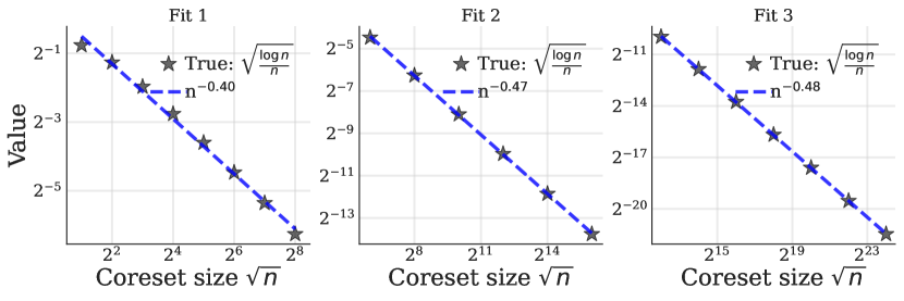
(a) True error scaling of $\sqrt{\frac{\log n}{n}}$

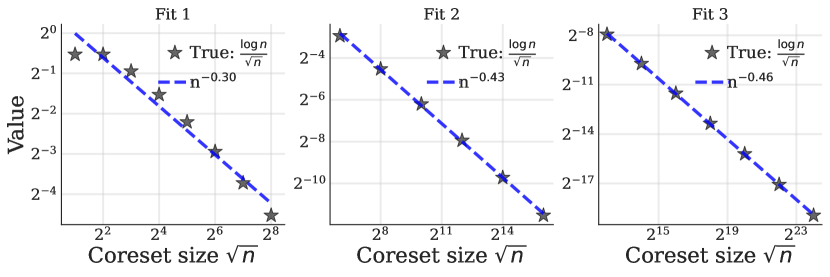
(b) True error scaling of $\frac{\log n}{\sqrt{n}}$

Figure 5: Empirical decay rates when true error $=\frac{\log^{c}n}{\sqrt{n}}$. We display the ordinary least squares fits for regressing the log of true error onto the log of input size $n$ when the true error equals either (a) $\sqrt{\frac{\log n}{n}}$ or (b) $\frac{\log n}{\sqrt{n}}$. As the input range increases, the fitted decay rate tends towards $n^{-\frac{1}{2}}$ despite appearing significantly slower for smaller input ranges.

 

P.3 MCMC vignette details

For complete details on the targets and sampling algorithms we refer the reader to Riabiz et al. [72, Sec. 4]. When applying standard thinning to any Markov chain output, we adopt the convention of keeping the final sample point. For all experiments, we used only the odd indices of the post burn-in sample points when thinning to form $\mathcal{S}_{n}$.

The selected burn-in periods for the Goodwin task were 820,000 for RW; 824,000 for adaRW; 1,615,000 for MALA; and 1,475,000 for pMALA. The respective numbers for the Lotka-Volterra task were 1,512,000 for RW; 1,797,000 for adaRW; 1,573,000 for MALA; and 1,251,000 for pMALA. For the Hinch experiments, we discard the first $10^{6}$ points as burn-in following Riabiz et al. [72, App. S5.4]. For all $n$, the parameter $\sigma$ for the Gaussian kernel is set to the median distance between all pairs of $4^{7}$ points obtained by standard thinning the post-burn-in odd indices. The resulting values for the Goodwin chains were 0.02 for RW; 0.0201 for adaRW; 0.0171 for MALA; and 0.0205 for pMALA. The respective numbers for Lotka-Volterra task were 0.0274 for RW; 0.0283 for adaRW; 0.023 for MALA; and 0.0288 for pMALA. Finally, the numbers for the Hinch task were 8.0676 for RW; 8.3189 for adaRW; 8.621 for MALA; and 8.6649 for pMALA.

Appendix Q Kernel Thinning with Square-root Dominating Kernels

As alluded to in Sec. 2, it is not necessary to identify an exact square-root kernel ${\mathbf{k}}_{\mathrm{rt}}$ to run kernel thinning. Rather, it suffices to identify any square-root dominating kernel $\widetilde{\mathbf{k}}_{\mathrm{rt}}$ defined as follows.

Definition 8 (Square-root dominating kernel).

We say a reproducing kernel $\widetilde{\mathbf{k}}_{\mathrm{rt}}:\mathbb{R}^{d}\times\mathbb{R}^{d}\to\mathbb{R}$ is a square-root dominating kernel for a reproducing kernel ${\mathbf{k}_{\star}}:\mathbb{R}^{d}\times\mathbb{R}^{d}\to\mathbb{R}$ if $\widetilde{\mathbf{k}}_{\mathrm{rt}}(x,\cdot)$ is square-integrable for all $x\in\mathbb{R}^{d}$ and either of the following equivalent conditions hold.

1. The RKHS of ${\mathbf{k}_{\star}}$ belongs to the RKHS of $\widetilde{\mathbf{k}}(x,y)\triangleq\int_{\mathbb{R}^{d}}\widetilde{\mathbf{k}}_{\mathrm{rt}}(x,z)\widetilde{\mathbf{k}}_{\mathrm{rt}}(y,z)dz$.

2. The function $\widetilde{\mathbf{k}}-c{\mathbf{k}_{\star}}$ is positive definite for some $c>0$.

Remark 9 (Controlling $\operatorname{MMD}_{{\mathbf{k}_{\star}}}$).

A square-root dominating kernel $\widetilde{\mathbf{k}}_{\mathrm{rt}}$ is a suitable surrogate for ${\mathbf{k}}_{\mathrm{rt}}$ as, by Zhang and Zhao [92, Lem. 2.2, Prop. 2.3], $\operatorname{MMD}_{{\mathbf{k}_{\star}}}(\mu,\nu)\leq\sqrt{1/c}\cdot\operatorname{MMD}_{\widetilde{\mathbf{k}}}(\mu,\nu)$ for $c$ the constant appearing in Def. 8(b) and all distributions $\mu$ and $\nu$.

Defs. 8 and 9 enable us to use convenient dominating surrogates whenever an exact square-root kernel is inconvenient to derive or deploy. For example, our next result, proved in Sec. Q.1, shows that a standard Matérn kernel is a square-root dominating kernel for every sufficiently-smooth shift-invariant and absolutely integrable ${\mathbf{k}_{\star}}$.

Proposition 4 (Dominating smooth kernels).

If ${\mathbf{k}_{\star}}(x,y)=\kappa(x-y)$ and $\kappa\in{L}^{1}\cap C^{2\nu}$ for $\nu>d$, then, for any $\gamma>0$, the Matérn$(\frac{\nu}{2},\gamma)$ kernel of Tab. 2 is a square-root dominating kernel for ${\mathbf{k}_{\star}}$.

Checking the square-root dominating condition is also particularly simple for any pair of continuous shift-invariant kernels as the next result, proved in Sec. Q.2, shows.

Proposition 5 (Dominating shift-invariant kernels).

Suppose that the real-valued kernels ${\mathbf{k}_{\star}}(x,y)=\kappa(x-y)$ and $\widetilde{\mathbf{k}}_{\mathrm{rt}}(x,y)=\widetilde{\kappa}_{\mathrm{rt}}(x-y)$ have respective spectral densities (Def. 6) $\widehat{\kappa}$ and ${\widehat{\kappa}}_{\mathrm{rt}}$. If ${\widehat{\kappa}}_{\mathrm{rt}}\in{L}^{2}$, then $\widetilde{\mathbf{k}}_{\mathrm{rt}}$ is a square-root dominating kernel for ${\mathbf{k}_{\star}}$ if and only if

$$\mathop{\mathrm{missing}}{ess\,sup}_{\omega\in\mathbb{R}^{d}:\,\widehat{\kappa}(\omega)>0}\textstyle{\frac{\widehat{\kappa}(\omega)}{{\widehat{\kappa}}_{\mathrm{rt}}(\omega)^{2}}}<\infty.$$ (358)

In Tab. 10, we use Prop. 5 to derive convenient tailored square-root dominating kernels $\widetilde{\mathbf{k}}_{\mathrm{rt}}$ for standard inverse multiquadric kernels, hyberbolic secant (sech) kernels, and Wendland’s compactly supported kernels. In each case, we can identify a square-root dominating kernel from the same family.

Name of kernel
${\mathbf{k}_{\star}}(x,y)=\kappa(x-y)$	Expression for
$\kappa(z)$	Name of square-root dominating
kernel $\widetilde{\mathbf{k}}_{\mathrm{rt}}(x,y)=\widetilde{\kappa}_{\mathrm{rt}}(x-y)$
InverseMultiquadric$(\nu,\gamma)$
$\nu>0,\gamma>0$	$(\gamma^{2}+\mathopen{}\mathclose{{}\left\|{z}}\right\|_{2}^{2})^{-\nu}$	InverseMultiquadric$(\nu^{\prime},\gamma^{\prime})$
$(\nu^{\prime},\gamma^{\prime})\in\mathcal{C}_{\nu,\gamma,d}$; see 372
Sech$(a)$
$a>0$	$\displaystyle\prod_{j=1}^{d}\textstyle\operatorname{sech}\mathopen{}\mathclose{{}\left(\sqrt{\frac{\pi}{2}}az_{j}}\right)$	Sech$(2a)$
Wendland$(s)$
$s\in\mathbb{N},s\geq\frac{1}{2}(d+1)$	$\phi_{d,s}(\mathopen{}\mathclose{{}\left\|{z}}\right\|_{2})$; see 359	Wendland$(s^{\prime})$
$s^{\prime}\in\mathbb{N}_{0},s^{\prime}\leq\frac{1}{4}(2s\!-\!1\!-d)$

arxiv

Table 9: Square-root dominating kernels $\widetilde{\mathbf{k}}_{\mathrm{rt}}$ for common kernels ${\mathbf{k}_{\star}}$ (see Def. 8). Here $\mathbb{N}_{0}$ denotes the non-negative integers. See Sec. Q.3 for our derivation.

jmlr

Table 10: Square-root dominating kernels $\widetilde{\mathbf{k}}_{\mathrm{rt}}$ for common kernels ${\mathbf{k}_{\star}}$ (see Def. 8). Here $\mathbb{N}_{0}$ denotes the non-negative integers. See Sec. Q.3 for our derivation.

Expressions for Wendland kernels

The Wendland$(s)$ kernel is a compactly-supported radial kernel $\phi_{d,s}(\mathopen{}\mathclose{{}\left\|{x-y}}\right\|_{2})$ on $\mathbb{R}^{d}$ where $\phi_{d,s}:{}_{+}\to\real$ is a truncated minimal-degree polynomial with $2s$ continuous derivatives. We collect here the expressions for $\phi_{d,s}$ for $s=0,1,2$ and refer the readers to Wendland [91, Ch. 9, Thm. 9.13, Tab. 9.1] for more general $s$. Let $(r)_{+}=\max(0,r)$ and $\ell\triangleq\lfloor{d/2}\rfloor+3$, then we have

$$\textstyle\phi_{d,0}(r) \textstyle=(1-r)_{+}^{\lfloor{d/2}\rfloor+1},\quad\phi_{d,1}(r)=(1-r)_{+}^{\lfloor{d/2}\rfloor+2}[(\lfloor{d/2}\rfloor+2)r+1]$$ (359)

$$\textstyle\phi_{d,2}(r) \textstyle=(1-r)_{+}^{\lfloor{d/2}\rfloor+3}[(\ell^{2}+4\ell+3)r^{2}+(3\ell+6)r+3].$$ (360)

Q.1 Proof of Prop. 4: Dominating smooth kernels

Since $\kappa\in{L}^{1}$, $\mathcal{F}(\kappa)$ is bounded by the Babenko-Beckner inequality [7] and nonnegative by Bochner’s theorem [10, 91, Thm. 6.6]. Moreover, since $\kappa\in C^{2\nu}$, Sun [84, Thm. 4.1] implies that $\int\mathopen{}\mathclose{{}\left\|{\omega}}\right\|_{2}^{2\nu}\mathcal{F}(\kappa)(\omega)d\omega<\infty$. By Wendland [91, Theorem 8.15], the Matérn$(\nu,\gamma)$ kernel $\widetilde{\mathbf{k}}(x,y)\propto\Phi_{\nu,\gamma}(x-y)$ for $\Phi_{\nu,\gamma}$ continuous with $\mathcal{F}(\Phi_{\nu,\gamma})(\omega)={}{(\gamma^{2}+\mathopen{}\mathclose{{}\left\|{\omega}}\right\|_{2}^{2})^{-\nu}}$. Since we have established that

$$\textstyle\int\frac{\mathcal{F}(\kappa)(\omega)^{2}}{\mathcal{F}(\Phi_{\nu,\gamma})(\omega)}d\omega\!=\!\int(\gamma^{2}+\mathopen{}\mathclose{{}\left\|{\omega}}\right\|_{2}^{2})^{\nu}\mathcal{F}(\kappa)(\omega)^{2}d\omega\!\leq\!\mathopen{}\mathclose{{}\left\|{\mathcal{F}(\kappa)}}\right\|_{\infty}\int(\gamma^{2}+\mathopen{}\mathclose{{}\left\|{\omega}}\right\|_{2}^{2})^{\nu}\mathcal{F}(\kappa)(\omega)d\omega\!<\!\infty,$$ (361)

Wendland [91, Thm. 10.12] implies that $\kappa$ belongs to $\mathcal{H}_{\widetilde{\mathbf{k}}}$ and hence that $\mathcal{H}_{{\mathbf{k}_{\star}}}\subseteq\mathcal{H}_{\widetilde{\mathbf{k}}}$. Finally, by Sec. N.1, Matérn$(\frac{\nu}{2},\gamma)$ is a valid square-root dominating kernel for $\widetilde{\mathbf{k}}$ and therefore for ${\mathbf{k}_{\star}}$.

Q.2 Proof of Prop. 5: Dominating shift-invariant kernels

Def. 6 implies that

$$\textstyle{\mathbf{k}_{\star}}(x,y)=\frac{1}{(2\pi)^{d/2}}\int e^{-i\langle{\omega},{x-y}\rangle}\widehat{\kappa}(\omega)d\omega\quad\text{and}\quad\widetilde{\mathbf{k}}_{\mathrm{rt}}(x,y)=\frac{1}{(2\pi)^{d/2}}\int e^{-i\langle{\omega},{x-y}\rangle}{\widehat{\kappa}}_{\mathrm{rt}}(\omega)d\omega,$$ (362)

Moreover, since ${\mathbf{k}}_{\mathrm{rt}}(x,\cdot)=\mathcal{F}(e^{-i\langle{\cdot},{x}\rangle}{\widehat{\kappa}}_{\mathrm{rt}})$ for $e^{-i\langle{\cdot},{x}\rangle}{\widehat{\kappa}}_{\mathrm{rt}}\in{L}^{1}\cap{L}^{2}$, the Plancherel-Parseval identity [91, Proof of Thm. 5.23] implies that

$$\textstyle\widetilde{\mathbf{k}}(x,y)\triangleq\int_{\mathbb{R}^{d}}\widetilde{\mathbf{k}}_{\mathrm{rt}}(x,z)\widetilde{\mathbf{k}}_{\mathrm{rt}}(y,z)dz \textstyle=\int_{\mathbb{R}^{d}}e^{-i\langle{\omega},{x}\rangle}{{\widehat{\kappa}}_{\mathrm{rt}}(\omega)}\ e^{i\langle{\omega},{y}\rangle}{{\widehat{\kappa}}_{\mathrm{rt}}(\omega)}d\omega$$ (363)

$$\textstyle=\int_{\mathbb{R}^{d}}e^{-i\langle{\omega},{x-y}\rangle}{\widehat{\kappa}}_{\mathrm{rt}}(\omega)^{2}d\omega,$$ (364)

and Bochner’s theorem [10, 91, Thm. 6.6] implies that $\widetilde{\mathbf{k}}$ is a kernel. Finally, Prop. 3.1 of Zhang and Zhao [92] now implies that the RKHS of ${\mathbf{k}_{\star}}$ belongs to the RKHS of $\widetilde{\mathbf{k}}$ if and only if the ratio condition 358 holds.

Q.3 Derivation of Tab. 10: Square-root dominating kernels $\widetilde{\mathbf{k}}_{\mathrm{rt}}$ for common kernels ${\mathbf{k}_{\star}}$

Thanks to Prop. 5, to establish the validity of the square root dominating kernels stated in Tab. 10, it suffices to verify that

$$\textstyle{\widehat{\kappa}}_{\mathrm{rt}}\in{L}^{2}\quad\text{and}\quad\widehat{\kappa}\precsim_{\,d,\kappa,\widetilde{\kappa}_{\mathrm{rt}}}{\widehat{\kappa}}_{\mathrm{rt}}^{2},$$ (365)

where the functions $\kappa$ and ${\widehat{\kappa}}_{\mathrm{rt}}$ are the spectral densities of $\kappa$ and $\widetilde{\kappa}_{\mathrm{rt}}$.

Inverse multiquadric

Consider the positive definite function $\Phi_{\nu,\gamma}$ 259 underlying the Matérn kernel, which is continuous on $\mathbb{R}^{d}\backslash\{{\boldsymbol{0}}\}$. When $\kappa(z)=(\gamma^{2}+\mathopen{}\mathclose{{}\left\|{z}}\right\|_{2}^{2})^{-\nu}$ and $\widetilde{\kappa}_{\mathrm{rt}}(z)=({\gamma^{\prime}}^{2}+\mathopen{}\mathclose{{}\left\|{z}}\right\|_{2}^{2})^{-\nu^{\prime}}$, Wendland [91, Theorem 8.15] implies that

$$\textstyle\widehat{\kappa}(\omega)=\Phi_{\nu,\gamma}(\omega)\quad\text{and}\quad\Phi_{\nu^{\prime},\gamma^{\prime}}^{2}(\omega)={\widehat{\kappa}}_{\mathrm{rt}}(\omega)^{2}.$$ (366)

Let $a(\omega)\asymp_{d,\nu,\gamma}b(\omega)$ denote asymptotic equivalence up to a constant depending on $d,\nu,\gamma$. Then, by [22, Eqs. 10.25.3 & 10.30.2], we have

$$\textstyle\Phi_{\nu,\gamma}(\omega) \textstyle\asymp_{d,\nu,\gamma}\mathopen{}\mathclose{{}\left\|{\omega}}\right\|_{2}^{\nu-\frac{d}{2}-\frac{1}{2}}e^{-\gamma\mathopen{}\mathclose{{}\left\|{\omega}}\right\|_{2}}\quad\text{as}\quad\mathopen{}\mathclose{{}\left\|{\omega}}\right\|_{2}\to\infty,$$ (367)

$$\textstyle\Phi_{\nu,\gamma}(\omega) \textstyle\asymp_{d,\nu,\gamma}\mathopen{}\mathclose{{}\left\|{\omega}}\right\|_{2}^{-(d-2\nu)_{+}}\quad\text{as}\quad\mathopen{}\mathclose{{}\left\|{\omega}}\right\|_{2}\to 0.$$ (368)

Hence, ${\widehat{\kappa}}_{\mathrm{rt}}\in{L}^{2}$ whenever $\nu^{\prime}>\frac{d}{4}$.

Moreover, applying 367, we find that for $\mathopen{}\mathclose{{}\left\|{\omega}}\right\|_{2}\to\infty$,

$$\textstyle\frac{\Phi_{\nu,\gamma}(\omega)}{\Phi_{\nu^{\prime},\gamma^{\prime}}^{2}(\omega)} \textstyle\asymp_{d,\nu,\gamma,\nu^{\prime},\gamma^{\prime}}\mathopen{}\mathclose{{}\left\|{\omega}}\right\|_{2}^{\nu-\frac{d}{2}-\frac{1}{2}}e^{-\gamma\mathopen{}\mathclose{{}\left\|{\omega}}\right\|_{2}}\cdot\mathopen{}\mathclose{{}\left\|{\omega}}\right\|_{2}^{-2\nu^{\prime}+d+1}e^{2\gamma^{\prime}\mathopen{}\mathclose{{}\left\|{\omega}}\right\|_{2}}$$ (369)

$$\textstyle=\mathopen{}\mathclose{{}\left\|{\omega}}\right\|_{2}^{\nu+\frac{d}{2}+\frac{1}{2}-2\nu^{\prime}}e^{(2\gamma^{\prime}-\gamma)\mathopen{}\mathclose{{}\left\|{\omega}}\right\|_{2}}.$$ (370)

If $2\gamma^{\prime}-\gamma<0$, this expression is bounded for any value of $\nu^{\prime}$. If $2\gamma^{\prime}-\gamma=0$, this expression is bounded when $\nu^{\prime}\geq\frac{\nu}{2}+\frac{d}{4}+\frac{1}{4}$.

Applying 368, we find that for $\mathopen{}\mathclose{{}\left\|{\omega}}\right\|_{2}\to 0$,

$$\textstyle\frac{\Phi_{\nu,\gamma}(\omega)}{\Phi_{\nu^{\prime},\gamma^{\prime}}^{2}(\omega)} \textstyle\asymp_{d,\nu,\gamma,\nu^{\prime},\gamma^{\prime}}\mathopen{}\mathclose{{}\left\|{\omega}}\right\|_{2}^{-(d-2\nu)_{+}}\cdot\mathopen{}\mathclose{{}\left\|{\omega}}\right\|_{2}^{2(d-2\nu^{\prime})_{+}}=\mathopen{}\mathclose{{}\left\|{\omega}}\right\|_{2}^{2(d-2\nu^{\prime})_{+}-(d-2\nu)_{+}},$$ (371)

If $\nu\geq\frac{d}{2}$, this expression is finite for any value of $\nu^{\prime}$. If $\nu<\frac{d}{2}$, this expression is finite when $\nu^{\prime}\leq\frac{\nu}{2}+\frac{d}{4}$. Hence, our condition 365 is verified whenever $(\nu^{\prime},\gamma^{\prime})$ belongs to the set

$$\textstyle\mathcal{C}_{\nu,\gamma,d}\triangleq\big{\{}(\nu^{\prime},\gamma^{\prime}):\ \textstyle(1)\ \nu^{\prime}>\frac{d}{4}\quad\text{and}\quad\gamma^{\prime}\leq\frac{\gamma}{2},\quad\text{and}\quad$$ (372)

$$\textstyle(2)\ \nu^{\prime}\leq\frac{d}{4}+\frac{\nu}{2}\quad\text{if}\quad\nu<\frac{d}{2},\quad\text{and}\quad$$ (373)

$$\textstyle(3)\ \nu^{\prime}\geq\frac{d}{4}+\frac{\nu}{2}+\frac{1}{4}\quad\text{if}\quad\gamma^{\prime}=\frac{\gamma}{2}\big{\}}.$$ (374)

Sech

Define $\kappa_{a}(z)\triangleq\prod_{j=1}^{d}\operatorname{sech}\mathopen{}\mathclose{{}\left(\sqrt{\frac{\pi}{2}}az_{j}}\right)$, and suppose $\kappa=\kappa_{a}$ and $\widetilde{\kappa}_{\mathrm{rt}}=\kappa_{2a}$. Huggins and Mackey [41, Ex. 3.2] yields that

$$\textstyle\widehat{\kappa}(\omega)=\mathcal{F}(\kappa_{a})(\omega) \textstyle=\frac{1}{a^{d}}\prod_{j=1}^{d}\operatorname{sech}(\sqrt{\frac{\pi}{2}}\frac{\omega_{j}}{a})=a^{-d}\cdot\kappa_{1/a}(\omega),\quad\text{and}\quad$$ (375)

$$\textstyle{\widehat{\kappa}}_{\mathrm{rt}}(\omega)=\mathcal{F}(\widetilde{\kappa}_{\mathrm{rt}})(\omega) \textstyle=(2a)^{-d}\kappa_{1/(2a)}(\omega).$$ (376)

Since $\operatorname{sech}^{2}(b/2)=\frac{4}{e^{b}+e^{-b}+2}>\frac{4}{e^{b}+e^{-b}}=2\operatorname{sech}(b)$, we have

$$\textstyle\kappa_{1/a}(\omega)\leq 2^{-d}\cdot\kappa_{1/(2a)}(\omega)^{2}.$$ (377)

Putting the pieces together, we further have

$$\textstyle\widehat{\kappa}(\omega)\stackrel{{\scriptstyle\lx@cref{creftype~refnum}{eq:sech_fourier}}}{{=}}a^{-d}\cdot\kappa_{1/a}(\omega)\stackrel{{\scriptstyle\lx@cref{creftype~refnum}{eq:sech_bound_kappa}}}{{\leq}}(2a)^{-d}\cdot\kappa_{1/(2a)}(\omega)^{2}\stackrel{{\scriptstyle\lx@cref{creftype~refnum}{eq:sech_fourier_sqrt}}}{{=}}(2a)^{d}\cdot{\widehat{\kappa}}_{\mathrm{rt}}(\omega)^{2}.$$ (378)

Since $\kappa_{1/(2a)}\in{L}^{2}$, we have verified the condition 365.

Wendland

When $\kappa(z)=\phi_{d,s}(\mathopen{}\mathclose{{}\left\|{z}}\right\|_{2})$ and $\widetilde{\kappa}_{\mathrm{rt}}(z)=\phi_{d,s^{\prime}}(\mathopen{}\mathclose{{}\left\|{z}}\right\|_{2})$, Wendland [91, Thm. 10.35] implies that

$$\textstyle\widehat{\kappa}(\omega)\precsim_{d,s,s^{\prime}}\frac{1}{(1+\mathopen{}\mathclose{{}\left\|{\omega}}\right\|_{2}^{2})^{d+2s+1}}\leq\frac{1}{(1+\mathopen{}\mathclose{{}\left\|{\omega}}\right\|_{2}^{2})^{2d+4s^{\prime}+2}}\precsim_{d,s,s^{\prime}}{\widehat{\kappa}}_{\mathrm{rt}}(\omega)^{2}\precsim_{d,s,s^{\prime}}\frac{1}{(1+\mathopen{}\mathclose{{}\left\|{\omega}}\right\|_{2}^{2})^{2d+4s^{\prime}+2}},$$ (379)

with $s^{\prime}\in\mathbb{N}_{0},s^{\prime}\leq\frac{(2s\!-\!1\!-d)}{4}$, thereby establishing the condition 365.

Appendix R Online Vector Balancing in Euclidean Space

Using Thm. 3, we recover the online vector balancing result of Alweiss et al. [1, Thm. 1.2] with improved constants and a less conservative setting of the thresholds $\mathfrak{a}_{i}$. Note that we capture the usual obliviousness assumption by treating the sequence $(f_{i})_{i=1}^{n}$ as a fixed, deterministic input to Alg. 5.

Corollary 7 (Online vector balancing in Euclidean space).

If $\mathcal{H}=\mathbb{R}^{d}$ equipped with the Euclidean dot product, each $\mathopen{}\mathclose{{}\left\|{f_{i}}}\right\|_{2}\leq 1$, and each $\mathfrak{a}_{i}=\frac{1}{2}+\log(4n/\delta)$, then, with probability at least $1-\delta$, the self-balancing Hilbert walk (Alg. 5) returns $\psi_{n}$ satisfying

$$\textstyle\mathopen{}\mathclose{{}\left\|{\psi_{n}}}\right\|_{\infty}=\mathopen{}\mathclose{{}\left\|{\sum_{i=1}^{n}\eta_{i}f_{i}}}\right\|_{\infty}\leq\sqrt{2\log(4d/\delta)\log(4n/\delta)}.$$ (380)

Proof.

Instantiate the notation of Thm. 3. With our choice of $\mathfrak{a}_{i}$, the signed sum representation property (ii) implies that $\psi_{n}=\sum_{i=1}^{n}\eta_{i}f_{i}$ with probability at least $1-\delta/2$. Moreover, the union bound, the functional sub-Gaussianity property (i), and the sub-Gaussian Hoeffding inequality [90, Prop. 2.5] now imply

$$\textstyle\mathrm{Pr}(\mathopen{}\mathclose{{}\left\|{\psi_{n}}}\right\|_{\infty}>t\mid\mathcal{F}_{n})\leq\sum_{j=1}^{d}\mathbb{P}(|\langle{\psi_{n}},{e_{j}}\rangle|>t\mid\mathcal{F}_{n}) \textstyle\leq 2d\exp(-t^{2}/(2\sigma_{n}^{2}))=\delta/2$$ (381)

$$\textstyle\quad\text{for}\quad t \textstyle\triangleq\sigma_{n}\sqrt{2\log(4d/\delta)}.$$ (382)

Since $\mathfrak{a}_{i}$ is non-decreasing in $i$, and ${\textstyle\frac{\frac{1}{2}+\log(4/\delta)}{\log(4/\delta)}}$ is increasing in $\delta\in(0,1]$,

$$\textstyle\sigma_{n}^{2} \textstyle=\max_{j\leq n}{\textstyle\frac{\mathfrak{a}_{j}^{2}}{2\mathfrak{a}_{j}-\|{f_{j}}\|_{\mathcal{H}}^{2}}}\leq\max_{j\leq n}{\textstyle\frac{\mathfrak{a}_{j}^{2}}{2\mathfrak{a}_{j}-1}}=\log(4n/\delta){\textstyle\frac{(\frac{1}{2}+\log(4n/\delta))^{2}}{2(\log(4n/\delta))^{2}}}$$ (383)

$$\textstyle\leq\log(4n/\delta){\textstyle\frac{(\frac{1}{2}+\log(4))^{2}}{2(\log(4))^{2}}}\leq\log(4n/\delta).$$ (384)

The advertised result now follows from the union bound. ∎

Appendix S $L^{\infty}$ Coresets of Phillips and Tai [69] and Tai [85]

Here we provide more details on the $L^{\infty}$ coreset construction of Phillips and Tai [69] and Tai [85] discussed in Sec. 8.3. Given input points $(x_{i})_{i=1}^{n}$, the Phillips-Tai (PT) construction forms the matrix $K=({\mathbf{k}_{\star}}(x_{i},x_{j}))_{i,j=1}^{n}$ of pairwise kernel evaluations, finds a matrix square-root $V\in\mathbb{R}^{n\times n}$ satisfying $K=VV^{\top}$, and augments $V$ with a row of ones (to encourage near-halving in the next step). Then, the PT construction runs the Gram-Schmidt (GS) walk of [4] to identify approximately half of the columns of $V$ as coreset members and rebalances the coreset until exactly half of the input points belong to the coreset. The GS walk and rebalancing steps are recursively repeated $\Omega(\log(n))$ times to obtain an $(n^{\frac{1}{2}},\mathcal{O}_{p}(\sqrt{d}n^{-\frac{1}{2}}\sqrt{\log n}))$-$L^{\infty}$ coreset. The low-dimensional Gaussian kernel construction of Tai [85] first partitions the input points into balls of radius $2\sqrt{\log n}$ and then applies the PT construction separately to each ball. The result is an $(n^{\frac{1}{2}},\mathcal{O}_{p}(2^{d}n^{-\frac{1}{2}}\sqrt{\log(d\log n)}))$-$L^{\infty}$ coreset with an additional superexponential $\Omega(d^{5d})$ running time dependence. RD acknowledges support by National Science Foundation under Grant No. DMS2023528 for the Foundations of Data Science Institute (FODSI). The authors thank François-Xavier Briol, Lucas Janson, Lingxiao Li, Chris Oates, Art Owen, and the anonymous reviewers for their valuable feedback on this work and Jeffrey Rosenthal for helpful discussions surrounding geometric ergodicity. Part of this work was done when RD was interning at Microsoft Research New England.

References

• Alweiss et al. [2021] Ryan Alweiss, Yang P Liu, and Mehtaab Sawhney. Discrepancy minimization via a self-balancing walk. In Proceedings of the 53rd Annual ACM SIGACT Symposium on Theory of Computing, pages 14–20, 2021.
• Augustin et al. [2016] Christoph M Augustin, Aurel Neic, Manfred Liebmann, Anton J Prassl, Steven A Niederer, Gundolf Haase, and Gernot Plank. Anatomically accurate high resolution modeling of human whole heart electromechanics: A strongly scalable algebraic multigrid solver method for nonlinear deformation. Journal of computational physics, 305:622–646, 2016.
• Bach et al. [2012] Francis Bach, Simon Lacoste-Julien, and Guillaume Obozinski. On the equivalence between herding and conditional gradient algorithms. In Proceedings of the 29th International Coference on International Conference on Machine Learning, ICML’12, page 1355–1362, Madison, WI, USA, 2012. Omnipress. ISBN 9781450312851.
• Bansal et al. [2018] Nikhil Bansal, Daniel Dadush, Shashwat Garg, and Shachar Lovett. The Gram-Schmidt walk: A cure for the Banaszczyk blues. In Proceedings of the 50th Annual ACM SIGACT Symposium on Theory of Computing, pages 587–597, 2018.
• Bardenet and Hardy [2020] Rémi Bardenet and Adrien Hardy. Monte Carlo with determinantal point processes. The Annals of Applied Probability, 30(1):368–417, 2020.
• Batir [2017] Necdet Batir. Bounds for the gamma function. Results in Mathematics, 72(1):865–874, 2017. doi: 10.1007/s00025-017-0698-0. URL https://doi.org/10.1007/s00025-017-0698-0.
• Beckner [1975] William Beckner. Inequalities in Fourier analysis. Annals of Mathematics, pages 159–182, 1975.
• Belhadji et al. [2019] Ayoub Belhadji, Rémi Bardenet, and Pierre Chainais. Kernel quadrature with DPPs. In Advances in Neural Information Processing Systems, volume 32, pages 12927–12937. Curran Associates, Inc., 2019.
• Belhadji et al. [2020] Ayoub Belhadji, Rémi Bardenet, and Pierre Chainais. Kernel interpolation with continuous volume sampling. In International Conference on Machine Learning, pages 725–735. PMLR, 2020.
• Bochner [1933] Salomon Bochner. Monotone funktionen, stieltjessche integrale und harmonische analyse. Mathematische Annalen, 108(1):378–410, 1933.
• Borodachov et al. [2014] Sergiy V Borodachov, Douglas P Hardin, and Edward B Saff. Low complexity methods for discretizing manifolds via Riesz energy minimization. Foundations of Computational Mathematics, 14(6):1173–1208, 2014.
• Borwein and Chan [2009] Jonathan M Borwein and O-Yeat Chan. Uniform bounds for the complementary incomplete gamma function. Mathematical Inequalities and Applications, 12:115–121, 2009.
• Briol et al. [2015] François-Xavier Briol, Chris J. Oates, Mark Girolami, and Michael A. Osborne. Frank-Wolfe Bayesian Quadrature: Probabilistic integration with theoretical guarantees. In Advances in Neural Information Processing Systems, pages 1162–1170, 2015.
• Brooks et al. [2011] Steve Brooks, Andrew Gelman, Galin Jones, and Xiao-Li Meng. Handbook of Markov chain Monte Carlo. CRC press, 2011.
• Buldygin and Kozachenko [1980] V. V. Buldygin and Yu. V. Kozachenko. Sub-gaussian random variables. Ukrainian Mathematical Journal, 32(6):483–489, 1980. doi: 10.1007/BF01087176. URL https://doi.org/10.1007/BF01087176.
• Campbell and Broderick [2019] Trevor Campbell and Tamara Broderick. Automated scalable Bayesian inference via Hilbert coresets. The Journal of Machine Learning Research, 20(1):551–588, 2019.
• Chen and Skriganov [2002] W WL Chen and MM Skriganov. Explicit constructions in the classical mean squares problem in irregularities of point distribution. Journal fur die Reine und Angewandte Mathematik, (545):67–95, 2002.
• Chen et al. [2018] W. Y. Chen, L. Mackey, J. Gorham, F-X. Briol, and C. J. Oates. Stein points. In Proceedings of the 35th International Conference on Machine Learning, 2018.
• Chen et al. [2019] Wilson Ye Chen, Alessandro Barp, François-Xavier Briol, Jackson Gorham, Mark Girolami, Lester Mackey, and Chris Oates. Stein point Markov chain Monte Carlo. In International Conference on Machine Learning, pages 1011–1021. PMLR, 2019.
• Chen et al. [2010] Yutian Chen, Max Welling, and Alex Smola. Super-samples from kernel herding. In Proceedings of the Twenty-Sixth Conference on Uncertainty in Artificial Intelligence, UAI’10, page 109–116, Arlington, Virginia, USA, 2010. AUAI Press. ISBN 9780974903965.
• De Marchi et al. [2005] Stefano De Marchi, Robert Schaback, and Holger Wendland. Near-optimal data-independent point locations for radial basis function interpolation. Advances in Computational Mathematics, 23(3):317–330, 2005.
• [22] DLMF. NIST Digital Library of Mathematical Functions. http://dlmf.nist.gov/, Release 1.1.1 of 2021-03-15. F. W. J. Olver, A. B. Olde Daalhuis, D. W. Lozier, B. I. Schneider, R. F. Boisvert, C. W. Clark, B. R. Miller, B. V. Saunders, H. S. Cohl, and M. A. McClain, eds.
• Douc et al. [2018] Randal Douc, Eric Moulines, Pierre Priouret, and Philippe Soulier. Markov chains. Springer, 2018.
• Durrett [2019] Rick Durrett. Probability: Theory and Examples. Cambridge Series in Statistical and Probabilistic Mathematics. Cambridge University Press, 5 edition, 2019. doi: 10.1017/9781108591034.
• Dwivedi and Mackey [2022] Raaz Dwivedi and Lester Mackey. Generalized kernel thinning. In International Conference on Learning Representations, 2022.
• Dwivedi et al. [2019] Raaz Dwivedi, Ohad N Feldheim, Ori Gurel-Gurevich, and Aaditya Ramdas. The power of online thinning in reducing discrepancy. Probability Theory and Related Fields, 174(1):103–131, 2019.
• El Karoui [2010] Noureddine El Karoui. The spectrum of kernel random matrices. The Annals of Statistics, 38(1):1–50, 2010.
• Gallegos-Herrada et al. [2023] M. A. Gallegos-Herrada, D. Ledvinka, and J. S. Rosenthal. Equivalences of geometric ergodicity of markov chains, 2023.
• Garreau et al. [2017] Damien Garreau, Wittawat Jitkrittum, and Motonobu Kanagawa. Large sample analysis of the median heuristic. arXiv preprint arXiv:1707.07269, 2017.
• Girolami and Calderhead [2011] Mark Girolami and Ben Calderhead. Riemann manifold Langevin and Hamiltonian Monte Carlo methods. Journal of the Royal Statistical Society: Series B (Statistical Methodology), 73(2):123–214, 2011.
• Goodwin [1965] Brian C Goodwin. Oscillatory behavior in enzymatic control process. Advances in Enzyme Regulation, 3:318–356, 1965.
• Graham et al. [1994] Ronald L. Graham, Donald Ervin Knuth, and Oren Patashnik. Concrete Mathematics: A Foundation for Computer Science. Addison-Wesley, Reading, MA, Second edition, 1994. URL https://www.csie.ntu.edu.tw/\~r97002/temp/Concrete\%20Mathematics\%202e.pdf.
• Gretton et al. [2012] Arthur Gretton, Karsten M. Borgwardt, Malte J. Rasch, Bernhard Schölkopf, and Alexander Smola. A kernel two-sample test. Journal of Machine Learning Research, 13(25):723–773, 2012.
• Gurumoorthy et al. [2019] Karthik S Gurumoorthy, Amit Dhurandhar, Guillermo Cecchi, and Charu Aggarwal. Efficient data representation by selecting prototypes with importance weights. In 2019 IEEE International Conference on Data Mining (ICDM), pages 260–269. IEEE, 2019.
• Haario et al. [1999] Heikki Haario, Eero Saksman, and Johanna Tamminen. Adaptive proposal distribution for random walk Metropolis algorithm. Computational Statistics, 14(3):375–395, 1999.
• Harvey and Samadi [2014] Nick Harvey and Samira Samadi. Near-optimal herding. In Conference on Learning Theory, pages 1165–1182, 2014.
• Havet et al. [2020] Antoine Havet, Matthieu Lerasle, Eric Moulines, and Elodie Vernet. A quantitative McDiarmid’s inequality for geometrically ergodic Markov chains. Electronic Communications in Probability, 25(none):1 – 11, 2020. doi: 10.1214/20-ECP286. URL https://doi.org/10.1214/20-ECP286.
• Hickernell [1998] Fred Hickernell. A generalized discrepancy and quadrature error bound. Mathematics of computation, 67(221):299–322, 1998.
• Hinch et al. [2004] Robert Hinch, JL Greenstein, AJ Tanskanen, L Xu, and RL Winslow. A simplified local control model of calcium-induced calcium release in cardiac ventricular myocytes. Biophysical journal, 87(6):3723–3736, 2004.
• Hoeffding [1963] Wassily Hoeffding. Probability inequalities for sums of bounded random variables. Journal of the American Statistical Association, 58(301):13–30, 1963.
• Huggins and Mackey [2018] Jonathan Huggins and Lester Mackey. Random feature Stein discrepancies. In Advances in Neural Information Processing Systems, pages 1899–1909, 2018.
• Huszár and Duvenaud [2012] Ferenc Huszár and David Kristjanson Duvenaud. Optimally-weighted herding is bayesian quadrature. ArXiv, abs/1408.2049, 2012.
• Joseph et al. [2015] V Roshan Joseph, Tirthankar Dasgupta, Rui Tuo, and CF Jeff Wu. Sequential exploration of complex surfaces using minimum energy designs. Technometrics, 57(1):64–74, 2015.
• Joseph et al. [2019] V Roshan Joseph, Dianpeng Wang, Li Gu, Shiji Lyu, and Rui Tuo. Deterministic sampling of expensive posteriors using minimum energy designs. Technometrics, 2019.
• Joshi et al. [2011] Sarang Joshi, Raj Varma Kommaraji, Jeff M Phillips, and Suresh Venkatasubramanian. Comparing distributions and shapes using the kernel distance. In Proceedings of the twenty-seventh annual symposium on Computational geometry, pages 47–56, 2011.
• Karnin and Liberty [2019] Zohar Karnin and Edo Liberty. Discrepancy, coresets, and sketches in machine learning. In Conference on Learning Theory, pages 1975–1993. PMLR, 2019.
• Karvonen et al. [2018] Toni Karvonen, Chris J Oates, and Simo Sarkka. A Bayes-Sard cubature method. In Advances in Neural Information Processing Systems, pages 5882–5893, 2018.
• Karvonen et al. [2019] Toni Karvonen, Motonobu Kanagawa, and Simo Särkkä. On the positivity and magnitudes of Bayesian quadrature weights. Statistics and Computing, 29(6):1317–1333, 2019.
• Khanna and Mahoney [2019] Rajiv Khanna and Michael W Mahoney. On linear convergence of weighted kernel herding. arXiv preprint arXiv:1907.08410, 2019.
• Kim et al. [2016] Been Kim, Rajiv Khanna, and Oluwasanmi O Koyejo. Examples are not enough, learn to criticize! Criticism for interpretability. Advances in neural information processing systems, 29, 2016.
• Koltchinskii and Giné [2000] Vladimir Koltchinskii and Evarist Giné. Random matrix approximation of spectra of integral operators. Bernoulli, pages 113–167, 2000.
• Lacoste-Julien et al. [2015] Simon Lacoste-Julien, Fredrik Lindsten, and Francis Bach. Sequential kernel herding: Frank-Wolfe optimization for particle filtering. In Artificial Intelligence and Statistics, pages 544–552. PMLR, 2015.
• Laurent and Massart [2000] Beatrice Laurent and Pascal Massart. Adaptive estimation of a quadratic functional by model selection. Annals of Statistics, pages 1302–1338, 2000.
• Liu and Lee [2017] Qiang Liu and Jason Lee. Black-box importance sampling. In Artificial Intelligence and Statistics, pages 952–961. PMLR, 2017.
• Lotka [1925] Alfred James Lotka. Elements of physical biology. Williams & Wilkins, 1925.
• Mak and Joseph [2018] Simon Mak and V Roshan Joseph. Support points. The Annals of Statistics, 46(6A):2562–2592, 2018.
• Meyn and Tweedie [2012] Sean P Meyn and Richard L Tweedie. Markov chains and stochastic stability. Springer Science & Business Media, 2012.
• Minh [2010] Ha Quang Minh. Some properties of gaussian reproducing kernel hilbert spaces and their implications for function approximation and learning theory. Constructive Approximation, 32(2):307–338, 2010.
• Mukherjea [1972] Arunava Mukherjea. A remark on tonelli’s theorem on integration in product spaces. Pacific Journal of Mathematics, 42(1):177–185, 1972.
• Niederer et al. [2011] Steven A Niederer, Lawrence Mitchell, Nicolas Smith, and Gernot Plank. Simulating human cardiac electrophysiology on clinical time-scales. Frontiers in Physiology, 2:14, 2011.
• Novak and Wozniakowski [2010] E Novak and H Wozniakowski. Tractability of multivariate problems, volume ii: Standard information for functionals, european math. Soc. Publ. House, Zürich, 3, 2010.
• Oates et al. [2017] Chris J Oates, Mark Girolami, and Nicolas Chopin. Control functionals for Monte Carlo integration. Journal of the Royal Statistical Society: Series B (Statistical Methodology), 79(3):695–718, 2017.
• Oates et al. [2019] Chris J Oates, Jon Cockayne, François-Xavier Briol, and Mark Girolami. Convergence rates for a class of estimators based on Stein’s method. Bernoulli, 25(2):1141–1159, 2019.
• O’Hagan [1991] Anthony O’Hagan. Bayes–Hermite quadrature. Journal of statistical planning and inference, 29(3):245–260, 1991.
• Owen [2017] Art B Owen. Statistically efficient thinning of a Markov chain sampler. Journal of Computational and Graphical Statistics, 26(3):738–744, 2017.
• Paige et al. [2016] Brooks Paige, Dino Sejdinovic, and Frank Wood. Super-sampling with a reservoir. In Proceedings of the Thirty-Second Conference on Uncertainty in Artificial Intelligence, pages 567–576, 2016.
• Phillips [2013] Jeff M Phillips. $\varepsilon$-samples for kernels. In Proceedings of the twenty-fourth annual ACM-SIAM symposium on Discrete algorithms, pages 1622–1632. SIAM, 2013.
• Phillips and Tai [2018] Jeff M Phillips and Wai Ming Tai. Improved coresets for kernel density estimates. In Proceedings of the Twenty-Ninth Annual ACM-SIAM Symposium on Discrete Algorithms, pages 2718–2727. SIAM, 2018.
• Phillips and Tai [2020] Jeff M Phillips and Wai Ming Tai. Near-optimal coresets of kernel density estimates. Discrete & Computational Geometry, 63(4):867–887, 2020.
• Rezaei and Gharan [2019] Alireza Rezaei and Shayan Oveis Gharan. A polynomial time mcmc method for sampling from continuous determinantal point processes. In International Conference on Machine Learning, pages 5438–5447. PMLR, 2019.
• Riabiz et al. [2020] Marina Riabiz, Wilson Ye Chen, Jon Cockayne, Pawel Swietach, Steven A. Niederer, Lester Mackey, and Chris J. Oates. Replication Data for: Optimal Thinning of MCMC Output, 2020. URL https://doi.org/10.7910/DVN/MDKNWM. Accessed on Mar 23, 2021.
• Riabiz et al. [2021] Marina Riabiz, Wilson Chen, Jon Cockayne, Pawel Swietach, Steven A Niederer, Lester Mackey, and Chris Oates. Optimal thinning of MCMC output. To appear: Journal of the Royal Statistical Society: Series B (Statistical Methodology), 2021.
• Roberts and Rosenthal [2004] Gareth O Roberts and Jeffrey S Rosenthal. General state space Markov chains and MCMC algorithms. Probability surveys, 1:20–71, 2004.
• Roberts and Tweedie [1996] Gareth O Roberts and Richard L Tweedie. Exponential convergence of Langevin distributions and their discrete approximations. Bernoulli, 2(4):341–363, 1996.
• Saitoh [1999] Saburou Saitoh. Applications of the general theory of reproducing kernels. In Reproducing Kernels and Their Applications, pages 165–188. Springer, 1999.
• Santin and Haasdonk [2017] Gabriele Santin and Bernard Haasdonk. Convergence rate of the data-independent p-greedy algorithm in kernel-based approximation. Dolomites Research Notes on Approximation, 10(Special_Issue), 2017.
• Schumaker [2007] Larry Schumaker. Spline functions: basic theory. Cambridge University Press, 2007.
• Shetty et al. [2022] Abhishek Shetty, Raaz Dwivedi, and Lester Mackey. Distribution compression in near-linear time. In International Conference on Learning Representations, 2022.
• Spencer [1977] Joel Spencer. Balancing games. Journal of Combinatorial Theory, Series B, 23(1):68–74, 1977.
• Sriperumbudur et al. [2010] Bharath K Sriperumbudur, Arthur Gretton, Kenji Fukumizu, Bernhard Schölkopf, and Gert RG Lanckriet. Hilbert space embeddings and metrics on probability measures. Journal of Machine Learning Research, 11(Apr):1517–1561, 2010.
• Steinwart and Christmann [2008] Ingo Steinwart and Andreas Christmann. Support vector machines. Springer Science & Business Media, 2008.
• Steinwart and Scovel [2012] Ingo Steinwart and Clint Scovel. Mercer’s theorem on general domains: On the interaction between measures, kernels, and RKHSs. Constructive Approximation, 35(3):363–417, 2012.
• Strocchi et al. [2020] Marina Strocchi, Matthias AF Gsell, Christoph M Augustin, Orod Razeghi, Caroline H Roney, Anton J Prassl, Edward J Vigmond, Jonathan M Behar, Justin S Gould, Christopher A Rinaldi, Martin J Bishop, Gernot Plank, and Steven A Niederer. Simulating ventricular systolic motion in a four-chamber heart model with spatially varying robin boundary conditions to model the effect of the pericardium. Journal of Biomechanics, 101:109645, 2020.
• Sun [1993] Xingping Sun. Conditionally positive definite functions and their application to multivariate interpolations. Journal of approximation theory, 74(2):159–180, 1993.
• Tai [2020] Wai Ming Tai. New nearly-optimal coreset for kernel density estimation. arXiv preprint arXiv:2007.08031, 2020.
• Tolstikhin et al. [2017] Ilya Tolstikhin, Bharath K Sriperumbudur, and Krikamol Muandet. Minimax estimation of kernel mean embeddings. The Journal of Machine Learning Research, 18(1):3002–3048, 2017.
• Turner et al. [2021] Paxton Turner, Jingbo Liu, and Philippe Rigollet. A statistical perspective on coreset density estimation. In International Conference on Artificial Intelligence and Statistics, pages 2512–2520. PMLR, 2021.
• Virtanen et al. [2020] Pauli Virtanen, Ralf Gommers, Travis E. Oliphant, Matt Haberland, Tyler Reddy, and SciPy 1. 0 others. SciPy 1.0: Fundamental Algorithms for Scientific Computing in Python. Nature Methods, 2020. doi: https://doi.org/10.1038/s41592-019-0686-2.
• Volterra [1926] Vito Volterra. Variazioni e fluttuazioni del numero d’individui in specie animali conviventi. 1926.
• Wainwright [2019] Martin J Wainwright. High-dimensional statistics: A non-asymptotic viewpoint, volume 48. Cambridge University Press, 2019.
• Wendland [2004] Holger Wendland. Scattered data approximation, volume 17. Cambridge university press, 2004.
• Zhang and Zhao [2013] Haizhang Zhang and Liang Zhao. On the inclusion relation of reproducing kernel hilbert spaces. Analysis and Applications, 11(02):1350014, 2013.
• Zhou [2002] Ding-Xuan Zhou. The covering number in learning theory. Journal of Complexity, 18(3):739–767, 2002.
\@add@PDF@RDFa@triples