Accuracy controlled data assimilation for parabolic problems

Abstract.

This paper is concerned with the recovery of (approximate) solutions to parabolic problems from incomplete and possibly inconsistent observational data, given on a time-space cylinder that is a strict subset of the computational domain under consideration. Unlike previous approaches to this and related problems our starting point is a regularized least squares formulation in a continuous infinite-dimensional setting that is based on stable variational time-space formulations of the parabolic PDE. This allows us to derive a priori as well as a posteriori error bounds for the recovered states with respect to a certain reference solution. In these bounds the regularization parameter is disentangled from the underlying discretization. An important ingredient for the derivation of a posteriori bounds is the construction of suitable Fortin operators which allow us to control oscillation errors stemming from the discretization of dual norms. Moreover, the variational framework allows us to contrive preconditioners for the discrete problems whose application can be performed in linear time, and for which the condition numbers of the preconditioned systems are uniformly proportional to that of the regularized continuous problem. In particular, we provide suitable stopping criteria for the iterative solvers based on the a posteriori error bounds. The presented numerical experiments quantify the theoretical findings and demonstrate the performance of the numerical scheme in relation with the underlying discretization and regularization.

1. Introduction

1.1. Background

Ever-increasing computational resources encourage considering more and more complex mathematical models for simulating or predicting physical/technological processes. However, striving for increasing quantifiable accuracy such models typically exhibit significant bias or are incomplete in that important model data or accurate constitutive laws are missing. It is all too natural to gather complementary information from data provided by also ever-improving sensor capabilities. Such a process of fusing models and data is often referred to as data assimilation which seems to originate from climatology [Dal94, LLD06]. In this context, streaming data are used to stabilize otherwise chaotic dynamical systems for prediction purposes, typically with the aid of (statistical) filtering techniques. While this is still an expanding and vibrant research area [Maj16], the notion of data assimilation is by now understood in a wider sense referring to efforts of improving quantifiable information extraction from synthesizing model-based and data driven approaches. Incompleteness of underlying models or model deficiencies could come in different forms. For instance, one could lack model data such as initial conditions, or the model involves uncalibrated coefficients represented e.g. by a parameter-dependent family of coefficients.

In this paper we focus on such a problem scenario where the physical law takes the form of a parabolic partial differential equation (PDE), in the simplest case just the heat equation in combination with a known source term. We then assume that the state of interest, a (near-)solution to this PDE, can be observed on some restricted time-space cylinder while its initial conditions are unknown. We are then interested in recovering the partially observed state on the whole time-space domain from the given information.

This problem is known to be (mildly) ill-posed. This or related problems have been treated in numerous articles. In particular, the recent work in [BO18, BIHO18] proposes a finite element method with built-in mesh-dependent regularization terms has been a primary motivation for the present paper. Moreover, similar concepts for an analogous data-assimilation problem associated with the wave equation have been applied in [BFMO21]. Considering first a semi-discretization in [BO18], the main results for a fully discrete scheme in [BIHO18] provide a priori estimates for the recovered state on a domain that excludes a small region around the location of initial data.

The results obtained in the present paper, although similar in nature, are instead based on a different approach and exhibit a few noteworthy distinctions explained below. In fact, our starting point is the formulation of a regularized estimation problem in terms of a least squares functional in an infinite-dimensional function space setting. We postpone for a moment the particular role of the regularization parameter in the present context and remark first that our approach resembles a number of other prior studies of ill-posed operator equations, that are also based on a Tikhonov regularization in terms of similar mixed variational formulations, see e.g. [BBLD15, BR18, BLO18, DHH13, MS17]. These contributions are typically formulated in more general setting (see e.g. [BR18]), covering also problems that exhibit a stronger level of ill-posedness such as the Cauchy problem for second order elliptic equations, or the backward heat equation. Although a direct comparison with these works is therefore difficult, there are noteworthy relevant conceptual links as well as distinctions that we will briefly comment on next.

For instance, in [BR18], one arrives at a similar mixed formulation as in the present paper exploiting then, however, just coercivity where, for a regularizing term $\varepsilon\|\cdot\|$, the coercivity constant decreases proportionally to the regularization parameter. The results in [BBLD15] for related numerical schemes indeed confirm a corresponding adverse dependence of error bounds on the regularization parameter. Moreover, these bounds are obtained only under additional regularity assumptions. In contrast, our approach is based on numerically realizing inf-sup stability needed to handle dual norms, resulting in the present context in $\varepsilon$-independent error estimates without any a priori additional regularity assumptions.

This hints at the perhaps main principal distinction from the above prior related work. Our guiding theme is that, how well one can solve the inverse problem, depends on the condition of the corresponding forward problem (already on an infinite-dimensional level), in the present context a parabolic initial-boundary value problem. Specifically, this requires identifying first a suitable pair $X,Y$ of (infinite-dimensional) trial- and test-spaces, for which the forward operator takes $X$ onto the dual $Y^{\prime}$ of $Y$, without imposing any “excess regularity” assumptions on the solution beyond membership to $X$. This is tantamount to a stable variational formulation of the forward problem in the sense of the Babuska-Necas Theorem. We briefly refer to this as “natural mapping properties”. Drawing on the work in [And13, RS18, SW20], the present approach is solely based on such natural mapping properties. As a consequence, the basic error analysis is independent of any data-consistency assumptions or of the regularity of solutions in the case of consistent data, which in general never occur in practice.

In summary, the guiding “general hope” is that, just exploiting natural mapping properties rather than assuming any excess regularity, should “help” minimizing the necessary amount of regularization in an inverse problem. This in turn, is intimately related to the central motivation of this paper, namely the development of efficient and certifiable numerical methods that should not rely on unverifiable assumptions. In a nutshell, for the particular problem type at hand, significant consequences of a stable variational formulation of the forward problem are: the proposed numerical solvers exhibit a favorable quantifiable performance to be commented on further below; regardless of data consistency and without imposing any regularity assumptions we derive sharp a priori error bounds that do not degrade when the regularization parameter tends to zero; there is no need for tuning parameters inside any mesh-dependent stabilization terms; we can derive computable a posteriori error bounds that are valid without any excess regularity assumptions, for arbitrary (inconsistent) data, and, in the present particular inverse problem, are independent of the regularization parameter.

However, it should be emphasized that our “general hope” could so far be realized only for the current rather mildly ill-posed problem class. The following remarks elaborate a bit more on some of the related aspects.

(i) Respecting natural mapping properties reveals, in particular, that a unique minimizer of the objective functional exists for any arbitrarily small regularization parameter and even for a vanishing regularization parameter. In fact, a least squares formulation by itself turns out to be already a sufficient regularization. However, the condition number of corresponding discrete systems may increase with decreasing regularization parameter. Our numerical experiments will shed some light on this interdependence. We use this insight to develop efficient preconditioners for the discrete problems. In fact, within the limitations of the infinite-dimensional formulation the solvers will be seen to exhibit a quasi-optimal performance for any fixed regularization parameter. Even for the mildly-ill posed problem under consideration this seems to be unprecedented in the literature. In that sense, the primary role of a non-vanishing regularization parameter for us is to facilitate a rigorous performance analysis of the iterative solver in favor of its quantitative improvement.

(ii) A stable infinite dimensional variational formulation is also an essential prerequisite for deriving rigorous a posteriori regularity-free - meaning they are valid without any excess regularity assumptions - error bounds for the recovered states. As shown later, such bounds can be used, in particular, to identify suitable stopping criteria for iterative solvers. Finally, we demonstrate some practical consequences of regularity-free computable a posteriori bounds in Section 6. We indicate their use for estimating data consistency errors as well as for choosing the regularization parameter in a way that accuracy of the results is not compromized in any essential way while enhancing solver performance.

(iii) Respecting natural mapping properties, allows us to “disentangle” discretization and regularization by studying first the intrinsic necessary “strength” of the regularization in the infinite-dimensional setting. Moreover, it turns out that additional regularization beyond the least squares formulation is not necessary on the infinite-dimensional level, persists to remain true for the proposed inf-sup stable discretizations. Choosing nevertheless a positive regularization parameter in favor of a better and rigorously founded solver performance, still requires a balanced choice so as to warrant optimal achievable accuracy of the state estimate. Our formulation reveals that the relevant balance criterion is then the achievable approximation accuracy of the trial space. Only sufficiently high regularity, typically hard to check in practice, allows one to express this quantity in terms of a uniform mesh-size. Our approach will be seen to offer more flexibility and potentially different choices of regularization parameters than those stemming from the a priori fixed mesh-dependent approach in [BO18, BIHO18] or [DHH13]. This concerns, for instance, adaptively refined meshes or higher order discretizations.

A perhaps more subtle further consequence of exploiting natural mapping properties are somewhat stronger a priori estimates than those obtained in previous works.

Of course, the robustness of our results with respect to the regularization parameter reflects the mild degree of ill-posedness of the data-assimilation problem under consideration. This cannot be expected to carry over to less stable problems in exactly the same fashion. We claim though that important elements will persist to hold, for instance, for conditionally stable problems. In particular, non-vanishing regularization parameters will then be essential and regularity-free a posteriori bounds will be all the more important for arriving at properly balanced choices in the spirit of the strategy indicated in Section 6. A detailed discussion is beyond the scope of this paper and is therefore deferred to forthcoming work.

1.2. Layout

In Section 2 we present a stable weak time-space formulation of a parabolic model problem and introduce the data assimilation problem considered in this work. Based on these findings we propose in Section 3 a regularized least squares formulation of the state estimation task. This formulation permits model as well as data errors as the recovered states are neither required to satisfy the parabolic equation exactly nor to match the data. We then derive a priori as well as a posteriori error estimates for the infinite-dimensional minimizer as well as for the minimizer over a finite dimensional trial space revealing the basic interplay between model inconsistencies, data errors, and regularization strength.

Since the “ideal” infinite-dimensional objective functional involves a dual-norm a practical numerical method needs to handle this term. We show that a proper discretization of the dual norm is tantamount to identifying a stable Fortin operator. For the given formulation of the parabolic problem this turns out to impose theoretical limitations on discretizations based on a standard second order variational formulation. Therefore we consider in Section 4 an equivalent first order system least squares formulation. Section 5 is devoted to the construction of Fortin operators for both settings. Moreover, we present in Sections 3.4 and 4.2 effective preconditioners for the iterative solution of the arising discrete problems along with suitable stopping criteria. Section 6 is devoted to numerical experiments that quantify the theoretical findings and illustrate the performance of the numerical schemes, in particular, depending on the choice of the regularization parameter which, in principal, could be chose as zero. We conclude in Section 7 with a brief discussion of several ramifications of the results, including the application of a posteriori bounds for estimating data-consistency errors.

1.3. Notations

In this work, by $C\lesssim D$ we will mean that $C$ can be bounded by a multiple of $D$, independently of parameters which C and D may depend on. Exceptions are given by the parameters $\eta$ and $\omega$ in the Carleman estimate (2.7), the polynomial degrees of various finite element spaces, and the dimension $d$ of the spatial domain $\Omega$. Obviously, $C\gtrsim D$ is defined as $D\lesssim C$, and $C\eqsim D$ as $C\lesssim D$ and $C\gtrsim D$.

For normed linear spaces $E$ and $F$, by $\mathcal{L}(E,F)$ we will denote the normed linear space of bounded linear mappings $E\rightarrow F$, and by $\mathcal{L}\mathrm{is}(E,F)$ its subset of boundedly invertible linear mappings $E\rightarrow F$. We write $E\hookrightarrow F$ to denote that $E$ is continuously embedded into $F$. For simplicity only, we exclusively consider linear spaces over the scalar field $\mathbb{R}$.

2. Problem Formulation and Preview

For a given domain $\Omega\subset\mathbb{R}^{d}$ and time-horizon $T>0$, let $I:=[0,T]$. Let $a(t;\cdot,\cdot)$ denote a bilinear form on $H^{1}_{0}(\Omega)\times H^{1}_{0}(\Omega)$ such that for any $\theta,\zeta\in H^{1}_{0}(\Omega)$, the function $t\mapsto a(t;\theta,\zeta)$ is measurable on $I$. Moreover, we assume that for almost all $t\in I$, $a(t;\cdot,\cdot)\colon H^{1}_{0}(\Omega)\times H^{1}_{0}(\Omega)\to\mathbb{R}$ is bounded and coercive, i.e.

(2.1) $$|a(t;\theta,\zeta)| \lesssim\|\theta\|_{H^{1}(\Omega)}\|\zeta\|_{H^{1}(\Omega)}\quad (\theta,\zeta\in H^{1}_{0}(\Omega)),$$

(2.2) $$a(t;\theta,\theta) \gtrsim\|\theta\|_{H^{1}(\Omega)}^{2}\quad (\theta\in{H^{1}_{0}(\Omega)}),$$

hold with constants independent of $t\in I$. By Lax Milgram’s Theorem, $A(t)$, defined by $(A(t)\theta)(\zeta):=a(t;\theta,\zeta)$, ($\theta,\,\zeta\in H^{1}_{0}(\Omega)$), belongs to $\mathcal{L}\mathrm{is}(H^{1}_{0}(\Omega),H^{-1}(\Omega))$.

Before discussing the parabolic data assimilation problem, we recall some facts about a time-space variational formulation of the parabolic initial value problem – the corresponding forward problem – of the form

(2.3) $$\left\{\begin{array}[]{rl}\frac{dz}{dt}(t)+A(t)z(t)&\!\!\!=h(t)\quad(t\in I\text{ a.e.}),\\ \gamma_{0}z&\!\!\!=z_{0},\end{array}\right.$$

with trace map $\gamma_{t}\colon z\mapsto z(t)$. With the spaces

$$X:=L_{2}(I;H^{1}_{0}(\Omega))\cap H^{1}(I;H^{-1}(\Omega)),\quad Y:=L_{2}(I;H^{1}_{0}(\Omega)),$$

the operator $B$ defined by

$$(Bw)(v):=\int_{I}{\textstyle\frac{dw}{dt}}(t)(v(t))+a(t;w(t),v(t))dt,$$

belongs to $\mathcal{L}(X,Y^{\prime})$. Recall also that

(2.4) $$X\hookrightarrow C(I;L_{2}(\Omega))$$

with the latter space being equipped with the norm on $L_{\infty}(I;L_{2}(\Omega)).$ In particular, this implies that $\gamma_{t}\in\mathcal{L}(X,L_{2}(\Omega))$, with a norm that is uniformly bounded in $t\in I$. The resulting weak formulation of (2.3) reads as

$$Bz=h,\quad\gamma_{0}z=z_{0},$$

and it is known (e.g. see [DL92, Ch.XVIII, §3], [Wlo82, Ch. IV, §26], [SS09]) to be well-posed in the sense that

(2.5) $$\left[\begin{array}[]{@{}c@{}}B\\ \gamma_{0}\end{array}\right]\in\mathcal{L}\mathrm{is}(X,Y^{\prime}\times L_{2}(\Omega)).$$

Turning to the data assimilation problem, suppose in what follows that $\omega\subset\Omega$ is a fixed non-empty sub-domain (possibly much smaller than $\Omega$) and that we are given data $f\in L_{2}(I\times\omega)$ as well as $g\in Y^{\prime}$. The data-assimilation problem considered in this paper is to seek a state $u\in X$, that approximately satisfies $Bu=g$, while also closely agreeing with $f$ in $L_{2}(I\times\omega)$, see [BO18, BIHO18]. To make this precise, ideally one would like to solve

(2.6) $$\left\{\begin{array}[]{rl}\frac{du}{dt}(t)+A(t)u(t)&\!\!\!=g(t)\quad(t\in I\text{ a.e.}),\\ u(t)|_{\omega}&\!\!\!=f(t)\quad(t\in I).\end{array}\right.$$

However, in general such data ${(g,f)}$ may be inconsistent, i.e., (2.6) has no solution and is therefore ill-posed. To put this formally, denoting by $\Gamma_{\omega}$ the restriction of a function on $I\times\Omega$ to a function on $I\times\omega$, we have $\Gamma_{\omega}\in\mathcal{L}(X,L_{2}(I\times\omega))$, i.e., $\Gamma_{\omega}$ is bounded on $X$. However, the range of the operator

$$B_{\omega}:=\left[\begin{array}[]{@{}c@{}}B\\ \Gamma_{\omega}\end{array}\right]\in\mathcal{L}(X,Y^{\prime}\times L_{2}(I\times\omega))$$

induced by (2.6), is a strict subset of $Y^{\prime}\times L_{2}(I\times\omega)$.

Before addressing this issue, it is instructive to understand the case of a consistent pair $(g,f)\in\operatorname{ran}B_{\omega}$, i.e., when there exists a $u\in X$ such that $(g,f)=(Bu,\Gamma_{\omega}u)$.

Remark 2.1.

Any data consistent pair $(g,f)\in\operatorname{ran}B_{\omega}$ determines a unique state $u\in X$ satisfying (2.6).

That this is indeed the case can be derived from the following crucial tool that has been employed in prior related studies such as [BO18, BIHO18] and will be heavily used in what follows as well. For $\eta\in(0,T)$ let

$$X_{\eta}:=L_{2}([\eta,T];H^{1}_{0}(\Omega))\cap H^{1}([\eta,T];H^{-1}(\Omega)).$$

Fixing both $\eta$ and a subdomain $\omega\subset\Omega$, a version of the so-called Carleman Estimate says in the present terms

(2.7) $$\|w\|_{X_{\eta}}\lesssim\|{\Gamma_{\omega}}w\|_{L_{2}(I\times\omega)}+\|Bw\|_{Y^{\prime}}\quad(w\in X).$$

Remark 2.2.

The validity of (2.7) has been established in [BO18, Thm. 2] for the heat operator (i.e., $a(t;\theta,\zeta)=\int_{\Omega}\nabla\theta(t)\cdot{\nabla}\zeta(t)\,d{\bf x}$) and $\Omega\subset\mathbb{R}^{d}$ being a convex polytope. It holds in greater generality though. For instance, the argument in the proof of [BO18, Lemma 7] still works when $\Omega$ is star-shaped w.r.t. an $x_{0}\in\Omega$ and any open $\omega\subset\Omega$ that contains $x_{0}$. In what follows up to this point we will tacitly assume at this point suitable problem specifications that guarantee the validity of (2.7) without further mentioning.

Returning to the uniqueness of $u$ given consistent data ${(g,f)}$, suppose there exist two solutions, then their difference $e\in X$ satisfies $\|{\Gamma_{\omega}}e\|_{L_{2}(I\times\omega)}+\|Be\|_{Y^{\prime}}=0$, meaning in view of (2.7) that $\|e\|_{X_{\eta}}=0$, and so thanks to $X_{\eta}\hookrightarrow C([\eta,T];L_{2}(\Omega))$, that $e(t)=0$ for $t\in[\eta,T]$. From $X\hookrightarrow C([0,T];L_{2}(\Omega))$, and the fact that $\eta>0$ is arbitrary, it follows that $e=0$.

However, the nature of the Carleman Estimate indicates that one cannot stably recover the trace $\gamma_{0}u$ which would then together with $g$ stably recover $u$. In fact, one may convince oneself that significantly different initial data (far) outside $\omega$ may give rise to homogeneous solutions of (2.3) that hardly differ on $I\times\omega$. Thus, even for a state $u\in X$ from (nearly) consistent data ${(g,f)\in Y^{\prime}\times L_{2}(I\times\omega)}$ we cannot expect to find an accurate numerical approximation to $u$ on the whole time-space cylinder $I\times\Omega$. Moreover, any perturbation of the data may land outside $\operatorname{ran}B_{\omega}$.

In practice, neither will the data/measurements $(g,f)\in Y^{\prime}\times L_{2}(I\times\omega)$ be exact, nor will the observed state behind $f$ satisfy the model – here a parabolic PDE – exactly. Thus, in general a pair of data $(g,f)\in Y^{\prime}\times L_{2}(I\times\omega)$ allows one to recover any hypothetical source $u\in X$ only within some uncertainty. A central theme in this article is to quantify this uncertainty (theoretically and numerically) by properly exploiting the information provided by the PDE model, and the data. While any such assimilation attempt rests on the basic hypothesis that the data ${(g,f)}$ are “close” in ${Y^{\prime}\times L_{2}(I\times\omega)}$ to a consistent pair $(Bu,u|_{I\times\omega})\in\operatorname{ran}\,B_{\omega}$, for some $u\in X$, this “closeness” is generally not known beforehand.

To perform such a recovery we formulate in the next section a family of regularizations of the ill-posed problem (2.6) involving a parameter $\varepsilon\geq 0$, taking data errors and model bias into account. We then show, first on the continuous infinite-dimensional level, that for each $\varepsilon\geq 0$ there exists a unique regularized solution $u_{\varepsilon}\in X$. Letting this precede an actual discrete scheme, will be important for a number of issues, such as the design of efficient iterative solvers, the derivation of a posteriori error bounds, as well as disentangling regularization and discretization in favor of an overall good balance of uncertainties. Aside from the question what a preferable choice of $\varepsilon$ would be in that latter respect, a central issue will be to assess the quality of a regularized state $u_{\varepsilon}$ and of its approximation $u^{\delta,\delta}_{\varepsilon}$ from a given finite-dimensional trial space $X^{\delta}\subset X$ provided by our numerical scheme.

To that end, recall that generally (for inconsistent data) the idealized assimilation problem (2.6) has no solution. So whatever state $u\in X$ may be used to “explain” the data, should be viewed as a candidate or reference state that is connected with the recovery task through the consistency error

(2.8) $$e_{\rm cons}(u):={\sqrt{\|Bu-g\|^{2}_{Y^{\prime}}+\|\Gamma_{\omega}u-f\|^{2}_{L_{2}(I\times\omega)}}}.$$

At the heart of our analysis is then an a priori estimate of the type

(2.9) $$\|u-u_{\varepsilon}^{\delta,\delta}\|_{X_{\eta}}\lesssim{e_{\rm cons}(u)}+{e^{\delta}_{\rm approx}(u)}+\varepsilon\|\gamma_{0}u\|_{L_{2}(\Omega)},$$

where $e^{\delta}_{\rm approx}(u)$ denotes the error of the best approximation to $u$ from $X^{\delta}$ in $X$, thereby implicitly quantifying the regularity of the state $u$. Recall that, as always, the constant in this estimate absorbed by the $\lesssim$-symbol may depend on $\eta>0$, but neither on $u$ nor on $\varepsilon$.

It is important to note that (2.9) is valid for any $u\in X$, not making use of the assumption that $({\color[rgb]{0,0,0}{B}}u,\Gamma_{\omega}{u})$ be close to $(g,f)$. It is of evident value, of course, for states $u$ with small or at least moderate consistency error. This suggests singling out a particular state

$${u_{0}:=\operatorname*{argmin}_{u\in X}e_{\rm cons}(u)}$$

that minimizes the consistency error. As in the case of consistent data, we will see that $u_{0}$ is unique, and, and as is suggested by its notation, it will turn out to be the limit for $\varepsilon\downarrow 0$ of the regularized solutions $u_{\varepsilon}$ that will be defined later. One reason for not confining the error estimates – or perhaps better termed distance estimates – to the specific state ${u_{0}}$ is the potential significant model bias. In fact, we view it as a strength to keep (2.9) general since this covers automatically various somewhat specialized scenarios. For instance, if the data were exact, i.e., ${e_{\rm cons}(u_{0})=0}$, (2.9), for $u=u_{0}$, shows the dependence of the error just on $\varepsilon$ and the choice of the discretization. Moreover, if the model is exact (or the model bias is negligible compared with data accuracy) it will later be seen how to get a “nearly-computable” bound for ${e_{\rm cons}(u_{0})}$ and hence an idea of the model bias (due to $g$) and measurement errors in $f$. Another case of interest is $u=u_{\varepsilon}$ because this is the “compromise-solution” suggested by the chosen regularization and targeted by the numerical scheme.

Finally, while in principle, $\varepsilon$ can be chosen as small as we wish (even zero), it will be seen to benefit solving the discrete problems by choosing $\varepsilon$ as large as possible so as to remain just dominated, ideally, by $e_{\rm cons}(u_{0})$, in practice, by the announced a posteriori bounds.

3. Regularized least squares

Knowing that the data assimilation problem is ill-posed and taking the preceding considerations into account, we consider for some parameter $\varepsilon\geq 0$ the regularized least squares problem of finding the minimizer $u_{\varepsilon}$ over $X$ of

(3.1) $$G_{\varepsilon}\colon w\mapsto\|Bw-g\|_{Y^{\prime}}^{2}+\|\Gamma_{\omega}w-f\|_{L_{2}(I\times\omega)}^{2}+\varepsilon^{2}\|\gamma_{0}w\|_{L_{2}(\Omega)}^{2},$$

where, as before, $\Gamma_{\omega}$ is the restriction of a function on $I\times\Omega$ to a function on $I\times\omega$. The resulting Euler-Lagrange equations read as

(3.2) $$\langle Bu_{\varepsilon}\!-\!g,Bw\rangle_{Y^{\prime}}\!+\!\langle\Gamma_{\omega}u_{\varepsilon}\!-\!f,\Gamma_{\omega}w\rangle_{L_{2}(I\times\omega)}\!+\!\varepsilon^{2}\langle\gamma_{0}u_{\varepsilon},\gamma_{0}w\rangle_{L_{2}(\Omega)}=0\quad(w\in X).$$

Since $\Gamma_{\omega}\in\mathcal{L}(X,L_{2}(I\times\omega))$, and on account of (2.5), for $w\in X$ it holds that

(3.3) $$\varepsilon^{2}\|w\|_{X}^{2}\lesssim\|Bw\|_{Y^{\prime}}^{2}+\|\Gamma_{\omega}w\|_{L_{2}(I\times\omega)}^{2}+\varepsilon^{2}\|\gamma_{0}w\|_{L_{2}(\Omega)}^{2}\lesssim\max(1,\varepsilon^{2})\|w\|_{X}^{2}.$$

By the Lax-Milgram Lemma, we thus know that for $\varepsilon>0$ the minimizer $u_{\varepsilon}$ exists uniquely, and satisfies

(3.4) $$\|u_{\varepsilon}\|_{X}\lesssim\max(\varepsilon^{-1},1)\big{(}\|g\|_{Y^{\prime}}+\|f\|_{L_{2}(I\times\omega)}\big{)}.$$

Selecting any reference state $u\in X$, similarly to (3.4) one can show that for $\varepsilon>0$

$$\|u-u_{\varepsilon}\|_{X}\lesssim\max(\varepsilon^{-1},1)\big{(}\varepsilon\|\gamma_{0}u\|_{L_{2}(\Omega)}+{e_{\rm cons}(u)}\big{)},$$

see (2.8). This result is by no means satisfactory. With the aid of (2.7), much better bounds will be established for $\|u-u_{\varepsilon}\|_{X_{\eta}}$.

Remark 3.1.

Also for $\varepsilon=0$, the minimizer $u_{0}$ of $G_{0}(\cdot)={e_{\rm cons}(\cdot)^{2}}$ over $X$ exists uniquely. Indeed, suppose there are two minimizers. Then, by (3.2), their difference $e_{0}$ satisfies

$$\langle Be_{0},Bw\rangle_{Y^{\prime}}+\langle\Gamma_{\omega}e_{0},\Gamma_{\omega}w\rangle_{L_{2}(I\times\omega)}=0\quad(w\in X),$$

and so $\|\Gamma_{\omega}e_{0}\|^{2}_{L_{2}(I\times\omega)}+\|Be_{0}\|^{2}_{Y^{\prime}}=0$. As we have seen, using (2.4) and (2.7) this implies $e_{0}=0$.

A frequently used tool reads as follows.

Lemma 3.2.

For any $w\in X$ one has

$$\|u-w\|_{X_{\eta}}\lesssim\sqrt{G_{{0}}(w)}+{e_{\rm cons}(u)}.$$

Proof.

We infer from (2.7) and a triangle-inequality for the norm $\sqrt{\|\,\|_{L_{2}(I\times\omega)}^{2}+\|\,\|_{Y^{\prime}}^{2}}$ that

$$\|u-w\|_{X_{\eta}}\lesssim\sqrt{\|\Gamma_{\omega}(u-w)\|_{L_{2}(I\times\omega)}^{2}+\|B(u-w)\|_{Y^{\prime}}^{2}}\leq\sqrt{G_{0}(w)}+e_{\rm cons}(u)$$

which confirms the claim. ∎

When taking as reference state $u=u_{\varepsilon}$, we obtain the following a posteriori bound.

Proposition 3.3.

For $\varepsilon\geq 0$ and $w\in X$, one has

$$\|u_{\varepsilon}-w\|_{X_{\eta}}\lesssim\sqrt{G_{\varepsilon}(w)}.$$

Proof.

The proof follows from Lemma 3.2 and

$$\sqrt{G_{0}(w)}+e_{\rm cons}({\color[rgb]{0,0,0}{u_{\varepsilon}}})\leq\sqrt{G_{\varepsilon}(w)}+\sqrt{G_{\varepsilon}(u_{\varepsilon})}\leq 2\sqrt{G_{\varepsilon}(w)}.\qed$$

The same arguments, used to show for $\varepsilon\geq 0$ existence and uniqueness of the minimizer $u_{\varepsilon}$ of $G_{\varepsilon}$ over $X$, show for any closed subspace $X^{\delta}\subset X$ uniqueness of the minimizer $u^{\delta}_{\varepsilon}$ of $G_{\varepsilon}$ over $X^{\delta}$. An a priori bound for $\|u-u_{\varepsilon}^{\delta}\|_{X_{\eta}}$ for an arbitrary reference state $u\in X$ is given in the next proposition.

Proposition 3.4.

It holds that

$$\|u-u_{\varepsilon}^{\delta}\|_{X_{\eta}} \lesssim{e_{\rm cons}(u)}+{e_{{\rm approx}}^{\delta}(u)}+\varepsilon\|\gamma_{0}u\|_{L_{2}(\Omega)},$$

where

$$e^{\delta}_{\rm approx}(u):=\min_{w\in X^{\delta}}\|u-w\|_{X}$$

denotes the corresponding approximation error of the state $u$.

Proof.

Let $P_{X^{\delta}}$ denote the $X$-orthogonal projector onto $X^{\delta}$, then using $B\in\mathcal{L}(X,Y^{\prime})$ and (2.4), we infer that

$${\sqrt{G_{0}(u^{\delta}_{\varepsilon})}\leq} \sqrt{G_{\varepsilon}(u^{\delta}_{\varepsilon})}\leq\sqrt{G_{\varepsilon}(P_{X^{\delta}}u)}$$

$${\leq} \|B(u-P_{X^{\delta}}u)\|_{Y^{\prime}}+\|Bu-g\|_{Y^{\prime}}+\|f-\Gamma_{\omega}u\|_{L_{2}(I\times\omega)}+$$

$$\|\Gamma_{\omega}(u-P_{X^{\delta}}u)\|_{L_{2}(I\times\omega)}+\varepsilon\|\gamma_{0}(u-P_{X^{\delta}}u)\|_{L_{2}(\Omega)}+\varepsilon\|\gamma_{0}u\|_{L_{2}(\Omega)}$$

$$\lesssim {e_{{\rm approx}}^{\delta}(u)}+{e_{\rm cons}(u)}+\varepsilon\|\gamma_{0}u\|_{L_{2}(\Omega)},$$

which together with Lemma 3.2 completes the proof. ∎

At this point we note that because of the presence of the dual norm $\|\cdot\|_{Y^{\prime}}$ in $G_{\varepsilon}$, neither $u_{\varepsilon}^{\delta}$ nor the a posteriori bound for $\|u_{\varepsilon}-w\|_{X_{\eta}}$ from Proposition 3.3 for e.g. $w=u_{\varepsilon}^{\delta}$ can be computed. Both problems are going to be tackled in the next two subsections.

Remark 3.5.

Although the upper bound from Proposition 3.4 is minimal for $\varepsilon=0$, a reason for nevertheless taking $\varepsilon>0$, say of the order of the expected magnitude of ${e_{\rm cons}(u)+e_{{\rm approx}}^{\delta}(u)}$, is to enhance the numerical stability of solving the Euler-Lagrange equations.

Remark 3.6.

Notice that even when $e_{\rm cons}(u)=0$ and $\varepsilon=0$, Proposition 3.4 does not show that $u_{0}^{\delta}$ is a quasi-best approximation to $u$ from $X^{\delta}$. Indeed the norm $\|\cdot\|_{X}$ used to define $e^{\delta}_{\rm approx}(u)$ differs from the norm $\|\cdot\|_{X_{\eta}}$ in which $u-u_{0}^{\delta}$ is measured.

We conclude this section with a few comments on the behavior of $u_{\varepsilon}$ when $\varepsilon$ tends to zero. First, note that the consistency error of $u_{\varepsilon}$ approaches the minimal consistency error $e_{\rm cons}(u_{0})$ when $\varepsilon\to 0$ because

$$e_{\rm cons}(u_{\varepsilon})\leq\sqrt{G_{\varepsilon}(u_{\varepsilon})}\leq\sqrt{G_{\varepsilon}({u_{0}})}\,{\leq}\,{e_{\rm cons}(u_{0})}+\varepsilon\|\gamma_{0}{u_{0}}\|_{L_{2}(\Omega)}.$$

In particular, a first trivial consequence of Proposition 3.4 is that, for consistent and exact data, i.e., ${e_{\rm cons}(u_{0})}=0$, $u_{\varepsilon}$ tends to the state ${u_{0}}$ in $X_{\eta}$ for any $\eta>0$. Even without the assumption $e_{\rm cons}(u_{0})=0$, a stronger result is derived in the following remark.

Remark 3.7.

One has

$$\|{u_{0}}-u_{\varepsilon}\|_{X}\to 0,\quad\varepsilon\to 0.$$

Proof.

We remark first that $\sqrt{{G_{\varepsilon}}}$ $\,\Gamma$-converges to $\sqrt{{G_{0}}}=:F$. In fact, let $(\varepsilon_{n})_{n\in\mathbb{N}}$ tend to zero. The functionals $F_{n}:=\sqrt{{G_{\varepsilon_{n}}}}:X\to\mathbb{R}_{+}$ are uniformly coercive (in the sense of optimization, meaning that $F_{n}(w)\to\infty$ for $\|w\|_{X}\to\infty$). Let $(w_{n})_{n\in\mathbb{N}}$ be any sequence in $X$ with limit $w\in X$. Then

$$F(w)-F_{{n}}(w_{n}) \leq F(w)-F(w_{n}){\leq\sqrt{\|B(w-w_{n})\|_{Y^{\prime}}^{2}+\|\gamma_{\omega}(w-w_{n})\|_{L_{2}(I\times\omega)}^{2}}}$$

$$\lesssim\|w-w_{n}\|_{X},\quad n\in\mathbb{N},$$

so that $F(w)\leq\liminf_{n\to\infty}F_{n}(w_{n})$. Moreover, for any $w\in X$ there exists a sequence $(w_{n})_{n\in\mathbb{N}}$ in $X$ such that $F(w)\geq\limsup_{n\to\infty}F_{n}(w_{n})$, as can be seen by simply taking $w_{n}=w$. Thus, by the main Theorem of $\Gamma$-convergence, minimizers of $F_{n}$ converge to the minimizer of $F$. ∎

Thus, trying to solve the regularized problem, with $\varepsilon$ as small as possible incidentally favors ${u_{0}}$ as a target state. Thus, it is of interest to estimate $e_{\rm cons}(u_{0})$ (see Corollary 3.14 later below) since a relatively large $e_{\rm cons}(u_{0})$ weakens the relevance of $u_{0}$, favoring correspondingly larger regularization parameters.

3.1. Discretizing the dual norm

Minimizing $G_{\varepsilon}$ over $X^{\delta}$ does not correspond to a practical method because the dual norm $\|\cdot\|_{Y^{\prime}}$ cannot be evaluated. Therefore, given a family of finite dimensional subspaces $(X^{\delta})_{\delta\in\Delta}$ of $X$, the idea is to find a family $(Y^{\delta})_{\delta\in\Delta}$ of finite dimensional subspaces of $Y$, ideally with $\dim Y^{\delta}\lesssim\dim X^{\delta}$, such that $\|Bw\|_{Y^{\prime}}$ can be controlled for $w\in X^{\delta}$ by the computable quantity $\|Bw\|_{{Y^{\delta}}^{\prime}}$. This is ensured whenever

(3.5) $$\inf_{\delta\in\Delta}\inf_{{\{w\in X^{\delta}\colon Bw\neq 0\}}}\ \sup_{0\neq\mu\in Y^{\delta}}\frac{(Bw)(\mu)}{\|Bw\|_{Y^{\prime}}\|\mu\|_{Y}}>0$$

is valid.

In the subsequent discussion we make heavy use of the Riesz isometry $R\in\mathcal{L}\mathrm{is}(Y,Y^{\prime})$, defined by

$$(Rv)(w):=\langle v,w\rangle_{Y}:=\int_{I}\int_{\Omega}\nabla_{\bf x}v\cdot\nabla_{\bf x}{\color[rgb]{0,0,0}{w}}\,d{\bf x}\,dt,\quad(v,w\in Y).$$

Introducing auxiliary variables for $\mu_{\varepsilon}=R^{-1}(g-Bu_{\varepsilon})\in Y$, $\theta_{\varepsilon}=f-\Gamma_{\omega}u_{\varepsilon}\in L_{2}(I\times\omega)$, and $\nu_{\varepsilon}={-}\gamma_{0}u_{\varepsilon}\in L_{2}(\Omega)$ gives rise to a mixed formulation of the problem of finding the minimizer $u_{\varepsilon}$ over $X$ of $G_{\varepsilon}$ defined in (3.1) in terms of the saddle point system

(3.6) $$S_{\varepsilon}(\mu_{\varepsilon},\theta_{\varepsilon},\nu_{\varepsilon},u_{\varepsilon}):=\left[\begin{array}[]{@{}cccc@{}}R&0&0&B\\ 0&I&0&\Gamma_{\omega}\\ 0&0&I&\varepsilon\gamma_{0}\\ B^{\prime}&\Gamma_{\omega}^{\prime}&\varepsilon\gamma_{0}^{\prime}&0\end{array}\right]\left[\begin{array}[]{@{}c@{}}\mu_{\varepsilon}\\ \theta_{\varepsilon}\\ \nu_{\varepsilon}\\ u_{\varepsilon}\end{array}\right]=\left[\begin{array}[]{@{}c@{}}g\\ f\\ 0\\ 0\end{array}\right].$$

(see [CDW12, Sect. 2.2]). (Equivalently, (3.6) characterizes the critical point of the Lagrangian obtained when inserting in $G_{\varepsilon}$ these variables and appending corresponding constraints by Lagrange multipliers.)

Remark 3.8.

Eliminating the second and third variable from (3.6), one arrives at the equivalent more compact formulation

$$\left[\begin{array}[]{@{}cc@{}}R&B\\ B^{\prime}&-(\Gamma_{\omega}^{\prime}\Gamma_{\omega}+\varepsilon^{2}\gamma_{0}^{\prime}\gamma_{0})\end{array}\right]\left[\begin{array}[]{@{}c@{}}{\mu_{\varepsilon}}\\ {u_{\varepsilon}}\end{array}\right]=\left[\begin{array}[]{@{}c@{}}g\\ -\Gamma_{\omega}^{\prime}f,\end{array}\right]$$

It serves in Section 3.4 as the starting point for a numerical scheme.

Theorem 3.9.

Let (3.5) be valid. For $u_{\varepsilon}^{\delta,\delta}$ denoting the (unique) minimizer over $X^{\delta}$ of

$$G^{\delta}_{\varepsilon}:=w\mapsto\|Bw-g\|_{{Y^{\delta}}^{\prime}}^{2}+\|\Gamma_{\omega}w-f\|_{L_{2}(I\times\omega)}^{2}+\varepsilon^{2}\|\gamma_{0}w\|_{L_{2}(\Omega)}^{2},$$

one has

$$\|u-u^{\delta,\delta}_{\varepsilon}\|_{X_{\eta}}\lesssim{e_{\rm cons}(u)+e^{\delta}_{\rm approx}(u)}+\varepsilon\|\gamma_{0}u\|_{L_{2}(\Omega)}.$$

(We recall that, as always, the constant absorbed by the $\lesssim$-symbol may (actually will) depend on $\omega$ and $\eta$, but not on $\varepsilon\geq 0$ or $\delta\in\Delta$.)

Proof.

Denoting the block-diagonal operator comprized of the leading $3\times 3$ block in $S_{\varepsilon}$ by $D$, the operator $S_{\varepsilon}$ can be rewritten as

$$S_{\varepsilon}=\left[\begin{array}[]{@{}cc@{}}D&C_{\varepsilon}\\ C_{\varepsilon}^{\prime}&0\end{array}\right],$$

where $C_{\varepsilon}\in\mathcal{L}\big{(}X,Y^{\prime}\times L_{2}(I\times\omega)\times L_{2}(\Omega)\big{)}$ is defined by

$$(C_{\varepsilon}w)(\mu,\theta,\nu):=(Bw)(\mu)+\langle\Gamma_{\omega}w,\theta\rangle_{L_{2}(I\times\omega)}+\varepsilon\langle\gamma_{0}w,\nu\rangle_{L_{2}(\Omega)}.$$

With the usual identification of $L_{2}(I\times\omega)$ and $L_{2}(\Omega)$ with their duals, $D$ is just the isometric Riesz isomorphism between $Y\times L_{2}(I\times\omega)\times L_{2}(\Omega)$ and its dual. Equipping $X$ with the ($\varepsilon$-dependent) “energy”-norm

$$|\!|\!|w|\!|\!|_{\varepsilon}:=\sqrt{\|Bw\|_{Y^{\prime}}^{2}+\|\Gamma_{\omega}w\|_{L_{2}(I\times\omega)}^{2}+\varepsilon^{2}\|\gamma_{0}w\|_{L_{2}(\Omega)}^{2}},$$

one verifies that $\|\mathcal{C}_{\varepsilon}w\|_{Y^{\prime}\times L_{2}(I\times\omega)\times L_{2}(\Omega)}=|\!|\!|w|\!|\!|_{\varepsilon}$, so that in particular $C_{\varepsilon}$ satisfies an ‘inf-sup’ condition. Consequently, the operator $S_{\varepsilon}$ on the left hand side of (3.6) is a boundedly invertible mapping from $Y\times L_{2}(I\times\omega)\times L_{2}(\Omega)\times(X,|\!|\!|\,|\!|\!|_{\varepsilon})$ to its dual (uniformly in $\varepsilon$).

Analogously to the continuous case, the minimizer $u^{\delta,\delta}_{\varepsilon}$ of $G^{\delta}_{\varepsilon}$ equals the fourth component of the solution $(\mu^{\delta,\delta}_{\varepsilon},\theta^{\delta,\delta}_{\varepsilon},\nu^{\delta,\delta}_{\varepsilon},u^{\delta,\delta}_{\varepsilon})$ of the Galerkin discretization of (3.6) with trial space $Y^{\delta}\times L_{2}(I\times\omega)\times L_{2}(\Omega)\times X^{\delta}$. Thanks to (3.5), for $w\in X^{\delta}$ we have

$$\sup_{0\neq(\tilde{\mu},\tilde{\theta},\tilde{\nu})\in Y^{\delta}\times L_{2}(I\times\omega)\times L_{2}(\Omega)}\frac{(Bw)(\tilde{\mu})+\langle\Gamma_{\omega}w,\tilde{\theta}\rangle_{L_{2}(I\times\omega)}+\varepsilon\langle\gamma_{0}w,\tilde{\nu}\rangle_{L_{2}(\Omega)}}{\sqrt{\|\tilde{\mu}\|_{Y}^{2}+\|\tilde{\theta}\|_{L_{2}(I\times\omega)}^{2}+\|\tilde{\nu}\|_{L_{2}(\Omega)}^{2}}}\eqsim|\!|\!|w|\!|\!|_{\varepsilon},$$

so that the so-called Ladyzhenskaya-Babuška-Brezzi condition is satisfied. Consequently, the discretization of the saddle-point system is uniformly stable, and so we have

(3.7) $$\begin{split}\|\mu_{\varepsilon}-&\mu^{\delta,\delta}_{\varepsilon}\|_{Y}+\|\theta_{\varepsilon}-\theta^{\delta,\delta}_{\varepsilon}\|_{L_{2}(I\times\omega)}+\|\nu_{\varepsilon}-\nu^{\delta,\delta}_{\varepsilon}\|_{L_{2}(\Omega)}+|\!|\!|u_{\varepsilon}-u^{\delta,\delta}_{\varepsilon}|\!|\!|_{\varepsilon}\\ &\lesssim\min_{(\tilde{\mu},\tilde{u})\in Y^{\delta}\times X^{\delta}}\|\mu_{\varepsilon}-\tilde{\mu}\|_{Y}+|\!|\!|u_{\varepsilon}-\tilde{u}|\!|\!|_{\varepsilon}\\ &\leq\|\mu_{\varepsilon}\|_{Y}+\min_{\tilde{u}\in X^{\delta}}|\!|\!|u_{\varepsilon}-\tilde{u}|\!|\!|_{\varepsilon}=\|g-Bu_{\varepsilon}\|_{Y^{\prime}}+\min_{\tilde{u}\in X^{\delta}}|\!|\!|u_{\varepsilon}-\tilde{u}|\!|\!|_{\varepsilon}.\end{split}$$

From (2.7), we have

$$\|u-u_{\varepsilon}^{\delta,\delta}\|_{X_{\eta}}\lesssim|\!|\!|u-u_{\varepsilon}^{\delta,\delta}|\!|\!|_{\varepsilon}\leq|\!|\!|u-u_{\varepsilon}|\!|\!|_{\varepsilon}+|\!|\!|u_{\varepsilon}-u_{\varepsilon}^{\delta,\delta}|\!|\!|_{\varepsilon},$$

where, by (3.7),

$$|\!|\!|u_{\varepsilon}-u_{\varepsilon}^{\delta,\delta}|\!|\!|_{\varepsilon} \lesssim\|g-Bu_{\varepsilon}\|_{Y^{\prime}}+|\!|\!|u-u_{\varepsilon}|\!|\!|_{\varepsilon}+\min_{\tilde{u}\in X^{\delta}}|\!|\!|u-\tilde{u}|\!|\!|_{\varepsilon},$$

$$\lesssim\|g-Bu_{\varepsilon}\|_{Y^{\prime}}+|\!|\!|u-u_{\varepsilon}|\!|\!|_{\varepsilon}+{e^{\delta}_{\rm approx}(u)},$$

where we have used $|\!|\!|\,|\!|\!|_{\varepsilon}\lesssim\|\,\|_{X}$. By applying a triangle-inequality for the norm $\sqrt{\|\cdot\|_{Y^{\prime}}^{2}+\|\cdot\|_{L_{2}(I\times\omega)}^{2}+\varepsilon^{2}\|\cdot\|_{L_{2}(\Omega)}^{2}}$, one infers that

$$\|g-Bu_{\varepsilon}\|_{Y^{\prime}}+|\!|\!|u-u_{\varepsilon}|\!|\!|_{\varepsilon} \leq\sqrt{G_{0}(u_{\varepsilon})}+\sqrt{G_{\varepsilon}(u)}+\sqrt{G_{\varepsilon}(u_{\varepsilon})}\leq 3\sqrt{G_{\varepsilon}(u)}$$

$$\leq 3(e_{\rm cons}(u)+\varepsilon\|\gamma_{0}u\|_{L_{2}(\Omega)}).$$

By combining the estimates from the last three displayed formulas the proof is complete. ∎

Remark 3.10.

Let $(X^{\delta})_{\delta\in\Delta}=(X^{\delta_{n}})_{n\in\mathbb{N}}$ be such that $\overline{\cup_{n}X^{\delta_{n}}}=X$ and $X^{\delta_{n}}\subset X^{\delta_{n+1}}$ ($\forall n$). Let $(Y^{\delta_{n}})_{n\in\mathbb{N}}$ be a corresponding sequence such that (3.5) is valid, $\overline{\cup_{n}Y^{\delta_{n}}}=Y$ and $Y^{\delta_{n}}\subset Y^{\delta_{n+1}}$ ($\forall n$), and let $(\varepsilon_{n})_{n\in\mathbb{N}}$ be such that $\lim_{n\rightarrow\infty}\varepsilon_{n}=0$. Then

$$\lim_{n\rightarrow\infty}G_{0}(u_{\varepsilon_{n}}^{\delta_{n},\delta_{n}})=\lim_{n\rightarrow\infty}G_{\varepsilon_{n}}(u_{\varepsilon_{n}}^{\delta_{n},\delta_{n}})=G_{0}(u_{0})=e_{\rm cons}(u_{0}).$$

Proof.

For convenience writing $(\delta,\varepsilon)=(\delta_{n},\varepsilon_{n})$, for $\xi\in\{0,\varepsilon\}$ we write

$$G_{0}(u_{0})-G_{\xi}(u_{\varepsilon}^{\delta,\delta})=G_{0}(u_{0})-G_{\xi}(u_{\varepsilon})+G_{\xi}(u_{\varepsilon})-G_{\xi}(u_{\varepsilon}^{\delta,\delta}).$$

Since $\lim_{n\rightarrow\infty}\|u_{0}-u_{\varepsilon}\|_{X}=0$ by Remark 3.7, and hence $\lim_{n\rightarrow\infty}\|\mu_{0}-\mu_{\varepsilon}\|_{Y}=\lim_{n\rightarrow\infty}\|B(u_{0}-u_{\varepsilon})\|_{Y^{\prime}}=0$, we have $\lim_{n\rightarrow\infty}G_{\xi}(u_{\varepsilon})=G_{0}(u_{0})$. As shown in (3.7), it holds that

$$|G_{\xi} (u_{\varepsilon})-G_{\xi}(u_{\varepsilon}^{\delta,\delta})|\leq|\!|\!|u_{\varepsilon}-u_{\varepsilon}^{\delta,\delta}|\!|\!|_{\varepsilon}\lesssim\min_{(\tilde{\mu},\tilde{u})\in Y^{\delta}\times X^{\delta}}\|\mu_{\varepsilon}-\tilde{\mu}\|_{Y}+|\!|\!|u_{\varepsilon}-\tilde{u}|\!|\!|_{\varepsilon}$$

$$\lesssim\min_{(\tilde{\mu},\tilde{u})\in Y^{\delta}\times X^{\delta}}\|\mu_{\varepsilon}-\tilde{\mu}\|_{Y}+\|u_{\varepsilon}-\tilde{u}\|_{X}$$

$$\leq\|\mu_{0}-\mu_{\varepsilon}\|_{Y}+\|u_{0}-u_{\varepsilon}\|_{X}+\min_{(\tilde{\mu},\tilde{u})\in Y^{\delta}\times X^{\delta}}\|\mu_{0}-\tilde{\mu}\|_{Y}+\|u_{0}-\tilde{u}\|_{X}\rightarrow 0$$

for $n\rightarrow\infty$. ∎

The above results hinge on the validity of (3.5). When $A(t)\equiv A$ is a spatial (second order elliptic) differential operator with constant coefficients on a convex polytopal domain $\Omega$, and $X^{\delta}$ is a lowest order finite element space w.r.t. quasi-uniform prismatic elements, we will be able to verify in §5.2 the inf-sup condition (3.5).

Since we are able to show (3.5) only under such restrictive conditions on $\Omega$ and the trial spaces $X^{\delta}$, we will consider in Sect. 4 a First Order System Least Squares formulation of the data assimilation problem, for which a corresponding inf-sup condition will be shown in more general situations in §5.3.

Stability of the discretization, and hence (3.5), is in particular intimately connected with a posteriori accuracy control. A well-known tool for establishing (3.5) is the identification of suitable Fortin operators which also serve to define appropriate notions of data oscillation as discussed next.

3.2. Fortin operators, a posteriori error estimation and data-oscillation

It is well-known that existence of uniformly bounded Fortin interpolators is a sufficient condition for the inf-sup condition (3.5) to hold. In the next theorem it is shown that existence of such interpolators is also a necessary condition, and quantitative statements are provided.

Theorem 3.11.

Let

(3.8) $$Q^{\delta}\in\mathcal{L}(Y,Y)\text{ with }\operatorname{ran}Q^{\delta}\subset Y^{\delta}\text{ and }(BX^{\delta})\big{(}(\mathrm{Id}-Q^{\delta})Y\big{)}=0.$$

Then $\gamma^{\delta}:=\inf_{\{w\in X^{\delta}\colon Bw\neq 0\}}\sup_{0\neq\mu\in Y^{\delta}}\frac{(Bw)(\mu)}{\|Bw\|_{Y^{\prime}}\|\mu\|_{Y}}\geq\|Q^{\delta}\|_{\mathcal{L}(Y,Y)}^{-1}$.

Conversely, when $\gamma^{\delta}>0$, then there exists a $Q^{\delta}$ as in (3.8), which is a projector, and $\|Q^{\delta}\|_{\mathcal{L}(Y,Y)}{\color[rgb]{0,0,0}{\leq 2+}}1/\gamma^{\delta}$.

Proof.

If a $Q^{\delta}$ as in (3.8) exists, then for $w\in X^{\delta}$ it holds that

$$\|Bw\|_{Y^{\prime}}=\sup_{0\neq\mu\in Y}\frac{(Bw)(\mu)}{\|\mu\|_{Y}}=\sup_{0\neq\mu\in Y}\frac{(Bw)(Q^{\delta}\mu)}{\|\mu\|_{Y}}\leq\|Q^{\delta}\|_{\mathcal{L}(Y,Y)}\sup_{0\neq\mu^{\delta}\in Y^{\delta}}\frac{(Bw)(\mu)}{\|\mu\|_{Y}},$$

or $\gamma^{\delta}\geq\|Q^{\delta}\|_{\mathcal{L}(Y,Y)}^{-1}$.

Now let $\gamma^{\delta}>0$. Equipping $X^{\delta}/\!\ker B$ with $\|B\cdot\|_{(Y^{\delta})^{\prime}}$, given $\mu\in Y$ consider the problem: find $(\mu^{\delta},[w^{\delta}])\in Y^{\delta}\times X^{\delta}/\!\ker B$ that solves

(3.9) $$\left(\left[\begin{array}[]{@{}cc@{}}R&B\\ B^{\prime}&0\end{array}\right]\left[\begin{array}[]{@{}c@{}}\mu^{\delta}-\mu\\ {[w^{\delta}]}\end{array}\right]\right)\left[\begin{array}[]{@{}c@{}}\tilde{\mu}^{\delta}\\ {[\tilde{w}^{\delta}]}\end{array}\right]=0\quad((\tilde{\mu}^{\delta},[\tilde{w}^{\delta}])\in Y^{\delta}\times X^{\delta}/\!\ker B).$$

One verifies that $Q^{\delta}:=\mu\mapsto\mu^{\delta}$ is a projector and satisfies (3.8), and so what remains is to bound its norm.

Denoting by $I^{\delta}_{Y}\colon Y^{\delta}\rightarrow Y$ and $I^{\delta}_{X}\colon X^{\delta}/\!\ker B\rightarrow X/\!\ker B$ the trivial embeddings, in operator language the above system reads as

$$\left[\begin{array}[]{@{}cc@{}}(I^{\delta}_{Y})^{\prime}RI^{\delta}_{Y}&(I^{\delta}_{Y})^{\prime}BI^{\delta}_{X}\\ (I^{\delta}_{X})^{\prime}B^{\prime}I^{\delta}_{Y}&0\end{array}\right]\left[\begin{array}[]{@{}c@{}}\mu^{\delta}\\ {[w^{\delta}]}\end{array}\right]=\left[\begin{array}[]{@{}c@{}}{\color[rgb]{0,0,0}{(I_{Y}^{\delta})^{\prime}R\mu}}\\ (I^{\delta}_{X})^{\prime}B^{\prime}\mu\end{array}\right].$$

One verifies that ${\color[rgb]{0,0,0}{B^{\delta}:=}}(I^{\delta}_{Y})^{\prime}BI^{\delta}_{X}\colon X^{\delta}/\!\ker B\rightarrow(Y^{\delta})^{\prime}$ is an isometry, and furthermore that ${\color[rgb]{0,0,0}{R^{\delta}:=}}(I^{\delta}_{Y})^{\prime}RI^{\delta}_{Y}\colon Y^{\delta}\rightarrow(Y^{\delta})^{\prime}$ is an isometric isomorphism. Therefore, the Schur complement $S^{\delta}:={B^{\delta}}^{\prime}{R^{\delta}}^{-1}B^{\delta}$ is an isometric isomorphism. From

$$\mu^{\delta}={R^{\delta}}^{-1}\big{[}(I_{Y}^{\delta})^{\prime}R\mu+B^{\delta}{S^{\delta}}^{-1}\big{(}(I^{\delta}_{X})^{\prime}B^{\prime}\mu-{B^{\delta}}^{\prime}{R^{\delta}}^{-1}(I_{Y}^{\delta})^{\prime}R\mu\big{)}\big{]},$$

$\|(I_{Y}^{\delta})^{\prime}R\|_{\mathcal{L}(Y,{Y^{\delta}}^{\prime})}\leq 1$, and

$$\|(I^{\delta}_{X})^{\prime}B^{\prime}\|_{\mathcal{L}(Y,(X^{\delta}/\!\ker B)^{\prime})} =\|BI^{\delta}\|_{\mathcal{L}(X^{\delta}/\!\ker B,Y^{\prime})}$$

$$=\sup_{\{w\in X^{\delta}\colon Bw\neq 0\}}\inf_{0\neq\mu\in Y^{\delta}}\frac{\|Bw\|_{Y^{\prime}}\|\mu\|_{Y}}{(Bw)(\mu)}=1/\gamma^{\delta},$$

we conclude that $\|\mu^{\delta}\|_{Y}\leq(2+1/\gamma^{\delta})\|\mu\|_{Y}$ which completes the proof. ∎

Lemma 3.12.

Let $(X^{\delta},Y^{\delta})_{\delta\in\Delta}\subset X\times Y$ be such that (3.5) is satisfied, and let $(Q^{\delta})_{\delta\in\Delta}$ be a corresponding family of uniformly bounded Fortin interpolators as in (3.8). Then with

$$e^{\delta}_{\rm osc}(g):=\|(\mathrm{Id}-{Q^{\delta}}^{\prime})g\|_{Y^{\prime}}$$

one has for any $\varepsilon\geq 0$ and $w\in X^{\delta}$,

$$\sqrt{G_{\varepsilon}(w)}\lesssim\sqrt{G^{\delta}_{\varepsilon}(w)}+e^{\delta}_{\rm osc}(g).$$

Proof.

Thanks to $(\mathrm{Id}-{Q^{\delta}}^{\prime})BX^{\delta}=0$, the proof follows from

$$\|Bw-g\|_{Y^{\prime}} \leq\|{Q^{\delta}}^{\prime}(Bw-g)\|_{Y^{\prime}}+\|(\mathrm{Id}-{Q^{\delta}}^{\prime})g\|_{Y^{\prime}}$$

$$\leq\|Q^{\delta}\|_{\mathcal{L}(Y,Y)}\|Bw-g\|_{{Y^{\delta}}^{\prime}}+e^{\delta}_{\rm osc}(g).\qed$$

Together Proposition 3.3 and Lemma 3.12 show the following a posteriori error bound.

Corollary 3.13.

In the situation of Lemma 3.12, one has for $\varepsilon\geq 0$ and $w\in X^{\delta}$,

$$\|u_{\varepsilon}-w\|_{X_{\eta}}\lesssim\sqrt{G_{\varepsilon}^{\delta}(w)}+e^{\delta}_{\rm osc}(g).$$

Lemma 3.12 can also be used to compute an a posteriori upper bound, modulo data-oscillation, for the minimal consistency error.

Corollary 3.14.

Adhering to the setting in Lemma 3.12, one has for any $w\in X^{\delta}$

$$e_{\rm cons}(u_{0})\lesssim\sqrt{G_{0}^{\delta}({w})}+e^{\delta}_{\rm osc}(g).$$

Proof.

The proof follows from $e_{\rm cons}(u_{0})=\sqrt{G_{0}(u_{0})}\leq\sqrt{G_{0}({w})}$ and an application of Lemma 3.12. ∎

In view of Proposition 3.4 or Theorem 3.9, this upper bound on $e_{\rm cons}(u_{0})$ narrows the range for appropriate regularization parameters balancing accuracy of the state estimator and the condition of corresponding discrete systems.

In the light of the a priori error bound from Theorem 3.9 the above observations hint at further desirable properties of the family $(Y^{\delta})_{\delta\in\Delta}$ associated with given trial spaces $(X^{\delta})_{\delta\in\Delta}$. Namely, they should permit the construction of uniformly bounded Fortin interpolators $Q^{\delta}$, as in (3.8), for which in addition,

(3.10) $$e^{\delta}_{\rm osc}(g)={\mathcal{O}}({e_{\rm approx}^{\delta}(u)}),\text{ or even }e^{\delta}_{\rm osc}(g)=o({e_{\rm approx}^{\delta}(u)})$$

hold for sufficiently smooth ${g}$. For the model case mentioned at the end of §3.1, in §5.2 we will construct $(Y^{\delta})_{\delta\in\Delta}$ such that both (3.8) and (3.10) are valid.

3.3. Comparisons with the Forward Problem

To show that the solution of the least squares problem

$$\operatorname*{argmin}_{w\in X^{\delta}}\|Bw-h\|^{2}_{{Y^{\delta}}^{\prime}}+\|\gamma_{0}w-z_{0}\|^{2}_{L_{2}(\Omega)}$$

is a quasi-best approximation from $X^{\delta}$ to the solution of the initial-value problem (2.3), the corresponding inf-sup condition reads as

(3.11) $$\inf_{\delta\in\Delta}\inf_{0\neq w\in X^{\delta}}\sup_{0\neq(\mu,z)\in Y^{\delta}\times L_{2}(\Omega)}\frac{(Bw)(\mu)+\langle\gamma_{0}w,z\rangle_{L_{2}(\Omega)}}{\|w\|_{X}(\|\mu\|_{Y}+\|z\|_{L_{2}(\Omega)})}>0.$$

The inf-sup condition (3.5) which is relevant for our data-assimilation problem implies (3.11). The converse is true when $\gamma_{0}w=0$ for all $w\in X^{\delta}$. If there is no reason to assume that the target solution $u$ of our data-assimilation problem vanishes at $t=0$, then however this is not a relevant case.

As shown in [And13, SW20] for the symmetric case $A(t)^{\prime}=A(t)$ ($t\in I$ a.e.), and without this restriction in [SW21], sufficient conditions for (3.11) are $X^{\delta}\subset Y^{\delta}$ and

$$\inf_{\delta\in\Delta}\inf_{0\neq w\in X^{\delta}}\sup_{0\neq\mu\in Y^{\delta}}\frac{(\partial_{t}w)(\mu)}{\|\partial_{t}w\|_{Y^{\prime}}\|\mu\|_{Y}}>0$$

This latter inf-sup condition can be realized in far more general discretization settings than we are able to show (3.5).

Even for the initial-value problem, a benefit of having (3.5), i.e. (3.8), is that it gives rise to the efficient and, up to a data-oscillation term, reliable a posteriori error bound

$$\sqrt{\|Bw-h\|^{2}_{{Y^{\delta}}^{\prime}}+\|\gamma_{0}w-z_{0}\|^{2}_{L_{2}(\Omega)}}\lesssim$$

$$\hskip 50.00008pt\|z-w\|_{X}\lesssim\sqrt{\|Bw-h\|^{2}_{{Y^{\delta}}^{\prime}}+\|\gamma_{0}w-z_{0}\|^{2}_{L_{2}(\Omega)}}+{\rm osc}^{\delta}(h).$$

where $z$ is the solution of (2.3), and $w$ is any element of $X^{\delta}$.

3.4. Numerical Solution of the Discrete Problem

As in Remark 3.8, by eliminating the second and third variable from the Galerkin discretization of (3.6) with trial space $Y^{\delta}\times L_{2}(I\times\omega)\times L_{2}(\Omega)\times X^{\delta}$, the minimizer $u^{\delta,\delta}_{\varepsilon}$ of $G_{\varepsilon}^{\delta}$ over $X^{\delta}$ can be found as the second component of the solution $(\mu_{\varepsilon}^{\delta,\delta},u_{\varepsilon}^{\delta,\delta})\in Y^{\delta}\times X^{\delta}$ of

$$\left(\left[\begin{array}[]{@{}cc@{}}R&B\\ B^{\prime}&-(\Gamma_{\omega}^{\prime}\Gamma_{\omega}+\varepsilon^{2}\gamma_{0}^{\prime}\gamma_{0})\end{array}\right]\left[\begin{array}[]{@{}c@{}}\mu_{\varepsilon}^{\delta,\delta}\\ u_{\varepsilon}^{\delta,\delta}\end{array}\right]-\left[\begin{array}[]{@{}c@{}}g\\ -\Gamma_{\omega}^{\prime}f\end{array}\right]\right)\left[\begin{array}[]{@{}c@{}}\tilde{\mu}\\ \tilde{u}\end{array}\right]=0\quad((\tilde{\mu},\tilde{u})\in Y^{\delta}\times X^{\delta}).$$

To solve this linear system, we need to select bases. Let $\Phi^{Y^{\delta}}=\{\phi_{1}^{Y^{\delta}},\phi_{2}^{Y^{\delta}},\ldots\}$ and $\Phi^{X^{\delta}}=\{\phi_{1}^{X^{\delta}},\phi_{2}^{X^{\delta}},\ldots\}$ denote ordered bases, formally viewed as column vectors, for $Y^{\delta}$ and $X^{\delta}$, respectively. Writing $\mu_{\varepsilon}^{\delta,\delta}=(\bm{\mu}_{\varepsilon}^{\delta,\delta})^{\top}\Phi^{Y^{\delta}}$, $u_{\varepsilon}^{\delta,\delta}=(\bm{u}_{\varepsilon}^{\delta,\delta})^{\top}\Phi^{X^{\delta}}$, and defining the vectors $\bm{g}^{\delta}:=g(\Phi^{Y^{\delta}})$, $\bm{f}^{\delta}_{\omega}:=f(\Phi^{X^{\delta}}|_{I\times\omega})$, introducing the matrix $\bm{R}^{\delta}:=(R\Phi^{Y^{\delta}})(\Phi^{Y^{\delta}})={[\langle\phi^{Y^{\delta}}_{j},\phi^{Y^{\delta}}_{i}\rangle_{Y}}]_{ij}$, and similarly, matrices $\bm{B}^{\delta}:=(B\Phi^{X^{\delta}})(\Phi^{Y^{\delta}})$,$\bm{M}_{\Gamma_{\omega}}^{\delta}:=\langle\Gamma_{\omega}\Phi^{X^{\delta}},\Gamma_{\omega}\Phi^{X^{\delta}}\rangle_{L_{2}(I\times\omega)}$, and $\bm{M}_{\gamma_{0}}^{\delta}:=\langle\gamma_{0}\Phi^{X^{\delta}},\gamma_{0}\Phi^{X^{\delta}}\rangle_{L_{2}(\Omega)}$, one finds the pair $(\bm{\mu}_{\varepsilon}^{\delta,\delta},\bm{u}_{\varepsilon}^{\delta,\delta})$ as the solution of

(3.12) $$\left[\begin{array}[]{@{}cc@{}}\bm{R}^{\delta}&\bm{B}^{\delta}\\ {\bm{B}^{\delta}}^{\top}&-(\bm{M}_{\Gamma_{\omega}}^{\delta}+\varepsilon^{2}\bm{M}_{\gamma_{0}}^{\delta})\end{array}\right]\left[\begin{array}[]{@{}c@{}}\bm{\mu}_{\varepsilon}^{\delta,\delta}\\ \bm{u}_{\varepsilon}^{\delta,\delta}\end{array}\right]=\left[\begin{array}[]{@{}c@{}}\bm{g}^{\delta}\\ -\bm{f}^{\delta}_{\omega}\end{array}\right].$$

Remark 3.15.

Using that $\|Bu_{\varepsilon}^{\delta,\delta}-g\|_{{Y^{\delta}}^{\prime}}=\|\mu_{\varepsilon}^{\delta,\delta}\|_{Y}$, one verifies that for any $\tilde{\varepsilon}\geq 0$, the a posteriori estimate from Corollary 3.13 for the deviation of $u_{\varepsilon}^{\delta,\delta}$ from $u_{\tilde{\varepsilon}}$ can be evaluated according to

$$G^{\delta}_{{\tilde{\varepsilon}}}(u_{\varepsilon}^{\delta,\delta})= \langle\bm{R}^{\delta}\bm{\mu}_{\varepsilon}^{\delta,\delta},\bm{\mu}_{\varepsilon}^{\delta,\delta}\rangle+\langle\bm{M}_{\Gamma_{\omega}}^{\delta}\bm{u}_{\varepsilon}^{\delta,\delta},\bm{u}_{\varepsilon}^{\delta,\delta}\rangle$$

$$-2\langle\bm{u}_{\varepsilon}^{\delta,\delta},\bm{f}^{\delta}_{\omega}\rangle+\|f\|_{L_{2}(I\times\omega)}^{2}+{\tilde{\varepsilon}^{2}}\langle\bm{M}_{\gamma_{0}}^{\delta}\bm{u}_{\varepsilon}^{\delta,\delta},\bm{u}_{\varepsilon}^{\delta,\delta}\rangle.$$

This will later be used in the numerical experiments.

For spatial domains with dimension $d>1$, the realization of any reasonable accuracy gives rise to system sizes that require resorting to an iterative solver. When employing a discretization based on a partition of the time-space cylinder into “time slabs”, the availability of a uniformly spectrally equivalent preconditioner $\bm{K}_{Y}^{\delta}\eqsim(\bm{R}^{\delta})^{-1}$ that can be applied at linear cost, is actually a mild assumption.

All properties we have derived for the solution of (3.12) remain valid when we replace $\bm{R}^{\delta}$ in this system by $(\bm{K}_{Y}^{\delta})^{-1}$, because this replacement amounts to replacing the $Y$-norm on $Y^{\delta}$ by an equivalent norm. Therefore, despite this replacement, we continue to denote the solution vector and corresponding function in $X^{\delta}$ by $\bm{u}_{\varepsilon}^{\delta,\delta}$ and $u_{\varepsilon}^{\delta,\delta}=(\bm{u}_{\varepsilon}^{\delta,\delta})^{\top}\Phi^{X^{\delta}}$, respectively.

To approximate $\bm{u}_{\varepsilon}^{\delta,\delta}$ we apply Preconditioned Conjugate Gradients to the Schur complement equation

(3.13) $$\underbrace{({\bm{B}^{\delta}}^{\top}{\bm{K}_{Y}^{\delta}}\bm{B}^{\delta}+\bm{M}_{\Gamma_{\omega}}^{\delta}+\varepsilon^{2}\bm{M}_{\gamma_{0}}^{\delta})}_{\bm{G}_{\varepsilon}^{\delta}:=}\bm{u}_{\varepsilon}^{\delta,\delta}=\underbrace{\bm{f}^{\delta}_{\omega}+{\bm{B}^{\delta}}^{\top}{\bm{K}_{Y}^{\delta}}\bm{g}^{\delta}}_{\bm{h}^{\delta}:=}.$$

We use a preconditioner $\bm{K}_{X}^{\delta}$ that is the representation of a uniformly boundedly invertible operator ${X^{\delta}}^{\prime}\rightarrow X^{\delta}$, with $X^{\delta}$ and ${X^{\delta}}^{\prime}$ being equipped with $\Phi^{X^{\delta}}$ and the corresponding dual basis. Again, under the time-slab restriction, such preconditioners ${\bm{K}_{X}^{\delta}}$ of wavelet-in-time, multigrid-in-space type, that can be applied at linear cost, have been constructed in [And16, SvVW21]. Assuming (3.5) (even (3.11) suffices), it follows from (3.3) that $\lambda_{\max}(\bm{K}_{X}^{\delta}\bm{G}_{\varepsilon}^{\delta})\lesssim\max(1,\varepsilon^{2})$ and $\lambda_{\min}(\bm{K}_{X}^{\delta}\bm{G}_{\varepsilon}^{\delta})\gtrsim\varepsilon^{2}$. Consequently, the number of iterations that is sufficient to reduce an initial algebraic error by a factor $\rho$ in the $\|{(\bm{G}_{\varepsilon}^{\delta}})^{\frac{1}{2}}\cdot\|$-norm can be bounded by $\lesssim\varepsilon^{-1}\log\rho^{-1}$.

To derive a stopping criterion for the iteration, for $\tilde{\bm{u}}_{\varepsilon}^{\delta,\delta}\approx\bm{u}_{\varepsilon}^{\delta,\delta}$ let $\bm{e}:=\bm{u}_{\varepsilon}^{\delta,\delta}-\tilde{\bm{u}}_{\varepsilon}^{\delta,\delta}$, $\bm{r}:=\bm{h}^{\delta}-\bm{G}_{\varepsilon}^{\delta}\tilde{\bm{u}}_{\varepsilon}^{\delta,\delta}$, $\tilde{u}_{\varepsilon}^{\delta,\delta}:=(\tilde{\bm{u}}_{\varepsilon}^{\delta,\delta})^{\top}\Phi^{X^{\delta}}$, and the algebraic error $e:=u_{\varepsilon}^{\delta,\delta}-\tilde{u}_{\varepsilon}^{\delta,\delta}$. Then, from (3.5) we have that

$$G_{0}^{\delta}(e) \leq\|Be\|_{{Y^{\delta}}^{\prime}}^{2}+\|\Gamma_{\omega}e\|_{L_{2}(I\times\omega)}^{2}+\varepsilon^{2}\|\gamma_{0}e\|_{L_{2}(\Omega)}^{2}$$

$$=\big{\langle}({\bm{B}^{\delta}}^{\top}{\bm{R}^{\delta}}^{-1}\bm{B}^{\delta}+\bm{M}_{\Gamma_{\omega}}^{\delta}+\varepsilon^{2}\bm{M}_{\gamma_{0}}^{\delta})\bm{e},\bm{e}\big{\rangle}$$

$$\eqsim\big{\langle}({\bm{B}^{\delta}}^{\top}{\bm{K}_{Y}^{\delta}}\bm{B}^{\delta}+\bm{M}_{\Gamma_{\omega}}^{\delta}+\varepsilon^{2}\bm{M}_{\gamma_{0}}^{\delta})\bm{e},\bm{e}\big{\rangle}=\langle\bm{G}_{{\varepsilon}}^{\delta}\bm{e},\bm{e}\rangle.$$

Moreover, for $\bm{e}\neq\bm{0}$, we have

(3.14) $${\max(1,\varepsilon^{2})^{-1}}\lesssim\lambda_{\max}({\bm{K}_{X}^{\delta}}\bm{G}_{{\varepsilon}}^{\delta})^{-1}\leq\frac{\langle\bm{G}_{{\varepsilon}}^{\delta}\bm{e},\bm{e}\rangle}{\langle\bm{r},{\bm{K}_{X}^{\delta}}\bm{r}\rangle}\leq\lambda_{\min}({\bm{K}_{X}^{\delta}}\bm{G}_{{\varepsilon}}^{\delta})^{-1}\lesssim\varepsilon^{-2}.$$

Taking $u_{0}$ as the reference state, the iteration should ideally be stopped as soon as the algebraic error is dominated by $\|u_{0}-u_{\varepsilon}^{\delta,\delta}\|_{X_{\eta}}$. Ignoring data-oscillation, as an indication that $\tilde{u}_{\varepsilon}^{\delta,\delta}$ is indeed close enough to ${u}_{\varepsilon}^{\delta,\delta}$ we accept that the respective upper bounds from Corollary 3.13 are close enough, i.e., $\sqrt{G_{0}^{\delta}(\tilde{u}_{\varepsilon}^{\delta,\delta}})$ satisfies $\sqrt{G_{0}^{\delta}(\tilde{u}_{\varepsilon}^{\delta,\delta})}\lesssim\sqrt{G_{0}^{\delta}(u_{\varepsilon}^{\delta,\delta})}$. Using $\sqrt{G_{0}^{\delta}(\tilde{u}_{\varepsilon}^{\delta,\delta})}\leq\sqrt{G_{0}^{\delta}(u_{\varepsilon}^{\delta,\delta})}+\sqrt{G_{0}^{\delta}(e)}$, and the above bound for $G_{0}^{\delta}(e)$, we conclude that for the latter to hold true it suffices when for a sufficiently small constant $\mu>0$,

$$\langle\bm{r},{\bm{K}_{X}^{\delta}}\bm{r}\rangle\leq\mu\varepsilon^{2}G_{0}^{\delta}(\tilde{u}_{\varepsilon}^{\delta,\delta}).$$

Since we expect (3.14) to be pessimistic, we simply take $\mu=1$ and thus will stop the iterative solver as soon as $\langle\bm{r},{\bm{K}_{X}^{\delta}}\bm{r}\rangle\leq\varepsilon^{2}G_{0}^{\delta}(\tilde{u}_{\varepsilon}^{\delta,\delta})$.

4. First order system least squares (FOSLS) formulation

In view of the difficulty to demonstrate the inf-sup condition (3.5) in general settings for the second order weak formulation of the data assimilation problem, we consider in this section a regularized FOSLS formulation. Its analysis builds to a large extent on the concepts used in Section 3.

For $\vec{b}\in L_{\infty}(I\times\Omega)^{d}$, $c\in L_{\infty}(I\times\Omega)$, and uniformly positive definite $K=K^{\top}\in L_{\infty}(I\times\Omega)^{d\times d}$, we consider $a(t;\theta,\zeta)$ as in (2.1)-(2.2) of the form

(4.1) $$a(t;\theta,\zeta)=\int_{\Omega}K\nabla\theta\cdot\nabla\zeta\,d{\bf x}+(\vec{b}\cdot\nabla\theta+c\theta)\zeta\,d{\bf x}.$$

Adhering to the definitions of the spaces $X,Y$ from the previous sections, we abbreviate $Z:=L_{2}(I;L_{2}(\Omega)^{d})$ and consider the operator $C\in\mathcal{L}(X\times Z,Y^{\prime})$, given by

(4.2) $$C(w,\vec{q})(v):=\int_{I}\int_{\Omega}\partial_{t}wv+\vec{q}\cdot\nabla_{\bf x}v+(\vec{b}\cdot\nabla_{\bf x}w+cw)v\,d{\bf x}dt.$$

Moreover, we introduce the corresponding least squares functional $H_{\varepsilon}\colon X\times Z\rightarrow\mathbb{R}$, defined by

$$H_{\varepsilon}(w,\vec{q}):=$$

$$\|C(w,\vec{q})-g\|_{Y^{\prime}}^{2}+\|\vec{q}-K\nabla_{\bf x}w\|_{Z}^{2}+\|\Gamma_{\omega}w-f\|_{L_{2}(I\times\omega)}^{2}+\varepsilon^{2}\|\gamma_{0}w\|_{L_{2}(\Omega)}^{2}.$$

The following simple observations allow us to tie the analysis of the corresponding minimization problem to the the concepts developed in the previous section.

Remark 4.1.

One has for any $w\in X$

$$C(w,K\nabla_{\bf x}w)(v)=(Bw)(v),\quad v\in Y,$$

and more generally, for any $(w,\vec{q},\ell)\in X\times Z\times Y^{\prime}$,

$$C(w,\vec{q})-\ell(v)=(Bw)(v)-\ell(v)+\int_{I\times\Omega}(\vec{q}-K\nabla_{\bf x}w)\cdot\nabla_{\bf x}vdxdt.$$

Hence

(4.3) $$\begin{split}\|Bw-\ell\|_{Y^{\prime}}&\leq\|C(w,\vec{q})-\ell\|_{Y^{\prime}}+\|v\mapsto\int_{I}\int_{\Omega}(\vec{q}-K\nabla_{\bf x}w)\cdot\nabla_{\bf x}v\,d{\bf x}\,dt\|_{Y^{\prime}}\\ &\leq\|C(w,\vec{q})-\ell\|_{Y^{\prime}}+\|\vec{q}-K\nabla_{\bf x}w\|_{Z},\end{split}$$

which, with $\ell=g$ in particular implies that

(4.4) $$H_{\varepsilon}(w,K\nabla_{\bf x}w)=G_{\varepsilon}(w)\leq 2H_{\varepsilon}(w,\vec{q}),\quad\text{for any}\,\,\vec{q}\in Z.$$

Using (4.3), one infers from (3.3) that

$$\varepsilon^{2}\lesssim\frac{\|C(w,\vec{q})\|_{Y^{\prime}}^{2}+\|\vec{q}-K\nabla_{\bf x}w\|_{Z}^{2}+\|\Gamma_{\omega}w\|_{L_{2}(I\times\omega)}^{2}+\varepsilon^{2}\|\gamma_{0}w\|_{L_{2}(\Omega)}^{2}}{\|w\|_{X}^{2}+\|\vec{q}\|_{Z}^{2}}\lesssim\max(1,\varepsilon^{2}).$$

By an application of the Lax-Milgram Lemma, we conclude that for $\varepsilon>0$ the minimizer $(\bar{u}_{\varepsilon},\vec{p}_{\varepsilon})$ over $X\times Z$ of $H_{\varepsilon}$ exists uniquely, and satisfies

$$\|\bar{u}_{\varepsilon}\|_{X}+\|\vec{p}_{\varepsilon}\|_{Z}\lesssim\max(\varepsilon^{-1},1)(\|g\|_{Y^{\prime}}+\|f\|_{L_{2}(I\times\omega)}),$$

as well as, for any reference state $u\in X$,

$$\|u-\bar{u}_{\varepsilon}\|_{X}+\|K\nabla u-\vec{p}_{\varepsilon}\|_{Z}\lesssim\max(\varepsilon^{-1},1)\big{(}\varepsilon\|\gamma_{0}u\|_{L_{2}(\Omega)}+e_{{\rm cons}}{(u)}\big{)}.$$

Again, using (2.7), much better bounds will be established for $\|u-\bar{u}_{\varepsilon}\|_{X_{\eta}}$.

Remark 4.2.

Also for $\varepsilon=0$, the minimizer $(\bar{u}_{0},\vec{p}_{0})$ exists uniquely. Indeed, let there be two minimizers of $H_{0}$ over $X\times Z$. Then their difference $(e_{0},\vec{e}_{0})$ is a homogeneous solution of the corresponding Euler-Lagrange equations which, in turn, implies $\|C(e_{0},\vec{e}_{0})\|_{Y^{\prime}}^{2}+\|\vec{e}_{0}-K\nabla_{\bf x}e_{0}\|^{2}_{Z}+\|\Gamma_{\omega}e_{0}\|_{L_{2}(I\times\omega)}^{2}=0$, and so $\|Be_{0}\|_{Y^{\prime}}^{2}+\|\Gamma_{\omega}e_{0}\|_{L_{2}(I\times\omega)}^{2}=0$, which as we have seen, implies that $e_{0}=0$, and so $\vec{e}_{0}=0$.

Proposition 4.3.

For any $w\in X$, $\vec{q}\in Z$ one has

$$\|u-w\|_{X_{\eta}}\lesssim\sqrt{H_{0}(w,\vec{q})}+e_{{\rm cons}}{(u)}.$$

In particular, for $\varepsilon\geq 0$, we have the a posteriori bound

$$\|\bar{u}_{\varepsilon}-w\|_{X_{\eta}}\lesssim\sqrt{H_{\varepsilon}(w,\vec{q})}.$$

Proof.

Lemma 3.2 gives $\|u-w\|_{X_{\eta}}\lesssim\sqrt{G_{0}(w)}+e_{{\rm cons}}{(u)}$, and $G_{0}(w)\leq 2H_{0}(w,\vec{q})$ by (4.4). The second result follows from

$$\sqrt{H_{0}(w,\vec{q})}+e_{{\rm cons}}(\bar{u}_{\varepsilon})\leq\sqrt{H_{\varepsilon}(w,\vec{q})}+\sqrt{G_{\varepsilon}(\bar{u}_{\varepsilon})}$$

$$\quad\leq\sqrt{H_{\varepsilon}(w,\vec{q})}+\sqrt{2}\sqrt{H_{\varepsilon}(\bar{u}_{\varepsilon},\vec{p}_{\varepsilon})}\leq(1+\sqrt{2})\sqrt{H_{\varepsilon}(w,\vec{q})}.\qed$$

The same arguments used to show for $\varepsilon\geq 0$ existence and uniqueness of the minimizer $(\bar{u}_{\varepsilon},\vec{p}_{\varepsilon})$ of $H_{\varepsilon}$ over $X\times Z$ show for any closed subspace $X^{\delta}\times Z^{\delta}\subset X\times Z$ uniqueness of the minimizer $(u^{\delta}_{\varepsilon},\vec{p}_{\varepsilon}^{\delta})$ of $H_{\varepsilon}$ over $X^{\delta}\times Z^{\delta}$. An a priori bound for $\|u-\bar{u}_{\varepsilon}^{\delta}\|_{X_{\eta}}$ for an arbitrary reference state $u\in X$ is given in the next proposition.

Proposition 4.4.

It holds that

$$\|u-\bar{u}_{\varepsilon}^{\delta}\|_{X_{\eta}}\lesssim e_{{\rm cons}}{(u)}+\bar{e}_{{\rm approx}}^{\delta}{(u)}+\varepsilon\|\gamma_{0}u\|_{L_{2}(\Omega)},$$

where $\bar{e}_{{\rm approx}}^{\delta}(u):=\min_{(w,\vec{q})\in X^{\delta}\times Z^{\delta}}\|u-w\|_{X}+\|K\nabla_{\bf x}u-\vec{q}\|_{Z}$.

Proof.

Let $P_{X^{\delta}}$ and $P_{Z^{\delta}}$ denote the $X$- respectively $Z$-orthogonal projector onto $X^{\delta}$ respectively $Z^{\delta}$. Then we have

$$\sqrt{H_{\varepsilon}(P_{X^{\delta}}u,P_{Z^{\delta}}K\nabla_{\bf x}u)} \leq\|C(P_{X^{\delta}}u,P_{Z^{\delta}}K\nabla_{\bf x}u)-C(u,K\nabla_{\bf x}u)+Bu-g\|_{Y^{\prime}}$$

$$\quad+\|P_{Z^{\delta}}K\nabla_{\bf x}u-K\nabla_{\bf x}u+K\nabla_{\bf x}u-K\nabla_{\bf x}P_{X^{\delta}}u\|_{Z}$$

$$\quad+\|\Gamma_{\omega}(P_{X^{\delta}}u-u)+\Gamma_{\omega}u-f\|_{L_{2}(I\times\omega)}+\varepsilon\|\gamma_{0}P_{X^{\delta}}u\|_{L_{2}(\Omega)}$$

$$\leq\|C(P_{X^{\delta}}u-u,P_{Z^{\delta}}K\nabla_{\bf x}u-K\nabla_{\bf x}u)\|_{Y^{\prime}}+\|Bu-g\|_{Y^{\prime}}$$

$$\quad+\|P_{Z^{\delta}}K\nabla_{\bf x}u-K\nabla_{\bf x}u\|_{Z}+\|K\nabla_{\bf x}(u-P_{X^{\delta}}u)\|_{Z}$$

$$\quad+\|\Gamma_{\omega}(P_{X^{\delta}}u-u)\|_{L_{2}(I\times\omega)}+\|\Gamma_{\omega}u-f\|_{L_{2}(I\times\omega)}$$

$$\quad+\varepsilon\|\gamma_{0}(u-P_{X^{\delta}}u)\|_{L_{2}(\Omega)}+\varepsilon\|\gamma_{0}u\|_{L_{2}(\Omega)}$$

$$\lesssim\varepsilon{\|\gamma_{0}u\|_{L_{2}(\Omega)}}+e_{{\rm cons}}(u)+\bar{e}_{{\rm approx}}^{\delta}(u),$$

where we have used $C\in\mathcal{L}(X\times Z,Y^{\prime})$, $K\nabla_{\bf x}\in\mathcal{L}(Z,X)$, and (2.4). Since by Proposition 4.3, $\|u-\bar{u}_{\varepsilon}^{\delta}\|_{X_{\eta}}\lesssim\sqrt{H_{\varepsilon}(\bar{u}_{\varepsilon}^{\delta},\vec{p}_{\varepsilon}^{\delta})}+e_{{\rm cons}}{(u)}$ and since, by definition, $H_{\varepsilon}(\bar{u}_{\varepsilon}^{\delta},\vec{p}_{\varepsilon}^{\delta})\leq H_{\varepsilon}(P_{X^{\delta}}u,P_{Z^{\delta}}K\nabla_{\bf x}u)$, the proof is completed. ∎

Since the definition of $H_{\varepsilon}$ incorporates the dual norm $\|\cdot\|_{Y^{\prime}}$ neither its minimizer $(\bar{u}_{\varepsilon}^{\delta},\vec{p}_{\varepsilon}^{\delta})$ over $X^{\delta}\times Z^{\delta}$ can be computed, nor the a posteriori error bound from Proposition 4.3 can be evaluated. In the next subsection both problems will be tackled by discretizing this dual norm.

Remark 4.5.

Our FOSLS formulation of the data-assimilation problem has been based on the fact that a well-posed FOSLS formulation of the initial-value problem (2.3), with $(A(t)\theta)(\zeta)=a(t;\theta,\zeta)$ of the form (4.1), is given by

$${\operatorname*{argmin}_{(w,\vec{q})\in X\times Z}\|C(w,\vec{q})-g\|_{Y^{\prime}}^{2}+\|\vec{q}-K\nabla_{\bf x}w\|_{Z}^{2}+\|\gamma_{0}w-z_{0}\|_{L_{2}(\Omega)}^{2}},$$

see [RS18, Lem. 2.3 and Rem. 2.4]. Notice that with well-posedness we mean that $(w,\vec{q})\mapsto(C(w,\vec{q}),\vec{q}-K\nabla_{\bf x}w,\gamma_{0}w)\in\mathcal{L}\mathrm{is}(X\times Z,Y^{\prime}\times Z\times L_{2}(\Omega))$. In the recent work [FK21] it was shown that an alternative well-posed FOSLS formulation for this problem is given by

$${\qquad\qquad\quad\operatorname*{argmin}\limits_{\mathclap{\{{(w,\vec{q})\in X\times Z\colon}{\partial_{t}w-\operatorname{div}_{x}\vec{q}\in L_{2}(I;L_{2}(\Omega))}\}}}\,\,\,\|C(w,\vec{q})-g\|_{L_{2}(I;L_{2}(\Omega))}^{2}+\|\vec{q}-K\nabla_{\bf x}w\|_{Z}^{2}+\|\gamma_{0}w-z_{0}\|_{L_{2}(\Omega)}^{2}.}$$

Applying the latter formulation to the data-assimilation setting would offer the important advantage that there is no need to discretize the dual norm $\|\,\|_{Y^{\prime}}$. On the other hand, error estimates for such a formulation would be based on the estimate $\|w\|_{X_{\eta}}\lesssim\|{\Gamma_{\omega}}w\|_{L_{2}(I\times\omega)}+\|Bw\|_{L_{2}(I;L_{2}(\Omega))}$, which is a weaker version of the Carleman estimate $\|w\|_{X_{\eta}}\lesssim\|{\Gamma_{\omega}}w\|_{L_{2}(I\times\omega)}+\|Bw\|_{Y^{\prime}}$. Furthermore, in view of an iterative solution process, a likely non-trivial issue is the development of optimal preconditioners for the space $\{(w,\vec{q})\in X\times Z\colon\partial_{t}w-\operatorname{div}_{x}\vec{q}\in L_{2}(I;L_{2}(\Omega))\}$ equipped with the graph norm.

4.1. Discretizing the dual norm

Given a family of finite dimensional subspaces $(X^{\delta}\times Z^{\delta})_{\delta\in\Delta}$ of $X\times Z$, for each $\delta\in\Delta$ we seek a finite dimensional subspace $\bar{Y}^{\delta}\subset Y$, with $\dim\bar{Y}^{\delta}\lesssim\dim X^{\delta}+\dim Z^{\delta}$, such that in analogy to (3.5)

(4.5) $$\inf_{\delta\in\Delta}\inf_{0\neq(w,\vec{q})\in X^{\delta}\times Z^{\delta}}\sup_{0\neq\mu\in\bar{Y}^{\delta}}\frac{C(w,\vec{q})(\mu)}{\|C(w,\vec{q})\|_{Y^{\prime}}\|\mu\|_{Y}}>0.$$

Theorem 4.6.

Let (4.5) be valid. For $(\bar{u}_{\varepsilon}^{\delta,\delta},\vec{p}_{\varepsilon}^{\delta,\delta})$ denoting the (unique) minimizer over $X^{\delta}\times Z^{\delta}$ of

$$H^{\delta}_{\varepsilon}:=(w,\vec{q})\mapsto$$

$$\|C(w,\vec{q})-g\|_{{\bar{Y}^{\delta}}^{\prime}}^{2}+\|\vec{q}-K\nabla_{\bf x}w\|_{Z}^{2}+\|\Gamma_{\omega}w-f\|_{L_{2}(I\times\omega)}^{2}+\varepsilon^{2}\|\gamma_{0}w\|_{L_{2}(\Omega)}^{2},$$

it holds that

$$\|u-\bar{u}_{\varepsilon}^{\delta,\delta}\|_{X_{\eta}}\lesssim e_{{\rm cons}}{(u)}+\bar{e}_{\rm approx}^{\delta}{(u)}+\varepsilon\|\gamma_{0}u\|_{X}.$$

Proof.

Equipping $X\times Z$ with “energy”-norm

$$|\!|\!|\!|(w,\vec{q})|\!|\!|\!|_{\varepsilon}:=\sqrt{\|C(w,\vec{q})\|_{Y^{\prime}}^{2}+\|\vec{q}-K\nabla_{\bf x}u\|_{Z}^{2}+\|\Gamma_{\omega}w\|_{L_{2}(I\times\omega)}^{2}+\varepsilon^{2}\|\gamma_{0}w\|_{L_{2}(\Omega)}^{2},}$$

analogously to the proof of Theorem 3.9, in particular following the same reasoning that leads to (3.7), one concludes that

$$|\!|\!|\!|(\bar{u}_{\varepsilon},\vec{p}_{\varepsilon})-(\bar{u}^{\delta,\delta}_{\varepsilon},\vec{p}^{\delta,\delta}_{\varepsilon})|\!|\!|\!|_{\varepsilon} \lesssim\|g-C(\bar{u}_{\varepsilon},\vec{p}_{\varepsilon})\|_{Y^{\prime}}$$

(4.6) $$\qquad\quad+\min_{(w,\vec{q})\in X^{\delta}\times Z^{\delta}}|\!|\!|\!|(\bar{u}_{\varepsilon},\vec{p}_{\varepsilon})-(w,\vec{q})|\!|\!|\!|_{\varepsilon}.$$

From (2.7), the triangle-inequality, and (4.3) we have

$$\|u-\bar{u}_{\varepsilon}^{\delta,\delta}\|_{X_{\eta}} \lesssim|\!|\!|u-\bar{u}_{\varepsilon}|\!|\!|_{\varepsilon}+|\!|\!|\bar{u}_{\varepsilon}-\bar{u}_{\varepsilon}^{\delta,\delta}|\!|\!|_{\varepsilon}$$

$$\leq\sqrt{2}(|\!|\!|\!|(u,K\nabla_{\bf x}u)-(\bar{u}_{\varepsilon},\vec{p}_{\varepsilon})|\!|\!|\!|_{\varepsilon}+|\!|\!|\!|(\bar{u}_{\varepsilon},\vec{p}_{\varepsilon})-(\bar{u}^{\delta,\delta}_{\varepsilon},\vec{p}^{\delta,\delta}_{\varepsilon})|\!|\!|\!|_{\varepsilon})$$

From (4.1) one infers

$$|\!|\!|\!|(\bar{u}_{\varepsilon},\vec{p}_{\varepsilon})-(\bar{u}^{\delta,\delta}_{\varepsilon}, \vec{p}^{\delta,\delta}_{\varepsilon})|\!|\!|\!|_{\varepsilon}$$

$$\lesssim\|g-C(\bar{u}_{\varepsilon},\vec{p}_{\varepsilon})\|_{Y^{\prime}}+|\!|\!|\!|(u,K\nabla_{\bf x}u)-(\bar{u}_{\varepsilon},\vec{p}_{\varepsilon})|\!|\!|\!|_{\varepsilon}+\bar{e}_{\rm approx}(u),$$

where we have used that $|\!|\!|\!|\,|\!|\!|\!|_{\varepsilon}\lesssim\|\,\|_{X\times Z}$. An application of a triangle-inequality for the norm $\sqrt{\|\,\|_{Y^{\prime}}^{2}+\|\,\|_{Z}^{2}+\|\,\|_{L_{2}(I\times\omega)}^{2}+\varepsilon^{2}\|\,\|_{L_{2}(\Omega)}^{2}}$ gives

$$\|g- C(\bar{u}_{\varepsilon},\vec{p}_{\varepsilon})\|_{Y^{\prime}}+|\!|\!|\!|(u,K\nabla_{\bf x}u)-(\bar{u}_{\varepsilon},\vec{p}_{\varepsilon})|\!|\!|\!|_{\varepsilon}$$

$$\leq\sqrt{H_{0}(\bar{u}_{\varepsilon},\vec{p}_{\varepsilon})}+\sqrt{H_{\varepsilon}(u,K\nabla_{\bf x}u)}+\sqrt{H_{\varepsilon}(\bar{u}_{\varepsilon},\vec{p}_{\varepsilon})}$$

$$\leq 3\sqrt{H_{\varepsilon}(u,K\nabla_{\bf x}u)}=3\sqrt{G_{\varepsilon}(u)}\leq 3(e_{\rm cons}(u)+\varepsilon\|\gamma_{0}u\|_{L_{2}(\Omega)}).$$

By combining these estimates from the last three displayed fomulas the proof is completed. ∎

Similar to Sect. 3.2, a necessary and sufficient condition for (4.5) to hold is the existence of a family of uniformly bounded Fortin interpolators, i.e.,

(4.7) $$\bar{Q}^{\delta}\in\mathcal{L}(Y,{\bar{Y}}^{\delta}),\quad(C(X^{\delta}\times Z^{\delta}))\big{(}(\mathrm{Id}-\bar{Q}^{\delta})Y\big{)}=0,\quad\sup_{\delta\in\Delta}\|\bar{Q}^{\delta}\|_{\mathcal{L}(Y,Y)}<\infty.$$

Similar to Corollary 3.13, we have the following a posteriori error bound.

Proposition 4.7.

Let $(X^{\delta},Z^{\delta},{\bar{Y}^{\delta}})_{\delta\in\Delta}\subset X\times Z\times Y$ be such that (4.5) is satisfied, and let $(\bar{Q}^{\delta})_{\delta\in\Delta}$ be a corresponding family of Fortin interpolators as in (4.7). Then with

$$\bar{e}_{\rm osc}^{\delta}{(g)}:=\|(\mathrm{Id}-{\bar{Q}^{\delta}}^{\prime})g\|_{Y^{\prime}},$$

for any $(w,\vec{q})\in X^{\delta}\times Z^{\delta}$ it holds that

$$\|\bar{u}_{\varepsilon}-w\|_{X_{\eta}}\lesssim\sqrt{H_{\varepsilon}^{\delta}(w,\vec{q})}+{\bar{e}^{\delta}_{\rm osc}(g)}.$$

Proof.

From $\|C(w,\vec{q})-g\|_{Y^{\prime}}\leq\|{\bar{Q}^{\delta}}\|_{\mathcal{L}(Y,Y)}\|C(w,\vec{q})-g\|_{{\bar{Y}^{\delta}}^{\prime}}+\bar{e}^{\delta}_{\rm osc}(g)$ and Proposition 4.3 the proof follows. ∎

Bearing the a priori error bound from Theorem 4.6 in mind, this result shows that a desirable additional property of the sequence of spaces $(\bar{Y}^{\delta})_{\delta\in\Delta},$ associated with a given sequence of trial spaces $(X^{\delta}\times Z^{\delta})_{\delta\in\Delta}$, gives rise to Fortin interpolators $\bar{Q}^{\delta}$, as in (4.7), warranting for sufficiently smooth $g$

$$\bar{e}_{\rm osc}^{\delta}{(g)}={\mathcal{O}}(\bar{e}_{\rm approx}^{\delta}{(u)}),\text{ or even }\bar{e}_{\rm osc}^{\delta}{(g)}=o(\bar{e}_{\rm approx}^{\delta}){(u)}.$$

We conclude by remarking that, in analogy to the second order formulation, condition (4.5) is sufficient for the well-posedness of the corresponding forward problem, and gives in addition an a posteriori error bound.

Remark 4.8.

Concerning the initial-value problem (2.3), if (4.5) is satisfied, then

$${\operatorname*{argmin}_{(w,\vec{q})\in X^{\delta}\times Z^{\delta}}\|C(w,\vec{q})-h\|_{{\bar{Y}^{\delta}}^{\prime}}^{2}+\|\vec{q}-K\nabla_{\bf x}w\|_{Z}^{2}+\|\gamma_{0}w-z_{0}\|_{L_{2}(\Omega)}^{2}}$$

is a quasi-best approximation to $(z,K\nabla_{\bf x}z)\in X\times Z$ from $X^{\delta}\times Z^{\delta}$, and for any $(w,\vec{q})\in X^{\delta}\times Z^{\delta}$, it holds

$$\sqrt{\|C(w,\vec{q})-h\|_{{\bar{Y}^{\delta}}^{\prime}}^{2}+\|\vec{q}-K\nabla_{\bf x}w\|_{Z}^{2}+\|\gamma_{0}w-z_{0}\|_{L_{2}(\Omega)}^{2}}$$

$$\quad\lesssim\|z-w\|_{X}+\|K\nabla_{\bf x}z-\vec{q}\|_{Z}$$

$$\quad\lesssim\sqrt{\|C(w,\vec{q})-h\|_{{\bar{Y}^{\delta}}^{\prime}}^{2}+\|\vec{q}-K\nabla_{\bf x}w\|_{Z}^{2}+\|\gamma_{0}w-z_{0}\|_{L_{2}(\Omega)}^{2}}+\bar{e}^{\delta}_{\rm osc}(h).$$

4.2. Numerical Solution of the Discrete Problem

Recalling the Riesz operator $R\in\mathcal{L}\mathrm{is}(Y,Y^{\prime})$, $\bar{u}_{\varepsilon}^{\delta,\delta}$ can be practically computed as the second component of the solution $(\lambda_{\varepsilon}^{\delta,\delta},\bar{u}_{\varepsilon}^{\delta,\delta},\vec{p}_{\varepsilon}^{\delta,\delta})\in\bar{Y}^{\delta}\times X^{\delta}\times Z^{\delta}$ of the linear system

$$\left(\left[\begin{array}[]{@{}ccc@{}}R&C_{u}&C_{\vec{p}}\\ C_{u}^{\prime}&-(\nabla_{\bf x}^{\prime}K^{2}\nabla_{\bf x}\!+\Gamma_{\omega}^{\prime}\Gamma_{\omega}\!+\!\varepsilon^{2}\gamma_{0}^{\prime}\gamma_{0})&\nabla_{\bf x}^{\prime}K\\ C_{\vec{p}}^{\prime}&K\nabla_{\bf x}&-\mathrm{Id}\end{array}\right]\left[\begin{array}[]{@{}c@{}}\lambda_{\varepsilon}^{\delta,\delta}\\ \bar{u}_{\varepsilon}^{\delta,\delta}\\ \vec{p}_{\varepsilon}^{\delta,\delta}\end{array}\right]-\left[\begin{array}[]{@{}c@{}}g\\ -\Gamma_{\omega}^{\prime}f\\ 0\end{array}\right]\right)\left[\begin{array}[]{@{}c@{}}\tilde{\lambda}\\ \tilde{u}\\ \tilde{\vec{p}}\end{array}\right]=0,$$

($(\tilde{\lambda},\tilde{u},\tilde{\vec{p}})\in\bar{Y}^{\delta}\times X^{\delta}\times Z^{\delta}$), where for $C(\cdot,\cdot)$ defined by (4.2), $(C_{u}w)(v):=C(w,0)(v)$ and $(C_{\vec{p}}q)(v):=C(0,q)(v)$.

With ordered bases $\Phi^{\bar{Y}^{\delta}}$, $\Phi^{X^{\delta}}$, and $\Phi^{Z^{\delta}}$ for $\bar{Y}^{\delta}$, $X^{\delta}$, and $Z^{\delta}$, and the previously used or otherwise obvious notations $\bm{\lambda}_{\varepsilon}^{\delta,\delta}$, $\bar{\bm{u}}_{\varepsilon}^{\delta,\delta}$, $\vec{\bm{p}}_{\varepsilon}^{\delta,\delta}$, ${\bar{\bm{g}}^{\delta}=g(\Phi^{\bar{Y}^{\delta}})}$, ${\bm{f}}^{\delta}_{\omega}$, $\bm{R}^{\delta}$, $\bm{C}^{\delta}_{u}$, $\bm{C}^{\delta}_{\vec{p}}$, $\bm{M}_{\Gamma_{\omega}}^{\delta}$, and $\bm{M}_{\gamma_{0}}^{\delta}$, and $\bm{J}^{\delta}:=\langle K\Phi^{Z^{\delta}},\nabla_{x}\Phi^{X^{\delta}}\rangle_{L_{2}(\Omega)^{d}}$, $\bm{L}^{\delta}:=\langle K\nabla_{\bf x}\Phi^{X^{\delta}},K\nabla_{\bf x}\Phi^{X^{\delta}}\rangle_{L_{2}(\Omega)^{d}}$, and $\bm{N}^{\delta}:=\langle\Phi^{Z^{\delta}},\Phi^{Z^{\delta}}\rangle_{L_{2}(\Omega)^{d}}$, one finds $(\bm{\lambda}_{\varepsilon}^{\delta,\delta},\bar{\bm{u}}_{\varepsilon}^{\delta,\delta},\vec{\bm{p}}_{\varepsilon}^{\delta,\delta})$ as the solution of

(4.8) $$\left[\begin{array}[]{@{}ccc@{}}\bm{R}^{\delta}&\bm{C}^{\delta}_{u}&\bm{C}^{\delta}_{\vec{p}}\\ {\bm{C}^{\delta}_{u}}^{\top}&-(\bm{L}^{\delta}+\bm{M}_{\Gamma_{\omega}}^{\delta}+\varepsilon^{2}\bm{M}_{\gamma_{0}}^{\delta})&\bm{J}^{\delta}\\ {\bm{C}^{\delta}_{\vec{p}}}^{\top}&{\bm{J}^{\delta}}^{\top}&-\bm{N}^{\delta}\end{array}\right]\left[\begin{array}[]{@{}c@{}}\bm{\lambda}_{\varepsilon}^{\delta,\delta}\\ \bar{\bm{u}}_{\varepsilon}^{\delta,\delta}\\ \vec{\bm{p}}_{\varepsilon}^{\delta,\delta}\end{array}\right]=\left[\begin{array}[]{@{}c@{}}{\bar{\bm{g}}}^{\delta}\\ -{\bm{f}}^{\delta}_{\omega}\\ 0\end{array}\right].$$

Similarly as in Sect. 3.4, one expresses the a posteriori error bound $\sqrt{H_{\varepsilon}(\bar{u}_{\varepsilon}^{\delta,\delta},\vec{p}_{\varepsilon}^{\delta,\delta})}$ (modulo $\bar{e}^{\delta}_{\rm osc}(g)$) in terms of the vectors $\bm{\lambda}_{\varepsilon}^{\delta,\delta}$, $\bar{\bm{u}}_{\varepsilon}^{\delta,\delta}$, and $\vec{\bm{p}}_{\varepsilon}^{\delta,\delta}$.

As in Sect. 3.4, in the above system we replace $\bm{R}^{\delta}$ by a uniform preconditioner ${(\bm{K}_{Y}^{\delta})^{-1}}$, whilst keeping the same notation for the resulting solution vector and corresponding function in $\bar{Y}^{\delta}\times X^{\delta}\times Z^{\delta}$, and apply Preconditioned Conjugate Gradients to the symmetric positive definite Schur complement system

(4.9) $$\underbrace{\left[\begin{array}[]{@{}cc@{}}\bm{L}^{\delta}+\bm{M}_{\Gamma_{\omega}}^{\delta}+\varepsilon^{2}\bm{M}_{\gamma_{0}}^{\delta}+{\bm{C}^{\delta}_{u}}^{\top}{\bm{K}_{Y}^{\delta}}\bm{C}^{\delta}_{u}&{\bm{C}^{\delta}_{u}}^{\top}{\bm{K}_{Y}^{\delta}}\bm{C}^{\delta}_{\vec{p}}-\bm{J}^{\delta}\\ {\bm{C}^{\delta}_{\vec{p}}}^{\top}{\bm{K}_{Y}^{\delta}}\bm{C}^{\delta}_{u}-{\bm{J}^{\delta}}^{\top}&\bm{N}^{\delta}+{\bm{C}^{\delta}_{\vec{p}}}^{\top}{\bm{K}_{Y}^{\delta}}\bm{C}^{\delta}_{\vec{p}}\end{array}\right]}_{\bm{H}_{\varepsilon}^{\delta}:=}\left[\begin{array}[]{@{}c@{}}\bar{\bm{u}}_{\varepsilon}^{\delta,\delta}\\ \vec{\bm{p}}_{\varepsilon}^{\delta,\delta}\end{array}\right]=\left[\begin{array}[]{@{}c@{}}{\bm{f}}^{\delta}_{\omega}+\bm{C}_{u}^{\top}{\bm{K}_{Y}^{\delta}}{\bar{\bm{g}}}^{\delta}\\ \bm{C}_{\vec{p}}^{\top}{\bm{K}_{Y}^{\delta}}{\bar{\bm{g}}}^{\delta}\end{array}\right].$$

With $\bm{K}^{\delta}_{X}$ from Sect. 3.4, and ${\bm{K}^{\delta}_{Z}}$ being spectrally equivalent to the inverse of the mass matrix of $\Phi^{Z^{\delta}}$, the eigenvalues of the preconditioned system $\left[\begin{array}[]{@{}cc@{}}\bm{K}^{\delta}_{X}&0\\ 0&\bm{K}^{\delta}_{Z}\end{array}\right]\bm{H}_{\varepsilon}^{\delta}$ are bounded from above and below, up to constant factors, by $\max(1,\varepsilon^{2})$ and $\varepsilon^{2}$, respectively.

For $\tilde{\bm{u}}_{\varepsilon}^{\delta,\delta}\approx\bm{u}_{\varepsilon}^{\delta,\delta}$, $\tilde{\vec{\bm{p}}}_{\varepsilon}^{\delta,\delta}\approx\vec{\bm{p}}_{\varepsilon}^{\delta,\delta}$, with $\bm{e}_{u}:=\bm{u}_{\varepsilon}^{\delta,\delta}-\tilde{\bm{u}}_{\varepsilon}^{\delta,\delta}$, $\bm{e}_{\vec{p}}:=\vec{\bm{p}}_{\varepsilon}^{\delta,\delta}-\tilde{\vec{\bm{p}}}_{\varepsilon}^{\delta,\delta}$, $e_{u}:=(\bm{e}_{u})^{\top}\Phi^{X^{\delta}}$, $\vec{e}_{\vec{p}}:=(\bm{e}_{\vec{p}})^{\top}\Phi^{Z^{\delta}}$, we apply (2.7) and the arguments from the proof of Proposition 4.3 to obtain

$$\|e_{u}\|^{2}_{X_{\eta}} \lesssim\|\Gamma_{\omega}e_{u}\|^{2}_{L_{2}(I\times\omega)}+\|Be_{u}\|^{2}_{Y^{\prime}}$$

$$\leq\|\Gamma_{\omega}e_{u}\|^{2}_{L_{2}(I\times\omega)}+\|C(e_{u},\vec{e}_{\vec{p}})\|^{2}_{Y^{\prime}}+\|\vec{e}_{\vec{p}}-K\nabla_{x}e_{u}\|^{2}_{X}$$

$$\eqsim\|\Gamma_{\omega}e_{u}\|^{2}_{L_{2}(I\times\omega)}+\|C(e_{u},\vec{e}_{\vec{p}})\|^{2}_{{\bar{Y}^{\delta}}^{\prime}}+\|\vec{e}_{\vec{p}}-K\nabla_{x}e_{u}\|^{2}_{X}$$

$$\leq\|\Gamma_{\omega}e_{u}\|^{2}_{L_{2}(I\times\omega)}+\|C(e_{u},\vec{e}_{\vec{p}})\|^{2}_{{\bar{Y}^{\delta}}^{\prime}}+\|\vec{e}_{\vec{p}}-K\nabla_{x}e_{u}\|^{2}_{X}+\varepsilon^{2}\|\gamma_{0}e_{u}\|^{2}_{L_{2}(\omega)}$$

$$\eqsim\left\langle\bm{H}_{{\varepsilon}}^{\delta}\left[\begin{array}[]{@{}c@{}}\bm{e}_{u}\\ \vec{\bm{e}}_{\vec{p}}\end{array}\right],\left[\begin{array}[]{@{}c@{}}\bm{e}_{u}\\ \vec{\bm{e}}_{\vec{p}}\end{array}\right]\right\rangle,$$

where the last “$\eqsim$”-symbol reads as an equality for ${(\bm{K}_{Y}^{\delta})^{-1}}=\bm{R}^{\delta}$.

For the residuals $\left[\begin{array}[]{@{}c@{}}\bm{r}_{u}\\ \vec{\bm{r}}_{\vec{p}}\end{array}\right]:=\left[\begin{array}[]{@{}c@{}}{\bm{f}}^{\delta}_{\omega}+\bm{C}_{u}^{\top}{\bm{K}^{\delta}_{Y}}{\bar{\bm{g}}}^{\delta}\\ \bm{C}_{\vec{p}}^{\top}{\bm{K}^{\delta}_{Y}}{\bar{\bm{g}}}^{\delta}\end{array}\right]-\bm{H}_{{\varepsilon}}^{\delta}\left[\begin{array}[]{@{}c@{}}\bm{e}_{u}\\ \vec{\bm{e}}_{\vec{p}}\end{array}\right]$ it then holds that

$$\max(1,\varepsilon^{2})^{-1}\left\langle\left[\begin{array}[]{@{}c@{}}\bm{r}_{u}\\ \vec{\bm{r}}_{\vec{p}}\end{array}\right],\left[\begin{array}[]{@{}c@{}}{\bm{K}^{\delta}_{X}}\bm{r}_{u}\\ {\bm{K}^{\delta}_{Z}}\vec{\bm{r}}_{\vec{p}}\end{array}\right]\right\rangle\lesssim\left\langle\bm{H}_{\varepsilon}^{\delta}\left[\begin{array}[]{@{}c@{}}\bm{e}_{u}\\ \vec{\bm{e}}_{\vec{p}}\end{array}\right],\left[\begin{array}[]{@{}c@{}}\bm{e}_{u}\\ \vec{\bm{e}}_{\vec{p}}\end{array}\right]\right\rangle\lesssim\varepsilon^{-2}\left\langle\left[\begin{array}[]{@{}c@{}}\bm{r}_{u}\\ \vec{\bm{r}}_{\vec{p}}\end{array}\right],\left[\begin{array}[]{@{}c@{}}{\bm{K}^{\delta}_{X}}\bm{r}_{u}\\ {\bm{K}^{\delta}_{Z}}\vec{\bm{r}}_{\vec{p}}\end{array}\right]\right\rangle,$$

uniformly in $\delta$.

Remark 4.9.

A reasonable stopping criterion can be determined by the same reasoning as used in Section 3.4. Ignoring again data oscillation we use the a posteriori bound from Proposition 4.7 to see whether the pair $(\tilde{\bm{u}}_{\varepsilon}^{\delta,\delta},\tilde{\vec{\bm{p}}}_{\varepsilon}^{\delta,\delta})$ is sufficiently close to $({\bm{u}}_{0}^{\delta,\delta},{\vec{\bm{p}}}_{0}^{\delta,\delta})$. Specifically, we stop the iteration as soon as

$$\left\langle\left[\begin{array}[]{@{}c@{}}\bm{r}_{u}\\ \vec{\bm{r}}_{\vec{p}}\end{array}\right],\left[\begin{array}[]{@{}c@{}}{\bm{K}^{\delta}_{X}}\bm{r}_{u}\\ {\bm{K}^{\delta}_{Z}}\vec{\bm{r}}_{\vec{p}}\end{array}\right]\right\rangle\leq\varepsilon^{2}H_{0}^{\delta}(\tilde{\bm{u}}_{\varepsilon}^{\delta,\delta},\tilde{\vec{\bm{p}}}_{\varepsilon}^{\delta,\delta}).$$

5. Construction of a suitable Fortin interpolator

The spaces $X^{\delta}$ and $Y^{\delta}$, or $X^{\delta}$, $Z^{\delta}$ and $\bar{Y}^{\delta}$, that we are going to employ, will be finite element spaces w.r.t. a partition of the time-space cylinder into ‘time slabs’ with each time-slab being partitioned into prismatic elements. As a preparation for the derivation of a suitable Fortin interpolator for both the standard second order formulation from §3 and the first order order formulation from §4, we start with constructing certain biorthogonal projectors acting on the spatial domain.

5.1. Construction of auxiliary biorthogonal projectors

Let $({\mathcal{T}}^{\delta})_{\delta\in\Delta}$, $({\mathcal{T}}_{S}^{\delta})_{\delta\in\Delta}$ be a families of conforming, uniformly shape regular partitions of $\overline{\Omega}\subset\mathbb{R}^{d}$ into, say, closed $d$-simplices, where ${\mathcal{T}}_{S}^{\delta}$ is a refinement of ${\mathcal{T}}^{\delta}$ (denoted by ${\mathcal{T}}^{\delta}\prec{\mathcal{T}}_{S}^{\delta}$) of some fixed maximal depth in the sense that $|T|\gtrsim|T^{\prime}|$ for ${\mathcal{T}}^{\delta}_{S}\ni T\subset T^{\prime}\in{\mathcal{T}}^{\delta}$. Thus, one still has $\dim{\mathcal{T}}^{\delta}_{S}\lesssim\dim{\mathcal{T}}^{\delta}$. On the other hand, setting

$$\sigma:=\sup_{\delta\in\Delta}\sup_{T^{\prime}\in{\mathcal{T}}^{\delta}}\sup_{\{T\in{\mathcal{T}}_{S}^{\delta}\colon T\subset T^{\prime}\}}{\textstyle\frac{|T|}{|T^{\prime}|}},$$

we will assume that this constant is sufficiently small so that the refinement is sufficiently fine.

Thanks to the conformity and the uniform shape regularity, for $d>1$ we know that any adjacent $T,T^{\prime}\in{\mathcal{T}}^{\delta}$ (or ${\mathcal{T}}_{S}^{\delta}$) with $T\cap T^{\prime}\neq\emptyset$ have uniformly comparable sizes. For $d=1$, we impose this uniform ‘K-mesh property’ explicitly.

Given a conforming partition ${\mathcal{T}}$ of $\overline{\Omega}$ into closed $d$-simplices, we define $\mathcal{S}^{-1,q}_{{\mathcal{T}}}$ as the space of all piecewise polynomials of degree $q$ w.r.t. ${\mathcal{T}}$, and for $q\geq 1$, set $\mathcal{S}^{0,q}_{{\mathcal{T}},0}:=\mathcal{S}^{-1,q}_{{\mathcal{T}}}\cap H_{0}^{1}(\Omega)$. With $\partial{\mathcal{T}}$ we denote the mesh skeleton $\cup_{\{T\in{\mathcal{T}}\}}\partial T$. Next we construct projectors whose range is included in a conforming finite element space of prescribed degree on the refined partition and which vanish on the skeleton of the coarse partition. Moreover, the range of their adjoints contains all piecewise polynomials of the same degree on the coarse partition, as specified next.

Lemma 5.1.

Let $q\geq 1$. Then, for a sufficiently small, but fixed $\sigma$ there exists a family of projectors $(P_{q}^{\delta})_{\delta\in\Delta}$ with

(5.1) $$\operatorname{ran}{P_{q}^{\delta}}^{\prime}\supseteq\mathcal{S}^{-1,q}_{{\mathcal{T}}^{\delta}},\quad\operatorname{ran}P_{q}^{\delta}\subseteq\{w\in\mathcal{S}^{0,q}_{{\mathcal{T}}_{S}^{\delta},0}\colon w|_{\partial{\mathcal{T}}^{\delta}}=0\},$$

(5.2) $$\|P_{q}^{\delta}w\|_{L_{2}(T^{\prime})}\lesssim\|w\|_{L_{2}(T^{\prime})}\quad(T^{\prime}\in{\mathcal{T}}^{\delta},\,w\in L_{2}(\Omega)).$$

Proof.

Let $T^{\prime}\in{\mathcal{T}}^{\delta}$. Given $p\in{\mathcal{P}}_{q}(T^{\prime})$, let $p_{S}\in H^{1}_{0}(T^{\prime})$ denote its continuous piecewise polynomial interpolant of degree $q$ w.r.t. to the partition ${\mathcal{T}}_{S}^{\delta}|_{T^{\prime}}$ using the canonical selection of the interpolation points, where on $\partial T^{\prime}$ the interpolation values are replaced by zeros.

Obviously, $p$ and $p_{S}$ coincide on each $T\in{\mathcal{T}}_{S}^{\delta}|_{T^{\prime}}$ for which $T\cap\partial T^{\prime}=\emptyset$. Now consider $T\in{\mathcal{T}}_{S}^{\delta}|_{T^{\prime}}$ with $T\cap\partial T^{\prime}\neq\emptyset$. Equivalence of norms on finite dimensional spaces, and standard homogeneity arguments show that

$$\|p-p_{S}\|_{L_{2}(T)}\eqsim|T|^{\frac{1}{2}}\|p-p_{S}\|_{L_{\infty}(T)}\lesssim|T|^{\frac{1}{2}}\|p\|_{L_{\infty}(T^{\prime})}\eqsim|T|^{\frac{1}{2}}|T^{\prime}|^{-\frac{1}{2}}\|p\|_{L_{2}(T^{\prime})}.$$

Using the uniform shape regularity of ${\mathcal{T}}^{\delta}_{S}$ and the definition of $\sigma$, we arrive at

$$\|p-p_{S}\|_{L_{2}(T^{\prime})}^{2}=\sum_{\{T\in{\mathcal{T}}_{S}^{\delta}|_{T^{\prime}}\colon T\cap\partial T^{\prime}\neq\emptyset\}}\|p-p_{S}\|_{L_{2}(T)}^{2}\lesssim\sigma^{1/d}\|p\|_{L_{2}(T^{\prime})}^{2}.$$

From this closeness of $p$ and $p_{S}$, one infers that for $\sigma$ sufficiently small,

(5.3) $$\inf_{0\neq p\in{\mathcal{P}}_{q}(T^{\prime})}\sup_{0\neq\tilde{p}\in\mathcal{S}^{0,q}_{{\mathcal{T}}_{S}^{\delta},0}\cap H^{1}_{0}(T^{\prime})}\frac{\langle p,\tilde{p}\rangle_{L_{2}(T^{\prime})}}{\|p\|_{L_{2}(T^{\prime})}\|\tilde{p}\|_{L_{2}(T^{\prime})}}\gtrsim 1,$$

which implies that there exists a (uniform) $L_{2}(T^{\prime})$-Riesz collection of functions in $\mathcal{S}^{0,q}_{{\mathcal{T}}_{S}^{\delta},0}\cap H^{1}_{0}(T^{\prime})$ that is biorthogonal to the $L_{2}(T)$-normalized nodal basis for ${\mathcal{P}}_{q}(T^{\prime})$.

Taking ${P_{q}^{\delta}}^{\prime}$ restricted to $T^{\prime}$ to be the corresponding biorthogonal projector onto ${\mathcal{P}}_{q}(T^{\prime})$, it has all three stated properties. ∎

As shown in the above lemma, the projectors $P_{q}^{\delta}$ exist when ${\mathcal{T}}_{S}^{\delta}$ is a refinement of ${\mathcal{T}}^{\delta}$ of sufficient fixed depth. Hence, the size of the resulting linear systems remains uniformly proportional to ${\rm dim}\,X^{\delta}$, with a proportionality factor depending on $\sigma$. In applications, one needs to know which depth suffices. The usual procedure to construct a partition ${\mathcal{T}}^{\delta}$ of the closure of a (polytopal) domain $\Omega$ is to recursively apply some fixed ‘affine equivalent’ refinement rule to each simplex in an initial (conforming) partition of $\overline{\Omega}$. With this approach, the partition of each $T^{\prime}\in{\mathcal{T}}^{\delta}$ formed by its ‘descendants’ of some fixed generation ${\ell}\geq 1$ falls into a fixed finite number of classes ${\mathcal{T}}_{{\ell},1}(T^{\prime}),\ldots,{\mathcal{T}}_{{\ell},N({\ell})}(T^{\prime})$. By using that the left-hand side of (5.3) is invariant under affine transformations, fixing a reference $d$-simplex $T^{\prime}$ and a refinement procedure of the above type, given a degree $q$ and a generation $\ell$, it suffices to check whether

$$\alpha(q,{\ell}):=\inf_{1\leq j\leq N({\ell})}\inf_{0\neq p\in{\mathcal{P}}_{q}(T^{\prime})}\sup_{0\neq\tilde{p}\in H^{1}_{0}(T^{\prime})\cap\prod_{T\in{\mathcal{T}}_{{\ell},j}(T^{\prime})}{\mathcal{P}}_{q}(T)}\frac{\langle p,\tilde{p}\rangle_{L_{2}(T^{\prime})}}{\|p\|_{L_{2}(T^{\prime})}\|\tilde{p}\|_{L_{2}(T^{\prime})}}>0,$$

Remark 5.2.

For $d\in\{1,2,3\}$, $q\in\{1,2,3,4\}$, and both newest-vertex bisection and red-refinement, we have calculated the minimal ${\ell}$ such that $\alpha(q,{\ell})>0$. In all cases but one, this minimal ${\ell}$ equals the minimal generation for which $\dim H^{1}_{0}(T^{\prime})\cap\prod_{T\in{\mathcal{T}}_{{\ell},j}(T^{\prime})}{\mathcal{P}}_{q}(T)\geq\dim{\mathcal{P}}_{q}(T^{\prime})$. Only for $d=3$, $q=4$, and newest vertex bisection, for one of the three classes it was necessary to increase this generation by one in order to ensure uniform inf-sup stability.

Remark 5.3.

For the construction of the Fortin interpolator in the FOSLS case, it will be sufficient to replace the conditions (5.1)-(5.2) on the projectors from Lemma 5.1 by the somewhat weaker ones

(5.4) $$\operatorname{ran}{P_{q}^{\delta}}^{\prime}\supseteq\mathcal{S}^{0,q}_{{\mathcal{T}}^{\delta},0}+\mathcal{S}^{-1,q-1}_{{\mathcal{T}}^{\delta}},\quad\operatorname{ran}P_{q}^{\delta}\subseteq\mathcal{S}^{0,q}_{{\mathcal{T}}_{S}^{\delta},0},$$

(5.5) $$\|\hbar_{\delta}^{-1}P_{q}^{\delta}\hbar_{\delta}\|_{\mathcal{L}(L_{2}(\Omega),L_{2}(\Omega))}\lesssim 1,$$

where $\hbar_{\delta}$ is the piecewise constant function defined by $\hbar_{\delta}|_{T^{\prime}}=\operatorname{diam}T^{\prime}$ $(T^{\prime}\in{\mathcal{T}}^{\delta})$. Note that because of the uniform ‘K-mesh property’, (5.5) is implied by local $L_{2}$-stability of the form

(5.6) $$\|P_{q}^{\delta}w\|_{L_{2}(T^{\prime})}\lesssim\|w\|_{L_{2}(\{x\in\Omega\colon d(x,T^{\prime})\lesssim\operatorname{diam}T^{\prime}\})}\quad(T^{\prime}\in{\mathcal{T}}^{\delta},\,w\in L_{2}(\Omega)),$$

which, in particular, is implied by (5.2).

For $d=1$, the codimension of $\mathcal{S}^{0,q}_{{\mathcal{T}}^{\delta},0}+\mathcal{S}^{-1,q-1}_{{\mathcal{T}}^{\delta}}$ in $\mathcal{S}^{-1,q}_{{\mathcal{T}}^{\delta}}$ is $1$ when $q=1$, or $0$ when $q>1$. Since we do not expect that we can benefit from the relaxation of the condition $\operatorname{ran}P_{q}^{\delta}\subseteq\{w\in\mathcal{S}^{0,q}_{{\mathcal{T}}_{S}^{\delta},0}\colon w|_{\partial{\mathcal{T}}^{\delta}}=0\}$ to $\operatorname{ran}P_{q}^{\delta}\subseteq\mathcal{S}^{0,q}_{{\mathcal{T}}_{S}^{\delta},0}$, for $d=1$, we doubt that the relaxed conditions hold for any less deep refinement ${\mathcal{T}}^{\delta}_{S}$ of ${\mathcal{T}}^{\delta}$.

For $d>1$ and any fixed degree $q$, however, the aforementioned codimension is $\eqsim\dim\mathcal{S}^{-1,q}_{{\mathcal{T}}^{\delta}}$, and we may hope that a less deep refinement ${\mathcal{T}}^{\delta}_{S}$ of ${\mathcal{T}}^{\delta}$ suffices to satisfy the relaxed conditions.

So far we have studied this issue in one particular example of $d=2$, $q=2$, and the red-refinement rule. For this case, we could show the existence of the projectors from Lemma 5.1 when ${\mathcal{T}}^{\delta}_{S}$ is created by applying two recursive red-refinements to each triangle from ${\mathcal{T}}^{\delta}$. In the appendix, we show that in order to satisfy the relaxed conditions (5.4) and (5.6) it suffices to apply one red-refinement.

Remark 5.4.

When $P_{q}^{\delta}$ is an $L_{2}$-orthogonal projector onto a finite element space, a condition as (5.5) is known to ensure its $H^{1}$-stability (see e.g. [BY14]).

Remark 5.5.

Spaces of type $\mathcal{S}^{0,q}_{{\mathcal{T}}^{\delta},0}+\mathcal{S}^{-1,q-1}_{{\mathcal{T}}^{\delta}}$, or more precisely $\mathcal{S}^{0,q}_{{\mathcal{T}}^{\delta},0}+\mathcal{S}^{-1,0}_{{\mathcal{T}}^{\delta}}$, have been used as approximation spaces for the pressure in Stokes solvers to ensure local mass conservation (see e.g. [Che14]).

Remark 5.6.

Also for the construction of the Fortin interpolator for the standard second order formulation, it suffices when $\operatorname{ran}{P_{q}^{\delta}}^{\prime}\supseteq\mathcal{S}^{0,q}_{{\mathcal{T}}^{\delta},0}+\mathcal{S}^{-1,q-1}_{{\mathcal{T}}^{\delta}}$ instead of $\operatorname{ran}{P_{q}^{\delta}}^{\prime}\supseteq\mathcal{S}^{-1,q}_{{\mathcal{T}}^{\delta},0}$. The second condition in (5.1) however, turns out to be essential.

5.2. Standard, second order formulation

For this formulation our construction of a suitable Fortin interpolator will be restricted to second order elliptic spatial differential operators with constant coefficients on convex domains, and lowest order finite elements w.r.t. partitions of the time-space cylinder that are Cartesian products of a quasi-uniform temporal mesh and a quasi-uniform conforming, uniformly shape regular spatial mesh into $d$-simplices.

Consider the families of partitions $({\mathcal{T}}^{\delta})_{\delta\in\Delta}$ and $({\mathcal{T}}_{S}^{\delta})_{\delta\in\Delta}$ of $\overline{\Omega}\subset\mathbb{R}^{d}$ introduced in §5.1. Assuming them to be quasi-uniform, we set $h_{\delta}:=\max_{T^{\prime}\in{\mathcal{T}}^{\delta}}\operatorname{diam}T^{\prime}$ (not to be confused with the piecewise constant function $\hbar_{\delta}$).

Let $(\mathcal{I}^{\delta})_{\delta\in\Delta}$ be a family of quasi-uniform partitions of $I$ into subintervals, where the lengths of the subintervals in $\mathcal{I}^{\delta}$ are $\eqsim h_{\delta}$. We denote by $\mathcal{S}^{-1,q}_{\mathcal{I}^{\delta}}$ and $\mathcal{S}^{0,q}_{\mathcal{I}^{\delta}}$ the space of all piecewise polynomials or continuous piecewise polynomials of degree $q$ w.r.t. $\mathcal{I}^{\delta}$, respectively.

Theorem 5.7.

Let $\Omega\subset\mathbb{R}^{d}$ be a convex polytope, $a(t;\theta,\zeta)$ be of the form (4.1) for constant $K$, $\vec{b}$ and $c$, and let $X^{\delta}:=\mathcal{S}^{0,1}_{\mathcal{I}^{\delta}}\otimes\mathcal{S}^{0,1}_{{\mathcal{T}}^{\delta},0}\subset X$ and $Y^{\delta}:=\mathcal{S}^{-1,1}_{\mathcal{I}^{\delta}}\otimes\mathcal{S}^{0,1}_{{\mathcal{T}}_{S}^{\delta},0}\subset Y$, where ${\mathcal{T}}_{S}^{\delta}$ is a sufficiently deep refinement of ${\mathcal{T}}^{\delta}$ such that a projector $P_{1}^{\delta}$ as in Lemma 5.1 exists. Then, a Fortin interpolator $Q^{\delta}$ as in (3.8) exists, and for $g\in F:=L_{2}(I)\otimes H^{1}(\Omega)\cap H^{2}(I)\otimes H^{-1}(\Omega)$, it holds that ${e^{\delta}_{\rm osc}(g)}\lesssim h_{\delta}^{2}$.

Remark 5.8.

For this $(X^{\delta})_{\delta\in\Delta}$, and a sufficiently smooth $u$ we have $e_{\rm approx}^{\delta}{(u)}\lesssim h_{\delta}$ where in general an approximation error of higher cannot be expected. So indeed, ${e^{\delta}_{\rm osc}(g)}$ is of higher order as desired, cf. (3.10).

Proof.

We are going to construct uniformly bounded $Q_{t}^{\delta}\in\mathcal{L}(L_{2}(I),L_{2}(I))$, $Q_{\bf x}^{\delta}\in\mathcal{L}(H^{1}_{0}(\Omega),H^{1}_{0}(\Omega))$ with $\operatorname{ran}Q_{t}^{\delta}\subset\mathcal{S}^{-1,1}_{\mathcal{I}^{\delta}}$, $\operatorname{ran}Q_{\bf x}^{\delta}\subset\mathcal{S}^{0,1}_{{\mathcal{T}}_{S}^{\delta},0}$ and

$$\big{\langle}\mathcal{S}^{0,1}_{\mathcal{I}^{\delta}},\operatorname{ran}(\mathrm{Id}-Q_{t}^{\delta})\big{\rangle}_{L_{2}(I)} =0=\big{\langle}{\textstyle\frac{d}{dt}}\mathcal{S}^{0,1}_{\mathcal{I}^{\delta}},\operatorname{ran}(\mathrm{Id}-Q_{t}^{\delta})\big{\rangle}_{L_{2}(I)},$$

(5.7) $$\big{\langle}\mathcal{S}^{-1,0}_{{\mathcal{T}}^{\delta},0}\!+\!\mathcal{S}^{0,1}_{{\mathcal{T}}^{\delta},0},\operatorname{ran}(\mathrm{Id}\!-\!Q_{\bf x}^{\delta})\big{\rangle}_{L_{2}(\Omega)} =0=\big{\langle}K\nabla_{\bf x}\mathcal{S}^{0,1}_{{\mathcal{T}}^{\delta},0},\nabla_{\bf x}\operatorname{ran}(\mathrm{Id}\!-\!Q_{\bf x}^{\delta})\big{\rangle}_{L_{2}(\Omega)^{d}}.\!\!\!\!\!\!$$

Then one verifies that $Q^{\delta}:=Q_{t}^{\delta}\otimes Q_{\bf x}^{\delta}$ satisfies the conditions in (3.8).

A valid choice for $Q_{t}^{\delta}$ is given by the $L_{2}(I)$-orthogonal projector onto $\mathcal{S}^{-1,1}_{\mathcal{I}^{\delta}}$. It satisfies in addition

(5.8) $$\|(\mathrm{Id}-Q_{t}^{\delta})^{\prime}\|_{\mathcal{L}(H^{2}(I),L_{2}(I))}\lesssim h_{\delta}^{2}.$$

We seek $Q_{\bf x}^{\delta}$ in the form $Q_{\bf x}^{\delta}=Q_{\bf x}^{A,\delta}+Q_{\bf x}^{B,\delta}+Q_{\bf x}^{B,\delta}Q_{\bf x}^{A,\delta}$ with $\operatorname{ran}Q_{\bf x}^{A,\delta},\operatorname{ran}Q_{\bf x}^{B,\delta}\subset\mathcal{S}^{0,1}_{{\mathcal{T}}_{S}^{\delta},0}$ such that

(5.9) $$\|Q_{\bf x}^{A,\delta}\|_{\mathcal{L}(H^{1}_{0}(\Omega),H_{0}^{1}(\Omega))}\lesssim 1,\quad\|\mathrm{Id}-Q_{\bf x}^{A,\delta}\|_{\mathcal{L}(H^{1}_{0}(\Omega),L_{2}(\Omega))}\lesssim h_{\delta},$$

(5.10) $$\big{\langle}K\nabla_{\bf x}\mathcal{S}^{0,1}_{{\mathcal{T}}^{\delta},0},\nabla_{\bf x}\operatorname{ran}(\mathrm{Id}-Q_{\bf x}^{A,\delta})\big{\rangle}_{L_{2}(\Omega)^{d}}=0,$$

(5.11) $$\|Q_{\bf x}^{B,\delta}\|_{\mathcal{L}(L_{2}(\Omega),L_{2}(\Omega))}\lesssim 1,\quad\|(\mathrm{Id}-Q_{\bf x}^{B,\delta})^{\prime}\|_{\mathcal{L}(H^{1}(\Omega),L_{2}(\Omega))}\lesssim h_{\delta},$$

(5.12) $$\big{\langle}\mathcal{S}^{-1,0}_{{\mathcal{T}}^{\delta},0}\!+\!\mathcal{S}^{0,1}_{{\mathcal{T}}^{\delta},0},\operatorname{ran}(\mathrm{Id}\!-\!Q_{\bf x}^{B,\delta})\big{\rangle}_{L_{2}(\Omega)}=0=\big{\langle}K\nabla_{\bf x}\mathcal{S}^{0,1}_{{\mathcal{T}}^{\delta},0},\nabla_{\bf x}\operatorname{ran}Q_{\bf x}^{B,\delta}\big{\rangle}_{L_{2}(\Omega)^{d}}.\!\!\!\!\!$$

One easily verifies that

$$\mathrm{Id}-Q_{\bf x}^{\delta}=(\mathrm{Id}-Q_{\bf x}^{B,\delta})(\mathrm{Id}-Q_{\bf x}^{A,\delta}),$$

which, together with the first relation in (5.12), yields the first relation in (5.7). Moreover, from (5.10) and the second relation in (5.12) one deduces the second relation (5.7).

Similarly, observing that $Q_{\bf x}^{\delta}=Q_{\bf x}^{A,\delta}+Q_{\bf x}^{B,\delta}(\mathrm{Id}-Q_{\bf x}^{A,\delta})$ in combination with (5.9), $\|Q_{\bf x}^{B,\delta}\|_{\mathcal{L}(L_{2}(\Omega),L_{2}(\Omega))}\lesssim 1$, and the inverse inequality $\|\,\|_{H^{1}(\Omega)}\lesssim h_{\delta}^{-1}\|\,\|_{L_{2}(\Omega)}$ on $\mathcal{S}^{0,1}_{{\mathcal{T}}_{S}^{\delta},0}\supset\operatorname{ran}Q_{\bf x}^{B,\delta}$, one infers that $\|Q_{\bf x}^{\delta}\|_{\mathcal{L}(H^{1}_{0}(\Omega),H_{0}^{1}(\Omega))}\lesssim 1$. Thus, all claimed properties of $Q_{\bf x}^{\delta}$ have been verified.

Before turning to the construction of $Q_{\bf x}^{A,\delta}$ and $Q_{\bf x}^{B,\delta}$, we estimate ${e^{\delta}_{\rm osc}(g)}$. For $g\in F$, we have

$$\|(\mathrm{Id}-Q^{\delta})^{\prime}g\|_{Y^{\prime}}\leq\|(\mathrm{Id}-Q^{\delta})^{\prime}\|_{\mathcal{L}(F,Y^{\prime})}\|g\|_{F}\\ =\|\mathrm{Id}-Q^{\delta}\|_{\mathcal{L}(Y,F^{\prime})}\|g\|_{F}.$$

Writing

$$\mathrm{Id}-Q^{\delta}=(\mathrm{Id}\otimes(\mathrm{Id}-Q_{\bf x}^{\delta}))(Q_{t}^{\delta}\otimes\mathrm{Id})+(\mathrm{Id}-Q_{t}^{\delta})\otimes\mathrm{Id},$$

from $L_{2}(I)\otimes H^{1}(\Omega)^{\prime}\hookrightarrow F^{\prime}$, $H^{2}(I)^{\prime}\otimes H_{0}^{1}(\Omega)\hookrightarrow F^{\prime}$, and $\|Q^{\delta}_{t}\|_{\mathcal{L}(L_{2}(I),L_{2}(I))}\lesssim 1$ we infer

$$\|\mathrm{Id}-Q^{\delta}\|_{\mathcal{L}(Y,F^{\prime})}$$

$$\lesssim\|\mathrm{Id}\otimes(\mathrm{Id}-Q_{\bf x}^{\delta})\|_{\mathcal{L}(Y,L_{2}(I)\otimes H^{1}(\Omega)^{\prime})}+\|(\mathrm{Id}-Q_{t}^{\delta})\otimes\mathrm{Id}\|_{\mathcal{L}(Y,H^{2}(I)^{\prime}\otimes H_{0}^{1}(\Omega))}$$

$$=\|\mathrm{Id}-Q_{\bf x}^{\delta}\|_{\mathcal{L}(H^{1}_{0}(\Omega),H^{1}(\Omega)^{\prime})}+\|\mathrm{Id}-Q_{t}^{\delta}\|_{\mathcal{L}(L_{2}(I),H^{2}(I)^{\prime})}$$

$$\leq\|\mathrm{Id}-Q_{\bf x}^{B,\delta}\|_{\mathcal{L}(L_{2}(\Omega),H^{1}(\Omega)^{\prime})}\|\mathrm{Id}-Q_{\bf x}^{A,\delta}\|_{\mathcal{L}(H^{1}_{0}(\Omega),L_{2}(\Omega))}+\|(\mathrm{Id}-Q_{t}^{\delta})^{\prime}\|_{\mathcal{L}(H^{2}(I),L_{2}(I))}$$

$$\lesssim h_{\delta}h_{\delta}+h_{\delta}^{2},$$

where we have used (5.8), (5.9), and (5.11).

We now identify the operators $Q_{\bf x}^{A,\delta},Q_{\bf x}^{B,\delta}$. For the operator $Q_{\bf x}^{A,\delta}$, we take the ‘Galerkin’ projector onto $\mathcal{S}^{0,1}_{{\mathcal{T}}^{\delta},0}$, i.e. the orthogonal projector w.r.t. $\langle K\nabla_{\bf x}\cdot,\nabla_{\bf x}\cdot\rangle_{L_{2}(\Omega)^{d}}$. It satisfies (5.10), and $\|Q_{\bf x}^{A,\delta}\|_{\mathcal{L}(H^{1}_{0}(\Omega),H_{0}^{1}(\Omega))}=1$.

Thanks to $\Omega$ being a convex polytope, the homogeneous Dirichlet problem with operator $-\operatorname{div}K\nabla$ is $H^{2}$-regular. Indeed, by making a linear coordinate transformation that transforms the convex polytope into another convex polytope ([Ash15]), the operator reads as $-\triangle$ for which this regularity result is well-known. Consequently the usual Aubin-Nitsche duality argument shows that

$$\|(\mathrm{Id}-Q_{\bf x}^{A,\delta})v\|_{L_{2}(\Omega)}\lesssim h_{\delta}\|\nabla(\mathrm{Id}-Q_{\bf x}^{A,\delta})v\|_{L_{2}(\Omega)^{d}}\leq h_{\delta}\|\nabla v\|_{L_{2}(\Omega)^{d}}$$

holds for $v\in H^{1}_{0}(\Omega)$. This verifies the validity of (5.9).

Next, we take $Q_{\bf x}^{B,\delta}=P_{1}^{\delta}$ as constructed in Lemma 5.1. It satisfies $\operatorname{ran}P_{1}^{\delta}\subset\mathcal{S}^{0,1}_{{\mathcal{T}}_{S}^{\delta},0}$, $\|P_{1}^{\delta}\|_{\mathcal{L}(L_{2}(\Omega),L_{2}(\Omega))}\lesssim 1$, and $\operatorname{ran}{P_{1}^{\delta}}^{\prime}\supseteq\mathcal{S}^{-1,1}_{{\mathcal{T}}^{\delta}}$. The last property shows the first condition in (5.12). Using the uniform boundedness, one concludes that

$$\|(\mathrm{Id}-P_{1}^{\delta})^{\prime}w\|_{L_{2}(\Omega)}\lesssim\inf_{v\in\mathcal{S}^{-1,1}_{{\mathcal{T}}^{\delta}}}\|w-v\|_{L_{2}(\Omega)}\lesssim h_{\delta}|w|_{H^{1}(\Omega)},$$

which is the second condition in (5.11). The second condition in (5.12) follows by an element-wise integration-by-parts from $w|_{\partial{\mathcal{T}}^{\delta}}=0$ for any $w\in\operatorname{ran}P_{1}^{\delta}$, and the fact that $\mathcal{S}^{0,1}_{{\mathcal{T}}^{\delta},0}$ is a space of continuous piecewise linears. ∎

5.3. FOSLS formulation

We construct a suitable Fortin interpolator for the FOSLS formulation of our data assimilation problem. In contrast to the standard second order formulation, we allow now non-convex domains $\Omega$, higher order finite element spaces w.r.t. possibly non-quasi-uniform partitions into prismatic elements. However, the time-space cylinder must be partitioned into time slabs.

Theorem 5.9.

As in Theorem 5.7, let $a(t;\theta,\zeta)$ be of the form (4.1) for constant $K$, $\vec{b}$ and $c$. For $(I^{\delta}=(([t_{i}^{\delta},t^{\delta}_{i+1}])_{i})_{\delta\in\Delta}$ being a family of partitions of $I$, we consider $(X^{\delta})_{\delta\in\Delta}$, $(Z^{\delta})_{\delta\in\Delta}$, and $(Y^{\delta})_{\delta\in\Delta}$ that satisfy

(5.13) $$X^{\delta} \subseteq\{w\in C(I;H^{1}_{0}(\Omega))\colon w|_{(t_{i}^{\delta},t_{i+1}^{\delta})}\in{\mathcal{P}}_{q}(t_{i}^{\delta},t_{i+1}^{\delta})\otimes{\mathcal{S}}^{0,q}_{{\mathcal{T}}^{\delta_{i}},0}\},$$

$$Y\supseteq\bar{Y}^{\delta} \supseteq\{v\in Y\colon v|_{(t_{i}^{\delta},t_{i+1}^{\delta})}\in{\mathcal{P}}_{q}(t_{i}^{\delta},t_{i+1}^{\delta})\otimes{\mathcal{S}}^{0,q}_{{\mathcal{T}}_{S}^{\delta_{i}},0}\},$$

(5.14) $$Z^{\delta} \subseteq\{\vec{q}\in L_{2}(I;H(\operatorname{div};\Omega))\colon\vec{q}|_{(t_{i}^{\delta},t_{i+1}^{\delta})}\in{\mathcal{P}}_{q-1}(t_{i}^{\delta},t_{i+1}^{\delta})\otimes{\mathcal{Z}}^{q}_{{\mathcal{T}}^{\delta_{i}}}\},$$

where $\operatorname{div}{\mathcal{Z}}^{q}_{{\mathcal{T}}^{\delta_{i}}}\subset{\mathcal{S}}_{{\mathcal{T}}^{\delta_{i}}}^{-1,q-1}$, and where for each $i$, ${\mathcal{T}}^{\delta_{i}}$ is some partition from $({\mathcal{T}}^{\delta})_{\delta\in\Delta}$ with corresponding refinement ${\mathcal{T}}_{S}^{\delta_{i}}\in({\mathcal{T}}_{S}^{\delta})_{\delta\in\Delta}$.

Then for ${\mathcal{T}}_{S}^{\delta}$ being a sufficiently deep refinement of ${\mathcal{T}}^{\delta}$ such that a projector $P_{q}^{\delta}$ as in Remark 5.3 exists, a Fortin interpolator $\bar{Q}^{\delta}$ as in (4.7) exists, and

$$(\bar{e}^{\delta}_{\rm osc}(g))^{2}\lesssim\sum_{i}\sum_{T^{\prime}\in{\mathcal{T}}^{\delta_{i}}}\Big{\{} \inf_{p\in{\mathcal{P}}_{q}(t_{i}^{\delta},t_{i+1}^{\delta})\otimes L_{2}(T^{\prime})}\|g-p\|^{2}_{L_{2}((t_{i}^{\delta},t_{i+1}^{\delta})\times T^{\prime})}$$

$$+(\operatorname{diam}T^{\prime})^{2}\inf_{p\in L_{2}(t_{i}^{\delta},t_{i+1}^{\delta})\otimes{\mathcal{P}}_{q-1}(T^{\prime})}\|g-p\|^{2}_{L_{2}((t_{i}^{\delta},t_{i+1}^{\delta})\times T^{\prime})}\Big{\}}.$$

Remark 5.10.

In view of balancing the approximation rates for smooth functions by $X^{\delta}$ in $X$ and $Z^{\delta}$ in $Z$, for $X^{\delta}$ and $Z^{\delta}$ being the spaces on the right-hand side of (5.13) or (5.14) (in the latter case, possibly with $\vec{q}\in L_{2}(I;H(\operatorname{div};\Omega))$ reading as $\vec{q}\in C(I;H(\operatorname{div};\Omega))$), a natural choice for ${\mathcal{Z}}^{q}_{{\mathcal{T}}^{\delta}}$ is the Raviart-Thomas space of index $q$ or the Brezzi-Douglas-Marini finite element space of index $\min(1,q-1)$ w.r.t. ${\mathcal{T}}^{\delta}$.

Notice that with these definitions of $X^{\delta}$ and $Z^{\delta}$, for sufficiently smooth $g$ the local oscillation error is of higher order than the expected local approximation error by $X^{\delta}$ in $X$ and $Z^{\delta}$ in $Z$.

Proof.

For $(w,\vec{q})\in X^{\delta}\times Z^{\delta}$, $v\in Y$, taking ${\mathcal{Z}}^{q}_{{\mathcal{T}}^{\delta_{i}}}\subset H(\operatorname{div};\Omega)$ into account, integration-by-parts shows

$$C(w,\vec{q})(v)=\int_{I}\int_{\Omega}\big{(}{\textstyle\frac{\partial w}{\partial t}}-\operatorname{div}_{\bf x}\vec{q}+\vec{b}\cdot\nabla_{\bf x}w+cw\big{)}v\,dt\,d{\bf x}.$$

Let $(\bar{Q}_{\bf x}^{\delta})_{\delta\in\Delta}$ denote a family of uniformly bounded operators $\bar{Q}_{\bf x}^{\delta}\in\mathcal{L}(H^{1}_{0}(\Omega),H^{1}_{0}(\Omega))$ with the properties

(5.15) $$\operatorname{ran}\bar{Q}_{\bf x}^{\delta}\subset\mathcal{S}^{0,q}_{{\mathcal{T}}_{S}^{\delta},0},\quad\langle\mathcal{S}^{0,q}_{{\mathcal{T}}^{\delta},0}+\mathcal{S}^{-1,q-1}_{{\mathcal{T}}^{\delta}},\operatorname{ran}(\mathrm{Id}-\bar{Q}_{\bf x}^{\delta})\rangle_{L_{2}(\Omega)}=0.$$

Moreover, let $Q^{i}_{q}$ be the $L_{2}(I)$-orthogonal projector onto ${\mathcal{P}}_{q}(t_{i}^{\delta},t_{i+1}^{\delta})$. Then, the operator $\bar{Q}^{\delta}$ defined by

$$(\bar{Q}^{\delta}v)|_{(t_{i}^{\delta},t_{i+1}^{\delta})\times\Omega}=(Q^{i}_{q}\otimes\bar{Q}_{\bf x}^{\delta_{i}})v|_{(t_{i}^{\delta},t_{i+1}^{\delta})\times\Omega},$$

satisfies the conditions of (4.7).

We again seek $\bar{Q}_{\bf x}^{\delta}$ of the form $\bar{Q}_{\bf x}^{\delta}=\bar{Q}_{\bf x}^{A,\delta}+\bar{Q}_{\bf x}^{B,\delta}+\bar{Q}_{\bf x}^{B,\delta}\bar{Q}_{\bf x}^{A,\delta}$ where

$$\operatorname{ran}\bar{Q}_{\bf x}^{A,\delta},\operatorname{ran}\bar{Q}_{\bf x}^{B,\delta}\subset\mathcal{S}^{0,q}_{{\mathcal{T}}_{S}^{\delta},0},\quad\big{\langle}\mathcal{S}^{0,q}_{{\mathcal{T}}^{\delta},0}+\mathcal{S}^{-1,q-1}_{{\mathcal{T}}^{\delta}},\operatorname{ran}(\mathrm{Id}-\bar{Q}_{\bf x}^{B,\delta})\big{\rangle}_{L_{2}(\Omega)}=0.$$

Then from $\mathrm{Id}-\bar{Q}_{\bf x}^{\delta}=(\mathrm{Id}-\bar{Q}_{\bf x}^{B,\delta})(\mathrm{Id}-\bar{Q}_{\bf x}^{A,\delta})$, we infer that (5.15) is satisfied.

We take $\bar{Q}_{\bf x}^{A,\delta}$ to be the Scott-Zhang quasi-interpolator onto $\mathcal{S}^{0,q}_{{\mathcal{T}}_{S}^{\delta},0}$, and $\bar{Q}_{\bf x}^{B,\delta}=P_{q}^{\delta}$ from Remark 5.3. Writing $\bar{Q}_{\bf x}^{\delta}=\bar{Q}_{\bf x}^{A,\delta}+P_{q}^{\delta}(\mathrm{Id}-\bar{Q}_{\bf x}^{A,\delta})$, the uniform boundedness of $\bar{Q}_{\bf x}^{A,\delta}\in\mathcal{L}(H^{1}_{0}(\Omega),H^{1}_{0}(\Omega))$, $\hbar_{\delta}^{-1}(\mathrm{Id}-\bar{Q}_{\bf x}^{A,\delta})\in\mathcal{L}(H^{1}_{0}(\Omega),L_{2}(\Omega))$, as well as $\hbar_{\delta}^{-1}P_{q}^{\delta}\hbar_{\delta}\in\mathcal{L}(L_{2}(\Omega),L_{2}(\Omega))$, and $\|\cdot\|_{H^{1}(\Omega)}\lesssim\|h_{\delta}^{-1}\cdot\|_{L_{2}(\Omega)}$ on $\mathcal{S}^{0,q}_{{\mathcal{T}}_{S}^{\delta},0}$, imply the uniform boundedness of $\bar{Q}_{\bf x}^{\delta}\in\mathcal{L}(H^{1}_{0}(\Omega),H^{1}_{0}(\Omega))$.

For any $p_{i}\in{\mathcal{P}}_{q}(t_{i}^{\delta},t_{i+1}^{\delta})\otimes L_{2}(\Omega)$, $\tilde{p}_{i}\in L_{2}(t_{i}^{\delta},t_{i+1}^{\delta})\otimes{\mathcal{S}}_{{\mathcal{T}}^{\delta_{i}}}^{-1,q-1}$, and $y\in Y$, we have

$$\big{\langle}g,(\mathrm{Id}-\bar{Q}^{\delta})y\big{\rangle}_{L_{2}(I\times\Omega)}=\sum_{i}\sum_{T^{\prime}\in{\mathcal{T}}^{\delta_{i}}}\big{\langle}((\mathrm{Id}-Q_{q}^{i})\otimes\mathrm{Id})(g-p_{i}),y\big{\rangle}_{L_{2}((t_{i}^{\delta},t_{i+1}^{\delta})\times T^{\prime})}$$

$$+\sum_{i}\sum_{T^{\prime}\in{\mathcal{T}}^{\delta_{i}}}\big{\langle}(\mathrm{Id}\otimes(\mathrm{Id}-P^{\delta}_{q})^{\prime})(g-\tilde{p}_{i}),Q_{q}^{i}\otimes(\mathrm{Id}-\bar{Q}_{\bf x}^{A,\delta_{i}})y\big{\rangle}_{L_{2}((t_{i}^{\delta},t_{i+1}^{\delta})\times T^{\prime})},$$

since ${\mathcal{P}}_{q}(t_{i}^{\delta},t_{i+1}^{\delta})$ is reproduced by $Q_{q}^{i}$, and ${\mathcal{S}}_{{\mathcal{T}}_{S}^{\delta_{i}}}^{-1,q-1}$ by ${P^{\delta}_{q}}^{\prime}$. The first double sum is bounded by a constant multiple of $\sqrt{\sum_{i}\sum_{T^{\prime}\in{\mathcal{T}}^{\delta_{i}}}\|g-p_{i}\|^{2}_{L_{2}((t_{i}^{\delta},t_{i+1}^{\delta})\times T^{\prime})}}\,\|y\|_{L_{2}(I\times\Omega)}$. On account of $\|\hbar_{\delta}{P_{q}^{\delta}}^{\prime}\hbar_{\delta}^{-1}\|_{\mathcal{L}(L_{2}(\Omega),L_{2}(\Omega))}\lesssim 1$ and

$$\|(\mathrm{Id}-\bar{Q}_{\bf x}^{A,\delta_{i}})v\|_{L_{2}(T^{\prime})}\leq(\operatorname{diam}T^{\prime})|v|_{H^{1}(\cup_{\{T^{\prime\prime}\in{\mathcal{T}}^{\delta_{i}}\colon T^{\prime\prime}\cap T^{\prime}\neq\emptyset\}}T^{\prime\prime})},$$

one infers that the second double sum can be bounded by a constant multiple of $\sqrt{\sum_{i}\sum_{T^{\prime}\in{\mathcal{T}}^{\delta_{i}}}(\operatorname{diam}T^{\prime})^{2}\|g-{\tilde{p}}_{i}\|^{2}_{L_{2}((t_{i}^{\delta},t_{i+1}^{\delta})\times T^{\prime})}}\,\|y\|_{Y},$ which completes the proof. ∎

6. Numerical experiments

In this section we investigate our two formulations for solving the data assimilation problem numerically. As underlying parabolic equation we select a simple heat equation posed on a spatial domain $\Omega\subset\mathbb{R}^{d}$, and we take $T=1$, i.e. $I=[0,1]$.

We use NGSolve, [Sch97, Sch14], to assemble the system matrices and for spatial multigrid. We employ a preconditioned conjugate gradient scheme for solving the corresponding Schur complement systems (3.13) from §3.4 and (4.9) from §4.2.

6.1. Unit interval

We start with the simplest possible situation where $d=1$, and $\Omega:=[0,1]$. We subdivide $I$ and $\Omega$ into $1/h_{\delta}\in\mathbb{N}$ equal subintervals yielding $\mathcal{I}^{\delta}$ and ${\mathcal{T}}^{\delta}$ respectively. We then select our discrete function spaces as tensor-product spaces of the form

(6.1) $$X^{\delta}:=\mathcal{S}^{0,1}_{\mathcal{I}^{\delta}}\otimes\mathcal{S}^{0,1}_{{\mathcal{T}}^{\delta},0},~{}~{}Y^{\delta}_{\ell}:=\bar{Y}^{\delta}_{\ell}:=\mathcal{S}^{-1,1}_{\mathcal{I}^{\delta}}\otimes\mathcal{S}^{0,1}_{{\mathcal{T}}^{\delta}_{\ell},0},~{}~{}Z^{\delta}:=\mathcal{S}^{-1,0}_{\mathcal{I}^{\delta}}\otimes\mathcal{S}^{0,1}_{{\mathcal{T}}^{\delta}}$$

with ${\mathcal{T}}^{\delta}_{\ell}$ constructed from ${\mathcal{T}}^{\delta}$ by recursively bisecting every subinterval $\ell$ times.

As follows from Sect. 5, in our current setting, for both second order and FOSLS formulation, for $\ell\geq 2$ uniformly bounded Fortin interpolators exist, i.e., (3.8) or (4.7) are satisfied, so that the minimizers $u_{\varepsilon}^{\delta,\delta}\in X^{\delta}$ and $(\bar{u}_{\varepsilon}^{\delta,\delta},\vec{p}_{\varepsilon}^{\delta,\delta})\in X^{\delta}\times Z^{\delta}$ of $G_{\varepsilon}^{\delta}$ or $H_{\varepsilon}^{\delta}$ exist uniquely, and satisfy the a priori bounds from Theorem 3.9 or Theorem 4.6, as well as the a posteriori bounds from Corollary 3.13 and Proposition 4.7. Moreover, these Fortin interpolators can be selected such that for sufficiently smooth datum $g$ the order of the data-oscillation term $e^{\delta}_{\rm osc}(g)$ or $\bar{e}^{\delta}_{\rm osc}(g)$, that are present in the a posteriori bounds, exceeds the generally best possible approximation order that can be expected. Consequently, for $\ell=2$ the expressions $\sqrt{G_{{0}}^{\delta}(u_{\varepsilon}^{\delta,\delta})}$ or $\sqrt{H_{{0}}^{\delta}(\bar{u}_{\varepsilon}^{\delta,\delta},\vec{p}_{\varepsilon}^{\delta,\delta})}$ are, modulo a constant factor and oscillation terms of higher order, upper bounds for the $X_{\eta}$-norm of $e_{\varepsilon}^{\delta}:=u_{0}-u_{\varepsilon}^{\delta,\delta}$ or $\bar{e}_{\varepsilon}^{\delta}:=u_{0}-\bar{u}_{\varepsilon}^{\delta,\delta}$, respectively.

We will use this fact to explore in subsequent experiments also whether it would actually be harmful in practice to take $\ell{<}2$ (resulting in lower computational cost). Note that the choice of the refinement level $\ell$ in $Y^{\delta}_{\ell}$ or $\bar{Y}^{\delta}_{\ell}$ affects, on the one hand, the quality of the numerical solution $u^{\delta,\delta}_{\varepsilon}$ and, on the other hand, the reliability of the a posteriori error bound. We will denote below by $\ell$ the refinement level used to compute $u^{\delta,\delta}_{\varepsilon}$, and by $L$ the refinement level in $Y^{\delta}_{L}$ or $\bar{Y}^{\delta}_{L}$ used to compute the a posteriori error bounds. Since these ‘reliable’ a posteriori error bounds with $L=2$ apply to any function from $X^{\delta}$ (taking for the second argument of $H_{\varepsilon}^{\delta}$ any argument from $Z^{\delta}$), we have also used them, in particular, to assess the quality of the numerical approximations based on taking $Y^{\delta}_{0}$ or $\bar{Y}^{\delta}_{0}$ instead of $Y^{\delta}_{2}$ or $\bar{Y}^{\delta}_{2}$.

Equipping $\mathcal{S}^{-1,1}_{\mathcal{I}^{\delta}}$ with basis $\Phi_{t}^{\delta}$, and $\mathcal{S}^{0,1}_{{\mathcal{T}}^{\delta}_{\ell},0}$ with $\Phi_{\bf x}^{\delta}$, the representation of the Riesz isometry $Y^{\delta}\rightarrow{Y^{\delta}}^{\prime}$ reads as ${\bm{R}}^{\delta}=\langle\Phi_{t}^{\delta},\Phi_{t}^{\delta}\rangle_{L_{2}(I)}\otimes\langle\nabla\Phi_{\bf x}^{\delta},\nabla\Phi_{\bf x}^{\delta}\rangle_{L_{2}(\Omega)^{d}}$. Taking $\Phi_{t}^{\delta}$ to be $L_{2}(I)$-orthogonal, the first factor is diagonal and can be inverted directly. With ${\bf MG}^{\delta}_{\bf x}\eqsim\langle\nabla\Phi_{\bf x}^{\delta},\nabla\Phi_{\bf x}^{\delta}\rangle_{L_{2}(\Omega)^{d}}^{-1}$ a symmetric spatial multigrid solver, we define ${\bm{K}}^{\delta}_{Y}:=\langle\Phi_{t}^{\delta},\Phi_{t}^{\delta}\rangle_{L_{2}(I)}^{-1}\otimes{\bf MG}^{\delta}_{\bf x}\eqsim({\bm{R}}^{\delta})^{-1}$, which can be applied at linear cost. As explained in §3.4 and §4.2, all considerations concerning the discrete approximations $u_{\varepsilon}^{\delta,\delta}$ or $(\bar{u}^{\delta,\delta}_{\varepsilon},\vec{p}^{\delta,\delta}_{\varepsilon})$ remain valid when ${\bm{R}}^{\delta}$ in the matrix vector systems (3.12) or (4.8), that define these approximations, is replaced by $({\bm{K}}_{Y}^{\delta})^{-1}$, and despite this replacement we continue to denote them by $u_{\varepsilon}^{\delta,\delta}$ and $(\bar{u}^{\delta,\delta}_{\varepsilon},\vec{p}^{\delta,\delta}_{\varepsilon})$.

Equipping $X^{\delta}$ and $Z^{\delta}$ with similar tensor product bases, for the efficient iterative solution of the Schur complements (3.13) or (4.9) that define $u_{\varepsilon}^{\delta,\delta}$ or $(\bar{u}^{\delta,\delta}_{\varepsilon},\vec{p}^{\delta,\delta}_{\varepsilon})$, for $W\in\{X,Z\}$ we use a preconditioner $\bm{K}_{W}^{\delta}$ that can be applied at linear cost and that is uniformly spectrally equivalent to the inverse of the representation of the Riesz isometry $W^{\delta}\rightarrow{W^{\delta}}^{\prime}$. The construction of $\bm{K}_{Z}^{\delta}$ does not pose any difficulties, and for the construction of $\bm{K}_{X}^{\delta}$, that builds on a symmetric spatial multigrid solver that is robust for diffusion-reaction problems and the use of a wavelet basis in time that is stable in $L_{2}(I)$ and $H^{1}(I)$, we refer to [SvVW21].

6.1.1. Consistent data

As a first test we prescribe the solution

(6.2) $$u(t,x)=(t^{3}+1)\sin(\pi x),$$

take $\omega=[\frac{1}{4},\frac{3}{4}]$ and use data $(g,f)$ that are consistent with $u$. We computed $u_{\varepsilon}^{\delta,\delta}$ and $(\bar{u}_{\varepsilon}^{\delta,\delta},\vec{p}_{\varepsilon}^{\delta,\delta})$ for $\varepsilon=h_{\delta}$, being the largest value of $\varepsilon$ (up to a constant factor) for which we expect that the regularization doesn’t spoil the order of convergence. Indeed, we expect that $e^{\delta}_{\rm approx}(u)\eqsim\bar{e}^{\delta}_{\rm approx}(u)\eqsim h_{\delta}$. For both the second order and the FOSLS formulation, Figure 1 depicts the a posteriori error estimators $\sqrt{G_{{0}}^{\delta}(u_{\varepsilon}^{\delta,\delta})}$ and $\sqrt{H_{{0}}^{\delta}(\bar{u}_{\varepsilon}^{\delta,\delta},\vec{p}_{\varepsilon}^{\delta,\delta})}$ for $(\ell,L)\in\{(2,2),(0,2),(0,0)\}$ as a function of $\dim X^{\delta}\approx h_{\delta}^{-2}$. The two formulations show very similar performance. Moreover, the observed convergence rate $1/2$ is the best possible given our discretization of piecewise linears on uniform meshes. Concerning the choices for $\ell$ and $L$, the results for $L=2$, that give reliable a posteriori error bounds, indicate that there is hardly any difference in the numerical approximations for test spaces $Y^{\delta}_{2}$ or $Y^{\delta}_{0}$, respectively, $\bar{Y}^{\delta}_{2}$ or $\bar{Y}^{\delta}_{0}$, i.e., for $\ell=2$ or $\ell=0$, so that we will take $\ell=0$ in the sequel. For the second order formulation, the value of the a posteriori estimator evaluated for $L=0$ is significantly smaller than that for $L=2$, but it shows qualitatively the same behaviour. In view of this observation, we will also use $L=0$ in what follows.

Figure 1. A posteriori error estimators for the unit interval problem with consistent data.

6.1.2. System conditioning

To see how the choice of $\varepsilon$ affects the condition number of the preconditioned systems (3.13) and (4.9), we computed these condition numbers for various $\varepsilon$ and decreasing mesh sizes. The results depicted in Figure 2 illustrate that for constant $\varepsilon>0$, the condition numbers are uniformly bounded. We show the values for $\ell=2$; for $\ell=0$, the values are very similar. It also reveals that the growth in terms of $\varepsilon$ is far more modest than the upper bound $\eqsim\varepsilon^{-2}$ on these condition numbers that we found in Sect. 3.4 and 4.2.

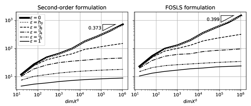
Figure 2. Condition numbers of the preconditioned system for a number of regularization parameters.

6.1.3. Inconsistent data

In case of inconsistent data, there exists no state that exactly explains the data, and $e_{\rm cons}(u_{0})>0$. In this case, it does not make sense to approximate $u_{0}$ within a tolerance that is significantly smaller than $e_{\rm cons}(u_{0})$. Considering for the second order formulation the a priori estimate

$$\|u_{0}-u^{\delta,\delta}_{\varepsilon}\|_{X_{\eta}}\lesssim e_{\rm cons}(u_{0})+e^{\delta}_{\rm approx}(u_{0})+\varepsilon\|\gamma_{0}u_{0}\|_{L_{2}(\Omega)}$$

from Theorem 3.9 and taking the fact into account that choosing $\varepsilon$ small has an only moderate effect on the conditioning of the preconditioned linear system, in the following we take $\varepsilon$ of the order of the best possible approximation error that can be expected, so that $\varepsilon\|\gamma_{0}u_{0}\|_{L_{2}(\Omega)}\lesssim e^{\delta}_{\rm approx}(u_{0})$. Then ideally we would like to stop refining our mesh as soon as $e^{\delta}_{\rm approx}(u_{0})\approx e_{\rm cons}(u_{0})$. In order to achieve this we use the a posteriori error estimator. From Corollary 3.14 we know that

$$e_{\rm cons}(u_{0})\lesssim\sqrt{G_{0}^{\delta}(u^{\delta,\delta}_{\varepsilon})}+e^{\delta}_{\rm osc}(g),$$

where, following the reasoning from the proof of Proposition 3.4,

$$\sqrt{G_{0}^{\delta}(u^{\delta,\delta}_{\varepsilon})} \leq\sqrt{G_{\varepsilon}^{\delta}(u^{\delta,\delta}_{\varepsilon})}\leq\sqrt{G_{\varepsilon}^{\delta}(P_{X^{\delta}}u_{0})}\leq\sqrt{G_{\varepsilon}(P_{X^{\delta}}u_{0})}$$

$$\lesssim e^{\delta}_{\rm approx}(u_{0})+e_{\rm cons}(u_{0})+\varepsilon\|\gamma_{0}u\|_{L_{2}(\Omega)}.$$

We selected $(Y^{\delta})_{\delta\in\Delta}$ such that, in any case for sufficiently smooth $g$, the order of $e^{\delta}_{\rm osc}(g)$ is equal or higher than the generally best possible order of the approximation error, so that $e^{\delta}_{\rm osc}(g)\lesssim e^{\delta}_{\rm approx}(u_{0})$. In view of our earlier assumption on $\varepsilon$, we conclude that

$$e_{\rm cons}(u_{0})\lesssim\sqrt{G_{0}^{\delta}(u^{\delta,\delta}_{\varepsilon})}\lesssim e_{\rm cons}(u_{0})+e^{\delta}_{\rm approx}(u_{0}).$$

Exploiting a common uniform or adaptive refinement strategy, it can be expected that $e^{\delta}_{\rm approx}(u_{0})$ decays with a certain algebraic rate $\rho<1$. Unless $e_{\rm cons}(u_{0})$ is very large, it can therefore be expected that in the early stage of the iteration the a posteriori error estimator $\sqrt{G_{0}^{\delta}(u^{\delta,\delta}_{\varepsilon})}$ decays with this rate, whose value therefore can be monitored. By contrast, as soon as $e^{\delta}_{\rm approx}(u_{0})$ has been reduced to $Ce_{\rm cons}(u_{0})$ for some constant $C>0$, the reduction of $\sqrt{G_{0}^{\delta}(u^{\delta,\delta}_{\varepsilon})}$ in the next step cannot be expected to be better than $\frac{1+C\rho}{1+C}$. Taking $C=1/3$, our strategy will therefore be to stop the iteration as soon as the observed reduction of $\sqrt{G_{0}^{\delta}(u^{\delta,\delta}_{\varepsilon})}$ is worse than $\frac{1+C\rho}{1+C}$.

We have implemented this strategy, and a similar one for the FOSLS formulation, where we apply the discrete spaces as in (6.1), take $\varepsilon=h_{\delta}$, and again consider the unit interval problem (6.2) but now perturb the measured state $f=u|_{I\times\omega}$ by adding $\lambda\mathbb{1}$ to it for various values of $\lambda$.

From the results in Figure 3 we see that the error estimators decrease at first, but then stagnate in the aforementioned sense, at which point we exit the refinement loop (indicated by a $\times$-sign). Further refinement (indicated by the thin dashed lines) is not very useful, and the error estimators stabilize to a value just below $\lambda|\omega|^{1/2}$, being the $L_{2}(I\times\Omega)$-norm of the perturbation we added to the consistent $f$. Knowing that the error estimator converges to $e_{\rm cons}(u_{0})$ (see Remark 3.10), we conclude that $(0,\mathbb{1})\in Y^{\prime}\times L_{2}(I\times\omega)$ is close to being orthogonal to $\operatorname{ran}B_{\omega}$. We note that selecting $\ell=L=2$ produces very similar results.

Figure 3. A posteriori error estimators for the unit interval problem with inconsistent data of varying amounts.

6.2. Unit square

We choose $\Omega:=(0,1)^{2}$. We again subdivide $I$ into $1/h_{\delta}\in\mathbb{N}$ equal subintervals yielding $\mathcal{I}^{\delta}$, and $\Omega$ first into $1/h_{\delta}\times 1/h_{\delta}$ squares and then into $2/h_{\delta}^{2}$ triangles by connecting the lower left and the upper right corner in each square yielding ${\mathcal{T}}^{\delta}$. For a polynomial degree $q$, we take $\varepsilon=h_{\delta}^{q}$. Following the discussion in Sect. 6.1.1, we select $\ell=L=0$ and take our discrete spaces as

$$X^{\delta}_{q}:=\mathcal{S}^{0,q}_{\mathcal{I}^{\delta}}\otimes\mathcal{S}^{0,q}_{{\mathcal{T}}^{\delta},0},~{}~{}Y^{\delta}_{q}:=\mathcal{S}^{-1,q}_{\mathcal{I}^{\delta}}\otimes\mathcal{S}^{0,q}_{{\mathcal{T}}^{\delta},0},~{}~{}\bar{Y}^{\delta}_{q}:=\mathcal{S}^{-1,q-1}_{\mathcal{I}^{\delta}}\otimes\mathcal{S}^{0,q}_{{\mathcal{T}}^{\delta},0},~{}~{}Z^{\delta}_{q}:=\mathcal{S}^{-1,q-1}_{\mathcal{I}^{\delta}}\otimes\mathcal{Z}^{q}_{{\mathcal{T}}^{\delta}}$$

where $\mathcal{Z}^{q}_{{\mathcal{T}}^{\delta}}$ is the BDM space of index $\min(1,q-1)$. Note that the degree $q-1$ in the temporal direction of $\bar{Y}_{q}^{\delta}$ guarantees an oscillation error of the same order as the approximation error, cf. Footnote 7.

We define the preconditioners $\bm{K}^{\delta}_{Y}$, $\bm{K}^{\delta}_{Z}$, and $\bm{K}^{\delta}_{X}$ similar as in the 1D case.

6.2.1. Consistent data

We start with $\omega:=[\tfrac{1}{4},\tfrac{3}{4}]^{2}$ with the prescribed solution $u(t,x,y):=(t^{3}+1)\sin(\pi x)\sin(\pi y)$ and consistent data $(g,f)$. Figure 4 shows for both formulations and $q\in\{1,2\}$ the error estimators as a function of $\dim X^{\delta}\eqsim h_{\delta}^{-3}$. The choice of preconditioners allows to reach the desired tolerance $\langle{\bf r},{\bf K}_{X}^{\delta}{\bf r}\rangle\leq\varepsilon^{2}G_{0}^{\delta}(\tilde{u}_{\varepsilon}^{\delta,\delta})=5.937\cdot 10^{-13}$ for a system with $268\,434\,945$ unknowns in only 96 iterations. The two formulations again exhibit similar performance, and the observed rate $q/3$ is the best possible, in line with Theorem 5.9. Moreover, we see that while theory is incomplete for the second order formulation in practice it works well also for piecewise quadratics.

Figure 4. A posteriori error estimators for the consistent unit square problem with $\omega:=[\tfrac{1}{4},\tfrac{3}{4}]^{2}$ using piecewise linears and quadratics.

Thanks to $X_{\eta}\hookrightarrow C([\eta,1],L_{2}(\Omega))$, the time-slice errors $\|e_{\varepsilon}^{\delta}(t)\|_{L_{2}(\Omega)}$ or $\|\bar{e}_{\varepsilon}^{\delta}(t)\|_{L_{2}(\Omega)}$ are bounded by multiples of $\|e_{\varepsilon}^{\delta}\|_{X_{\eta}}$ or $\|\bar{e}_{\varepsilon}^{\delta}\|_{X_{\eta}}$, respectively. Figure 5 shows these time-slice errors for both formulations using piecewise linears, i.e., $q=1$. We see that for both formulations, the time-slice errors converge with the better rate $2/3$, and that these errors deteriorate for $t\searrow 0$.

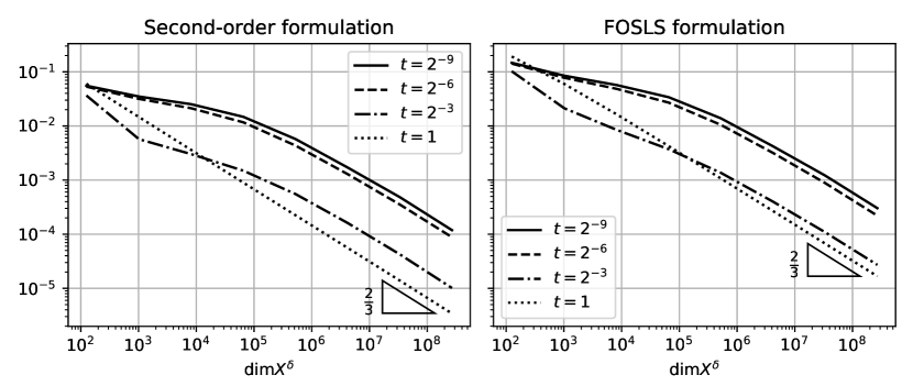
Figure 5. Time-slice errors for the consistent unit square problem with $\omega:=[\tfrac{1}{4},\tfrac{3}{4}]^{2}$ using piecewise linears.

This deterioration becomes much stronger when $\operatorname{diam}\omega\to 0$: taking for example $\omega:=[\tfrac{7}{16},\tfrac{9}{16}]^{2}$, Figure 6 shows that while the error estimators remain nearly unchanged, the time-slice errors fan-out an order of magnitude more than in the case of $\omega:=[\tfrac{1}{4},\tfrac{3}{4}]^{2}$.

Figure 6. Second order formulation for the consistent unit square problem with $\omega:=[\tfrac{7}{16},\tfrac{9}{16}]^{2}$. Left: error estimators; right: time-slice errors.

6.2.2. Inconsistent data

Finally, we return to the case of inconsistent observational data. Again taking $u(t,x,y):=(t^{3}+1)\sin(\pi x)\sin(\pi y)$ and $\omega:=[\tfrac{1}{4},\tfrac{3}{4}]^{2}$, we select consistent forcing data $g:=Bu$ but perturbed observational data $f:=u|_{I\times\omega}+\lambda\mathbb{1}$. Running the strategy outlined in Sect. 6.1.3 with $C=1/3$, with uniform refinements and choosing $\varepsilon=h_{\delta}$, yields the results of Figure 7. We see a situation very similar to the unit interval case: the error estimators decrease at first and then stagnate, at which point we exit the refinement loop. Error estimators again stabilize at around $\lambda|\omega|^{1/2}$.

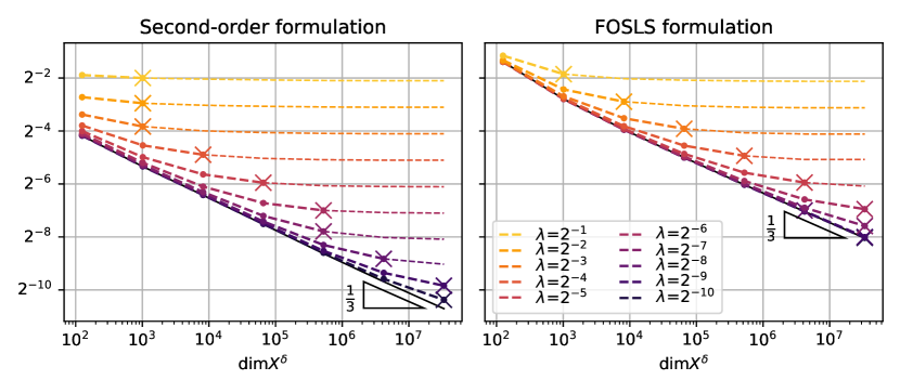
Figure 7. A posteriori error estimators for the unit square problem with inconsistent data of varying amounts.

7. Concluding Remarks

We have seen that basing data assimilation for parabolic problems on infinite-dimensional stable time-space formulations and related regularized least squares functionals has a number of conceptual advantages: one obtains improved a priori error estimates as well as a posteriori error bounds. Among other things the latter ones are important for determining suitable stopping criteria for iterative solvers. Moreover, the design of corresponding preconditioners is based on the infinite-dimensional variational formulation. We have shown that for each fixed regularization parameter $\varepsilon$ the preconditioner is optimal relative to the condition of the regularized problem so that the numerical complexity remains under control. Moreover, the regularization parameter is disentangled from the discretizations which offers possibilities of optimizing its choice.

Furthermore, it will be interesting to relate the present results to the recent state estimation concepts in [BCD⁺11, CDD⁺20, MPPY15] providing error bounds in the full energy norm $\|\cdot\|_{X}$ at the expense of certain stability factors reflecting a geometric relation between $X$ and a certain space of functionals providing the data which, in turn, quantifies the “visibility” of the true states by the sensors. A further important issue is to explore the use of the obtained “static” methods for “dynamic data assimilation”. In this context the underlying stable variational formulations are expected to be crucial for the use of certified reduced models.

A price for building on the above “natural” variational formulations – in the sense that no excess regularity is implied – is to properly discretize dual norms. As pointed out earlier in Remark 4.5, this is avoided in [FK21] by replacing the term $\|C(w,\vec{q})-\tilde{g}\|_{Y^{\prime}}^{2}$ in $H_{\varepsilon}(w;\vec{q})$ (for $K=\mathrm{Id}$) by the $L_{2}$-residual $\|C(w,\vec{q})-\tilde{g}\|_{L_{2}(I;L_{2}(\Omega))}^{2}$. Being reduced to using then a somewhat weaker version of the Carleman estimate, we would obtain a statement similar to that in Corollary 4.4, but with an approximation error $\bar{e}_{{\rm approx}}^{\delta}{(u)}$ measured in a somewhat stronger norm

$$\min_{\{(w,\vec{q})\in X^{\delta}\times Z^{\delta}\colon\partial_{t}w-\operatorname{div}_{\bf x}\vec{q}\in L_{2}(I;L_{2}(\Omega))\}}\|u-w\|_{X}+\|\nabla_{\bf x}u-\vec{q}\|_{Z}$$

$$\qquad\qquad\qquad\qquad\qquad\qquad\qquad\qquad+\|\partial_{t}u-\triangle u-(\partial_{t}w-\operatorname{div}_{\bf x}\vec{q})\|_{L_{2}(I;L_{2}(\Omega))}.$$

Finally, optimal preconditioning in the space $\{(w,\vec{q})\in X^{\delta}\times Z^{\delta}\colon\partial_{t}w-\operatorname{div}_{\bf x}\vec{q}\in L_{2}(I;L_{2}(\Omega))\}$ equipped with the graph norm, seems to be a challenge.

On the other hand, we also have the standard, second order formulation whose implementation is cheaper, and at least in the above experiments performs well also in cases beyond the regime so far covered by theory.

Appendix A Construction of the biorthogonal projector as in Remark 5.3 for $d=q=2$ and one red-refinement

A basis for ${\mathcal{S}}_{{\mathcal{T}}^{\delta},0}^{0,2}+{\mathcal{S}}_{{\mathcal{T}}^{\delta}}^{-1,1}$ is given by the sum of the union over $T^{\prime}\in{\mathcal{T}}^{\delta}$ of the usual nodal basis for $P_{1}(T^{\prime})$, and the union over the internal edges of ${\mathcal{T}}^{\delta}$ of the continuous piecewise quadratic bubble associated to that edge, whose support extends to the two neighbouring triangles in ${\mathcal{T}}^{\delta}$. Indeed, one easily verifies that this set of functions is linearly independent, and that each function from either ${\mathcal{S}}_{{\mathcal{T}}^{\delta},0}^{0,2}$ or ${\mathcal{S}}_{{\mathcal{T}}^{\delta}}^{-1,1}$ is in its span.

We consider the restriction of this basis to one $T^{\prime}\in{\mathcal{T}}^{\delta}$, and subsequently transfer it into a collection of functions on a ‘reference triangle’ $\hat{T}$ with $|\hat{T}|=1$ by an affine transformation. We denote the resulting functions as indicated in Figure 8.

Figure 8. Notation of the basis functions at the ‘primal side’ with the indices of the missing basis functions obtained by permuting the barycentric coordinates.

At the ‘dual side’, we consider the nodal basis of the continuous piecewise quadratics w.r.t. the red-refinement of $\hat{T}$, where we omit the basis functions associated to the vertices of $\hat{T}$. We denote these basis functions as indicated in Figure 9.

Figure 9. Notation at the ‘dual side’.

We now apply the following transformations:

1. On the primal side, we redefine

   $$e_{\frac{1}{2},\frac{1}{2},0}\leftarrow e_{\frac{1}{2},\frac{1}{2},0}-{\textstyle\frac{7}{10}}(v_{1,0,0}+v_{0,1,0})+{\textstyle\frac{7}{30}}v_{0,0,1},$$

   and update $e_{\frac{1}{2},0\frac{1}{2}}$ and $e_{0,\frac{1}{2},\frac{1}{2}}$ analogously. As a consequence, we obtain $\operatorname{span}\{e_{\frac{1}{2},\frac{1}{2},0},e_{\frac{1}{2},0,\frac{1}{2}},e_{0,\frac{1}{2},\frac{1}{2}}\}\perp\operatorname{span}\{\tilde{v}_{1,0,0},\tilde{v}_{0,1,0},\tilde{v}_{0,0,1}\}$.

2. On the dual side, we redefine

   $$\tilde{e}_{\frac{1}{2},\frac{1}{2},0}\leftarrow{\textstyle\frac{1}{102}}\tilde{e}_{\frac{1}{2},\frac{1}{2},0}-{\textstyle\frac{7}{2312}}(\tilde{e}_{\frac{3}{4},\frac{1}{4},0}+\tilde{e}_{\frac{1}{4},\frac{3}{4},0}),$$

   and update $\tilde{e}_{\frac{1}{2},0\frac{1}{2}}$ and $\tilde{e}_{0,\frac{1}{2},\frac{1}{2}}$ analogously. Consequently, $\{e_{\frac{1}{2},\frac{1}{2},0},e_{\frac{1}{2},0,\frac{1}{2}},e_{0,\frac{1}{2},\frac{1}{2}}\}$ and $\{\tilde{e}_{\frac{1}{2},\frac{1}{2},0},\tilde{e}_{\frac{1}{2},0,\frac{1}{2}},\tilde{e}_{0,\frac{1}{2},\frac{1}{2}}\}$ became biorthogonal. The functions $e_{\pi(\frac{3}{4},\frac{1}{4},0)}$ for any permutation $\pi$, will not play any role anymore, and will be ignored.

3. On the dual side, we redefine

   $$\left[\begin{array}[]{@{}c@{}}\tilde{v}_{1,0,0}\\ \tilde{v}_{0,1,0}\\ \tilde{v}_{0,0,1}\end{array}\right]\leftarrow 12\left[\begin{array}[]{@{}rrr@{}}3&-1&-1\\ -1&3&-1\\ -1&-1&3\\ \end{array}\right]\left[\begin{array}[]{@{}c@{}}\tilde{v}_{1,0,0}\\ \tilde{v}_{0,1,0}\\ \tilde{v}_{0,0,1}\end{array}\right].$$

   Consequently, $\{v_{1,0,0},v_{0,1,0},v_{0,0,1}\}$ and $\{\tilde{v}_{1,0,0},\tilde{v}_{0,1,0},\tilde{v}_{0,0,1}\}$ became biorthogonal.

After these 3 steps, the $6\times 6$ ‘local generalized mass matrix’ that contains the $L_{2}(\hat{T})$-inner products between all primal functions, grouped into $v$- and $e$-functions, and all (remaining) dual functions, grouped into $\tilde{v}$- and $\tilde{e}$-functions, has the $2\times 2$ block structure $\left[\begin{array}[]{@{}cc@{}}\mathrm{Id}&\tfrac{9}{32}\mathrm{Id}-\tfrac{31}{32}\mathbb{1}\\ 0&\mathrm{Id}\end{array}\right]$, with $\mathbb{1}$ the $3\times 3$ all-ones matrix (and with the $\tilde{e}$-functions ordered as the ‘opposite’ $v$-functions). The invertibility of this matrix confirms that both collections of 6 primal and 6 dual functions are linearly independent.

We use these primal and dual functions on the reference triangle $\hat{T}$ to construct collections of primal and dual functions on $\Omega$ by the usual lifting by means of an affine bijection between $\hat{T}$ and any $T^{\prime}\in{\mathcal{T}}^{\delta}$. When doing so, we connect the functions of $e$ or $\tilde{e}$-type continuously over ‘their’ edges, and omit them on edges on $\partial\Omega$.

Each function of $v$ or $\tilde{v}$-type is supported on one $T^{\prime}\in{\mathcal{T}}^{\delta}$, and we multiply them by the factor $|T^{\prime}|^{-\frac{1}{2}}$. The functions of $e$ or $\tilde{e}$-type are supported on two adjacent $T^{\prime},T^{\prime\prime}\in{\mathcal{T}}^{\delta}$, and we multiply them by the factor $(|T^{\prime}|+|T^{\prime\prime}|)^{-\frac{1}{2}}$.

By their construction, the resulting primal and dual collections, denoted by $\Phi^{\delta}$ and $\tilde{\Phi}^{\delta}$, are uniformly $L_{2}(\Omega)$-Riesz systems, with mass matrices whose extremal eigenvalues are inside the interval spanned by the extremal eigenvalues of the corresponding primal or dual mass matrices on the reference triangle.

Furthermore, $\operatorname{span}\Phi^{\delta}={\mathcal{S}}_{{\mathcal{T}}^{\delta},0}^{0,2}+{\mathcal{S}}_{{\mathcal{T}}^{\delta}}^{-1,1}$, and $\operatorname{span}\tilde{\Phi}^{\delta}\subset{\mathcal{S}}_{{\mathcal{T}}_{S}^{\delta},0}^{0,2}$, with ${\mathcal{T}}_{S}^{\delta}$ being constructed from ${\mathcal{T}}^{\delta}$ by one uniform red-refinement.

The generalized mass matrix, i.e., the matrix with the $L_{2}(\Omega)$-inner products between all primal functions, grouped into $v$- and $e$-functions, and all dual functions, grouped into $\tilde{v}$- and $\tilde{e}$-functions, has the $2\times 2$ block structure $\left[\begin{array}[]{@{}cc@{}}\mathrm{Id}&*\\ 0&\mathrm{Id}\end{array}\right]$. The uniform $L_{2}(\Omega)$-Riesz basis property of both $\Phi^{\delta}$ and $\tilde{\Phi}^{\delta}$ shows that the spectral norm of the non-zero off-diagonal block is uniformly bounded. By now redefining $\Phi^{\delta}\leftarrow\left[\begin{array}[]{@{}cc@{}}\mathrm{Id}&-*\\ 0&\mathrm{Id}\end{array}\right]\Phi^{\delta}$, we obtain primal and dual uniformly $L_{2}(\Omega)$-Riesz systems that are biorthogonal, where $\operatorname{span}\Phi^{\delta}={\mathcal{S}}_{{\mathcal{T}}^{\delta},0}^{0,2}+{\mathcal{S}}_{{\mathcal{T}}^{\delta}}^{-1,1}$ and $\operatorname{span}\tilde{\Phi}^{\delta}\subset{\mathcal{S}}_{{\mathcal{T}}_{S}^{\delta},0}^{0,2}$.

In view of the supports of the dual functions, and those of the primal functions before the last transformation, we infer that the support of a function in $\tilde{\Phi}^{\delta}$ is contained in either one $T^{\prime}\in{\mathcal{T}}^{\delta}$ ($\tilde{v}$-type), or in the union of two triangles from ${\mathcal{T}}^{\delta}$ that share an edge ($\tilde{e}$-type), and that the support of a function in $\Phi^{\delta}$ is contained in either the union of two triangles from ${\mathcal{T}}^{\delta}$ that share an edge ($e$-type), or in the union of $T^{\prime}\in{\mathcal{T}}^{\delta}$ and those at most three $T^{\prime\prime}\in{\mathcal{T}}^{\delta}$ that share an edge with $T^{\prime}$. We conclude that the biorthogonal projector $P_{2}^{\delta}\colon u\mapsto\langle u,\Phi^{\delta}\rangle_{L_{2}(\Omega)}\tilde{\Phi}^{\delta}$ satisfies both conditions (5.4) and (5.6).

References

• [AK01] O. Axelsson and I. Kaporin. Error norm estimation and stopping criteria in preconditioned conjugate gradient iterations. Numer. Linear Algebra Appl., 8(4):265–286, 2001.
• [And13] R. Andreev. Stability of sparse space-time finite element discretizations of linear parabolic evolution equations. IMA J. Numer. Anal., 33(1):242–260, 2013.
• [And16] R. Andreev. Wavelet-in-time multigrid-in-space preconditioning of parabolic evolution equations. SIAM J. Sci. Comput., 38(1):A216–A242, 2016.
• [Ash15] A. C. L. Ashton. Elliptic PDEs with constant coefficients on convex polyhedra via the unified method. J. Math. Anal. Appl., 425(1):160–177, 2015.
• [BBLD15] E. Bécache, L. Bourgeois, L. Franceschini, and J. Dardé. Application of mixed formulations of quasi-reversibility to solve ill-posed problems for heat and wave equations: the 1D case. Inverse Probl. Imaging, 9(4):971–1002, 2015.
• [BCD+11] P. Binev, A. Cohen, W. Dahmen, R. DeVore, G. Petrova, and P. Wojtaszczyk. Convergence rates for greedy algorithms in reduced basis methods. SIAM J. Math. Anal., 43(3):1457–1472, 2011.
• [BFMO21] E. Burman, A. Feizmohammadi, A. Münch, and L. Oksanen. Space time stabilized finite element methods for a unique continuation problem subject to the wave equation. ESAIM Math. Model. Numer. Anal. 55:S969–S991, 2021.
• [BIHO18] E. Burman, J. Ish-Horowicz, and L. Oksanen. Fully discrete finite element data assimilation method for the heat equation. ESAIM Math. Model. Numer. Anal., 52(5):2065–2082, 2018.
• [BLO18] E. Burman, M. G. Larson, and L. Oksanen. Primal- dual mixed finite element methods for the elliptic Cauchy problem. SIAM J. Numer. Anal. 56(6): 3480–3509, 2018.
• [BO18] E. Burman and L. Oksanen. Data assimilation for the heat equation using stabilized finite element methods. Numer. Math., 139(3):505–528, 2018.
• [BR18] L. Bourgeois, and A. Recoquillay. A mixed formulation of the Tikhonov regularization and its application to inverse PDE problems. ESAIM Math. Model. Numer. Anal. 52(1):123–145, 2018.
• [BY14] R.E. Bank and H. Yserentant. On the $H^{1}$-stability of the $L_{2}$-projection onto finite element spaces. Numer. Math., 126(2):361–381, 2014.
• [CDD+20] A. Cohen, W. Dahmen, R. DeVore, J. Fadili, O. Mula, and J. Nichols. Optimal reduced model algorithms for data-based state estimation. SIAM J. Numer. Anal., 58(6):3355–3381, 2020.
• [CDG14] C. Carstensen, L. Demkowicz, and J. Gopalakrishnan. A posteriori error control for DPG methods. SIAM J. Numer. Anal., 52(3):1335–1353, 2014.
• [CDW12] A. Cohen, W. Dahmen, and G. Welper. Adaptivity and variational stabilization for convection-diffusion equations. ESAIM Math. Model. Numer. Anal., 46:1247–1273, 2012.
• [Che14] L. Chen. A simple construction of a Fortin operator for the two dimensional Taylor-Hood element. Comput. Math. Appl., 68(10):1368–1373, 2014.
• [Dal94] R. Daley. Atmospheric Data Analysis. Cambridge Atmospheric and Space Science Series. Cambridge University Press, Cambridge, UK, 1994.
• [DHH13] J. Dardé, A. Hannukainen, and N. Hyvönen. An Hdiv-based mixed quasi-reversibility method for solving elliptic Cauchy problems. SIAM J. Numer. Anal. 51(4):2123–2148, 2013.
• [DL92] R. Dautray and J.-L. Lions. Mathematical analysis and numerical methods for science and technology. Vol. 5. Springer-Verlag, Berlin, 1992. Evolution problems I.
• [FK21] T. Führer and M. Karkulik. Space-time least-squares finite elements for parabolic equations. Comput. Math. Appl. 92:27–36, 2021.
• [GM97] G. H. Golub and G. Meurant. Matrices, moments and quadrature. II. How to compute the norm of the error in iterative methods. BIT, 37(3):687–705, 1997.
• [GS21] G. Gantner and R.P. Stevenson. Further results on a space-time FOSLS formulation of parabolic PDEs. ESAIM Math. Model. Numer. Anal. 55(1):283–299, 2021.
• [LLD06] J.M. Lewis, S. Lakshmivarahan, and S. Dhall. Dynamic Data Assimilation. Encyclopedia of Mathematics and its Applications. Cambridge University Press, Cambridge, UK, 2006.
• [Maj16] A.J. Majda. Introduction to turbulent dynamical systems in complex systems, volume 5 of Frontiers in Applied Dynamical Systems: Reviews and Tutorials. Springer, 2016.
• [MPPY15] Y. Maday, A.T. Patera, J.D. Penn, and M. Yano. A parameterized-background data-weak approach to variational data assimilation: formulation, analysis, and application to acoustics. Int. J. Numer. Methods Eng., 102(5):933–965, 2015.
• [MS17] A. Münch, and D.A. Souza. Inverse problems for linear parabolic equations using mixed formulations - Part 1: Theoretical analysis. J. Inverse Ill-Posed Probl. 25(4):445–468, 2017,
• [MT13] G. Meurant and P. Tichý. On computing quadrature-based bounds for the $A$-norm of the error in conjugate gradients. Numer. Algorithms, 62(2):163–191, 2013.
• [RS18] N. Rekatsinas and R. Stevenson. An optimal adaptive wavelet method for first order system least squares. Numer. Math., 140(1):191–237, 2018.
• [Sch97] J. Schöberl. NETGEN an advancing front 2d/3d-mesh generator based on abstract rules. Comput. Vis. Sci, 1(1), 1997.
• [Sch14] J. Schöberl. C++11 implementation of finite elements in ngsolve. Technical report, Institute for Analysis and Scientific Computing. Vienna University of Technology, 2014.
• [SS09] Ch. Schwab and R.P. Stevenson. A space-time adaptive wavelet method for parabolic evolution problems. Math. Comp., 78:1293–1318, 2009.
• [SvVW21] R.P. Stevenson, R. van Venetië, and J. Westerdiep. A wavelet-in-time, finite element-in-space adaptive method for parabolic evolution equations. 2021, arXiv:2101.03956.
• [SW20] R.P. Stevenson and J. Westerdiep. Stability of Galerkin discretizations of a mixed space-time variational formulation of parabolic evolution equations. IMA J. Numer. Anal., 2020.
• [SW21] R. Stevenson and J. Westerdiep. Minimal residual space-time discretizations of parabolic equations: Asymmetric spatial operators. 2021, arXiv:2106.01090.
• [Wlo82] J. Wloka. Partielle Differentialgleichungen. B. G. Teubner, Stuttgart, 1982. Sobolevräume und Randwertaufgaben.