Variable stars in the VVV globular clusters.

Abstract

Context. The Galactic globular clusters (GGCs) located in the inner regions of the Milky Way suffer from high extinction that makes their observation challenging. High densities of field stars in their surroundings complicate their study even more. The VISTA Variables in the Via Lactea (VVV) survey provides a way to explore these GGCs in the near-infrared where extinction effects are highly diminished.

Aims. We conduct a search for variable stars in several inner GGCs, taking advantage of the unique multi-epoch, wide-field, near-infrared photometry provided by the VVV survey. We are especially interested in detecting classical pulsators that will help us constrain the physical parameters of these GGCs. In this paper, the second of a series, we focus on NGC 6656 (M 22), NGC 6626 (M 28), NGC 6569, and NGC 6441; these four massive GGCs have known variable sources, but quite different metallicities. We also revisit 2MASS-GC 02 and Terzan 10, the two GGCs studied in the first paper of this series.

Methods. We present an improved method and a new parameter that efficiently identify variable candidates in the GGCs. We also use the proper motions of those detected variable candidates and their positions in the sky and in the color-magnitude diagrams to assign membership to the GGCs.

Results. We identify and parametrize in the near-infrared numerous variable sources in the studied GGCs, cataloging tens of previously undetected variable stars. We recover many known classical pulsators in these clusters, including the vast majority of their fundamental mode RR Lyrae. We use these pulsators to obtain distances and extinctions toward these objects. Recalibrated period-luminosity-metallicity relations for the RR Lyrae bring the distances to these GGCs to a closer agreement with those reported by Gaia, except for NGC 6441, which is an uncommon Oosterhoff III GGC. Recovered proper motions for these GGCs also agree with those reported by Gaia, except for 2MASS-GC 02, the most reddened GGC in our sample, where the VVV near-infrared measurements provide a more accurate determination of its proper motions.

1 Introduction

Many Galactic globular clusters (GGCs) located in the inner regions of the Milky Way (within 3 kpc from the Galactic center) still lack a proper determination of their physical parameters. The analysis of the color-magnitude diagrams (CMDs), which is the most common tool to extract this information, is severely hampered when applied to these objects. We need to add two specific issues more common in the inner parts of the Galaxy to the usual problems we face when studying the globular clusters of the outer Galaxy (e.g., high crowding, saturation by bright stars). The first issue is the presence of high extinction and reddening, which usually change differentially over the field of view of these GGCs. The second issue is the high density of field stars that appear in the CMDs superimposed with the stellar population of these GGCs, making it difficult to disentangle the field from the cluster especially in the most poorly populated GGCs.

To diminish the effects of extinction, observations of these GGCs can be carried out in the near-infrared. Extinction at these wavelengths is significantly smaller than in the optical ($\mathcal{A}_{K}\sim 0.1\mathcal{A}_{V}$; see Table 2 in Catelan et al. 2011). To take full advantage of this fact, the VISTA Variables in the Via Lactea (VVV) survey (Minniti et al., 2010; Saito et al., 2012) observed the inner regions of the Galaxy in the near-infrared in recent years. VVV is a European Southern Observatory (ESO) public survey that was conducted between 2010 and 2016, covering 560 sq. degrees of the Galactic bulge and an adjacent region of the inner disk. Observations in five near-infrared filters $ZYJHK_{s}$ were performed, and observations in $K_{s}$ of the whole region were taken in multiple epochs, aiming to explore the presence of variable stars and other variable phenomena in this area of the sky.

There are 36 GGCs in the area covered by the VVV survey, according to the 2010 version of the Harris (1996) catalog (from now on the Harris catalog), along with tens of new candidates (e.g., Minniti et al. 2017; Camargo & Minniti 2019; Minniti et al. 2019; Gran et al. 2019; Palma et al. 2019; for a recent update, see Bica et al. 2019). In a series of papers, we are exploring the variable stars present in these GGCs, aiming to better characterize the cluster in which they reside. Among them, RR Lyrae stars are fundamental for our purposes. Not only are these stars quite common in (many) globular clusters, but their period-luminosity (PL) relation, especially tight in the near-infrared (Longmore et al., 1986; Catelan et al., 2004), makes them excellent standard candles that allow us to accurately infer their distances and extinctions; we showed this for 2MASS-GC 02 and Terzan 10 in Alonso-García et al. (2015), which we refer to from now on as Paper I. The GGCs are clumped into two main groups (Oosterhoff, 1939; Catelan, 2009; Smith et al., 2011), according to the characteristics of the fundamental-mode RR Lyrae (RRab) that they contain: the Oosterhoff I group shows RRab stars with shorter periods ($\langle P_{\rm ab}\rangle\sim 0.55$ days), while the Oosterhoff II have RRab stars with longer periods ($\langle P_{\rm ab}\rangle\sim 0.64$ days). Between these two groups, there is an almost empty region called the Oosterhoff gap, at $\langle P_{\rm ab}\rangle\sim 0.60\pm 0.02$ days. Oosterhoff II GGCs also tend to be more metal-poor than Oosterhoff I GGCs and to have a higher ratio of first-overtone RR Lyrae (RRc) to RRab stars. A couple of GGCs containing $\langle P_{\rm ab}\rangle$ too long for their high metallicities have been classified as Oosterhoff III GGCs (Pritzl et al., 2000).

Table 1: Positions and physical parameters of the target clusters.

Cluster	$\alpha$(J2000)	$\delta$(J2000)	$l$	$b$	$[{\rm Fe/H}]$	$M_{V}$	c	$r_{t}$
	(h:m:s)	(d:m:s)	(deg)	(deg)	(dex)	(mag)		(arcmin)
NGC 6441	17:50:13	-37:03:04	353.53	-5.01	-0.46	-9.63	1.74	7.14
Terzan 10	18:02:58	-26:04:00	4.42	-1.86	-1.59	-6.35	0.75	5.06
2MASS-GC 02	18:09:37	-20:46:44	9.78	-0.62	-1.08	-4.86	0.95	4.90
NGC 6569	18:13:39	-31:49:35	0.48	-6.68	-0.76	-8.28	1.31	7.15
NGC 6626 (M 28)	18:24:33	-24:52:12	7.80	-5.58	-1.32	-8.16	1.67	11.22
NGC 6656 (M 22)	18:36:24	-23:54:12	9.89	-7.55	-1.70	-8.50	1.38	31.90

In this second paper of the series, we focus on several well-known GGCs located in the VVV footprint: NGC 6441, NGC 6569, NGC 6626 (M 28), and NGC 6656 (M 22). These GGCs show a significant range in their metallicities (see Table 1) and in their Oosterhoff classification. They differ from those studied in Paper I because they lie in regions in which extinction is lower, although still high for outer GGCs standards. These GGCs are also better populated than the GGCs studied in Paper I, and they lie in fields in which the stellar background densities are lower. Finally, they possess recent distance estimations inferred from Gaia data (Baumgardt et al., 2019), and they contain significant numbers of variable stars in their fields present in the most recent version of the Clement et al. (2001) catalog of variable stars in the GGCs (from now on, the Clement catalog) and in the collection of variable stars in the inner Milky Way by Soszyński et al. (2016, 2017, 2019) from the Optical Gravitational Lensing Experiment (OGLE). Therefore, by drawing a comparison with this previous literature, we aim to examine the reliability of our methods to detect variable stars and to infer the physical parameters (distance, extinction, and proper motion [PM]) for their GGCs. While achieving this, we also provide a look at the variable stars of these GGCs from their innermost regions to their outskirts at near-infrared wavelengths for the first time. Additionally, we also revisit 2MASS-GC 02 and Terzan 10, the GGCs from Paper I, to check the advantages and drawbacks of our updated approach to detect variable sources.

The paper is divided into the following sections: In Sect. 2, we describe our database; in Sect. 3 we develop our improved method to detect variable stars; in Sect. 4, 5, and 6 we implement this method firstly on NGC 6656 (M 22), then on NGC 6441, NGC 6569, NGC 6626 (M 28), and finally on 2MASS-GC 02 and Terzan 10, providing a description of the variable star candidates we found in their fields; we also select potential members of each cluster according to their PM and their positions in the CMD, and use these sources to obtain the distances and extinctions toward these GGCs; finally, in Sect. 7 we summarize our conclusions.

2 Observations and datasets

In our analysis, we used observations from VVV (Minniti et al., 2010), one of the six original ESO public surveys conducted with the 4.1m VISTA telescope in the Cerro Paranal Observatory. The camera installed in the telescope provides wide-field images of 1.6 square degrees of the sky, with gaps due to the separation of the 16 chips in the camera. The VVV survey uses five near-infrared filters ($Z$, $Y$, $J$, $H$, and $K_{s}$) and its footprint for the Galactic bulge region is divided into 196 individual fields. The observing strategy for every VVV field, detailed in Saito et al. (2012), consists in taking two consecutive slightly dithered images of the sky in a given filter which, when later on combined into a so-called stacked image, allow the correction of cosmetic defects from the different chips. Along with this pattern, a mosaic of six consecutive pointings is taken for every field and filter to provide a contiguous coverage of the observed field, covering the gaps among the chips in the camera. Every field is observed at least twice in $Z$, $Y$, $J$, and $H$, and at least 70 times in the $K_{s}$ filter. The $K_{s}$ observations in every epoch have a median exposure time of 16 seconds (Saito et al., 2012) and were taken in a nonuniform, space-varying cadence (Dékány et al., 2019).

Our analysis is based on the VVV photometry and astrometry provided by VIRAC2, an updated version of the VVV Infrared Astrometric Catalogue (VIRAC; Smith et al., 2018). A complete description of the new features of VIRAC2 will be given in an upcoming dedicated paper (Smith et al., in prep.). Suffice it to say here that this version of VIRAC uses DoPHOT (Schechter et al., 1993; Alonso-García et al., 2012) to extract the point-spread function photometry from the VVV stacked images, significantly reducing the missing sources and increasing the completeness of the sample, especially in the highly crowded GGCs (Alonso-García et al., 2018). Photometric zero points for each observation were measured by globally minimizing the error-normalized offsets between multiple detections of individual sources and offsets from 2MASS (transformed to the VISTA photometric system as per González-Fernández et al. 2018) where available. A further calibration was applied to remove spatially coherent residual structure and match the photometric uncertainties to residual scatter. This way the calibration offsets reported in Hajdu et al. (2020) are effectively resolved. The VIRAC2 catalog provides us with the VVV mean magnitudes, PMs, and near-infrared light curves for all the detected sources.

3 Variability analysis

We modified the variability analysis presented in Paper I to optimize for its use with VIRAC2 on the detection and proper characterization of classical pulsators. These are the variable stars that we are more interested in detecting because they can be used as standard candles. According to our experience, Cepheids and RRab stars are the classical pulsators that stand out the most in the near-infrared VVV observations. Even though their light curves are more sinusoidal and their amplitudes are smaller in the near-infrared than at optical wavelengths (Angeloni et al., 2014; Catelan & Smith, 2015), the features of their light curves still provide ways to properly identify them within the VVV data, as shown in Paper I. The smaller amplitudes of the RRc stars complicate their identification as variable sources. Even when they are identified as variable stars, their almost sinusoidal light curves make it difficult to conclusively assign them to this class using only their VVV near-infrared photometry. Therefore, the analysis described in this section aims to mainly identify most of the Cepheids and RRab stars with good-quality light curves in the VVV GGCs fields. Some RRc stars and eclipsing binaries are also identified, as shown in the next sections.

The first step in our analysis was to take all sources from VIRAC2 that lie inside the tidal radius of the selected GGCs (see Table 1). After that, we selected stars that were measured in at least half of the $K_{s}$ observations that were taken for their region of sky. That way we disregarded spurious or very low signal-to-noise detections. The next step in our analysis looked at the distribution of the median absolute deviation (MAD) of the $K_{s}$ magnitudes in the different epochs for the stars in a given cluster, as a function of its median $K_{s}$ magnitude. As classical pulsators show variations along all its phased light curve, this produces a higher MAD than for a non-variable source at a given magnitude. For other types of variable stars such as eclipsing binaries with short and/or not well-sampled eclipses, the MAD may not be such a good indicator of variability. We calculated the median and the standard deviation of the MAD as a function of the median $K_{s}$ magnitude. For the next step of our analysis we kept only sources that are more than $1\sigma$ away from the median of the MAD (see Fig. 1). We noticed from some preliminary tests with previously known variables in our sample of GGCs that for stars under this cutoff we were unable to detect classical pulsators with good-quality light curves. By applying this cutoff, we reduced the number of stars to be analyzed to $\sim 10\%$ of the original sample.

Figure 1: MAD vs. median of the $K_{s}$ magnitudes for the different epochs with VVV detections for the stars in M 22, serving as an example of the preliminary selection to detect variable candidates. The green dots show the stars we keep for the next step of the analysis. They are located $1\sigma$ above the median of the distribution, shown by the red line.

We then looked for periodicity in the signal of every source we kept. In order to do that, first we submitted the light curve of the remaining sources to a generalized Lomb-Scargle (GLS) analysis (Zechmeister & Kürster, 2009). We analyzed the interval of frequencies $[0.01-10]$ days^-1, which covers all RR Lyrae and Cepheids. As in Paper I, we eliminated sources with significant gaps in a given section of their folded light curve and aliased sources with values for frequency close to integers of days^-1. Using the best period the GLS algorithm provided, we fitted a Fourier series to the folded light curve. We masked those epochs that departed more than $3\sigma$ from the Fourier fit. We averaged values from the same mosaic sequence (see Sect. 2) for a more accurate sampling of the light curve. Since the time taken to observe these sequences for a given VVV field and filter is much shorter than the period of the variable sources we are measuring, we can consider observations in one of these sequences to have been taken at the same epoch. We then recalculated the period of the variable candidate using the GLS algorithm, and repeated the described sequence iteratively until we reached a convergence in the period. After this, for every source we calculated $\rho$, the ratio of the standard deviation of the distribution of $K_{s}$ mosaic-averaged magnitudes from the different epochs available for that source to the standard deviation from its Fourier fit. The ratio $\rho$ between these two standard deviations provides us with a good approximation to a by-eye identification and quality assignment for variable sources (see Fig. 2). After some visual inspection, we adopted a value of $\rho=1.50$ as our cutoff point for the variable stars in the GGCs reported in this study, except for Terzan 10 in which we used $\rho=1.30$ as our cutoff point owing to the higher number of epochs available for this cluster. A quick visual inspection of the shape of the light curves above this cutoff value allowed us to reject a few false positives, mainly owing to blending from two sources in the same light curve.

Figure 2: VVV $K_{s}$ phase-folded light curves for some variable stars in M 22 in common with the OGLE catalog, as examples of how their quality changes with the $\rho$ parameter defined in the text. From top to bottom, light curves are ordered according to their decreasing $\rho$ value. The upper two panels, with the higher $\rho$ values, represent clear identifications of the variable nature of these stars according to their VVV light curves. The third panel, where $\rho=1.50$, represents a detection just in our cutoff point. In the lower panel, the poor quality of the VVV light curve makes it difficult to separate this true variable source from other false triggers with similar $\rho$ values, rendering their identification as a real variable problematic.

For all the remaining variable candidates, we proceeded to obtain their observational parameters. As in Paper I, the apparent $K_{s}$-band equilibrium brightnesses of the stars $\langle K_{s}\rangle$ were estimated by the intensity-averaged magnitudes of the stars, computed from the Fourier fits to the light curves, and the total amplitudes of the light curves $A_{K_{s}}$ were computed from the Fourier fits as well. We have observations for filters $Z$, $Y$, $J$, and $H$ only in approximately two epochs per filter. To calculate the $\lambda-K_{s}$ apparent colors, we obtained the $K_{s}$ magnitude from the Fourier fit of the $K_{s}$ light curve at the same phase where the measurements for the other filters were taken, and after that, we took the mean of the colors from the few different epochs available for a given filter. Finally, we proceeded to examine the light curves to assign a variable type to the different candidates. As mentioned in Paper I, this eyeball classification is complicated by the fact that the near-infrared $K_{s}$ light curves usually contain fewer outstanding features than in the optical. Although we could reliably classify Cepheids, RRab stars, and some eclipsing binaries, there were a significant number of candidates that we left with their variable type as undecided. For stars in common with the other catalogs and variable types difficult to characterize in the near-infrared (e.g., RRc stars, W UMa-type [EW] eclipsing binaries), we kept the classification from their optical light curves. For stars classified as eclipsing binaries, we doubled the periods reported by our algorithms because they do not separate primary and secondary eclipses in these variable stars.

4 NGC 6656 (M 22)

NGC 6656 (M 22) is the most metal-poor cluster from the sample of VVV GGCs we are considering in this paper. Its high brightness and moderate concentration when compared with other VVV GGCs (see Table 1 for its physical characteristics), along with its relative proximity, makes NGC 6656 the GGC that subtends the largest sky area in the original VVV footprint, rivaled only by FSR 1758 (Barbá et al., 2019), observed by the VVV eXtended survey (VVVX; Minniti, 2018).

4.1 Variables in the cluster area

There have been a significant number of studies looking for variables in this Oosterhoff II GGC, dating back to those by Bailey (1902), Shapley (1927), and Sawyer (1944), up to the most recent works by Kunder et al. (2013) and Rozyczka et al. (2017). Ours is the first study in the near-infrared that covers the whole cluster, from its very center out to its tidal radius. Following the steps described in Sect. 3, we identified 439 variable candidates in the field of this GGC. We present their physical properties in Table 2. There are 142 variable sources reported in the Clement catalog for M 22, while we found 604 variable stars in the OGLE catalog inside the tidal radius of M 22 and there are 360 variable sources in the catalog presented by Rozyczka et al. (2017). As shown in the comparison in Table 2, most variable stars in our catalog are also present in these other catalogs, but there are 155 variable candidates that were not previously reported.

Table 2: Properties of the variable candidates in NGC 6656 (M 22).

ID	$ID_{Clement}$	$ID_{OGLE}$	$ID_{Ros17}$	$\alpha$ (J2000)	${\delta}$ (J2000)	Distance	Period	$A_{K_{s}}$	$\langle K_{s}\rangle$	$Z-K_{s}$	$Y-K_{s}$	$J-K_{s}$	$H-K_{s}$	$\mu_{\alpha^{\ast}}$	$\mu_{\delta}$	Member	Type
		(OGLE-BLG-)		(h:m:s)	(d:m:s)	(arcmin)	(days)	(mag)	(mag)	(mag)	(mag)	(mag)	(mag)	(mas/yr)	(mas/yr)
C1	KT-55	–	KT-55	18:36:23.25	-23:53:58.1	0.29	0.658743	0.255	12.047	0.699	0.538	0.386	0.085	9.322	-5.336	Yes	RRab
C2	V24	T2CEP-0927	24	18:36:21.80	-23:54:13.4	0.5	1.714805	0.284	11.104	0.988	0.774	–	0.75	10.54	-4.359	Yes	Cep
C3	V23	RRLYR-36672	23	18:36:23.04	-23:54:41.7	0.54	0.551593	0.307	12.253	0.911	0.704	0.412	0.104	10.056	-5.662	Yes	RRab
C4	V1	RRLYR-36670	1	18:36:19.57	-23:54:33.0	1.07	0.615536	0.309	12.12	0.883	0.669	0.495	0.115	8.909	-5.574	Yes	RRab
C5	–	–	–	18:36:25.20	-23:53:04.8	1.15	0.105017	0.311	15.689	–	0.382	0.236	0.028	16.141	1.402	Yes	?
C6	V21	RRLYR-36675	21	18:36:25.76	-23:52:58.2	1.29	0.327135	0.08	12.441	0.622	0.448	0.368	0.096	9.948	-5.237	Yes	RRc
C7	V4	RRLYR-36673	4	18:36:23.37	-23:55:29.4	1.3	0.716398	0.28	11.959	0.913	0.695	0.498	0.115	10.284	-6.561	Yes	RRab
C8	V12	RRLYR-36674	12	18:36:23.77	-23:55:39.1	1.45	0.322624	0.099	12.451	0.682	0.492	0.335	0.069	10.372	-5.292	Yes	RRc
C9	KT-14	–	KT-14	18:36:30.69	-23:53:54.1	1.56	0.373642	0.081	12.291	0.735	0.534	0.355	0.091	10.267	-7.793	Yes	RRc
C10	KT-12	RRLYR-36679	KT-12	18:36:30.94	-23:53:49.1	1.63	0.443619	0.222	14.572	0.731	0.567	0.496	0.17	-4.454	-3.644	No	RRab

It is interesting to highlight that we recovered the vast majority of the previously reported RRab present in the cluster region. From the 39 RRab stars reported in the literature, there are only 2 (OGLE-BLG-RRLYR-36695 and OGLE-BLG-RRLYR-64197) and 1 possible RRab (U37) that we were not able to detect as variable sources following the steps described in Sect. 3. According to the Clement catalog, and judging from their dim optical magnitudes, these undetected RRab stars are not cluster members, but background objects whose low signal-to-noise ratios in our VVV data may hamper our ability to classify them as variables. So our method is able to recover all the previously known RRab sources that belong to M 22. On the other hand, we report the discovery of 5 possible uncharted RRab stars in the cluster region (C112, C150, C196, C385, and C424), although they are highly unlikely to be cluster members judging by their dim near-infrared magnitudes and their PMs (see Sect. 4.2).

As mentioned in Sect. 3, detecting a lower proportion of RRc stars with good-quality light curve is expected as a consequence of their smaller amplitudes. We note that we missed 10 of the 35 previously reported RRc sources. Among those, only 4 (Ku-2, KT-16, KT-26, and KT-37) are cluster members, according to the Clement catalog. However, we report 1 new RRc candidate, C273, although its dim near-infrared magnitudes and PM (see Sect. 4.2) make it highly unlikely for it to be a cluster member as well. We note as well that we only recovered C2 (V24), the dimmest of the two Cepheid stars reported in the literature, which we attribute to the brightest one (V11) being saturated in our near-infrared data. It is also interesting to highlight that most of the 155 newly found variable stars are left as unknown types. We were only able to classify 5 RRab, 1 RRc and 16 eclipsing binaries with very clear eclipses. Finally, we note 3 stars that are classified differently in the various catalogs that we checked: C6 (V21), which appears as RRab or RRc; C30 (Ku-4), which appears as eclipsing binary or RRc; and C56, which appears as eclipsing binary or semiregular. According to their near-infrared light curves, we classified C6 and C30 as RRc stars, and C56 as an eclipsing binary.

4.2 Proper motion, color-magnitude diagram, and cluster membership

M 22 is one of the GGCs with the highest PM (Baumgardt et al., 2019). Using the multi-epoch VVV observations available at the time, Libralato et al. (2015) managed to separate the cluster stars from field stars using PMs selection. One of the main features of the VIRAC2 database is to provide accurate PMs for the stars in the VVV Galactic bulge footprint. If we select stars in the field of M 22 with well-determined VIRAC2 PMs ($\sigma_{\mu_{\alpha^{\ast}}}<1$ mas/yr, $\sigma_{{\mu}_{\delta}}<1$ mas/yr), we can observe a clear separation between two main distributions (see upper left panel of Fig. 3). The closer we move to the center of the cluster, the higher the probability for the star to belong to the cluster (Alonso-García et al., 2011). Hence, selecting stars close to the cluster center ($r\leq 1^{\prime}$) allows for a clearer identification of the distribution of stars that belong to M 22, as we can observe from the red dots in the upper left panel of Fig. 3. In order to define a criterion for the stars to belong to the cluster based on the PM of our sample, we used a k-nearest neighbors (kNN) classification (Hastie et al., 2009). To train the kNN classifier, we selected as test stars belonging to the cluster those with distances $r\leq 1^{\prime}$, and as test stars belonging to the field an equal number of stars, but we selected the stars in our sample with the farthest distance from the cluster center. The number of nearest neighbors used by the kNN classifier is one tenth of the total test sample. Selecting the innermost ($r\leq 1^{\prime}$) stars that comply with our membership criteria allows us not only to properly identify cluster stars in the CMD (see right panel of Fig. 3), but also to accurately define the PM of M 22 as the mean of the PMs of those selected stars (see Table 3), which closely agrees with the PM obtained for this GGC from Gaia Data Release 2 (DR2; Baumgardt et al., 2019).

Table 3: Proper motions of the target clusters.

Cluster	$\mu_{\alpha^{\ast}}$	$\mu_{\delta}$	$\mu_{\alpha^{\ast}Gaia}$	$\mu_{\delta Gaia}$
	(mas/yr)	(mas/yr)	(mas/yr)	(mas/yr)
NGC 6441	$-2.4\pm 0.8$	$-5.6\pm 1.0$	$-2.51\pm 0.03$	$-5.32\pm 0.03$
Terzan 10	$-6.8\pm 1.2$	$-2.5\pm 1.3$	$-6.91\pm 0.06$	$-2.40\pm 0.05$
2MASS-GC 02	$4.0\pm 0.9$	$-4.7\pm 0.8$	$-1.97\pm 0.16$	$-3.72\pm 0.15$
NGC 6569	$-4.1\pm 0.8$	$-7.3\pm 0.8$	$-4.13\pm 0.02$	$-7.26\pm 0.02$
NGC 6626 (M 28)	$-0.3\pm 2.0$	$-9.0\pm 1.5$	$-0.33\pm 0.02$	$-8.92\pm 0.02$
NGC 6656 (M 22)	$9.9\pm 1.1$	$-5.2\pm 1.2$	$9.82\pm 0.01$	$-5.54\pm 0.01$

Figure 3: Upper left panel: PMs of the stars in the M 22 region with $\sigma\leq 1.0$ mas/yr. Higher transparencies represent lower densities of stars. Overplotted in red are the PMs of the stars located in the innermost regions ($r\leq 1.0^{\prime}$) of this GGC. Lower left panel: PMs of the detected variable stars in the field covered by M 22. Those stars selected as cluster members by our kNN classifier are shown according to their variability type: the solid magenta triangles indicate RRab stars, empty magenta triangles are RRc stars, blue squares are Cepheids, green pentagons are eclipsing binaries, and inverted red triangles are unclassified variables. Right panel: $J-K_{s}$ vs. $K_{s}$ near-infrared CMD of the stars in the M 22 field. Higher transparencies represent lower densities of stars. Overplotted in yellow are the stars located in the innermost regions ($r\leq 1.0^{\prime}$) of this GGC that were selected as candidates by our kNN classifier. The cluster member variables from the lower left panel are also overplotted. The arrow in the upper left corner shows the selected reddening vector.

There are 38 variable sources (including 10 RRab, 12 RRc, and 1 Cepheid) in our catalog with PMs consistent with being cluster members according to our kNN classification criterion (see lower left and right panels of Fig. 3), which are highlighted in the second to last column from Table 2 and whose light curves are shown in Fig. 4. Among these, we note 6 previously unreported variable sources: C5, C19, C20, and C216 are variable stars with a short period and a sinusoidal, low-amplitude light curve, which do not allow us to properly identify their variable type; C263 and C359 are short period variables as well, but with distinct eclipses, which lead us to classify them as eclipsing binaries. However, the PMs of C5 and C20 are relatively far from the mean of the cluster, which casts some doubts on their membership to M 22. As expected, we observe in Table 2 that most of the innermost variables belong to the cluster according to our classification criteria, but we also identify some variable members relatively far from the cluster center. If confirmed as cluster members by follow-up identification of their radial velocities, C275, C307 and C374 would be the variables in M 22 farthest away from its center.

Figure 4: VVV $K_{s}$ phase-folded light curves for variable candidates in the M 22 field selected as cluster members, as shown in Sect. 4.2. For every variable candidate, we provide its identifier, its (rounded) period in days, and its variable type (where available). The data for the light curves of all the variable candidates found in the studied area, including those used to create this figure, are available in electronic form at the CDS.

In the right panel of Fig. 3 we present the near-infrared CMD for M 22. The evolutionary sequences of this GGC can be clearly observed to the blue of the red-giant branch (RGB) of the bulge field stars. The cluster sequences stand out even more if we focus just on the innermost ($r\leq 1^{\prime}$) stars further selected according to our kNN classifier. The upper main sequence (MS), RGB, and horizontal branch (HB) of the cluster are clearly defined. The position in the CMD of the RR Lyrae selected using our membership criterion, clumped along the HB, agrees with their expected position if they were cluster members, reinforcing their high probabilities to belong to M 22.

4.3 Distance and extinction

Although such parameters as the extinction and the distance to M 22 could seem straightforward to calculate thanks to the tight period-luminosity-metallicity (PLZ) relations that RR Lyrae show in the near-infrared (Longmore et al., 1986; Catelan et al., 2004), some assumptions need to be made before proceeding to their calculation: 1) We report the magnitudes of the detected variables in the VISTA near-infrared photometric system (González-Fernández et al., 2018). There are at least three main PLZ relations for RR Lyrae in this system: those by Catelan et al. (2004) calibrated in the VISTA system that we show in Paper I; those calibrated by Muraveva et al. (2015); and those calibrated by Navarrete et al. (2017a, b). We checked the results each of these provide and explored the required adjustments for each of these relations to provide consistent results. 2) The PLZ relations mentioned in the previous point are calibrated for their use with RRab stars. To use the RRc sources as well, we need to fundamentalize their periods via the relation $\log\leavevmode\nobreak\ P_{\rm ab}=\log\leavevmode\nobreak\ P_{\rm c}+0.127$ (e.g., Del Principe et al., 2006; Navarrete et al., 2017a). 3) We assume the metallicity of all the stars in the cluster to be the same. Using the iron content of M 22 from the Harris catalog ($[{\rm Fe/H}]=-1.70$, see Table 1) and the ${\alpha}$-enhancement of $[\alpha/{\rm Fe}]=0.33$ for M 22 by Marino et al. (2011a), we obtained from Eq. (1) in Navarrete et al. (2017a) a value of $Z=0.0006$, assuming $Z_{\odot}=0.017$ for consistency with Catelan et al. (2004). We note however that most recent studies based on high-resolution spectroscopy or narrow and medium-band photometry suggest M 22 to be one of the few GGCs that show a spread in the iron-peak elements ($\sim 0.1$ dex) in addition to variations in the lighter elements (Da Costa et al., 2009; Marino et al., 2009, 2011b; Lee, 2015, 2016). There is still some controversy, however, with groups suggesting the spread in iron is not real (Mucciarelli et al., 2015) and others not being able to make a strong statement on this matter (Mészáros et al., 2020). Such a spread, if real, would not significantly alter our results. 4) We have observations for filters $Z$, $Y$, $J$, and $H$ only in approximately two epochs per filter. We assume that the mean $\lambda-K_{s}$ apparent colors obtained from these few measurements following the method described in Sect. 3 is equal to the apparent colors obtained from the mean magnitudes of the light curves. Since the observations in filters $ZYJH$ were done at random phases for the different RR Lyrae, the main effect from this assumption in our estimation of the cluster extinction is a slightly higher dispersion in the mean distribution of the color excesses for the different filters, as we mentioned in Paper I. For $J$ and $H$, we compared our results with those obtained following the method described in Hajdu et al. (2018) to calculate the magnitudes for the RR Lyrae on those filters using only a very limited number of epochs; we found no significant differences on the mean extinction measured for the cluster. 5) Differential extinction in M 22 (Alonso-García et al., 2012) is significantly smaller than in the GGCs in Paper I, and therefore we are not able to find the true distance and the selective-to-total extinction ratios $R$ simultaneously as we did there, and we need to assume some selective-to-total extinction ratio to proceed with the distance calculation. Extinction toward the inner Galaxy has been shown to be non-canonical and highly variable (Alonso-García et al., 2017), with several measurements available in the literature (e.g., Majaess et al., 2016; Alonso-García et al., 2017; Nogueras-Lara et al., 2018; Dékány et al., 2019). However, given that M 22 is not located at very low Galactic latitudes, we decided to use the canonical law provided by Cardelli et al. (1989), which is good for the outer halo of the Galaxy. Nevertheless, we also examined the effect of using the extinction ratios provided by Alonso-García et al. (2017), which are good for the innermost Galaxy, on the estimation of the distance to the cluster.

Table 4: Color excesses and distances to the target clusters.

Cluster	E($Z-K_{s}$)	E($Y-K_{s}$)	E($J-K_{s}$)	E($H-K_{s}$)	$R_{\odot}$	$R_{\odot,\rm Baumgardt19}$	$R_{\odot,\rm Harris96}$
	(mag)	(mag)	(mag)	(mag)	(kpc)	(kpc)	(kpc)
NGC 6441	0.41$\pm$0.10	0.20$\pm$0.08	0.18$\pm$0.06	0.03$\pm$0.02	13.0$\pm$0.3+0.2+0.8	11.83$\pm$0.05	11.6
Terzan 10	2.44$\pm$0.36	1.54$\pm$0.26	0.86$\pm$0.12	0.30$\pm$0.04	10.3$\pm$0.3-1.1+0.1	–	5.8
2MASS-GC 02	–	–	3.0$\pm$0.4	1.12$\pm$0.23	6.0$\pm$0.9	–	4.9
NGC 6569	0.65$\pm$0.05	0.37$\pm$0.04	0.25$\pm$0.05	0.07$\pm$0.03	10.6$\pm$0.3+0.3+0.3	10.24$\pm$1.16	10.9
NGC 6626 (M 28)	0.46$\pm$0.09	0.28$\pm$0.07	0.23$\pm$0.03	0.05$\pm$0.02	5.41$\pm$0.08+0.11-0.11	5.42$\pm$0.33	5.5
NGC 6656 (M 22)	0.35$\pm$0.07	0.24$\pm$0.06	0.18$\pm$0.04	0.05$\pm$0.03	3.24$\pm$0.05+0.06-0.04	3.24$\pm$0.08	3.2

Taking the above points into consideration, our first calculations using the sample of 22 RRLyrae that belong to M 22 (see Sect. 4.2) showed a significant variation between the distance moduli based on the different PLZ relations we used: $\mu_{K_{s}}=12.82\pm 0.02$ mag from Paper I, $\mu_{K_{s}}=12.78\pm 0.02$ mag from Navarrete et al. (2017b), and $\mu_{K_{s}}=12.64\pm 0.02$ mag from Muraveva et al. (2015). Using the PLZ relations for the other VVV filters and the extinction ratios by Cardelli et al. (1989), we were able to correct the distance moduli from extinction. For Muraveva et al. (2015), since there are no PLZ relations provided in the other VVV filters that we could use to correct for extinction, we took the color excesses provided by the PLZ relations from Paper I. We obtained the following distances to M 22: $3.48\pm 0.05$ kpc from Paper I, $3.36\pm 0.06$ kpc from Navarrete et al. (2017b), and $3.20\pm 0.05$ kpc from Muraveva et al. (2015). Only the distance estimate provided by Muraveva et al. (2015) agrees with the values provided in the literature (see Table 4). We note that the PLZ relations by Navarrete et al. (2017b) were calibrated using a distance modulus for $\omega$ Centauri, $\mu_{0}=13.708$ mag, a value somewhat higher than the latest measurements from Gaia, $\mu_{0}=13.60$ mag (Baumgardt et al., 2019). If we calibrate the PLZ relations from Navarrete et al. (2017b) using the latter $\mu_{0}$ value for $\omega$ Centauri, we need to apply an offset of 0.11 to Eqs. (4) and (5) from Navarrete et al. (2017b), leaving them as

$$M_{J}(RRL)=-1.77\log(P)+0.15[{\rm Fe/H}]-0.45,$$ (1)

$$M_{K_{s}}(RRL)=-2.23\log(P)+0.14[{\rm Fe/H}]-0.78.$$ (2)

Applying these updated PLZ relations, we obtained for M 22 a distance modulus $\mu_{K_{s}}=12.67\pm 0.02$ mag, and after correction for extinction, a distance of $3.20\pm 0.06$ kpc, which better agrees with values from the literature (see Table 4). As the PLZ relations from Paper I seem to provide consistent results according to the examination done in Navarrete et al. (2017a), we assumed that there was only an offset in their calibration. Assuming the distance to M 22 to be 3.24 kpc from the Gaia determination by Baumgardt et al. (2019), we found the offset we need to apply to the PLZ relations from Paper I to be 0.157, transforming them into

$$M_{K_{s}}=-0.480-2.347\log(P)+0.1747\log(Z),$$ (3)

$$M_{H}=-0.397-2.302\log(P)+0.1781\log(Z),$$ (4)

$$M_{J}=-0.079-1.830\log(P)+0.1886\log(Z),$$ (5)

$$M_{Y}=+0.166-1.467\log(P)+0.1966\log(Z),$$ (6)

$$M_{Z}=+0.314-1.247\log(P)+0.2014\log(Z).$$ (7)

Using these updated PLZ relations from Paper I, we show in Fig. 5 the distance moduli and color excesses for all 22 RR Lyrae selected in Sect. 4.2 as M 22 members. We stress the small dispersions they show. We report the mean values of the distance and color excesses for M 22 in Table 4.

Figure 5: Distance modulus vs. $E(J-K_{s})$ for those RR Lyrae selected as members of M 22. The solid magenta triangles indicate RRab stars, while empty magenta triangles represent RRc stars. The distance moduli are not corrected for extinction. The relatively small near-infrared differential extinction baseline does not allow for a proper determination or selection of a particular extinction law.

In principle, we could also use C2 (V24), the Cepheid we detected, to calculate distance and extinction to M 22. Unfortunately, the PL relations currently calculated for Type 2 Cepheids in the VISTA photometric system only cover the $J$, $H$, and $K_{s}$ filters (Bhardwaj et al., 2017; Braga et al., 2019; Dékány et al., 2019). C2 is saturated in $J$ and $H$ (see Table 2), so we were not able to obtain the extinction from the PL relations. Assuming for C2 the mean extinction for the cluster reported in Table 4 from the RR Lyrae estimation and the Cardelli et al. (1989) extinction law, we obtained a distance of $3.46\pm 0.02$ kpc. This distance is a little higher than the value we obtained from the literature (see Table 4), but interestingly it agrees well with the values we were obtaining from the original PLZ relations from Paper I before we recalibrated them. However, we note that our sample of Cepheids in this GGC consists of only one detected star, and therefore all results obtained from the analysis of such a small sample should be regarded with caution.

5 NGC 6626 (M 28), NGC 6569, and NGC 6441

NGC 6441, NGC 6569, and NGC 6626 (M 28) are also massive GGCs located toward the inner Galaxy (see Table 1), although, as seen in the reddening maps of these regions (Gonzalez et al., 2012, 2018), they are at Galactic latitudes where the values of extinction are still not as extreme as for the GGCs in Sect. 6. As shown in Table 1, the metallicities of these GGCs extend over a wide range, and, as shown in Table 4, their kinematic distances were recently measured using Gaia DR2 (Baumgardt et al., 2019).

5.1 Variables in the cluster area

A significant number of variable stars, including several classical pulsators, are already known in the regions covered by these GGCs. However, as for M 22 in Sect. 4, ours is the first study to characterize the populations of variable stars in these GGCs in the near-infrared, covering the whole cluster area.

M 28 was classified as an Oosterhoff intermediate or a hybrid Oosterhoff I/II system by Prieto et al. (2012), the most recent study of the variable stars in this GGC. We detected and characterized 88 variable candidates in the field of M 28. We present their main observational parameters in Table 5. From the 13(18) RRab stars reported in the Clement(OGLE) catalog, we only fail to detect 1(2). As expected, the proportion of detected RRc sources is a little lower. From 9(10) RRc stars reported in the Clement(OGLE) catalog, we detected 3(5) of them. Furthermore, there are 2 reported Cepheids in the Clement catalog, but they appear neither in the OGLE catalog nor in ours, probably due to saturation. Finally, we detected 66 new variable candidates. We classify 2 as RRab, 13 as eclipsing binaries, and we are not able to assign a variable type to the other 51 candidates.

Table 5: Properties of the variable candidates in NGC 6626 (M 28).

ID	$ID_{Clement}$	$ID_{OGLE}$	$\alpha$ (J2000)	${\delta}$ (J2000)	Distance	Period	$A_{K_{s}}$	$\langle K_{s}\rangle$	$Z-K_{s}$	$Y-K_{s}$	$J-K_{s}$	$H-K_{s}$	$\mu_{\alpha^{\ast}}$	$\mu_{\delta}$	Member	Type
		(OGLE-BLG-)	(h:m:s)	(d:m:s)	(arcmin)	(days)	(mag)	(mag)	(mag)	(mag)	(mag)	(mag)	(mas/yr)	(mas/yr)
C1	V20	RRLYR-59819	18:24:33.11	-24:51:43.0	0.48	0.497742	0.262	13.459	0.689	0.525	0.407	-0.002	-4.975	-7.654	Yes	RRab
C2	V22	RRLYR-59799	18:24:30.98	-24:52:01.9	0.49	0.322637	0.107	13.637	0.738	0.448	0.366	0.088	1.108	-12.76	Yes	RRc
C3	V23	RRLYR-59795	18:24:30.25	-24:52:03.1	0.64	0.292314	0.09	13.774	0.766	0.528	0.367	0.12	3.496	-8.488	Yes	RRc
C4	V11	RRLYR-59804	18:24:31.48	-24:51:33.1	0.73	0.54276	0.329	13.41	0.889	0.61	0.426	0.118	-1.411	-9.161	Yes	RRab
C5	V18	RRLYR-59844	18:24:36.54	-24:51:50.1	0.88	0.640177	0.293	13.252	1.068	0.787	0.504	0.119	4.428	-7.115	Yes	RRab
C6	V25	RRLYR-59787	18:24:28.82	-24:52:09.1	0.95	0.74772	0.206	13.105	1.0	0.731	0.579	0.099	1.732	-7.355	Yes	RRab
C7	V29	RRLYR-59780	18:24:27.66	-24:52:15.1	1.21	0.311162	0.085	13.6	0.882	0.611	0.444	0.103	-0.551	-8.168	Yes	RRc
C8	V13	RRLYR-59773	18:24:25.77	-24:52:33.7	1.68	0.654924	0.294	13.247	1.067	0.782	0.504	0.131	-1.095	-8.659	Yes	RRab
C9	–	–	18:24:24.61	-24:53:01.8	2.08	0.172628	0.479	14.657	1.192	0.862	0.622	0.147	1.698	-5.384	No	?
C10	V12	RRLYR-59878	18:24:43.31	-24:52:56.3	2.45	0.578212	0.333	13.367	0.943	0.676	0.51	0.121	0.262	-8.341	Yes	RRab

NGC 6569 could be considered an Oosterhoff I GGC according to its metallicity and mean periods of their RRab, although the high ratio of RRc and RRab, characteristic of an Oosterhoff II GGC, casts some doubts on its proper Oosterhoff classification (Kunder et al., 2015). We detected 27 variable candidates in the field of NGC 6569. We present the main observational parameters of these candidates in Table 6. Detection of the variable stars seems highly dependent on their distance to the cluster center. While at distances $1.1^{\prime}\leq r\leq r_{t}$ we recovered all the 4(6) RRab stars from the Clement(OGLE) catalog, at distances $r<1.1^{\prime}$ from the cluster center we only recovered 1(1) of the 9(6) RRab sources shown in the Clement(OGLE) catalog. As expected, the proportion of detected RRc stars is lower. From the 12(13) RRc stars reported in the Clement(OGLE) catalog, we failed to detect all 4(4) stars at distances $r<1.1^{\prime}$ from the cluster center, and from the remaining ones at $1.1^{\prime}\leq r\leq r_{t}$, we only detected 2(2) of them. Furthermore, there is 1 reported Cepheid in the Clement catalog, which saturates in our photometry. There is another one in the OGLE catalog that we were not able to recover either. Finally, we detected 6 new variable candidates in NGC 6569. We classified C2 as an RRab, C19 as a Cepheid, and we were not able to assign a variable type to the other 4 candidates.

Table 6: Properties of the variable candidates in NGC 6569.

ID	$ID_{Clement}$	$ID_{OGLE}$	$\alpha$ (J2000)	${\delta}$ (J2000)	Distance	Period	$A_{K_{s}}$	$\langle K_{s}\rangle$	$Z-K_{s}$	$Y-K_{s}$	$J-K_{s}$	$H-K_{s}$	$\mu_{\alpha^{\ast}}$	$\mu_{\delta}$	Member	Type
		(OGLE-BLG-)	(h:m:s)	(d:m:s)	(arcmin)	(days)	(mag)	(mag)	(mag)	(mag)	(mag)	(mag)	(mas/yr)	(mas/yr)
C1	V26	RRLYR-34968	18:13:36.88	-31:49:17.2	0.54	0.653784	0.295	14.761	1.196	0.813	0.465	0.132	-3.418	-7.771	Yes	RRab
C2	–	–	18:13:35.08	-31:50:15.6	1.07	0.672413	0.212	14.898	1.223	0.855	0.51	0.128	-3.371	-7.906	Yes	RRab
C3	V17	RRLYR-34982	18:13:39.21	-31:50:46.5	1.19	0.53611	0.33	15.087	1.048	0.684	0.522	0.103	-5.731	-5.845	Yes	RRab
C4	V2	RRLYR-34949	18:13:31.04	-31:49:40.7	1.69	0.574729	0.286	15.004	1.073	0.74	0.516	0.122	-2.682	-5.495	Yes	RRab
C5	V37	ECL-369682	18:13:33.21	-31:50:58.5	1.86	0.631562	0.19	15.166	0.996	0.667	0.473	0.128	-0.234	-2.314	No	Ecl
C6	V38	ECL-370166	18:13:37.57	-31:47:31.6	2.08	0.947012	0.196	15.059	1.103	0.758	0.483	0.148	-6.705	-3.783	No	Ecl
C7	V20	RRLYR-35010	18:13:45.97	-31:51:13.5	2.21	0.542082	0.357	15.011	1.187	0.807	0.44	0.135	-4.884	-8.345	Yes	RRab
C8	–	–	18:13:30.70	-31:51:04.0	2.3	0.138767	0.455	14.685	1.508	1.079	0.731	0.187	3.751	-6.034	No	?
C9	–	–	18:13:33.94	-31:47:30.8	2.33	0.210626	0.081	11.783	0.637	0.429	0.339	0.101	-3.608	0.242	No	?
C10	V12	RRLYR-34936	18:13:27.37	-31:49:56.1	2.49	0.261068	0.093	15.351	0.827	0.533	0.33	0.092	-2.724	-8.771	Yes	RRc

Lastly, NGC 6441 is one of the most intriguing GGCs in the Milky Way on account of its radial pulsators. Along with NGC 6388 (Pritzl et al., 2002), NGC 6441 belongs to the Oosterhoff III GGCs, which is characterized for being metal-rich and hosting long-period RR Lyrae. In this regard, NGC 6441 has been the subject of several studies to look at its population of variable stars (e.g., Pritzl et al., 2001, 2003; Corwin et al., 2006; Kunder et al., 2018). We identified 59 variable candidates in our analysis of the region covered by this GGC. We present their main observational parameters in Table 7. As for NGC 6569, our detection of the variable stars depends highly on their distance to the cluster center. While from the 20(20) RRab sources from the Clement(OGLE) catalog at distances $1.0^{\prime}\leq r\leq r_{t}$, we missed only 4(3), at distances $r<1.0^{\prime}$ from the cluster center we only recovered 2(2) of the 31(12) RRab stars shown in the Clement(OGLE) catalog. As expected, the detection of RRc stars with good-quality light curves is worse. We did not detect any of the 15(5) RRc sources reported in the Clement(OGLE) catalog at distances $r<1^{\prime}$, while we only recovered 4(3) of the 13(11) RRc stars reported in the Clement(OGLE) catalog at distances $1.0^{\prime}\leq r\leq r_{t}$. Moreover, we recovered none of the 8(2) Cepheids reported in the Clement(OGLE) catalog at distances $r<1.0^{\prime}$, but we recovered the only Cepheid reported in the OGLE catalog at distances $1.0^{\prime}\leq r\leq r_{t}$. Furthermore, we report 9 new variable candidates. Unfortunately, we were not able to assign a variable type to any of these. Finally, it is worth highlighting 3 of the variable stars present in NGC 6441: C8 (V150), C17 (V45), and C24 (V69). For C8, we found a period much longer than reported in the Clement catalog. A period this long ($\sim 1.06$ days) for a pulsator in a canonical GGC means C8 is a Cepheid. But as shown in Sect. 5.3, C8 seems to follow the PLZ relations for an RRab star in NGC 6441, so we kept its classification as an RRab. C24 is classified as an RRc in the Clement catalog and as an RRab in the OGLE catalog. Even though its period ($\sim 0.56$ days) suggests this pulsator to be an RRab, its low amplitude suggests it is an RRc. In Sect. 5.3 we show that in order for it to be at the same distance as the rest of RR Lyrae in NGC 6441, it needs to be considered as an RRc. The case of C17 could be similar to that of C24. Its position in the CMD coincides with the RR Lyrae from NGC 6441, but its period, much shorter than the mean periods of the RRab stars in NGC 6441, may suggest we are dealing with a long-period RRc from this GGC. However, given that it has a higher amplitude than C24, and its belonging to NGC 6441 is just borderline according to our kNN classifier (see Sect. 5.2), we prefer to consider it as a field RRab, as suggested by Pritzl et al. (2001).

Table 7: Properties of the variable candidates in NGC 6441.

ID	$ID_{Clement}$	$ID_{OGLE}$	$\alpha$ (J2000)	${\delta}$ (J2000)	Distance	Period	$A_{K_{s}}$	$\langle K_{s}\rangle$	$Z-K_{s}$	$Y-K_{s}$	$J-K_{s}$	$H-K_{s}$	$\mu_{\alpha^{\ast}}$	$\mu_{\delta}$	Member	Type
		(OGLE-BLG-)	(h:m:s)	(d:m:s)	(arcmin)	(days)	(mag)	(mag)	(mag)	(mag)	(mag)	(mag)	(mas/yr)	(mas/yr)
C1	V57	RRLYR-03918	17:50:10.40	-37:02:55.9	0.54	0.694358	0.299	15.228	0.949	0.614	0.56	0.114	-3.486	-9.286	Yes	RRab
C2	V59	RRLYR-03904	17:50:08.95	-37:03:32.2	0.94	0.702823	0.416	15.347	0.861	0.582	0.451	0.042	-7.74	-0.528	Yes	RRab
C3	V66	RRLYR-03934	17:50:11.45	-37:02:07.0	1.0	0.860932	0.174	14.989	1.046	0.703	0.461	0.12	-2.915	-7.391	Yes	RRab
C4	V61	RRLYR-03980	17:50:14.69	-37:04:02.6	1.03	0.750108	0.278	15.173	1.031	0.706	0.467	0.092	-1.965	-4.983	Yes	RRab
C5	V62	RRLYR-03961	17:50:13.19	-37:04:06.5	1.04	0.679969	0.294	15.167	0.727	0.51	0.577	0.12	-2.832	-3.402	Yes	RRab
C6	V40	RRLYR-03920	17:50:10.51	-37:04:00.5	1.07	0.648005	0.343	15.3	1.024	0.705	0.389	0.087	-0.95	-5.497	Yes	RRab
C7	V43	RRLYR-04003	17:50:16.85	-37:02:09.7	1.19	0.773081	0.248	15.086	1.019	0.697	0.51	0.088	-1.63	-7.458	Yes	RRab
C8	V150	–	17:50:07.04	-37:03:15.9	1.21	1.068624	0.184	14.709	1.058	0.754	0.467	0.11	-2.487	-5.487	Yes	RRab
C9	–	–	17:50:05.90	-37:03:20.7	1.44	2.93268	0.201	14.648	1.396	1.021	0.704	0.169	-2.486	-6.663	Yes	?
C10	V42	RRLYR-03956	17:50:13.05	-37:01:31.5	1.54	0.812634	0.239	15.078	1.143	0.804	0.618	0.233	-2.412	-5.718	Yes	RRab

5.2 Proper motions, color-magnitude diagrams, and cluster memberships

We used the PMs provided by VIRAC2 for the detected variable stars to assign membership to the GGCs. As we did for M 22 in Sect. 4.2, first we identified stars with precise PM ($\sigma_{\mu_{\alpha^{\ast}}}<1$ mas/yr, $\sigma_{\mu_{\delta}}<1$ mas/yr) and located at distances close to the cluster center ($r\leq 1^{\prime}$) in these three GGCs (see left upper panels of Fig. 6) to define the cluster membership criterion through our kNN classifier. To train the classifier, we used the same criteria that we used in M 22 (see Sect. 4.2). While the separation between the PMs of cluster and field populations is not as clear as for M 22, in Table 3 we can see that the PMs of these GGCs, defined by the mean of the PMs of the innermost ($r\leq 1.0^{\prime}$) stars selected by our kNN classifier, closely agree with those provided by Gaia (Baumgardt et al., 2019).

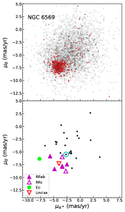
Figure 6: As in Fig. 3, but for NGC 6626 (M 28) in the top panels, for NGC 6569 in the central panels, and for NGC 6441 in the lower panels. Now cyan empty circles encapsulate those variable candidates whose memberships to the cluster according to our kNN classifier were reversed (see text).

In the right panels of Fig. 6 we present the CMDs for these GGCs out to their tidal radii. Since they are contaminated by field stars, we overplotted their innermost ($r\leq 1^{\prime}$) stars selected as members by our kNN classifier. We can appreciate that the dimmest evolutionary sequences we reach in our CMDs for the inner regions of M 28, the lower RGB and upper MS of the cluster appear well populated; however, this is not the case for the inner regions of NGC 6569 and NGC 6441, suggesting that for the innermost regions of these 2 GGCs incompleteness for these evolutionary sequences is higher than for M 28 and M 22. This would explain the lower number of detected RR Lyrae and Cepheids close to the cluster center shown in Sect. 5.1 for both NGC 6569 and NGC 6441.

In the left lower panels of Fig. 6 we present the PMs of the variable candidates detected in the fields of the 3 GGCs considered here, highlighting those that our kNN classifier selected as cluster members. There are 28 member variable stars in M 28, 9 in NGC 6569, and 28 in NGC 6441, according to our kNN classifier. When we analyzed their position in the CMD, the bulk of variable candidates seem to agree with their PM membership classification, but a few of them needed their assigned memberships to be reversed. In the case of M 28 (see top panels in Fig. 6), the positions in the CMD of C24 and C71 (unclassified variables), and C19 (RRab) seem more consistent with their classification as field stars. All of these sources have similar PMs and are near the membership limit according to the kNN classifier, which made us discard these as member stars, along with C46 (unclassified), whose PM is also similar. We also discarded 2 other RRab stars, C49 and C66, owing to their positions in the CMD. They are around half a magnitude below the other RRab sources and they do not suffer from significant reddening. On the other hand, we consider another RRab, C1, to be a member of M 28 owing to its position in the CMD, even though the kNN classifier regards it as a field star. We speculate that the projected proximity of this source to the cluster center may influence the accuracy of its reported PM. A similar situation seems to be happening for C1 and C2 in NGC 6441, which we also classified as cluster members even though their PMs are very different from those of the cluster members (see lower panels in Fig. 6). The cases for the RR Lyrae C28 in NGC 6441 and C4 in NGC 6569 are not so extreme. They have PMs closer to the bulk of the stars in their respective GGCs. We classified these as as cluster members according to their position in the CMD even though our kNN classifier considers them to be field stars (see central and lower panels of Fig. 6). Finally, we consider C39 in NGC 6441 to be a field RRc star given its bright magnitude, even though the PM of this source seems to suggest that it belongs to this GGC (see lower panels in Fig. 6).

In the end, based on their PMs and positions in the CMD, and limiting ourselves to the variables stars we detected, we consider cluster members 23 variable stars in M 28 (including 10 RRab and 5 RRc), 10 in NGC 6569 (including 6 RRab and 2 RRc), and 29 in NGC 6441 (including 16 RRab, 2 RRc, and 1 Cepheid). They are identified as such in Tables 5, 6, and 7, respectively. Their corresponding light curves are shown in Figs. 7, 8, and 9.

Figure 7: As in Fig. 4, but now for variable candidates in the M 28 field selected as cluster members, as shown in Sect. 5.2.

Figure 8: As in Fig. 4, but now for variable candidates in the NGC 6569 field selected as cluster members, as shown in Sect. 5.2.

Figure 9: As in Fig. 4, but now for variable candidates in the NGC 6441 field selected as cluster members, as shown in Sect. 5.2.

5.3 Distance and extinction

The GGCs in this section show a wide range of iron contents (see Table 1). Taking [${\alpha}$/Fe]=0.3 for all of the GGCs (Villanova et al., 2017; Johnson et al., 2018; Origlia et al., 2008) translates into metallicities $Z_{M28}$=0.0013, $Z_{NGC6569}$=0.0048, and $Z_{NGC6441}$=0.0096, using Eq. (1) in Navarrete et al. (2017a). Applying the newly calibrated Paper I PLZ relations from Sect. 4.3 (Eqs. [3] to [7]) to the RR Lyrae selected in Sect. 5.2 as cluster members (15 in M 28, 8 in NGC 6569, and 18 in NGC 6441), and assuming a Cardelli et al. (1989) canonical extinction law toward these as well, we obtain the color excesses and distances for M 28, NGC 6569, and NGC 6441 that we report in Table 4.

The reported distances agree, within the error, with those reported by Baumgardt et al. (2019) using Gaia data, and also with those in the Harris catalog (see Table 4). NGC 6441 is the only case that seems to be off ($\sim 10\%$). This may imply that the uncommon Oosterhoff III GGCs follow different PLZ relations, a very plausible posibility if we consider that the atypical extension of the HB and the long periods in the RR Lyrae in Oosterhoff III GGCs may be attributed to an overabundance of helium (e.g., Caloi & D’Antona, 2007; Catelan, 2009; Tailo et al., 2017), which, as shown in Catelan et al. (2004), significantly impacts the PLZ relations that are followed by RR Lyrae stars.

The dispersion among the distance moduli to individual RR Lyrae in every GGC is small (see Fig. 10). It is unlikely to be due to differential reddening because extinction is relatively low in the near-infrared for these GGCs (see Table 4), and the dispersion among the stars does not seem to follow the reddening vector (e.g., C28 for M 28 or C13 for NGC 6569 in Fig. 10). This dispersion is quoted in Table 4 as the first ${\sigma}$ in our distance determination. Interestingly, this dispersion is similar for NGC 6441 as for the other GGCs.

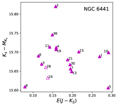
Figure 10: As in Fig. 5, but for NGC 6626 (M 28) in the left panel, for NGC 6569 in the middle panel, and for NGC 6441 in the right panel.

We note that assuming a non-canonical extinction law such as those reported for the innermost Galaxy (e.g., Majaess et al., 2016; Alonso-García et al., 2017; Nogueras-Lara et al., 2018; Dékány et al., 2019) results in increasing the distances to these GGCs. Variations in the distance due to applying such extinction laws are included in the reported second $\sigma$ of the distance estimation in Table 4. We also note that applying the different PLZ relations shown in Sect. 4.3 only produces small variations among the reported mean ${\mu}_{Ks}$ for every cluster, increasing their values from a few hundredths of a magnitude, in the case of the newly calibrated Navarrete et al. (2017b) PLZ relations (Eqs. [1] and [2] in Sect. 4.3), up to $\sim 0.1$ mag, for the Muraveva et al. (2015) PLZ relation. Variations in the distance due to applying these different PLZ relations are included in the reported third $\sigma$ of the distance estimation in Table 4.

There are no Cepheids in M 28 and NGC 6569 that we detected as cluster members, but there is one, C34, in NGC 6441. When we examined its colors, we found it was saturated in $H$ but not in $J$. Using the PL relations by Dékány et al. (2019), we found a color excess $E(J-K_{s})=0.27$ for this Cepheid, and a distance of $R_{\odot}=13.3$ kpc, in agreement with those reported by the RR Lyrae for this GGC (see Table 4), but significantly higher than that reported by Gaia and in the Harris catalog. Therefore, this result hints that a different calibration for the PL relations in Cepheids from Oosterhoff III GGCs may also be required.

6 2MASS-GC 02 and Terzan 10

2MASS-GC 02 and Terzan 10 are different from the previously analyzed GGCs because they are two poorly populated GGCs located at very low latitudes (see Table 1). Their Galactic locations make them two of the most reddened GGCs in the Milky Way. We studied the variable populations in these GGCs and in their immediate surroundings in Paper I. Now we revisit these two GGCs as test cases of our redesigned method to detect variables.

6.1 Variables in the cluster area

2MASS-GC 02 is one of the very few Galactic GGCs lying in the Oosterhoff gap, as we showed in Paper I. We detected 45 variable candidates in its field, following the procedures detailed in Sect. 3. We present their main observational parameters in Table 8. Owing to its position, very close to the Galactic plane, this GGC is outside the footprint of the OGLE experiment. There are 6 variable candidates listed in the Clement catalog, but we discarded these as not being real variables in Paper I. We do not register any signal of variability for these stars in our current analysis either. In Paper I we were able to detect 32 variables inside the tidal radius of this GGC. We independently recovered all the variable stars detected in Paper I, except those classified as long period variables (LPVs): NV16, NV19, and NV27; and the eclipsing binary NV32. This is expected as we explained in Sect. 3: Our method is now restricted to looking for stars with periods shorter than 100 days, and therefore we do not expect to find any LPVs; as for the eclipsing binaries, we expect to miss some of these because of the preliminary cuts we apply to our selection. We underline that we recovered all 16 pulsators (13 RRab’s and 3 Cepheids) previously found in Paper I inside the tidal radius of this GGC. Additionally, we note that the coordinates for the cluster center we used in this work (see Table 1) are slightly different from those assumed in Paper I, which puts the Cepheid candidate C45 (NV33) inside the tidal radius, and among our detected variables. On the other hand, however, the improved light curve of C40 (NV28) casts some doubts on our previous classification as a Cepheid, and we prefer not to assign this source a variable type. Finally, we highlight that there are 16 newly detected candidates. We classified 2 as RRab, 4 as eclipsing binaries, and we were not able to assign a variable type to the other 10 new candidates.

Table 8: Properties of the variable candidates in 2MASS-GC 02.

ID	$ID_{PaperI}$	$\alpha$ (J2000)	${\delta}$ (J2000)	Distance	Period	$A_{K_{s}}$	$\langle K_{s}\rangle$	$Z-K_{s}$	$Y-K_{s}$	$J-K_{s}$	$H-K_{s}$	$\mu_{\alpha^{\ast}}$	$\mu_{\delta}$	Member	Type
		(h:m:s)	(d:m:s)	(arcmin)	(days)	(mag)	(mag)	(mag)	(mag)	(mag)	(mag)	(mas/yr)	(mas/yr)
C1	NV1	18:09:35.98	-20:47:11.7	0.52	0.70004	0.298	14.585	–	4.411	2.783	0.95	4.89	-4.81	Yes	RRab
C2	NV2	18:09:34.22	-20:46:56.2	0.68	0.651668	0.218	14.779	–	–	2.942	1.008	3.785	-4.757	Yes	RRab
C3	NV4	18:09:38.58	-20:46:05.0	0.75	0.623721	0.243	15.356	–	–	4.176	1.494	4.421	-2.921	Yes	RRab
C4	NV3	18:09:33.77	-20:46:29.5	0.79	0.570441	0.279	15.069	–	–	3.46	1.155	5.01	-3.961	Yes	RRab
C5	NV5	18:09:38.85	-20:47:26.5	0.83	0.603305	0.33	14.973	–	–	3.213	1.099	3.846	-3.893	Yes	RRab
C6	NV6	18:09:33.00	-20:47:07.8	1.02	0.551335	0.404	14.965	–	–	2.937	1.004	3.038	-6.488	Yes	RRab
C7	–	18:09:38.86	-20:45:46.7	1.05	0.60917	0.23	15.557	–	–	–	1.758	2.888	-2.794	Yes	RRab
C8	–	18:09:33.46	-20:47:32.9	1.16	1.068307	0.081	14.747	3.327	2.277	1.412	0.503	-2.931	-0.364	No	?
C9	–	18:09:40.77	-20:47:43.5	1.33	3.2458	0.271	14.507	3.734	2.591	1.594	0.537	0.486	-1.929	No	Ecl
C10	–	18:09:31.65	-20:47:24.7	1.42	0.596172	0.34	14.687	–	–	2.924	1.018	3.094	-5.215	Yes	RRab

Terzan 10 shows in Paper I mean periods for its RRab star corresponding to an Oosterhoff II GGC. But its reported metallicity at the time, from photometric measurements, $[{\rm Fe/H}]=-1.0$ according to the Harris catalog, was too high for this group, putting it closer to the Oosterhoff III GGCs. As shown in Table 1, in this paper we use a lower iron content, $[{\rm Fe/H}]=-1.59\pm 0.02$, which is measured from Ca triplet spectra in a sample of 16 member stars observed with the FORS2 instrument at the Very Large Telescope (VLT; Geisler et al., in prep.). This metallicity is more consistent with Terzan 10 being a member of the Oosterhoff II GGCs. We detected 65 variable candidates in its field. We present their main observational parameters in Table 9. The Clement catalog for this GGC shows the variable stars we detected in Paper I, plus a few more candidates from OGLE. There are 48 variable stars listed in Paper I inside the tidal radius of Terzan 10. We recovered all but 7 of these variables: 1 LPV (NV48), since our method is now restricted to looking for stars with periods shorter than 100 days (see Sect. 3); and the other six – 3 variable sources of unknown type (NV8, NV37, and NV38), 2 Cepheid candidates (NV19 and NV39), and 1 eclipsing binary candidate (NV45)–, whose light curves quality was too low to be picked out by our improved method. We note that, as for 2MASS-GC 02, the coordinates for the cluster center we used in this work (see Table 1) are slightly different from those assumed in Paper I for this GGC, which puts NV50 and NV51 from Paper I inside its tidal radius, and among our detected variables. We also reconsidered our previous classifications for some of these stars based on their improved light curves: we classified C56 (NV44) as an RRab, while we were not able to assign a variable type to all the 6 stars (C15, C16, C18, C19, C47, and C54) previously classified as Cepheid candidates (NV16, NV18, NV14, NV17, NV31, and NV47). Finally, there are 22 variable candidates not reported in Paper I that we detected in this work. From those, OGLE previously detected 12 variable stars and the other 10 are newly detected candidates. We classified 2 of them as eclipsing binaries, and we were not able to assign a variable type to the other 8 new candidates.

Table 9: Properties of the variable candidates in Terzan 10.

ID	$ID_{Clement}$	$ID_{OGLE}$	$\alpha$ (J2000)	${\delta}$ (J2000)	Distance	Period	$A_{K_{s}}$	$\langle K_{s}\rangle$	$Z-K_{s}$	$Y-K_{s}$	$J-K_{s}$	$H-K_{s}$	$\mu_{\alpha^{\ast}}$	$\mu_{\delta}$	Member	Type
		(OGLE-BLG-)	(h:m:s)	(d:m:s)	(arcmin)	(days)	(mag)	(mag)	(mag)	(mag)	(mag)	(mag)	(mas/yr)	(mas/yr)
C1	V1	ECL-270713	18:02:58.87	-26:03:35.3	0.46	3.87962	0.39	14.14	2.713	1.833	1.069	0.31	-0.118	-9.19	No	Ecl
C2	V2	RRLYR-33526	18:02:59.48	-26:04:22.6	0.5	0.730538	0.291	14.655	2.734	1.831	1.105	0.331	-6.908	-4.292	Yes	RRab
C3	V3	RRLYR-33512	18:02:54.04	-26:03:46.9	0.92	0.70172	0.298	14.842	3.17	2.005	1.154	0.383	-7.334	-1.237	Yes	RRab
C4	V4	ECL-270954	18:03:00.19	-26:05:05.8	1.2	1.368958	0.395	14.651	2.082	1.421	0.798	0.249	-2.839	-6.769	No	Ecl
C5	V5	–	18:02:57.14	-26:02:44.0	1.28	0.68854	0.314	14.974	3.571	2.522	1.338	0.405	-6.43	-1.814	Yes	RRab
C6	V6	RRLYR-33519	18:02:56.90	-26:05:19.7	1.35	0.582332	0.334	14.957	3.199	2.01	1.14	0.361	-6.184	-2.43	Yes	RRab
C7	V7	RRLYR-33509	18:02:53.24	-26:05:12.7	1.62	0.715331	0.339	14.726	2.928	1.915	1.147	0.409	-8.985	-4.512	Yes	RRab
C8	V10	ECL-271769	18:03:04.65	-26:05:15.4	1.95	0.422508	0.45	16.306	2.033	1.251	0.768	0.221	-4.449	-0.437	Yes	Ecl
C9	V9	–	18:02:51.22	-26:05:14.9	1.97	0.193836	0.236	16.207	2.325	1.605	0.921	0.239	-5.788	-4.402	Yes	?
C10	V12	RRLYR-33538	18:03:04.08	-26:05:33.7	2.07	0.568658	0.291	14.533	2.408	1.7	0.939	0.265	-1.84	-7.808	No	RRab

Therefore, from the analysis of these 2 difficult GGCs, we note that our redesigned method to detect variable candidates (see Sect. 3) recovered all variable stars detected in Paper I, except for those with periods outside of our range of interest and those with low quality light curves. On the other hand, it increased the number of detected candidates with good quality light curves by more than 50 percent. However, we also note that the number of epochs available for our variability analysis was significantly increased with respect to Paper I, by a factor of $\sim 2$ in 2MASS-GC 02 and a factor of $\sim 3$ in Terzan 10.

6.2 Proper motions, color-magnitude diagrams, and cluster memberships

Following the same method described in Sect. 4.2 and 5.2, we used the PMs provided by VIRAC2 for the detected variable stars to assign membership to 2MASS-GC 02 and Terzan 10. In the left upper panels of Fig. 11, we can observe that the PM distributions of stars from both GGCs are more clearly separated from their field counterparts than in the GGCs from the previous section (see Fig. 6). Our kNN classifier allowed us to further select the innermost stars that belong to the GGCs. We are able to obtain in this way the PMs for 2MASS-GC 02 and Terzan 10, which we show in Table 3. While the mean PM for Terzan 10 agrees with that measured by Baumgardt et al. (2019), this is not the case for 2MASS-GC 02. We attribute this to the very high reddening in front of 2MASS-GC 02, which may have produced a wrong identification of its members using Gaia data by Baumgardt et al. (2019). We argue that our VVV near-infrared data for this GGC provides more accurate results in this case because a PM pattern for the stars in this GGC, different from the stars in the field, and not observed in the Gaia data, appears clearly in the left panels of Fig. 11 for 2MASS-GC 02.

Figure 11: As in Fig. 3, but now for 2MASS-GC 02 in the top panels and for Terzan 10 in the lower panels. For 2MASS-GC 02, a cyan empty circle encapsulates the variable candidate whose membership to the cluster according to our kNN classifier was reversed (see text).

Our kNN classifier also allows us to identify cluster member variable stars using their PMs (see left lower panels of Fig. 11). There are 15 variable stars identified as members for 2MASS-GC 02, all of which are RRab stars, except for 1 unclassified variable (C21). However, as the position of C21 in the CMD is too blue to belong to this GGC and better agrees with a star in the foreground disk (see top right panel in Fig. 11), we decided to consider it a non-member in its classification in Table 8. On the other hand, all the RRab classified as cluster members consistently fall along the reddening vector in the CMD, indicating the presence of strong differential reddening in the line of sight of this GGC. All the RRab selected as members in Paper I were also selected in this work using the kNN classifier. We present their $K_{s}$ light curves in Fig. 12. When also considering the additional 2 newly detected RR Lyrae in this GGC, the Oosterhoff intermediate classification we assigned it in Paper I is reinforced. For Terzan 10, our kNN classifier identifies 14 variable stars as cluster members based on their PMs. We present their $K_{s}$ light curves in Fig. 13. As for 2MASS-GC 02, all the RRab stars classified in Paper I as cluster members are also classified as members now.

Figure 12: As in Fig. 4, but now for variable candidates in the 2MASS-GC 02 field selected as cluster members, as shown in Sect. 6.2.

Figure 13: As in Fig. 4, but now for variable candidates in the Terzan 10 field selected as cluster members, as shown in Sect. 6.2.

6.3 Distance and extinction

For our determination of distances and extinctions to 2MASS-GC 02, we used 14 RRLyrae: the 12 cluster members detected in Paper I (C1 to C6, C13 to C16, C19, and C34), plus 2 additional new detections from our current analysis (C7 and C10), which our kNN classifier also considers members of 2MASS-GC 02. The remaining RRab, C38, and the 3 detected Cepheids (C17, C43 and C45) were classified as field stars in Paper I and in this work by our kNN classifier. As mentioned in Sect. 6.2, the positions of the RRab stars of 2MASS-GC 02 in the CMD (see top right panel in Fig. 11) provided us with a clear hint of the significant differential reddening present in the field of this GGC. When we applied the PLZ relations, assuming a metallicity of Z=0.0025 as in Paper I, we could also see the effect of differential extinction in the calculated distance moduli and color excesses (see left panel in Fig. 14). This allowed us to perform an analysis similar to that in Paper I, where we calculated simultaneously extinction ratios and distance to this GGC from a linear fit to the distance moduli and color excesses of its RR Lyrae. The zero-point of the fit is the distance modulus to this GGC, corrected by extinction, while the slope of the fit is the selective-to-total extinction ratio. Unfortunately, as was the case in Paper I, the substantial reddening of 2MASS-GC 02 prevented our detection of the RR Lyrae in the bluer filters ($Z$ and $Y$), so we could only perform our analysis using $J$, $H$, and $K_{s}$. Hence, following Paper I, we performed an ordinary least-squares bisector fit on the $\mu_{K_{s}}$ versus E($J-K_{s}$) and on $\mu_{K_{s}}$ versus E($H-K_{s}$) values obtained from the PLZ relations for the RRab stars and we obtained the selective-to-total extinction ratios $R_{K_{s},H-K_{s}}=1.13\pm 0.11$ and $R_{K_{s},J-K_{s}}=0.55\pm 0.08$, which agree within the errors with those from Paper I. However, we should note that while $R_{K_{s},H-K_{s}}$ is slightly lower than in our previous work, $R_{K_{s},J-K_{s}}$ is instead slightly higher. The mean of the distance moduli corrected by extinction obtained from both fits is $\mu_{0}=13.9\pm 0.3$ mag, which translates into the distance given in Table 4. While this distance differs from that provided by the Harris catalog, it closely agrees with the distance provided in Paper I, once the effects of the recalibration of the PLZ relations are taken into consideration. The color excesses reported in Table 4 for 2MASS-GC 02 are the mean of those obtained to the individual RR Lyrae, and they are similar to those reported in Paper I. However, we note that these average color excesses for 2MASS-GC 02 should be used with caution because extinction toward this GGC is highly variable and changes significantly over small regions.

Figure 14: As in Fig. 5, but now for 2MASS-GC 02 in the left panel and for Terzan 10 in the right panel. Also shown as a straight line for 2MASS-GC 02 is the linear fit used to define its distance modulus corrected by extinction, as the zero-point of the fit, and its selective-to-total extinction ratio, as the slope of the fit.

For Terzan 10, we identified 7 RRab stars as cluster members following the analysis in Sect. 6.2, as we can observe in Fig. 11 and 13. They are the same 7 RRab that we identified in Paper I as members. In the right panel of Fig. 14, we show the distance moduli and color excesses that we obtained after applying the PLZ relations, taking now $Z_{Terzan10}$=0.0007; this is a lower metallicity than inferred in Paper I, which we adopted for this work given the lower iron content for this GGC reported in Table 1. There is indication of differential reddening, but it is less significant than in 2MASS-GC 02. Importantly, the bulk of the RR Lyrae in this GGC does not seem to be suffering from it, with only a couple of these sources (C24, C5) showing significant departures from the mean reddening. So instead of performing a linear fit that would be heavily affected by the extreme values of the color excesses of just these two stars, we preferred to apply the ratios $R_{K_{s},\lambda-K_{s}}$ from Alonso-García et al. (2017) to correct for extinction and calculate their distances. The mean of these measurements is presented in Table 4 as the distance to Terzan 10, and although it is clearly off from the value given in the Harris catalog, this value agrees with that provided in Paper I and also agrees with recent measurements by Ortolani et al. (2019).

7 Conclusions

Using the VVV survey, we studied for the first time in the near-infrared the variable stellar population over the entire field of M 22, M 28, NGC 6569, and NGC 6441, four massive GGCs located toward the Galactic bulge, whose corresponding metallicities span a wide range of values. We also revisited the topic in 2MASS-GC 02 and Terzan 10, which are two poorly populated and highly reddened GGCs we already studied in the first paper of this series. The updated VIRAC2 database provided us with PMs and light curves for the stars located in these GGCs. We defined a parameter that allows us to efficiently discriminate the light curves provided by the VIRAC2 database and to single out those which show clear signs of variability. We were able to identify almost all of the RRab pulsators reported in other catalogs of variable stars for these GGCs, except for the innermost regions of the farthest clusters. Moreover, we were able to catalog some other known RRc and Cepheid pulsators, and some other known binary stars that show clear signs of variability in our VVV dataset, and we identified some tens of new variable candidates. We were also able to recover the vast majority of the variable candidates found for 2MASS-GC 02 and Terzan 10 in the first paper of this series, plus a significant number of new candidates. We used the PMs that VIRAC2 provides to identify cluster members through a kNN classifier. We were able to provide in this way the PMs for these GGCs, which agreed with those provided by Gaia DR2, except for the most reddened cluster, 2MASS-GC 02, where the VVV near-infrared observations provide a more accurate result. Using their PMs, along with their positions in the sky and in the CMD, we were able to select the variable stars that belong to these GGCs as well. Since all of these clusters have a significant number of RR Lyrae, we used their tight, near-infrared PLZ relations to calculate the distances and extinctions toward these GGCs. We recalibrated previously used PLZ relations, obtaining in this way a good agreement with those distances provided in the literature and by Gaia DR2, except in the case of the Oosterhoff III GGC NGC 6441. Building on the methods described in this work, we plan to extend the study of their variable stellar population to the other GGCs located in the footprints of the VVV and the VVVX surveys.