SimNet: Accurate and High-Performance Computer Architecture Simulation using Deep Learning

Abstract.

While cycle-accurate simulators are essential tools for architecture research, design, and development, their practicality is limited by an extremely long time-to-solution for realistic applications under investigation. This work describes a concerted effort, where machine learning (ML) is used to accelerate microarchitecture simulation. First, an ML-based instruction latency prediction framework that accounts for both static instruction properties and dynamic processor states is constructed. Then, a GPU-accelerated parallel simulator is implemented based on the proposed instruction latency predictor, and its simulation accuracy and throughput are validated and evaluated against a state-of-the-art simulator. Leveraging modern GPUs, the ML-based simulator outperforms traditional CPU-based simulators significantly.

1. Introduction

Adopted extensively in computer architecture research and engineering, cycle-accurate discrete-event simulators (DES) enable new architectural ideas, as well as design space exploration. DES is composed of distinct modules that mimic the behavior of different hardware components. On certain events (e.g., advancing a cycle), these individual components and their interactions are simulated to imitate the behavior of processors. Unfortunately, DES is extremely computationally demanding, markedly diminishing its practicality and applicability at full system and application scales. Typical simulations using the state-of-the-art gem5 simulator (Binkert et al., 2011) execute at speeds of hundreds of kilo instructions per second on modern CPUs, about four to five orders of magnitude slower than native execution. In this context, it would require weeks or months to simulate a realistic application that only takes a couple minutes to execute on real hardware. To expand the practical limits of traditional simulation, design space exploration necessitates a multitude of simulations across various applications and design parameters under consideration.

Many efforts have been made to improve traditional simulation speed through software engineering optimizations (Sandberg et al., 2015; Jaleel et al., 2008; Patel et al., 2011), multi/many-core simulation parallelization (Janssen et al., 2010; Sanchez and Kozyrakis, 2013), and statistical approaches (Sherwood et al., 2002; Perelman et al., 2003; Wunderlich et al., 2003). Among them, parallelization is a promising direction due to the broad availability of massive parallel accelerators such as GPUs nowadays. However, one fundamental limitation of these traditional simulators is they are intrinsically difficult to parallelize because of the heterogeneous nature of distinct components, frequent interactions between components, and irregular behaviors. As a result, existing parallel simulators focus on a coarse parallelization strategy, where the simulation of individual cores is parallelized (Janssen et al., 2010; Sanchez and Kozyrakis, 2013). These simulators have limited scalability and cannot leverage modern parallel accelerators.

In the meantime, machine learning (ML) advances have led to remarkable achievements in many domains, and using ML for analytical performance modeling is significant and growing. Considerable research has been done to predict application performance (Ïpek et al., 2006; Lee and Brooks, 2007; Lee et al., 2007; Agbarya et al., 2020; Ardalani et al., 2015; Baldini et al., 2014; O’neal et al., 2017; Zheng et al., 2016). The major limitation of these application-centric methods is they are program/input dependent, which means ML models need to be trained for individual program and input combinations. As a result, their flexibility is limited compared to simulation-based approaches.

This paper aims to explore the possibility of an ML-based computer architecture simulation approach given the following reasons. First, ML models, especially deep neural networks, have been proved to be excellent function approximators in many domains, from computer vision to scientific computing (Vaswani et al., 2017; Tan and Le, 2019; Senior et al., 2020; Jia et al., 2020). We expect they can also be applied to approximate the complex and implicit latency calculations that are essential to computer architecture simulation. Second, ML-based simulation is more flexible compared with ML-based analytical modeling because it does not require training per program/input. Moreover, an ML-based simulator could bring performance advantages because ML inferences are highly parallel, and state-of-the-art accelerators (e.g., GPU; TPU (Jouppi et al., 2017)) and software infrastructures (Paszke et al., 2019; Abadi et al., 2016; Vanholder, 2016) are well optimized for such tasks.

Motivated by these potentials, we establish the first ML-based architecture simulator, SimNet. SimNet is a novel instruction-centric simulation framework that decomposes program simulation into individual instruction latency and uses tailored ML techniques for instruction latency prediction. Program performance is obtained by combining the latency prediction results of all executed instructions. SimNet achieves noticeably higher simulation throughput while maintaining the same level of simulation accuracy because: 1) it abstracts the simulated processor as a whole and eliminates the need to simulate individual components within the processor, and 2) it is well optimized to execute on GPUs efficiently. Moreover, SimNet can simulate complex processor architectures and realistic application workloads with billions/trillions of instructions. The source code of SimNet is available at https://github.com/lingda-li/simnet.

This work’s contributions to the science and practice of simulation include:

• We propose an ML framework to predict instruction latency accurately (Section 2). The proposed framework accounts for both static instruction properties and dynamic processor behaviors, and extensive ML models are evaluated to balance between the prediction accuracy and speed.

• We propose an instruction-centric architecture simulator that is built upon ML-based instruction latency predictors (Section 3). Evaluated using a realistic benchmark suite and on full microprocessor architectures, we demonstrate that the proposed approach simulates programs faithfully compared with the discrete-event simulator it learns from. To the best of our knowledge, the proposed framework is the first of its kind and could set the stage for developing alternative tools for architecture researchers and engineers.

• We also prototype a GPU-accelerated ML-based simulator (Section 3.3). It improves the simulation throughput up to $76\times$ compared to its traditional counterpart. It also achieves a higher throughput per watt thanks to GPU’s power efficiency advantage.

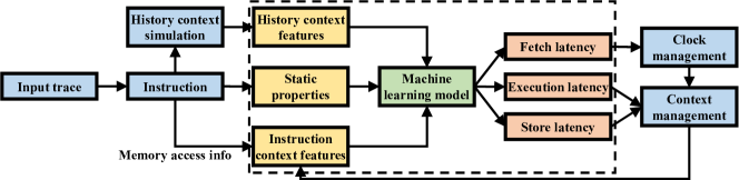
Figure 1. ML-based simulation workflow. The ML-based instruction latency predictor is shown in green, and its input and output are in yellow and orange, respectively (Section 2). Other simulator components are in blue (Section 3).

Related Work. Ithemal (Mendis et al., 2019) represents the closest related work to this effort, proposing a long short-term memory (LSTM) model to predict the execution latency of static basic blocks. However, Ithemal has three major limitations: 1) it targets a simplified processor model without branch prediction and cache/memory hierarchies; 2) it can only predict the performance of basic blocks with a handful of instructions, while real-world simulation executes billions or trillions of instructions; and 3) it simulates instructions at a pace of thousands of instructions per second, which is significantly slower than traditional simulators. As a result, unlike SimNet, Ithemal can neither simulate real-world processors nor applications, and it is infeasible for realistic computer architecture simulation. Section 2.5 will quantitatively compare Ithemal with SimNet, and Section 6 will discuss other related works.

Scope of Work. This paper focuses on simulating out-of-order superscalar CPUs, which employ technologies such as multi-issue, out-of-order scheduling, and speculative execution to exploit instruction-level parallelism. We posit the proposed simulation methodology also is applicable to other processor architectures, which usually are less challenging to simulate. In addition, we constrain the scope to the prediction of program performance and single-thread program simulation, leaving multiple-thread/program simulation for future work. Traditional simulators also produce additional metrics other than performance, such as energy consumption. While it is reasonable to assume the proposed method is applicable to such prediction as well, these metrics are not considered in this work.

2. ML-based Latency Prediction

Figure 1 shows the workflow of SimNet. SimNet is built around an ML-based instruction latency prediction framework (the dashed box in Figure 1), and this section will describe its design.

2.1. Factors that Determine Instruction Latency

Successful instruction latency prediction by an ML model is contingent upon capturing all factors that impact latency in its design and implementation. These factors can be summarized into three categories.

Static Instruction Properties. These properties describe the basics of an instruction, including the operation types, source/destination registers, etc. They guide how an instruction is executed in a processor. For instance, the type of instruction determines its computation resource (e.g., function units; register files) and synchronization requirements (e.g., memory barriers).

Dynamic Processor States. Besides its static properties, the latency of an instruction largely depends on the states of all processor components (e.g., register files; caches) at its execution time. We refer to these states as contexts and further distill them into two categories.

Instruction Context: Many contexts relate to other concurrently running instructions in the processor, referred to as instruction context in this paper. For example, whether the desired execution unit is available depends on whether there is a co-running instruction of the same type using it currently, and if a source register can be read immediately depends on whether the previous instruction that writes the same register has finished. We argue that instruction context can be determined given all concurrently running instructions, named context instructions in this paper. The processor capacity decides the maximal number of context instructions.

History Context: The remaining hardware contexts depend on events that happened in the long-term execution history. Cache, translation lookaside buffer (TLB), and branch predictor states belong to this category. For example, whether a memory load hits in the L2 cache depends on when the same cache line was last accessed, and branch prediction results hinge on the branch execution history. Traditional simulators employ lookup tables (e.g., cache tag array; branch target predictor) to keep track of such states. We refer to them as history context.

2.2. Framework Formulation

Impact Factor	Features
Static properties	13 operation features (function type, direct/indirect branch, memory barrier, etc.); 14 register indices (8 sources and 6 destinations)
Instruction context	27 static properties; 14 history context features; 1 residence latency; 1 execution latency; 1 store latency; 5 memory dependency flags to indicate if it shares the same instruction/data address/cache line/page with the current instruction
History context	1 branch misprediction flag; 1 fetch level; 3 fetch table walking levels; 2 fetch caused writebacks; 1 data access level; 3 data access table walking levels; 3 data access caused writebacks

Table 1. Input features for various instruction latency impact factors.

With these impact factors, we are ready to build an instruction latency prediction framework. The framework aims to balance between two competing goals: to predict instruction latency accurately and swiftly. An ML-based instruction latency predictor (the green box in Figure 1) is the center of the framework, which captures the impact of input features. Its inputs (yellow boxes) take into account the aforementioned impact factors. Table 1 summarizes the input features, which are divided into three categories based on which impact factor they model as introduced below.

Modeling Static Instruction Properties. The top row of Table 1 lists the static instruction properties used as the input features of the ML model, including 13 operation features and 14 source and destination register indices. They are well known to computer architects and can be extracted from the instruction encoding directly.

Modeling Instruction Context. To account for the impact of concurrently running instructions, the key is to model their relationships with the to-be-predicted instruction. Such relationships include resource competition, register dependency, and memory dependency. We call these concurrently running instructions, context instructions. Formally, the context instructions are those instructions present in the processor when a particular instruction is about to be fetched. In theory, instructions issued after the current instruction also can influence its execution. However, these cases are rare, and we only include previous instructions for practicality. The middle row of Table 1 shows input features per context instruction.

For resource competition and register dependency, it is sufficient to provide the static properties of context instructions (i.e., their operation features and register indices). The ML model is responsible for deducing the resource competition using their operation features and the register dependency by comparing register indices.

To model the memory dependency (including instruction fetch and data access), one solution is to provide memory access addresses as parts of input features and leave the rest work to the ML model. Unlike register indices, memory access addresses spread across a much wider range in a typical 64-bit address space. Thus, having addresses as input would slow down the ML model prediction speed. Instead, we extract the memory dependency by explicitly comparing the memory access addresses of the current instruction with those of context instructions and generate several memory dependency flags as input features. For example, we compare their program counters (PCs) to identify if they fall into the same instruction cache line. This PC dependency flag presumably helps with fetch latency prediction as instructions that share the same instruction cache line can be fetched together. Similarly, there are dependency flags to indicate if data accesses share the same address, cache line, and page.

In addition, we introduce several features to capture the temporal relationship between instructions. Particularly, we include the number of cycles it has stayed in the processor (i.e., residence latency), how long it takes to complete execution (i.e., execution latency), and the memory store latency (i.e., store latency) if applicable. The latter two are provided by the ML model output, which will be introduced shortly. The latency of context instructions is useful to predict the latency of the current one. For example, when an instruction follows a mispredicted branch, its fetch latency is decided by the execution latency of the branch.

Modeling History Context through Simplified Simulation. History context reflects the hardware states that depend on long-term historical events, and it includes caches, TLBs, and branch predictors. It is impractical to either capture the history context within the ML model or directly have it as the input because it includes a huge amount of information. Considering a 2MB cache with 64B cache lines as an example, we will need $\sim$5B per cache line to store its address tag, etc. Totally, a 2MB cache requires storing at least $2\text{MB}\div 64\text{B}\times 5\text{B}=160\text{KB}$ of information to simulate it accurately. The total history-context-related information is much larger given all history context. It is prohibitively expensive and inefficient to let the ML model memorize such large amounts of information.

Fortunately, the majority of history context impacts can be captured using a small number of intermediate results. For a memory access, the cache/TLB level in which it gets hit roughly determines its latency. Similarly, whether or not a branch target is predicted correctly determines the impact of a branch prediction.

Therefore, we propose to simulate history context components explicitly to obtain these intermediate results (i.e., history context simulation), which are passed to the ML model as input features. History context simulation greatly alleviates the burden on ML models. As shown in the last row of Table 1, a branch misprediction flag is obtained for a branch instruction. An access level feature is used for each memory access to indicate which level of the cache/TLB hierarchy satisfies the request. All instructions require fetch access and fetch table walking levels, and load/store instructions need data access and data table walking levels, e.g., a load request that hits in the L2 cache has a level of 2. The numbers of cache writebacks generated are also included in input features to capture their impacts.

Note that obtaining these intermediate results mostly involves table lookups (e.g., cache tag array; branch direction predictor). Detailed structures, such as pipeline and miss status history register (MSHR), are not needed in the history context simulation. The impacts of these structures are captured by the ML model in SimNet. Therefore, the history context simulation is lightweight and has negligible impact on the overall performance.

ML Model Input Summary. In total, each context instruction has 50 input features, and the to-be-predicted instruction has 47 input features. For alignment purposes, we pad the to-be-predicted instruction features with three zeros, to have an equal number of 50 features. Together, the ML model takes $50\times(\text{\# context instructions}+1)$ features as input. While it is common to adopt one-hot encoding for individual input features, we choose not to do so to favor smaller input size and faster prediction speed.

ML Model Output. In Figure 1, the ML model is designed to predict three types of latencies per instruction: fetch, execution, and store. Fetch latency represents how long an instruction needs to wait to enter the processor after the previous instruction is fetched. It is affected by both its instruction fetch request and context instructions (e.g., when it follows a mispredicted branch). Execution latency represents the time interval from when an instruction is fetched to when it finishes execution and is ready to retire from the reorder buffer (ROB). Note it is different from the ROB retire latency because the ROB retires instructions in order. For store instructions, they write memory after being retired from the ROB. The store latency is used to represent the latency from when a store instruction is fetched to when it completes memory write (i.e., when it is ready to retire from the store queue (SQ)). Section 3.1 will introduce how these latencies are used in SimNet simulation.

2.3. Neural Network Architecture

Given the input and output, we train various ML models to learn their connections and capture the architectural impact.

Sequence-Oriented Models. The ML model input includes a sequence of instructions (i.e., to-be-predicted instruction and context instructions), similar to word sequences in the case of natural language processing (NLP). Therefore, a natural option is to apply models designed to process sequences, such as recurrent neural networks (Rumelhart et al., 1986), LSTM (Hochreiter and Schmidhuber, 1997), and Transformer (Vaswani et al., 2017), for instruction latency prediction. Ithemal (Mendis et al., 2019) follows this strategy and adopts LSTM to predict basic block latency. The main drawback of these models is they are more computational intensive, resulting in low simulation throughput.

Deep Convolutional Neural Network (CNN) Models. Deep CNN models have shown great success in computer vision (Krizhevsky et al., 2012; He et al., 2016; Tan and Le, 2019), where convolution kernels learn and recognize the spatial relationship between pixels. In our instruction latency prediction setting, convolution can help learn the relationship among input instructions. CNNs are less computational demanding than sequence-oriented models and fully connected networks. Another benefit of CNN is it eases the training of deeper networks because significantly less parameters need to be learned. As will be demonstrated in Section 2.5, we choose CNNs for SimNet’s instruction latency predictors due to their prediction accuracy and computation overhead advantages.

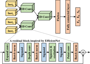
Figure 2. Convolutional neural network architecture illustration.

Figure 2 illustrates the proposed CNN architecture. $\text{Inst}_{0}$ represents the instruction to be predicted, and the ML model outputs $F_{0}$, $E_{0}$, and $S_{0}$, which are its predicted fetch, execution, and store latencies, respectively. Without loss of generality, Figure 2 shows three context instructions, $\text{Inst}_{1,2,3}$.

We organize input instructions in a one-dimensional (1D) array by their execution order and have their features as channels, per CNN terminology. As introduced in Section 2.2, every instruction includes 50 features. Using computer vision as an analogy, instructions correspond to pixels, except they are 1D instead of two-dimensional, and instruction features correspond to pixel color channels. This input organization facilitates convolutional operations to reason the relationship between instructions. Again, it is analogous to reasoning the shape composed by pixels in computer vision.

We organize the convolutional layers in a hierarchical way, where the first layer captures the relationship between temporally adjacent instructions, and subsequent layers integrate the impact of further away instructions. In Figure 2, the impact of $\text{Inst}_{1}$ to $\text{Inst}_{0}$ is captured in the first layer, and the impact of $\text{Inst}_{2}$ and $\text{Inst}_{3}$ is incorporated in the second layer. This hierarchical design prioritizes the impact of temporally closer context instructions while penalizing the influence of more distant instructions, and real processors follow the same principle. For instance, if a source register of $\text{Inst}_{0}$ is the destination register of both $\text{Inst}_{1}$ and $\text{Inst}_{3}$, $\text{Inst}_{0}$ only has to wait for $\text{Inst}_{1}$ where a true read after write dependency exists.

In our default design, each convolution layer includes a convolution operation followed by an activation operation. An alternative is to use a residual block as shown at the bottom of Figure 2, which facilitates to increase the depth of CNNs (He et al., 2016). In this work, we design a residual block architecture inspired by the state-of-the-art image recognition model, EfficientNet (Tan and Le, 2019; Tan et al., 2019).

The output of the last convolutional layer is flattened then used as the input of two fully connected layers. At the end, the model outputs the predicted fetch, execution, and store latencies of $\text{Inst}_{0}$. We adopt the commonly used rectified linear unit (ReLU) as the activation function of both the convolutional and fully connected layers.

Empirically, we find the following CNN design principles work well for instruction latency prediction. First, the inputs of different convolutional operations have no overlap in contrast to computer vision CNNs. For example, we do not convolve $\text{Inst}_{1}$ and $\text{Inst}_{2}$ in Figure 2. In this way, the impact of a context instruction is integrated only once. Second, a convolution kernel size of 2 is always used to account for only two adjacent inputs, which reduces the complexity. Combined with the first principle, it means all convolutional layers have the uniform kernel and stride size, 2. Our experiments demonstrate that these principles work well across different architecture configurations. While an extensive neural architecture search (Elsken et al., 2019) could potentially find better architectures, it also means significant searching overhead and we leave it for future work.

From Output to Latency. There are two ways to convert the ML model output to the latency prediction results. In a regression model, the model output is directly used as the predicted latency. One inherited issue for the regression latency prediction model is its inability to distinguish between small latency differences. The impact may be minor when a latency of 1000 cycles is predicted to be 1001 cycles, but the error could be significant for small latencies (e.g., 0 cycle predicted to be 1). Because the fetch latency is 0 or 1 cycle in most cases, this drawback is particularly critical for its prediction.

A classification model could help to better distinguish between close latency values, where every latency value corresponds to a class, and the ML model predicts which class has the largest probability. However, because the latency could be up to several thousands of cycles, a pure classification scheme will significantly increase the output size and, thus, the computational overhead. Another problem of a pure classification scheme is it is difficult to train such a model because large latency samples appear less frequently in the training set.

As it is quite expensive to have a class for each possible latency value, we propose a hybrid scheme which uses classification for latency that appears frequently and regression for others. Naturally, small latencies appear more frequently. Taking the fetch latency prediction as an example, we classify them into 10 classes in the hybrid scheme. Cycles 0 to 8 have dedicated classes ($c_{0},...,c_{8}$), while another class is used to represent cycles that are larger than 8 ($c_{>8}$). The proposed model outputs the probability of each class. It also outputs a direct prediction result $l$ as in the regression model. On a prediction, we first check which class has the largest probability. If it is one among $c_{0},...,c_{8}$, the corresponding latency is predicted. Otherwise, $l$ is used as the predicted latency. Similar procedures are used to predict execution and store latencies.

2.4. Dataset and Training

Data Acquisition. Due to their data-driven nature, acquiring a sufficient training dataset is necessary for the success of ML-based approaches. Fortunately, it is convenient to engage existing simulator infrastructures to acquire a dataset for standard supervised training.

We modify gem5 (Binkert et al., 2011) to dump instruction execution traces, which then are used to generate ML training/validation/testing datasets. In the modified gem5, each instruction is assigned with three timestamps to record its respective fetch, execution, and store latencies. While the fetch latency stamp is updated in the instruction fetch unit, the execution and store latency stamps are updated in the ROB and SQ, respectively. After all latencies of an instruction are recorded, gem5 dumps it to a trace file.

The instruction traces output by gem5 require several steps of processing before they can be used for ML. First, for each instruction, we find and associate its context instructions based on the timestamps to form a sample. Second, many samples may be alike because the same scenarios can appear repeatedly during the execution of benchmarks. We eliminate such duplication to reduce the dataset. Finally, we convert the dataset to the format used by the ML framework.

Parameter	Default O3CPU	A64FX
Core	3-wide fetch, 8-wide out-of-order issue/commit, bi-mode branch predictor, 32-entry IQ, 40-entry ROB, 16-entry LQ, 16-entry SQ	8-wide fetch, 4-wide out-of-order issue/commit, bi-mode branch predictor, 48-entry IQ, 128-entry ROB, 40-entry LQ, 24-entry SQ
L1 ICache	48KB, 3-way, LRU, 4 MSHRs	64KB, 4-way, LRU, 8 MSHRs
L1 DCache	32KB, 2-way, LRU, 16 MSHRs, 5-cycle latency	64KB, 4-way, LRU, 21 MSHRs, 8-cycle latency, 8-degree stride prefetcher
I/DMMU	2-stage TLBs, 1KB 8-way TLB caches with 6 MSHRs	2-stage TLBs, 1KB 4-way TLB caches with 6 MSHRs
L2 Cache	1MB, 16-way, LRU, 32 MSHRs, 29-cycle latency	8MB 16-way, LRU, 64 MSHRs, 111-cycle latency

Table 2. Simulated processor configurations.

Table 2 shows the processor configurations that ML models learn from. The default O3CPU resembles a classic superscalar CPU. We also train models to learn the Fujitsu A64FX CPU deployed in the current top-ranked supercomputer, Fugaku (Yoshida, 2018; Sato et al., 2020), which represents a state-of-the-art CPU. We obtain the official gem5 configurations of A64FX at (Kodama et al., 2019), which is verified to have an average simulation error of 6.6% against the real processor. Both simulated processors support the ARMv8 instruction set architecture (ISA), and benchmarks are compiled using gcc 8.2.0 under the O3 optimization level. The full system simulation mode of gem5 is employed with Linux kernel 4.15. We use the default O3CPU configuration for most of our experiments, while Section 4.1 will present the results for the A64FX configuration. Under the default O3CPU configuration, there are, at most, 110 context instructions. Therefore, the ML model input has $50\times(1+110)=5550$ features.

ARMv8 is a representative 64-bit reduced instruction set computer (RISC). It includes various integer, floating-point, branch/jump, load/store, vectorized floating-point/integer, Boolean logic instructions, etc. A trained SimNet model can predict the latency of all these instructions. We expect SimNet will be able to support future ISA extensions.

SimNet can also support other ISAs including complex instruction set computers (CISCs) such as x86. To directly predict the performance of CISC instructions, more input features (e.g., multiple data access levels) are required because they show more complex behaviors such as multiple memory accesses. Another possible approach to support CISCs is to decompose CISC instructions into RISC like macro instructions, similar to what contemporary CISC CPUs do. In this way, SimNet can be used to predict the latency of simpler RISC instructions, similar to ARM ones.

Benchmark. Theoretically, any program can be run on the modified gem5 to collect the ML dataset, and we can acquire an unlimited amount of data. We choose to use the SPEC CPU 2017 (Bucek et al., 2018) benchmark suite in this paper because it is widely used in computer architecture simulation and includes a wide range of applications, which should lead to a sufficient coverage of instruction execution scenarios. We select the first four SPEC CPU 2017 benchmarks to generate the ML training/validation/testing dataset, which are shown in Table 3. The default test workloads are used for these four benchmarks, and one billion instructions are simulated from the beginning for each benchmark to collect the ML dataset. Totally, we obtain a dataset with 71 million samples, among which roughly 90% of them are dedicated for training, 5% for validation, and 5% for testing.

As will be introduced in Section 4, we use the reference workloads to verify the simulation accuracy of all 25 SPEC CPU 2017 benchmarks. The facts that 21 benchmarks of them do not appear in the ML dataset and the simulation accuracy is evaluated on different input workloads, allow us to evaluate the generalizability of SimNet.

Type	ML	Simulation
INT	perlbench, gcc	mcf, omnetpp, xalancbmk, x264, deepsjeng, leela, exchange2, xz, specrand_i
FP	bwaves, namd	cactuBSSN, parest, povray, lbm, wrf, blender, cam4, imagick, nab, fotonik3d, roms, specrand_f

Table 3. Benchmarks for ML and simulation.

Training. We use the standard gradient-based optimization to train various models. Let $\{(x_{i},y_{i})\}_{i=1}^{n}$ represent the set of input and output pairs in a training set of $n$ samples. Let $f_{\theta}$ represent a to-be-trained model with parameters $\theta$, and our goal is to find a particular $\theta$ that minimizes the training loss $J(\theta)=\frac{1}{n}\sum\limits_{i=1}^{n}L(f_{\theta}(x_{i}),y_{i}).$ When training the regression output, $L$ is the squared-error loss function. When training the classification output, $L$ is the cross-entropy loss function.

Our training code is built upon PyTorch 1.7.0 (Paszke et al., 2019). The objective function $J$ is minimized using the Adam optimizer (Kingma and Ba, 2015). We use a learning rate of 0.001 and no weight decay or momentum. Every model is trained for 200 epochs, and the validation set is used to select the model with the lowest loss. No hyperparameter tuning is performed when training for different architecture configurations to avoid extensive hyperparameter search overhead. Our ML training hardware platform is an NVIDIA DGX A100 system (dgx, 2020). It includes eight NVIDIA A100 GPUs connected through NVLink 3.0 and NVSwitch, and each is equipped with 40GB HBM that supports 1.5 TB/sec peak bandwidth. Tensor cores in an A100 GPU enable a peak performance of 156 TFlops for Tensor Float 32 operations. The DGX A100 system’s high computing and memory throughputs make it ideal for ML training and inference. Depending on its complexity, training a model takes $18\sim 75$ hours on this machine. Section 4.3 will discuss the training overhead.

Approach	ML model	Output	Computation intensity (MFlops)	Instruction prediction error			Benchmark simulation error
				Fetch	Execution	Store	train avg.	sim. avg.	all avg.
SimNet	FC2	reg	5.7	89%	11%	71%	82%	57%	61%
	FC3	reg	6.7	32%	6.1%	4.1%	14%	20%	19%
	C1	reg	4.0	55%	9.3%	8.5%	19%	31%	29%
	C3	reg	8.1	35%	6.4%	17%	4.6%	9.0%	8.3%
	C3	hyb	8.1	2.7%	3.4%	1.0%	2.7%	12%	10%
	RB7	hyb	93	1.7%	1.8%	0.6%	5.7%	5.5%	5.6%
	LSTM2	hyb	119	6.5%	6.0%	1.6%	7.3%	7.9%	7.8%
	TX6	hyb	1185	6.4%	4.2%	1.1%	7.9%	9.6%	9.3%
Ithemal	LSTM2	N/A	216	64%	17%	37%	20%	27%	26%
	LSTM4		487	68%	14%	74%	15%	16%	16%

Table 4. Instruction latency prediction and program simulation accuracy of various ML models. Output indicates if it is a regression model (reg) or hybrid model with classification (hyb). Computation intensity measures the number of million floating point multiplications (MFlops) required for one inference.

2.5. Model Evaluation

We evaluate an array of ML models for instruction latency prediction, and the middle part of Table 4 compares their prediction accuracy. We represent an ML model using a combination of letters and numbers, where the prefix denotes the basic building block type and the suffix denotes the number of layers. Particularly, FC, C, RB, LSTM, and TX represent the fully connected layer, the conventional convolutional layer, the residual block depicted at the bottom of Figure 2, the standard LSTM block, and the Transformer encoder layer (Vaswani et al., 2017), respectively. For example, C3 is composed of three conventional convolutional layers.

The prediction error of each latency type is defined as follows for the $i$th entry of testing dataset: $E=\frac{|f_{\theta}(x_{i})-y_{i}|}{y_{i}+1}$, where $x_{i}$ is the input and $y_{i}$ is the expected output. Note that we use $y_{i}+1$ as the denominator instead of $y_{i}$ because the $y_{i}$ of fetch and store latencies (e.g., non stores) is often 0.

Table 4 affords several observations. First, we note that the prediction error of CNNs improves with the number of layers, which demonstrates the necessity of a deep neural network. Particularly, RB7 with residual blocks achieves the best accuracy, while the simplest FC2 model’s prediction error is an order of magnitude larger.

Second, the hybrid scheme helps reduce prediction errors, from 35% to 2.7% for fetch latency’s error under C3, while barely increasing the computation complexity. We notice that the hybrid C3 model makes correct fetch latency predictions in 95% of cases. In comparison, the regression C3 model predicts 65% of fetch latency correctly, which demonstrates that classification is helpful to predict latencies with small values.

Third, Table 4 also compares the computational overhead of various models. CNN models require $4\sim 93$ millions of multiplications per inference/prediction. Different models represent different trade-off points between accuracy and computation overhead. Although they seem to be higher than that of traditional simulators, these computations are performed very efficiently on modern accelerators, such as GPUs and TPUs. As a result, SimNet achieves significantly higher simulation throughputs as well as better power efficiency, as will be shown in Section 4.2.

Compared with CNN models, both LSTM and Transformer models show lower prediction accuracy while incurring much larger computational overhead. Transformer models are especially expensive due to the attention computation (Vaswani et al., 2017). Although there are spaces to improve their accuracy through the adoption of deeper and wider networks, doing so requires larger computation overhead. This demonstrates that CNNs are more efficient at instruction latency prediction under a constrained computation budget.

Comparison with Ithemal. We also compare SimNet with Ithemal (Mendis et al., 2019), a state-of-the-art ML-based latency prediction approach. It is designed to predict the latency of a basic block for processors with ideal caches and branch predictors, i.e., all memory accesses hit in L1 caches, and branch latency is not considered. To make a meanful comparison, we enhance it with SimNet input features so that it considers the impact of realistic caches and branch predictors and can predict the latencies of instruction sequences that are much longer than basic blocks. The key difference between Ithemal and SimNet is that the former uses a fix number of previous instructions as the input, while the latter explicitly selects instructions that are active in the processor (i.e., context instructions) as its input and excludes those that have retired.

We train two LSTM models using the Ithemal approach, and the last two rows of Table 4 show their results. The LSTM4 model is similar to what Ithemal originally uses, and we also include a 2-layer LSTM. The same training dataset and process as SimNet is adopted to ensure fairness. We find LSTM4 does not always perform better than LSTM2 due to the fading gradient problem that is common for deep LSTM training.

We observe that SimNet’s prediction errors are one order of magnitude lower than those of Ithemal. SimNet models also incur lower computation overhead. These results demonstrate that explicitly constructing context instructions significantly improves instruction latency prediction accuracy, which is a key contribution of SimNet. This conclusion is intuitive because the input can better reflect the processor status when excluding retired instructions, which simplifies the job of ML models and results in higher accuracy. Note that the LSTM2 models of SimNet and Ithemal have the same architecture. SimNet’s LSTM2 has a lower computation intensity because SimNet has less instructions as input. The fact that SimNet’s LSTM2 has significantly better prediction accuracy than Ithemal’s LSTM2 further demonstrates the effectiveness of SimNet.

3. ML-based Simulation

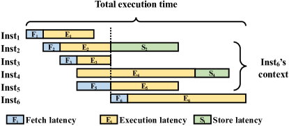
Figure 3. From instruction latency to program execution time.

3.1. From Instruction Latency to Program Performance

SimNet simulates the program performance using the ML-based instruction latency predictor introduced in Section 2. Figure 3 illustrates how to calculate program execution time using instruction latencies, leveraging the fact that instruction fetch and instruction retire from ROB and SQ happen in order. Note that the fetch latency could be 0 in cases when multiple instructions are fetched together (e.g., $\text{Inst}_{4}$). We observe the execution time $\mathcal{E}$ of a program can be computed as

(1) $$\mathcal{E}=(\sum_{i=1}^{n}F_{i})+\Delta,$$

where $n$ is the total number of simulated instructions, $F_{i}$ represents the fetch latency of the $i$th instruction, and $\Delta$ is the amount of time from when the last instruction is fetched to when all instructions exit the processor. When $n$ is large enough, the total execution time is dominated by the accumulated fetch latencies, and $\Delta$ is negligible. This equation lays down the foundation for the proposed instruction-centric simulator.

3.2. Simulator Implementation

Based on Equation 1, we develop a trace-driven simulator. The simulator goes through every executed instruction instance to predict its latency and outputs the program performance upon completion. The modified gem5 is used to generate input traces, which include instruction properties extracted by functional simulation, and history context simulation results.

Context Management. As introduced in Section 2.2, the ML predictor requires the features of context instructions as part of its input. Therefore, SimNet needs to keep track of context instructions. For example, in Figure 3, when $\text{Inst}_{6}$ is about to be fetched (vertical black-dotted line), $\text{Inst}_{1}$ has retired, and $\text{Inst}_{2\sim 5}$ are still in the processor based on their execution and store latencies. Therefore, $\text{Inst}_{2\sim 5}$ are the context instructions of $\text{Inst}_{6}$. To this end, we employ two first-in-first-out (FIFO) queues, processor queue and memory write queue, to keep track of context instructions that stay in the processor and their features. They roughly correspond to the ROB and SQ in an out-of-order processor but are not exactly the same. The two major differences are that the processor queue includes instructions in the frontend, while ROB does not, and a store instruction enters the memory write queue after it retires from the processor queue.

After the simulator reads one instruction from the input trace, the ML predictor is invoked to predict its latency. Then, it enters the processor queue with the residence latency initialized to 0. When it retires from the processor queue is determined based on its predicted execution latency and other simulation constraints (e.g., it must obey the in-order retirement and retire bandwidth). A non-store instruction exits the simulator when it retires from the processor queue. For a store instruction, it will enter the memory write queue. Similarly, when an instruction retires from the memory write queue is decided based on its predicted store latency, and it will exit the processor at that time. Much like real processors, the retire bandwidth of a processor queue is set according to that of the ROB, and the memory write queue can retire any number of instructions from its tail.

Clock Management. The simulator employs curTick to record the total number of simulation cycles, which is updated whenever a prediction completes. When the predicted fetch latency is larger than 0, it is added to curTick so that the counter always points to the time when the current instruction enters the processor. In this case, we also increase the residence latency of all context instructions by the predicted fetch latency to update the time that they have remained in the processor. When the residence latency of an instruction is larger than its execution latency, it is ready to retire from the processor queue. Similarly, an instruction is ready to retire from the memory write queue when its residence latency exceeds its store latency.

After the last instruction in the input trace is predicted, we continue advancing curTick until all instructions retire from the simulator. The final value of curTick represents the total execution time of the program, which is exactly the same as Equation 1.

3.3. GPU-accelerated Parallel Simulation

In our ML-based instruction latency predictor, the latency of an instruction depends on the predicted latencies of previous instructions, i.e., the latency prediction of adjacent instructions is inherently sequential. This restriction limits the sequential simulation speed and computational resource utilization. As a result, a sequential implementation of SimNet runs at a throughput of $\sim$ 1k instructions per second, and it can only leverage a very small fraction of modern GPU’s computing power. To improve the simulation throughput and resource utilization, we seek to extract parallelism.

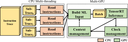
Figure 4. Parallel simulation framework.

Parallel Simulation of Sub-traces. The primary idea is to break down the input instruction trace into multiple, equally sized continuous sub-traces and simulate sub-traces independently in parallel. The instructions within each sub-trace are simulated sequentially to preserve the instruction dependency within the specific sub-trace. The drawback of this approach is that extra simulation errors are introduced when simulating earlier instructions of a sub-trace due to inaccurate or missing contexts. Section 4.2 will show that such accuracy loss is negligible when each sub-trace is large enough. Figure 4 shows the overview of parallel simulation. The design leverages CPU multi-threading to partition the input trace and transfer sub-trace instructions to the GPU memory. The remaining work is done by GPUs to capitalize on their high computational capacity and reduce communications between CPUs and GPUs.

GPU Acceleration. Both context and clock management are implemented on GPUs, and each sub-trace has separate copies of them. Particularly, each sub-trace has its own processor queue and memory write queue, as well as a curTick counter to record its number of simulated cycles. After the ML model input is built independently for each sub-trace, we combine them into a single input to allow GPU-batched inferences. This process repeats until all instructions in a sub-trace are simulated. After all sub-traces complete their simulation, we sum up their curTicks to get the total execution time. For ML model inferences, we use TensorRT (Vanholder, 2016), developed by NVIDIA for high-performance GPU deep learning inferences. It optimizes GPU memory allocations and supports reduced precision inferences. We adopt the TF32 and FP16 formats for ML inferences in this paper, and expect SimNet can benefit from the use of lower precisions when their supports become more mature in TensorRT. Compared with PyTorch, TensorRT provides roughly $3\times$ speedup. In addition, this design can be scaled to multiple GPUs, where each GPU is responsible for a fraction of sub-traces. No inter-GPU communication is required during the simulation process. Section 4.2 will offer a detailed evaluation of simulation throughput.

4. Evaluation

4.1. Simulation Accuracy Validation

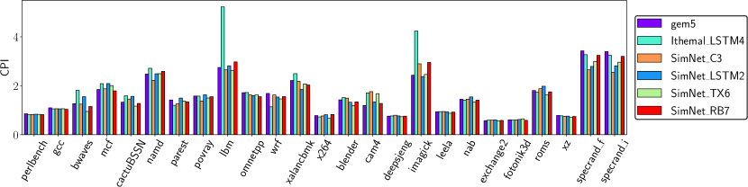
Figure 5. Simulated benchmark CPIs for various approaches.

Benchmark Simulation Accuracy. We conduct simulation experiments on our training platform: the NVIDIA DGX A100 system equipped with eight A100 GPUs and an AMD EPYC 7742 64-core CPU. We simulate all 25 SPEC CPU 2017 SPECrate benchmarks using the reference workload. For each benchmark, SimPoint (Sherwood et al., 2002) is used to select a representative sample of 100 million instructions.

The right side of Table 4 illustrates the simulation errors of various models compared with gem5. We use the absolute value of normalized cycle per instruction (CPI) difference to measure the simulation error for each benchmark: $|CPI_{\text{{SimNet}}}/CPI_{\text{gem5}}-1|\times 100\%$. Although models with lower instruction prediction errors have lower simulation errors in most cases, it is not always true. The reason is because previous prediction results are used to construct the input of latter predictions through the instruction context, which leads to a more complicated relationship between the predictor’s and simulator’s accuracy as will be discussed later.

Table 4 shows the average simulation errors across three benchmark sets: benchmarks used in ML training (i.e., 4 ML benchmarks in Table 3), benchmarks not used in ML training (i.e., 21 simulation benchmarks in Table 3), and all of them. Note that for benchmarks used in training, different input workloads (test vs. reference) and simulation segments (beginning vs. SimPoint selected) are used in their simulation. We observe that the average errors of simulation workloads are not necessarily larger than those of training benchmarks, and the formers are smaller for several models. It demonstrates SimNet’s ability to simulate unseen benchmarks. SimNet’s generalizability roots in the fact that its predictor is trained at the instruction level.

Among SimNet models, the deepest CNN model RB7 achieves the lowest average simulation error of 5.6%. The shallower CNN model C3 also achieves good accuracy with a significantly low computation cost. Therefore, we focus on C3 and RB7 in the following experiments. On the other hand, LSTM and Transformer models achieve comparable simulation accuracy at a cost of one order of magnitude more computation overhead. Compared with Ithemal models, SimNet ones have significantly lower errors, which again demonstrates SimNet’s effectiveness by constructing context explicitly.

Figure 5 further compares the simulated CPIs of gem5, the most accurate Ithemal model LSTM4, and representative SimNet models per benchmark. While Ithemal incurs significant errors for several benchmarks, SimNet models accurately simulates most benchmarks whose CPIs spread across a wide spectrum. Among them, RB7 achieves the best simulation accuracy where only 1 out of 25 benchmarks has an absolute error $>10\%$ (22% for imagick).

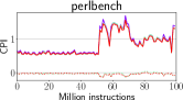
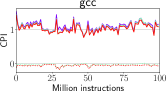
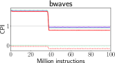
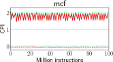
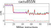
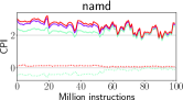
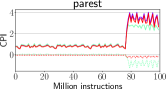
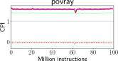
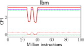
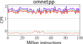
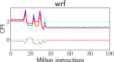
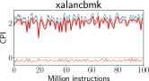
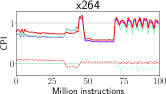
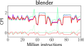
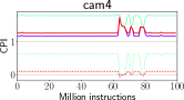
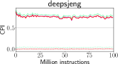
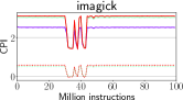
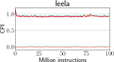
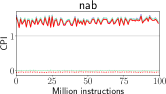
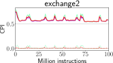
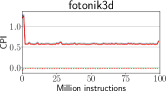
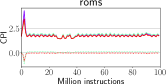
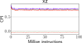
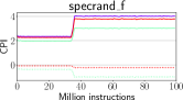
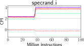
Figure 6. CPI variation during the simulation of 100 million instructions. The solid lines show simulated CPI curves of gem5 and SimNet models. The dotted lines show the simulation errors of SimNet models, calculated by subtracting the CPIs of SimNet models by those of gem5.

Phase Level Accuracy. To verify the simulation accuracy with respect to execution phases, Figure 6 studies the CPI variation under C3 and RB7 models for all 25 benchmarks. Particularly, we calculate the average CPI every 1 million instructions and plot these CPIs over the total simulation length of 100 million instructions. As observed in Figure 6, benchmarks have either steady curves (e.g., povray, leela), high CPI variations (e.g., perlbench, gcc), phased behaviors (e.g., bwaves, specrand), or mixes of them.

For most benchmarks, we observe that SimNet’s CPI curves almost perfectly match those of gem5, especially those using RB7 (i.e., red dotted lines are always close to 0). This phenomenon happens to many highly variable benchmarks such as xalancbmk, which demonstrates SimNet’s ability to capture small CPI variations during simulation. For cam4 where C3 has the largest simulation error (see Figure 5), a consistent error persists across most simulation periods, while RB7 still has a CPI curve that resembles that of gem5. These results show that SimNet not only can predict the overall performance well, but it also generates insights, such as identifying execution phases and performance bottlenecks.

We also observe that a period of inaccurate simulation does not necessarily affect the simulation accuracy of the time periods that follow. For instance, C3’s simulation errors reduce to 0 for 3 short periods when gem5’s CPIs increase for cam4. Another example is cactuBSSN, where C3 fails to simulate it from 20M to 50M accurately, but has an almost identical CPI curve to that of gem5 after 50M.

This observation is counter-intuitive at first glance. Because previous prediction results are used to construct the input of latter predictions through the instruction context, it is reasonable to expect the prediction errors will propagate through the simulation. We discover two reasons behind it. First, the processor pipeline is emptied every once in a while due to events such as branch misprediciton during simulation. Upon these events, there are no context instructions, and the predicted latency does not rely on previous prediction results. As a result, the latency is easier to predict by SimNet models and thus the simulation accuracy gets calibrated on these events. Second, a well-trained SimNet model can self correct its errors throughout the simulation because such self-correction appears in the training data generated from real processors’ behaviors. For example, assume one instruction $I$ takes longer than it should and prevents the next instruction $I_{n}$ from entering the processor earlier. When $I_{n}$ enters, the processor pipeline is emptier than it should be, which results in faster execution of $I_{n}$. In such a scenario, $I$ is executed slower, while $I_{n}$ is executed faster. Together, the total execution time calibrates towards the right direction. These reasons prevent the prediction error from propagating, and thus ensure SimNet’s accuracy during long simulation.

Accuracy Against Hardware. When there is an actual hardware that a simulator intends to simulate, the simulator accuracy can be validated against the hardware. For this purpose, we evaluate the accuracy of SimNet under the gem5 A64FX configuration. The gem5 simulaton of A64FX is verfied to have an average absolute error of 6.6% against the real A64FX processor across a set of benchmarks (Kodama et al., 2019). Since their simulated benchmarks do not include SPEC CPU 2017 benchmarks, we cannot directly calculate the simulation accuracy of SimNet against the A64FX processor. Instead, we deduce the accuracy of SimNet against A64FX as follows. Under a reasonable assumption that the normalized CPI follows a normal/Gaussian distribution, we get the following distributions from SimNet results and (Kodama et al., 2019): $CPI_{\text{{SimNet}}}/CPI_{\text{gem5}}\sim\mathcal{N}(1.062,0.016^{2})$, $CPI_{\text{gem5}}/CPI_{\text{A64FX}}\sim\mathcal{N}(1.013,0.078^{2})$. Their product, $CPI_{\text{{SimNet}}}/CPI_{\text{A64FX}}$, which represents the accuracy of SimNet against A64FX, has a mean of 1.060 and a standard variance of $0.016$ (Smith, 2011). The expected average absoluate simulation error is 6.0% under this distribution, similar to that of gem5.

To give more contexts, a simulator is usually considered to be accurate if simulation errors are around 10%. For example, ZSim reports an average error of 9.7% against an Intel Westmere CPU (Sanchez and Kozyrakis, 2013), and (Gutierrez et al., 2014) reports a 13% error of gem5 against an ARM Cortex-A15 system. Although we cannot directly validate the accuracy of SimNet against A64FX, the deduced average absoluate simulation error is similar to that of gem5 that it learns from. We contend the low simulation error of SimNet is sufficient to gain confidence about its simulation results.

Relative Accuracy. While the simulation accuracy against real hardware is a useful metrics, simulators are often applied in design space exploration where no corresponding hardware exists for verification. In these cases, computer architects care more about the “relative” simulation accuracy, which measures how accurate simulation results reflect the performance variance under certain architecture changes. For instance, how much the performance will improve with doubled cache sizes. Section 5 will demonstrate that SimNet achieves excellent relative accuracies using several case studies.

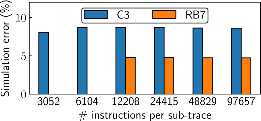
Figure 7. Average parallel simulation errors with various sub-trace sizes.

Figure 8. Simulation throughput with different sub-trace numbers.

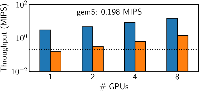
Figure 9. Simulation throughput with multiple GPUs.

4.2. Parallel Simulation

Accuracy. When simulating a single benchmark, because the parallel simulator partitions the input trace into multiple sub-traces, there is simulation accuracy loss across sub-trace boundaries. Figure 9 studies how the overall simulation accuracy varies with the number of instructions per sub-trace. RB7 cannot have sub-traces that are smaller than 12k instructions because the GPU memory cannot accommodate too many sub-traces. As the results show, sub-traces of 3k instructions are sufficient to achieve parallel simulation errors that are similar to sequential ones. The parallel simulation errors vary in a small range with sub-traces of different sizes (around 8% for C3 and 5% for RB7), which demonstrates the reliability of parallel SimNet.

Throughput. We evaluate the simulation throughput of parallel SimNet in terms of million instructions per second (MIPS). Figure 9 evaluates the average throughput across all benchmarks with various numbers of sub-traces using the same models. The x and y axes are on the logarithmic scale. Limited by the GPU memory capacity, we cannot evaluate C3 beyond 32k sub-traces or RB7 beyond 8k sub-traces. We observe that the simulation throughputs improve almost linearly when increasing the number of sub-traces, because more sub-traces allow SimNet to utilize both CPU and GPU resources more efficiently until it saturates them.

Figure 9 assesses the throughput scalability of SimNet with multiple GPUs, where the horizontal black-dotted line marks the gem5 simulation throughput. As ML inferences take a significant portion of time in SimNet, using multiple GPUs improves both the inference and simulation throughputs. Again, SimNet achieves near-linear speedup with the number of GPUs. With eight GPUs, it achieves 15.1 and 1.4 MIPS with the C3 and RB7 models. Correspondingly, this represents $76.2\times$ and $7.4\times$ improvement over gem5. We can further scale SimNet to distributed GPU systems easily for higher throughputs, because very limited communication is involved.

Note that we evaluate the throughput when simulating a single benchmark above. In practical simulation scenarios, computer architects usually need to simulate many benchmarks as well as different configurations. Our design of SimNet can naturally simulate different benchmarks and configurations in parallel, which provides even more opportunities to exploit parallelism.

Comparison with CPU-based Parallel Simulation. Previous CPU-based simulators can make use of multi-core CPUs to simulate multiple programs/threads in parallel (Binkert et al., 2011; Sanchez and Kozyrakis, 2013; Janssen et al., 2010). However, they cannot simulate a single program/thread in parallel and their parallelism is limited by the number of cores (dozens on modern CPUs). In comparison, GPU-based SimNet is able to simulate tens of thousands of traces in parallel on one GPU as shown in Figure 9. These traces can come from a single or multiple programs/threads. As discussed below, such massive parallel simulation of SimNet benefits not only simulation performance, but also power efficiency.

Power Efficiency. GPU-based SimNet can also achieve higher or similar simulation throughputs given a certain power/energy budget compared with traditional CPU-based simulators. On our experimental platform, SimNet has a simulation power efficiency of 4.7 and 0.44 KIPS/watt for C3 and RB7, while that of gem5 is 0.88 KIPS/watt. C3 is the most power efficient model while having acceptable simulation accuracy. While an A100 GPU has a TDP of 400 watts, we expect that SimNet’s power efficiency can be further improved using consumer grade GPUs such as NVIDIA GeForce series or ASIC ML accelerators.

4.3. Overhead Discussion

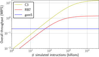
Figure 10. Overall simulation throughput under different instruction numbers.

Training Overhead. Figure 10 shows the overall throughputs of various SimNet models that considers both simulation and training time. It is calculated as $\frac{\text{\# simulated instructions}}{\text{training time}+\text{simulation time}}$. The training overhead amortizes with the increasing number of simulated instructions. The overall throughputs of SimNet exceed that of gem5 by 24 and 59 billion instructions for C3 and RB7, and approach their ideal throughputs with zero training overhead at trillions of instructions. To put it into context, a typical SPEC CPU 2017 benchmark executes more than one trillion instructions using the reference workload, and computer architects typically need to simulate dozens of benchmarks under hundreds of configurations, which means quadrillions of instructions. Even with the help of statistical simulation tools such as SimPoint, simulating trillions of instructions is still needed assuming the common practice of simulating at least 100 million $\sim$ 1 billion instructions per benchmark. The training overhead of SimNet is negligible in these use cases. It is also worth noting that the training and simulation of SimNet can be trivially scaled to large distributed systems, which will further reduce the training overhead.

Functional and History Context Simulation Overhead. Functional simulation can be accomplished using fast instruction set simulators/emulators such as QEMU (Bellard, 2005). History context simulation is also fast because it only requires simplified results, such as cache access levels, where simulating address tag comparison and replacement is sufficient. Our initial experiments and previous research show such simulation can be done at $\sim 100$ MIPS on a single CPU core (Van Dung et al., 2014), which is much larger than SimNet’s simulation throughputs. These overheads are therefore negligible. Further acceleration of functional and history context simulation is possible with GPUs, and we leave it for future works.

4.4. Impact of Features

Figure 11 evaluates the contribution of each input feature to the output for C3 using the SHapley Additive exPlanation (SHAP) method (Lundberg and Lee, 2017). SHAP’s goal is to explain the prediction of an instance by computing the contribution of each feature to the prediction. It computes Shapley values (Shapley, 1953) using the coalitional game theory. Shapley value is the average marginal contribution of a feature value across all possible coalitions. We take the average of absolute Shapley values on training samples for each feature to produce feature attribution scores. Figure 11a and 11b summarize the attribution scores of to-be-predicted instructions and context instructions separately. We categorize the 50 features into latency, operation, register, and memory. Memory and operation features generally have more impacts on the prediction results. The most influential feature of to-be-predicted instructions is the fetch access level because the fetch latency depends on it. For context instructions, the branch misprediction flag has the largest attribution score as mispredicted branches need to flush the processor pipeline.

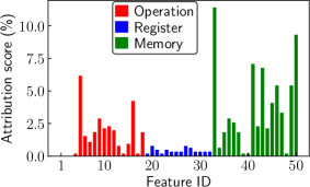
(a) To-be-predicted instruction.

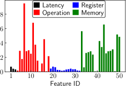
(b) Context instructions.

Figure 11. Feature attribution scores.

4.5. Impact of Training Dataset Size

We also generate a large ML training dataset using 15 SPEC CPU 2017 benchmarks instead of four. Our results show that using the large dataset reduces the average simulation error by 33% at a cost of $3\times$ training time. While larger training datasets further improve accuracy, we conclude that the smaller dataset is enough to train accurate models and also requires less training time.

The reason why a small training dataset is sufficient is because most benchmarks use a variety of instructions which provide ample samples to train the instruction latency predictor. We expect reasonable ML prediction accuracy as long as there are adequate samples to cover enough instruction and context scenarios, and the results show that 4 benchmarks are enough to obtain sufficient scenarios. Benchmark selection for the training set is also not critical.

5. Use Scenarios

SimNet can be applied in many computer architecture research and engineering scenarios. First, many recent computer architecture efforts focus on caches or branch predictors while other microarchitecture components are more sophisticated and less likely to be subjects of change. In such scenarios, pre-trained SimNet models can be directly applied as caches and branch predictors are modeled in history context simulation, and no additional training is required (i.e., the training overhead discussed in Section 4.3 does not exist.). Second, when studying other microarchitecture parameters (e.g., ROB size) or novel components, different parameter/configuration choices can be included in the input of the model, so training a single model is sufficient to study all variations. We illustrate both use scenarios below, where the first two cases do not require training, and the last case requires a one time training.

	Simulated speedup			Relative error range
	gem5	C3	RB7	C3	RB7
BiMode_l	10.4%	11.2%	9.9%	[-2.7%, 3.7%]	[-1.7%, 1.4%]
TAGE-SC-L	12.3%	13.7%	12.4%	[-4.0%, 4.5%]	[-0.7%, 1.8%]

Table 5. Simulated speedups of various branch predictors.

Branch Predictor Study. We compare the simulated performance of two branch predictors using gem5 and SimNet, including a large bi-mode branch predictor (BiMode_l) and the recently proposed TAGE-SC-L (Seznec, 2016). Their implementation in gem5 is used in SimNet’s history context simulation to generate branch misprediction flags for ML models’ input. Table 5 shows the simulated average speedups across SPEC benchmarks, where the speedup is calculated against the performance of a baseline bi-mode branch predictor. We observe that the average speedups obtained using SimNet are similar to those using gem5. Moreover, the right side of Table 5 shows the speedup error ranges of individual benchmarks compared with gem5 results. We observe that SimNet also predicts the speedups of individual benchmarks well, especially under RB7.

L2 Cache Size Exploration. We also simulate the performance impact of L2 cache sizes using gem5 and SimNet. Similar to the branch predictor case, SimNet accurately simulates the relative speedup under cache sizes from 256 kB to 4 MB, and the average error against gem5 is 0.8%.

ROB Size Exploration. In this experiment, the ML model input includes the ROB size as an additional feature to account for its impact. The training data are generated by running the same four SPEC benchmarks in gem5 under various ROB sizes. We train a C3 model to study the impact of ROB sizes. Again, the simulation results of SimNet and gem5 agree with each other. For example, the average performance improvement when increasing the number of ROB entries from 40 to 80 and 120 is 1.2% and 1.4% under gem5. Using SimNet, the corresponding speedups are 1.1% and 1.5%, which are very similar.

6. Related Work

ML for Latency Prediction. Ithemal (Mendis et al., 2019) uses LSTM models to predict the execution latency of static basic blocks. The instructions within a block are fed into the model in the form of assembly, such as words in NLP. On top of Ithemal, DiffTune (Renda et al., 2020) trains a differentiable ML performance model to configure the simulator parameters to closely resemble a target architecture. These methods pose limits as they do not consider dynamic execution behaviors, such as memory accesses and branches, which have significant impacts on program performance. They also target basic blocks with a limited number of instructions. As a result, they are not applicable to a computer architecture simulator that needs to simulate realistic processors and billions/trillions of instructions.

ML for Application Performance Prediction. Ipek et al. propose using neural networks for application performance prediction (Ïpek et al., 2006). Meanwhile, Lee et al. formulate nonlinear regression models for performance and power prediction (Lee and Brooks, 2007; Lee et al., 2007). Eyerman et al. propose inferring unknown parameters of mechanistic performance models using regression, to balance between model accuracy and interpretability (Eyerman et al., 2011). Mosmodel (Agbarya et al., 2020) is a multi-input polynomial model used for virtual memory research that can predict the program execution time given the page table walking statistics. Wu et al. use performance counters as the input of ML models to predict GPU performance and power (Wu et al., 2015). Nemirovsky et al. schedule threads based on ML-based performance models (Nemirovsky et al., 2017). Some approaches are proposed to predict a processor’s performance/power based on those obtained on different types of processors (Ardalani et al., 2015; Baldini et al., 2014; O’neal et al., 2017) or with different ISAs (Zheng et al., 2015, 2016).

While these works build performance models on a per-program/input basis, SimNet works at the instruction level. Therefore, these application-centric approaches require generating training data and retraining models when target applications change, and the overhead of doing so is significant. On the other hand, SimNet can directly simulate any application, making it much more flexible.

ML for Other Architecture Research. In addition to the aforementioned uses, ML has been widely applied to many other computer architecture aspects, including microarchitecture design and energy/power optimization. These applications are summarized in (Penney and Chen, 2019; Wu and Xie, 2021).

Simulation with Statistical Sampling. Instead of simulating the entire program, statistical simulation selectively simulates representative sampling units and infers the overall performance from these sample simulation results statistically (Conte et al., 1996). SMARTS (Wunderlich et al., 2003; Wenisch et al., 2006) periodically switches between detailed and functional simulation to obtain an accurate CPI estimation with minimal detailed simulation.

SimPoint records the basic block execution frequencies of individual sampling units and those of the whole program to select representative ones with the aim that the selected samples capture the overall execution behaviors well (Sherwood et al., 2002; Perelman et al., 2003). Similarly, PinPoints uses dynamic binary instrumentation to find representative samples for X86 programs (Patil et al., 2004), and BarrierPoint applies sampling to multi-threaded simulation (Carlson et al., 2014). These methods require pre-analyzing the simulated program with a certain input, while our ML-based simulator can be applied directly to any program and input combination because of its instruction-centric approach.

One key challenge in statistical simulation is to keep track of the microarchitecture state between detailed simulation fractions, especially cache states. To simulate the cache behavior accurately in statistical simulation, Nikoleris et al. propose using Linux KVM to monitor the reuse distance of selected cache lines (Nikoleris et al., 2019). Similarly, Sandberg et al. leverage hardware virtualization to fast-forward between samples, so different samples can be simulated in parallel (Sandberg et al., 2015). These statistical simulation approaches can be used together with SimNet to further accelerate the detailed simulation portions. As an example, Section 4 uses SimPoint and SimNet together.

Traditional Simulation Acceleration. ZSim is an X86 simulator that supports many-core system simulation (Sanchez and Kozyrakis, 2013). It decouples the simulation of individual cores and resources shared across cores, as well as adopts a simplified core model. As a result, it achieves $\sim 10$ MIPS for single-thread workload simulation on an Intel Sandy Bridge 16-core processor. SST (Janssen et al., 2010) distributes the simulation of different components across Message Passing Interface (MPI) ranks to achieve parallel simulation. Field programmable gate array (FPGA)-based emulators run significantly faster than simulation software but require a huge amount of effort to develop and validate register-transfer level models (Karandikar et al., 2018). In comparison, our work accelerates simulation from a different angle to make the most of widely available ML accelerators, such as GPUs.

7. Conclusions

This work proposes a new computer architecture simulation paradigm using ML. To the best of our knowledge, this effort is the first to demonstrate ML’s applicability to full-fledged architecture simulation. This new methodology significantly improves simulation performance without sacrificing accuracy. In addition to discrete-event, analytical, or other statistical approaches to architectural simulation/modeling, we maintain this new class of simulators will become a useful, valuable addition to the architect’s “bag-of-tools.” We recognize several advantages of this new approach.

1) We demonstrate that ML-based simulators can predict overall performance accurately, and they also qualitatively capture architecture and application behaviors. 2) ML is intrinsically easier to parallelize than discrete-event simulation. Moreover, ML-based simulators capitalize on modern computing technology that is tailored for boosting ML performance. 3) ML-based simulators generalize well to a large spectrum of application workloads. In our approach, this stems from building them around an instruction-level latency predictor. Hence, the focus is on learning instruction behaviors rather than high-level program behaviors that are much more difficult to capture. 4) The training data are easy and fast to obtain. Potential sources of training data are multiple, including simplified models of simulators, actual execution of code on existing systems, or historical performance data.

Future Directions. We plan to investigate ML-based approaches that support multi-thread/program simulation as our next step. The key to supporting multi-thread/program simulation is to model communications. We describe two possible strategies as follows, 1) extending context instructions to include concurrently executed instructions from other threads/programs, and 2) training ML models to model the impact of shared resources (e.g., caches, memory).

- (1)
- dgx (2020) 2020. DGX A100: Universal System for AI Infrastructure. https://www.nvidia.com/en-us/data-center/dgx-a100/
- Abadi et al. (2016) Martín Abadi, Paul Barham, Jianmin Chen, Zhifeng Chen, Andy Davis, Jeffrey Dean, Matthieu Devin, Sanjay Ghemawat, Geoffrey Irving, Michael Isard, et al. 2016. Tensorflow: A system for large-scale machine learning. In 12th USENIX symposium on operating systems design and implementation (OSDI 16). 265–283.
- Agbarya et al. (2020) Mohammad Agbarya, Idan Yaniv, Jayneel Gandhi, and Dan Tsafrir. 2020. Predicting execution times with partial simulations in virtual memory research: why and how. In IEEE/ACM International Symposium on Microarchitecture (MICRO). Global Online Event. (to appear).
- Ardalani et al. (2015) Newsha Ardalani, Clint Lestourgeon, Karthikeyan Sankaralingam, and Xiaojin Zhu. 2015. Cross-Architecture Performance Prediction (XAPP) Using CPU Code to Predict GPU Performance. In Proceedings of the 48th International Symposium on Microarchitecture (Waikiki, Hawaii) (MICRO-48). Association for Computing Machinery, New York, NY, USA, 725–737. https://doi.org/10.1145/2830772.2830780
- Baldini et al. (2014) I. Baldini, S. J. Fink, and E. Altman. 2014. Predicting GPU Performance from CPU Runs Using Machine Learning. In 2014 IEEE 26th International Symposium on Computer Architecture and High Performance Computing. 254–261. https://doi.org/10.1109/SBAC-PAD.2014.30
- Bellard (2005) Fabrice Bellard. 2005. QEMU, a fast and portable dynamic translator.. In USENIX annual technical conference, FREENIX Track, Vol. 41. Califor-nia, USA, 46.
- Binkert et al. (2011) Nathan Binkert, Bradford Beckmann, Gabriel Black, Steven K. Reinhardt, Ali Saidi, Arkaprava Basu, Joel Hestness, Derek R. Hower, Tushar Krishna, Somayeh Sardashti, and et al. 2011. The Gem5 Simulator. SIGARCH Comput. Archit. News 39, 2 (Aug. 2011), 1–7. https://doi.org/10.1145/2024716.2024718
- Bucek et al. (2018) James Bucek, Klaus-Dieter Lange, and Jóakim v. Kistowski. 2018. SPEC CPU2017: Next-generation compute benchmark. In Companion of the 2018 ACM/SPEC International Conference on Performance Engineering. 41–42.
- Carlson et al. (2014) T. E. Carlson, W. Heirman, K. Van Craeynest, and L. Eeckhout. 2014. BarrierPoint: Sampled simulation of multi-threaded applications. In 2014 IEEE International Symposium on Performance Analysis of Systems and Software (ISPASS). 2–12. https://doi.org/10.1109/ISPASS.2014.6844456
- Conte et al. (1996) T. M. Conte, M. A. Hirsch, and K. N. Menezes. 1996. Reducing state loss for effective trace sampling of superscalar processors. In Proceedings International Conference on Computer Design. VLSI in Computers and Processors. 468–477. https://doi.org/10.1109/ICCD.1996.563595
- Elsken et al. (2019) Thomas Elsken, Jan Hendrik Metzen, and Frank Hutter. 2019. Neural architecture search: A survey. The Journal of Machine Learning Research 20, 1 (2019), 1997–2017.
- Eyerman et al. (2011) Stijn Eyerman, Kenneth Hoste, and Lieven Eeckhout. 2011. Mechanistic-empirical processor performance modeling for constructing CPI stacks on real hardware. In (IEEE ISPASS) IEEE International Symposium on Performance Analysis of Systems and Software. 216–226. https://doi.org/10.1109/ISPASS.2011.5762738
- Gutierrez et al. (2014) A. Gutierrez, J. Pusdesris, R. G. Dreslinski, T. Mudge, C. Sudanthi, C. D. Emmons, M. Hayenga, and N. Paver. 2014. Sources of error in full-system simulation. In 2014 IEEE International Symposium on Performance Analysis of Systems and Software (ISPASS). 13–22. https://doi.org/10.1109/ISPASS.2014.6844457
- He et al. (2016) Kaiming He, Xiangyu Zhang, Shaoqing Ren, and Jian Sun. 2016. Deep residual learning for image recognition. In Proceedings of the IEEE conference on computer vision and pattern recognition. 770–778.
- Hochreiter and Schmidhuber (1997) Sepp Hochreiter and Jürgen Schmidhuber. 1997. Long short-term memory. Neural computation 9, 8 (1997), 1735–1780.
- Ïpek et al. (2006) Engin Ïpek, Sally A. McKee, Rich Caruana, Bronis R. de Supinski, and Martin Schulz. 2006. Efficiently Exploring Architectural Design Spaces via Predictive Modeling. In Proceedings of the 12th International Conference on Architectural Support for Programming Languages and Operating Systems (San Jose, California, USA) (ASPLOS XII). Association for Computing Machinery, New York, NY, USA, 195–206. https://doi.org/10.1145/1168857.1168882
- Jaleel et al. (2008) Aamer Jaleel, Robert S Cohn, Chi-Keung Luk, and Bruce Jacob. 2008. CMP$im: A Pin-based on-the-fly multi-core cache simulator. In Proceedings of the Fourth Annual Workshop on Modeling, Benchmarking and Simulation (MoBS), co-located with ISCA. 28–36.
- Janssen et al. (2010) Curtis L Janssen, Helgi Adalsteinsson, Scott Cranford, Joseph P Kenny, Ali Pinar, David A Evensky, and Jackson Mayo. 2010. A simulator for large-scale parallel computer architectures. International Journal of Distributed Systems and Technologies (IJDST) 1, 2 (2010), 57–73.
- Jia et al. (2020) Weile Jia, Han Wang, Mohan Chen, Denghui Lu, Lin Lin, Roberto Car, Weinan E, and Linfeng Zhang. 2020. Pushing the Limit of Molecular Dynamics with Ab Initio Accuracy to 100 Million Atoms with Machine Learning. In Proceedings of the International Conference for High Performance Computing, Networking, Storage and Analysis (Atlanta, Georgia) (SC ’20). IEEE Press, Article 5, 14 pages.
- Jouppi et al. (2017) Norman P. Jouppi, Cliff Young, Nishant Patil, David Patterson, Gaurav Agrawal, Raminder Bajwa, Sarah Bates, Suresh Bhatia, Nan Boden, Al Borchers, Rick Boyle, Pierre-luc Cantin, Clifford Chao, Chris Clark, Jeremy Coriell, Mike Daley, Matt Dau, Jeffrey Dean, Ben Gelb, Tara Vazir Ghaemmaghami, Rajendra Gottipati, William Gulland, Robert Hagmann, C. Richard Ho, Doug Hogberg, John Hu, Robert Hundt, Dan Hurt, Julian Ibarz, Aaron Jaffey, Alek Jaworski, Alexander Kaplan, Harshit Khaitan, Daniel Killebrew, Andy Koch, Naveen Kumar, Steve Lacy, James Laudon, James Law, Diemthu Le, Chris Leary, Zhuyuan Liu, Kyle Lucke, Alan Lundin, Gordon MacKean, Adriana Maggiore, Maire Mahony, Kieran Miller, Rahul Nagarajan, Ravi Narayanaswami, Ray Ni, Kathy Nix, Thomas Norrie, Mark Omernick, Narayana Penukonda, Andy Phelps, Jonathan Ross, Matt Ross, Amir Salek, Emad Samadiani, Chris Severn, Gregory Sizikov, Matthew Snelham, Jed Souter, Dan Steinberg, Andy Swing, Mercedes Tan, Gregory Thorson, Bo Tian, Horia Toma, Erick Tuttle, Vijay Vasudevan, Richard Walter, Walter Wang, Eric Wilcox, and Doe Hyun Yoon. 2017. In-Datacenter Performance Analysis of a Tensor Processing Unit. In Proceedings of the 44th Annual International Symposium on Computer Architecture (Toronto, ON, Canada) (ISCA ’17). Association for Computing Machinery, New York, NY, USA, 1–12. https://doi.org/10.1145/3079856.3080246
- Karandikar et al. (2018) Sagar Karandikar, Howard Mao, Donggyu Kim, David Biancolin, Alon Amid, Dayeol Lee, Nathan Pemberton, Emmanuel Amaro, Colin Schmidt, Aditya Chopra, Qijing Huang, Kyle Kovacs, Borivoje Nikolic, Randy Katz, Jonathan Bachrach, and Krste Asanović. 2018. Firesim: FPGA-Accelerated Cycle-Exact Scale-out System Simulation in the Public Cloud. In Proceedings of the 45th Annual International Symposium on Computer Architecture (Los Angeles, California) (ISCA ’18). IEEE Press, 29–42. https://doi.org/10.1109/ISCA.2018.00014
- Kingma and Ba (2015) P. Diederik Kingma and Lei Jimmy Ba. 2015. Adam: A Method for Stochastic Optimization. international conference on learning representations (2015).
- Kodama et al. (2019) Yuetsu Kodama, Tetsuya Odajima, Akira Asato, and Mitsuhisa Sato. 2019. Evaluation of the riken post-k processor simulator. arXiv preprint arXiv:1904.06451 (2019).
- Krizhevsky et al. (2012) Alex Krizhevsky, Ilya Sutskever, and Geoffrey E Hinton. 2012. Imagenet classification with deep convolutional neural networks. Advances in neural information processing systems 25 (2012), 1097–1105.
- Lee and Brooks (2007) B. C. Lee and D. M. Brooks. 2007. Illustrative Design Space Studies with Microarchitectural Regression Models. In 2007 IEEE 13th International Symposium on High Performance Computer Architecture. 340–351. https://doi.org/10.1109/HPCA.2007.346211
- Lee et al. (2007) Benjamin C. Lee, David M. Brooks, Bronis R. de Supinski, Martin Schulz, Karan Singh, and Sally A. McKee. 2007. Methods of Inference and Learning for Performance Modeling of Parallel Applications. In Proceedings of the 12th ACM SIGPLAN Symposium on Principles and Practice of Parallel Programming (San Jose, California, USA) (PPoPP ’07). Association for Computing Machinery, New York, NY, USA, 249–258. https://doi.org/10.1145/1229428.1229479
- Lundberg and Lee (2017) Scott M Lundberg and Su-In Lee. 2017. A Unified Approach to Interpreting Model Predictions. In Advances in Neural Information Processing Systems 30, I. Guyon, U. V. Luxburg, S. Bengio, H. Wallach, R. Fergus, S. Vishwanathan, and R. Garnett (Eds.). Curran Associates, Inc., 4765–4774.
- Mendis et al. (2019) Charith Mendis, Alex Renda, Saman Amarasinghe, and Michael Carbin. 2019. Ithemal: Accurate, portable and fast basic block throughput estimation using deep neural networks. In International Conference on Machine Learning. PMLR, 4505–4515.
- Nemirovsky et al. (2017) Daniel Nemirovsky, Tugberk Arkose, Nikola Markovic, Mario Nemirovsky, Osman Unsal, and Adrian Cristal. 2017. A Machine Learning Approach for Performance Prediction and Scheduling on Heterogeneous CPUs. In 2017 29th International Symposium on Computer Architecture and High Performance Computing (SBAC-PAD). 121–128. https://doi.org/10.1109/SBAC-PAD.2017.23
- Nikoleris et al. (2019) Nikos Nikoleris, Lieven Eeckhout, Erik Hagersten, and Trevor E. Carlson. 2019. Directed Statistical Warming through Time Traveling. In Proceedings of the 52nd Annual IEEE/ACM International Symposium on Microarchitecture (Columbus, OH, USA) (MICRO ’52). Association for Computing Machinery, New York, NY, USA, 1037–1049. https://doi.org/10.1145/3352460.3358264
- O’neal et al. (2017) Kenneth O’neal, Philip Brisk, Ahmed Abousamra, Zack Waters, and Emily Shriver. 2017. GPU Performance Estimation Using Software Rasterization and Machine Learning. ACM Trans. Embed. Comput. Syst. 16, 5s, Article 148 (Sept. 2017), 21 pages. https://doi.org/10.1145/3126557
- Paszke et al. (2019) Adam Paszke, Sam Gross, Francisco Massa, Adam Lerer, James Bradbury, Gregory Chanan, Trevor Killeen, Zeming Lin, Natalia Gimelshein, Luca Antiga, Alban Desmaison, Andreas Kopf, Edward Yang, Zachary DeVito, Martin Raison, Alykhan Tejani, Sasank Chilamkurthy, Benoit Steiner, Lu Fang, Junjie Bai, and Soumith Chintala. 2019. PyTorch: An Imperative Style, High-Performance Deep Learning Library. In Advances in Neural Information Processing Systems, H. Wallach, H. Larochelle, A. Beygelzimer, F. d'Alché-Buc, E. Fox, and R. Garnett (Eds.), Vol. 32. Curran Associates, Inc., 8026–8037. https://proceedings.neurips.cc/paper/2019/file/bdbca288fee7f92f2bfa9f7012727740-Paper.pdf
- Patel et al. (2011) A. Patel, F. Afram, S. Chen, and K. Ghose. 2011. MARSS: A full system simulator for multicore x86 CPUs. In 2011 48th ACM/EDAC/IEEE Design Automation Conference (DAC). 1050–1055.
- Patil et al. (2004) H. Patil, R. Cohn, M. Charney, R. Kapoor, A. Sun, and A. Karunanidhi. 2004. Pinpointing Representative Portions of Large Intel ® Itanium ® Programs with Dynamic Instrumentation. In 37th International Symposium on Microarchitecture (MICRO-37’04). 81–92. https://doi.org/10.1109/MICRO.2004.28
- Penney and Chen (2019) Drew D Penney and Lizhong Chen. 2019. A survey of machine learning applied to computer architecture design. arXiv preprint arXiv:1909.12373 (2019).
- Perelman et al. (2003) Erez Perelman, Greg Hamerly, Michael Van Biesbrouck, Timothy Sherwood, and Brad Calder. 2003. Using SimPoint for Accurate and Efficient Simulation. SIGMETRICS Perform. Eval. Rev. 31, 1 (June 2003), 318–319.
- Renda et al. (2020) Alex Renda, Yishen Chen, Charith Mendis, and Michael Carbin. 2020. DiffTune: Optimizing CPU Simulator Parameters with Learned Differentiable Surrogates. In IEEE/ACM International Symposium on Microarchitecture.
- Rumelhart et al. (1986) David E Rumelhart, Geoffrey E Hinton, and Ronald J Williams. 1986. Learning representations by back-propagating errors. nature 323, 6088 (1986), 533–536.
- Sanchez and Kozyrakis (2013) Daniel Sanchez and Christos Kozyrakis. 2013. ZSim: Fast and Accurate Microarchitectural Simulation of Thousand-Core Systems. SIGARCH Comput. Archit. News 41, 3 (June 2013), 475–486. https://doi.org/10.1145/2508148.2485963
- Sandberg et al. (2015) A. Sandberg, N. Nikoleris, T. E. Carlson, E. Hagersten, S. Kaxiras, and D. Black-Schaffer. 2015. Full Speed Ahead: Detailed Architectural Simulation at Near-Native Speed. In 2015 IEEE International Symposium on Workload Characterization. 183–192. https://doi.org/10.1109/IISWC.2015.29
- Sato et al. (2020) M. Sato, Y. Ishikawa, H. Tomita, Y. Kodama, T. Odajima, M. Tsuji, H. Yashiro, M. Aoki, N. Shida, I. Miyoshi, K. Hirai, A. Furuya, A. Asato, K. Morita, and T. Shimizu. 2020. Co-Design for A64FX Manycore Processor and ”Fugaku”. In SC20: International Conference for High Performance Computing, Networking, Storage and Analysis. 1–15. https://doi.org/10.1109/SC41405.2020.00051
- Senior et al. (2020) Andrew W Senior, Richard Evans, John Jumper, James Kirkpatrick, Laurent Sifre, Tim Green, Chongli Qin, Augustin Žídek, Alexander WR Nelson, Alex Bridgland, et al. 2020. Improved protein structure prediction using potentials from deep learning. Nature 577, 7792 (2020), 706–710.
- Seznec (2016) André Seznec. 2016. TAGE-SC-L Branch Predictors Again. In 5th JILP Workshop on Computer Architecture Competitions (JWAC-5): Championship Branch Prediction (CBP-5). Seoul, South Korea. https://hal.inria.fr/hal-01354253
- Shapley (1953) Lloyd S Shapley. 1953. A value for n-person games. Contributions to the Theory of Games 2, 28 (1953), 307–317.
- Sherwood et al. (2002) Timothy Sherwood, Erez Perelman, Greg Hamerly, and Brad Calder. 2002. Automatically Characterizing Large Scale Program Behavior. In Proceedings of the 10th International Conference on Architectural Support for Programming Languages and Operating Systems (San Jose, California) (ASPLOS X). Association for Computing Machinery, New York, NY, USA, 45–57. https://doi.org/10.1145/605397.605403
- Smith (2011) Julius O. Smith. 2011. Spectral Audio Signal Processing. https://ccrma.stanford.edu/~jos/sasp online book, 2011 edition.
- Tan et al. (2019) Mingxing Tan, Bo Chen, Ruoming Pang, Vijay Vasudevan, Mark Sandler, Andrew Howard, and Quoc V. Le. 2019. MnasNet: Platform-Aware Neural Architecture Search for Mobile. In Proceedings of the IEEE/CVF Conference on Computer Vision and Pattern Recognition (CVPR).
- Tan and Le (2019) Mingxing Tan and Quoc Le. 2019. EfficientNet: Rethinking Model Scaling for Convolutional Neural Networks. In Proceedings of the 36th International Conference on Machine Learning (Proceedings of Machine Learning Research, Vol. 97), Kamalika Chaudhuri and Ruslan Salakhutdinov (Eds.). PMLR, 6105–6114. http://proceedings.mlr.press/v97/tan19a.html
- Van Dung et al. (2014) Tran Van Dung, Ittetsu Taniguchi, and Hiroyuki Tomiyama. 2014. Cache Simulation for Instruction Set Simulator QEMU. In 2014 IEEE 12th International Conference on Dependable, Autonomic and Secure Computing. 441–446. https://doi.org/10.1109/DASC.2014.85
- Vanholder (2016) Han Vanholder. 2016. Efficient inference with tensorrt.
- Vaswani et al. (2017) Ashish Vaswani, Noam Shazeer, Niki Parmar, Jakob Uszkoreit, Llion Jones, Aidan N Gomez, Łukasz Kaiser, and Illia Polosukhin. 2017. Attention is all you need. In Advances in neural information processing systems. 5998–6008.
- Wenisch et al. (2006) T. F. Wenisch, R. E. Wunderlich, M. Ferdman, A. Ailamaki, B. Falsafi, and J. C. Hoe. 2006. SimFlex: Statistical Sampling of Computer System Simulation. IEEE Micro 26, 4 (2006), 18–31. https://doi.org/10.1109/MM.2006.79
- Wu et al. (2015) Gene Wu, Joseph L. Greathouse, Alexander Lyashevsky, Nuwan Jayasena, and Derek Chiou. 2015. GPGPU performance and power estimation using machine learning. In 2015 IEEE 21st International Symposium on High Performance Computer Architecture (HPCA). 564–576. https://doi.org/10.1109/HPCA.2015.7056063
- Wu and Xie (2021) Nan Wu and Yuan Xie. 2021. A Survey of Machine Learning for Computer Architecture and Systems. arXiv preprint arXiv:2102.07952 (2021).
- Wunderlich et al. (2003) Roland E. Wunderlich, Thomas F. Wenisch, Babak Falsafi, and James C. Hoe. 2003. SMARTS: Accelerating Microarchitecture Simulation via Rigorous Statistical Sampling. In Proceedings of the 30th Annual International Symposium on Computer Architecture (San Diego, California) (ISCA ’03). Association for Computing Machinery, New York, NY, USA, 84–97. https://doi.org/10.1145/859618.859629
- Yoshida (2018) Toshio Yoshida. 2018. Fujitsu high performance CPU for the Post-K Computer. In Hot Chips, Vol. 30.
- Zheng et al. (2016) Xinnian Zheng, Lizy K. John, and Andreas Gerstlauer. 2016. Accurate Phase-Level Cross-Platform Power and Performance Estimation. In Proceedings of the 53rd Annual Design Automation Conference (Austin, Texas) (DAC ’16). Association for Computing Machinery, New York, NY, USA, Article 4, 6 pages. https://doi.org/10.1145/2897937.2897977
- Zheng et al. (2015) Xinnian Zheng, Pradeep Ravikumar, Lizy K John, and Andreas Gerstlauer. 2015. Learning-based analytical cross-platform performance prediction. In 2015 International Conference on Embedded Computer Systems: Architectures, Modeling, and Simulation (SAMOS). IEEE, 52–59.