Dynamical scaling of Loschmidt echo in non-Hermitian systems

Abstract

We show that non-Hermitian biorthogonal many-body phase transitions can be characterized by the enhanced decay of Loschmidt echo. The quantum criticality is numerically investigated in a non-Hermitian transverse field Ising model by performing the finite-size dynamical scaling of Loschmidt echo. We determine the equilibrium correlation length critical exponents that are consistent with previous results from the exact diagonalization. More importantly, we introduce a simple method to detect quantum phase transitions with the short-time average of rate function motivated by the critically enhanced decay behavior of Loschmidt echo. Our studies show how to detect equilibrium many-body phase transitions with biorthogonal Loschmidt echo that can be observed in future experiments via quantum dynamics after a quench.

Introduction.- The research on quantum phase transitions is one of the central issues in condensed matter physics Sachdev (1999). One goal of current research is to discover novel quantum matters and quantum phase transitions Levin and Wen (2006). Recently, an active research field is to investigate interesting quantum phases and quantum phase transitions in non-Hermitian systems. Previous studies show that non-Hermitian systems can exhibit a lot of fascinating phenomena without counterpart in Hermitian systems Bergholtz et al. (2021); Ashida et al. (2021), such as the bulk-boundary correspondence breakdown and the non-Hermitian skin effect Lee (2016); Yao and Wang (2018); Kunst et al. (2018); Xiong (2018); Gong et al. (2018); Martinez Alvarez et al. (2018); Yokomizo and Murakami (2019); Okuma et al. (2020); Zhang et al. (2020a); Yang et al. (2020a); Wang et al. (2020a); Jiang et al. (2020); Weidemann et al. (2020); Xiao et al. (2020); Borgnia et al. (2020), exceptional points and the bulk Fermi arcs Heiss (2012); Kozii and Fu (2017); Hodaei et al. (2017); Zhou et al. (2018a); Miri and Alu (2019); Park et al. (2019); Yang and Hu (2019); Özdemir et al. (2019); Dóra et al. (2019); Jin et al. (2020); Xiao et al. (2021). The extension to non-Hermitian interacting many-body systems are also explored to understand the effect of non-Hermiticity Matsumoto et al. (2020); Yang et al. (2020b); Ashida et al. (2017); Chang et al. (2020); Lee et al. (2020); Pan et al. (2020a, b); Xu and Chen (2020); Zhang et al. (2020b); Lee (2021); Shackleton and Scheurer (2020); Liu et al. (2020); Yang et al. (2021); Herviou et al. (2019); Yoshida et al. (2019, 2020). It is shown that new types of phase transitions can occur between gapped phases without gap closing in non-Hermitian many-body models Matsumoto et al. (2020); Yang et al. (2020b). Consequently, a key issue is to find the phase transition and figure out the nature of the quantum criticality.

In Hermitian systems, a second-order phase transition can be described by a phenomenological order parameter according to the Landau-Ginzburg theory. Hence, a Hermitian system usually undergoes a phase transition with the gap closing from an ordered phase with a nonzero order parameter to a disordered phase with a vanishing order parameter. Thanks to the development of quantum information science, quantum phase transitions and critical phenomena can also be understood with the concepts from quantum information, i.e. the quantum entanglement Osterloh et al. (2002); Horodecki et al. (2009); Eisert et al. (2010), the quantum fidelity Zanardi and Paunković (2006); You et al. (2007); Campos Venuti and Zanardi (2007); Gu (2010); Albuquerque et al. (2010); Sun (2017); Zhu et al. (2018); Wei and Lv (2018); Chen et al. (2008); Gu et al. (2008); Yang et al. (2008); Luo et al. (2018); Sun et al. (2015) and the Loschmidt echo (LE) Quan et al. (2006); Hwang et al. (2019); Mukherjee et al. (2012); Karl et al. (2017); Pelissetto et al. (2018); Nigro et al. (2019); Titum et al. (2019); Halimeh et al. (2021); Dağ and Sun (2021); Rossini and Vicari (2021). A natural question is whether such approaches can also be used to characterize the non-Hermitian many-body phase transitions.

Recently, above approaches were extended to non-Hermitian systems to identify phase transitions Chang et al. (2020); Herviou et al. (2019); Sun et al. (2022); Tzeng et al. (2021); Solnyshkov et al. (2021); Zhang and Song (2021); Pará et al. (2021); Xu and Chen (2021); Zhou et al. (2018b); Zhou and Du (2021); Zhai and Yin (2020). Here, we are interested in non-Hermitian many-body systems with real eigenvalues whereby we can define the ground state, and focus on the LE that can be realized in experiments via a quench dynamics Xiao et al. (2020); Qiu et al. (2019); Wang et al. (2019). The LE is defined as the overlap between an initial ground-state and its time-evolved state, which exhibits a decay and revival behavior influenced by the quantum criticality Quan et al. (2006); Hwang et al. (2019).

In this paper, we study the dynamical scaling laws of biorthogonal LE in close proximity to the critical point of one-dimensional non-Hermitian transverse field Ising model. We perform the finite-size scaling theory and demonstrate that the system undergoes a second-order phase transition with the Ising universal class by numerically determining the equilibrium correlation length critical exponents of the model. What is more, we introduce the time average of rate function to illustrate how to study the quantum criticality without knowing the critical value or even without assuming the phase transition existence in advance. Consequently, the biorthogonal LE can serve as a simple probe of discovering the non-Hermitian many-body phase transitions due to the critically enhanced decay behavior.

Biorthogonal Loschmidt echo.- Given a general non-Hermitian system that is described by the Hamiltonian,

$$H(\lambda)=H_{0}+\lambda H_{1},$$ (1)

with a control parameter $\lambda$, and the $H(\lambda)\neq H^{\dagger}(\lambda)$. The time-independent Schrödinger equations for the $H(\lambda)$ and $H^{{\dagger}}(\lambda)$ can be written as, Sun et al. (2022); Brody (2013); Sternheim and Walker (1972)

$$H(\lambda)|\psi_{j}^{R}(\lambda)\rangle=E_{j}(\lambda)|\psi_{j}^{R}(\lambda)\rangle,$$ (2)

$$H^{{\dagger}}(\lambda)|\psi_{j}^{L}(\lambda)\rangle=E_{j}^{\ast}(\lambda)|\psi_{j}^{L}(\lambda)\rangle,$$ (3)

where the $E_{j}(\lambda)$, $E_{j}^{\ast}(\lambda)$ and the $|\psi_{j}^{R}(\lambda)\rangle$, $|\psi_{j}^{L}(\lambda)\rangle$ are eigenvalues and eigenvectors of the right and left eigenvectors of the Hamiltonian $H(\lambda)$ and $H^{\dagger}(\lambda)$ respectively. And the eigenvectors obey the bi-orthonormal relation and completeness relation, Sun et al. (2022); Brody (2013); Sternheim and Walker (1972)

$$\langle\psi_{i}^{L}(\lambda)|\psi_{j}^{R}(\lambda)\rangle=\delta_{ij},$$ (4)

$$\sum_{j}|\psi_{j}^{R}(\lambda)\rangle\langle\psi_{j}^{L}(\lambda)|=1.$$ (5)

The time-evolved states $|\psi_{j}^{R}(\lambda_{f},\lambda_{i},t)\rangle$ and $|\psi_{j}^{L}(\lambda_{f},\lambda_{i},t)\rangle$ after a quench from $\lambda_{i}$ to $\lambda_{f}$ are obtained as,

$$|\psi_{j}^{R}(\lambda_{f},\lambda_{i},t)\rangle=e^{-iH(\lambda_{f})t}|\psi_{j}^{R}(\lambda_{i})\rangle,$$ (6)

$$|\psi_{j}^{L}(\lambda_{f},\lambda_{i},t)\rangle=e^{-iH^{\dagger}(\lambda_{f})t}|\psi_{j}^{L}(\lambda_{i})\rangle,$$ (7)

by evolving the initial right eigenstates $|\psi_{j}^{R}(\lambda_{i})\rangle$ and left eigenstates $|\psi_{j}^{L}(\lambda_{i})\rangle$ from time $t=0$.

In the following, we will focus on the time evolution of ground states $|\psi_{0}^{R}(\lambda_{i})\rangle$ and $|\psi_{0}^{L}(\lambda_{i})\rangle$ and introduce the biorthogonal LE as,

$$L(\lambda_{f},\lambda_{i},t)=\langle\psi_{0}^{L}(\lambda_{i})|\psi_{0}^{R}(\lambda_{f},\lambda_{i},t)\rangle\langle\psi_{0}^{L}(\lambda_{f},\lambda_{i},t)|\psi_{0}^{R}(\lambda_{i})\rangle$$ (8)

where the bi-orthonormal relation $\langle\psi_{0}^{L}(\lambda_{i})|\psi_{0}^{R}(\lambda_{i})\rangle=1$ has been imposed. If the Hamiltonian is Hermitian, $H(\lambda)=H^{\dagger}(\lambda)$, we get the usual LE, $L(\lambda_{f},\lambda_{i},t)=|\langle\psi_{0}(\lambda_{i})|e^{-iH(\lambda_{f})t}|\psi_{0}(\lambda_{i})\rangle|^{2}$. In Hermitian systems, the decay of LE is enhanced by quantum criticality Quan et al. (2006). In addition, the LE of Hermitian systems in close proximity to the critical point $\lambda_{c}$ is scaling invariance Hwang et al. (2019) ,

$$L(\widetilde{N},\widetilde{\delta\lambda},\widetilde{g},\widetilde{t})=L(N,\delta\lambda,g,t),$$ (9)

under the scaling transformation,

$$\widetilde{N}=b^{-1}N,~{}~{}\widetilde{\delta\lambda}=b^{1/\nu}\delta\lambda,~{}~{}\widetilde{g}=b^{1/\nu}g,~{}~{}\widetilde{t}=b^{-z}t,$$ (10)

from the renormalization group analysis. Here, the $1/b$ denotes the lattice sites grouped into a block, and the $N$ is the lattice size. The $\nu$ and $z$ are the correlation length critical exponent and the dynamical critical exponent, respectively. The $\delta\lambda$ and $g$ defined as,

$$\delta\lambda=\lambda_{c}-\lambda_{i},$$ (11)

$$g=\lambda_{i}-\lambda_{f},$$ (12)

are control parameters for quench dynamics. We show next that the scaling invariance law and the enhanced decay of biorthogonal LE persist in non-Hermitian many-body systems.

Model.- To verify the scaling invariance and the critically enhanced decay of biorthogonal LE, we consider an one dimensional non-Hermitian ferromagnetic transversed field Ising (NHTI) chain defined as,

$$H={} -\sum_{j=1}^{N}J\sigma_{j}^{x}\sigma_{j+1}^{x}+\sum_{j=1}^{N}\lambda(\sigma_{j}^{z}+i\gamma\sigma_{j}^{y}),$$ (13)

where $J>0$, $\lambda>0$, $\gamma\geq 0$ are control parameters, and $i=\sqrt{-1}$ denotes the imaginary unit. Here, $\sigma_{j}^{x},\sigma_{j}^{y},\sigma_{j}^{z}$ are three Pauli matrices at the $j$th site along $x,y,z$ directions, and $N$ is the lattice size. For $\gamma=0$, the system is a conventional transversed field Ising model with a second-order phase transition at $\lambda/J=1$ between the ferromagnetic phase and the paramagnetic phase. However, for $\gamma\neq 0$, the system becomes non-Hermitian and has an exceptional point at $\gamma_{c}=1$ separated by a parity-time (PT) symmetry ($\gamma<1$) regime and a broken PT symmetry ($\gamma>1$) regime Yang et al. (2020b); Zhang and Song (2020) because of the imaginary transverse field term $i\gamma\sigma_{j}^{y}$. The magnetic field $i\gamma\sigma_{j}^{y}$ describes the gain from (or loss to) the environment, which can be understood as an effective non-Hermitian Hamiltonian of the Lindblad equation Bergholtz et al. (2021); Ashida et al. (2021) and realized by the optical pumping in a three level system Lee and Chan (2014).

In the PT symmetry ($\gamma<1$) regime, all eigenvalues of the model are real. In addition, it is shown that a phase transition occurs at the gap closing point,

$$\lambda_{c}=\sqrt{1/(1-\gamma^{2})}$$ (14)

between the biorthogonal ferromagnetic phase and the biorthogonal paramagnetic phase Yang et al. (2020b); Zhang and Song (2020). In the following, we will focus on this PT symmetry ($\gamma<1$) regime so that we can define the ground state eigenvector and the biorthogonal LE via the energy minimum.

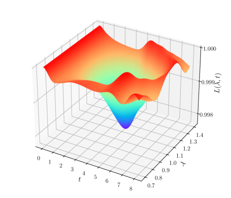
Figure 1: (color online) Time evolution of the biorthogonal LE $L(\lambda,t)$ as the function of $\lambda$ and $t$ for $N=16$ lattice sites with $\gamma=0.5$. It indicates that the decay of biorthogonal LE is enhanced by the quantum criticality and is consistent with the analytical result.

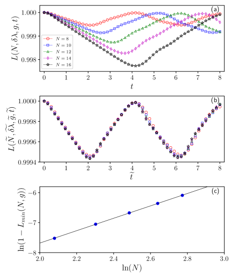
Figure 2: (Color online) Dynamical scaling of the biorthogonal LE at $\gamma=0.5$ in the NHTI chain. (a) The biorthogonal LE $L(N,\delta\lambda,g,t)$ with $\delta\lambda=0.02$ and $g=0.01$ as a function of time for different system sizes, $N=8,10,12,14,16$ (from bottom to top). (b) Scaling invariance of the biorthogonal LE $L(\widetilde{N},\widetilde{\delta\lambda},\widetilde{g},\widetilde{t})$ given in Eq.(9). We take $N=8$, $\delta\lambda=0.02,g=0.01$, $\nu=z=1$ and $b=1$. All other data for $b=4/5,2/3,4/7,1/2$ collapse onto a single curve. (c) Finite-size scaling of the $1-L_{min}$ obtained from (a) as a function of lattice size $N$. The blue circle symbols are the numerical results, and the black solid line is the fitting curve. The critical exponent of the correlation length derived from fitting curve is $\nu=0.968$.

Results.- To compute the ground state and the biorthogonal LE of the NHTI model, we perform the exact diagonalization that can be generated to arbitrary non-integrable models Wang et al. (2020b); Gopalakrishnan and Gullans (2021) with periodic boundary conditions $\sigma_{N+1}^{x}=\sigma_{1}^{x}$. Without loss of generality, we choose $J=1$ and $\gamma=0.5$ for simplicity in our numerical simulations. The ground states are found separately from Eq.(2) and Eq.(3) by the energy minimum as Hermitian models. The time evolution of the right and left ground states are obtained from Eq.(6) and Eq.(7) independently. To see the decay of the biorthogonal LE, we quench the system from an initial $\lambda_{i}$ to a final $\lambda_{f}$ with a small constant step $g=-0.01$ and $\Delta t=0.02$. We note that the $\Delta t$ scales as $\Delta\widetilde{t}=b^{-z}\Delta t$ from the scaling law in Eq.(10) during the simulations. The corresponding biorthogonal LE are calculated from Eq.(8) by varying the initial $\lambda_{i}$. The data of the biorthogonal LE are presented in Fig.1, where a deep valley appears around the critical point $\lambda_{c}=2/\sqrt{3}\approx 1.155$ during the time evolution. This implies that the decay of the biorthogonal LE is highly enhanced by the quantum criticality indicating that the biorthogonal LE can in principle characterize the biorthogonal many-body phase transitions.

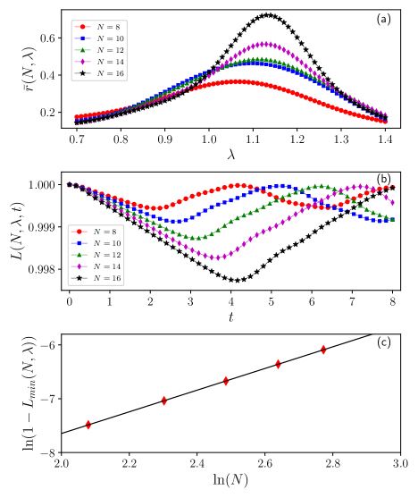
Figure 3: (Color online) Scaling of the rate function and biorthogonal LE in the NHTI model with $\gamma=0.5$. (a) The short-time average rate function $\bar{r}(N,\lambda)$ with respect to $\lambda$ for different lattice sizes, $N=8,10,12,14,16$ (from bottom to top). (b) The biorthogonal LE $L(N,\lambda,t)$ at the peak position of $\bar{r}(N,\lambda)$ in (a) with $g=-0.01$ as a function of time for different lattice sizes, $N=8,10,12,14,16$ (from top to bottom). (c) Finite-size scaling of the $1-L_{min}$ obtained from (b) as a function of lattice size $N$. The red diamond symbols are the numerical values, while the black solid line denotes the fitting curve. The correlation length critical exponent obtained from fitting curve is $\nu=0.993$.

From the renormalization group analysis, the biorthogonal LE is scaling invariance near the critical point under the transformation Eq.(10). To verify the scaling invariance Eq.(9), we first perform numerical calculations at $\lambda=1.15$ (exact $\lambda_{c}\approx 1.155$) by choosing the parameters $\delta\lambda=0.02$, $g=0.01$ and $\gamma=0.5$ for $N=8,10,12,14,16$. The data are represented in Fig.2(a), where the biorthogonal LEs exhibit a decay and revival dynamics separately as Hermitian systems Quan et al. (2006); Hwang et al. (2019). However, if the biorthogonal LEs are derived using the transformation Eq.(10) instead, all LEs collapse onto a single curve using the Ising universal class $\nu=z=1$ as shown in Fig.2(b), confirming the validity of scaling invariance in Eq.(9).

It was shown in Ref.[Hwang et al., 2019], under the conditions $\delta\lambda=0$ and $N^{1/\nu}g\ll 1$, the minimum of the LE scales as,

$$1-L_{min}(N,g)\propto g^{2}N^{2/\nu}$$ (15)

This relation indicates a critically enhanced decay of the LE that can be used to obtain the correlation length critical exponent $\nu$. The values of $1-L_{min}$ are derived from the first minimum of biorthogonal LE from Fig.2(a) and are plotted in Fig.2(c) with respect to the lattice size $N$. By fitting the data, we get the critical exponent $\nu=0.968$ which is consistent with that of the Ising transition in equilibrium. The scaling law in Eq.(15) provides an easy way for studying the quantum criticality. However, it needs to know the critical value $\lambda_{c}$ in advance because of the condition $\delta\lambda=0$, which limits its application to unknown systems.

Motivated by the behavior of critically enhanced decay of LE and the definition of the fidelity susceptibility, we introduce a time-average rate function,

$$\bar{r}(N,\lambda)=-\frac{1}{N}\frac{\ln(\bar{L}(N,\lambda))}{g^{2}},$$ (16)

where, $\bar{L}(N,\lambda)$ is the time average LE that is defined as,

$$\bar{L}(N,\lambda)=\frac{1}{T}\int_{0}^{T}L(N,\lambda,t)dt.$$ (17)

Here, $L(N,\lambda,t)$ is defined in Eq.(8) with $g=\lambda_{i}-\lambda_{f}$. The time average LE that usually demands a very large time $T$ has been used to characterize the phase transition of Ising model in nonzero temperatures recently Zhang and Song (2021). Here, will we show that a short-time average LE can help identifying phase transitions due to the critically enhanced decay behavior.

To achieve it, we first find the pseudo critical point $\lambda_{N}^{\ast}$ for each lattice $N$ using Eq.(16) by varying the control parameter $\lambda$. The pseudo critical value $\lambda_{N}^{\ast}$ is derived from the peak of the time-average rate function as shown in Fig.3(a). We then perform the calculations for a quench by using $\lambda_{i}=\lambda_{N}^{\ast}$ to $\lambda_{f}=\lambda_{N}^{\ast}-g$ with a small $g=-0.01$ to find the minimum $L_{min}(N,\lambda)$ [see Fig.3(b)]. Finally, we extrapolate the critical exponent $\nu$ from the scaling relation Eq.(15) to obtain the correlation length critical exponent [c.f. Fig.3(c)]. We get the critical exponent $\nu=0.993$ from fitting the data which is in agreement with that of Ising transition. Consequently, it offers a more flexible approach to study the quantum criticality. We note that this probe method can apply to both Hermitian and non-Hermitian many-body systems with second-order phase transitions without knowing the critical value in advance. More examples will be given to illustrate this approach in future research.

Conclusion.- In summary, we have studied the finite-size dynamical scaling of the biorthogonal LE in the one-dimensional NHTI model. We have shown that the LE can serve as a probe to detect biorthogonal many-body phase transitions. That is to say, we can probe quantum criticality of non-Hermitian many-body systems from the biorthogonal LE dynamics in experiments without knowing the exact critical values in advance. We note that the concept of the biorthogonal LE of the systems is general for any non-Hermitian many-body Hamiltonian with real eigenvalues. Therefore, it would be possible to apply the biorthogonal LE to understand the critical properties of unknown phase transitions of arbitrary non-Hermitian many-body systems as long as the ground states are well defined. Moreover, it would be more intriguing to know whether the scaling laws of the biorthogonal LE is able to be applicable to non-Hermitian many-body systems with complex eigenvalues in the future.

Acknowledgments.- G.S. would like to thank W.-L. You for useful discussions and comments for the paper. G. S. is appreciative of support from the NSFC under the Grant Nos. 11704186 and 11874220. S. P. K is appreciative of supported by the NSFC under the Grant Nos. 11674026, 11974053. Numerical simulations were performed on the clusters at Nanjing University of Aeronautics and Astronautics.

References

- Sachdev (1999) S. Sachdev, Quantum phase transitions (Cambridge University Press, 1999).
- Levin and Wen (2006) M. Levin and X.-G. Wen, Physical Review Letters 96, 110405 (2006).
- Bergholtz et al. (2021) E. J. Bergholtz, J. C. Budich, and F. K. Kunst, Reviews of Modern Physics 93, 015005 (2021).
- Ashida et al. (2021) Y. Ashida, Z. Gong, and M. Ueda, Advances in Physics 69, 249 (2021).
- Lee (2016) T. E. Lee, Physical Review Letters 116, 133903 (2016).
- Yao and Wang (2018) S. Yao and Z. Wang, Physical Review Letters 121, 086803 (2018).
- Kunst et al. (2018) F. K. Kunst, E. Edvardsson, J. C. Budich, and E. J. Bergholtz, Physical Review Letters 121, 026808 (2018).
- Xiong (2018) Y. Xiong, Journal of Physics Communications 2, 035043 (2018).
- Gong et al. (2018) Z. Gong, Y. Ashida, K. Kawabata, K. Takasan, S. Higashikawa, and M. Ueda, Physical Review X 8, 031079 (2018).
- Martinez Alvarez et al. (2018) V. M. Martinez Alvarez, J. E. Barrios Vargas, and L. E. F. Foa Torres, Physical Review B 97, 121401(R) (2018).
- Yokomizo and Murakami (2019) K. Yokomizo and S. Murakami, Physical Review Letters 123, 066404 (2019).
- Okuma et al. (2020) N. Okuma, K. Kawabata, K. Shiozaki, and M. Sato, Physical Review Letters 124, 086801 (2020).
- Zhang et al. (2020a) K. Zhang, Z. Yang, and C. Fang, Physical Review Letters 125, 126402 (2020a).
- Yang et al. (2020a) Z. Yang, K. Zhang, C. Fang, and J. Hu, Physical Review Letters 125, 226402 (2020a).
- Wang et al. (2020a) X.-R. Wang, C.-X. Guo, and S.-P. Kou, Physical Review B 101, 121116(R) (2020a).
- Jiang et al. (2020) H. Jiang, R. Lü, and S. Chen, The European Physical Journal B 93, 1 (2020).
- Weidemann et al. (2020) S. Weidemann, M. Kremer, T. Helbig, T. Hofmann, A. Stegmaier, M. Greiter, R. Thomale, and A. Szameit, Science 368, 311 (2020).
- Xiao et al. (2020) L. Xiao, T. Deng, K. Wang, G. Zhu, Z. Wang, W. Yi, and P. Xue, Nature Physics 16, 761 (2020).
- Borgnia et al. (2020) D. S. Borgnia, A. J. Kruchkov, and R.-J. Slager, Physical Review Letters 124, 056802 (2020).
- Heiss (2012) W. Heiss, Journal of Physics A: Mathematical and Theoretical 45, 444016 (2012).
- Kozii and Fu (2017) V. Kozii and L. Fu, arXiv preprint arXiv:1708.05841 (2017).
- Hodaei et al. (2017) H. Hodaei, A. U. Hassan, S. Wittek, H. Garcia-Gracia, R. El-Ganainy, D. N. Christodoulides, and M. Khajavikhan, Nature 548, 187 (2017).
- Zhou et al. (2018a) H. Zhou, C. Peng, Y. Yoon, C. W. Hsu, K. A. Nelson, L. Fu, J. D. Joannopoulos, M. Soljačić, and B. Zhen, Science 359, 1009 (2018a).
- Miri and Alu (2019) M.-A. Miri and A. Alu, Science 363, 42 (2019).
- Park et al. (2019) J.-H. Park, A. Ndao, W. Cai, L.-Y. Hsu, A. Kodigala, T. Lepetit, Y.-H. Lo, and B. Kanté, arXiv preprint arXiv:1904.01073 (2019).
- Yang and Hu (2019) Z. Yang and J. Hu, Physical Review B 99, 081102(R) (2019).
- Özdemir et al. (2019) Ş. Özdemir, S. Rotter, F. Nori, and L. Yang, Nature Materials 18, 783 (2019).
- Dóra et al. (2019) B. Dóra, M. Heyl, and R. Moessner, Nature Communications 10, 1 (2019).
- Jin et al. (2020) L. Jin, H. C. Wu, B.-B. Wei, and Z. Song, Physical Review B 101, 045130 (2020).
- Xiao et al. (2021) L. Xiao, T. Deng, K. Wang, Z. Wang, W. Yi, and P. Xue, Physical Review Letters 126, 230402 (2021).
- Matsumoto et al. (2020) N. Matsumoto, K. Kawabata, Y. Ashida, S. Furukawa, and M. Ueda, Physical Review Letters 125, 260601 (2020).
- Yang et al. (2020b) M.-L. Yang, H. Wang, C.-X. Guo, X.-R. Wang, G. Sun, and S.-P. Kou, arXiv e-prints arXiv:2006.10278 , arXiv (2020b).
- Ashida et al. (2017) Y. Ashida, S. Furukawa, and M. Ueda, Nature communications 8, 1 (2017).
- Chang et al. (2020) P.-Y. Chang, J.-S. You, X. Wen, and S. Ryu, Physical Review Research 2, 033069 (2020).
- Lee et al. (2020) E. Lee, H. Lee, and B.-J. Yang, Physical Review B 101, 121109(R) (2020).
- Pan et al. (2020a) L. Pan, X. Chen, Y. Chen, and H. Zhai, Nature Physics 16, 767 (2020a).
- Pan et al. (2020b) L. Pan, X. Wang, X. Cui, and S. Chen, Physical Review A 102, 023306 (2020b).
- Xu and Chen (2020) Z. Xu and S. Chen, Physical Review B 102, 035153 (2020).
- Zhang et al. (2020b) D.-W. Zhang, Y.-L. Chen, G.-Q. Zhang, L.-J. Lang, Z. Li, and S.-L. Zhu, Physical Review B 101, 235150 (2020b).
- Lee (2021) C. H. Lee, Physical Review B 104, 195102 (2021).
- Shackleton and Scheurer (2020) H. Shackleton and M. S. Scheurer, Physical Review Research 2, 033022 (2020).
- Liu et al. (2020) T. Liu, J. J. He, T. Yoshida, Z.-L. Xiang, and F. Nori, Physical Review B 102, 235151 (2020).
- Yang et al. (2021) K. Yang, S. C. Morampudi, and E. J. Bergholtz, Physical Review Letters 126, 077201 (2021).
- Herviou et al. (2019) L. Herviou, N. Regnault, and J. H. Bardarson, SciPost Phys 7, 069 (2019).
- Yoshida et al. (2019) T. Yoshida, K. Kudo, and Y. Hatsugai, Scientific Reports 9, 1 (2019).
- Yoshida et al. (2020) T. Yoshida, K. Kudo, H. Katsura, and Y. Hatsugai, Physical Review Research 2, 033428 (2020).
- Osterloh et al. (2002) A. Osterloh, L. Amico, G. Falci, and R. Fazio, Nature 416, 608 (2002).
- Horodecki et al. (2009) R. Horodecki, P. Horodecki, M. Horodecki, and K. Horodecki, Reviews of Modern Physics 81, 865 (2009).
- Eisert et al. (2010) J. Eisert, M. Cramer, and M. B. Plenio, Reviews of Modern Physics 82, 277 (2010).
- Zanardi and Paunković (2006) P. Zanardi and N. Paunković, Physical Review E 74, 031123 (2006).
- You et al. (2007) W.-L. You, Y.-W. Li, and S.-J. Gu, Physical Review E 76, 022101 (2007).
- Campos Venuti and Zanardi (2007) L. Campos Venuti and P. Zanardi, Physical Review Letters 99, 095701 (2007).
- Gu (2010) S.-J. Gu, International Journal of Modern Physics B 24, 4371 (2010).
- Albuquerque et al. (2010) A. F. Albuquerque, F. Alet, C. Sire, and S. Capponi, Physical Review B 81, 064418 (2010).
- Sun (2017) G. Sun, Physical Review A 96, 043621 (2017).
- Zhu et al. (2018) Z. Zhu, G. Sun, W.-L. You, and D.-N. Shi, Physical Review A 98, 023607 (2018).
- Wei and Lv (2018) B.-B. Wei and X.-C. Lv, Physical Review A 97, 013845 (2018).
- Chen et al. (2008) S. Chen, L. Wang, Y. Hao, and Y. Wang, Physical Review A 77, 032111 (2008).
- Gu et al. (2008) S.-J. Gu, H.-M. Kwok, W.-Q. Ning, and H.-Q. Lin, Physical Review B 77, 245109 (2008).
- Yang et al. (2008) S. Yang, S.-J. Gu, C.-P. Sun, and H.-Q. Lin, Physical Review A 78, 012304 (2008).
- Luo et al. (2018) Q. Luo, J. Zhao, and X. Wang, Physical Review E 98, 022106 (2018).
- Sun et al. (2015) G. Sun, A. K. Kolezhuk, and T. Vekua, Physical Review B 91, 014418 (2015).
- Quan et al. (2006) H. T. Quan, Z. Song, X. F. Liu, P. Zanardi, and C. P. Sun, Physical Review Letters 96, 140604 (2006).
- Hwang et al. (2019) M.-J. Hwang, B.-B. Wei, S. F. Huelga, and M. B. Plenio, eprint arXiv:1904.09937 (2019).
- Mukherjee et al. (2012) V. Mukherjee, S. Sharma, and A. Dutta, Physical Review B 86, 020301(R) (2012).
- Karl et al. (2017) M. Karl, H. Cakir, J. C. Halimeh, M. K. Oberthaler, M. Kastner, and T. Gasenzer, Physical Review E 96, 022110 (2017).
- Pelissetto et al. (2018) A. Pelissetto, D. Rossini, and E. Vicari, Physical Review E 97, 052148 (2018).
- Nigro et al. (2019) D. Nigro, D. Rossini, and E. Vicari, Journal of Statistical Mechanics: Theory and Experiment 2019, 023104 (2019).
- Titum et al. (2019) P. Titum, J. T. Iosue, J. R. Garrison, A. V. Gorshkov, and Z.-X. Gong, Physical review letters 123, 115701 (2019).
- Halimeh et al. (2021) J. C. Halimeh, D. Trapin, M. Van Damme, and M. Heyl, Physical Review B 104, 075130 (2021).
- Dağ and Sun (2021) C. B. Dağ and K. Sun, Physical Review B 103, 214402 (2021).
- Rossini and Vicari (2021) D. Rossini and E. Vicari, Physics Reports 936, 1 (2021).
- Sun et al. (2022) G. Sun, J.-C. Tang, and S.-P. Kou, Frontiers of Physics 17, 1 (2022).
- Tzeng et al. (2021) Y.-C. Tzeng, C.-Y. Ju, G.-Y. Chen, and W.-M. Huang, Physical Review Research 3, 013015 (2021).
- Solnyshkov et al. (2021) D. D. Solnyshkov, C. Leblanc, L. Bessonart, A. Nalitov, J. Ren, Q. Liao, F. Li, and G. Malpuech, Physical Review B 103, 125302 (2021).
- Zhang and Song (2021) K. L. Zhang and Z. Song, Physical Review Letters 126, 116401 (2021).
- Pará et al. (2021) Y. Pará, G. Palumbo, and T. Macrì, Physical Review B 103, 155417 (2021).
- Xu and Chen (2021) Z. Xu and S. Chen, Physical Review A 103, 043325 (2021).
- Zhou et al. (2018b) L. Zhou, Q.-h. Wang, H. Wang, and J. Gong, Physical Review A 98, 022129 (2018b).
- Zhou and Du (2021) L. Zhou and Q. Du, New Journal of Physics 23, 063041 (2021).
- Zhai and Yin (2020) L.-J. Zhai and S. Yin, Physical Review B 102, 054303 (2020).
- Qiu et al. (2019) X. Qiu, T.-S. Deng, Y. Hu, P. Xue, and W. Yi, iScience 20, 392 (2019).
- Wang et al. (2019) K. Wang, X. Qiu, L. Xiao, X. Zhan, Z. Bian, B. C. Sanders, W. Yi, and P. Xue, Nature communications 10, 1 (2019).
- Brody (2013) D. C. Brody, Journal of Physics A: Mathematical and Theoretical 47, 035305 (2013).
- Sternheim and Walker (1972) M. M. Sternheim and J. F. Walker, Physical Review C 6, 114 (1972).
- Zhang and Song (2020) K. L. Zhang and Z. Song, Physical Review B 101, 245152 (2020).
- Lee and Chan (2014) T. E. Lee and C.-K. Chan, Physical Review X 4, 041001 (2014).
- Wang et al. (2020b) C. Wang, M.-L. Yang, C.-X. Guo, X.-M. Zhao, and S.-P. Kou, EPL (Europhysics Letters) 128, 41001 (2020b).
- Gopalakrishnan and Gullans (2021) S. Gopalakrishnan and M. J. Gullans, Physical review letters 126, 170503 (2021).