On the Parabolic Boundary Harnack Principle

Abstract.

We investigate the parabolic Boundary Harnack Principle by the analytical methods developed in [DS1, DS2]. Besides the classical case, we deal with less regular space-time domains, including slit domains.

1. Introduction

1.1. Statement of main results.

In this paper we provide direct analytical proofs of the parabolic Boundary Harnack Inequality for both divergence and non-divergence type operators, in several different settings. Our strategy is based on our earlier works [DS1, DS2] where the elliptic counterparts of these results were obtained. In order to state our theorems precisely, we introduce some notation.

We denote by $\Gamma\subset\mathbb{R}^{n+1}$ the graph of a continuous function $g(x^{\prime},t)$ in the $x_{n}$ direction,

$$\Gamma:=\{x_{n}=g(x^{\prime},t)\},\quad\quad(0,0)\in\Gamma,$$

while $\mathcal{C}_{r}$ denotes the cylinder of size $r$ on top of $\Gamma$ (in the $e_{n}$ direction) i.e.,

$$\mathcal{C}_{r}:=\{(x^{\prime},x_{n},t)|x^{\prime}\in B^{\prime}_{r},\quad t\in(-r^{2},r^{2}),\quad g(x^{\prime},t)<x_{n}<g(x^{\prime},t)+r\}.$$

As usual, $x^{\prime}=(x_{1},\ldots,x_{n-1})$, while $B^{\prime}_{r}\subset\mathbb{R}^{n-1}$ is the ball of radius $r$ centered at the origin.

We consider solutions $u(x,t)$ to the parabolic equation

$$u_{t}=Lu\quad\text{in $\mathcal{C}_{1},$}$$

where $Lu=tr(A(x)D^{2}u)$ or $L(u)=div(A(x)\nabla u)$, with $A$ satisfying,

$$\lambda I\leq A\leq\Lambda I,\quad 0<\lambda\leq\Lambda<+\infty.$$

First, we recall the standard boundary Harnack inequalities for parabolic equations in Lipschitz domains. References to known literature will be provided in the next subsection. Here $g\in C_{x^{\prime},t}^{\alpha,\beta}$ if

$$|g(x^{\prime},t)-g(y^{\prime},s)|\leq C(|x^{\prime}-y^{\prime}|^{\alpha}+|t-s|^{\beta}),$$

and $\overline{E}$, $\underline{E}$ are points interior to $\mathcal{C}_{1}$ at times $t=1/2$ and $t=-1/2$ respectively,

$$\overline{E}=\left(\left(g\left(0,\frac{1}{2}\right)+\frac{1}{2}\right)e_{n},\frac{1}{2}\right),\quad\quad\underline{E}=\left(\left(g\left(0,-\frac{1}{2}\right)+\frac{1}{2}\right)e_{n},-\frac{1}{2}\right).$$

Theorem 1.1 ($C^{1,\frac{1}{2}}$ domains).

Assume that $g\in C_{x^{\prime},t}^{1,\frac{1}{2}}$ and $u,v$ are two positive solutions to

$$u_{t}=Lu,\quad\quad v_{t}=Lv\quad\mbox{in $\mathcal{C}_{1}$,}$$

with $u$ vanishing continuously on $\Gamma$. Then

(1.1) $$\frac{u}{v}\ (x)\leq C\,\,\frac{u(\overline{E})}{v(\underline{E})}\quad\mbox{for all $x\in\mathcal{C}_{1/2}$},$$

with $C$ depending only on $n$, $\|g\|_{C^{1,1/2}},\lambda,$ and $\Lambda$.

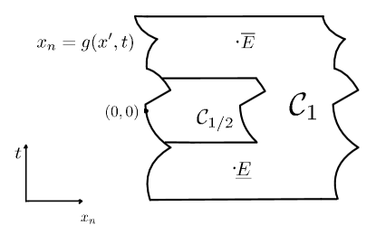
Figure 1. Theorem 1.1.

In this note, we provide new versions of Theorem 1.1 in more general Hölder domains.

Theorem 1.2 ($C^{\frac{1}{2}+,\frac{1}{3}+}$ domains).

Theorem 1.1 holds if $g\in C_{x^{\prime},t}^{\alpha,\beta}$ with $\alpha>1/2$, $\beta>1/3$.

In the case of the heat operator we may lower further the space regularity of $g$ to any exponent $\alpha>0$ provided that we have a $1/2$ Hölder modulus of continuity in time (from one-side).

Theorem 1.3 ($C^{\alpha,\frac{1}{2}}$ domains).

Theorem 1.1 holds for the heat equation if $g\in C_{x^{\prime},t}^{\alpha,\frac{1}{2}}$ with $\alpha>0$.

We remark that the only property of the heat equation needed in the proof of Theorem 1.3 is the translation invariance with respect to the $x_{n},t$ variables. Hence the theorem holds also for operators $L$ with coefficients depending only on the $x^{\prime}$ variable.

Next we state a result in slit-domains, that is the case when the equations are satisfied in the complement of a thin set $S\subset\mathbb{R}^{n+1}$ included in a lower dimensional subspace. This case is relevant for example in the time-dependent Signorini problem.

Precisely we assume that $S$ is a closed set and

$$S\subset\{x_{n}=0\},$$

and in this case

$$\mathcal{C}_{r}=B_{r}\times(-r^{2},r^{2}),\quad\overline{E}=(1/2e_{n},1/2),\,\,\underline{E}=(1/2e_{n},-1/2).$$

With these notation, we state our theorem.

Theorem 1.4 (Thin Parabolic Boundary Harnack).

If $u,v$ are two positive solutions even in the $x_{n}$ variable,

$$u_{t}=Lu\quad\quad v_{t}=Lv,\quad\mbox{in $\mathcal{C}_{1}\setminus S$,}$$

and $u$ vanishes on $S$, then (1.1) holds.

The assumption that $u$, $v$ are even in the $x_{n}$ variable can be removed provided that $\mathcal{C}_{1}\setminus S$ contains a ball of radius $\sigma$ centered on $\{x_{n}=0\}$, and the constant $C$ in estimate (1.1) depends on $\sigma$.

We remark that in Theorems 1.2-1.4 whenever the boundary of the domain contains non-regular points for the Dirichlet problem, the statement that $u$ vanishes on it is interpreted in the sense that $u$ is the limit of a sequence of continuous subsolutions which vanish on it.

1.2. Known literature.

For the last 50 years, the boundary Harnack principle has played an essential role in analysis and PDEs in a variety of contexts. The available literature on this topic is very rich and we collect here only the crucial results, making no attempt to discuss the countless important applications of this fundamental tool.

1.2.1. Elliptic case

In the elliptic context, the classical Boundary Harnack Principle, that is the case when $g$ is Lipschitz continuous, states the following. Here the notation is the same as above, with $u,v,g$ independent on $t$.

Theorem 1.5.

Let $u,v>0$ satisfy $Lu=Lv=0$ in $\mathcal{C}_{1}$ and vanish continuously on $\Gamma$. Assume $u,v$ are normalized so that $u\left(e_{n}/2\right)=v(e_{n}/2)=1,$ then

(1.2) $$C^{-1}\leq\frac{u}{v}\leq C,\quad\text{in $\mathcal{C}_{1/2},$}$$

with $C$ depending on $n,\lambda,\Lambda,$ and the norm of $g$.

The case when $L=\Delta$ first appears in [A, D, K, W]. Operators in divergence form were then considered in [CFMS], while the case of operator in non-divergence form was treated in [FGMS]. The same result for operators in divergence form was extended also to so-called NTA domains in [JK]. The case of Hölder domains and $L$ in divergence form was addressed with probabilistic techniques in [BB1, BBB], and an analytic proof was then provided in [F]. For Hölder domains and operators $L$ in non-divergence form, it is necessary that the domain is $C^{0,\alpha}$ with $\alpha>1/2$ or that it satisfies a uniform density property, and this was first established again using a probabilistic approach [BB2].

In [DS1, DS2] we presented a unified analytic proof the Boundary Harnack Principle that does not make use of the Green’s function and which holds for both operators in non-divergence and in divergence form. The idea is to find an “almost positivity property” of a solution, which can be iterated from scale 1 to all smaller scales (some similar ideas were also used in [KiS, S] to treat non-divergence equations with unbounded drift). This strategy successfully applies to other similar situations like that of Hölder domains, NTA domains, and to the case of slit domains, providing a unified approach to a large class of results.

1.2.2. Parabolic case.

For parabolic equations the situation is more complicated, essentially due to the evolution nature of the latter which is reflected in a time-lag in the Harnack Principle. For operators in divergence form, the parabolic boundary Harnack principle in Theorem 1.1 is due to [K2, FGS, Sal]. In the case of operators in non-divergence form in cylinders with $C^{2}$ cross sections, Theorem 1.1 was settled in [G], where the author also derived a Carleson estimate (see Lemma 2.6) in Lipschitz domains. The statement of Theorem 1.1 in Lipschitz domain was later obtained in [FSY], which is (to the authors knowledge) the first instance in which a boundary Harnack type result in Lipschitz domains is obtained without the aid of Green’s functions (and it is probably the inspiration for the later works in the elliptic context [KiS, S]). In [HLN], Theorem 1.1 was also shown to hold for unbounded parabolically Reifenberg flat domains. In the context of time independent Hölder domains, a result in the spirit of Theorem 1.2 was obtained via probabilistic techniques in [BB]. The result in Theorem 1.3 is completely novel. Concerning slit domains, in the case when $S$ is the subgraph of a parabolic Lipschitz graph, the thin-version Theorem 1.4 was established by [PS]. Again, our strategy provides a unified approach for a variety of contexts.

1.3. Organization of the paper.

The paper is organized as follows. In Section 2, after recalling some standard results, we provide the proof of Theorems 1.1 and 1.4. The key “almost positivity” property to be iterated from scale 1 to all smaller scales, is obtained in Lemma 2.5. The following section deals with Hölder domains and the proof of Theorem 1.2, which relies on the same strategy as Theorem 1.1, though the proof of the Carleson estimate in the Hölder setting requires a more involved argument similar to the one in the proof of Lemma 2.5. Section 4 contains the proof of Theorem 1.3, which is based on refined versions of the weak Harnack inequality (see Lemmas 4.2-4.4).

2. Proof of Theorem 1.1 and 1.4

In this section, we provide the proof of the classical result Theorem 1.1 and the novel result Theorem 1.4. We start by collecting standard known Harnack type inequalities. In the divergence setting these results are due to [M], while in the non-divergence setting they follow from [Wa].

2.1. Weak Harnack inequality

Denote by

$$Q_{r}:=(-r,r)^{n}\times(-r^{2},0],\quad\quad Q_{r}(x_{0},t_{0}):=(x_{0},t_{0})+Q_{r},$$

the parabolic cubes of size $r$. The parabolic boundary of $Q_{r}$ is denoted by $\partial_{p}Q_{r}$ and is given by:

$$\partial_{p}Q_{r}:=(\partial(-r,r)^{n}\times(-r^{2},0))\cup((-r,r)^{n}\times\{-r^{2}\}).$$

Similarly,

$$Q^{\prime}_{r}:=(-r,r)^{n-1}\times(-r^{2},0],\quad\quad Q^{\prime}_{r}(x^{\prime}_{0},t_{0}):=(x^{\prime}_{0},t_{0})+Q^{\prime}_{r}.$$

Our main tools in establishing the boundary Harnack inequalities are the standard weak Harnack estimates. We recall the parabolic versions which as mentioned in the introduction differ from the elliptic counterparts due to the time-lag.

Theorem 2.1 (Supersolution).

If

$$u_{t}\geq Lu\quad\mbox{and}\quad u\geq 0\quad\quad\mbox{in $Q_{1}$},\quad u(0,0)=1,$$

then

$$\int_{Q_{\frac{1}{2}}(0,-\frac{1}{2})}u^{p}\,dxdt\leq C,$$

for some $p>0$ small, $C$ large universal (i.e. dependent on $n,\lambda,\Lambda$).

Theorem 2.2 (Subsolution).

If

$$u_{t}\leq Lu\quad\mbox{and}\quad u\geq 0\quad\quad\mbox{in $Q_{1}$},$$

then

$$u(0,0)\leq C(p)\|u\|_{L^{p}(Q_{1})},$$

for any $p>0$.

The classical (backward) Harnack inequality then reads as follows.

Theorem 2.3 (Harnack inequality).

If

$$u_{t}=Lu\quad\mbox{and}\quad u\geq 0\quad\quad\mbox{in $Q_{1}$},$$

then for $c$ small universal (dependent on $n,\lambda,\Lambda$),

$$\min_{Q_{1/2}}u\geq c\,\,\max_{Q_{1/2}(0,-\frac{1}{2})}u.$$

Another useful version for the subsolution property is the following measure to pointwise estimate.

Theorem 2.4 (Subsolution).

If

$$u_{t}\leq Lu\quad\mbox{and}\quad 1\geq u\geq 0\quad\quad\mbox{in $Q_{2}$},$$

and for some $\delta>0,$

$$|\{u=0\}\cap Q_{1}(0,-1)|\geq\delta.$$

Then

$$u\leq 1-c(\delta)\quad\mbox{in}\quad Q_{1}.$$

With these tools at hand, we are ready to provide in the following subsection our proof of the classical result in Theorem 1.1.

2.2. Proof of Theorem 1.1

In what follows, constants depending on $n,\lambda,\Lambda$, and the norm of $g$, are called universal.

We denote by

$$\mathcal{C}_{r}^{-}:=\{(x^{\prime},x_{n},t)|\,\,x^{\prime}\in(-r,r)^{n-1},\quad t\in(-r^{2},0],\quad g(x^{\prime},t)<x_{n}<g(x^{\prime},t)+r\},$$

the backward in time cylinder of size $r$ on top (in the $e_{n}$ direction) of the graph $\Gamma$ of $g$. Also we set,

$$\mathcal{A}_{r}:=\left\{(x,t)\in\mathcal{C}_{r}^{-}|\quad g(x^{\prime},t)+\delta r\leq x_{n}<g(x^{\prime},t)+r\right\},$$

that is the collection of points in the cylinder $\mathcal{C}^{-}_{r}$ at height greater or equal than $\delta r$ on top of $\Gamma$, for some $\delta>0$ small, to be made precise later.

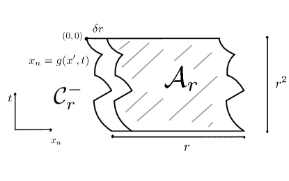
Figure 2. The sets $\mathcal{C}_{r}^{-}$ and $\mathcal{A}_{r}$.

The key tool for establishing the boundary Harnack estimates is the following iterative lemma. Later we will apply this lemma for the difference $w=v-cu$ for some sufficiently small constant $c$, in order to obtain the desired claim in Theorem 1.1.

Lemma 2.5.

There exist universal constants $M$, $\delta>0$, such that if $w$ is a solution to

$$w_{t}=Lw\quad\mbox{ in}\quad\mathcal{C}^{-}_{r},$$

(possibly changing sign) with $w^{-}$ vanishing continuously on $\Gamma$,

(2.1) $$w\geq M\quad\quad\text{in}\quad\mathcal{A}_{r},$$

and

$$w\geq-1\quad\text{in $\mathcal{C}^{-}_{r}$},$$

then,

(2.2) $$w\geq M\,a\quad\text{in $\mathcal{A}_{\frac{r}{2}}$},$$

and

(2.3) $$w\geq-a\quad\text{in $\mathcal{C}^{-}_{\frac{r}{2}}$},$$

for some small $a>0$.

The conclusion can be iterated indefinitely and we obtain that if the hypotheses are satisfied in $\mathcal{C}^{-}_{r}$ then

(2.4) $$w>0\quad\text{on the line segment $\{(se_{n},0),\quad 0<s<r\}.$}$$

Proof.

We start by observing that any point $(x_{0},t_{0})\in\mathcal{A}_{r/2}$ can be connected through a chain of backwards-in-time adjacent parabolic cubes of size $\bar{r}:=c_{1}\delta r$ centered at

$$(x_{j},t_{j}):=(x_{0}+j\bar{r}e_{n},t_{0}-j\bar{r}^{2}),$$

to a last cube $Q_{\bar{r}}(x_{m},t_{m})\subset\mathcal{A}_{r}$ (see Figure 2). Here $c_{1}$ is small depending on the $C_{x^{\prime},t}^{1,1/2}$ norm of $g$ so that

$$Q_{2\bar{r}}(x_{j},t_{j})\subset\mathcal{C}_{r}^{-},$$

and the number $m$ of cubes depends only on $c_{1}$. By Harnack inequality (Theorem 2.3) applied to $w+1\geq 0$, using assumption (2.1), we get

$$(w+1)(x_{0},t_{0})\geq c^{m}(M+1)\quad\Longrightarrow\quad w\geq 1\quad\mbox{in}\quad\mathcal{A}_{r/2},$$

provided that we choose $M$ large depending on $c_{1}$ (and independent of $\delta$). Hence (2.2) holds with $a=1/M$.

To establish (2.3) with this choice of $M,a$, we first extend $w^{-}=0$ in

$$Q^{\prime}_{r}\times(\{x_{n}<g(x^{\prime},t)\}\cup\{x_{n}>g(x^{\prime},t)+\delta r\}),$$

so that $w^{-}$ is a global subsolution in $Q^{\prime}_{r}\times\mathbb{R}$ thanks to assumption (2.1).Then, for each cube $Q_{2\delta r}(x,t)$ satisfying $Q^{\prime}_{2\delta r}(x^{\prime},t)\subset Q^{\prime}_{r},$ we have

$$|\{w^{-}=0\}\cap Q_{2\delta r}(x,t)|\geq\frac{1}{2}|Q_{2\delta r}(x,t)|.$$

This is a consequence of the graph property of $\Gamma$. Indeed, for each fixed $(x^{\prime},t)$, we consider the 1D line in the $e_{n}$ direction. Any segment of length $2\delta r$ on this line has at least half of its length either in $\mathcal{A}_{r}$ or in the complement of $\mathcal{C}_{r}^{-}$.

By weak Harnack inequality, Theorem 2.4, as we remove the collection of cubes $Q_{2\delta r}(x,t)$ which are tangent to the parabolic boundary of $Q^{\prime}_{r}\times\mathbb{R}$, the norm $\|w^{-}\|_{L^{\infty}}$ decays by a factor $1-c$, $c>0$ universal. Iterating this for $\sim 1/\delta$ times we find that

$$w^{-}\leq(1-c)^{1/\delta}\quad\mbox{in $\mathcal{C}^{-}_{r/2}\subset Q^{\prime}_{r/2}\times\mathbb{R}$.}$$

We choose $\delta$ small, so that $w^{-}\leq a=M^{-1}$ and (2.3) holds.

∎

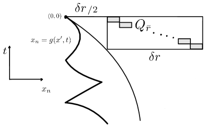
Figure 3. Proof of Lemma 2.5.

A second ingredient in the proof of Theorem 1.1 is the following Carleson estimate which provides a bound for $u$ in the cylinder $\mathcal{C}_{2/3}$.

Lemma 2.6 (Carleson estimate).

Let $u,\bar{E}$ be as in Theorem 1.1, then

$$\|u\|_{L^{\infty}(\mathcal{C}_{2/3})}\leq C\,u(\overline{E}),$$

with $C>0$ universal.

Proof.

The Carleson estimate can be established by similar arguments as in the Lemma 2.5 above. We will use this approach in the case of Hölder domains in the next section. However, for $C_{x^{\prime},t}^{1,\frac{1}{2}}$ domains, the Carleson estimate is a direct consequence of the weak Harnack inequality.

Indeed, assume that $u(\overline{E})=1$. Any point $(x_{0},t_{0})\in\mathcal{C}_{12/17}$ can be connected to $\overline{E}$ by a chain of forward-in-time adjacent cubes $Q_{r_{j}}(x_{j},t_{j})$ included in $\mathcal{C}_{1}$, with $r_{j}$ proportional to the parabolic distance $d_{j}$ from $(x_{j},t_{j})$ to $\Gamma$. The number of cubes in this chain is proportional to $|\log d_{0}|$. By Harnack inequality,

$$u(x_{0},t_{0})\leq\,e^{C|\log d_{0}|}u(\overline{E})\,\leq d_{0}^{-C^{\prime}}.$$

This means that $\|u\|_{L^{p}}\leq C$ in $\mathcal{C}_{12/17}$ for some small $p>0$ universal. The extension of $u$ by $0$ in $\Omega_{r}:=((-r,r)^{n-1}\times(-r^{2},r^{2}))\times\{x_{n}\leq g(x^{\prime},t)\}$ is a subsolution, and now we can apply weak Harnack inequality Theorem 2.2 in cubes $Q_{c_{0}}(x,t)\subset\mathcal{C}_{12/17}\cup\Omega_{r}$ for $(x,t)\in\mathcal{C}_{2/3}$ and $c_{0}$ small universal, to obtain the desired conclusion.

∎

We are now ready to combine the previous two lemmas and obtain the desired Theorem 1.1.

Proof of Theorem 1.1.

We assume that $u(\bar{E})=v(\underline{E})=1$ and define $w=C_{1}v-c_{1}u$. By Harnack inequality applied to $v$ and the Carleson estimate for $u$, we can choose the constants $C_{1}$ large, $c_{1}$ small (depending on $\delta$, $M$) such that $w$ satisfies

$$w\geq-1\quad\text{in $\mathcal{C}_{2/3},$}\quad\mbox{and}\quad w(x,t)\geq M\quad\mbox{if}\quad x_{n}\geq g(x^{\prime},t)+\delta/4.$$

Then we can apply Lemma 2.5 in cylinders $\mathcal{C}^{-}_{1/6}$ around any point on $\Gamma\cap\mathcal{C}_{1/2}$, and conclude from (2.4) that $w>0$ in $\mathcal{C}_{1/2}$. ∎

2.3. Proof of Theorem 1.4

The proof is identical to the one of Theorem 1.1 after the appropriate modifications in the definitions of $\mathcal{C}_{r}^{-}$ and $\mathcal{A}_{r}$. Precisely,

$$\mathcal{C}_{r}^{-}:=Q_{r}\setminus S,\quad\quad\mathcal{A}_{r}:=Q_{r}\cap\{|x_{n}|\geq\delta r\}.$$

Lemma 2.5 applies for the difference $w=v-cu$. The hypotheses that $u$ and $w^{-}=(cu-v)^{+}$ vanish on $S$ are understood in the sense that each of them is obtained in $\mathcal{C}_{1}^{-}$ as a pointwise limit of an increasing sequence of continuos subsolutions in $Q_{1}$ which vanish on $S$. Notice that if $u_{n}$ is such a sequence for $u$, then $(c\,u_{n}-v)^{+}$ is a corresponding sequence for $w^{-}$, (since $v\geq 0$ in $\mathcal{C}_{1}^{-}$). Thus, the extensions of $u$ and $w^{-}$ by $0$ on $S$ are subsolutions in $Q_{1}$, and Lemmas 2.5 and 2.6 hold as above.

∎

3. Hölder domains and the proof of Theorem 1.2

In this section we prove Theorem 1.2 by extending the arguments of the previous section to Hölder domains. We assume that for some $\alpha>\frac{1}{2}$,

(3.1) $$[g]_{C_{x^{\prime},t}^{\alpha,\frac{\alpha}{1+\alpha}}}\leq K,$$

for some constant $K$. Below, constants depending possibly on $n,\lambda,\Lambda,\alpha$ and $K$ are called universal.

We define

$$\mathcal{C}_{r}^{-}:=\{(x^{\prime},x_{n},t)|\,\,x\in(-r,r)^{n},\quad t\in(-r,0],\quad g(x^{\prime},t)<x_{n}<g(x^{\prime},t)+r\},$$

and notice that here we took the time interval of $\mathcal{C}_{r}^{-}$ of size $r$ instead of the natural parabolic scaling $r^{2}$ that we used in the previous section. This change is due to the fact that the norm of $g$ is no longer left invariant by the parabolic scaling. We also define

$$\mathcal{A}_{r}:=\left\{x\in\mathcal{C}_{r}^{-}|\quad g(x^{\prime},t)+r^{\beta}\leq x_{n}<g(x^{\prime},t)+r\right\},$$

the points in the cylinder $\mathcal{C}^{-}_{r}$ at height greater or equal than $r^{\beta}$ on top of $\Gamma$, for some $\beta>1$ to be made precise later.

Lemma 3.1.

Suppose (4.3) holds for $\mathcal{C}_{r}^{-}$ and let $w$ be a solution to

$$w_{t}=Lw\quad\mbox{ in}\quad\mathcal{C}^{-}_{r},$$

for which $w^{-}$ vanishes on $\Gamma$. There exist universal constants $C_{0},\beta>0$ such that if

$$w\geq f(r)\quad\quad\text{on}\quad\mathcal{A}_{r},$$

and

$$w\geq-1\quad\text{on $\mathcal{C}^{-}_{r}$},$$

where

$$f(r):=e^{C_{0}r^{\gamma}},\quad\gamma:=\beta(1-\frac{1}{\alpha})<0,$$

then,

(3.2) $$w\geq f(\frac{r}{2})\,\,a\quad\text{on $\mathcal{A}_{\frac{r}{2}}$},$$

and

(3.3) $$w\geq-a\quad\text{on $\mathcal{C}^{-}_{\frac{r}{2}}$},$$

for some small $a=a(r)>0$, as long as $r\leq r_{0}$ universal.

Proof.

We adapt the argument of Lemma 2.5 in this case and sketch the details.

We connect a point $(x_{0},t_{0})\in\mathcal{A}_{r/2}$ (which is not in $\mathcal{A}_{r}$) to a point $(x_{m},t_{m})$ with $x_{m}=x_{0}+r^{\beta}e_{n}\in\mathcal{A}_{r}$ by a chain of adjacent backward-in-time cubes of size $\bar{r}:=c_{0}\,r^{\beta/\alpha}$. The number $m$ of cubes depends on $r$, i.e.

$$m\sim r^{\beta}/\bar{r}=c_{0}^{-1}r^{\beta(1-\frac{1}{\alpha})}=c_{0}^{-1}r^{\gamma}.$$

All the cubes are included in the domain ($t_{m}:=t_{0}-m\bar{r}^{2}$)

$$\left\{(x-x_{0})\cdot e_{n}\geq 0,\quad t\in[t_{m},t_{0}],\quad(x-x_{0})^{\prime}\in[-\bar{r},\bar{r}]^{n-1}\right\},$$

which by (4.3) is included in $\mathcal{C}_{r}^{-}$ since $m\bar{r}^{2}\sim r^{\beta}\bar{r}=c_{0}r^{\beta\frac{\alpha+1}{\alpha}}$, and $c_{0}$ is chosen small. Moreover, $Q_{\bar{r}}(x_{m},t_{m})\subset\mathcal{A}_{r}$, and Harnack inequality for $w+1$ implies that

(3.4) $$w+1\geq f(r)e^{-Cm}\geq 2\quad\quad\mbox{in $\mathcal{A}_{r/2}$,}$$

where the last inequality is guaranteed if we choose $C_{0}$ sufficiently large.

For the second step which bounds $w^{-}$ we use cylinders of size $2r^{\beta}$ (instead of $2\delta r$ as before) and get by the same argument as in the Lipschitz case

(3.5) $$w^{-}\leq e^{-cr^{1-\beta}}=:a.$$

The conclusion follows since in $\mathcal{A}_{r/2}$, $w\geq 1\geq f(r/2)a$, and in the last inequality we used $1-\beta<\gamma$, provided that $\beta$ is chosen sufficiently large.

∎

Lemma 3.2 (Carleson estimate).

Let $u,\bar{E}$ be as in Theorem 1.2. Then,

$$\|u\|_{L^{\infty}(\mathcal{C}_{1/2})}\leq C\,u(\overline{E}),$$

with $C$ universal.

Proof.

We apply an iterative argument similar to the one of Lemma 3.1 above.

Assume $u(\overline{E})=1$, and denote by $h_{\Gamma}$ the distance in the $e_{n}$ direction between a point $(x,t)\in\mathcal{C}_{1}$ and $\Gamma$

$$h_{\Gamma}(x,t):=x_{n}-g(x^{\prime},t).$$

Any point $(x,t)\in\mathcal{C}_{2/3}$ can be connected to $\overline{E}$ by a chain of adjacent forward-in-time cubes included in $\mathcal{C}_{r}$, so that the size of each cube is proportional to the distance from its center to $\Gamma$ raised to the power $1/\alpha$. The Hölder continuity of $g$ implies that the number of cubes in this chain is proportional to $(h_{\Gamma}(x,t))^{1-1/\alpha}$, and by Harnack inequality we find

(3.6) $$u\leq e^{\,C_{1}h_{\Gamma}^{1-1/\alpha}}\quad\quad\text{in $\mathcal{C}_{2/3}$},$$

with $C_{1}$ universal.

With the same notation as in Lemma 3.1, we wish to prove that if $r\leq r_{0}$ and

$$u(y,t_{y})\geq f(r),$$

for some $(y,t_{y})\in\mathcal{C}_{1/2}$, then we can find $(z,t_{z})\in\mathcal{S}$,

$$\mathcal{S}:=\left\{(x,t)|\quad x^{\prime}-y^{\prime}\in(-r,r)^{n-1},\quad t\in(t_{y}-r,t_{y}],\quad 0<h_{\Gamma}(x,t)<r^{\beta}\right\},$$

such that

$$u(z,t_{z})\geq f\left(\frac{r}{2}\right).$$

Since $|(z,t_{z})-(y,t_{y})|\leq Cr^{\alpha}$, we see that for $r$ small enough, we can build a convergent sequence of points $(y_{k},t_{k})\in\mathcal{C}_{2/3}$ with $u(y_{k},t_{k})\geq f(2^{-k}r)\to\infty$. This is a contradiction if we assume that $u$ vanishes continuously on $\Gamma$, and is therefore bounded. If $u=0$ on $\Gamma$ is understood in the sense that $u$ is the limit of an increasing sequence of continuous subsolutions which vanish on $\Gamma$, then we may apply the argument below to one such subsolution and reach again a contradiction.

To show the existence of the point $z$, assume for simplicity $y^{\prime}=0$, $t_{y}=0$ and then $\mathcal{S}=\mathcal{C}^{-}_{r}\setminus\mathcal{A}_{r}$. Let

$$w:=\left(u-\frac{1}{2}e^{C_{0}r^{\gamma}}\right)^{+},\quad\quad\mbox{with}\quad C_{0}\gg C_{1}.$$

By (3.6) we know that

$$w=0\quad\mbox{ in $\mathcal{A}_{r}$}.$$

If our claim is not satisfied then we apply Weak Harnack inequality for $w$ in cubes of size $2r^{\beta}$ repeatedly as in Lemma 3.1. As we move a distance $r$ inside the domain we obtain

(3.7) $$w\leq f\left(\frac{r}{2}\right)\,\,e^{-c_{0}r^{1-\beta}}\quad\text{in $\mathcal{C}^{-}_{r/2}$}.$$

In particular

$$\frac{1}{2}f(r)\leq w(y,t)\leq f\left(\frac{r}{2}\right)e^{-c_{0}r^{1-\beta}},$$

and we reach a contradiction if $r_{0}$ is sufficiently small as long as $1-\beta<\gamma$ (which is possible because $\alpha>1/2$).

∎

4. Proof of Theorem 1.3

In this section we assume that (4.3) holds for some $\alpha>0$ possibly small, and in addition $g$ satisfies a one-sided $C^{1/2}$ bound in the $t$ variable, i.e.

(4.1) $$g(x^{\prime},t+s)-g^{\prime}(x^{\prime},t)\geq-Ks^{1/2},\quad\quad\mbox{if $s\geq 0$}.$$

We will improve the estimates (3.5), (3.7) of the previous section by applying weak Harnack inequality in parabolic cubes of smaller size $\bar{r}\sim r^{\beta/\alpha}$ (which is the size chosen in the first step to obtain (3.4)) instead of $r^{\beta}$. Then the oscillation of $w^{-}$ (or $w$) will decay by a factor $e^{-cr^{1-\beta/\alpha}}$ as we go from $\mathcal{C}_{r}^{-}$ to $\mathcal{C}_{r/2}^{-}$. However, in cubes of size $\bar{r}$ we can no longer guarantee the uniform measure estimate of the set where $w^{-}=0$. To deal with this, we introduce a notion of parabolic capacity for the heat equation. This allows us to diminish the oscillation of $w^{-}$ more precisely than in the measure estimate of Theorem 2.4.

Definition 4.1.

Let $E$ be a closed set. Set,

$$cap_{Q_{1}}(E):=\varphi(0,1)$$

where $\varphi$ is the solution to the heat equation in $Q_{2}(0,1)\setminus(E\cap\overline{Q}_{1})$ which equals 0 on the parabolic boundary of $Q_{2}(0,1)$ and it is equal to 1 in $E\cap\overline{Q}_{1}$.

The function $\varphi$ is well-defined by the Perron-Wiener-Brelot-Bauer theory (see for example [Fr]). Similarly, we can define $cap_{Q_{r}(x,t)}(E)$ by translating the cube at the origin, and then performing a parabolic rescaling

$$cap_{Q_{r}(x,t)}(E):=cap_{Q_{1}}(\tilde{E}),\quad\quad\tilde{E}:=\{(y,s)|(x+r^{2}y,t+rs)\in E\}.$$

We prove here two lemmas about weak Harnack inequality depending on the size of the capacity of $E$ in $Q_{1}$. The first lemma states that a solution to the heat equation in $Q_{1}\setminus E$ satisfies the Harnack inequality in measure if $E$ has small capacity.

Lemma 4.2.

Assume $v\geq 0$ is defined in $Q_{1}\setminus E$ and satisfies

$$v_{t}=\triangle v.$$

Let

$$Q^{i}:=Q_{1/4}(x_{i},t_{i})\subset Q_{1},\quad i=1,2$$

be two cubes of size $1/4$ included in $Q_{1}$, with $t_{2}-t_{1}\geq 1/4$. Assume that

$$cap_{Q_{1}}(E)\leq\delta\quad\mbox{and}\quad\frac{|\{v\geq 1\}\cap Q^{1}|}{|Q^{1}|}\geq 1/2,$$

for some $\delta$ small universal. Then

$$\frac{|\{v\geq c_{0}\}\cap Q^{2}|}{|Q^{2}|}\geq 1/2$$

for some $c_{0}$ small universal.

Proof.

Let $h$ be the solution to the heat equation in $Q_{1}\setminus K$ with $h=0$ on the parabolic boundary of $Q_{1}$, and $h=1$ on $K:=\{v\geq 1\}\cap Q^{1}$. We claim that

$$v\geq h-\varphi\quad\mbox{in $Q_{1}\setminus E$,}$$

where $\varphi$ is the function from Definition 4.1. Since both $v$ with $h-\varphi$ solve the heat equation in $Q_{1}\setminus(K\cup E)$, it suffices to check the claim on the parabolic boundary of $Q_{1}\setminus E$ and on $K$.

Indeed, $v\geq 0\geq h-\varphi$ on $\partial_{p}Q_{1}$, and $v\geq 1\geq h-\varphi$ on $K$. Moreover, $h\leq 1\leq\varphi$ on $E$ gives $h-\varphi\leq 0$ on $E$, and since $v\geq 0$ the claim is proved.

The conclusion follows from the inequality above, since by the Weak Harnack inequality, there exists $c_{0}$ small universal such that $h\geq 2c_{0}$ in $Q^{2}$. On the other hand, $\varphi(0,1)=cap_{Q_{1}}E\leq\delta$ implies that $\varphi\leq c_{0}$ in half the measure of $Q^{2}$ provided that $\delta$ is chosen sufficiently small.

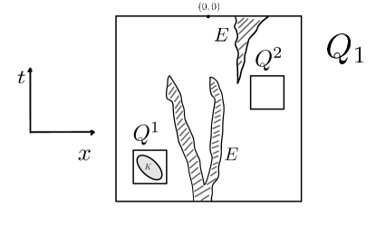
Figure 4. Lemma 4.2.

∎

Remark 4.3.

We may use cubes $Q^{i}$ of size $\sigma$ and with $t_{2}-t_{1}\geq\sigma^{2}$, as long as $\delta$ and $c_{0}$ are allowed to depend on $\sigma$ as well.

The second lemma states that the weak Harnack inequality holds for a subsolution $v\geq 0$ which vanishes on a set $E$ of positive capacity. It follows directly from the definition of $cap_{Q_{1}}(E)$.

Lemma 4.4.

Assume that $v\geq 0$ in $Q_{2}(0,1)$, and

$$\triangle v\geq v_{t} Q_{2}(0,1) v=0 E\cap\overline{Q}_{1}$$ in , and in .

If for some $\delta>0$

$$cap_{Q_{1}}(E)\geq\delta,$$

then

$$v(x,t)\leq(1-c(\delta))\|v\|_{L^{\infty}},\quad(x,t)\in Q_{1/2}(0,1).$$

Proof.

Assume $\|v\|_{L^{\infty}}=1$. We compare $1-v$ with $\varphi$ in $Q_{2}(0,1)\setminus(E\cap\overline{Q}_{1})$ and find $1-v\geq\varphi$. On the other hand since $\varphi(0,1)\geq\delta$ and $\varphi=0$ on the lateral boundary of $Q_{2}(1,0)\times[0,1]$ it follows that $\varphi$ satisfies the forward Harnack inequality, and $\varphi\geq c\delta$ in $Q_{1/2}(0,1)$. The same inequality holds for $1-v$ which gives the desired estimate.

∎

Remark 4.5.

We may write the conclusion in $[-1/2,1/2]^{n}\times[\sigma,1]$ for any $\sigma>0$ provided that the constant $c=c(\delta,\sigma)$ depends on $\sigma$ as well.

We are now ready to provide the proof of Theorem 1.3.

Proof of Theorem 1.3. We only show that the exponent in the estimate (3.5) from the previous section can be improved to

(4.2) $$w^{-}\leq e^{-cr^{1-\frac{\beta}{\alpha}}},$$

by the use of the two lemmas above. The rest of the proof remains the same as before. Notice that now $1-\frac{\beta}{\alpha}<\gamma$ holds simply by choosing $\beta>1$ and no restriction on range of the Hölder exponent $\alpha>0$ is needed.

The same argument improves the exponent in (3.7) from $1-\beta$ to $1-\beta/\alpha$ in the proof of the Carleson estimate.

We proceed with the proof of (4.2). We set $\bar{r}:=r^{\beta/\alpha}$, and by hypothesis, the translation by the vector

$$T:=(-\bar{r}e_{n},\kappa\,\bar{r}^{2})\,\,\in\mathbb{R}^{n+1}$$

maps the complement of $\mathcal{C}_{1}$ into itself, provided that $\kappa\leq 1/2$ is small depending on the constant $K$ in (4.1). Thus if we take a cube and then translate it by $T$, the complement of $\mathcal{C}_{1}$ (where $w^{-}=0$) “increased” in the translating cube because of (4.1) (see Figure 5).

Decompose the space $\mathbb{R}^{n+1}$ into cubes of size $Q_{\bar{r}}$ in the following way. Take $Q_{\bar{r}}$ centered at the origin and then translate it by a linear combination of the vectors $\bar{r}e_{i}$, $i<n$, $T$ and $\bar{r}^{2}e_{n+1}$ using integer coefficients. We look at the behavior of $w$ on arrays of cubes translated by multiples of $T$. Starting with $Q_{\bar{r}}(0)$, we consider $Q_{\bar{r}}(mT)$, with $m\in\mathbb{Z}$. When $m\geq C\bar{r}^{\alpha-1}$, $Q_{3\bar{r}}(mT)\subset\mathcal{A}_{r}$, and when $m\leq-C\bar{r}^{\alpha-1}$, $Q_{\bar{r}}(mT)\subset E$, where $E$ denotes the complement of $\mathcal{C}_{1}$. Thus, there is an intermediate $m_{0}$ where

$$cap_{Q_{3\bar{r}}(mT)}(E)<\delta\quad\mbox{ if and only if $m\geq m_{0}$.}$$

When we decrease $m$ from $C\bar{r}^{\alpha-1}$ to $m_{0}$ we may apply Lemma 4.2 in each such $Q_{3\bar{r}}(mT)$. The weak Harnack inequality holds in measure in these cubes (see Remark 4.3, with $\sigma^{2}=\kappa/20$), and as in (3.4), (as there are at most $C\bar{r}^{\alpha-1}$ such cubes) we find that

$$\{w+1\geq f(r)e^{-C\bar{r}^{\alpha-1}}\geq 2\}$$

in a fixed proportion of each such $Q_{3\bar{r}}(mT)$ with $m\geq m_{0}$. Thus $w^{-}=0$ in a fixed proportion of $Q_{3\bar{r}}(mT)$, and by the weak Harnack inequality

(4.3) $$\|w^{-}\|_{L^{\infty}(Q_{\bar{r}}(x,t))}\leq(1-c)\|w^{-}\|_{L^{\infty}(Q_{6\bar{r}}(x,t))}\quad\quad(x,t)=mT+2\bar{r}^{2}e_{n+1},$$

if $m\geq m_{0}$.

If $m<m_{0}$ then the capacity of $E$ in $Q_{3\bar{r}}(mT)$ is more than $\delta$. By Lemma 4.4, the inequality above remains valid after possibly relabeling $c$. We conclude that (4.3) is valid for all cubes centered at $mT+2\bar{r}^{2}e_{n+1}$, and in particular for $Q_{\bar{r}}(2\bar{r}^{2}e_{n+1})$.

This argument shows that (4.3) holds in fact at all points $(x,t)\in\mathcal{C}^{-}_{3r/4}$. Indeed,

if $$|x_{n}-g(x^{\prime},t)|>Cr^{\beta} Q_{\bar{r}}(x,t)\subset\mathcal{A}_{r} Q_{\bar{r}}(x,t)\subset E$$ then either or

and $\eqref{4000}$ is satisfied trivially as $w^{-}=0$ in $Q_{\bar{r}}(x,t)$. Otherwise, we argue as above by decomposing the space starting with the cube centered at $(x,t)-2\bar{r}^{2}e_{n+1}$ instead of the origin. Notice that $(x,t)\in\mathcal{C}^{-}_{3r/4}$ and $|x_{n}-g(x^{\prime},t)|\leq Cr^{\beta}$ imply that

$$Q_{3\bar{r}}((x,t)-mT)\subset\mathcal{A}_{r} Q_{3\bar{r}}((x,t)+mT)\subset E m\sim C\bar{r}^{\alpha-1}$$ and when

and the argument applies as before.

In conclusion, the maximum of $w^{-}$ is decaying a fixed proportion each time we remove the cubes $Q_{6\bar{r}}$ which are tangent to the parabolic boundary of the infinite cylinder in the $(x^{\prime},t)$ variables

$$\{|x_{i}|\leq 3/4r,\quad i<n\}\cap\{t\in[-3/4\,r,0]\}.$$

Thus

$$w^{-}\leq e^{-cr\bar{r}^{-1}}\quad\mbox{in $\mathcal{C}_{r/2}^{-}$,}$$

as desired, and (4.2) is proved.

∎

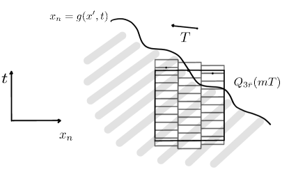
Figure 5. Proof of Theorem 1.3.

References

- [A] Ancona A., Principe de Harnack a la frontiere et theoreme de Fatou pour un operateur elliptique dons un domaine lipschitzien, Ann. Inst. Fourier 28 (1978) 169–213.
- [BBB] Banuelos R., Bass R.F. and Burdzy K., Hölder Domains and The Boundary Harnack Principle, Duke Math. J., 64, 195–200 (1991).
- [BB1] Bass R.F. and Burdzy K., A boundary Harnack principle in twisted Hölder domains, Ann. Math. 134 (1991) 253–276.
- [BB] Bass R.F. and Burdzy K., Lifetimes of conditioned diffusions, Probability Theory and Related Fields volume 91, 405–443(1992).
- [BB2] Bass R.F. and Burdzy K., The boundary Harnack principle for non-divergence form elliptic operators, J. London Math. Soc. (2) 50 (1994), no. 1, 157–169.
- [CFMS] Caffarelli L., Fabes E., Mortola S. and Salsa S., Boundary behavior of non-negative solutions of elliptic operators in divergence form, Indiana Math. J.,30, 621–640 (1981).
- [D] Dahlberg B., On estimates of harmonic measure, Arch. Rational Mech. Anal. 65 (1977), 272–288.
- [DS1] De Silva D., Savin O., A short proof of Boundary Harnack Inequality, Journal of Differential Equations, Volume 269, Issue 3, 15 July 2020, pp. 2419–2429.
- [DS2] De Silva D., Savin O., On Boundary Harnack Inequality in Hölder Domains, to appear in “Partial Differential Equations from theory to applications”, Journal Mathematics in Engineering (in honor of A. Farina).
- [FGMS] Fabes E.B., Garofalo N., Marin-Malave S. and Salsa S., Fatou theorems for some nonlinear elliptic equations, Rev. Mat. Iberoamericana, 4 (1988) 227–252.
- [FGS] Fabes E.B., Garofalo N., and Salsa S., A backward Harnack inequality and Fatou theorem for nonnegative solutions of parabolic equations, Illinois J. Math. 30 (1986), no. 4, 536–565.
- [FSY] Fabes E.B., Safonov M.V., and Yuan Y.,Behavior near the boundary of positive solutions of second order parabolic equations. II, Trans. of AMS Volume 351, Number 12, pp 4947–4961 (1999).
- [F] Ferrari F., On boundary behavior of harmonic functions in Hölder domains, Journal of Fourier Analysis and Applications, 1998, Volume 4, Issue 4-5, pp 447–461 (1988).
- [Fr] Friedman A., Parabolic equations of the second order, Trans. Amer. Math. Soc., 93 (1959), 509–530.
- [G] Garofalo N., Second Order Parabolic Equations in Nonvariational Form: Boundary Harnack Principle and Comparison Theorems for Nonnegativc Solutions, Ann. Mat. Pura Appl. (4) 138 (1984), 267–296.
- [HLN] Hofmann S., Lewis J.L., and Nystrom K., Caloric measure in parabolic flat domains, Duke Math. J. 122 (2004), no. 2, 281–346.
- [JK] Jerison D.S. and Kenig C.E., Boundary Behavior of Harmonic Functions in Non-tangentially Accessible Domains, Adv. Math.,46, 80–147 (1982).
- [K] Kemper J.T., A boundary Harnack principle for Lipschitz domains and the principle of positive singularities, Comm. Pure Appl. Math. 25 (1972), 247–255.
- [K2] Kemper J.T., Temperatures in several variables: Kernel functions, representations, and parabolic boundary values, Trans. Amer. Math. Soc. 167 (1972), 243–262.
- [KiS] Kim H. and Safonov M.V., Boundary Harnack principle for second order elliptic equations with unbounded drift, Problems in mathematical analysis. No. 61. J. Math. Sci. (N.Y.) 179 (2011), no. 1, 127–143.
- [M] Moser J., A harnack inequality for parabolic differential equations, Comm. Pure App. Math 17 (1964), Issue 1, 101–134.
- [PS] Petrosyan A., Shi W., Parabolic Boundary Harnack Principles in Domains with Thin Lipschitz Complement, Anal. PDE 7 (6) (2014), 1421–1463.
- [S] Safonov M.V., Non-divergence elliptic equations of second order with unbounded drift, Nonlinear partial differential equations and related topics, 211–232, Amer. Math. Soc. Transl. Ser. 2, 229, Adv. Math. Sci., 64, Amer. Math. Soc., Providence, RI, 2010.
- [Sal] Salsa S., Some properties of nonnegative solutions of parabolic differential operators, Ann. Mat. Pura Appl. (4) 128 (1981), 193–206.
- [Wa] Wang L., On the regularity theory of fully nonlinear parabolic equations: I Comm. Pure Appl. Math 45 (1992), Issue1, 27–76.
- [W] Wu J.-M. G., Comparison of kernel functions, boundary Harnack principle, and relative Fatou theorem on Lipschitz domains, Ann. Inst. Fourier Grenoble 28 (1978) 147–167.