Quadratic and cubic spherically symmetric black holes in the modified teleparallel equivalent of general relativity: Energy and thermodynamics

Abstract

In Bahamonde et al. (2019), a spherically symmetric black hole (BH) was derived from the quadratic form of $f(T)$. Here we derive the associated energy, invariants of curvature, and torsion of this BH and demonstrate that the higher–order contribution of torsion renders the singularity weaker compared with the Schwarzschild BH of general relativity (GR). Moreover, we calculate the thermodynamic quantities and reveal the effect of the higher–order contribution on these quantities. Therefore, we derive a new spherically symmetric BH from the cubic form of $f(T)=T+\epsilon\Big{[}\frac{1}{2}\alpha T^{2}+\frac{1}{3}\beta T^{3}\Big{]}$, where $\epsilon<<1$, $\alpha$, and $\beta$ are constants. The new BH is characterized by the two constants $\alpha$ and $\beta$ in addition to $\epsilon$. At $\epsilon=0$ we return to GR. We study the physics of these new BH solutions via the same procedure that was applied for the quadratic BH. Moreover, we demonstrate that the contribution of the higher–order torsion, $\frac{1}{2}\alpha T^{2}+\frac{1}{3}\beta T^{3}$, may afford an interesting physics.

I Introduction

The black hole (BH) is the most interesting phenomena in the general relativity (GR) of Einstein and other modified gravitational theories Capozziello and De Laurentis (2011); Clifton et al. (2012); Heisenberg (2019); Stetsko (2020). This profound and sustained interest in the different approaches to BH physics can be investigated because of its relevance in astrophysics Will (2014) and the numerous applications and methods that have initially evolved in the gravitational theories of different systems. Regarding the BH many topics including the horizons global structure, Hawking radiation and thermodynamic properties which are considered as the main goals for realizing the form of the space-time can be studied Carlip (2020). Although GR is a satisfactory gravitational theory, modified theories remain greatly desired. It has been proven that GR is a successful theory for isolated masses with length scales of the solar system; however, this theory still faces disputes in the domains of cosmology and quantum scales.

There are many alternative gravitational theories to GR in the literature and the teleparallel equivalent of general relativity (TEGR), which was applied by Einstein in (1928) to unify gravity and electromagnetism Unzicker and Case (2005) is among these theories. In this theory, the tetrad field is used as a dynamic field instead of the metric of GR. The affine connection is defined regarding the nonsymmetric Weitzenböck connection in the TEGR theory whereas the Live-Civita connection plays the affine connection in GR. The use of the Weitzenböck connection affords a space-time without curvature and the gravitational field is encoded in the torsion tensor, which is the difference between two Weitzenböck connections. The Lagrangian of the TEGR theory depends on the torsion scalar, $T$, which is mainly constructed from the torsion tensor. There are many physical models in the solar system regarding the TEGR theory, as well as in cosmologyde Andrade et al. (2000); Nashed (2018); Aldrovandi et al. (2003); Maluf (2013); Shirafuji et al. (1996); de Andrade and Pereira (1997); El Hanafy and Nashed (2016); Nashed and Capozziello (2019a); Nashed (2006a, 2010, b); NASHED and SHIRAFUJI (2007); ULHOA et al. (2010).

Similar to $f(R)$ which is a generalization of GR in which the Palatini action that depends on the Ricci scalar, $R$, is replaced by an arbitrary analytic differentiable function Capozziello et al. (2011); Nojiri and Odintsov (2011); NOJIRI and ODINTSOV (2007); Nojiri et al. (2017); Nashed and Capozziello (2019b), there is a generalization of the TEGR theory, which is called the $f(T)$ gravitational theory Bengochea (2011); Karami and Abdolmaleki (2013); Dent et al. (2011); Cai et al. (2011); Capozziello et al. (2011). Although TEGR is formulated from a geometry ( Weitzenböck geometry) that is different from GR (the Riemann geometry) both theories are equivalent from the viewpoint of field equations. Nevertheless, when we assume the generic forms of $f(R)$ and $f(T)$, the two theories become inequivalent Mai and Lü (2017); Ferraro and Fiorini (2008); FIORINI and FERRARO (2009). The $f(T)$ theory is an interesting method of solving the challenges of dark energy and dark matters Cardone et al. (2012); Myrzakulov (2011); Yang (2011); Bamba et al. (2013); Camera et al. (2014); Nashed (2015, 2013a); Wang (2011). Moreover, in the frame of $f(T)$ there are many interesting BH and cosmological solutions that have interesting physics Rodrigues et al. (2013); Ferraro and Fiorini (2011); Nashed (2013b); Junior et al. (2015); Iorio and Saridakis (2012); Xie and Deng (2013); Ruggiero and Radicella (2015); Awad et al. (2018, 2017); Chen et al. (2020); Cai et al. (2016). Here we considered the cubic form of the $f(T)$ gravitational theories in the framework of the spherically symmetric space-time to derive a new spherically symmetric BH. Additionally, we reconsidered the BH that was derived in Bahamonde et al. (2019) to calculate its associated energy, invariants of curvature, and torsion, thereby demonstrating and show how the higher-order contribution of torsion.

This study is arranged as follows. In Section II, we briefly reviewed the TEGR and $f(T)$ formalisms. In Section III, we discussed the application of a tetrad field that possesses spherical symmetry in four-dimensions to the vacuum field equations of the $f(T)$ gravity after which the estimated solution of four-dimensions is derived for the quadratic form of $f(T)$ Bahamonde et al. (2019). This BH asymptotically behaves as the flat space-time. The physical properties of this BH were studied by calculating its invariants in Section III.1. In Sections III.2 and III.3 we calculated the energy content and derived the stability condition via the geodesic deviation respectively. In Section IV, we presented the cubic form of the field equation, using $f(T)=T+\epsilon\Big{[}\frac{1}{2}\alpha T^{2}+\frac{1}{3}\beta T^{3}\Big{]}$, and derived a new BH solution, up to $O(\epsilon)$, for these differential equations. In Section V the physical properties of the BH which was derived in the cubic form were discussed and analyzed. In Sections VI.1 and VI.2, we calculated the thermodynamic quantities like, Hawking temperature, entropy, heat capacity and Gibbs energy for the quadratic, and the cubic BH solutions, respectively. The final section was devoted to the discussion and conclusion.

II $f(T)$ theory

Einstein used the TEGR theory, which is a gauge theory Unzicker and Case (2005) to fulfill his dream of unifying gravity with electromagnetism. In this theory, $T$ was responsible for the gravitational field in the same way $R$ was in the Riemann geometry. The affine connection of the TEGR theory (the Weitzenböck connection) is defined by the following connection Weitzenböck (1923)

$${{W^{\lambda}}_{\mu\nu}}:={{e_{i}}^{\lambda}\leavevmode\nobreak\ \partial_{\nu}e^{i}{{}_{\mu}}},$$ (1)

where $e^{i}{{}_{\mu}}$ is the dynamical tetrad in four-dimensions. The metric space-time is defined regardin the tetrad as follows:

$${g_{\mu\nu}:=\eta_{ij}{e^{i}}_{\mu}{e^{j}}_{\nu},}$$ (2)

where $\eta_{ij}=(+,-,-,-)$ is a four-dimensional Minkowskian metric of the tangent space. Using the Weitzenböck connection, the torsion and contortion tensors are defined as follows:

$${T^{\alpha}}_{\mu\nu} := {W^{\alpha}}_{\nu\mu}-{W^{\alpha}}_{\mu\nu}={e_{i}}^{\alpha}\left(\partial_{\mu}{e^{i}}_{\nu}-\partial_{\nu}{e^{i}}_{\mu}\right),$$

$${\gamma^{\mu\nu}}_{\alpha} := -\frac{1}{2}\left({T^{\mu\nu}}_{\alpha}-{T^{\nu\mu}}_{\alpha}-{T_{\alpha}}^{\mu\nu}\right).$$ (3)

It is well known that the difference between Weitzenböck and Levi-Civita connections reproduces the contortion, as follows:

$${\gamma^{\mu}}_{\nu\alpha}={W^{\mu}}_{\nu\alpha}-{\Gamma^{\mu}}_{\nu\alpha}.$$ (4)

The superpotential tensor ${\Sigma_{\mu}}^{\nu\alpha}$ which is the antisymmetric tensor in the last two indices is defined as follows:

$${\Sigma_{\alpha}}^{\mu\nu}:=\frac{1}{2}\left({\gamma^{\mu\nu}}_{\alpha}+\delta^{\mu}_{\alpha}{T^{\beta\nu}}_{\beta}-\delta^{\nu}_{\alpha}{T^{\beta\mu}}_{\beta}\right).$$ (5)

Using all the above data we can define $T$ of the TEGR theory according to Eq. (6):

$$T:={T^{\alpha}}_{\mu\nu}{\Sigma_{\alpha}}^{\mu\nu},$$ (6)

Similar to the GR extension ($f(R)$) it was logical to modify the TEGR theory to include higher torsion orders, which enabled us to define the Lagrangian of $f(T)$, where $f$ is an analytical continues differentiable function of $T$:

$${\mathcal{L}}=\frac{1}{2\kappa}\int|e|f(T)\leavevmode\nobreak\ d^{4}x,$$ (7)

where $|e|=\sqrt{-g}=\det\left({e^{a}}_{\mu}\right)$ is the determinate of the metric and $\kappa$ is a four-dimensional constant that is defined as $\kappa=\frac{8\pi G}{c^{4}}$, where $G$ is the Newtonian gravitational constant in four-dimensions and $c$ is the speed of light. The variation of Eq. (7) w.r.t. the tetrad field, ${e^{i}}_{\mu}$ affords the following field equations of $f(T)$ in the vacuum case as shown in Bengochea (2011):

$${S_{\mu}}^{\rho\nu}\partial_{\rho}Tf_{TT}+\left[e^{-1}{e^{i}}_{\mu}\partial_{\rho}\left(e{e_{i}}^{\alpha}{S_{\alpha}}^{\rho\nu}\right)-{T^{\alpha}}_{\lambda\mu}{S_{\alpha}}^{\nu\lambda}\right]f_{T}-\frac{f}{4}\delta^{\nu}_{\mu}=\mathfrak{\xi}^{\nu}{}_{\mu}\equiv 0,$$ (8)

where $f:=f(T)$,    $f_{T}:=\frac{\partial f(T)}{\partial T}$ and $f_{TT}:=\frac{\partial^{2}f(T)}{\partial T^{2}}$. The application of the field equations (8) to a spherically symmetric tetrad field using the form of $f(T)=T+\epsilon\Big{[}\frac{1}{2}\alpha T^{2}+\frac{1}{3}\beta T^{3}\Big{]}$ is shown in Section IV.

III Asymptotically stationary AdS black holes

In this section, the field equations of the higher order torsion theory, (Eq. (8)) were applied to the spherically symmetric space-time, thus affording the vielbein which is written in the spherical coordinate ($t$, $r$, $\theta$, $\phi$) as shown in Bahamonde et al. (2019):

$$e^{a}{}_{\nu}=\left(\begin{array}[]{cccc}\sqrt{\mu}&0&0&0\\ 0&\sqrt{\nu}\cos(\phi)\sin(\theta)&r\cos(\phi)\cos(\theta)&-r\sin(\phi)\sin(\theta)\\ 0&\sqrt{\nu}\sin(\phi)\sin(\theta)&r\sin(\phi)\cos(\theta)&r\cos(\phi)\sin(\theta)\\ 0&\sqrt{\nu}\cos(\theta)&-r\sin(\theta)&0\\ \end{array}\right)\,.$$ (9)

where $-\infty<t<\infty$, $0\leq r<\infty$, $0\leq\theta<\pi$, $0\leq\phi<2\pi$, $\mu$ and $\nu$ are the two unknown functions of $r$. Thus, the space-time, which can be generated by (9) is expressed as follows:

$$ds^{2}=\mu(r)\,dt^{2}-\nu(r)\,dr^{2}-r^{2}d\Sigma^{2}\,,$$ (10)

where $d\Sigma^{2}=d\theta^{2}+\sin^{2}\theta d\phi^{2}$ is the two dimensional sphere. Substituting Eq. (9) into Eq. (6), we evaluate $T$ as follows

$$T=-\frac{2\left(\sqrt{\nu(r)}-1\right)\left(r\mu^{\prime}(r)-\mu(r)\sqrt{\nu(r)}+\mu(r)\right)}{r^{2}\mu(r)\nu(r)}\,..$$ (11)

Applying Eq. (9) to the vacuum field equation (8) the following nonvanishing components could be obtained Bahamonde et al. (2019):

$$\xi^{t}{}_{t} = \frac{r\beta(\sqrt{\nu}-1)\mu^{\prime}+\mu(r\nu^{\prime}+2\nu^{3/2}-2\nu)}{2r^{2}\mu\nu^{2}}f_{T}+\frac{(\sqrt{\nu}-1)}{r\nu}T^{\prime}f_{TT}+\frac{1}{4}f\,,$$ (12)

$$\xi^{r}{}_{r} = -\frac{r(\sqrt{\nu}-2)\mu^{\prime}+2\mu(\sqrt{\nu}-1)}{2r^{2}\mu\nu}f_{T}-\frac{1}{4}f\,,$$ (13)

$$\xi^{\theta}{}_{\theta}=\xi^{\phi}{}_{\phi} = \frac{-r^{2}\nu\mu^{\prime 2}+r\nu\left(-r\mu^{\prime}\nu^{\prime}-4\nu^{3/2}\mu^{\prime}+2\nu\left(r\mu^{\prime\prime}+3\mu^{\prime}\right)\right)+\mu^{2}\left(-2r\nu^{\prime}-8\nu^{3/2}+4\nu^{2}+4\nu\right)}{8r^{2}\mu^{2}\nu^{2}}f_{T}$$ (14)

$$+\frac{r\mu^{\prime}-2\mu(\sqrt{\nu}-1)}{4r\mu(r)\nu(r)}T^{\prime}f_{TT}-\frac{1}{4}f\,,$$

Bahamonde et al. Bahamonde et al. (2019) have solved the above system when $f(T)=T+\frac{1}{2}\epsilon\,\alpha T^{p}$. In this section, we discussed the physics of the BH solution that was derived in Bahamonde et al. (2019) for the case “p=2”:

$$\mu(r)=\sigma+\epsilon\,\sigma_{1}\,,\qquad\qquad\nu(r)=\sigma^{-1}+\epsilon\,\sigma_{2}\,,$$ (15)

where

$$\sigma = 1-\frac{2m}{r}\,,$$

$$\sigma_{1} = \left[-\frac{c_{1}}{r}+c_{2}-\alpha\left(\frac{m^{2}+6mr+r^{2}}{mr^{3}}-\frac{16\left(1-\frac{2m}{r}\right)^{3/2}}{3m^{2}}+\frac{(1-\frac{3m}{r})}{2m^{2}}\ln\left(1-\frac{2m}{r}\right)\right)\right]\,,$$

$$\sigma_{2} = \left[\frac{\left(\frac{c_{1}}{r}-\frac{2c_{2}m}{r}\right)}{\left(1-\frac{2m}{r}\right)^{2}}-\alpha\left(-\frac{8(3m^{2}-7mr+2r^{2})}{3mr^{3}(1-\frac{2m}{r})^{3/2}}+\frac{25m-23r}{r^{3}(1-\frac{2m}{r})^{2}}+\frac{\ln\left(1-\frac{2m}{r}\right)}{2mr(1-\frac{2m}{r})^{2}}\right)\right]\,,$$ (16)

with $c_{1}$ and $c_{2}$ are the constants of the integration. Equation (15) could be reduced to the Schwarzschild BH GR when $\epsilon=0$. In the following subsections we extracted the physics of Eq. (15) when $\epsilon\neq 0$. From now on we will refer to solution (15) as “p=2”.

III.1 Singularities of “p=2”

We calculate the invariant of Eq. (15), up to $O(\epsilon)$, and obtained the following

$$T^{\mu\nu\lambda}T_{\mu\nu\lambda}=-\frac{16\epsilon\,m}{r^{2}}+\frac{2m^{2}}{r^{4}}$$

$$+\epsilon\Bigg{[}\frac{8c_{1}+12\alpha ln(2)/m+128\alpha/3m-16mc_{2}}{r^{3}}+\frac{2mc_{1}+3\alpha ln(2)+32\alpha/3-4m^{2}c_{2}}{r^{4}}\Bigg{]}+O\Big{(}\frac{1}{r^{6}}\Big{)},$$

$$T^{\mu}T_{\mu}=-\frac{16\epsilon\,m}{r^{2}}-\frac{m^{2}}{r^{4}}-\frac{4m^{3}}{r^{5}}+\epsilon\Bigg{[}\frac{64\alpha/3m-8mc_{2}+6\alpha ln(2)/m+4c_{1}}{r^{3}}$$

$$+\frac{2m^{2}c_{2}-16\alpha/3-3\alpha ln(2)/2-mc_{1}}{r^{4}}+\frac{12m^{3}c_{2}-32m\alpha-9m\alpha ln(2)-6m^{2}c_{1}}{r^{5}}\Bigg{]}+O\Big{(}\frac{1}{r^{6}}\Big{)},$$

$$T(r)=\frac{8\epsilon\,m}{r^{2}}+\frac{2m^{2}}{r^{4}}+\frac{4m^{3}}{r^{5}}+\epsilon\Bigg{[}\frac{3\alpha\,ln(2)+2m\,c_{1}+32\alpha/3-4m^{2}\,c_{2}}{r^{4}}+\frac{9m\,\alpha\,ln(2)+6\,m^{2}\,c_{1}+32\,m\,\alpha-12\,m^{3}\,c_{2}}{r^{5}}\Bigg{]}+O\Big{(}\frac{1}{r^{6}}\Big{)},$$

$$R^{\mu\nu\lambda\rho}R_{\mu\nu\lambda\rho}=-\frac{48m^{2}}{r^{6}}+\epsilon\Bigg{[}\frac{96m^{2}c_{2}-48mc_{1}-256\alpha-72\alpha ln(2)}{r^{6}}\Bigg{]}+O\Big{(}\frac{1}{r^{10}}\Big{)},$$

$$R^{\mu\nu}R_{\mu\nu}=O\Big{(}\epsilon^{2}\Big{)}\,,\qquad R=\epsilon\Bigg{[}\frac{16m^{3}\alpha}{r^{7}}+\frac{20m^{4}\alpha}{r^{8}}\Bigg{]}+O\Big{(}\frac{1}{r^{9}}\Big{)},$$ (17)

where $T^{\mu\nu\lambda}T_{\mu\nu\lambda}$ $T^{\mu}T_{\mu}$, $T$, $R^{\mu\nu\lambda\rho}R_{\mu\nu\lambda\rho}$, $R^{\mu\nu}R_{\mu\nu}$ and $R$, are the torsion tensor square, torsion vector square, torsion scalar, Kretschmann scalar, Ricci tensor square, and Ricci scalar. The above invariants indicated that there was a singularity (curvature singularity) at $r=0$. Close to $r=0$, the behaviors of $T^{\mu\nu\lambda}T_{\mu\nu\lambda}$, $T^{\mu}T_{\mu}$, $T$ are given by $T^{\alpha\beta\gamma}T_{\alpha\beta\gamma}=T^{\alpha}T_{\alpha}=T\sim{r^{-2}}$ in contrast with the solutions of the Einstein theory in GR and TEGR, which are given as $T^{\alpha\beta\gamma}T_{\alpha\beta\gamma}=T^{\alpha}T_{\alpha}=T\sim{r^{-4}}$. This demonstrates that the singularity of the higher-order torsion theory was much milder than the one obtained in GR and TEGR for the natural spherically symmetric case. This result suggests that these singularities are weak ones, according to Tipler and Krolak Clarke and Królak (1985); Tipler (1977), and the possibility of extending the geodesics beyond these regions. This would be discussed in subsequent studies.

III.2 Energy content of “p=2”

Here, we calculated the energy content of Eq. (15). To do this, we applied the Hamiltonian density $H$ which can be obtained from the Lagrangian equation $(\ref{q7})$ by rewriting it as follows:

$${\mathcal{L}}=p\dot{q}-H.$$

The Hamiltonian of the $f(T)$ gravitational theory is expressed as follows:

$$H=e^{a}{}_{0}B^{a}+\xi_{ij}\Gamma^{ij}+\xi_{j}\Gamma^{j},\qquad\xi_{ij}=\frac{1}{2}e_{i}{}^{\alpha}e_{j}{}^{\beta}(T_{\alpha 0\beta}-T_{\beta 0\alpha}),\qquad\xi_{j}=e_{0}{}^{\alpha}e_{j}{}^{\beta}T_{\alpha 0\beta},$$ (18)

where $\xi_{ij}$ and $\xi_{j}$ are the Lagrange multipliers. The components $e^{a}{}_{0}$ do not exhibit time dependence thus this quantity could be considered as a Lagrange multiplier. The canonically conjugate moneta to $e^{a}{}_{\alpha}$ are denoted by $\Pi^{a\alpha}$. In the configuration space one can obtain ULHOA and SPANIOL (2013):

$$\Pi^{ac}=e^{a}{}_{\alpha}e^{c}{}_{\beta}\Pi^{\alpha\beta}=-4\pi e^{a}{}_{\alpha}e^{c}{}_{\beta}\Sigma^{\alpha 0\beta}f_{T}=-4\pi\Sigma^{a0c}f_{T}.$$ (19)

Therefore, writing $H$ in terms of $e^{a}_{\alpha}$, $\Pi^{a\alpha}$ and Lagrange multipliers is possible. To express a simple form of $H$ some Lagrange multipliers and constraints were redefined Maluf et al. (2006) and Eq. (18) reads as follows:

$$H=e_{a0}C^{a}+\frac{1}{2}\lambda_{ab}\Gamma^{ab},$$ (20)

where $e_{a0}$ and $\lambda_{ab}=-\lambda_{ba}$ are the Lagrange multipliers, and $C^{a}$ and $\Gamma^{ab}$ are the first-class constraints. Solving the Hamilton field equations can aid the identifications of $\lambda_{ij}=e_{i}{}^{\alpha}e_{j}{}^{\beta}\lambda_{\alpha\beta}=\frac{1}{2}e_{i}{}^{\alpha}e_{j}{}^{\beta}(T_{\alpha 0\beta}-T_{\beta 0\alpha})$ and $\lambda_{0j}=e_{0}{}^{\alpha}e_{j}{}^{\beta}\lambda_{\alpha\beta}=e_{0}{}^{\alpha}e_{j}{}^{\beta}T_{\alpha 0\beta}$. The quantities $\lambda_{ij}$ and $\lambda_{0j}$ are the components of Eq. (21)

$$\lambda_{\mu\nu}=e^{a}{}_{\mu}e^{b}{}_{\nu}\lambda_{ab}.$$ (21)

The constraint $C^{a}$ may be written in the following form:

$$C^{a}=-\partial_{i}\Pi^{ai}f_{T}+f^{a},$$ (22)

where $f^{a}$ is a lengthy expression of the field quantities. Notably $\partial_{i}\Pi^{ai}$ is the only total divergence term of the momenta $\Pi^{ai}$, which emerged in the expression of $C^{a}$. The constraint $C^{a}=0$ inspired the definition of the gravitational energy-momentum $P^{a}$ in four-dimensions in the integral form:

$$P^{a}=-\int_{V}d^{3}x\partial_{i}\Pi^{ai},$$ (23)

where $V$ is the three-dimensional volume of the space ULHOA and SPANIOL (2013).

Next the energy that was related to the BH was calculated using Eq. (15). Using Eq. (23), the necessary components for calculating the energy in the following form could be derived:

$$\Sigma^{(0)(0)1}=\frac{r\sin(\theta)\sqrt{\mu\nu}(\sqrt{\nu}-1)}{\nu}.$$ (24)

Substituting Eqs. (15) and (24) into Eq. (23), we obtained the energy content of the black hole (15), up to $O(\epsilon)$, in the following form:

$$P^{0}=E\approx m+\epsilon\frac{44\alpha+24mc_{1}+3\alpha ln(2)-4m^{2}c_{2}}{8m}+O\left(\frac{1}{r}\right),$$

which obtained $E=m$ when $\epsilon\rightarrow 0$ which is ADM (Arnowitt, Deser Misner) mass Misner et al. (1973). Equation (III.2) is finite value and indicates that the energy depended on the coefficient of the higher-order torsion terms, $\epsilon$, up to order O$\left(\frac{1}{r}\right)$. Moreover, Eq. (23) indicates that the values of $\epsilon$, $\alpha$ and $c_{1}$ must be positive and that of $c_{2}$ must be negative value or $8m^{2}+\epsilon(44\alpha+24mc_{1}+3\alpha ln(2))>4\epsilon m^{2}c_{2}$.

III.3 Analysis of the stability of the black hole with the geodesic deviation

The paths of a test particle in the gravitational field are described by the following equation:

$${d^{2}x^{\alpha}\over d\tau^{2}}+\Bigl{\{}^{\alpha}_{\beta\rho}\Bigr{\}}{dx^{\beta}\over d\tau}{dx^{\rho}\over d\tau}=0,$$ (26)

which is known as the geodesic equations. In Eq. (26) $\tau$ represents the affine connection parameter. The geodesic deviation possesses the form D’Inverno (1992); Nashed (2003)

$${d^{2}\xi^{\sigma}\over d\tau^{2}}+2\Bigl{\{}^{\sigma}_{\mu\nu}\Bigr{\}}{dx^{\mu}\over d\tau}{d\xi^{\nu}\over d\tau}+\Bigl{\{}^{\sigma}_{\mu\nu}\Bigr{\}}_{,\ \rho}{dx^{\mu}\over d\tau}{dx^{\nu}\over d\tau}\xi^{\rho}=0,$$ (27)

where $\xi^{\rho}$ is the four-vector deviation. Introducing (15) into (26) and (27), obtained the following:

$${d^{2}t\over d\tau^{2}}=0,\qquad{1\over 2}\mu^{\prime}(r)\left({dt\over d\tau}\right)^{2}-r\left({d\phi\over d\tau}\right)^{2}=0,\qquad{d^{2}\theta\over d\tau^{2}}=0,\qquad{d^{2}\phi\over d\tau^{2}}=0,$$ (28)

and for the BH regarding the geodesic deviation (15) afforded the following:

$${d^{2}\xi^{1}\over d\tau^{2}}+\nu(r)\mu^{\prime}(r){dt\over d\tau}{d\xi^{0}\over d\tau}-2r\nu(r){d\phi\over d\tau}{d\xi^{3}\over d\tau}+\left[{1\over 2}\left(\mu^{\prime}(r)\nu^{\prime}(r)+\nu(r)\mu^{\prime\prime}(r)\right)\left({dt\over d\tau}\right)^{2}-\left(\nu(r)+r\nu^{\prime}(r)\right)\left({d\phi\over d\tau}\right)^{2}\right]\xi^{1}=0,$$

$${d^{2}\xi^{0}\over d\tau^{2}}+{\nu^{\prime}(r)\over\nu(r)}{dt\over d\tau}{d\zeta^{1}\over d\tau}=0,\qquad{d^{2}\xi^{2}\over d\tau^{2}}+\left({d\phi\over d\tau}\right)^{2}\xi^{2}=0,\qquad\qquad{d^{2}\xi^{3}\over d\tau^{2}}+{2\over r}{d\phi\over d\tau}{d\xi^{1}\over d\tau}=0,$$ (29)

where $\mu(r)$ and $\nu(r)$ were defined from Eq. (15), $\nu^{\prime}(r)=\displaystyle{d\alpha(r)\over dr}$. Using the circular orbit

$$\theta={\pi\over 2},\qquad{d\theta\over d\tau}=0,\qquad{dr\over d\tau}=0,$$ (30)

we get

$$\left({d\phi\over d\tau}\right)^{2}={\mu^{\prime}(r)\over r[2\mu(r)-r\mu^{\prime}(r)]},\qquad\left({dt\over d\tau}\right)^{2}={2\over 2\mu(r)-r\mu^{\prime}(r)}.$$ (31)

Further, Eqs. (III.3) can be rewritten as follows:

$${d^{2}\xi^{1}\over d\phi^{2}}+\mu(r)\mu^{\prime}(r){dt\over d\phi}{d\xi^{0}\over d\phi}-2r\mu(r){d\xi^{3}\over d\phi}+\left[{1\over 2}\left[\mu^{\prime 2}(r)+\mu(r)\mu^{\prime\prime}(r)\right]\left({dt\over d\phi}\right)^{2}-\left[\mu(r)+r\mu^{\prime}(r)\right]\right]\zeta^{1}=0,$$

$${d^{2}\xi^{2}\over d\phi^{2}}+\xi^{2}=0,\qquad{d^{2}\xi^{0}\over d\phi^{2}}+{\mu^{\prime}(r)\over\mu(r)}{dt\over d\phi}{d\xi^{1}\over d\phi}=0,\qquad{d^{2}\xi^{3}\over d\phi^{2}}+{2\over r}{d\xi^{1}\over d\phi}=0.$$ (32)

The second equation of Eq. (III.3) corresponds to a simple harmonic motion, which indicates the stability on the plane $\theta=\pi/2$, assuming the remaining equations of (III.3) obtained solutions in the form of Eq. (33):

$$\xi^{0}=\zeta_{1}e^{i\sigma\varphi},\qquad\xi^{1}=\zeta_{2}e^{i\sigma\varphi},\qquad and\qquad\xi^{3}=\zeta_{3}e^{i\sigma\varphi},$$ (33)

where $\zeta_{1},\zeta_{2}$ and $\zeta_{3}$ are the constants and $\varphi$ is an unknown variable. Substituting Eq. (33) into (III.3), the stability condition for static spherically symmetric charged BH can be obtained in the following form:

$$\frac{3\mu\nu\nu^{\prime}-\sigma^{2}\mu\nu^{\prime}-2r\nu^{3/2}\mu^{\prime 3/2}-r\mu\nu^{\prime 2}+r\mu\nu^{\prime}\mu^{\prime}+r\mu\nu\mu^{\prime\prime}}{\mu\nu^{\prime}}>0.$$ (34)

Equation (34) obtained the following solution:

$$\sigma^{2}=\frac{3\mu\nu\nu^{\prime}-2r\nu^{3/2}\mu^{\prime 3/2}-r\mu\nu^{\prime 2}+r\mu\nu^{\prime}\mu^{\prime}+r\mu\nu\mu^{\prime\prime}}{\mu^{2}\nu^{\prime 2}}>0.$$ (35)

Figure 1 which exhibits the regions where the BH solutions are stable and the regions where there are no possible stability is a plot of Eq. (35) for particular values of the model.

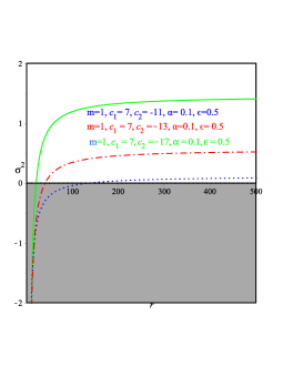
(a)  Stability of (35)

Figure 1: Schematic plot of Eq. (35), namely, $\sigma^{2}$ versus the coordinate, $r$.

IV Cubic solution of Eq. (8)

In this section, we derived a novel spherically symmetric solution using the form $f(T)=T+\epsilon\,[\frac{1}{2}\alpha T^{2}+\frac{1}{3}\beta T^{3}]$. To do this, we are derived the cubic form of the field equations (8) as follows:

$$\xi^{t}{}_{t}=\frac{1}{3r^{6}\varrho^{2}}\Bigg{[}3r^{4}\varrho^{2}(1-\varrho-r\varrho^{\prime})+\epsilon\Big{\{}12r^{2}\varrho^{\prime\prime}\Big{[}\varrho^{5/2}(16\beta-12r\beta\varrho^{\prime}+2r^{2}\alpha)+4\varrho^{3/2}r\beta\varrho^{\prime}+16\varrho^{7/2}\beta-\varrho^{2}(4r\beta\varrho^{\prime}[3+\varrho]$$

$$+4\beta\varrho^{2}+\varrho[24\beta+r^{2}\alpha]+4\beta+r^{2}\alpha)\Big{]}+6r\varrho^{\prime}\Big{[}6\varrho^{5/2}(r^{2}\alpha-4\beta)-24\varrho^{7/2}\beta+\varrho^{2}(6\beta-3r^{2}\alpha+\varrho\{r^{4}\mu_{1}-3r^{2}\alpha$$

$$+36\beta\}+6\varrho^{2}\beta)\Big{]}+3r^{2}\varrho^{\prime 2}[r^{2}\alpha\varrho-48\beta\varrho^{2}-3r^{2}\alpha\varrho^{2}+4\beta\varrho-2[4\beta+r^{2}\alpha+28\varrho\beta]\varrho^{3/2}-20\beta\varrho^{3}]+3r^{3}\beta\varrho^{1/2}\varrho^{\prime 3}\Big{[}3\varrho^{1/2}-4$$

$$+6\varrho-5\varrho^{3/2}\Big{]}+\varrho^{2}\Big{[}3r^{2}\alpha-24[4\beta+r^{2}\alpha]\varrho^{1/2}+6\varrho(70\beta+9r^{2}\alpha)-8\varrho^{3/2}(6r^{2}\alpha+100\beta)+3\varrho^{2}\Big{(}260\beta+r^{5}\nu^{\prime}_{1}$$

$$+\nu_{1}r^{4}+5r^{2}\alpha\Big{)}+\beta\varrho^{5/2}(76\varrho^{1/2}-384)\Big{]}\Big{\}}\Bigg{]}\,,$$

$$\xi^{r}{}_{r}=\frac{1}{3r^{6}\varrho^{3/2}}\Bigg{[}3r^{4}\varrho^{3/2}(1-\varrho-r\varrho^{\prime})+\epsilon\Big{\{}3r\varrho^{\prime}\Big{[}\varrho^{5/2}\{r^{4}\nu_{1}-6(r^{2}\alpha+20\beta)\}-2\varrho^{3/2}(10\beta+3r^{2}\alpha)-20\varrho^{7/2}\beta+r^{4}\mu_{1}\varrho^{1/2}$$

$$+80\beta\varrho^{3}+4\varrho^{2}\{20\beta+3r^{2}\alpha\}\Big{]}-3r^{2}\varrho^{\prime 2}\Big{[}(72\beta+20\varrho+3r^{2}\alpha)\varrho^{3/2}-\varrho^{1/2}(32\varrho^{1/2}\beta+4r^{2}\alpha\varrho^{1/2}+4\beta+r^{2}\alpha-64\beta\varrho^{3/2})\Big{]}$$

$$+4r^{3}\beta\varrho^{\prime 3}\Big{[}2+12\varrho-\varrho^{1/2}(9+5\varrho)\Big{]}+\varrho^{3/2}\Big{[}3r^{2}\alpha+4\beta-3r^{5}\mu^{\prime}_{1}-6\varrho(3r^{2}\alpha-10\beta)+8\varrho^{3/2}(3r^{2}\alpha+20\beta)-3\varrho^{2}\Big{(}60\beta+3r^{2}\alpha$$

$$-r^{4}\nu_{1}\Big{)}-4\beta\varrho^{5/2}(24-5\varrho^{1/2})\Big{]}\Big{\}}\Bigg{]}\,,$$

$$\xi^{\theta}{}_{\theta}=\xi^{\phi}{}_{\phi}=\frac{1}{12r^{6}\varrho^{2}}\Bigg{[}6r^{5}\varrho^{2}(2\varrho^{\prime}+r\varrho^{\prime\prime})-\epsilon\Big{\{}6r^{2}\varrho^{\prime\prime}\Big{[}4r\varrho^{3/2}\varrho^{\prime}(r^{2}\alpha+8\beta+6r\beta\varrho^{\prime})+4\varrho^{5/2}(20\beta+3r^{2}\alpha+24r\beta\varrho^{\prime})+80\varrho^{7/2}\beta$$

$$+\varrho\Big{(}r^{4}\mu_{1}-2\varrho\{3r^{2}\alpha-10\beta\}+\varrho^{2}\{r^{4}\nu_{1}-6r^{2}\alpha-120\beta\}-20\beta\varrho^{3}-4r\varrho\varrho^{\prime}\{r^{2}\alpha+24\beta+8\beta\varrho\}-12r^{2}\beta\varrho^{\prime 2}\{1+\varrho\}\Big{)}\Big{]}$$

$$+3r\varrho^{\prime}\Big{[}8\varrho^{3/2}(r^{2}\alpha+4\beta)+24r^{2}\varrho^{5/2}\alpha-160\beta\varrho^{7/2}+\varrho\Big{(}2r^{4}\mu_{1}-8\varrho\{3r^{2}\alpha-10\beta\}+2\varrho^{2}\{3r^{4}\nu_{1}-4r^{2}\alpha+80\beta\}$$

$$+48\beta\varrho^{3}+r^{5}\varrho^{2}\nu^{\prime}_{1}+r^{5}\mu^{\prime}_{1}\Big{)}\Big{]}+3r\varrho^{\prime 2}\Big{[}4\varrho^{3/2}(3r^{2}\alpha+20\beta)+112\beta\varrho^{5/2}+32\beta\varrho^{3}+\varrho^{2}(12r^{2}\alpha-r^{4}\nu_{1}+144\beta)+16\varrho\beta+r^{4}\mu_{1}\Big{]}$$

$$+2r^{3}\varrho^{1/2}\varrho^{\prime 3}\Big{[}60\varrho\beta-3r^{2}\alpha-40\varrho^{3/2}\beta-20\beta\Big{]}+24r^{4}\beta\varrho^{\prime 4}\Big{[}1-\varrho^{1/2}\Big{]}-2\varrho^{2}\Big{[}6r^{2}\alpha+16\beta-12\varrho(3r^{2}\alpha+20\beta)$$

$$+16\varrho^{3/2}(40\beta+3r^{2}\alpha)-\varrho^{2}(720\beta+3r^{5}\nu^{\prime}_{1}+18r^{2}\alpha)-16\beta\varrho^{5/2}(5\varrho^{1/2}-24)\Big{]}\Big{\}}\Bigg{]}\,,$$ (36)

where $\varrho=1-\frac{2M}{r}$ and we have used

$$\mu=\varrho+\epsilon\mu_{1},\qquad\textrm{and}\qquad\nu=\varrho^{-1}+\epsilon\nu_{1}.$$ (37)

From the second equation of Eq. (36) we obtained the following expression:

$$\nu_{1}=\frac{1}{3r^{7/2}\varrho^{5/2}}\Big{[}\varrho^{1/2}[3r^{5}\varrho\mu^{\prime}_{1}+3\varrho^{2}(\alpha r^{2}+16\beta)+\varrho(3\mu_{1}r^{4}+18\alpha r^{2}+160\beta)+48\beta+3\alpha r^{2}-3\mu_{1}r^{4}]-4(1+\varrho)(2\beta\varrho^{2}$$

$$+\varrho[3\alpha r^{2}+28\beta]+2\beta)\Big{]}\,.$$ (38)

Further, using Eq. (IV) in the third equation of (36) we obtained the following expression:

$$\mu_{1}=\frac{1}{1890r^{4}\varrho(1-\varrho)^{4}}\Big{[}10r^{2}\varrho^{4}\{189r^{2}c_{4}\varrho+5859\alpha\}+10\beta\varrho^{1/2}[1008-4032\varrho-112\varrho^{6}+34608\varrho^{2}+448\varrho^{5}]$$

$$-10r^{2}\alpha\varrho[945\varrho ln(\varrho)-1323\varrho^{2}ln(\varrho)+567\varrho^{3}ln(\varrho)-189ln(\varrho)+567ln(2)-1134ln(2)\varrho+567ln(2)\varrho^{2}]$$

$$-\beta\varrho\Big{[}105840ln(2)+105840ln(\varrho)\varrho-15120ln(\varrho)+150528\varrho^{5/2}\Big{]}+10c_{4}r^{4}\varrho[189-756\varrho+1134\varrho^{2}-756\varrho^{3}]$$

$$+10c_{3}r^{3}\varrho[756r\varrho^{3}-189+756\varrho-1134\varrho^{2}-189\varrho^{4}]-16065r^{2}\alpha r^{2}\varrho-10\beta\varrho[3318\varrho^{4}+2562+2226\varrho-504\varrho^{2}$$

$$-7224\varrho^{3}]+\alpha\varrho^{2}r^{2}[61425-88830\varrho-16065\varrho^{3}+945\varrho^{4}]+3780\beta\varrho^{6}$$

$$+27936\beta\varrho^{9/2}+10r^{2}\alpha\varrho^{5/2}\{4032\varrho^{2}-8064\varrho+4032\}\Big{]}\,.$$ (39)

Substituting Eq. (39) in Eq. (38) we get the following:

$$\nu_{1}=\frac{1}{1890r^{4}\varrho^{5/2}(1-\varrho)^{4}}\Big{[}9450c_{4}r^{4}\varrho^{3/2}\{1-\varrho^{3}\}+10c_{3}r^{2}\varrho^{3/2}[189r\varrho^{3}-756r\varrho^{2}-756r]+10\varrho^{3/2}[31752\varrho\beta ln(\varrho)-4158r^{2}\alpha]$$

$$+r^{2}\alpha\varrho^{1/2}[5670\varrho^{3}ln(2)-3780\varrho^{2}ln(\varrho)-5670\varrho^{2}ln(2)+17955]-10\beta\varrho^{1/2}[1512ln(\varrho)-10584ln(2)]+1890r^{3}\varrho^{1/2}[c_{3}-rc_{4}]$$

$$+10\alpha r^{2}\varrho^{1/2}[2520\varrho^{7/2}+567ln(2)-189ln(\varrho)]-10\beta[1512-5586\varrho^{1/2}-7896\varrho^{3/2}-1890\varrho^{13/2}-12978\varrho^{5/2}+37506\varrho^{9/2}$$

$$-7560\varrho^{11/2}-27552\varrho^{7/2}]+11340r^{3}\varrho^{5/2}c_{3}+18900r^{4}c_{4}\varrho^{5/2}[\varrho-1]+r^{2}\alpha\varrho^{1/2}[18900\varrho^{5}+5670\varrho^{4}ln(\varrho)+7560\varrho ln(\varrho)$$

$$-5670\varrho ln(2)+945\varrho^{6}-7560\varrho^{3}ln(\varrho)-7560\varrho^{1/2}]+\beta\varrho[108272\varrho^{4}-45360-28560\varrho-1023792\varrho^{2}+287568\varrho^{3}]$$

$$+r^{2}\alpha\varrho^{2}\{25200\varrho-17640-17640\varrho^{3}-7560\varrho^{4}-74655\varrho^{5/2}+83160\varrho^{3/2}-4725\varrho^{1/2}\}+10\beta\varrho^{3/2}\{6048ln(\varrho)+31752ln(2)$$

$$-6776\varrho^{9/2}-168\varrho^{11/2}\}+1890r^{4}c_{4}\varrho^{11/2}\Big{]}\,.$$ (40)

From Eqs. (39) and (40) we constructed the unknown functions $\mu$ and $\nu$ in the asymptotic form up to $O(\epsilon)$. Notably, the metric potential (37) using Eq. (39) and (40) was the solution to the field equations (8) up to $O(\epsilon)$ for the form $f(T)=T+\epsilon\Big{[}\frac{1}{2}\alpha T^{2}+\frac{1}{3}\beta T^{3}\Big{]}$. In Section V we extracted the physics of the solution of (37) using Eqs. (39) and (40).

V Main features of the cubic solution

Some features of the solution that was derived in the previous section were analyzed here.
The asymptote of the metric:
By constructing the metric of solution (37) from Eqs. (39) and (40) we could easily demonstrate that this solution asymptotically behaved as a flat space-time and that is an acceptable behavior.

V.1 Singularities of the cubic solution

We calculated the invariant of solution (37) from Eqs. (39) and (40) and obtained the following:

$$T^{\mu\nu\lambda}T_{\mu\nu\lambda}=-\frac{16\epsilon\,M}{r^{2}}+\frac{-45360M^{4}+\epsilon[M^{3}(15120c_{3}-30240Mc_{4})+\alpha M^{2}(80640+22680ln(2))+\beta(105840ln(2)+32768)]}{7560M^{2}r^{4}}$$

$$+O\Big{(}\frac{1}{r^{5}}\Big{)},$$

$$T^{\mu}T_{\mu}=-\frac{16\epsilon\,M}{r^{2}}+\frac{-5040M^{4}+\epsilon[M^{3}(15120c_{3}-30240Mc_{4})+\alpha M^{2}(80640+22680ln(2))+\beta(105840ln(2)+32768)]}{5040M^{2}r^{4}}$$

$$+O\Big{(}\frac{1}{r^{5}}\Big{)},$$

$$T(r)=\frac{8\epsilon\,M}{r^{2}}+\frac{-15120M^{4}-\epsilon[M^{3}(15120c_{3}-30240Mc_{4})+\alpha M^{2}(80640+22680ln(2))+\beta(105840ln(2)+32768)]}{7560M^{2}r^{4}}$$

$$+O\Big{(}\frac{1}{r^{5}}\Big{)},$$

$$R^{\mu\nu\lambda\rho}R_{\mu\nu\lambda\rho}=-\frac{48M^{2}}{r^{6}}+8\epsilon\Bigg{[}\frac{M^{2}\alpha(19845ln(2)+70560)+\beta(92610ln(2)+28672)+M^{3}(13230c_{3}-26460Mc_{4})}{945Mr^{7}}\Bigg{]}+O\Big{(}\frac{1}{r^{8}}\Big{)},$$

$$R^{\mu\nu}R_{\mu\nu}=O\Big{(}\epsilon^{2}\Big{)}\,,\qquad R=\epsilon\Bigg{[}\frac{M^{2}\alpha(2835ln(2)+10080)+\beta(13230ln(2)+4096)+M^{3}(1890c_{3}-3780Mc_{4})}{945M^{2}r^{4}}\Bigg{]}+O\Big{(}\frac{1}{r^{5}}\Big{)}.$$

Due to the non-linearity of the field equations (8), Eq. (V.1) do not coincides to Eq. (III.1) when the parameter $\beta=0$. This is similar to the black hole presented in Nashed and Saridakis (2019) in which the authors presented a black hole solution for $f(T)=T+\frac{\alpha}{2}T^{2}+\frac{\beta}{3}T^{3}$ and when $\beta=0$ this black hole does not reduce to the black hole solution presented in Awad et al. (2017) for $f(T)=T+\frac{\alpha}{2}T^{2}$.

Same discussion carried out for the quadratic solution given in Subsection III.1 can be applied to the invariants of the cubic case given by Eq. (V.1).

Using the same procedure of the quadratic form done for the calculation of the energy we calculated the energy of solution(37) from Eqs. (39) and (40) and obtained the following:

$$E=M+\epsilon\frac{11340M^{4}c_{4}-3780M^{3}c_{3}-8505M^{2}ln(2)+\beta(16384-39690ln(2))}{7560M^{3}}.$$ (42)

Equation (42) reveals that $7560M^{4}+\epsilon[11340M^{4}c_{4}-3780M^{3}c_{3}-8505M^{2}ln(2)+\beta(16384-39690ln(2))]>0$.

Further, we calculated the geodesic deviation of solution (37) from Eqs. (39) and (40) and derived the condition of stability. This condition was quite lengthy and was not presented here. However, Fig. 2 shows its behavior for particular values of the model. This figure shows the regions where the BH solution are stable and those where there is no possible stability.

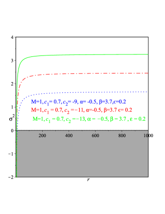
Figure 2: Schematic plot of solution (37) using Eqs. (39) and (40), namely, $\sigma^{2}$ versus the coordinate, $r$.

VI Thermodynamics of “p=2” and cubic black holes

In this section, we investigated the thermodynamics behavior of the BH solutions (15) and (37), from Eqs. (39) and (40), that are related to the quadratic and cubic forms of the field equations (8). To do this, we gave the basic definitions of the thermodynamical quantities.

VI.1 Thermodynamics of “p=2”

The metric potential of the temporal component of Eq. (15) takes the following form:

$$\mu(r)=1-\frac{2m}{r}+\epsilon\left[-\frac{c_{1}}{r}+c_{2}-\alpha\left(\frac{m^{2}+6mr+r^{2}}{mr^{3}}-\frac{16\left(1-\frac{2m}{r}\right)^{3/2}}{3m^{2}}+\frac{(1-\frac{3m}{r})}{2m^{2}}\ln\left(1-\frac{2m}{r}\right)\right)\right]$$

$$\simeq 1+\epsilon\Bigg{[}c_{2}+\frac{\alpha\{64-9ln(2)\}}{12m^{2}}\Bigg{]}-\frac{1}{r}\Bigg{[}2m+\epsilon\Bigg{(}c_{1}+\frac{16\alpha}{m}\Bigg{)}\Bigg{]}-O\Big{(}\frac{1}{r^{5}}\Big{)}\,.$$

Equation (VI.1) was draw in Fig. 32(a), the plot indicates the one horizon of the BH which can be obtained in a precise form from the solution of Eq. $\mu(r)=0$. This horizon is known as the event horizon $r_{h}$. One can calculate the total mass contained $r_{h}$. This can be done by setting $\mu(r_{h})=0$, and then we obtain the horizon mass-radius relation in the following form

$${m_{h}}=\frac{3r_{h}{}^{2}+\epsilon(3r_{h}{}^{2}c_{2}-32\alpha-3r_{h}c_{1})-9\epsilon\alpha ln(2)}{6r_{h}}\,.$$ (44)

Equation (44) is plotted in Fig. 32(b), whereas $m_{h}$ has positive and negative values, the BH has one horizon when $m_{h}=m_{min}$. This result is consistent with Fig. 32(a).

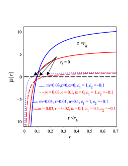
(a)  Possible one horizon

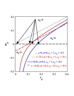
(b)  The horizon mass-radius

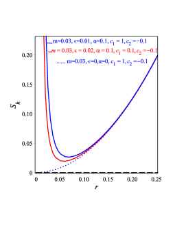
(c)  The horizon Bekenstein-Hawking entropy

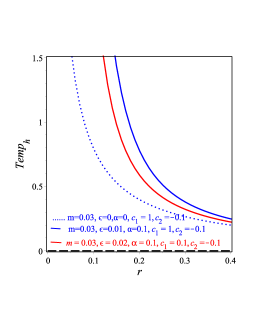
(d)  The horizon Hawking Temperature

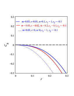
(e)  The horizon heat capacity

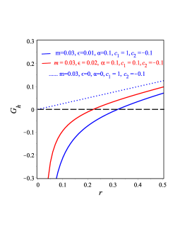
(f)  The horizon Gibbs free energy

Figure 3: Schematic plots of the thermodynamical quantities of the BH solution (15) for positive value of $\epsilon$: 2(a) Typical behavior of the metric function $\mu(r)$ given by (15); 2(b) the horizon mass–radius relation (44); 2(c) Typical behavior of the horizon entropy, which shows that $S_{h}$ increases quadratically as $r_{h}$ increases and we have always a positive entropy; 2(d) Typical behavior of the horizon temperature, (49), and 2(e) the heat capacity, (51), which show that both vanish at $r_{h}$, and we have always positive temperature and negative heat capacity which shows that the BH is unstable; 2(f) Typical behavior of the horizon Gibbs free energy which shows that $G_{h}$ have negative value as $r<r_{h}$ and positive value as $r>r_{h}$ for positive $\epsilon$.

The Hawking temperature is usually defined as Sheykhi (2012, 2010); Hendi et al. (2010); Sheykhi et al. (2010)

$$T_{h}=\frac{\mu^{\prime}(r_{h})}{4\pi},$$ (45)

where the event horizon $r=r_{h}$ is the positive solution of the equation $\mu(r_{h})=0$ which satisfies $\mu^{\prime}(r_{h})\neq 0$. In the framework of $f(T)$ gravity, the entropy is given by Cognola et al. (2011); Zheng and Yang (2018)

$$S(r_{h})=\frac{1}{4}Af_{T}(r_{h}),$$ (46)

where $A$ represents the area.

The constraint $\mu(r_{h})=0$ yields

$${r_{h}}_{{}_{{}_{{}_{{}_{``p=2"}}}}}\simeq\frac{12m^{2}+\epsilon[(6mc_{1}+32\alpha-12c_{2}m^{2})+9\alpha ln(2)]}{6m}\,.$$ (47)

When $\epsilon=0$ we get the GR limit.

From Eq. (46), the entropy of solution (15) takes the form

$${S_{h}}_{{}_{{}_{{}_{{}_{``p=2"}}}}}=\frac{\pi[r_{h}{}^{5}+2\epsilon\alpha m^{2}(4m+3r_{h})]}{r_{h}{}^{3}}\,,$$ (48)

which shows that when $\epsilon=0$ we get the GR entropy. Equation (48) shows that the parameters $\epsilon$ and $\alpha$ should be either positive or negative to get positive entropy otherwise the entropy will have a negative quantity. The behaviour of Eq. (48) is shown in Fig. 32(c) for positive values of $\epsilon$ and $\alpha$ which shows positive value of entropy.

The Hawking temperatures of solution (15) takes the form,

$${T_{h}}_{{}_{{}_{{}_{{}_{``p=2"}}}}}\simeq\frac{3r_{h}{}^{2}+\epsilon[\alpha(64-9ln(2))+3c_{2}r_{h}{}^{2}]}{12\pi r^{3}}\,.$$ (49)

Equation (49) shows that when $\epsilon=0$ we get the Hawking temperature of Schwarzschild BH. We depicted the Hawking’s temperature in Fig. 32(d) for positive values of $\epsilon$ and $\alpha$. Fig. 3 2(d) proves that we do have a positive temperature for the BH (15) and the temperature may take a negative value when either $\epsilon$ or $\alpha$ become a negative.

The stability of the BH solution is an important topic that can be studied on the dynamical and the perturbative levels Nashed (2003); Myung (2011, 2013). To investigate the thermodynamical stability of BH solution one derives the formula of the heat capacity $C(r_{h})$ at the event horizon. The event horizon heat capacity is given by the following from Nouicer (2007); Dymnikova and Korpusik (2011); Chamblin et al. (1999):

$$C_{h}\equiv C(r_{h})=\frac{\partial m_{h}}{\partial T}=\frac{\partial m_{h}}{\partial r_{h}}\left(\frac{\partial T}{\partial r_{h}}\right)^{-1}\,.$$ (50)

The BH will be thermodynamically stable, if its heat capacity $C_{h}$ is positive, and will be unstable if $C_{h}$ is negative. Using (44) and (49) into (50), we obtain the heat capacity as

$${C_{h}}_{{}_{{}_{{}_{{}_{``p=2``}}}}}=\frac{2\pi r_{h}^{2}}{3}\frac{3r_{h}{}^{2}+\epsilon[3r_{h}{}^{2}c_{2}+9\alpha ln(2)+32\alpha]}{\epsilon[9\alpha ln(2)-r_{h}{}^{2}c_{2}-64\alpha]-r_{h}{}^{2}}\,.$$ (51)

Equation (51) shows that $C_{h}$ does not locally diverge and the BH has no phase transition of second-order. The heat capacity is depicted in Fig. 32(e) which shows that $C_{h}<0$ where $r_{h}<r_{dg}$ and the BH is thermodynamically unstable. The main reason that makes the heat capacity negative is the derivative of Hawking temperature and this is consistent with the nature of Schwarzschild black hole which can be discovered when $\epsilon=0$. In the non-vanishing of $\epsilon$ we can create a positive heat capacity but the price of this is to accept the Hawking temperature to has a negative value.

The Gibbs free energy is given by Zheng and Yang (2018); Kim and Kim (2012)

$$G(r_{h})=m(r_{h})-T(r_{h})S(r_{h})\,.$$ (52)

The quantities $m(r_{h})$, $T(r_{h})$ and $S(r_{h})$ are the mass, temperature and entropy at the event horizon, respectively. From Eqs. (44), (48) and (49) in (52), we obtain

$${G_{h}}_{{}_{{}_{{}_{{}_{\tiny Eq.(\ref{bfin})}}}}}=\frac{3r_{h}{}^{5}+\epsilon[3r_{h}{}^{5}c_{2}-9\alpha r_{h}{}^{3}ln(2)-128\alpha r_{h}{}^{3}-6r_{h}{}^{4}c_{1}-6m^{2}\{3\alpha r_{h}+4\alpha m^{2}\}]}{12r_{h}{}^{4}}.$$ (53)

We depict the Gibbs energy of the black hole (15) in Fig. 32(f), which indicates that the Gibbs energy has negative values at large $r<r_{h}$ and positive value when $r>r_{h}$. We note that for $\epsilon=0$, the Schwarzschild black hole is recovered which is shown in Fig. 32(f) by the blue dot curve. Interestingly, for the negative value of $\epsilon$, Gibbs energy is always positive, and as we discuss before that the price of this is the negative Hawking temperature. We depict the case of a negative value of $\epsilon$ in Fig. 4.

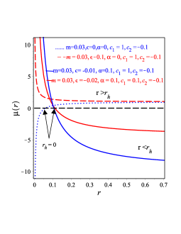
(a)  Possible one horizon

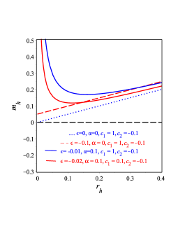
(b)  The horizon mass-radius

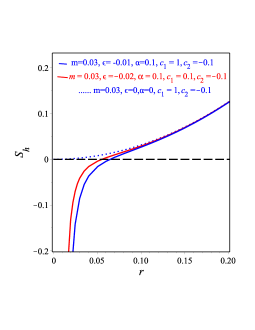
(c)  The horizon Bekenstein-Hawking entropy

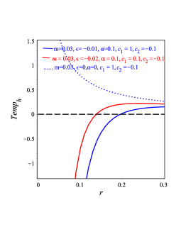
(d)  The horizon Hawking Temperature

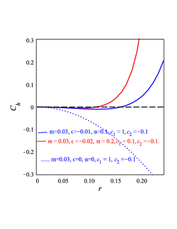
(e)  The horizon heat capacity

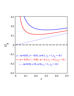
(f)  The horizon Gibbs free energy

Figure 4: Schematic plots of thermodynamical quantities of the BH solution (15) for negative value of $\epsilon$: 3(a) Typical behavior of the metric function $\mu(r)$ given by (15); 3(b) the horizon mass–radius relation (44); 3(c) typical behavior of the horizon entropy, which shows that $S_{h}$ increases quadratically as $r_{h}$ increases and as $r<r_{h}$ we have a negative entropy and as $r>r_{h}$ we have a positive entropy; 3(d) typical behavior of the horizon temperature, and 3(e) the heat capacity, (51), which shows that both vanish at $r_{h}$, and as $r<r_{h}$ we have a negative temperature and heat capacity and as $r>r_{h}$ we have a positive values of both the BH is unstable (i.e $C_{h}<0$) when $r<r_{h}$ and it is stable (i.e $C_{h}>0$) when $r>r_{h}$; 3(f) typical behavior of the horizon Gibbs free energy which shows that $G_{h}$ could have only positive values for negative value of $\epsilon$.

VI.2 Thermodynamics of the cubic solution

The metric potential of the temporal component of solution (37), using Eqs. (39) and (40) takes the form

$$\mu(r)\simeq 1+\epsilon\Bigg{[}\frac{1260m^{4}c_{2}-\alpha m^{2}\{945ln(2)ln(2)-6720\}-\beta\{4410ln(2)+8192\}}{1260m^{4}}\Bigg{]}$$

$$-\frac{1}{135m^{3}r}\Bigg{[}270m^{4}+\epsilon\Bigg{(}135m^{3}c_{1}+2160\alpha m^{2}+2048\beta\Bigg{)}\Bigg{]}-O\Big{(}\frac{1}{r^{5}}\Big{)}\,.$$

Equation (VI.2) is drawn in Fig. 52(a), the plot shows that the BH could have one horizon at the root of $\mu(r)=0$, this is the event horizon $r_{h}$. The horizon mass-radius relation of solution (37), using Eqs. (39) and (40) has the form

$${m_{h}}=\frac{135r_{h}{}^{4}+\epsilon[135r_{h}{}^{4}c_{2}-405\alpha r_{h}{}^{2}-135r_{h}{}^{3}c_{1}-405n\alpha ln(2)r_{h}{}^{2}-16348\beta]}{720r_{h}{}^{3}}\,.$$ (55)

We plot the above relation in Fig. 54(b), whereas $m_{h}$ has positive and negative values, the black hole has one horizon when $m_{h}=m_{min}$. This result is in agreement with Fig. 54(a).

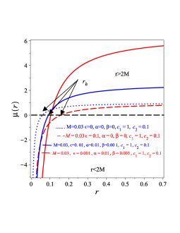
(a)  Possible one horizon

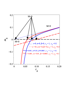
(b)  The horizon mass-radius

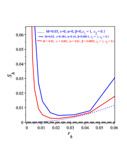
(c)  The horizon Bekenstein-Hawking entropy

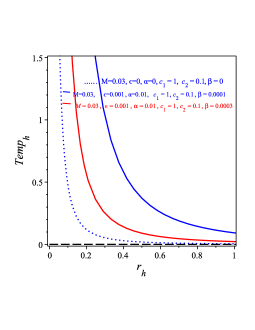
(d)  The horizon Hawking Temperature

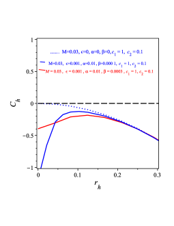
(e)  The horizon heat capacity

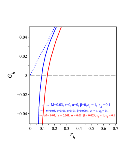
(f)  The horizon Gibbs free energy

Figure 5: Schematic plots of thermodynamical quantities of the BH solution (37), using Eqs. (39) and (40) for positive value of $\epsilon$: 4(a) Typical behavior of the metric function $\mu(r)$ given by (VI.2); 4(b) the horizon mass–radius relation (44); 4(c) typical behavior of the horizon entropy, which shows that $S_{h}$ increases quadratically as $r_{h}$ increases and we have always a positive entropy; 4(d) typical behavior of the horizon temperature, and 4(e) the heat capacity, (51), which show that both vanish at $r_{h}$, and we have always positive temperature and negative heat capacity; 4(f) typical behavior of the horizon Gibbs free energy which shows that $G_{h}$ could have negative value at $r<r_{h}$ and positive value at $r>r_{h}$ for negative value of $\epsilon$.

The constraint $\mu(r_{h})=0$ yields

$${r_{h}}_{{}_{{}_{{}_{{}_{cubic}}}}}\simeq\frac{3780m^{4}+\epsilon[4096\beta+10080\alpha m^{2}+1890c_{1}m^{3}+13230\beta ln(2)+2835\alpha m^{2}ln(2)-3780c_{2}m^{4}]}{1890m^{3}}\,.$$ (56)

When $\epsilon=0$ Eq. (56) gives the GR limit.

From Eq. (46), the entropy of solution (37) takes the form

$${S_{h}}_{{}_{{}_{{}_{{}_{cubic}}}}}=\frac{\pi}{r_{h}{}^{2}(r_{h}{}^{2}-4m^{2})^{2}}\Bigg{[}r_{h}{}^{4}(r_{h}{}^{2}-4m^{2})^{2}+4\epsilon\Big{\{}r_{h}{}^{6}\alpha+16\beta m^{4}+8\alpha r_{h}{}^{2}m^{4}-6\alpha r_{h}{}^{4}m^{2}+8\beta m^{3}r_{h}$$

$$+\Big{\{}8[\beta m-\alpha r_{h}]r_{h}{}^{2}-m[16\beta m^{2}-\alpha r_{h}{}^{4}]+4r_{h}m^{2}[4\beta-mr_{h}\alpha]+r_{h}{}^{3}\alpha[4m^{2}-r_{h}{}^{2}]\Big{\}}\sqrt{r_{h}{}^{2}+2mr_{h}}$$

$$+4\beta r_{h}{}^{2}[2r_{h}{}^{2}-7m^{2}]\Bigg{]}\,,$$ (57)

which shows that when $\epsilon=0$ we recover the entropy of GR. Equation (VI.2) shows that the parameters $\epsilon$, $\alpha$ and $\beta$ should be either positive or negative to get positive entropy otherwise the entropy will have a negative quantity. The behavior of Eq. (VI.2) is shown in Fig. 54(c) for positive values of $\epsilon$ and $\alpha$ which shows positive value of entropy.

The Hawking temperatures of solution (37) takes the form,

$${T_{h}}_{{}_{{}_{{}_{{}_{cubic}}}}}\simeq\frac{3r_{h}{}^{2}+\epsilon[\alpha(64-9ln(2))+3c_{2}r_{h}{}^{2}]}{12\pi r_{h}{}^{3}}\,,$$ (58)

which is identical with the quadratic form up to $\epsilon$ but with different value of $\alpha$ to unify the values through all the calculations of cubic case. Therefore, same discussions carried out for the case of quadratic can be applied here.

Using (55) and (58) into (50), we obtain the heat capacity as

$${C_{h}}_{{}_{{}_{{}_{{}_{cubic}}}}}=\frac{2\pi}{45}\frac{45r_{h}{}^{4}+\epsilon[45r_{h}{}^{4}c_{2}+135r_{h}{}^{2}\alpha ln(2)+480r_{h}{}^{2}\alpha+16348\beta]}{\epsilon[9\alpha ln(2)-r_{h}{}^{2}c_{2}-64\alpha]-r_{h}{}^{2}}\,.$$ (59)

Equation (59) shows that $C_{h}$ does not locally diverge and the black hole has no phase transition of second-order. The heat capacity is depicted in Fig. 54(e) which shows that $C_{h}<0$ where $r_{h}<r_{dg}$ and the black hole is thermodynamically unstable. The main reason that makes the heat capacity negative is the derivative of Hawking temperature and this is consistent with the Schwarzschild black hole which can be discovered when $\epsilon=0$. In the non-vanishing of $\epsilon$ we can create a positive heat capacity but the price of this is to accept the Hawking temperature to has a negative value.

From Eqs. (55), (VI.2) and (58) in (52), we obtain

$${G_{h}}_{{}_{{}_{{}_{{}_{cubic}}}}}=\frac{\pi}{540r_{h}{}^{3}(r_{h}{}^{2}-4m^{2})^{2}}\Bigg{[}135r_{h}{}^{4}(r_{h}{}^{2}-4m^{2})^{2}-\epsilon\Bigg{\{}4(1575r_{h}{}^{6}\alpha+9272r_{h}{}^{4}\beta+133232\beta m^{4})-135r_{h}{}^{7}[r_{h}c_{2}-2c_{1}]$$

$$-16r_{h}m^{2}\beta[17329r_{h}-270m]+1080c_{2}m^{2}r_{h}{}^{4}[r_{h}{}^{2}-2m^{2}]-2160m^{2}r_{h}{}^{3}c_{1}[r_{h}{}^{2}-2m^{2}]+405r_{h}{}^{6}\alpha ln(2)$$

$$+\Big{\{}2160r_{h}m^{2}[4\beta+\alpha r_{h}{}^{2}]+540r_{h}{}^{2}\alpha m[r_{h}{}^{2}-4m^{2}]-4320\beta m[2m^{2}-4r_{h}{}^{2}]-540r_{h}{}^{3}[8\beta+r_{h}{}^{2}\alpha]\Big{\}}\sqrt{r_{h}{}^{2}+2mr_{h}}$$

$$-10r_{h}{}^{2}m^{2}\alpha[4932r_{h}{}^{2}-9648m^{2}-648m^{2}ln(2)+324r_{h}{}^{2}ln(2)]\Bigg{\}}\Bigg{]}.$$ (60)

We depict Gibbs energy of the black hole (37) in Fig. 54(f), which indicates that the Gibbs energy has negative values at large $r<r_{h}$ and positive value when $r>r_{h}$. We note that for $\epsilon=0$, the Scharzschild black hole is recovered which is shown in Fig. 54(f) by the blue dot curve. Interestingly, for negative value of $\epsilon$, Gibbs energy is always positive and as we discuss before that the price of this is the negative Hawking temperature. We depict the case of negative value of $\epsilon$ in Fig. 6.

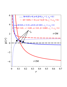
(a)  Possible one horizon

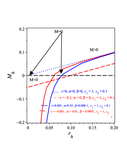
(b)  The horizon mass-radius

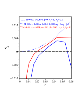
(c)  The horizon Bekenstein-Hawking entropy

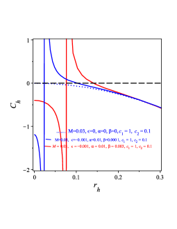
(d)  The horizon heat capacity

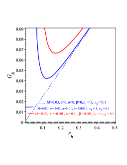
(e)  The horizon Gibbs free energy

Figure 6: Schematic plots of thermodynamical quantities of the black hole solution (37) for negative value of $\epsilon$: 5(a) Typical behavior of the metric function $\mu(r)$ given by (37); 5(b) the horizon mass–radius relation (44); 5(c) typical behavior of the horizon entropy, which shows that $S_{h}$ increases quadratically as $r_{h}$ increases and then decrease; 5(d) typical behavior of the heat capacity, (59), which shows that it vanish at $r_{h}$, and as $r<r_{h}$ we have a positive heat capacity and as $r>r_{h}$ we have a negative value of the black hole; 5(e) typical behavior of the horizon Gibbs free energy which shows that $G_{h}$ have always positive value for negative value of $\epsilon$.

We summarize the results of thermodynamics of the quadratic and cubic cases in table I. As this table shows that when the parameter $\epsilon$ takes positive value we have good models.

Table 1: The main results thermodynamic according to the values of $\epsilon$, i.e., positive or negative values.

			Quadratic
$\epsilon$	Entropy	Temperature		Heat capacity	Gibb’s free energy
zero	positive	positive		negative	positive
$>$zero	positive	positive		negative	positive(conditional)
$<$zero	positive(conditional)	positive(conditional)		positive(conditional)	positive
			Cubic
zero	positive	positive		negative	positive
$>$zero	positive	positive		negative	positive(conditional)
$<$zero	positive(conditional)	positive(conditional)		positive(conditional)	positive

VII Discussion and conclusions

In this study, we further studied $f(T)$ in the framework of the spherically symmetric space-time. To do this, we used a physical tetrad field space-time possessing two unknown functions. This study aims to determine the physics of the BH that was derived in Bahamonde et al. (2019) for the quadratic form of $f(T)$. We calculated the invariants of this BH and demonstrated that the behavior of the tensors $T^{\alpha\beta\gamma}T_{\alpha\beta\gamma}=T^{\alpha}T_{\alpha}=T\sim{r^{-2}}$ are similar to the results obtained before in the frame of $f(T)$ Nashed and Saridakis (2019); Awad et al. (2017), and dissimilar to the solutions of GR and TEGR, which behaved as $T^{\alpha\beta\gamma}T_{\alpha\beta\gamma}=T^{\alpha}T_{\alpha}=T\sim{r^{-4}}$. This clearly indicated that the contribution of the higher-order torsion made the singularity of $T^{\alpha\beta\gamma}T_{\alpha\beta\gamma}$, $T^{\alpha}T_{\alpha}$ and $T$ milder. Additionally, we calculated the energy content and revealed the contribution of the higher-order torsion. Finally, we calculated the stability of this BH via the geodesic deviation and revealed the regions where the BH exhibited stability, as shown in Fig. 1.

In the second part, we presented the cubic form of the field equations using $f(T)=T+\epsilon\Big{[}\frac{1}{2}\alpha T^{2}+\frac{1}{3}\beta T^{3}\Big{]}$ and derived the asymptotic form of these field equations up to $O(\epsilon)$. The derived BH solution was characterized by the mass, the two constants of integrations and the three constants that characterized the form $f(T)$. The asymptotic form of this BH behaved like a flat space-time. We calculated the invariants of this BH and its energy thereby revealed the contribution of the higher-order torsion to the energy. Furthermore, we calculated the geodesic deviation and revealed where the regions of stability in the BH. To study the BH solutions of this study in-depth we calculated the thermodynamic quantities including the Hawking temperature, entropy, heat capacity, and Gibbs energy for the quadratic and cubic forms of the BH solutions. For the quadratic form, we used the same values of the constants that are used for the stability study. We studied all the thermodynamical quantities with two values of the parameters $\epsilon$ the positive value and negative values as shown in figures 3 and 4. The most beneficial results that were discussed were those of the entropy, Hawking temperature, heat capacity, and Gibbs energy. At $\epsilon>0$ positive values were always obtained for the entropy and temperature while a negative value was obtained for the heat capacity. Regarding the Gibbs energy, we obtained a negative value at $r_{dg}<r_{h}$ and a positive one at $r_{dg}>r_{h}$. At $\epsilon<0$ those quantities were negative regarding the entropy at $r_{dg}<r_{h}$ and positive at $r_{dg}>r_{h}$. Furthermore, regarding the temperature and heat capacity the values were negative at $r_{dg}<r_{h}$ and positive at $r_{dg}>r_{h}$. Regarding the Gibbs energy it was always positive and we concluded that $\epsilon$ of the quadratic form might be positive or negative values and both of them afforded the physical thermodynamic quantities. The same discussion is applicable for the cubic BH.

References

- Bahamonde et al. (2019) Sebastian Bahamonde, Kai Flathmann, and Christian Pfeifer, “Photon sphere and perihelion shift in weak gravity,” (2019), arXiv:1907.10858 [gr-qc] .
- Capozziello and De Laurentis (2011) Salvatore Capozziello and Mariafelicia De Laurentis, “Extended theories of gravity,” Physics Reports 509, 167–321 (2011).
- Clifton et al. (2012) Timothy Clifton, Pedro G. Ferreira, Antonio Padilla, and Constantinos Skordis, “Modified gravity and cosmology,” Physics Reports 513, 1–189 (2012).
- Heisenberg (2019) Lavinia Heisenberg, “A systematic approach to generalisations of general relativity and their cosmological implications,” Physics Reports 796, 1–113 (2019).
- Stetsko (2020) M. M. Stetsko, “Static spherically symmetric einstein-yang-mills-dilaton black hole and its thermodynamics,” (2020), arXiv:2005.13447 [hep-th] .
- Will (2014) Clifford M. Will, “The confrontation between general relativity and experiment,” Living Reviews in Relativity 17 (2014), 10.12942/lrr-2014-4.
- Carlip (2020) S. Carlip, “Near-horizon Bondi-Metzner-Sachs symmetry, dimensional reduction, and black hole entropy,” Phys. Rev. D 101, 046002 (2020), arXiv:1910.01762 [hep-th] .
- Unzicker and Case (2005) A. Unzicker and T. Case, “Translation of Einstein’s Attempt of a Unified Field Theory with Teleparallelism,” ArXiv Physics e-prints (2005), physics/0503046 .
- de Andrade et al. (2000) V. C. de Andrade, L. C. T. Guillen, and J. G. Pereira, “Teleparallel gravity: An overview,” (2000), arXiv:gr-qc/0011087 [gr-qc] .
- Nashed (2018) Gamal Nashed, “Charged and Non-Charged Black Hole Solutions in Mimetic Gravitational Theory,” Symmetry 10, 559 (2018).
- Aldrovandi et al. (2003) R. Aldrovandi, J. G. Pereira, and K. H. Vu, “Selected topics in teleparallel gravity,” (2003), arXiv:gr-qc/0312008 [gr-qc] .
- Maluf (2013) José W. Maluf, “The teleparallel equivalent of general relativity,” Annalen der Physik 525, 339–357 (2013).
- Shirafuji et al. (1996) T. Shirafuji, G. G. L. Nashed, and K. Hayashi, “Energy of general spherically symmetric solution in the tetrad theory of gravitation,” Progress of Theoretical Physics 95, 665–678 (1996).
- de Andrade and Pereira (1997) V. C. de Andrade and J. G. Pereira, “Gravitational lorentz force and the description of the gravitational interaction,” Physical Review D 56, 4689–4695 (1997).
- El Hanafy and Nashed (2016) W. El Hanafy and G. G. L. Nashed, “Exact teleparallel gravity of binary black holes,” Astrophysics and Space Science 361 (2016), 10.1007/s10509-016-2662-y.
- Nashed and Capozziello (2019a) Gamal G. L. Nashed and Salvatore Capozziello, “Magnetic black holes in weitzenböck geometry,” General Relativity and Gravitation 51 (2019a), 10.1007/s10714-019-2535-0.
- Nashed (2006a) G.G.L. Nashed, “Charged axially symmetric solution and energy in teleparallel theory equivalent to general relativity,” The European Physical Journal C 49, 851–857 (2006a).
- Nashed (2010) Gamal G. L. Nashed, “Brane World black holes in Teleparallel Theory Equivalent to General Relativity and their Killing vectors, Energy, Momentum and Angular-Momentum,” Chin. Phys. , 020401 (2010), arXiv:0910.5124 [gr-qc] .
- Nashed (2006b) G.G.L. Nashed, “Reissner-nordström solutions and energy in teleparallel theory,” Modern Physics Letters A 21, 2241–2250 (2006b), cited By 24.
- NASHED and SHIRAFUJI (2007) GAMAL G. L. NASHED and TAKESHI SHIRAFUJI, “Reissner–nordstrÖm space–time in the tetrad theory of gravitation,” International Journal of Modern Physics D 16, 65–79 (2007).
- ULHOA et al. (2010) S. C. ULHOA, J. F. DA ROCHA NETO, and J. W. MALUF, “The gravitational energy problem for cosmological models in teleparallel gravity,” International Journal of Modern Physics D 19, 1925–1935 (2010).
- Capozziello et al. (2011) S. Capozziello, V. F. Cardone, H. Farajollahi, and A. Ravanpak, “Cosmography inf(t)gravity,” Physical Review D 84 (2011), 10.1103/physrevd.84.043527.
- Nojiri and Odintsov (2011) Shin’ichi Nojiri and Sergei D. Odintsov, “Unified cosmic history in modified gravity: From theory to lorentz non-invariant models,” Physics Reports 505, 59–144 (2011).
- NOJIRI and ODINTSOV (2007) SHIN’ICHI NOJIRI and SERGEI D. ODINTSOV, “Introduction to modified gravity and gravitational alternative for dark energy,” International Journal of Geometric Methods in Modern Physics 04, 115–145 (2007).
- Nojiri et al. (2017) S. Nojiri, S.D. Odintsov, and V.K. Oikonomou, “Modified gravity theories on a nutshell: Inflation, bounce and late-time evolution,” Physics Reports 692, 1–104 (2017).
- Nashed and Capozziello (2019b) Gamal G. L. Nashed and Salvatore Capozziello, “Charged spherically symmetric black holes in gravity and their stability analysis,” Phys. Rev. D99, 104018 (2019b), arXiv:1902.06783 [gr-qc] .
- Bengochea (2011) Gabriel R. Bengochea, “Observational information for f(T) theories and Dark Torsion,” Phys. Lett. B 695, 405–411 (2011), arXiv:1008.3188 [astro-ph.CO] .
- Karami and Abdolmaleki (2013) Kayoomars Karami and Asrin Abdolmaleki, “f(t) modified teleparallel gravity as an alternative for holographic and new agegraphic dark energy models,” Research in Astronomy and Astrophysics 13, 757–771 (2013).
- Dent et al. (2011) James B Dent, Sourish Dutta, and Emmanuel N Saridakis, “f(t) gravity mimicking dynamical dark energy. background and perturbation analysis,” Journal of Cosmology and Astroparticle Physics 2011, 009–009 (2011).
- Cai et al. (2011) Yi-Fu Cai, Shih-Hung Chen, James B Dent, Sourish Dutta, and Emmanuel N Saridakis, “Matter bounce cosmology with the f ( t) gravity,” Classical and Quantum Gravity 28, 215011 (2011).
- Mai and Lü (2017) Zhan-Feng Mai and H. Lü, “Black holes, dark wormholes, and solitons in f(t) gravities,” Physical Review D 95 (2017), 10.1103/physrevd.95.124024.
- Ferraro and Fiorini (2008) Rafael Ferraro and Franco Fiorini, “Born-infeld gravity in weitzenböck spacetime,” Physical Review D 78 (2008), 10.1103/physrevd.78.124019.
- FIORINI and FERRARO (2009) FRANCO FIORINI and RAFAEL FERRARO, “A type of born-infeld regular gravity and its cosmological consequences,” International Journal of Modern Physics A 24, 1686–1689 (2009).
- Cardone et al. (2012) Vincenzo F. Cardone, Ninfa Radicella, and Stefano Camera, “Acceleratingf(t)gravity models constrained by recent cosmological data,” Physical Review D 85 (2012), 10.1103/physrevd.85.124007.
- Myrzakulov (2011) Ratbay Myrzakulov, “Accelerating universe from f(t) gravity,” The European Physical Journal C 71 (2011), 10.1140/epjc/s10052-011-1752-9.
- Yang (2011) Rong-Jia Yang, “New types of f(t) gravity,” The European Physical Journal C 71 (2011), 10.1140/epjc/s10052-011-1797-9.
- Bamba et al. (2013) Kazuharu Bamba, Sergei D. Odintsov, and Diego Sáez-Gómez, “Conformal symmetry and accelerating cosmology in teleparallel gravity,” Physical Review D 88 (2013), 10.1103/physrevd.88.084042.
- Camera et al. (2014) Stefano Camera, Vincenzo F. Cardone, and Ninfa Radicella, “Detectability of torsion gravity via galaxy clustering and cosmic shear measurements,” Physical Review D 89 (2014), 10.1103/physrevd.89.083520.
- Nashed (2015) G. L. Nashed, “Frw in quadratic form of f(t) gravitational theories,” General Relativity and Gravitation 47 (2015), 10.1007/s10714-015-1917-1.
- Nashed (2013a) Gamal G. L. Nashed, “Spherically symmetric charged-dS solution in gravity theories,” Phys. Rev. D88, 104034 (2013a), arXiv:1311.3131 [gr-qc] .
- Wang (2011) Tower Wang, “Static solutions with spherical symmetry inf(t)theories,” Physical Review D 84 (2011), 10.1103/physrevd.84.024042.
- Rodrigues et al. (2013) M. E. Rodrigues, M. J. S. Houndjo, J. Tossa, D. Momeni, and R. Myrzakulov, “Charged Black Holes in Generalized Teleparallel Gravity,” JCAP 11, 024 (2013), arXiv:1306.2280 [gr-qc] .
- Ferraro and Fiorini (2011) Rafael Ferraro and Franco Fiorini, “Spherically symmetric static spacetimes in vacuum f(T) gravity,” Phys. Rev. D 84, 083518 (2011), arXiv:1109.4209 [gr-qc] .
- Nashed (2013b) Gamal G. L. Nashed, “A special exact spherically symmetric solution in f(T) gravity theories,” Gen. Rel. Grav. 45, 1887–1899 (2013b), arXiv:1502.05219 [gr-qc] .
- Junior et al. (2015) Ednaldo L. B. Junior, Manuel E. Rodrigues, and Mahouton J. S. Houndjo, “Regular black holes in Gravity through a nonlinear electrodynamics source,” JCAP 1510, 060 (2015), arXiv:1503.07857 [gr-qc] .
- Iorio and Saridakis (2012) Lorenzo Iorio and Emmanuel N. Saridakis, “Solar system constraints on f(T) gravity,” Mon. Not. Roy. Astron. Soc. 427, 1555 (2012), arXiv:1203.5781 [gr-qc] .
- Xie and Deng (2013) Yi Xie and Xue-Mei Deng, “ gravity: effects on astronomical observation and Solar System experiments and upper-bounds,” Mon. Not. Roy. Astron. Soc. 433, 3584–3589 (2013), arXiv:1312.4103 [gr-qc] .
- Ruggiero and Radicella (2015) Matteo Luca Ruggiero and Ninfa Radicella, “Weak-Field Spherically Symmetric Solutions in gravity,” Phys. Rev. D 91, 104014 (2015), arXiv:1501.02198 [gr-qc] .
- Awad et al. (2018) A. Awad, W. El Hanafy, G. G. L. Nashed, and Emmanuel N. Saridakis, “Phase Portraits of general f(T) Cosmology,” JCAP 1802, 052 (2018), arXiv:1710.10194 [gr-qc] .
- Awad et al. (2017) A. M. Awad, S. Capozziello, and G. G. L. Nashed, “-dimensional charged Anti-de-Sitter black holes in gravity,” JHEP 07, 136 (2017), arXiv:1706.01773 [gr-qc] .
- Chen et al. (2020) Zhaoting Chen, Wentao Luo, Yi-Fu Cai, and Emmanuel N. Saridakis, “New test on general relativity and torsional gravity from galaxy-galaxy weak lensing surveys,” Phys. Rev. D 102, 104044 (2020), arXiv:1907.12225 [astro-ph.CO] .
- Cai et al. (2016) Yi-Fu Cai, Salvatore Capozziello, Mariafelicia De Laurentis, and Emmanuel N. Saridakis, “f(T) teleparallel gravity and cosmology,” Rept. Prog. Phys. 79, 106901 (2016), arXiv:1511.07586 [gr-qc] .
- Weitzenböck (1923) R. Weitzenböck, Invariance Theorie (Gronin-gen, 1923).
- Clarke and Królak (1985) C.J.S. Clarke and A. Królak, “Conditions for the occurence of strong curvature singularities,” Journal of Geometry and Physics 2, 127 – 143 (1985).
- Tipler (1977) Frank J. Tipler, “Singularities in conformally flat spacetimes,” Physics Letters A 64, 8 – 10 (1977).
- ULHOA and SPANIOL (2013) S. C. ULHOA and E. P. SPANIOL, “On the gravitational energy–momentum vector in f(t) theories,” International Journal of Modern Physics D 22, 1350069 (2013).
- Maluf et al. (2006) J W Maluf, S C Ulhoa, F F Faria, and J F da Rocha-Neto, “The angular momentum of the gravitational field and the poincaré group,” Classical and Quantum Gravity 23, 6245–6256 (2006).
- Misner et al. (1973) Charles W. Misner, K.S. Thorne, and J.A. Wheeler, Gravitation (W. H. Freeman, San Francisco, 1973).
- D’Inverno (1992) R. A. D’Inverno, Internationale Elektronische Rundschau (1992).
- Nashed (2003) Gamal G. L. Nashed, “Stability of the vacuum nonsingular black hole,” Chaos Solitons Fractals 15, 841 (2003), arXiv:gr-qc/0301008 [gr-qc] .
- Nashed and Saridakis (2019) G. G. L. Nashed and Emmanuel N. Saridakis, “Rotating AdS black holes in Maxwell- gravity,” Class. Quant. Grav. 36, 135005 (2019), arXiv:1811.03658 [gr-qc] .
- Sheykhi (2012) Ahmad Sheykhi, “Higher-dimensional charged black holes,” Phys. Rev. D 86, 024013 (2012).
- Sheykhi (2010) Ahmad Sheykhi, “Thermodynamics of apparent horizon and modified Friedmann equations,” Eur. Phys. J. C69, 265–269 (2010), arXiv:1012.0383 [hep-th] .
- Hendi et al. (2010) S. H. Hendi, A. Sheykhi, and M. H. Dehghani, “Thermodynamics of higher dimensional topological charged AdS black branes in dilaton gravity,” Eur. Phys. J. C70, 703–712 (2010), arXiv:1002.0202 [hep-th] .
- Sheykhi et al. (2010) A. Sheykhi, M. H. Dehghani, and S. H. Hendi, “Thermodynamic instability of charged dilaton black holes in ads spaces,” Phys. Rev. D 81, 084040 (2010).
- Cognola et al. (2011) G. Cognola, O. Gorbunova, L. Sebastiani, and S. Zerbini, “Energy issue for a class of modified higher order gravity black hole solutions,” Phys. Rev. D 84, 023515 (2011).
- Zheng and Yang (2018) Yaoguang Zheng and Rong-Jia Yang, “Horizon thermodynamics in theory,” Eur. Phys. J. C78, 682 (2018), arXiv:1806.09858 [gr-qc] .
- Myung (2011) Yun Soo Myung, “Instability of a rotating black hole in a limited form off(r)gravity,” Physical Review D 84 (2011), 10.1103/physrevd.84.024048.
- Myung (2013) Yun Soo Myung, “Instability of a Kerr black hole in gravity,” Phys. Rev. D 88, 104017 (2013), arXiv:1309.3346 [gr-qc] .
- Nouicer (2007) Khireddine Nouicer, “Black holes thermodynamics to all order in the Planck length in extra dimensions,” Class. Quant. Grav. 24, 5917–5934 (2007), [Erratum: Class. Quant. Grav.24,6435(2007)], arXiv:0706.2749 [gr-qc] .
- Dymnikova and Korpusik (2011) Irina Dymnikova and Michał Korpusik, “Thermodynamics of regular cosmological black holes with the de sitter interior,” Entropy 13, 1967–1991 (2011).
- Chamblin et al. (1999) Andrew Chamblin, Roberto Emparan, Clifford V. Johnson, and Robert C. Myers, “Charged AdS black holes and catastrophic holography,” Phys. Rev. D60, 064018 (1999), arXiv:hep-th/9902170 [hep-th] .
- Kim and Kim (2012) Wontae Kim and Yongwan Kim, “Phase transition of quantum corrected Schwarzschild black hole,” Phys. Lett. B718, 687–691 (2012), arXiv:1207.5318 [gr-qc] .
- Awad et al. (2017) A. M. Awad, S. Capozziello, and G. G. L. Nashed, “D-dimensional charged Anti-de-Sitter black holes in f ( T) gravity,” Journal of High Energy Physics 7, 136 (2017), arXiv:1706.01773 [gr-qc] .