Breaking $O(nr)$ for Matroid Intersection

Abstract

We present algorithms that break the $\tilde{O}(nr)$-independence-query bound for the Matroid Intersection problem for the full range of $r$; where $n$ is the size of the ground set and $r\leq n$ is the size of the largest common independent set. The $\tilde{O}(nr)$ bound was due to the efficient implementations [CLSSW FOCS’19; Nguyễn 2019] of the classic algorithm of Cunningham [SICOMP’86]. It was recently broken for large $r$ ($r=\omega(\sqrt{n})$), first by the ${\tilde{O}}(n^{1.5}/\varepsilon^{1.5})$-query $(1-\varepsilon)$-approximation algorithm of CLSSW [FOCS’19], and subsequently by the ${\tilde{O}}(n^{6/5}r^{3/5})$-query exact algorithm of BvdBMN [STOC’21]. No algorithm—even an approximation one—was known to break the $\tilde{O}(nr)$ bound for the full range of $r$. We present an ${\tilde{O}}(n\sqrt{r}/\varepsilon)$-query $(1-\varepsilon)$-approximation algorithm and an ${\tilde{O}}(nr^{3/4})$-query exact algorithm. Our algorithms improve the $\tilde{O}(nr)$ bound and also the bounds by CLSSW and BvdBMN for the full range of $r$.

1 Introduction

Matroid Intersection is a fundamental problem in combinatorial optimization that has been studied for more than half a century. The classic version of this problem is as follows: Given two matroids ${\mathcal{M}}_{1}=(V,{\mathcal{I}}_{1})$ and ${\mathcal{M}}_{2}=(V,{\mathcal{I}}_{2})$ over a common ground set $V$ of $n$ elements, find the largest common independent set $S^{*}\in{\mathcal{I}}_{1}\cap{\mathcal{I}}_{2}$ by making independence oracle queries of the form “Is $S\in{\mathcal{I}}_{1}$?” or “Is $S\in{\mathcal{I}}_{2}$?” for $S\subseteq V$. The size of the largest common independent set is usually denoted by $r$.

Matroid intersection can be used to model many other combinatorial optimization problems, such as bipartite matching, arborescences, spanning tree packing, etc. As such, designing algorithms for matroid intersection is an interesting problem to study.

In this paper, we consider the task of finding a $(1-\varepsilon)$-approximate solution to the matroid intersection problem, that is finding some common independent set $S$ of size at least $(1-\varepsilon)r$. We show an improvement of approximation algorithms for matroid intersection, and as a consequence also obtain an improvement for the exact matroid intersection problem.

Previous work.

Polynomial algorithms for matroid intersection started with the work of Edmond’s $O(n^{2}r)$-query algorithms [EDVJ68, Edm70, Edm79] in the 1960s. Since then, there has been a long line of research e.g. [AD71, Law75, Cun86, LSW15, CQ16, CLS⁺19, BvdBMN21]. Cunningham [Cun86] designed a $O(nr^{1.5})$-query blocking-flow algorithm in 1986, similar to that of Hopcroft-Karp’s bipartite-matching or Dinic’s maximum-flow algorithms. Chekuri and Quanrud [CQ16] pointed out that Cunningham’s classic algorithm [Cun86] from 1986 is already a $O(nr/\varepsilon)$-query $(1-\epsilon)$-approximation algorithm. Recently, Chakrabarty-Lee-Sidford-Singla-Wong [CLS⁺19] and Nguyễn [Ngu19] independently showed how to implement Cunningham’s classic algorithm using only ${\tilde{O}}(nr)$ independence queries. This is akin to spending $\tilde{O}(n)$ queries to find each of the so-called augmenting paths. A fundamental question is whether several augmenting paths can be found simultaneously to break the $\tilde{O}(nr)$ bound.

This question has been answered for large $r$ ($r=\omega(\sqrt{n})$), first by the ${\tilde{O}}(n^{1.5}/\varepsilon^{1.5})$-query $(1-\epsilon)$-approximation algorithm of Chakrabarty-Lee-Sidford-Singla-Wong [CLS⁺19], and very recently by the randomized ${\tilde{O}}(n^{6/5}r^{3/5})$-query exact algorithm of Blikstad-v.d.Brand-Mukhopadhyay-Nanongkai [BvdBMN21]. Whether we can break the $O(nr)$-query bound for the full range of $r$ remained open even for approximation algorithms.

Our results.

We break the $O(nr)$-query bound for both approximation and exact algorithms. We first state our results for approximate matroid intersection.

[Approximation algorithm]theoremThmApprox There is a deterministic algorithm which given two matroids ${\mathcal{M}}_{1}=(V,{\mathcal{I}}_{1})$ and ${\mathcal{M}}_{2}=(V,{\mathcal{I}}_{2})$ on the same ground set $V$, finds a common independent set $S\in{\mathcal{I}}_{1}\cap{\mathcal{I}}_{2}$ with $|S|\geq(1-\varepsilon)r$, using $O\left(\frac{n\sqrt{r\log r}}{\varepsilon}\right)$ independence queries.

Plugging Theorem 1 in the framework of [BvdBMN21], we get an improved algorithm—more efficient than the previous state-of-the-art—for exact matroid intersection which we state next.

[Exact algorithm]theoremThmExact There is a randomized algorithm which given two matroids ${\mathcal{M}}_{1}=(V,{\mathcal{I}}_{1})$ and ${\mathcal{M}}_{2}=(V,{\mathcal{I}}_{2})$ on the same ground set $V$, finds a common independent set $S\in{\mathcal{I}}_{1}\cap{\mathcal{I}}_{2}$ of maximum cardinality $r$, and w.h.p. uses $O(nr^{3/4}\log n)$ independence queries. There is also a deterministic exact algorithm using $O(nr^{5/6}\log n)$ queries.

Remark 1.

Although we only focus on the query-complexity in this paper, we note that the time-complexity of the algorithms are dominated by query-oracle calls. That is, our approximation algorithm runs in ${\tilde{O}}(n\sqrt{r}\mathcal{T}_{\text{ind}}/\varepsilon)$ time, and the exact algorithms in ${\tilde{O}}(nr^{3/4}\mathcal{T}_{\text{ind}})$ (randomized) respectively ${\tilde{O}}(nr^{5/6}\mathcal{T}_{\text{ind}})$ time (deterministic), where $\mathcal{T}_{\text{ind}}$ denotes the time-complexity of the independence-oracle.

1.1 Technical Overview

Approximation algorithm.

Our approximation algorithm (Section 1) is a modified version of Chakrabarty-Lee-Sidford-Singla-Wong’s ${\tilde{O}}(n^{1.5}/\varepsilon^{1.5})$-query approximation algorithm [CLS⁺19, Section 6]. The algorithm is based on the ideas of Cunningham’s classic blocking-flow algorithm [Cun86] and runs in $O(1/\varepsilon)$ phases, where in each phase the algorithm seeks to find a maximal set of augmentations in the exchange graph. Given a common independent set $S\in{\mathcal{I}}_{1}\cap{\mathcal{I}}_{2}$, the exchange graph $G(S)$ is a directed bipartite graph (with bipartition $(S+\{s,t\},V\setminus S)$). Finding a shortest $(s,t)$-path, called an augmenting path, in $G(S)$ means one can increase the size of the common independent set $S$ by 1. Since the exchange graph changes after each augmentation, and we do not know how to find a single augmenting path faster than $\Omega(n)$ queries, the need to find several augmentations in parallel arises. [CLS⁺19, Section 6] introduces the notion of augmenting sets: a generalization of the classical augmenting paths but where one can perform many augmentations in parallel.

So the revised goal of the algorithm is to, in each phase, efficiently find a maximal augmenting set (akin to a blocking-flow in bipartite matching or flow algorithms). Towards this goal, the algorithm maintains a relaxed version of augmenting set—called a partial augmenting set—and keeps refining it to make it “better” (i.e. closer to a maximal augmenting set). Here we give two independent improvements on top of the algorithm of [CLS⁺19]:

1. The algorithm of [CLS⁺19] refines the partial augmenting set by a sequence of operations on two adjacent distance layers in the exchange graph. In our algorithm, we instead consider three consecutive layers for our basic refinement procedures. This lets us focus our analysis on what happens in $S$—the “left” side of the bipartite exchange graph—which contains at most $r$ elements in total (in contrast to [CLS⁺19] where the performance analysis is dependent on all $n$ elements). The number of times we need to run the refinement procedures thus depends on $r$, instead of $n$, which makes the algorithm faster when $r=o(n)$.

2. When the partial augmenting set is “close enough” to a maximal augmenting set, [CLS⁺19] falls back to finding the remaining augmenting paths one at a time. In our algorithm, we also change to a different procedure when the partial augmenting set is close enough to maximal. The difference is that, instead of finding arbitrary augmenting paths, we find a special type of valid paths with respect to the partial augmenting set, so that these paths can be used to further improve (refine) the partial augmenting set. The number of valid paths we need to find is less than the number of augmenting paths [CLS⁺19] needs to find. This decreases the dependency on $\varepsilon$ in the final algorithm.

The first improvement (Item 1) replaces the $\sqrt{n}$ term with a $\sqrt{r}$ term in the query complexity of the algorithm. The second improvement (Item 2) shaves off a $1/\sqrt{\varepsilon}$ term from the query complexity. Together they thus bring down the query complexity from ${\tilde{O}}(\frac{n\sqrt{n}}{\varepsilon\sqrt{\varepsilon}})$ in [CLS⁺19] to ${\tilde{O}}(\frac{n\sqrt{r}}{\varepsilon})$ as in our Section 1. Note that these two improvements are independent of each other, and can be applied individually.

Exact algorithm.

To obtain the exact algorithm (Section 1), we use the framework of Blikstad-v.d.Brand-Mukhopadhyay-Nanongkai’s ${\tilde{O}}(n^{6/5}r^{3/5})$-query exact algorithm [BvdBMN21]. The main idea of this algorithm is to combine approximation algorithms—which can efficiently find a common independent set only $\varepsilon r$ away from the optimal—with a randomized ${\tilde{O}}(n\sqrt{r})$-query subroutine to find each of the remaining few, very long augmenting paths. The ${\tilde{O}}(n^{6/5}r^{3/5})$-query exact algorithm [BvdBMN21] currently uses Chakrabarty-Lee-Sidford-Singla-Wong’s ${\tilde{O}}(n^{1.5}/\varepsilon^{1.5})$ approximation algorithm [CLS⁺19] as a subroutine. Simply replacing it with our improved approximation algorithm (Section 1) yields our ${\tilde{O}}(nr^{3/4})$-query exact algorithm.

2 Preliminaries

We use the standard definitions of matroid ${\mathcal{M}}=(V,{\mathcal{I}})$; rank $\operatorname{rk}(X)$ for any $X\subseteq V$; exchange graph $G(S)$ for a common independent set $S\in{\mathcal{I}}_{1}\cap{\mathcal{I}}_{2}$; and augmenting paths in $G(S)$ throughout this paper. For completeness, we define them below. We also need the notions of augmenting sets introduced by [CLS⁺19], which we also define in later this section.

Matroids

Definition 2 (Matroid).

A matroid is a tuple ${\mathcal{M}}=(V,{\mathcal{I}})$ of a ground set $V$ of $n$ elements, and non-empty family ${\mathcal{I}}\subseteq 2^{V}$ of independent sets satisfying

Downward closure:

if $S\in{\mathcal{I}}$, then $S^{\prime}\in{\mathcal{I}}$ for all $S^{\prime}\subseteq S$.

Exchange property:

if $S,S^{\prime}\in{\mathcal{I}}$, $|S|>|S^{\prime}|$, then there exists $x\in S\setminus S^{\prime}$ such that $S^{\prime}\cup\{x\}\in{\mathcal{I}}$.

Definition 3 (Set notation).

We will use $A+x$ and $A-x$ to denote $A\cup\{x\}$ respectively $A\setminus\{x\}$, as is usual in matroid intersection literature. We will also use $\bar{A}:=V\setminus A$, $A+B:=A\cup B$, and $A-B:=A\setminus B$.

Definition 4 (Matroid rank).

The rank of $A\subseteq V$, denoted by $\operatorname{rk}(A)$, is the size of the largest (or, equivalently, any maximal) independent set contained in $A$. It is well-known that the rank-function is submodular, i.e. $\operatorname{rk}(A+x)-\operatorname{rk}(A)\geq\operatorname{rk}(B+x)-\operatorname{rk}(B)$ whenever $A\subseteq B\subseteq V$ and $x\in V\setminus B$. Note that $\operatorname{rk}(A)=|A|$ if and only if $A\subseteq{\mathcal{I}}$.

Definition 5 (Matroid Intersection).

Given two matroids ${\mathcal{M}}_{1}=(V,{\mathcal{I}}_{1})$ and ${\mathcal{M}}_{2}=(V,{\mathcal{I}}_{2})$ over the same ground set $V$, a common independent set $S$ is a set in ${\mathcal{I}}_{1}\cap{\mathcal{I}}_{2}$. The matroid intersection problem asks us to find the largest common independent set—whose cardinality we denote by $r$. We use $\operatorname{rk}_{1}$ and $\operatorname{rk}_{2}$ to be the rank functions of the corresponding matroids.

The Exchange Graph

Many matroid intersection algorithms, e.g. those in [Edm79, AD71, Law75, Cun86, Ngu19, BvdBMN21], are based on iteratively finding augmenting paths in the exchange graph.

Definition 6 (Exchange graph).

Given two matroids ${\mathcal{M}}_{1}=(V,{\mathcal{I}}_{1})$ and ${\mathcal{M}}_{2}=(V,{\mathcal{I}}_{2})$ over the same ground set, and a common independent set $S\in{\mathcal{I}}_{1}\cap{\mathcal{I}}_{2}$, the exchange graph $G(S)$ is a directed bipartite graph on vertex set $V\cup\{s,t\}$ with the following arcs (or directed edges):

1. $(s,b)$ for $b\in\bar{S}$ when $S+b\in{\mathcal{I}}_{1}$.

2. $(b,t)$ for $b\in\bar{S}$ when $S+b\in{\mathcal{I}}_{2}$.

3. $(a,b)$ for $b\in\bar{S},a\in S$ when $S+b-a\in{\mathcal{I}}_{1}$.

4. $(b,a)$ for $b\in\bar{S},a\in S$ when $S+b-a\in{\mathcal{I}}_{2}$.

We will denote the set of elements at distance $k$ from $s$ by the distance-layer $D_{k}$.

Definition 7 (Shortest augmenting path).

A shortest $(s,t)$-path $p=(s,b_{1},a_{1},b_{2},a_{2},\ldots,\allowbreak a_{\ell},b_{\ell+1},t)$ (with $b_{i}\in\bar{S}$ and $a_{i}\in S$) in $G(S)$ is called a shortest augmenting path. We can augment $S$ along the path $p$ to obtain $S^{\prime}=S\oplus p=S+b_{1}-a_{1}+b_{2}-a_{2}\ldots+b_{\ell+1}$, which is well-known to also be a common independent set (with $|S^{\prime}|=|S|+1$) [Cun86]. Conversely, there must exist a shortest augmenting path whenever $|S|<r$.

The following lemma is very useful for $(1-\varepsilon)$-approximation algorithms since it essentially says that one needs only to consider paths up to length $O(\frac{1}{\varepsilon})$.

Lemma 8 (Cunningham [Cun86]).

If the length of the shortest $(s,t)$-path in $G(S)$ is at least $2\ell+2$, then $|S|\geq(1-O(1/\ell))r$.

Lemma 9 (Exchange discovery by binary search [CLS⁺19, Ngu19]).

Suppose ${\mathcal{M}}=(V,{\mathcal{I}})$ is a matroid, $Y\subseteq X\in{\mathcal{I}}$, and $b\not\in X$ such that $X+b\notin{\mathcal{I}}$. Then, using $O(\log|Y|)$ independence queries one can find some $a\in Y$ such that $X+b-a\in{\mathcal{I}}$ or determine that none exist.

Augmenting Sets

A generalization of the classical augmenting paths—called augmenting sets—play a key role in the approximation algorithm of [CLS⁺19], and therefore also in the modified version of this algorithm presented in this paper. In order to efficiently find “good” augmenting sets, the algorithm works with a relaxed form of them instead: partial augmenting sets. The following definitions and key properties of (partial) augmenting sets are copied from [CLS⁺19] where one can find the corresponding proofs.

Definition 10 (Augmenting Sets, from [CLS⁺19, Definition 24]).

Let $S\in{\mathcal{I}}_{1}\cap{\mathcal{I}}_{2}$ and $G(S)$ be the corresponding exchange graph with shortest $(s,t)$-path of length $2(\ell+1)$ and distance layers $D_{1},D_{2},\ldots,D_{2\ell+1}$. A collection of sets $\Pi_{\ell}:=(B_{1},A_{1},B_{2},A_{2},\ldots,A_{\ell},B_{\ell+1})$ form an augmenting set (of width $w$) in $G(S)$ if the following conditions are satisfied:

1. For $1\leq k\leq\ell+1$, we have $A_{k}\subseteq D_{2k}$ and $B_{k}\subseteq D_{2k-1}$.

2. $|B_{1}|=|A_{1}|=|B_{2}|=\cdots=|B_{\ell+1}|=w$

3. $S+B_{1}\in\mathcal{I}_{1}$

4. $S+B_{\ell+1}\in\mathcal{I}_{2}$

5. For all $1\leq k\leq\ell$, we have $S-A_{k}+B_{k+1}\in\mathcal{I}_{1}$

6. For all $1\leq k\leq\ell$, we have $S-A_{k}+B_{k}\in\mathcal{I}_{2}$

Definition 11 (Partial Augmenting Sets, from [CLS⁺19, Definition 37]).

We say that $\Phi_{\ell}:=(B_{1},A_{1},B_{2},A_{2},\ldots,A_{\ell},B_{\ell+1})$ forms a partial augmenting set if it satisfies the conditions (a), (c), (d), and (e) of an augmenting set, plus the following two relaxed conditions:

(b)

$|B_{1}|\geq|A_{1}|\geq|B_{2}|\geq\cdots\geq|B_{\ell+1}|$.

(f)

For all $1\leq k\leq\ell$, we have $\operatorname{rk}_{2}(S-A_{k}+B_{k})=\operatorname{rk}_{2}(S)$.

Theorem 12 (from [CLS⁺19, Theorem 25]).

Let $\Pi_{\ell}:=(B_{1},A_{1},B_{2},A_{2},\cdots,B_{\ell},A_{\ell},B_{\ell+1})$ be the an augmenting set in the exchange graph $G(S)$. Then the set $S^{\prime}:=S\oplus\Pi_{\ell}:=S+B_{1}-A_{1}+B_{2}-\cdots+B_{\ell}-A_{\ell}+B_{\ell+1}$ is a common independent set.

We also need the notion of maximal augmenting sets, which naturally correspond to a maximal ordered collection of shortest augmenting paths, where, after augmentation, the $(s,t)$-distance must have increased. The following are due to [CLS⁺19].

Definition 13 (Maximal Augmenting Sets, from [CLS⁺19, Definition 35]).

Let $\Pi_{\ell}=(B_{1},A_{1},B_{2},\allowbreak\cdots,\allowbreak B_{\ell},A_{\ell},B_{\ell+1})$ and $\tilde{\Pi}_{\ell}=({\tilde{B}}_{1},{\tilde{A}}_{1},{\tilde{B}}_{2},\cdots,{\tilde{B}}_{\ell},{\tilde{A}}_{\ell},{\tilde{B}}_{\ell+1})$ be two augmenting sets in $G(S)$. We say $\tilde{\Pi}_{\ell}$ contains $\Pi_{\ell}$ if $B_{k}\subseteq{\tilde{B}}_{k}$ and $A_{k}\subseteq{\tilde{A}}_{k}$, for all $k$. An augmenting set $\Pi_{\ell}$ is called maximal if there exists no other augmenting set $\tilde{\Pi}_{\ell}$ containing $\Pi_{\ell}$.

Theorem 14 (from [CLS⁺19, Theorem 36]).

An augmenting set $\Pi_{\ell}$ is maximal if and only if there is no augmenting path of length at most $2(\ell+1)$ in $G(S\oplus\Pi_{\ell})$.

3 Improved Approximation Algorithm

Our algorithm closely follows the algorithm of Chakrabarty-Lee-Sidford-Singla-Wong [CLS⁺19, Section 6]. The algorithm runs in phases, where in each phase the algorithm finds a maximal set of augmentations to perform, so that the $(s,t)$-distance in the exchange graph increases between phases. By Lemma 8, only $O(1/\varepsilon)$ phases are necessary.

In the beginning of a phase, the algorithm runs a breadth-first-search to compute the distance layers $D_{1},D_{2},\ldots D_{2\ell+1}$ in the exchange graph $G(S)$, where $S$ is the current common independent set. The total number of independence queries, across all phases, for these BFS’s can be bounded by $O(n\log(r)/\varepsilon)$. We refer to [CLS⁺19, Algorithm 4, Lemma 19, and Proof of Theorem 21] for how to implement such a BFS efficiently.

After the distance layers have been found, the search for a maximal augmenting set begins. We start by summarizing on a high level how the algorithm of [CLS⁺19] does this in two stages:

1. The first stage keeps track of a partial augmenting set which it keeps refining by a series of operations on adjacent distance layers in the exchange graph, to make it closer to a maximal augmenting set.

2. When we are “close enough” to a maximum augmenting set, the second stage handles the last few augmenting paths—for which the first stage slows down—by finding the remaining augmenting paths individually one at a time.

Here we give two independent improvements over the algorithm of [CLS⁺19], one for each stage. The first improvement is to replace the refine operations in the first stage by a new subroutine RefineABA (Section 3.1.2) working on three consecutive layers instead of two. This allows us to measure progress in terms of $r$ instead of $n$. The second improvement is for the second stage where we, instead of finding arbitrary augmenting paths, work directly on top of the output of the first stage and find a specific type of valid paths with respect to the partial augmenting set, using a new a subroutine RefinePath (Section 3.2).

3.1 Implementing a Phase: Refining

The basic refining ideas and procedures in this section are the same as in [CLS⁺19]. The goal is to keep track of a partial augmenting set $\Phi_{\ell}=(B_{1},A_{1},B_{2},\ldots,A_{\ell},B_{\ell+1})$ which is iteratively made “better” through some refine procedures. Eventually, the partial augmenting set will become a maximal augmenting set, which concludes the phase. Towards this goal, we maintain three types of elements in each layer:

Selected.

Denoted by $A_{k}$ or $B_{k}$. These form the partial augmenting set $\Phi_{\ell}=(B_{1},A_{1},B_{2},\allowbreak\ldots,\allowbreak A_{\ell},B_{\ell+1})$.

Removed.

Denoted by $R_{k}$. These elements are safe to disregard from further computation (i.e. deemed useless) when refining $\Phi_{\ell}$ towards a maximal augmenting set.

Fresh.

Denoted by $F_{k}$. These are the elements that are neither selected nor removed.

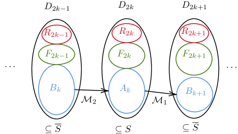
Figure 1: An illustration of a few neighboring layers. Note that $(B_{k},R_{2k-1},F_{2k-1})$ form a partition of odd layer $D_{2k-1}\subseteq\bar{S}$, and $(A_{k},R_{2k},F_{2k})$ form a partition of even layer $D_{2k}\subseteq S$.

Elements can change their types from fresh $\to$ selected $\to$ removed, but never in the other direction. Initially, we start with all elements being fresh. For convenience, we also define “imaginary” layers $D_{0}$ and $D_{2\ell+2}$ with $A_{0}=R_{0}=F_{0}=D_{0}=A_{\ell+1}=R_{2\ell+2}=F_{2\ell+2}=D_{2\ell+2}=\emptyset$. The algorithm maintains the following phase invariants (which are initially satisfied) during the refinement process:

Definition 15 (Phase Invariants, from [CLS⁺19, Section 6.3.2]).

The phase invariants are:

(a-b)

$\Phi_{\ell}=(B_{1},A_{1},B_{2},\ldots,A_{\ell},B_{\ell+1})$ forms a partial augmenting set.

(c)

For $1\leq k\leq\ell$, for any $X\subseteq B_{k+1}+F_{2k+1}=D_{2k+1}-R_{2k+1}$, if $S-(A_{k}+R_{2k})+X\in\mathcal{I}_{1}$ then $S-A_{k}+X\in\mathcal{I}_{1}$.

(d)

$\operatorname{rk}_{2}(W+R_{2k-1})=\operatorname{rk}_{2}(W)$ where $W=S-(D_{2k}-R_{2k})+B_{k}$.

Remark 16.

Invariant (c) essentially says that if $R_{2k+1}$ is “useless”, then so is $R_{2k}$. Similarly, Invariant (d) says that if $R_{2k}$ is “useless”, then so is $R_{2k-1}$. Together they imply that we can safely ignore all the removed elements.

Lemma 17.

Suppose that (i) the phase invariants hold; (ii) $|B_{1}|=|A_{1}|=\cdots=|B_{\ell+1}|$; and (iii) $B_{1}$ is a maximal subset of $D_{1}\setminus R_{1}$ satisfying $S+B_{1}\in{\mathcal{I}}_{1}$. Then $(B_{1},A_{1},\ldots,B_{\ell+1})$ is a maximal augmenting set.

Proof idea..

(See [CLS⁺19, Proof of Lemma 44] for a complete proof). If it was not maximal, there exists an augmenting path $(b_{1},a_{1},\ldots,b_{\ell+1})$ in the exchange graph after augmenting along $(B_{1},A_{1},\ldots,B_{\ell+1})$. However, (iii) then says that $b_{1}$ must have been removed since it cannot be fresh. But if $b_{1}$ is removed, then so was $a_{1}$, then so was $b_{2}$ etc., by invariants (c) and (d) (this requires a technical, but straightforward, argument). However, $b_{\ell+1}$ cannot have been removed (by invariant (d)), which gives the desired contradiction. ∎

3.1.1 Refining Two Adjacent Layers

We now present the basic refinement procedures from [CLS⁺19], which are operations on neighboring layers. There is some asymmetry in how (odd, even) and (even, odd) layer-pairs are handled, arising from the inherent asymmetry of the independence query between $S$ and $\bar{S}$, but the ideas are the same.

$\texttt{RefineAB}(k)$

extends $B_{k+1}$ as much as possible while respecting invariant (a-b) (Lines 1-2). Then a maximal collection of element in $A_{k}$ which can be “matched” to $B_{k+1}$ is found, and the others elements in $A_{k}$ are removed (Lines 3-4).

$\texttt{RefineBA}(k)$

finds a maximal subset $B_{k}$ that can be “matched” to $A_{k}+F_{2k}$, and removes the other elements of $B_{k}$ (Lines 1-2). Then $A_{k}$ is extended with elements from $F_{2k}$ which are the endpoints of the above “matching” (Lines 3-4).

Algorithm 1 $\texttt{RefineAB}(k)$ (called Refine1 in [CLS⁺19, Algorithm 9])

1:Find maximal $B\subseteq F_{2k+1}$ s.t. $S-A_{k}+B_{k+1}+B\in\mathcal{I}_{1}$

2:$B_{k+1}\longleftarrow B_{k+1}+B,F_{2k+1}\longleftarrow F_{2k+1}-B$

3:Find maximal $A\subseteq A_{k}$ s.t. $S-A_{k}+B_{k+1}+A\in\mathcal{I}_{1}$

4:$A_{k}\longleftarrow A_{k}-A,R_{2k}\longleftarrow R_{2k}+A$

Algorithm 2 $\texttt{RefineBA}(k)$ (called Refine2 in [CLS⁺19, Algorithm 10])

1:Find maximal $B\subseteq B_{k}$ s.t. $S-(D_{2k}-R_{2k})+B\in\mathcal{I}_{2}$

2:$R_{2k-1}\longleftarrow R_{2k-1}+B_{k}\backslash B,B_{k}\longleftarrow B$

3:Find maximal $A\subseteq F_{2k}$ s.t. $S-\left(D_{2k}-R_{2k}\right)+B_{k}+A\in\mathcal{I}_{2}$

4:$A_{k}\longleftarrow A_{k}+F_{2k}\backslash A,F_{2k}\longleftarrow A$

The following properties of the RefineAB and RefineBA methods are proven in [CLS⁺19].

Lemma 18 (from [CLS⁺19, Lemmas 40-42]).

Both RefineAB and RefineBA preserve the invariants. Also: after $\texttt{RefineAB}(k)$ is run, we have $|A_{k}|=|B_{k+1}|$ (unless $k=0$). After $\texttt{RefineBA}(k)$ is run, we have $|B_{k}|=|A_{k}|$ (unless $k=\ell+1$).

Lemma 19 (from [CLS⁺19, Lemma 45]).

RefineAB can be implemented with $O(|D_{2k}|+|D_{2k+1}|)$ queries. RefineBA can be implemented with $O(|D_{2k-1}|+|D_{2k}|)$ queries.

Observation 20.

Lemma 18 is particularly interesting. It says that at least $|A^{old}_{k}|-|B^{old}_{k+1}|$ (respectively $|B^{old}_{k}|-|A^{old}_{k}|$) elements change type when running RefineAB (respectively RefineAB).

Remark 21.

20 is used in [CLS⁺19] to bound the number of times one needs to refine the partial augmenting set. Indeed, every element can only change its type a constant number of times. In a single refinement pass, procedures RefineAB(k) and RefineBA(k) are called for all $k$, and we obtain a telescoping sum guaranteeing us that $|B^{old}_{1}|-|B^{old}_{\ell+1}|$ elements have changed their types. Hence, after $O(\sqrt{n})$ refinement passes we have $|B_{1}|-|B_{\ell+1}|\leq\sqrt{n}$, and we are “close” to having a maximal augmenting set—only around $\sqrt{n}$ many augmenting paths away. This is essentially what lets [CLS⁺19] obtain their subquadratic ${\tilde{O}}(n^{1.5}/\text{poly}(\varepsilon))$ algorithm.

3.1.2 Refining Three Adjacent Layers

We are now ready to present the new RefineABA method (Algorithm 3), which is not present in [CLS⁺19]. This method works similarly to RefineAB and RefineBA, but on three (instead of two) consecutive layers $(D_{2k},D_{2k+1},D_{2k+2})$ with the corresponding sets $(A_{k},B_{k+1},A_{k+1})$.

The motivation for this new procedure is that we can get a stronger version of 20: after running $\texttt{RefineABA}(k)$ we want that at least $|A^{old}_{k}|-|A^{old}_{k+1}|$ element in even layers have changed types. Note that there are at most $|S|\leq r$ elements in the even layers (as opposed to $n$ elements in total, which can be much larger), so this means we need to refine the partial augmenting set fewer times when using RefineABA compared to when just using RefineAB and RefineBA. In particular, we will get that after $O(\sqrt{r})$ refinement passes, $|B_{1}|-|B_{\ell+1}|\leq\sqrt{r}$.

Remark 22.

A natural question to ask is if it actually could be the case that only elements in odd layers (i.e. those in $\bar{S}$ which there are up to $n$ many of) change their type (while elements in even layers do not) during the refinement passes in the algorithm of [CLS⁺19] (which only uses the two-layer refinement procedures)? That is, is the new three-layer refinement procedure necessary? The answer is yes. Consider for example the case with 5 layers $B_{1}\subseteq D_{1};A_{1}\subseteq D_{2};B_{2}\subseteq D_{3};A_{2}\subseteq D_{4};B_{3}\subseteq D_{5}$ where $q:=|B_{1}|=|A_{1}|$ and $|A_{2}|=|B_{3}|=0$. Refining the consecutive pair $(B_{1},A_{1})$ or $(A_{2},B_{3})$ will not do anything. When refining $(A_{1},B_{2})$ it could be the case that only $B_{2}$ increases (say any $q$-size subset in $D_{3}$ can be “matched” with $A_{1}$). Similarly, when refining $(B_{2},A_{2})$ it could be the case that only $B_{2}$ decreases (say there is only a single element in $D_{3}$ which could be “matched” with anything in the next layer $D_{4}$, then it is unlikely that this specific element is already selected in $B_{2}$). In this case, we would need to run the two-layer refinement procedures around $|D_{3}|/q\approx n/q$ times before anything other than $B_{2}$ changes. In contrast, the new RefineABA method would, when run on $(A_{1},B_{2},A_{2})$, terminate with $|A_{1}|=|B_{2}|=|A_{2}|$ (that is it would have found the “special” element in $D_{3}$ the first time it is run).

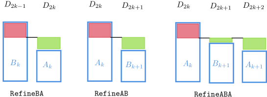
Figure 2: An illustration how the different refine methods change the partial augmenting sets. Newly selected elements are marked in green, while newly removed elements are marked in red.

To explain how RefineABA works, let us start with a simple case, namely when $S=\emptyset$, i.e. there is only one layer between $s$ and $t$ in the exchange graph. Here, finding a maximal augmenting set is the same as finding some maximal set $B$ which is independent in both matroids. Running RefineAB would extend this $B$ with elements as long as it is independent in the first matroid (ignoring the second matroid), while RefineBA would throw away elements from $B$ until it is independent in the second matroid (now ignoring the first matroid). If we just alternate running RefineAB and RefineBA we would in the worst case need to do this up to $n$ times (which is too expensive). Instead, there is a very simple greedy algorithm that efficiently finds a maximal set $B$ independent in both of the matroids: for each element, include it in $B$ if this does not break independence for either matroid. This is akin to how our RefineABA method works: it looks at the constraints from both matroids simultaneously (both neighboring layers) and greedily selects $B$.

In the general case, RefineABA can be seen as running RefineAB and RefineBA simultaneously. The algorithm starts by asserting $|B_{k+1}|=|A_{k+1}|$ (so that $S+B_{k+1}-A_{k+1}\in{\mathcal{I}}_{2}$) by running RefineBA. So now we have both $S+B_{k+1}-A_{k}\in{\mathcal{I}}_{1}$ and $S+B_{k+1}-A_{k+1}\in{\mathcal{I}}_{2}$, and the algorithm proceeds to greedily extend $B_{k+1}$ while it is still consistent with both the previous layer $A_{k}$ and the next layer $A_{k+1}+F_{2k+2}$. Some care has to be taken here to also mark elements as removed to preserve the phase invariants. Finally, the algorithm decreases the size of $A_{k}$, respectively increases the size of $A_{k+1}$, to both match $|B_{k+1}|$.

Algorithm 3 $\texttt{RefineABA}(k)$

1:$\texttt{RefineBA}(k+1)$

2:for $x\in F_{2k+1}$ do

3:     if $S-A_{k}+B_{k+1}+x\in{\mathcal{I}}_{1}$ then

4:         if $S-A_{k+1}-F_{2k+2}+B_{k+1}+x\in{\mathcal{I}}_{2}$ then

5:              $B_{k+1}\leftarrow B_{k+1}+x,\quad F_{2k+1}\leftarrow F_{2k+1}-x$ $\triangleright$ Select $x$

6:         else

7:              $R_{2k+1}\leftarrow R_{2k+1}+x,\quad F_{2k+1}\leftarrow F_{2k+1}-x$ $\triangleright$ Remove $x$               

8:$\texttt{RefineBA}(k+1)$

9:$\texttt{RefineAB}(k)$

We now state some properties of RefineABA. These properties are relatively straightforward—although technical and notation-heavy—to prove.

Lemma 23.

RefineABA$(k)$ preserves the phase invariants.

Lemma 24.

After RefineABA$(k)$ is run, we have $|A_{k}|=|B_{k+1}|=|A_{k+1}|$ (unless $k=0$ or $k=\ell$, where the sets $A_{0}=A_{\ell+1}=\emptyset$ are “imaginiary”).

Lemma 25.

RefineABA$(k)$ uses $O(|D_{2k}|+|D_{2k+1}|+|D_{2k+2}|)$ independence queries.

Proof of Lemma 23.

Intuitively, the only tricky part is showing that invariant (c) is preserved when some $x$ is removed in line 7. We can pretend that we add $x$ to $B_{k+1}$ temporarily, and then run $\texttt{RefineBA}(k+1)$ in a way which would remove this $x$ immediately (and thus removing $x$ did indeed preserve the invariants). We present a formal proof below.

We already know that RefineAB and RefineBA preserve the invariants by Lemma 18, so it suffices to check that the for-loop starting in line 2 preserves the invariants. We verify that this is the case after processing each $x\in F_{2k+1}$ in the for-loop:

Invariant (a-b)

holds by design: when $x$ is added to $B_{k+1}$ we know both that $S-A_{k}+B_{k+1}+x\in{\mathcal{I}}_{1}$ and $\operatorname{rk}_{2}(S-A_{k+1}+B_{k+1})$ cannot decrease. Note also that $\operatorname{rk}_{2}(S-A_{k+1}+B_{k+1})\leq\operatorname{rk}_{2}(S)$ when $k+1\leq\ell$ too (so it cannot increase either), since otherwise there must exist some $b\in B_{k+1}$ so that $S+b\in{\mathcal{I}}_{2}$ (by the matroid exchange property) which is impossible since we are not in the last layer (the layer preceding $t$ in $G(S)$).

Invariant (c)

trivially holds, since the set $B_{k+1}+F_{2k+1}$ will only decrease, which only restricts the choice of $X\subseteq B_{k+1}+F_{2k+1}$.

Invariant (d)

will also be preserved. We need to argue that this is the case when $x$ is removed in line 7. Let $W:=S-A_{k+1}-F_{2k+2}+B_{k+1}=S-(D_{2k+2}-R_{2k+2})+B_{k+1}$, and $R^{old}_{2k+1}$ be the set $R_{2k+1}$ before $x$ was added to it. First note that $W\in{\mathcal{I}}_{2}$, since this holds after the RefineBA call in line 1, (since $|A_{k+1}|=|B_{k+1}|$ after this call) and $B_{k+1}$ is only extended with elements which preserve this property. This means that $\operatorname{rk}_{2}(W+x)=\operatorname{rk}_{2}(W)=|W|$, since $W+x=S-A_{k+1}-F_{2k+2}+B_{k+1}+x\notin{\mathcal{I}}_{2}$. Since the invariant held before, we also know that $\operatorname{rk}_{2}(W+R^{old}_{2k+1})=\operatorname{rk}_{2}(W)=|W|$. Hence $W$ is a maximal independent (in ${\mathcal{M}}_{2}$) subset of $W+R^{old}_{2k+1}+x$, as neither $x$ nor elements from $R^{old}_{2k+1}$ can be used to extend it. Hence $\operatorname{rk}_{2}(W+R^{old}_{2k+1}+x)=|W|=\operatorname{rk}_{2}(W)$; that is invariant (d) is preserved. ∎

Proof of Lemma 24.

We focus our attention on the RefineBA and RefineAB calls in lines 8-9, and argue that they do not change $B_{k+1}$. This would prove the lemma, since by Lemma 18 we would then have $|A_{k}|=|B_{k+1}|$ and $|B_{k+1}|=|A_{k+1}|$.

Indeed, $\texttt{RefineBA}(k+1)$ finds a maximal $B\subseteq B_{k+1}$ such that $S-(D_{2k+2}-R_{2k+2})+B\subseteq{\mathcal{I}}_{2}$, and remove all elements not in $B$ from $B_{k+1}$. Here, $B=B_{k+1}$ will be found, since $S-(D_{2k+2}-R_{2k+2})+B_{k+1}\in{\mathcal{I}}_{2}$ after the for-loop in line 2 of RefineABA.

Similarly, we see that $\texttt{RefineAB}(k)$ finds a maximal $B\subseteq F_{2k+1}$ such that $S-A_{k}+B_{k+1}+B\in{\mathcal{I}}_{1}$, and extend $B_{k+1}$ with this $B$. However, only $B=\emptyset$ works, since each $x\in F_{2k+1}$ for which $S-A_{k}+B_{k+1}+x\in{\mathcal{I}}_{1}$ was either selected or removed in lines 5 or 7. ∎

Proof of Lemma 25.

RefineAB$(k)$ uses $O(|D_{2k}|+|D_{2k+1}|)$ queries, and RefineBA$(k+1)$ uses $O(|D_{2k+1}|+|D_{2k+2}|)$ queries. The for-loop in line 2 will use $O(|D_{2k+1}|)$ queries. ∎

3.1.3 Refinement Pass

We can now present the full Refine method (Algorithm 4), which simply scans over the layers and calls RefineABA on them. Our Refine is a modified version of Refine from [CLS⁺19, Algorithm 11] using our new RefineABA method instead of just RefineAB and RefineBA. Just replacing the Refine method in the final algorithm of [CLS⁺19] with our modified Refine below leads to an ${\tilde{O}}(n\sqrt{r}/\varepsilon^{1.5})$-query algorithm (compared to their ${\tilde{O}}(n^{1.5}/\varepsilon^{1.5})$), and concludes our first improvement (as discussed in Item 1 in Section 1.1).

Algorithm 4 $\texttt{Refine}(k)$

1:for $k=\ell,\ \ell-1,\ \ell-2,\ \ldots,\ 1,\ 0$ do

2:     RefineABA(k)

The following Lemma 26 will be useful to bound the number of Refine calls needed in our final algorithm, and closely corresponds to [CLS⁺19, Corollary 43]. Our Refine implementation has the advantage that it only counts the elements in the even layers, of which there are at most $r$.

Lemma 26.

Let $(B^{old}_{1},A^{old}_{1},\ldots)$ and $(B^{new}_{1},A^{new}_{1},\ldots)$ be the sets before and after Refine is run. Then at least $|B^{new}_{1}|-|B^{new}_{\ell+1}|$ elements in even layers have changed types.

Proof.

Note that whenever $A_{k}$ changes, it is because some elements changed it types in $D_{2k}$. In particular, if the size of $A_{k}$ increases (respectively decreases) by $z$, at least $z$ elements will change types from fresh to selected (respectively from selected to removed) in $D_{2k}$.

After the first iteration $|A_{\ell}|=|B^{new}_{\ell+1}|$, so at least $|A^{old}_{\ell}|-|B^{new}_{\ell+1}|$ elements in $D_{2\ell}$ changed types. Similarly, after the iteration when $k=i$ (for $1\leq i\leq\ell-1$), $|A_{i}|=|A_{i+1}|$, and hence at least $|A^{old}_{i}|-|A_{i}|$ elements in $D_{2i}$ changed types plus at least $|A_{i+1}|-|A^{old}_{i+1}|$ elements in $D_{2i+2}$ changed types. Finally, after the last iteration $|A_{1}|=|B^{new}_{1}|$, and hence at least $|B^{new}_{1}|-|A^{old}_{1}|$ elements in $D_{2}$ changed types.

The above terms telescope, and we conclude that at least $|B^{new}_{1}|-|B^{new}_{\ell+1}|$ elements in the even layers changed its types when Refine was run. ∎

Lemma 27.

Refine uses $O(n)$ independence queries.

Proof.

This follows directly by Lemma 25. ∎

3.2 Refining Along a Path

If we just run Refine until we get a maximal augment set (i.e. until $|B_{1}|=|B_{\ell+1}|$) we need to potentially run Refine as many as $\Theta(r)$ times, which needs too many independence queries. Lemma 26 tells us that Refine makes the most “progress” while $|B_{1}|-|B_{\ell+1}|$ is large: in fact, only $O(r/p)$ calls to Refine is needed until $|B_{1}|-|B_{\ell+1}|\leq p$. The idea in [CLS⁺19] is thus to stop refining when $|B_{1}|-|B_{\ell+1}|$ is small enough and fall back to finding augmenting paths one at a time (they prove that one needs to find at most $O((|B_{1}|-|B_{\ell+1}|)\ell)$ many). We use a similar idea in that we swap to a different procedure when $|B_{1}|-|B_{\ell+1}|$ is small enough, the difference being that we still work with the partial augmenting set. This will let us show that only $O(|B_{1}|-|B_{\ell+1}|)$ many “paths” need to be found, saving a factor $\ell\approx\frac{1}{\varepsilon}$ compared to [CLS⁺19].

This section thus describes the second improvement (as discussed in Item 2 in Section 1.1). Note that this improvement is independent of the first improvement (i.e. the three-layer refine). We aim to prove the following lemma.

Lemma 28.

There exists a procedure (RefinePath, Algorithm 5), which uses $O(n\log r)$ independence queries, preserves the invariants, and either:

1. Increases the size of $B_{\ell+1}$ by at least $1$.

2. Terminates with $(B_{1},A_{1},\ldots,B_{\ell+1})$ being a maximal augmenting set.

RefinePath attempts to find what we call a valid path. What we want is a sequence of elements which we can add to the partial augmenting set without violating the invariants and the properties of the partial augmenting set. It turns out (not very surprisingly) that such sequences of elements can be characterized by a notion of paths in something which resembles the exchange graph with respect to our partial augmenting set. This is what motivates the definition of valid paths below.

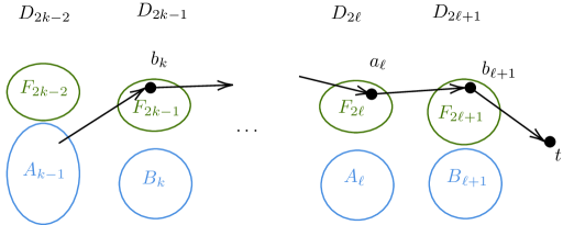
Figure 3: A valid path $(b_{k},\ldots,a_{\ell},b_{\ell+1},t)$ “starting” from the partial augmenting set at $A_{k-1}$, so that we can use Lemma 31 and augment along it.

Definition 29 (Valid path).

A sequence $(b_{i},a_{i},b_{i+1},\ldots,b_{\ell+1},t)$ (or $(a_{i},b_{i+1},\ldots,b_{\ell+1},t)$) is called a valid path (with respect to the partial augmenting set) if for all $k\geq i$:

1. $a_{k}\in F_{2k}$ and $b_{k}\in F_{2k-1}$.

2. $S+B_{\ell+1}+b_{\ell+1}\in{\mathcal{I}}_{2}$.

3. $S-A_{k}+B_{k}-a_{k}+b_{k}\in{\mathcal{I}}_{2}$.

4. $S-A_{k}+B_{k+1}-a_{k}+b_{k+1}\in{\mathcal{I}}_{1}$.

Remark 30.

Compare the properties of valid paths with the edges in the exchange graph from Definition 6. A valid path is essentially a path in the exchange graph after we have already augmented $S$ by our partial augmenting set (even though this exchange graph is not exactly defined, since it is not guaranteed that $S$ remains a common independent set when augmented by a partial augmenting set).

Lemma 31.

If $p=(b_{i},a_{i},b_{i+1},\ldots,b_{\ell+1},t)$ is a valid path starting at $b_{i}$, such that $S-A_{i-1}+B_{i}+b_{i}\in{\mathcal{I}}_{1}$, then $(B_{1},A_{1},\ldots,B_{i-1},A_{i-1},\ B_{i}+b_{i},A_{i}+a_{i},\ldots,B_{\ell+1}+b_{\ell})$ is a partial augmenting set satisfying the invariants.

Proof.

That it forms a partial augmenting set is true by the definition of valid paths, and the fact that $S-A_{i-1}+B_{i}+b_{i}\in{\mathcal{I}}_{1}$. Indeed, it cannot be the case that $|A_{i-1}|<|B_{i}+b_{i}|$ when $i>1$, since then $\operatorname{rk}_{1}(S-A_{i-1}+B_{i}+b_{i})>|S|=\operatorname{rk}_{1}(S)$ implies that some element $x\in(B_{i}+b_{i})$ satisfies $S+x\in{\mathcal{I}}_{1}$ (i.e. it is in the first layer $D_{1}$) by the exchange property of matroids. Invariants (c) and (d) are trivially true since the sets $A_{k}$ and $B_{k}$ are only extended. ∎

The goal of RefinePath (Algorithm 5) is thus to find a valid path satisfying the conditions in Lemma 31. Towards this goal, RefinePath will start from the last layer $D_{2\ell+1}$ and “scan left” in a breadth-first-search manner while keeping track of valid paths starting at each fresh vertex $x$ (the next element on such a path will be stored as $\texttt{next}[x]$). If at some point one valid path can “enter” the partial augmenting set in a layer, we are done and can use Lemma 31. We also show that it is safe (i.e. preserves the invariants) to remove all the fresh elements $x$ for which we cannot find a valid path starting at $x$.

To efficiently find the “edges” during our breadth-first-search using only independence-queries, we use the binary-search trick from Lemma 9. However, this relies on the partial augmenting set being locally “flat” in the layers we are currently exploring, i.e. $|B_{k}|=|A_{k}|$ respectively $|B_{k}|=|A_{k+1}|$. We can ensure this by running RefineAB respectively RefineBA while performing the scan.

Now we are ready to present the pseudo-code of the RefinePath method (Algorithm 5). Due to the asymmetry between even/odd layers and independence queries, we need to handle moving from layer $B$ to $A$ and from $A$ to $B$ a bit differently, but the ideas are similar.

Algorithm 5 RefinePath

1:for $k=\ell+1,\ \ell,\ \ldots,\ 2,\ 1$ do $\triangleright$ Process $(B_{k},A_{k})$

2:     $\texttt{RefineBA}(k)$

3:     if some element $a$ was added to $A_{k}$ in the above refine-call then

4:         Add the valid path starting at $\texttt{next}[a]$ to the partial augmenting set

5:         return      

6:     for each element $b\in F_{2k-1}$ do

7:         if $S-A_{k}-F_{2k}+B_{k}+b\notin{\mathcal{I}}_{2}$ then

8:              Remove $b$, that is: $F_{2k-1}\leftarrow F_{2k-1}-b,\quad R_{2k-1}\leftarrow R_{2k-1}+b$

9:         else

10:               Find an $a\in F_{2k}$ such that $S-A_{k}+B_{k}+b-a\in{\mathcal{I}}_{2}$. Let $\texttt{next}[b]=a$.

11:              (Or, if $k=\ell+1$, just let $\texttt{next[b]}=t$)               

12:$\triangleright$ Process $(A_{k-1},B_{k})$

13:     if some element $b\in F_{2k-1}$ satisfies $S-A_{k-1}+B_{k}+b\in{\mathcal{I}}_{1}$ then

14:         Add the valid path starting at $b$ to the partial augmenting set.

15:         return      

16:     $\texttt{RefineAB}(k-1)$

17:     $Q\leftarrow F_{2k-2}$.

18:     for each element $b\in F_{2k-1}$ do

19:         while can find $a\in Q$ such that $S-A_{k-1}+B_{k}+b-a\in{\mathcal{I}}_{1}$ do

20:              $Q\leftarrow Q-a$. Let $\texttt{next}[a]=b$.               

21:     Remove all elements in $Q$, that is: $F_{2k-2}\leftarrow F_{2k-2}-Q,\quad R_{2k-2}\leftarrow R_{2k-2}+Q$.

22:

23:If we reached here, $(B_{1},A_{1},\ldots,B_{\ell+1})$ is a maximal augmenting set.

lemmaPATHinv RefinePath preserves the invariants.

Proof.

The proof is relatively straightforward, but technical. The only non-trivial part is showing that invariants (c) and (d) are preserved after we remove something in line 8 or line 21. Intuitively, if we remove $b$ in line 8, we can instead think of temporarily adding $b$ to $B_{k}$ and running $\texttt{RefineBA}(k)$ in such a way so that $b$ is immediately removed. A similar intuitive argument works for line 21. We next present a formal proof.

We know that RefineAB and RefineBA preserve the invariants, by Lemma 18. We also know by Lemma 31 that adding a valid path to the partial augmenting set also preserves the invariants. So what remains is to show that the invariants are preserved after:

Line 8.

We only need to check invariant (d), the other ones trivially hold. Let $W=S-A_{k}-F_{2k}+B_{k}=S-(D_{2k}-R_{2k})+B_{k}$ and $R^{old}_{2k-1}$ be $R_{2k-1}$ before $b$ was added to it. Note that $b$ is such that $W+b\notin{\mathcal{I}}_{2}$, and we know that $W\subseteq S-A_{k}+B_{k}\in{\mathcal{I}}_{2}$ and hence $\operatorname{rk}_{2}(W+R^{old}_{2k-1})=\operatorname{rk}_{2}(W)=|W|$ and $\operatorname{rk}_{2}(W+b)=\operatorname{rk}_{2}(W)=|W|$. We thus need to show that $\operatorname{rk}_{2}(W+R^{old}_{2k-1}+b)=|W|$ too, which is clear since $W$ is a maximal independent subset of $W+R^{old}_{2k-1}+b$ (it can neither be extended with elements from $R^{old}_{2k-1}$ nor with $b$).

Line 21.

We only need to check invariant (c), the other ones trivially hold. We imagine we add the $a\in Q$ to $R_{2k-2}$ one-by-one, and show that the invariant (c) is preserved after each such addition. So consider some $a\in Q$ which will be removed, and let $R^{old}_{2k-2}$ be the set $R_{2k-2}$ just before we added $a$ to it. First note that $\operatorname{rk}_{1}(S-A_{k-1}+B_{k}+F_{2k-1}-a)=\operatorname{rk}_{1}(S-A_{k-1}+B_{k}+F_{2k-1})-1=|S-A_{k-1}+B_{k}|-1$, as otherwise there must exist some $b\in F_{2k-1}$ such that $S-A_{k-1}+B_{k}+b-a\in{\mathcal{I}}_{1}$ (by the matroid exchange property), and $a$ would have been discovered in line 19 and therefore been removed from $Q$. So the “return” of adding $a$ to $S-A_{k-1}+B_{k}+F_{2k-1}-a$ is increasing the rank by $1$. Now consider some arbitrary $X\subseteq B_{k}+F_{2k-1}$ such that $S-A_{k-1}+X-R^{old}_{2k-2}-a\in{\mathcal{I}}_{1}$. We need to show that $S-A_{k-1}+X\in{\mathcal{I}}_{1}$. Note that $S-A_{k-1}+X-R^{old}_{2k-2}-a\subseteq S-A_{k-1}+B_{k}+F_{2k-1}-a$. Hence, by the diminishing returns (of adding $a$) we know $\operatorname{rk}_{1}(S-A_{k-1}+X-R^{old}_{2k-2})\geq\operatorname{rk}_{1}(S-A_{k-1}+X-R^{old}_{2k-2}-a)+1=|S-A_{k-1}+X-R^{old}_{2k-2}|$, or equivalently that $S-A_{k-1}+X-R^{old}_{2k-2}\in{\mathcal{I}}_{1}$. Since the invariant held before, we conclude that $S-A_{k-1}+X\in{\mathcal{I}}_{1}$ too, which finishes the proof. ∎

Valid paths.

The algorithm keeps track of a valid path starting at each fresh vertex it has processed. That is, after processing layer $D_{k}$, all elements in $F_{k}$ must be the beginning of a valid path, else they were removed. In particular, the algorithm remembers the valid path starting at $x$ as $(x,\texttt{next}[x],\texttt{next}[\texttt{next}[x]],\ldots)$. It is easy to verify that this sequence does indeed satisfy the conditions of valid paths by inspecting lines 10 and 19.

We also discuss what happens when the algorithm chooses to add a valid path to the partial augmenting set (i.e. in line 4 or 14). If we are in Line 14, we can directly apply Lemma 31. Say we instead are in Line 4, and some $a$ which was previously fresh has been added to $A_{k}$. The RefineBA call can only have increased $A_{k}$ (that is $A_{k}\supseteq A^{old}_{k}+a)$, so $S-A_{k}+B_{k+1}+b\in{\mathcal{I}}_{1}$ will holds for $b=\texttt{next}[a]$ and we can apply Lemma 31 here too.

When no path is found.

In the case when no valid path to add to the partial augmenting set is found, RefinePath must terminate with $|B_{1}|=|A_{1}|=\cdots=|B_{\ell+1}|$. This is because the RefineAB and RefineBA will never select any new elements. That is RefineBA will not change $A_{k}$ (as otherwise we enter the if-statement at line 4), and RefineAB will not change $B_{k}$ (since if $b\in F_{2k-1}$ with $S-A_{k-1}+B_{k}+b\in{\mathcal{I}}_{1}$ existed we would have entered the if-statement at line 14). We also remark that RefinePath ends with $B_{1}$ being a maximal subset of $D_{1}\setminus R_{1}$, as otherwise some $b$ would have been found in line 13. Hence Lemma 17 implies that $(B_{1},A_{1},\ldots,B_{\ell+1})$ now forms a maximal augmenting set.

Query complexity.

The RefineAB and RefineBA calls will in total use $O(n)$ queries. The independence checks at Lines 7 and 13 happens at most once for each element, and thus use $O(n)$ queries in total. Lines 10 and 19 can be implemented using the binary-search-exchange-discovery Lemma 9. Hence Line 10 will use, in total, $O(n\log r)$ queries and Line 19 will use, in total, $O(n\log r)$ queries (since each $a\in Q$ will be discovered at most once). So we conclude that Algorithm 5 uses $O(n\log r)$ independence queries.

3.3 Hybrid Algorithm

Now we are finally ready to present the full algorithm of a phase, which is parameterized by a variable $p$. The following algorithm is similar to that of [CLS⁺19, Algorithm 12] but uses our improved Refine method and finds individual paths using the RefinePath method.

Algorithm 6 Phase $\ell$

1:Calculate the distance layers by a BFS.

2:Run Refine (Algorithm 4) until $|B_{1}|-|B_{\ell+1}|\leq p$, but at least once.

3:Run RefinePath (Algorithm 5) until $(B_{1},A_{1},\ldots B_{\ell+1})$ is maximal. Augment along it.

Lemma 32.

Except for line 1, Algorithm 6 uses $O(nr/p+np\log r)$ queries.

Proof.

Lemma 26 tells us that Refine changes types of at least $p$ elements in even layers (i.e. elements in $S$) every time it is run, except maybe the last time. Thus we only run Refine $O(|S|/p+1)$ times. Each call takes $O(n)$ queries (Lemma 27), for a total of $O(nr/p)$ queries in line 2 of the algorithm.

Now we argue that $B_{1}$ can never become larger than what it was just after line 2 was run. This is because Refine will run at least once, and ends with a $\texttt{RefineABA}(0)$ call which in turn ends with a RefineAB(0) call—which extends $B_{1}$ to be a maximal set in $D_{1}\setminus R_{1}$ for which $S+B_{1}\subseteq{\mathcal{I}}_{1}$ holds.

Lemma 28 tells us that each (except the last) time RefinePath is run, $B_{\ell+1}$ increases by $1$. This can happen at most $p$ times, so line 3 uses a total of $O(np\log r)$ queries. ∎

Now it is easy to prove Section 1, which we restate below.

*

Proof.

Pick $p=\sqrt{r/\log r}$. Then each phase will use $O(n\sqrt{r\log r})$ independence queries (by Lemma 32), plus a total of $O(\frac{1}{\varepsilon}n\log r)$ to run the BFS’s across all phases (see [CLS⁺19] for details on the BFS implementation). Since we need only run $O(\frac{1}{\varepsilon})$ phases (by Lemma 8 and Theorem 14), in total the algorithm will use $O(\frac{1}{\varepsilon}n\sqrt{r\log r})$ queries. ∎

4 Exact Matroid Intersection

In this section, we prove Section 1 (restated below) by showing how our improved approximation algorithm leads to an improved exact algorithm when combined with the algorithms of [BvdBMN21].

*

Approximation algorithms are great at finding the many, very short augmenting paths efficiently. Blikstad-v.d.Brand-Mukhopadhyay-Nanongkai [BvdBMN21, Algorithm 2] very recently showed how to efficiently find the remaining few, very long augmenting paths, with a randomized algorithm using ${\tilde{O}}(n\sqrt{r})$ queries per augmentation (or, with a slightly less efficient deterministic algorithm using ${\tilde{O}}(nr^{2/3})$ queries). In the randomized ${\tilde{O}}(n^{6/5}r^{3/5})$-query exact algorithm of [BvdBMN21, Algorithm 3], the current bottleneck is the approximation algorithm used. Replacing the use of the ${\tilde{O}}(n^{1.5}/\varepsilon^{1.5})$-query approximation algorithm from [CLS⁺19] with our improved version we obtain the more efficient randomized ${\tilde{O}}(nr^{3/4})$-query Algorithm 7.

Algorithm 7 Exact Matroid Intersection (Modified version of [BvdBMN21, Algorithm 3])

1:Run the approximation algorithm (Section 1) with $\varepsilon=r^{-1/4}$ to obtain a common independent set $S$ of size at least $(1-\varepsilon)r=r-r^{3/4}$.

2:Starting with $S$, run Cunningham’s algorithm (as implemented by [CLS⁺19]), until the distance between $s$ and $t$ becomes larger than $r^{3/4}$.

3:Keep finding augmenting paths—one at a time—to augment along, using the randomized $O(n\sqrt{r}\log n)$-query algorithm of [BvdBMN21, Algorithm 2]. When no $(s,t)$-path can be found in the exchange graph, $S$ is a largest common independent set.

Query complexity.

We analyse the individual lines of Algorithm 7.

Line 1.

We see that the approximation algorithm uses $O(nr^{3/4}\log n)$ queries in line 1.

Line 2.

One need to (i) compute distances up to $d=r^{3/4}$, and (ii) perform at most $O(r^{3/4})$ augmentations. [CLS⁺19, BvdBMN21, Ngu19] show how to do (i) in $O(nd\log n)=O(nr^{3/4}\log n)$ queries in total over all phases of Cunningham’s algorithm, and how to do (ii) using $O(n\log n)$ queries per augmentation (for a total of $O(nr^{3/4}\log n)$ queries).

Line 3.

By Lemma 8, line 3 runs $O(r^{1/4})$ times—each using $O(n\sqrt{r}\log n)$ queries—for a total of $O(nr^{3/4}\log n)$ queries.

Remark 33.

In Algorithm 7, the bottleneck between line 1-2 and line 2-3 now matches (which was not the case in [BvdBMN21]). This means that if one wants to improve the algorithm by replacing the subroutines in line 1 and 3, one need to both improve the approximation algorithm (line 1) and the method to find a single augmenting-path (line 3).

References

• [AD71] Martin Aigner and ThomasΒ A. Dowling. Matching theory for combinatorial geometries. Transactions of the American Mathematical Society, 158(1):231–245, 1971.
• [BvdBMN21] Joakim Blikstad, Jan vanΒ den Brand, Sagnik Mukhopadhyay, and Danupon Nanongkai. Breaking the quadratic barrier for matroid intersection. In STOC. ACM, 2021.
• [CLS+19] Deeparnab Chakrabarty, YinΒ Tat Lee, Aaron Sidford, Sahil Singla, and SamΒ Chiu-wai Wong. Faster matroid intersection. In FOCS, pages 1146–1168. IEEE Computer Society, 2019.
• [CQ16] Chandra Chekuri and Kent Quanrud. A fast approximation for maximum weight matroid intersection. In SODA, pages 445–457. SIAM, 2016.
• [Cun86] WilliamΒ H. Cunningham. Improved bounds for matroid partition and intersection algorithms. SIAM J. Comput., 15(4):948–957, 1986.
• [Edm70] Jack Edmonds. Submodular functions, matroids, and certain polyhedra. In Combinatorial structures and their applications, pages 69–87. 1970.
• [Edm79] Jack Edmonds. Matroid intersection. In Annals of discrete Mathematics, volumeΒ 4, pages 39–49. Elsevier, 1979.
• [EDVJ68] Jack Edmonds, GBΒ Dantzig, AFΒ Veinott, and MΒ JΓΌnger. Matroid partition. 50 Years of Integer Programming 1958–2008, page 199, 1968.
• [Law75] EugeneΒ L. Lawler. Matroid intersection algorithms. Math. Program., 9(1):31–56, 1975.
• [LSW15] YinΒ Tat Lee, Aaron Sidford, and SamΒ Chiu-wai Wong. A faster cutting plane method and its implications for combinatorial and convex optimization. In FOCS, pages 1049–1065. IEEE Computer Society, 2015.
• [Ngu19] HuyΒ L. Nguyen. A note on cunningham’s algorithm for matroid intersection. CoRR, abs/1904.04129, 2019.