The Pyrat Bay Framework for Exoplanet Atmospheric Modeling:
A Population Study of Hubble/WFC3 Transmission Spectra

Abstract

https://pyratbay.readthedocs.io) and tested to provide maximum accessibility to the community and long-term development stability.

https://pyratbay.readthedocs.io) and tested to provide maximum accessibility to the community and long-term development stability.

1 Introduction

Since the discovery of the first planet orbiting around a solar-type star other than our sun (Mayor & Queloz, 1995), exoplanets have shaken our conception of the universe. The more than 4000 exoplanets known to date have shown a diversity far larger than what we expected from our own solar system. The unprecedented conditions found in hot-Jupiter or super-Earth planets, for example, represent an invaluable opportunity to widen our understanding of atmospheric and planetary physics. In terms of characterization, spectro-photometric time-series observations of transiting exoplanets have taken a central stage. When planets transit in front of their host stars, they block a fraction of the observed stellar flux. The amplitude of this signal is proportional to the square of the planet-to-star radius ratio. When planets pass behind their host stars, the planetary emission is blocked by the star. The amplitude of this signal is proportional to the planet-to-star flux ratio. The observational and theoretical techniques used to characterize transiting exoplanets have shown a sustained and fast-paced development over time. Characterization studies from space-based observatories (the focus of this article) have quickly evolved from single-target, single-broadband observations (Charbonneau et al., 2000), to population studies of multi-wavelength spectroscopic observations (e.g., Sing et al., 2016; Iyer et al., 2016; Barstow et al., 2017; Fu et al., 2017; Tsiaras et al., 2018; Fisher & Heng, 2018; Pinhas et al., 2019; Welbanks et al., 2019; Garhart et al., 2020), covering from the ultraviolet to the infrared region of the spectrum. By modeling how light interacts with a planetary atmosphere (via the radiative-transfer equation), transit and eclipse observations help us determine the physical properties of the atmosphere, as different species produce unique spectral features as a function of wavelength, temperature, and pressure. Furthermore, the inferred physical state of a planetary atmosphere gives us an insight into the planet’s formation, evolution, chemistry, and dynamics. To estimate the atmospheric properties in a statistically robust manner, many studies adopt the Bayesian retrieval approach. This approach evaluates the posterior distribution of a parametric atmospheric model given a dataset of an observed spectrum. A Bayesian sampler—e.g., a Markov chain Monte Carlo (MCMC, Metropolis et al., 1953) or nested sampling (Skilling, 2004)— explores the parameter space by evaluating a large number of model samples, guided by the prior and likelihood functions. The sampler generates a posterior distribution from which one can obtain the parameters’ best-fitting values and credible intervals (the uncertainties). Madhusudhan & Seager (2009, 2010) introduced the retrieval approach to the exoplanet field for atmospheric characterization. Soon after, other independent retrieval schemes emerged, e.g., NEMESIS (Irwin et al., 2008), SCARLET (Benneke, 2015), POSEIDON (MacDonald & Madhusudhan, 2017), ATMO (Evans et al., 2017; Wakeford et al., 2017a), HyDRA (Gandhi & Madhusudhan, 2018), and ARCiS (Ormel & Min, 2019). Recently, a number of open-source retrieval packages have facilitated the accessibility and cross-comparison of retrieval frameworks, e.g., CHIMERA (Line et al., 2013), PLATON (Zhang et al., 2019), petitRADTRANS (Mollière et al., 2019), Helios-r2 (Kitzmann et al., 2020), and TauREx (Al-Refaie et al., 2019). Developing a comprehensive atmospheric modeling framework is a challenging task, as it requires the knowledge of a vast number of physical processes (e.g., radiative transfer, chemistry, cloud formation, dynamics, etc.) and advanced statistical analyses. Furthermore, both the physical and statistical analyses are computationally intensive tasks, demanding an efficient implementation of tools. To overcome these limitations, researchers resort to a wide range of often strong assumptions and simplifications, for example: adopt 1D atmospheric parameterizations for 3D objects, neglect stellar contamination due to starspots or faculae (e.g., Rackham et al., 2018), or assume isobaric properties throughout the atmosphere (Heng & Kitzmann, 2017). The inadequacy of these assumptions has already been debunked (e.g., Rocchetto et al., 2016; Blecic et al., 2017; Caldas et al., 2019; Welbanks & Madhusudhan, 2019; Welbanks et al., 2019; Taylor et al., 2020; MacDonald et al., 2020). However, the limited signal-to-noise ratio, spectral coverage, and resolving power of current instruments do not statistically justify the use of more sophisticated models. This will not be the case for the next generation of observatories, like the James Webb Space Telescope or the Atmospheric Remote-sensing Infrared Exoplanet Large-survey (Ariel) mission, as they will enable a more precise characterization of planetary atmospheres. The flexibility of the retrieval approach allows for a wide variety of modeling assumptions, ranging from freely-independent parameterizations (where atmospheric properties vary independently of each other) to self-consistent calculations (where the different properties are related through physical principles). In general, more self-consistent models require fewer free parameters, which simplifies the posterior exploration. However, such an approach makes strong assumptions that may not be applicable to a given case. The adopted assumptions can even dominate the outcome of a retrieval study. Thus, it is highly valuable to compare and contrast the results from multiple retrieval frameworks that apply different theoretical and statistical approaches. Only recently the community has started to carry out large-scale cross-validation studies of these retrieval frameworks (Baudino et al., 2017; Barstow et al., 2020) and multiple-independent analyses of a same observation (Kilpatrick et al., 2018; Venot et al., 2020). In this context, where retrieval results are strongly model-dependent and there is a need for analysis intercomparison, we present the Python Radiative-transfer in a Bayesian framework (Pyrat Bay), a modular open-source package for planetary atmospheric modeling, emission and transmission spectral synthesis, and Bayesian atmospheric retrieval. In Section 2, we describe the Pyrat Bay atmospheric modeling and retrieval package. In Section 3 we benchmark the Pyrat Bay package by comparing its outputs to other datasets and open-source packages. In Section 4 we present the Pyrat Bay atmospheric retrieval analysis of transmission spectra for 26 exoplanet datasets obtained from space-based observations. Finally, in Section 5 we summarize our conclusions and discuss future developments.

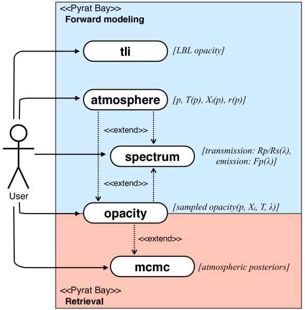
Figure 1: Pyrat Bay Unified Modeling Language (UML) use case diagram, and the main outputs from each case (italics). Users can execute the Pyrat Bay run modes (white bubbles) either individually or chained (dashed lines) in a single command (e.g., compute a temperature profile, abundances, and spectrum all at once), or execute a case with custom inputs provided (e.g., compute a spectrum from a custom provided atmospheric model).

2 The Pyrat-bay Modeling Package

The Python Radiative-transfer in a Bayesian framework (Pyrat Bay) implements state-of-the-art forward and retrieval-modeling tools to sample line-by-line cross sections, computes one-dimensional atmospheric models, generates transmission and emission spectra, and performs Bayesian atmospheric retrievals. Figure 1 shows the current Pyrat Bay running modes available to the user. Briefly, the tli mode reformats cross-section line lists that are available online into transition line information (TLI) files, which is the format used by Pyrat Bay to compute spectra. The atmosphere mode computes atmospheric pressure ($p$), temperature ($T$), volume-mixing-ratio abundance ($X_{\rm i}$), and altitude ($r$) profiles. The spectrum mode computes transmission spectra of stellar light as it passes through the limb of a planet during a transit, or emission spectra of a planet integrated over the observed hemisphere. The opacity mode samples the TLI line-by-line cross sections into a pressure, temperature, and wavelength grid. Lastly, the mcmc mode performs Bayesian atmospheric retrievals, constrained by a transmission or emission set of observations. The following sections describe in more detail the design of the Pyrat Bay package (Sec. 2.1), the underlying physics (Secs. 2.2–2.4), and the statistical approach (Sec. 2.5).

2.1 The Design

Given the large number of interconnected routines required to implement a comprehensive retrieval framework, we closely followed the best-practices for software development when designing the Pyrat Bay package. In particular, we adopted the Python Enhancement Proposals (PEP) for style (PEP 8), philosophy (PEP 20), documentation (PEP 257), and versioning (PEP 440). We designed the Pyrat Bay framework to provide maximum accessibility to the community by utilizing mostly the Python Standard Library packages. In this way, we minimized the usage barriers imposed by external dependencies that may have hardware-specific dependencies (e.g., CUDA on NVIDIA GPU) or that have a long chain of dependencies (e.g., PyMultiNest). We dedicated a significant effort to document and test the Pyrat Bay package ($\sim$40% of the written code corresponds to tests and documentation). Simultaneously, along with feature development, we implemented an exhaustive unit and integrated testing suit using the pytest package, automated through the Travis Continuous Integration framework. This not only prevents the developers to introduce bugs, but also enforces a better code design (hard-to-test code is indicative of overtly complicated code). In summary, we designed Pyrat Bay as a sustainable code, to endure the rapid-pace development seen in the exoplanet field. The code is executable either from the command line or interactively. Most of the code is implemented in Python object-oriented programming, including C-code extensions for computationally-intensive low-level routines to retain high performance. Running the code interactively enables the user to access most of the input, intermediate, and output variables involved in a given calculation. Beyond the core functionality shown in Figure 1, we designed the application programming interface (API) of the package such that most intermediate routines are self-sufficient and fully documented. This provides the user access to a broad range of routines to compute specific processes that are of common interest for planetary atmospheric research (e.g., hydrostatic equilibrium, equilibrium temperatures, spectral band-integration, etc.). The Pyrat Bay code is compatible with Python 3.6+, and has been tested to work on Linux and OS X machines. The software is available for direct installation from the Python Package Index (PyPI) as:

⬇

pip install pyratbay

or from conda:

⬇

conda install -c conda-forge pyratbay

The source code is hosted at the Github version-control repository https://github.com/pcubillos/pyratbay, and the documentation is hosted at https://pyratbay.readthedocs.io. A significant fraction of the Pyrat Bay code is based on the GNU GPLv2 radiative-transfer code Transit (Rojo, 2006), thus the Pyrat Bay code is available under the open-source GNU GPLv2 license.

2.2 The Atmosphere

The Pyrat Bay code provides routines to either construct planetary atmospheric profiles or read custom profiles given by the user. The subsections below describe the pressure, temperature, volume-mixing ratio, and altitude profile models that are provided by the code.

2.2.1 Pressure Profile

The pressure ($p$) is the independent variable of the atmosphere in this framework. Pyrat Bay provides a routine to compute a pressure profile as an equi-spaced array in log-pressure, determined by the pressures at the top and bottom of the atmosphere and the number of layers.

2.2.2 Temperature Profile

Pyrat Bay provides three parametric temperature-profile models. The first model is a simple isothermal profile, which has a single parameter ($T_{0}$) that sets a constant temperature at all layers in the atmosphere:

$$T(p)=T_{0}.$$ (1)

The second model is the three-channel Eddington approximation model of Line et al. (2013), which is based on the analytic formulation by Guillot (2010). This model has six parameters: $\log_{10}(\kappa^{\prime})$, $\log_{10}(\gamma_{1})$, $\log_{10}(\gamma_{2})$, $\alpha$, $T_{\rm irr}$, and $T_{\rm int}$. The temperature profile is given as:

$$T^{4}(p)=\frac{3T_{\rm int}^{4}}{4}\left(\frac{2}{3}+\tau\right)+(1-\alpha)\frac{3T_{\rm irr}^{4}}{4}\xi_{1}(\tau)+\alpha\frac{3T_{\rm irr}^{4}}{4}\xi_{2}(\tau),$$ (2)

with

$$\xi_{i}(\tau)=\frac{2}{3}+\frac{2}{3\gamma_{i}}\left[1+\left(\frac{\gamma_{i}\tau}{2}-1\right)e^{-\gamma_{i}\tau}\right]+\frac{2\gamma_{i}}{3}\left(1-\frac{\tau^{2}}{2}\right)E_{2}(\gamma_{i}\tau),$$ (3)

where $E_{2}(\gamma_{i}\tau)$ is the second-order exponential integral; $T_{\rm int}$ is the internal heat temperature; and $\tau(p)=\kappa^{\prime}p=\kappa p/g$ is the thermal optical depth for a given atmospheric gravity, $g$. Note that this implementation uses the variable $\kappa^{\prime}\equiv\kappa/g$ instead of $\kappa$ as a free parameter, since the gravity is redundant from a parametric point of view, as it acts only as a scaling factor between $p$ and $\tau$. The irradiation temperature parameter $T_{\rm irr}$ determines the stellar flux absorbed by the atmosphere. For a given system it can be estimated as:

$$T_{\rm irr}=\left(\frac{1-A}{f}\right)^{1/4}\left(\frac{R_{\rm s}}{2a}\right)^{1/2}T_{\rm s},$$ (4)

where $T_{\rm s}$ and $R_{\rm s}$ are the stellar effective temperature and radius, respectively, $a$ is the orbital semi-major axis, $A$ is the Bond albedo, and $f$ is a day–nightside energy redistribution factor ranging from 0.5 (no redistribution to night side) to 1.0 (redistribution over entire surface). Lastly, the third model is the parametric profile of Madhusudhan & Seager (2009), which has six parameters: $\log_{10}(p_{1})$, $\log_{10}(p_{2})$, $\log_{10}(p_{1})$, $a_{1}$, $a_{2}$, and $T_{0}$, that describe a temperature profile separated into three regions (layers 1 through 3 from top to bottom). Following the nomenclature of Madhusudhan & Seager (2009), the sub-indices 0, 1, and 3 refer to the top of layers 1, 2, and 3, respectively. The temperature profile is given as:

$$T(p)=\left\{\begin{array}[]{lll}T_{0}+\left[\frac{1}{a_{1}}\ln(p/p_{0})\right]^{2}&\text{if }p<p_{1}&(\rm layer\ 1)\\ T_{2}+\left[\frac{1}{a_{2}}\ln(p/p_{2})\right]^{2}&\text{if }p_{1}\leq p<p_{3}&(\rm layer\ 2)\\ T_{3}&\text{if }p\geq p_{3}&(\rm layer\ 3)\end{array}\right.$$ (5)

A thermally inverted profile will result when $p_{1}<p_{2}$; whereas a non-inverted profile will result when $p_{2}<p_{1}$.

2.2.3 Chemical Composition Profiles

Pyrat Bay offers two models to compute 1D volume-mixing-ratio abundances: uniform- and thermochemical-equilibrium abundance profiles. The uniform-abundance model creates constant-with-altitude volume-mixing-ratio profiles for each species, with values specified by the user. Pyrat Bay also allows the user to compute abundances in thermochemical equilibrium via the TEA package (Blecic et al., 2016), with custom elemental metallicities (all metal abundances scaled by a same factor) or custom individual elemental abundances. Given the pressure, temperature, and elemental composition of an atmosphere, TEA finds the equilibrium solution by minimizing the Gibbs free energy of the system.

2.2.4 Altitude Profile

Pyrat Bay computes the atmospheric altitude (radius) profile of the pressure layers assuming hydrostatic equilibrium. We consider the ideal-gas law and an altitude dependent gravity $g(r)=GM_{\rm p}/r^{2}$, where $G$ is the gravitational constant and $M_{\rm p}$ is the mass of the planet, to solve the hydrostatic-equilibrium equation as:

$$\frac{{\rm d}r}{r^{2}}=-\frac{k_{\rm B}T}{\mu GM_{\rm p}}\frac{{\rm d}p}{p},$$ (6)

where $k_{\rm B}$ is the Boltzmann constant, and $\mu$ is the mean molecular mass of the atmosphere. Note that both $\mu$ and $T$ are pressure-dependent variables. Adopting an altitude-dependent gravity is particularly necessary for low-density planets, where the scale height may change significantly across the atmosphere. To obtain the particular solution of this differential equation, the user needs to supply a pair of radius–pressure reference values to define the boundary condition $r(p_{0})=R_{0}$. Note that the selection of the $\{p_{0},R_{0}\}$ pair is arbitrary. A meaningful selection would be the location near the transit radius (for transmission spectroscopy) or the photosphere (for emission). Given the degeneracies existing between the temperature and composition of an atmosphere with the reference $\{p_{0},R_{0}\}$ pair (Griffith, 2014), atmospheric retrievals should fit for the reference point when solving the hydrostatic-equilibrium equation.

2.2.5 Hill Radius

If the user provides the stellar mass and orbital semi-major axis, Pyrat Bay computes the Hill radius of the planet:

$$R_{\rm H}=a\sqrt[3]{\frac{M_{\rm p}}{3M_{\rm s}}},$$ (7)

where $M_{\rm s}$ is the mass of the host star. Above this altitude, the atmospheric particles are no longer bound to the planetary gravitational potential, and thus the number density decreases much faster with altitude than under hydrostatic equilibrium. To account for this, if necessary, the code truncates the top of the planetary atmospheric model at the Hill radius.

2.3 The Cross Sections

To solve the radiative-transfer equation, we need to compute the optical depth $\tau$ (unitless), which describes how opaque the atmosphere is across a given path ${\rm d}s$:

$$\tau(\nu)=\int e(\nu){\rm d}s,$$ (8)

where $e(\nu)$ is the extinction coefficient (units of cm^-1) and $\nu$ is the wavenumber (i.e., the inverse of the wavelength $\lambda=1/\nu$). Typically, several sources contribute to the extinction coefficient:

$$e(\nu)=\sum_{i}n_{i}\sigma_{i}+\sum_{j}n_{j1}\,n_{j2}\,\sigma_{j},$$ (9)

where $n_{i}$ is the number density of the interacting species (units of molecule cm^-3), and $\sigma$ is the absorption cross section (units of cm² molecule^-1) of the contributing source (we have intentionally omitted the spectral dependency in $\sigma$ to avoid cluttering). We note that the cross section is closedly related to the often-used (mass) absorption coefficient $\kappa_{\lambda}$ (units of cm² g^-1, also known as opacity) by the relation $\sigma_{\lambda}n=\kappa_{\lambda}\rho$, where $\rho$ is the species mass density. The following sections describe the most relevant cross-section sources in planetary atmospheres.

2.3.1 Line-by-line Cross Section

Molecular cross sections dominate the radiative-transport properties in the atmospheres of a wide variety of substellar and low-temperature stellar objects, since their radiation peak at infrared wavelengths (see, e.g., Tennyson et al., 2016). Atmospheric species interact with light by scattering, absorbing, and emitting photons, which change the molecules’ rotational, vibrational, and electronic quantum states. Non-ionizing absorption and emission of photons occur at discrete wavelengths determined by the energy difference between transition states (line transitions), where each species has a unique set of energy transitions. Furthermore, Doppler, collisional, and natural broadening shape the lines into a Voigt profile (see, e.g., Goody & Yung, 1989), causing the extinction-coefficient spectrum of a molecule to vary strongly with temperature, pressure, and wavelength. The integrated intensity of a line transition (in cm^-1) can be expressed as

$$\small S_{j}=n_{i}\frac{\pi e^{2}}{m_{e}c^{2}}\frac{(gf)_{j}}{Z_{i}(T)}\exp\left(-\frac{hcE_{\rm low}^{j}}{{k_{\rm B}}T}\right)\left\{1-\exp\left(-\frac{hc\nu_{j}}{{k_{\rm B}}T}\right)\right\},$$ (10)

where $gf_{j}$, $\nu_{j}$, and $E^{j}_{\rm low}$ are the weighted oscillator strength, wavenumber, and lower-state energy level of the line transition $j$, respectively; $Z_{i}$ and $n_{i}$ are the partition function and number density of the isotope $i$, respectively; $e$ and $m_{e}$ are the electron’s charge and mass, respectively; $c$ is the speed of light, $h$ is Planck’s constant; and ${k_{\rm B}}$ is the Boltzmann’s constant.

Table 1: Line-by-line Cross-section Databases

Database	Format	References
HITEMP (H2O, CO2)	HITRAN	Rothman et al. (2010)
Li (CO)	HITRAN	Li et al. (2015)
Hargreaves (CH4)	HITRAN	Hargreaves et al. (2020)
POKAZATEL (H2O)	ExoMol	Polyansky et al. (2018)
YT10to10 (CH4)	ExoMol	Yurchenko & Tennyson (2014)
BYTe (NH3)	ExoMol	Yurchenko et al. (2011),
		Yurchenko (2015)
VOMYT (VO)	ExoMol	McKemmish et al. (2016)
TOTO (TiO)	ExoMol	McKemmish et al. (2019)
Harris (HCN)	ExoMol	Harris et al. (2006, 2008)
Partridge (H2O)	Kurucz	Partridge & Schwenke (1997)
Schwenke (TiO)	Kurucz	Schwenke (1998)
Plez (VO)	Plez	Plez (1998)

To date, the ExoMol (e.g., Tennyson et al., 2016; Tennyson & Yurchenko, 2018) and HITRAN (e.g., Rothman et al., 2010; Gordon et al., 2017) groups have led the efforts to generate the molecular cross-section data required to model substellar objects (i.e., up to a few thousands of Kelvin degrees). Pyrat Bay is compatible with the format from both of these groups, as well as older formats (Table 1). To extract the cross-section data from these line-by-line databases, Pyrat Bay reformats the online available files into a transition line information (TLI) file, containing the $gf_{j}$, $\nu_{j}$, and $E^{j}_{\rm low}$ data for each transition, a tabulated $Z_{i}$ as a function of temperature, along with other physical properties of the molecules (isotopic ratios, masses). Since the most complex molecules can have up to billions of line transitions (e.g., Yurchenko & Tennyson, 2014), the memory and computational demand can render a radiative-transfer calculation unfeasible. To prevent this issue, Pyrat Bay is compatible with the open-source repack package (Cubillos, 2017). repack identifies and retains the strong line transitions that dominate the absorption spectrum in a given temperature range, compressing the total cross-section contribution from the remaining weaker lines into a continuum cross-section spectrum. The output list of strong lines preserves $\sim$99% of the original cross-section information, but reduces the number of considered transitions by a factor of $\sim$102. The total line-by-line extinction coefficient is then computed as:

$$e(\nu)=\sum_{j}S_{j}V_{j}(\nu),$$ (11)

where $V_{j}(\nu)$ is the Voigt profile of the line $j$. Note that the index $j$ runs over all lines, and thus, there is an implicit sum over all contributing species $i$. To speed up the calculation of Eq. (11), Pyrat Bay pre-calculates a grid of Voigt profiles as a function of the Lorentz and Doppler widths. Then, for any given line transition, the code selects the appropriate profile according to the Dopper and Lorentz width of the line (which depend on the wavelength, atmospheric temperature and pressure, and molecular properties). Furthermore, during the radiative-transfer calculation (Sec. 2.4.2) Pyrat Bay can compute the molecular cross sections in two ways: either by directly evaluating the individual line-by-line contribution from the TLI files, or by interpolating from a pre-computed cross-section grid. For any given species, this grid contains the molecular cross sections (in cm² molecule^-1 units) sampled over a temperature, pressure, and wavenumber grid. Interpolating from this grid significantly speeds a radiative-transfer calculation compared to a direct line-by-line calculation.

2.3.2 Collision-induced Absorption

Collision-induced absorption (CIA) arises from transient electric dipole moments generated from collisions between atmospheric species (Abel et al., 2011). Even spectroscopically inactive species show significant CIA, which scales proportionally to the square of the density (i.e., proportional to the number density of the colliding species). Thus, for H₂-dominated atmospheres, H₂–H₂ and H₂–He are the main source of CIA. CIA spectra varies quasi-continuously with wavelength, and thus, can be efficiently tabulated as a function of temperature and wavelength. Table 2 lists the CIA sources available to be used in Pyrat Bay. For the Borysow data, the code provides the aggregated CIA cross section for H₂–H₂ (covering the $60-7000$ K and $0.6-500$ $\mu$m ranges) and for H₂–He ($50-3500$ K and $0.3-100$ $\mu$m). For the HITRAN data, which include CIA cross sections for several species pairs, the code provides routines to format the online HITRAN files into the Pyrat Bay format. The CIA files contain the cross-section $\sigma$ in cm^-1 amagat^-2 units, tabulated as a function of temperature and wavenumber. The total CIA extinction coefficient is computed as:

$$e(\nu)=\sum_{i}n_{i1}\,n_{i2}\,\sigma_{i},$$ (12)

where the index $i$ represents a species pair, with $n_{i1}$ and $n_{i2}$ the number densities of the interacting species.

Table 2: Collision Induced Absorption Databases

Database	References
HITRAN	Richard et al. (2012), Karman et al. (2019)
Borysow (H2–H2)	Borysow et al. (2001), Borysow (2002)
Borysow (H2–He)	Borysow et al. (1988), Borysow et al. (1989),
	Borysow & Frommhold (1989)

2.3.3 Rayleigh-scattering Haze Cross Section

Rayleigh scattering occurs when particles much smaller than the wavelength of radiation interact with photons. Rayleigh cross section scales as $\lambda^{-4}$, and thus, is relevant at short wavelengths. For gas-giant exoplanets, Rayleigh scattering typically becomes one of the dominant sources of opacity at wavelengths shorter than $\sim$1 $\mu$m. Pyrat Bay provides non-parametric Rayleigh models for the most abundant particles in gas-giant atmospheres, H, H₂, and He (Dalgarno & Williams, 1962; Kurucz, 1970), which cross section ($\sigma$, in cm² molecule^-1 units) are given as:

$$\sigma_{\rm H}(\lambda)=\frac{5.799\times 10^{-45}}{(\lambda/{\rm cm})^{4}}+\frac{1.422\times 10^{-54}}{(\lambda/{\rm cm})^{6}}+\frac{2.784\times 10^{-64}}{(\lambda/{\rm cm})^{8}},$$ (13)

$$\sigma_{\rm He}(\lambda)=\frac{5.484\times 10^{-46}}{(\lambda/{\rm cm})^{4}}\bigg{(}1+\frac{2.44\times 10^{-11}}{(\lambda/{\rm cm})^{2}}\phantom{aaaaaahh}$$

$$+\ \frac{5.94\times 10^{-10}}{(\lambda/{\rm cm})^{2}[(\lambda/{\rm cm})^{2}-2.9\times 10^{-21}]}\bigg{)}^{2},$$ (14)

$$\sigma_{\rm H2}(\lambda)=\frac{8.14\times 10^{-45}}{(\lambda/{\rm cm})^{4}}+\frac{1.28\times 10^{-54}}{(\lambda/{\rm cm})^{6}}+\frac{1.61\times 10^{-64}}{(\lambda/{\rm cm})^{8}}.$$ (15)

Pyrat Bay also implements the parametric model of Lecavelier Des Etangs et al. (2008), which allows the user to adjust the strength ($f_{\rm ray}$) and power-law index ($\alpha_{\rm ray}$) of the scattering cross section as:

$$\sigma(\lambda)=f_{\rm ray}\sigma_{0}\left(\frac{\lambda}{\lambda_{0}}\right)^{\alpha},$$ (16)

where $\sigma_{0}=5.31\times 10^{-27}$ cm² molecule^-1 is the Rayleigh cross section of H₂ at $\lambda_{0}=0.35$ $\mu$m. The total Rayleigh extinction coefficient is then computed as:

$$e(\nu)=\sum_{i}n_{i}\sigma_{i}.$$ (17)

2.3.4 Alkali Resonance Lines Cross Section

Pyrat Bay follows the formalism of Burrows et al. (2000) to account for the sodium and potassium resonant-line cross sections. This procedure calculates a line profile considering two distinct regimes at the core and wings of the profile. For the core of the line, the model adopts the classical Voigt line-broadening profile, valid within a range ($\Delta\sigma$) from the line center, $\nu_{0}$, up to a detuning frequency determined by the atomic–molecular interaction potentials. Assuming van der Waals potentials, Burrows et al. (2000) found $\Delta\sigma=30(T/500)^{0.6}$ cm^-1 for Na and $\Delta\sigma=20(T/500)^{0.6}$ cm^-1 for K. Beyond $\Delta\sigma$, the model adopts a decreasing power law $|\nu-\nu_{0}|^{-3/2}$ for the line shape, according to statistical theory, with an exponential cutoff far from the line center. Our implementation uses the resonance D-doublet line parameters ($\nu_{0}$, $E_{\rm low}$, and $gf$) from the Vienna Atomic Line Data Base (VALD) (Piskunov et al., 1995). The collisional-broadening halfwidth is calculated from impact theory (Iro et al., 2005) as: $\gamma=0.071(T/2000)^{-0.7}$ cm^-1 atm^-1 for Na and $\gamma=0.14(T/2000)^{-0.7}$ cm^-1 atm^-1 for K. We adopt the cutoff prescription from Burrows et al. (2000), $\exp(-q|\nu-\nu_{0}|hc/{k_{\rm B}}T)$, where $q$ is an unknown parameter expected to be on the order of unity for Na. Our implementation adopts $q=1$ for both Na and K. The alkali extinction coefficient for a line-transition $j$ is then computed as:

$$e_{j}=\left\{\begin{array}[]{ll}S_{j}V_{j}(\nu)&\text{if }|\nu-\nu_{0}|<\Delta\sigma_{0}\\ S^{\prime}_{j}|\nu-\nu_{0}|^{-3/2}\exp(-\frac{hc|\nu-\nu_{0}|}{{k_{\rm B}}T})&\text{if }|\nu-\nu_{0}|\geq\Delta\sigma_{0}\end{array}\right.$$ (18)

where $S_{j}$ and $V_{j}$ are the line strength and Voigt profile as in Eq. (11), and $S^{\prime}_{j}$ is a constant to ensure continuity at $\nu-\nu_{0}=\Delta\sigma_{0}$.

2.3.5 Clouds Cross Section

Currently, Pyrat Bay implements a simple gray cloud deck model, where the atmosphere becomes instantly opaque at all wavelengths at a given pressure level $p_{\rm top}$. The extinction coefficient of the cloud model is computed as:

$$e(\nu)=\left\{\begin{array}[]{ll}0&\text{if }p<{{p_{\rm top}}}\\ \infty&\text{if }p\geq{{p_{\rm top}}}\end{array}\right.$$ (19)

Future works will present more complex cloud schemes using Mie-scattering theory (see, Kilpatrick et al., 2018; Venot et al., 2020).

2.4 The Spectrum

2.4.1 Spectral Sampling

Pyrat Bay works in wavenumber space. Internally, the code always evaluates the molecular Voigt profiles (Section 2.3.1) over a constant sampling-rate grid. This allows the code to use a pre-computed grid of Voigt profiles at a sampling rate high enough to resolve all of the line transitions in the atmosphere ($\Delta\nu\lesssim 10^{-3}$ cm^-1). These cross sections are then either resampled to an output spectrum at a constant sampling-rate $\Delta\nu$ (generally, coarser than the internal sampling rate), or interpolated to an output spectrum at a constant resolving power ${\rm R}=\nu/\Delta\nu$. For the study of low-resolution observations, the typical resolving powers used are ${\rm R}\approx 10\,000$–$15\,000$.

2.4.2 Radiative Transfer

For transmission spectroscopy, Pyrat Bay solves the radiative-transfer equation for the stellar irradiation traveling across the planetary atmosphere, considering only the rays parallel to the star–observer line of sight. This approximation assumes spherical symmetry for the planetary atmosphere, and neglects emission and scattering by the planetary atmosphere into the ray. The observed intensity is then given by $I(\nu)=I_{0}(\nu)e^{-\tau_{\nu}}$, where $I_{0}(\nu)$ is the stellar intensity. Taking advantage of the spherical symmetry, the fraction of flux absorbed by the planet can be computed by integrating over the planetary impact parameter $b$ (for a more detailed derivation see, e.g., Brown, 2001):

$$\Delta F(\nu)=2\pi I_{0}/d^{2}\int_{0}^{R_{\rm top}}\left(1-e^{-\tau_{\nu}(b)}\right)b{\rm d}b,$$ (20)

where $R_{\rm top}$ is the radius at the top of the atmospheric model and $d$ is the distance to the observed system. Then, the observed transit depth is given as:

$$\frac{\Delta F(\nu)}{F(\nu)}\biggr{\rvert}_{\rm transit}\equiv\frac{R_{\rm p}^{2}}{R_{\rm s}^{2}}=\left(R_{\rm top}^{2}-2\int_{0}^{R_{\rm top}}e^{-\tau_{\nu}(b)}b{\rm d}b\right)/R_{\rm s}^{2},$$ (21)

where $R_{\rm s}$ is the stellar radius, and $R_{\rm p}$ is the effective radius of the planet in transmission. For emission spectroscopy, Pyrat Bay solves the radiative-transfer equation for the emergent intensity under the plane-parallel approximation, assuming local thermodynamic equilibrium, and neglecting scattering. An integration over the observed planetary hemisphere gives the emergent planetary flux (for a more detailed derivation see, e.g., Section 2 of Seager & Deming, 2010):

$$F_{\rm p}(\nu)=2\pi\int_{0}^{1}\int_{0}^{\infty}B(\tau_{\nu},\nu)e^{-\tau_{\nu}/\mu}{\rm d}\tau_{\nu}{\rm d}\mu,$$ (22)

where $B(\tau_{\nu},\nu)$ is the blackbody function, $\mu$ is the cosine of the angle relative to the normal vector. The integral over optical depth is done via a trapezoidal rule (we found no significant variation compared to more accurate integration algorithms such as the Simpson rule). The integral over the observed hemisphere is done by summing the integrand evaluated at a discrete set of $\mu$ values (either a user-defined set or a Gaussian quadrature). Then, the observed eclipse depth is given as:

$$\frac{\Delta F(\nu)}{F(\nu)}\biggr{\rvert}_{\rm eclipse}=\frac{F_{\rm p}(\nu)}{F_{\rm s}(\nu)}\left(\frac{R_{\rm p}}{R_{\rm s}}\right)^{2}.$$ (23)

2.4.3 Transmission Cloud Fraction

To account for a non-uniform cloud coverage during transit, the code implements the patchy cloud-fraction parameterization of Line & Parmentier (2016). This model computes the transmission spectrum as the linear combination of a cloud-free and a cloudy spectrum, weighted by a patchy cloud-fraction parameter $f_{\rm patchy}\in[0,1]$:

$$\frac{\Delta F(\nu)}{F(\nu)}\biggr{\rvert}_{\rm transit}=(1-f_{\rm patchy})\frac{\Delta F}{F}\biggr{\rvert}_{\rm clear}+f_{\rm patchy}\frac{\Delta F}{F}\biggr{\rvert}_{\rm cloudy}$$ (24)

Following MacDonald & Madhusudhan (2017), the clear component neglects the absorption cross section from the cloud model (Sec. 2.3.5) and the Lecavelier Rayleigh haze model (Sec. 2.3.3), if any of these are included in the atmospheric model.

2.4.4 Stellar Spectrum

A stellar spectrum ($F_{\rm s}$) is required to compute planet-to-star flux ratios for secondary-eclipse observations or other astrophysical calculations, such as signal-to-noise ratio estimations. Pyrat Bay allows the user to define a stellar flux spectrum either from a Kurucz stellar model (Castelli & Kurucz, 2003), a blackbody, or a custom stellar model provided by the user.

2.5 The Retrieval

2.5.1 Bayesian Sampler

To sample posterior distributions, Pyrat Bay uses the open-source mc3 Bayesian statistics package (Cubillos et al., 2017). mc3 is a multi-core code (using the multiprocessing Standard Library package) that implements the Differential-evolution Markov-chain Monte Carlo posterior sampler (DEMC, ter Braak, 2006; ter Braak & Vrugt, 2008). DEMC algorithms automatically adjust the MCMC proposal trials to optimize the posterior sampling. The mc3 package enables a simple framework to fix or set free specific model parameters, set uniform or Gaussian parameter priors, monitor for the Gelman & Rubin (1992) convergence criteria, and generate marginal and pairwise posterior distribution plots.

2.5.2 Atmospheric retrieval

The Pyrat Bay atmospheric retrieval explores the posterior distribution of the temperature, altitude, cloud coverage, and chemical composition models, constrained by given transit- or eclipse-depth observations (Eqs. (21) and (23), respectively). During a retrieval run, the user can choose to retrieve or keep fixed any of the parameters of these models (Secs. 2.2 and 2.3). Both the planetary radius (at the reference pressure $p_{0}$) and planetary mass can be set as free parameters. The radius directly affects the altitude profile and the eclipse depth, whereas the mass affects the altitude-profile model. Pyrat Bay considers three states for each of the species in the atmospheric model. First, species can be left as ‘fixed’, in which case their abundances remain fixed at their initial input values. Second, species can be set as ‘free’, in which case the code will retrieve the log of their volume mixing ratios, which are then assumed to be constant-with-altitude. Third, species can be set as ‘bulk’, in which their abundances are automatically adjusted to maintain the sum of all volume mixing ratios equal to one at each atmospheric layer:

$$\sum^{\rm bulk}X_{i}=1-(\sum^{\rm free}X_{i}+\sum^{\rm fixed}X_{i}).$$ (25)

The relative abundance ratios between the bulk species are kept fixed at their initial values. Therefore, for a primary-atmosphere planet for example, the user should flag H₂ and He as bulk species.

3 Benchmark

To validate the Pyrat Bay framework, we compared its outputs to that of other open-source packages. Since an atmospheric characterization study involves modeling multiple physical processes, differences in the outputs from each step propagate throughout the calculation. Thus, it is important to validate each individual component. In the following sections we progressively benchmark the main components of the Pyrat Bay framework: the absorption cross-section sampling, the radiative-transfer spectrum calculation, and the atmospheric-retrieval scheme. As a final benchmark test, we analyzed the transmission spectrum of HD 209458 b, one of the most thoroughly observed exoplanets from space, hence providing a good-quality target for comparison. In each scenario, we adopt inputs and assumptions as similar as possible between the comparing codes and analyses.

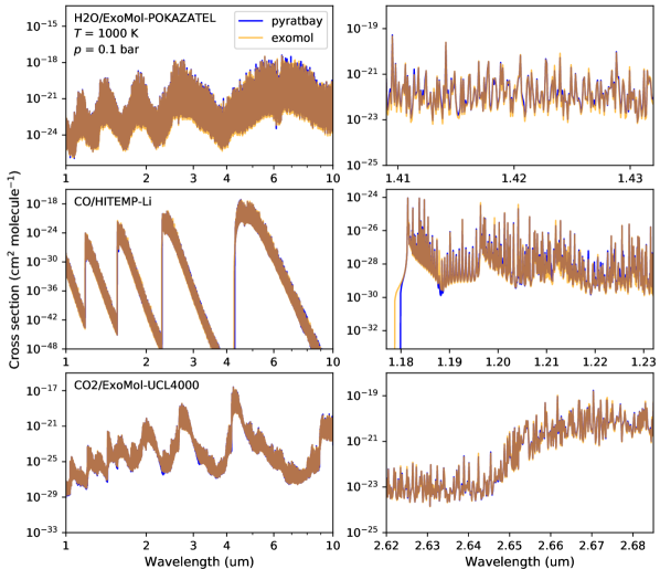
Figure 2: Line sampling comparison between Pyrat Bay (blue) and ExoMol (semi-transparent orange, Chubb et al., 2021). The top, middle, and bottom panels show H₂O, CO, and CO₂ line-by-line cross sections (respectively), sampled at a resolving power of ${\rm R}=10\,000$, evaluated at a temperature of $T=1000$ K and pressure of $p=0.1$ bar. The left panels show the cross sections over the 1–10 $\mu$m region, whereas the right panels show a selected narrow region for each molecule.

3.1 Cross Section Spectrum Benchmark

We benchmark the line-by-line cross-section sampling of Pyrat Bay by comparing its cross sections to the ExoMolOP database of Chubb et al. (2021). We selected three spectroscopically relevant species: the H₂O POKAZATEL line list of Polyansky et al. (2018), provided in ExoMol format; the CO line list of Li et al. (2015), provided in HITRAN format; and the CO₂ UCL4000 line list of Yurchenko et al. (2020), provided in ExoMol format. The only difference in the input line lists is that we pre-processed the H₂O database with the repack package, keeping only the strongest $\sim$9 million line transitions in the tested range (1–10 $\mu$m). Cross sections sampled from the repacked line lists show relative differences smaller than 1% by dex from the original line lists (submitted Cubillos, 2021)). We followed the methodology of Chubb et al. (2021) as closely as possible, considering the same isotopes for each of these molecules, sampling the spectrum at the same resolving power ${\rm R}=15\,000$ and wavelength locations, and assuming a solar atmospheric composition consisting primarily of $X_{\rm H2}=0.86$ and $X_{\rm He}=0.14$ (Asplund et al., 2009). Figure 2 shows an example of the resulting cross sections evaluated at 1000 K and 0.1 bar. In general, our results match well those of Chubb et al. (2021) at all temperatures and pressures. However, it is worth mentioning that the outputs can vary significantly depending on how the line profiles are modeled (e.g., line-wings cutoff), for which there is no clear prescription. We briefly discuss below how we computed the line profiles.

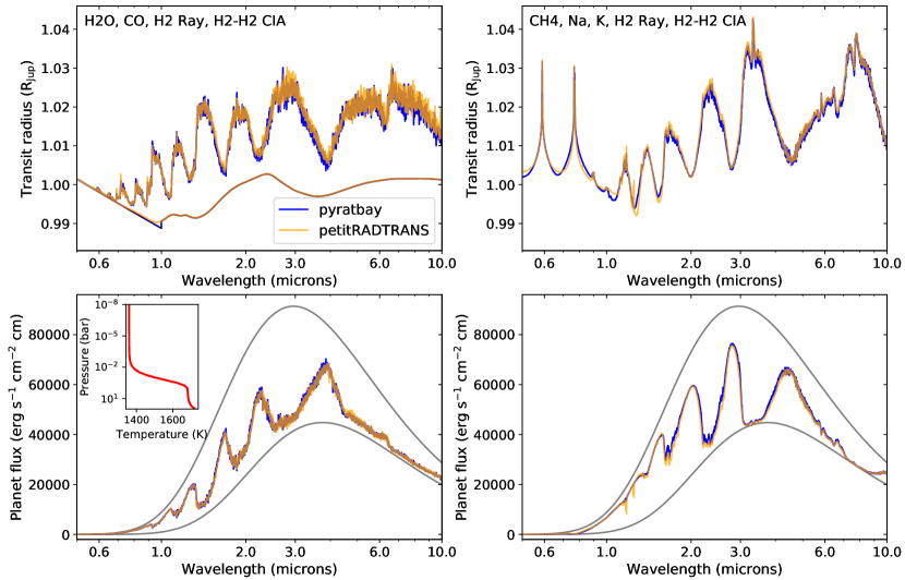
Figure 3: Transmission and emission spectra comparison between Pyrat Bay and petitRADTRANS. The solid blue and semi-transparent orange curves show the transmission (top panels) and emission spectra (bottom panels) computed by Pyrat Bay and petitRADTRANS, respectively. The models in the left panels consider H₂O and CO cross sections, whereas the models in the right panels consider CH₄, Na, and K cross sections. All models also consider H₂ Rayleigh and H₂–H₂ CIA cross sections. The smooth curves at the bottom of the top-left panel show spectra considering only Rayleigh and CIA cross section. The Pyrat Bay models have been smoothed from their original sampling rate (${\rm R}=10\,000$) to match that of petitRADTRANS (${\rm R}=1000$). The transmission models adopted an isothermal temperature profile at $T=1300$ K. The emission models adopted the temperature profile shown in the inset in the bottom left panel. The gray curves above and below the spectra show Planck emission models at the highest temperature (bottom layer) and lowest temperature (top layer) of the atmosphere, respectively. All scenarios show a good agreement between Pyrat Bay and petitRADTRANS.

The unknown extent of the line wings (Lévy et al., 1992) has one of the largest impacts on sampled cross sections (see, e.g., Grimm & Heng, 2015). Varying the line-wings cutoff can modify the sampled cross section by several orders of magnitude. Chubb et al. (2021) adopted a line-wing cutoff of 500 half-width at half maximum (HWHM) from the center of each line. For our sampling routine we adopted both a HWHM cutoff as well as a maximum fixed cutoff of 25 cm^-1. We found that cutoff values of 300 HWHM (for H₂O), 500 HWHM (CO), and 100 HWHM (CO₂) were sufficient to replicate the sampling of Chubb et al. (2021). Larger HWHM cutoff values did not change the results significantly, since the line profiles overlap due to the high density of lines and the fixed 25 cm^-1 cutoff caps the effect of much larger HWHM cutoff values. Note that the values adopted here are ad-hoc values that are typically used in the literature, they are not derived from theoretical first principles. For this reason, we deliberately designed the Pyrat Bay package to enable the users to compute the cross sections with custom cutoff values. One main difference between our methodology and Chubb et al. (2021) is collisional broadening calculation. Nonetheless, we do not see any major discrepancy between our cross sections and those of Chubb et al. (2021) despite these different approaches. Chubb et al. (2021) uses the HITRAN $\gamma$ and $n$ broadening parameters (Appendix of Rothman et al., 1998) to compute the collisional HWHM, applied for H₂ and He broadening (as opposed to self and air broadening). Pyrat Bay, instead, computes the collisional broadening based on the collision diameter of the atmospheric species (Goody & Yung, 1989).

3.2 Spectrum Forward-modeling Benchmark

We benchmark the radiative-transfer module of Pyrat Bay by comparing the output transmission and emission spectra to that of the open-source atmospheric-modeling framework petitRADTRANS (Mollière et al., 2019, commit f43559de). Both Pyrat Bay and petitRADTRANS adopt similar physical assumptions (e.g., LTE, plane-parallel atmosphere, hydrostatic equilibrium), however, the treatment of the cross section differs significantly. In particular, petitRADTRANS implements the $k$-distribution method under the correlated-$k$ approximation (Fu & Liou, 1992), whereas Pyrat Bay uses line sampling. To ensure that both codes use the same input atmospheric model, we generated the atmospheric profile with the petitRADTRANS code, which we then fed into Pyrat Bay. This limits the scope of the comparison to the radiative-transfer calculations. The atmosphere has 28 layers, extending from 100 to $10^{-5}$ bar. The composition is constant-with-altitude, dominated by H₂ and He, with volume mixing ratios of 0.85 and 0.149, respectively, and traces of H₂O (4$\times 10^{-4}$), CH₄ ($10^{-4}$), CO (3$\times 10^{-4}$), Na (3$\times 10^{-6}$), and K ($10^{-6}$). For transmission we used an isothermal profile at 1300 K. For emission we used the Guillot (2010) parameterization to generate a non-inverted profile where the temperature drops from $\sim$1700 K at the bottom of the atmosphere to $\sim$1350 K at the top of the atmosphere. The radius profile corresponds to a hydrostatic-equilibrium model of a $0.6{{M_{\rm Jup}}}$ planet with a radius of $1{{R_{\rm Jup}}}$ at 0.1 bar. We used the same cross section databases for both Pyrat Bay and petitRADTRANS: H₂–H₂ CIA (HITRAN), H₂O (POKAZATEL), CH₄ (YT10to10), and CO (HITRAN/Li). However, to speed up the calculation we pre-processed the H₂O and CH₄ line-list data with the repack code to preserve the 9 and 90 million stronger transitions, respectively, rather than the original 4 and 10 billion transitions in the 0.3–10 $\mu$m range. Figure 3 shows the resulting spectra for transmission (top panels) and emission (bottom panels), considering cross sections only for H₂ (top left panel), H₂O and CO (left panels) and for CH₄, Na, and K (right panels). We obtain consistent results between Pyrat Bay and petitRADTRANS in all scenarios. The difference in the Na and K lines is expected, since the two codes implement different alkali line-profile models (top right panel). petitRADTRANS assumed a Voigt profile, whereas Pyrat Bay assumed the power-law and exponential-decay model of Burrows et al. (2000). Other minor differences between the resulting spectra are well understood. In particular, at high pressures the CH₄ cross section of Pyrat Bay is stronger than that of the petitRADTRANS model, since petitRADTRANS applied an intensity cutoff for this molecule (top right panel). At low pressures the Pyrat Bay cross section is weaker than that of the petitRADTRANS models, since Pyrat Bay applied a line-wing cutoff proportional to the lines’ HWHM in addition to the fixed line-wing cutoff applied by both codes.

3.3 Retrieval Benchmark

We benchmark the atmospheric retrieval framework of Pyrat Bay by retrieving a set of synthetic spectra generated with the open-source package TauREx (Al-Refaie et al., 2019, version 3.0.3-beta), and comparing the posterior distributions to the input models. The benchmark sample consists of 12 planets for transmission and 12 planets for emission, selected from the Ariel target sample of Edwards et al. (2019). These planets span a broad range of physical properties in equilibrium temperature (450–2500 K), radius (1–20 $R_{\oplus}$), and mass (0.85 $M_{\oplus}$–9.0 $M$Jup). For the transmission models we adopted isothermal temperature profile models near the targets’ equilibrium temperatures. For the emission models we adopted Guillot (2010) temperature profiles, generating both inverted and non-inverted profiles. For each target, we used the open-source rate package (Cubillos et al., 2019) to estimate the atmospheric composition under thermochemical equilibrium. We sampled a variety of elemental compositions ranging from 0.5 to 30 times solar, and C/O ratios ranging form 0.05 to 0.9. We used these estimates as guidelines to set the composition of the synthetic models as constant-with-altitude volume mixing ratios. For the spectral calculations we considered CIA and Rayleigh cross sections from H₂, and line-sampling cross sections from H₂O, CH₄, CO, and CO₂. For the transmission models we also included an opaque gray cloud deck model. For both TauREx and Pyrat Bay we used the cross sections provided by TauREx. These cross sections are sampled at a constant resolving power of ${\rm R}=15\,000$, extending from 100 to 10-5 bar. For each target, we simulated Ariel-like observations (Tinetti et al., 2018), by integrating the synthetic spectra (0.45–8.0 $\mu$m) over the instrument bandpasses released for the Ariel retrieval challenge. We adopted a simple two-component noise model added in quadrature, where the first term is a constant noise floor level, and the second term is proportional to the square root of the stellar flux collected by each bandpass. We modeled the observed stellar fluxes as blackbody spectra according to the stellar effective temperatures, and scaled them according to their K-band apparent magnitudes. The Pyrat Bay retrieval adopts the same model parameterization as the input TauREx spectra. For transmission, the retrieval parameters are the isothermal temperature, the planetary radius at 100 bar, the volume mixing ratios of H₂O, CH₄, CO, and CO₂, and the pressure of the gray cloud deck. We assume uniform priors for all parameters. For emission, the retrieval parameters are the $\kappa^{\prime}$, $\gamma$, and $T_{\rm irr}$ parameters of the Guillot (2010) model (we kept $T_{\rm int}$ fixed at 100 K, as assumed by the TauREx models), the radius at 100 bar, and the volume mixing ratios of H₂O, CH₄, CO, and CO₂. We assume uniform priors for all parameters, except for the planetary radius. In the literature, the radius is generally assumed fixed for secondary-eclipse retrievals, even though this is not a known value a priori. We let this parameter free, and assume a Normal prior distribution according to the transit radius and 1$\sigma$ uncertainty of each planet. Table 3 summarizes the retrieval parameterization for these benchmark runs.

Table 3: Retrieval Benchmark Parameterization

Article	Transmission	Emission
Parameter	Priors∗	Priors∗
$T_{0}$ (K)	$\mathcal{U}(200,3000)$	$\cdots$
$\log_{10}(\kappa^{\prime})$	$\cdots$	$\mathcal{U}(-8.0,2.0)$
$\log_{10}(\gamma)$	$\cdots$	$\mathcal{U}(-5,5)$
$T_{\rm irr}$ (K)	$\cdots$	$\mathcal{U}(0,5000)$
$R_{\rm planet}$ (${R_{\rm Jup}}$)	$\mathcal{U}(0.5,30.0)$	$\mathcal{N}(R_{\rm p},\sigma_{R})$
$\log_{10}(X_{\rm H2O})$	$\mathcal{U}(-12,-1)$	$\mathcal{U}(-12,-1)$
$\log_{10}(X_{\rm CH4})$	$\mathcal{U}(-12,-1)$	$\mathcal{U}(-12,-1)$
$\log_{10}(X_{\rm CO})$	$\mathcal{U}(-12,-1)$	$\mathcal{U}(-12,-1)$
$\log_{10}(X_{\rm CO2})$	$\mathcal{U}(-12,-1)$	$\mathcal{U}(-12,-1)$
$\log_{10}(p_{\rm cloud}/{\rm bar})$	$\mathcal{U}(-4,2)$	$\cdots$

• ^∗ $\mathcal{U}(a,b)$ stands for a uniform distribution between $a$ and $b$. $\mathcal{N}(\mu,\sigma)$ stands for a normal distribution with mean $\mu$ and standard deviation $\sigma$.

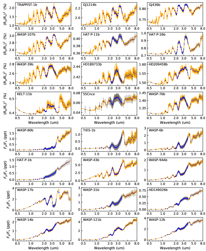
Figure 4: Synthetic Ariel sample of transmission (top panels) and emission (bottom panels) spectra. The blue markers with gray error bars show the TauREx synthetic models integrated over the Ariel observing bands and their 1$\sigma$ uncertainties, respectively. The orange curves show the Pyrat Bay retrieved best-fitting spectra.

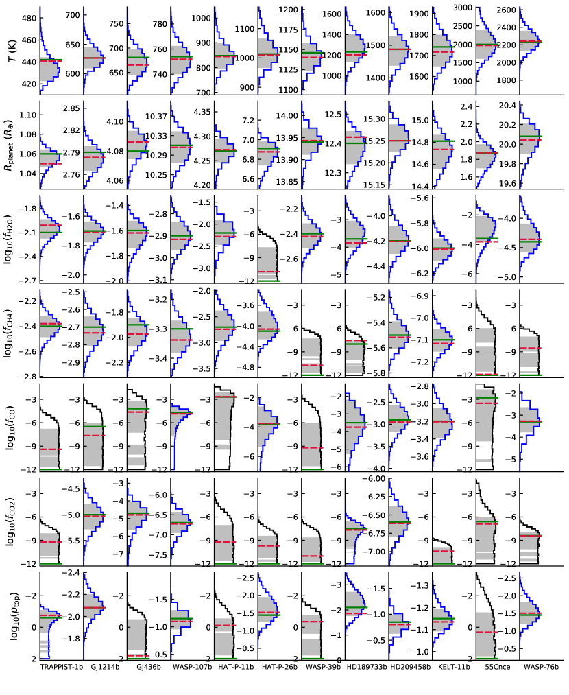
Figure 5: Retrieved marginal posterior distributions of the transmission-spectrum sample. Each column and row correspond to a target and retrieval parameter, respectively (see labels at the bottom and left of the figure). The gray shaded areas denote the 68% highest-posterior-density region (HPD, see Appendix in Cubillos et al., 2017) of each parameter (analogous to the 1$\sigma$ uncertainty for a Gaussian posterior). The solid green and dashed red lines denote the input and retrieved best-fitting values, respectively. The contour of the posterior distribution is colored black for the parameters with an upper limit constrain. For all constrained parameters, the input values are contained within the 68% HPD region, whereas for all upper limit constrains, the input values are contained within the 99% HPD region.

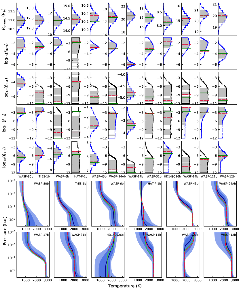
Figure 6: Retrieved posterior distributions of the emission-spectrum sample. Top: each column and row correspond to a target and retrieval parameter (except for the temperature-profile parameters), respectively (see labels at the bottom and left of the figure) Bottom: Temperature-profile posterior distribution. The dark and light blue shaded area denotes the span of the 68th and 95th percentiles of the temperature-profile posteriors, respectively. The green, red, and blue curves denote the input, best-fit, and median temperature profiles, respectively.

Figures 4, 5, and 6 show the retrieved spectra, transmission posterior distributions, and emission posterior distributions, respectively. All retrieved best-fitting spectra and posterior distributions are consistent with the input values from the TauREx models (within 1$\sigma$). The precision of the posterior distributions are consistent with expectations based on the signal-to-noise ratio of the input spectra. Note that in several cases it is not possible to constrain all parameters. Often the most spectroscopically active and abundant species (e.g., H₂O) cover the spectral features of other species (e.g., CO or CO₂). It is thus expected to find weakly constrained posteriors or upper limits for certain molecules. Overall, the abundance constraints are stronger for the transit simulations than for the eclipse simulations, which we can explain in two ways. First, the transit simulations have larger signal-to-noise ratios than the eclipse simulations, since they generally have brighter stars and show stronger spectral modulations (on the order of percents rather than parts per thousand). Second, the eclipse retrievals use a more complex temperature profile than the transit retrievals. Since the emission features arise from the variation of the thermal structure (the location and magnitude of the thermal gradient), the parameters for the abundances and thermal structure correlate to generate a degenerate family of solutions. Figure 6 shows evidence of this behavior. In general, larger temperature gradients lead to stronger features, which are easier to constrain. Note, for example, that the nearly isothermal atmosphere of the HAT-P-1b simulation places the weakest abundance constraints, whereas the WASP-17b simulation places the strongest abundance constraints.

3.4 HD 209458 b Benchmark

As a final benchmark test, we applied the Pyrat Bay atmospheric retrieval to real transmission observations and compare our results to that of previous studies. We chose HD 209458 b, an inflated hot Jupiter orbiting one of the brightest and nearest stars known to host an exoplanet (Charbonneau et al., 2000; Henry et al., 2000; Mazeh et al., 2000). The extraordinarily favorable observing conditions of this planet have made HD 209458 b the poster child for most exoplanet observing techniques, including atmospheric retrievals. Here we considered the space-based transmission spectrum of HD 209458 b reported by Sing et al. (2016), obtained from HST (0.29–1.0 $\mu$m with STIS, 1.1–1.7 $\mu$m with WFC3) and Spitzer observations (3.6 and 4.5 $\mu$m with IRAC). We compared our results with those of the poseidon (MacDonald & Madhusudhan, 2017) and Aura code (Pinhas et al., 2019), henceforth named MM2017 and P2019, respectively. We chose these analyses since we can re-analyze the data in a similar fashion to MM2017 and P2019, and therefore, make a more direct comparison of the retrieval results. We configured our model setup and parameterization to follow that of MM2017 and P2019, deviating only when we could not replicate their approach (which we will point out in the text). Thus, we adopted the same system parameters (Torres et al., 2008), transmission observations, model parameterization, and priors used by MM2017 and P2019. Our atmospheric model consisted of 41 pressure layers extending from $10^{-6}$ bar to 100 bar, using the temperature profile parameterization of Madhusudhan & Seager (2009), a primary-atmosphere composition with a solar H₂/He abundance ratio, and an altitude profile in hydrostatic equilibrium. We adopted constant-with-altitude abundance profiles for all species. The radiative-transfer model considered line-by-line cross sections from H₂O (Polyansky et al., 2018), CH₄ (Yurchenko & Tennyson, 2014), HCN (Harris et al., 2006, 2008), NH₃ (Yurchenko, 2015; Coles et al., 2019), CO (Li et al., 2015), and CO₂ (Rothman et al., 2010). Prior to the MCMC runs, we applied the repack algorithm (Cubillos, 2017) to the ExoMol line lists to extract only the dominant transitions. Then, we sampled the line-by-line cross sections into $R=15\,000$ cross-section tables evaluated at the pressures of the atmospheric model and over a temperature array evenly spaced from 100 K to 3000 K with a step of 100 K. The model also included collision-induced absorption for H₂–H₂ pairs (Borysow et al., 2001; Borysow, 2002) and H₂–He pairs (Borysow et al., 1988, 1989; Borysow & Frommhold, 1989); Rayleigh-scattering cross section for H₂ (Dalgarno & Williams, 1962) and for an unknown haze particulate (Lecavelier Des Etangs et al., 2008); Na and K resonance line cross sections; and a gray cloud deck parameterized by the cloud top pressure ($p_{\rm top}$). Lastly, we included the patchy cloud/haze fraction parameter $f_{\rm patchy}$. For MM2017, we re-analyzed their ‘fixed-fraction’ retrieval (Section 4.1 of MM2017). This analysis only considers the HST observations, neglects the contribution from CO and CO₂, and fixes the patchy cloud/haze fraction parameter at $f_{\rm patchy}=0.47$. The main difference between our and their setup is that we let $X_{\rm K}$ to be a free parameter, whereas MM2017 kept the ratio $X_{\rm K}/X_{\rm Na}$ fixed according to the solar volume-mixing ratios. Another difference is that for the hydrostatic equilibrium solution we fixed a reference pressure point ($p_{\rm ref}$) and let its corresponding altitude free ($R_{\rm planet}$); whereas MM2017 and P2019 fixed a reference altitude point and retrieved the logarithm of its corresponding pressure. Welbanks & Madhusudhan (2019) showed that the choice of $p_{\rm ref}$ or $R_{\rm planet}$ as free parameter does not impact the retrieval results. To ease the comparison, for the reference pressure we chose the best-fitting $p_{\rm ref}$ of MM2017 and P2019 (thus, ideally, our retrieval radius should match their reference altitude). Table 4 summarizes our retrieval parameterization for the MM2017 and P2019 re-analyses.

Table 4: HD 209458b Retrieval Parameters Summary

Reference	MM2017	P2019
Parameter	Priors∗	Priors∗
$\log_{10}(p_{1}/{\rm bar})$	$\mathcal{U}(-6,2)$	$\mathcal{U}(-6,2)$
$\log_{10}(p_{2}/{\rm bar})$	$\mathcal{U}(-6,2)$	$\mathcal{U}(-6,2)$
$\log_{10}(p_{3}/{\rm bar})$	$\mathcal{U}(-2,2)$ and $p_{3}>p_{1}$	$\mathcal{U}(-2,2)$ and $p_{3}>p_{1}$
$a_{1}$ (K-0.5)	$\mathcal{U}(0.02,1.0)$	$\mathcal{U}(0.02,1.0)$
$a_{2}$ (K-0.5)	$\mathcal{U}(0.02,1.0)$	$\mathcal{U}(0.02,1.0)$
$T_{0}$ (K)	$\mathcal{U}(800,1600)$	$\mathcal{U}(800,1650)$
$R_{\rm planet}$ ($R_{\rm Jup}$)	$\mathcal{U}(0.5,2.0)$	$\mathcal{U}(0.5,2.0)$
$\log_{10}(X_{\rm Na})$	$\mathcal{U}(-10,-2)$	$\mathcal{U}(-12,-2)$
$\log_{10}(X_{\rm K})$	$\mathcal{U}(-10,-2)$	$\mathcal{U}(-12,-2)$
$\log_{10}(X_{\rm H2O})$	$\mathcal{U}(-10,-2)$	$\mathcal{U}(-12,-2)$
$\log_{10}(X_{\rm CH4})$	$\mathcal{U}(-10,-2)$	$\mathcal{U}(-12,-2)$
$\log_{10}(X_{\rm NH3})$	$\mathcal{U}(-10,-2)$	$\mathcal{U}(-12,-2)$
$\log_{10}(X_{\rm HCN})$	$\mathcal{U}(-10,-2)$	$\mathcal{U}(-12,-2)$
$\log_{10}(X_{\rm CO})$	Fixed $(-12)$	$\mathcal{U}(-12,-2)$
$\log_{10}(X_{\rm CO2})$	Fixed $(-12)$	$\mathcal{U}(-12,-2)$
$\log_{10}(P_{\rm top}/{\rm bar})$	$\mathcal{U}(-6,2)$	$\mathcal{U}(-6,2)$
$\log_{10}(f_{\rm ray}$)	$\mathcal{U}(-4,8)$	$\mathcal{U}(-4,8)$
$\alpha_{\rm ray}$	$\mathcal{U}(-20,2)$	$\mathcal{U}(-20,2)$
$f_{\rm patchy}$	Fixed $(0.47)$	$\mathcal{U}(0,1)$

• ^∗ $\mathcal{U}(a,b)$ stands for a uniform distribution between $a$ and $b$.

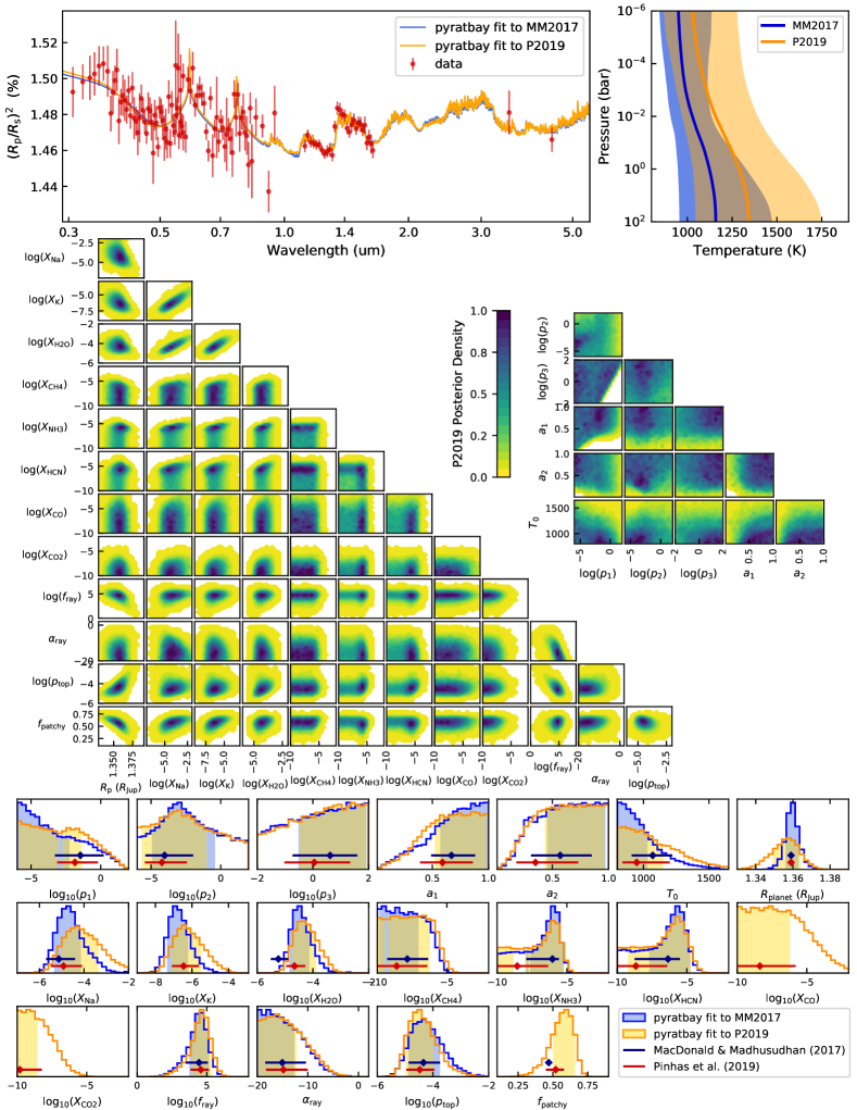
Figure 7: Pyrat Bay retrieval of the transmission spectra of HD 209458 b. In all panels, the blue- and orange-themed curves correspond to our re-analysis of the MM2017 and P2019 analyses, respectively. Top left: HD 209458 b observed spectra (red markers with error bars) and best-fitting model to the MM2017 and P2019 datasets. Top right: posterior temperature profiles. The solid curves and shaded areas mark the median and the 68% central credible intervals of the posterior distributions, respectively. Middle: pair-wise posterior distributions for the P2019 Pyrat Bay re-analysis (our re-analysis of MM2017 followed similar patterns). Bottom: marginal posterior distributions. The shaded areas denote the 68% highest-posterior-density credible intervals. The blue and red markers with error bars denote median and 68% central credible intervals obtained by MM2017 and P2019, respectively.

Figure 7 shows our retrieval results (spectra, temperature profiles, pair-wise posteriors, and marginal posteriors) and compares our marginal posteriors to those of MM2017 and P2019. We found a good agreement between our retrieval results and those of MM2017 and P2019. Our best-fitting spectra match well the observations ($\chi^{2}_{\rm red}=\sim 1.5$), and resemble the models retrieved by MM2017 and P2019. Our temperature profiles show a similar (non-inverted) behavior to that of MM2017 and P2019. Although our profiles are consistently $\sim$100–200 K colder than theirs at the pressures probed by the observations ($p\lesssim 0.1$ bar), our temperature-profile credible intervals overlap with those of MM2017 and P2019. For most parameters, our pair-wise posterior distributions show the same trends and correlations as those of MM2017 and P2019; for example, compare our pair-wise posteriors for the P2019 re-analysis from Fig. 7 (our re-analysis of MM2017 followed similar patterns) to Fig. 9 of MM2017. The major discrepancy lies in the $p_{2}$-vs.-$p_{1}$ panel, the posterior distribution of MM2017 shows an abrupt edge at $p_{2}=p_{1}$, suggesting that their retrieval imposed a $p_{2}<p_{1}$ condition (i.e., requiring a non-inverted profile). We allowed for any combination of $p_{1}$ and $p_{2}$ values within their prior ranges. Our marginal posterior distributions match well those of MM2017 and P2019 (significant overlap of the credible intervals), except for some temperature-profile parameters, which is not surprising considering the potential discrepancy noted above. As in the previous studies by MM2017 and P2019, our retrievals constrain the abundances of H₂O, Na, K, and a combination of HCN or NH₃. For CO, CO₂, and CH₄, our retrievals place upper limits to their abundances. Our retrievals favor a cloud top located at ${p_{\rm top}}\approx 5\times 10^{-5}$ bar with a partially cloudy atmosphere for the P2019 dataset ($f_{\rm patchy}\sim 0.5$). Lastly, we also recover a super-enhanced and super-Rayleigh haze absorption ($f_{\rm ray}\approx 10^{4}$–$10^{5}$, $\alpha_{\rm ray}\approx-15$). Ohno & Kawashima (2020) propose that such super-Rayleigh slopes can arise from photochemical hazes present in an atmosphere exhibiting with strong vertical mixing.

Table 5: Physical Properties and Datasets of our WFC3 Sample.

Planet	$R_{\rm p}$	$M_{\rm p}$	${T_{\rm eq}^{*}}$	$R_{\rm s}$	$M_{\rm s}$	$a$	$T_{\rm eff}$	System-parameter	Transmission-data	Observing Proposal
	$R$Jup	$M$Jup	K	$R_{\odot}$	$M_{\odot}$	AU	K	References	References	PI (ID)
GJ 436b	0.366	0.08	630	0.455	0.556	0.0308	3416	Lanotte et al. (2014)	Tsiaras et al. (2018)	Stevenson (13338)
HAT-P-3b	0.899	0.596	1160	0.833	0.93	0.0388	5185	Torres et al. (2008)	Tsiaras et al. (2018)	Deming (14260)
HAT-P-17b	1.01	0.534	780	0.838	0.857	0.0882	5246	Howard et al. (2012)	Tsiaras et al. (2018)	Huitson (12956)
HAT-P-18b	0.947	0.196	840	0.717	0.77	0.0559	4870	Esposito et al. (2014)	Tsiaras et al. (2018)	Deming (14260)
HAT-P-32b	1.790	0.86	1780	1.22	1.16	0.034	6210	Hartman et al. (2011)	Damiano et al. (2017)	Deming (14260)
HAT-P-32b	1.79	0.86	1780	1.22	1.16	0.034	6210	Hartman et al. (2011)	Tsiaras et al. (2018)	Deming (14260)
HAT-P-38b	0.82	0.267	1080	0.92	0.89	0.052	5330	Sato et al. (2012)	Bruno et al. (2018)	Deming (14260)
HAT-P-38b	0.82	0.267	1080	0.92	0.89	0.052	5330	Sato et al. (2012)	Tsiaras et al. (2018)	Deming (14260)
HAT-P-41b	1.685	0.8	1940	1.683	1.418	0.0426	6390	Hartman et al. (2012)	Tsiaras et al. (2018)	Deming (14260)
HD 149026b	0.654	0.359	1670	1.368	1.29	0.0431	6160	Torres et al. (2008)	Tsiaras et al. (2018)	Deming (14260)
K2-18b	0.242	0.027	290	0.469	0.495	0.1591	3503	Cloutier et al. (2019)	Benneke et al. (2019)	Benneke (13665)
K2-18b	0.203	0.025	290	0.411	0.359	0.1429	3457	Benneke et al. (2017)	Tsiaras et al. (2019)	Benneke (13665)
WASP-29b	0.792	0.244	970	0.808	0.825	0.0457	4800	Hellier et al. (2010)	Tsiaras et al. (2018)	Deming (14260)
WASP-43b	1.04	2.03	1460	0.67	0.72	0.015	4520	Gillon et al. (2012)	Stevenson et al. (2017)	Bean (13467)
WASP-43b	0.93	1.78	1440	0.67	0.71	0.0142	4400	Hellier et al. (2011)	Tsiaras et al. (2018)	Bean (13467)
WASP-63b	1.43	0.38	1540	1.88	1.32	0.057	5550	Hellier et al. (2012)	Kilpatrick et al. (2018)	Stevenson (14642)
WASP-63b	1.43	0.38	1540	1.88	1.32	0.057	5550	Hellier et al. (2012)	Tsiaras et al. (2018)	Stevenson (14642)
WASP-67b	1.40	0.42	1040	0.87	0.87	0.052	5200	Hellier et al. (2012)	Bruno et al. (2018)	Deming (14260)
WASP-67b	1.40	0.42	1040	0.87	0.87	0.052	5200	Hellier et al. (2012)	Tsiaras et al. (2018)	Deming (14260)
WASP-69b	1.057	0.26	960	0.813	0.826	0.0452	4715	Anderson et al. (2014)	Tsiaras et al. (2018)	Deming (14260)
WASP-74b	1.56	0.95	1920	1.64	1.48	0.037	5970	Hellier et al. (2015)	Tsiaras et al. (2018)	Sing (14767)
WASP-80b	0.999	0.538	820	0.586	0.577	0.0344	4143	Triaud et al. (2015)	Tsiaras et al. (2018)	Deming (14260)
WASP-101b	1.41	0.50	1560	1.29	1.34	0.051	6400	Hellier et al. (2014)	Wakeford et al. (2017b)	Sing (14767)
WASP-101b	1.41	0.50	1560	1.29	1.34	0.051	6400	Hellier et al. (2014)	Tsiaras et al. (2018)	Sing (14767)
WASP-103b	1.528	1.49	2510	1.436	1.22	0.0198	6110	Gillon et al. (2014)	Kreidberg et al. (2018a)	Kreidberg (14050)
XO-1b	1.206	0.918	1210	0.934	1.03	0.0493	5750	Torres et al. (2008)	Tsiaras et al. (2018)	Deming (12181)

• ^∗ Assuming zero albedo and efficient energy redistribution (i.e., reemission over $4\pi$ radians).

4 A Systematic Atmospheric Retrieval of Exoplanet Transmission Observations

Here, we begin a systematic analysis of the existing space-based exoplanet transmission spectra. The goals of this study are to produce a large sample of targets analyzed under a standard set of retrievals and present an independent reanalysis of published results. The sample includes all targets with published transit spectra with sufficient wavelength coverage and resolution to resolve atmospheric spectral features, discarding targets with only broadband photometric observations. By applying a standardized retrieval analysis across the sample, we can compare the results of the different retrievals for a given target, as well as the results between targets.

4.1 Target Sample

In this article, we analyze the targets without observations at wavelengths shorter than 1 $\mu$m (as of early 2020). This sample includes 26 datasets of 19 different systems observed with the Hubble Wide Field Camera 3 (WFC3), using the G141 grism (1.1 to 1.7 $\mu$m). Among them, three datasets (K2-18b, WASP-43b, and WASP-103b) also include observations from the Spitzer Infrared Array Camera (IRAC), using the 3.6 and 4.5 $\mu$m photometric filters. Future articles will present the analysis of the targets with shorter-wavelength observations (namely, from the Hubble STIS and WFC3/G104 data). Table 5 lists the datasets considered in this sample and the main properties of their systems. To enable a more direct comparison between our results and those published, for each dataset we adopted the same system parameters as those assumed in the original article. We focus our analysis on characterizing the H₂O absorption signature, since this molecule is expected to dominate the spectral range probed by the HST WFC3/G141 grism. We pay particular attention to the strong degeneracies between the H₂O abundance, cloud coverage, and atmospheric mean molecular mass, which can lead to similar transmission absorption spectra, especially for observations over a narrow wavelength range such as this one (see, e.g., Griffith, 2014; Madhusudhan et al., 2014; Line & Parmentier, 2016; Fu et al., 2017). To determine in a statistically robust manner whether the data can distinguish between such scenarios, for each dataset we run a set of retrievals including or excluding clouds, and with or without a parameter that varies the atmospheric mean molecular mass. We compare the results using the Bayesian Information Criterion (BIC, Liddle, 2007). To assess the significance of the model comparison, we adopt the Raftery (1995) rule of thumb, ranking the evidence as weak (for $\Delta$BIC values within 0–2), positive (2–6), strong (6–10), and very strong (values greater than 10), where $\Delta$BIC is the difference in BIC between a given model and the lowest-BIC model for the dataset.

4.2 Retrieval Setup

To yield a uniformly analyzed sample, we apply the Pyrat Bay retrieval under the same set of assumptions for each dataset, where we set free parameters for the atmospheric temperature, composition, cloud coverage, and altitude profile models. For specific cases we perform additional retrieval tests, for example, search for additional molecules when there is Spitzer data or when there is prior evidence for them. We retrieve the atmospheric abundances as constant-with-altitude volume-mixing-ratio profiles, setting a lower boundary at $10^{-12}$, at which their spectral features become negligible. For the Jupiter-type planets ($M_{\rm p}\gtrsim 0.3{M_{\rm Jup}}$), we limit the sum of the mixing ratios of the metals to be less than 0.2 (i.e., the MCMC rejects samples where $X_{\rm H2}+X_{\rm He}<0.8$, see Eq. (25)), which roughly corresponds to a maximum metallicity of $\sim$250$\times$ solar (thus, ensuring H₂/He-dominated atmospheres). For the sub-Saturn mass planets ($M_{\rm p}\lesssim 0.3{M_{\rm Jup}}$) we relax the limit the sum of the metal mixing ratios to be less than 0.9. As in previous studies (e.g., Line et al., 2013; Tsiaras et al., 2018; Welbanks et al., 2019), these metallicity upper boundaries are rough estimates based on the bulk properties of the planets. More precise estimates could be obtained on a case-by-case basis from interior-structure and evolution models, constrained by the planet’s mass, radius, and age (see, e.g., Thorngren et al., 2016; Kreidberg et al., 2018b), but such analysis lies beyond the scope of this work. For HAT-P-38b and K2-18b we set the temperature upper limit at a stricter $T_{\rm eq}^{\rm max}+3\sigma_{T}$, since the posterior distributions were returning temperatures far in excess above their maximum estimated equilibrium temperatures ($T_{\rm eq}^{\rm max}$, for zero albedo and no day–night energy redistribution). These upper limits are 1500 K and 390 K for HAT-P-38b and K2-18b, respectively. We consider uniform priors in log scale for the mixing ratios. For all datasets we retrieve the H₂O abundance. For the datasets that include Spitzer observations, we also retrieve the CH₄ abundance (expected to have features at 3.6 $\mu$m) and the CO and CO₂ abundances (expected to have features at 4.5 $\mu$m). Lastly, for WASP-63b we also retrieve the HCN abundance, given the prior evidence for its detection (Kilpatrick et al., 2018). We retrieve the temperature profile adopting the isothermal model. This is an appropriate choice for these datasets given the weak sensitivity of transmission spectra to temperature gradients and the narrow pressure range probed by these observations (Barstow et al., 2013; Rocchetto et al., 2016). We let the temperature vary between 100 and 3000 K (the range allowed by the cross sections), adopting a uniform prior. We retrieve the altitude profile adopting Eq. (6) to compute hydrostatic equilibrium. To solve this equation we retrieve the planetary radius $R_{\rm planet}$ at a reference pressure level of $p_{0}=0.1$ bar. We let the planetary radius vary within 0.1 and 4 $R$Jup (though none of the retrievals reached these boundaries), adopting a uniform prior. Additionally, we retrieve the abundance of N₂ (without considering its absorption cross section), which works as a proxy to vary the mean molecular mass $\mu$ independently of the other free-abundance species that affect the atmospheric cross section. In practice, we monitor the metal mass fraction relative to the sun:

$$[Z/X]=\log_{10}(Z/X)-\log_{10}(Z/X)_{\odot},$$ (26)

where $X$ and $Z$ are the hydrogen and metal mass fractions, respectively. We adopt the solar mass fraction values from Asplund et al. (2009): $X_{\odot}=0.7381$ and $Z_{\odot}=0.0134$. Recalling that $X+Y+Z=1$ (see, e.g., Carroll & Ostlie, 1996), with $Y$ the helium mass fraction, we compute the metal mass fraction from $Z=1-X-Y$. To compute $X$ and $Y$ we need to account for the volume mixing ratios $X_{i}$ of all atmospheric species containing hydrogen and helium (respectively), weighted by their stoichiometric coefficients, i.e.: $X=(2X_{\rm H2}+2X_{\rm H2O}+X_{\rm HCN}+4X_{\rm CH4})\,m_{\rm H}/\mu$ and $Y=X_{\rm He}\,m_{\rm He}/\mu$. We prefer to show the metal mass fraction (Eq. (26)) instead of the mean molecular mass because it offers a metric much more sensitive to the composition of the atmosphere, since it can trace the metal content across several orders of magnitude. Instead, the mean molecular mass converges to $\mu\approx 2.3$ for all solar/sub-solar metallicities. Finally, we consider the gray cloud deck model. We retrieve the pressure at the top of the cloud deck ($p_{\rm top}$), which can vary within 100 and $10^{-6}$ bar, adopting a uniform prior in log scale. Table 6 summarizes the retrieval parameterization for the WFC3 sample.

Table 6: Retrieval Parameters Summary

Parameter	Priors∗
$T$ (K)	$\mathcal{U}(100,3000)$
$R_{\rm planet}$ ($R_{\rm Jup}$)	$\mathcal{U}(0.1,4.0)$
$\log_{10}(X_{\rm H2O})$	$\mathcal{U}(-12,0)$
$\log_{10}(X_{\rm CO})^{\dagger}$	$\mathcal{U}(-12,0)$
$\log_{10}(X_{\rm CO2})^{\dagger}$	$\mathcal{U}(-12,0)$
$\log_{10}(X_{\rm CH4})^{\dagger}$	$\mathcal{U}(-12,0)$
$\log_{10}(X_{\rm HCN})^{\ddagger}$	$\mathcal{U}(-12,0)$
$\log_{10}(X_{\rm N2})^{\S}$	$\mathcal{U}(-12,0)$
$\log_{10}({p_{\rm top}}/{\rm bar})$	$\mathcal{U}(-6,2)$
	$X_{\rm H2}+X_{\rm He}>0.8^{\P}$

• ^∗ $\mathcal{U}(a,b)$ stands for a uniform distribution between $a$ and $b$.

• ^† Only considered for datasets with Spitzer observations.

• ^‡ Only considered for WASP-63b datasets.

• ^§ Used as proxy to enhance the atmospheric metal mass fraction.

• ^¶ Only imposed for Saturn/Jupiter-mass planets ($M_{\rm p}\gtrsim 0.2{M_{\rm Jup}}$).

For the molecular line-by-line cross sections we consider the ExoMol databases for H₂O (Polyansky et al., 2018), CH₄ (Yurchenko & Tennyson, 2014), and HCN (Harris et al., 2006, 2008); and the HITEMP databases for CO (Li et al., 2015) and CO₂ (Rothman et al., 2010). Before computing the cross sections, we apply the repack compression to the large ExoMol line lists to reduce the number of transitions to compute. We then sample the line-by-line cross sections at a constant resolving power of ${\rm R}=15\,000$ between 1.0 and 5.5 $\mu$m. We sample the cross-section spectra into a grid of 41 pressure layers between 100 and $10^{-8}$ bar and 30 temperature samples between 100 and 3000 K. During the retrieval, the MCMC sampler interpolates in temperature from this grid. Additionally, the atmospheric model includes Rayleigh scattering cross section for H₂ and CIA cross section for H₂–H₂ and H₂–He (Borysow et al., 1988, 1989; Borysow et al., 2001; Borysow, 2002; Borysow & Frommhold, 1989). We sample the posterior parameter space with the Snooker DEMC algorithm (ter Braak & Vrugt, 2008) implemented via the mc3 package. We obtain between 1 and 6 million samples, distributed into 24 parallel chains (discarding the first 10 000 iterations from each chain). To check for convergence we apply the Gelman-Rubin statistics (Gelman & Rubin, 1992), checking that the potential scale reduction factor approaches $\sim$1.01 or lower for each free parameter.

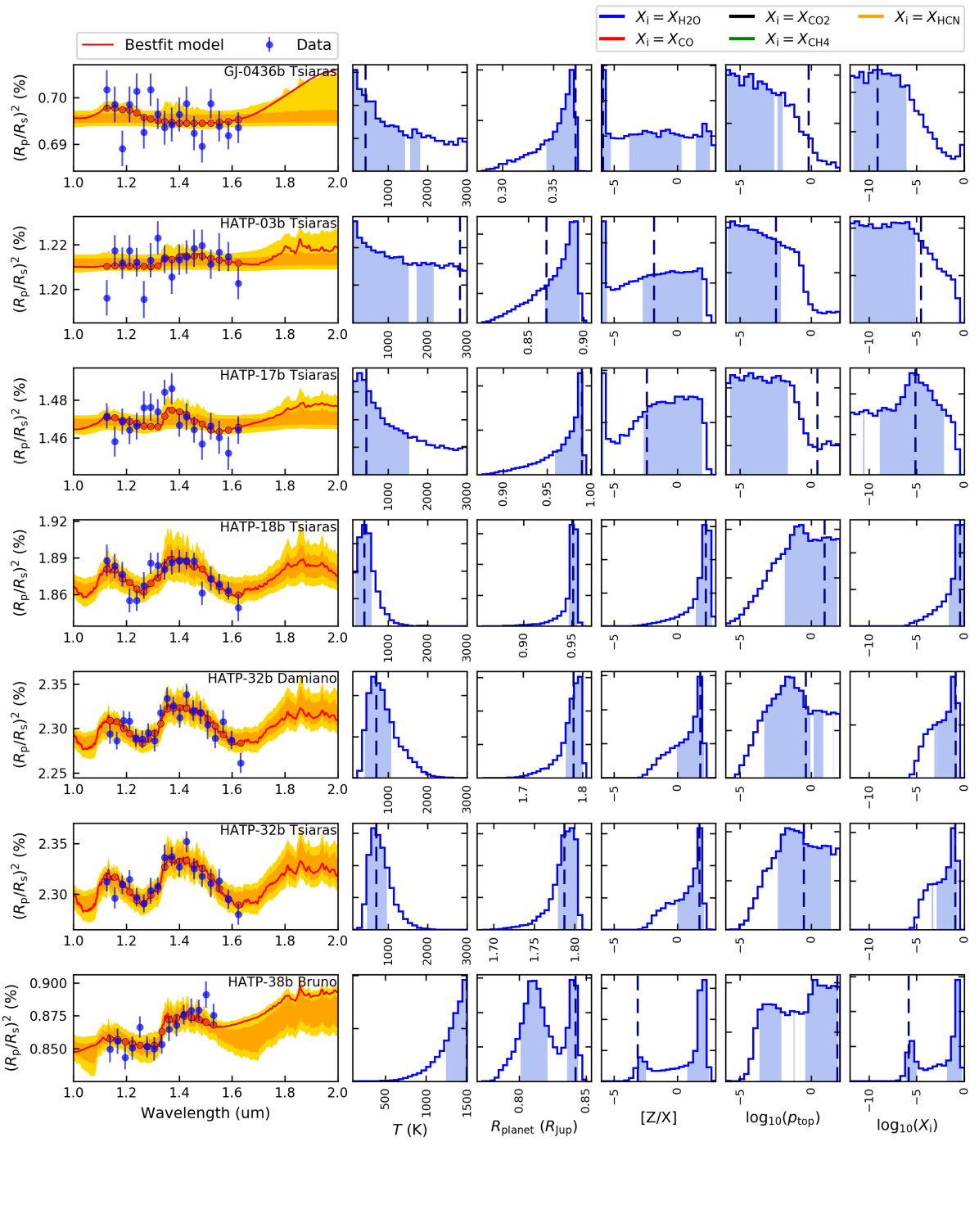
Figure 8: Pyrat Bay retrieval of the WFC3 transmission sample. Left panels: observed transmission spectra with 1$\sigma$ uncertainties (blue dots with error bars) and retrieved best-fitting models (red curves). The orange and yellow contours denote the span of the 68th and 95th percentile of the MCMC posterior distribution, respectively. The label at the top right corner of each panel indicates the name of the dataset. Following panels: retrieved marginal posterior histograms of the corresponding datasets shown in the left panels. The shaded areas denote the 68% HPD credible regions of the distributions. The panels on the far right might show the posterior for multiple species, color coded according to the labels at the top of the figure. The dashed vertical lines denote the best-fitting values for each parameter.

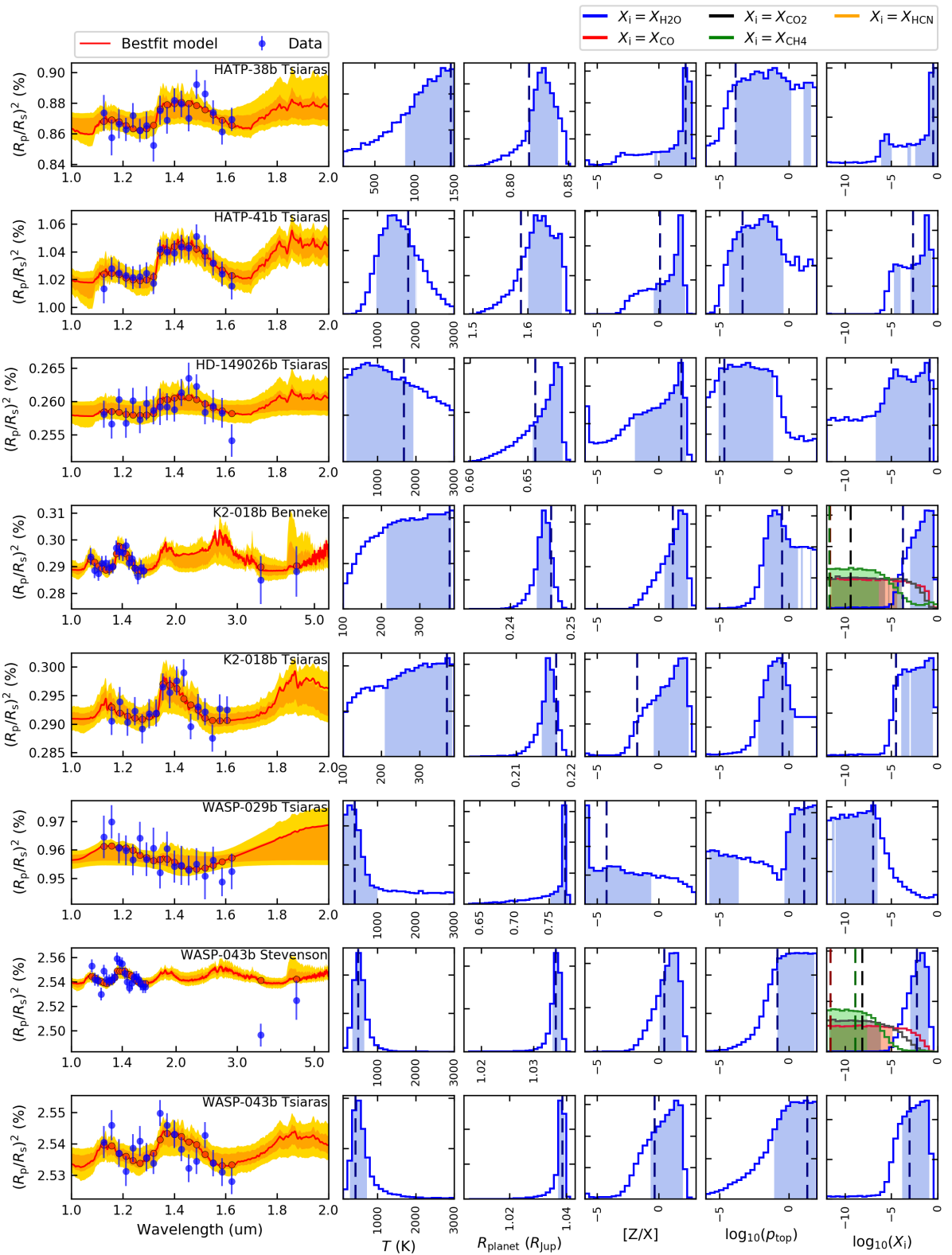
Figure 9: Pyrat Bay retrieval of the WFC3 transmission sample (continuation). See caption in Figure 8.

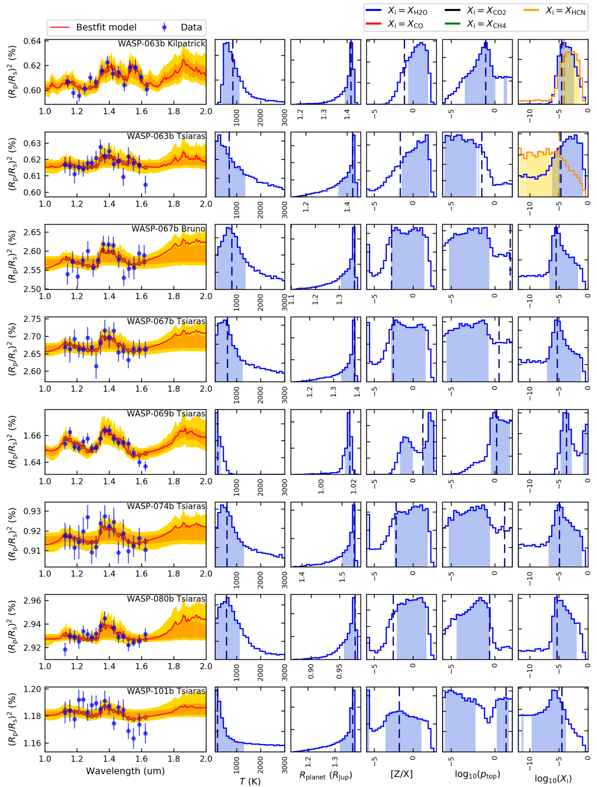
Figure 10: Pyrat Bay retrieval of the WFC3 transmission sample (continuation). See caption in Figure 8.

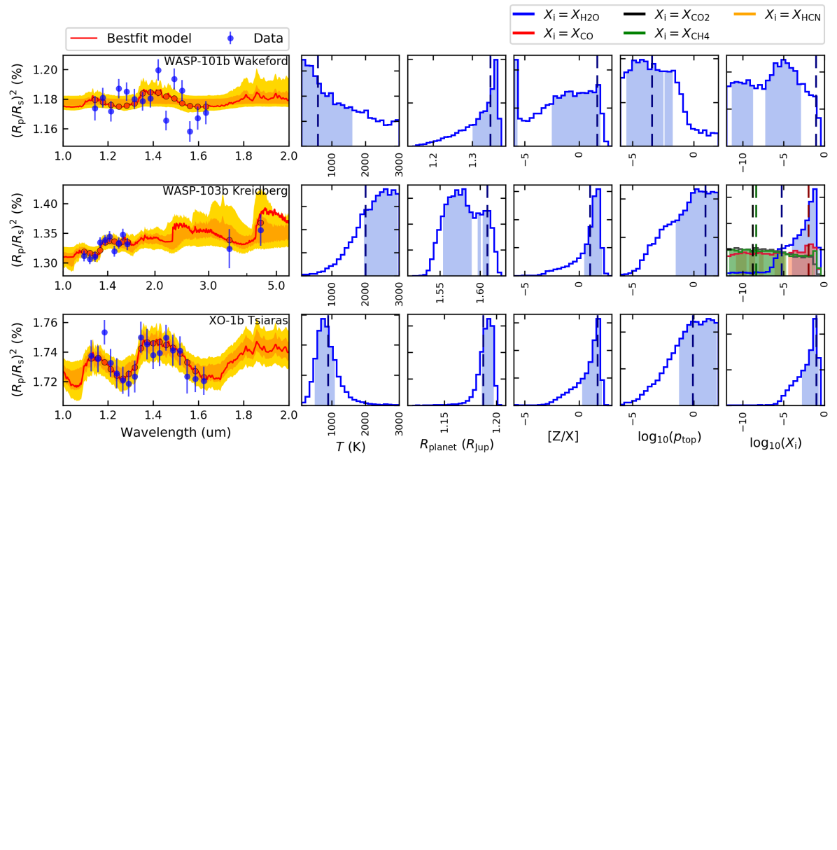
Figure 11: Pyrat Bay retrieval of the WFC3 transmission sample (continuation). See caption in Figure 8.

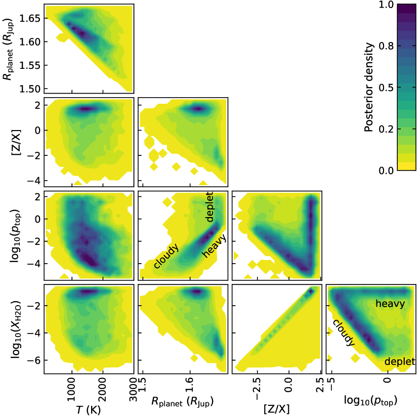
Figure 12: Pyrat Bay pair-wise posterior distributions of the HAT-P-41b/Tsiaras WFC3 transmission spectrum. This figure exemplifies a typical correlation between parameters found in the overall sample analysis. We selected two panels to label the different solution modes where the atmospheric models are preferentially cloudy (‘cloudy’), high in metal mass fractions (‘heavy’), and depleted in H₂O abundance (‘deplet’). The posterior distribution transitions smoothly from one region to another.

4.3 Results

The datasets in this sample show a wide variety of spectral features, ranging from featureless and noisy spectra to well defined absorption bands that are consistent with the H₂O absorption signature. Figures 8–11 show the retrieved spectra and marginal posterior distributions for our sample. In these runs we retrieve the cloud top pressure, the metal mass fraction [Z/X] (via the N₂ free abundance), and the CH₄, CO, CO₂, and HCN abundances when applicable. Tables 8–11 in the appendix show the model comparison statistics for each dataset. Based on the BIC model comparison, we found that 15 out of the 26 datasets are better explained by a H₂O absorption feature rather than a flat transmission spectrum; however, none of these datasets yield a $\Delta$BIC significant enough to distinguish between a cloudy or a high metal-mass-fraction scenario (i.e., $|{\rm BIC}_{\rm M1}-{\rm BIC}_{\rm M2}|<2$). The retrieved model spectra reproduce well the observations for most datasets, finding ${\chi^{2}_{\rm red}}$ values close to one (with the exception of WASP-43b, WASP-69b, and WASP-101b). However, the posterior distributions reveal strong correlations between many of the free parameters. These correlations lead to broad, multi-modal, or unconstrained marginal posteriors. Figure 12 shows a typical pair-wise posterior distribution, obtained from the HAT-P-41b/Tsiaras Pyrat Bay retrieval. We found that the temperature correlates strongly with the planets’ reference altitude at 0.1 bar. The temperature also often shows non-linear correlation with the cloud top pressure. The posterior multimodality is more clearly seen in the $p_{\rm top}$, [Z/X], and $X_{\rm H2O}$ correlation panels (see labeled regions in Fig. 12). The two main solution modes are a cloudy mode, characterized by a strong $p_{\rm top}$–$X_{\rm H2O}$ correlation, and a heavy atmosphere, characterized by a high metal mass fraction (driven mainly by the high $X_{\rm H2O}$), where clouds become irrelevant. We also often see a H₂O-depleted solution. Note that the H₂O-depleted, cloudy, and high metal-mass-fraction modes are not mutually excluding solutions, the posterior sampling transitions seamlessly from one mode to another, for example, connecting the regions with solutions that are both cloudy and high in metal mass fraction. These correlations propagate to the $T$ and $R_{\rm planet}$ parameters as well. Finding such strongly correlated posteriors is expected, given the combination of limited data available and the degenerate nature of the atmospheric parameters. The retrieval model essentially fits for two main characteristics in the WFC3/G141 data, the absolute transit depth level (i.e., the altitude where the transmission photosphere sits) and the relative transit depth between the H₂O absorption band (centered at 1.4 $\mu$m) and the baseline depth at the surrounding wavelengths. All free parameters modify these absolute and relative transit depths in slightly different ways. Increasing the temperature, increasing the H₂O abundance, or decreasing the metal mass fraction increases the depth of the H₂O band over the baseline, but also changes the absolute transit depth to a minor extent. Increasing the altitude of the cloud deck raises the baseline transit depth, leading to a shallower relative depth of the H₂O band. Finally, varying the reference radius of the planet mainly modifies the absolute transit depth, but it also affects the relative transit depth of the H₂O band by changing the atmospheric scale height. The limited spectral resolution and signal-to-noise ratio of these observations do not provide the precision required to distinguish the different shapes of the spectral features under different scenarios (see, e.g., Line & Parmentier, 2016). Therefore, the retrieval sampling finds a degenerate family of solutions that reproduce equally well the observations, in statistical terms. Usually, a broader wavelength coverage helps to break the degeneracies between the free parameters (e.g., Pinhas et al., 2019). However, in this case the two photometric Spitzer/IRAC bands do not significantly increase the constraining power since they probe the unresolved contribution from CO, CO₂, and CH₄, thus adding three more variables to the retrieval. In addition, combining non-simultaneous observations introduces a possible transit-depth offset between the observations, further adding a degree of degeneracy to the composition retrieval constraints (Barstow et al., 2015).

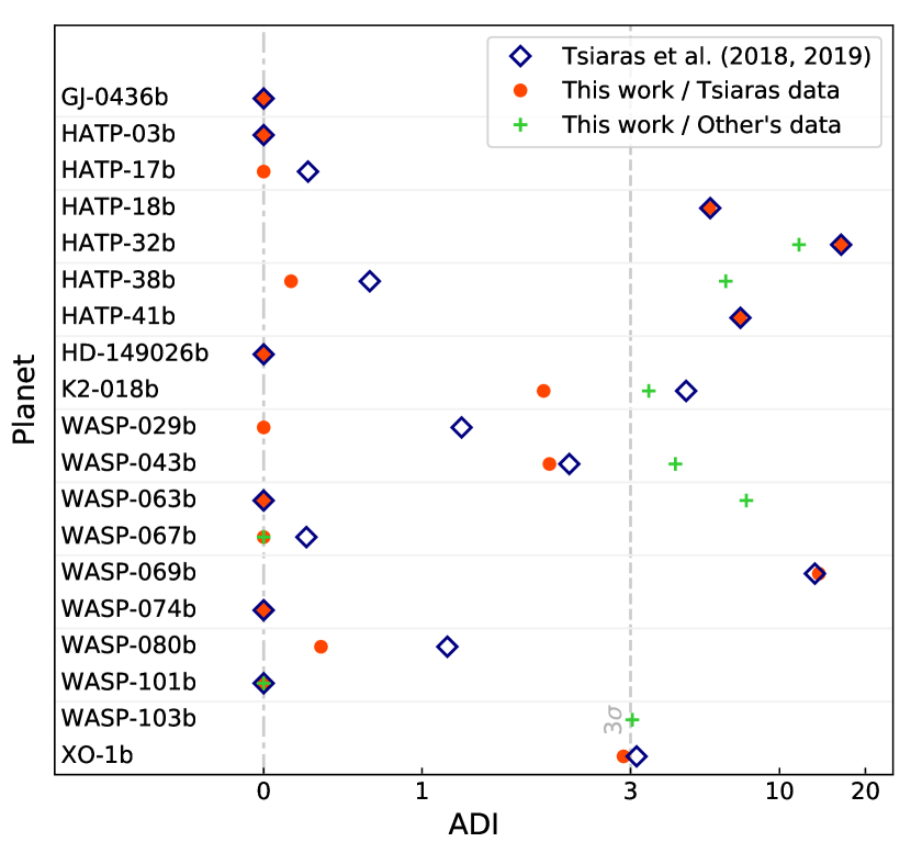
Figure 13: Atmospheric Detectability Index for the datasets in our sample. The red circles and green crosses show our estimation of the ADI values for the datasets from Tsiaras et al. (2018); Tsiaras et al. (2019) and other groups, respectively. The blue diamonds show the ADI values estimated by Tsiaras et al. (2018); Tsiaras et al. (2019). For our analyses, we have selected the lowest-BIC model for each dataset (see Tables 8–11). Note that the X axis is linear for $0<{\rm ADI}<1$ and logarithmic for $1<{\rm ADI}$. The vertical dashed line marks the ADI level where the flat (featureless) fit is rejected at a 3$\sigma$ significance.

4.3.1 H₂O Detection

To further assess the significance of the spectral features seen in our models, we compared these detections to a featureless model fit using the Atmospheric Detectability Index ${\rm ADI}=\max\,\{0,\log B\}$ (Tsiaras et al., 2018), where $\log B$ is the logarithmic Bayes factor (see, e.g., Raftery, 1995):

$$\log B=\frac{1}{2}({\rm BIC}_{i}-{\rm BIC_{flat}}),$$ (27)

where BICflat is the Bayesian information criterion of a flat-curve fit and BIC_i is the Bayesian information criterion of the best-fit model (for the optimal model setup according to Tables 8–11, i.e., the lowest-BIC model). Figure 13 shows our ADI values for the datasets in the sample. We find that 10 out of the 19 targets show strong evidence in favor of molecular features over a flat spectrum (${\rm ADI}\gtrsim 3$, which corresponds to the $3\sigma$ criterion of Tsiaras et al., 2018). In general, the targets that have multiple light-curve analyses show similar ADI values. However, there are exceptional cases like HAT-P-38b and WASP-63b, where each dataset produces widely different ADI values. These results suggest that although the WFC3/G141 data alone are often not sufficient to distinguish between different scenarios, these observations can still tell us whether there is evidence for molecular features in a statistically robust manner. For the rest of this section we will focus on the datasets with significant spectral feature detections (i.e., ${\rm ADI}\gtrsim 3$), since the datasets with ${\rm ADI}<3$ produced largely unconstrained posteriors that provide little insight. Table 7 shows our retrieval results for the 10 targets with ${\rm ADI}\gtrsim 3$ (the highest ADI dataset and lowest-BIC cloudy model for each target). Figure 14 shows the marginal posterior of $X_{\rm H2O}$, the only molecule consistently detected. Due to the degeneracy between the model parameters the $X_{\rm H2O}$ posteriors are asymmetric and the credible intervals often span several orders of magnitude. Since the amplitude of the 1.4-$\mu$m H₂O feature is often smaller than that of a clear solar-composition atmosphere, most posteriors in Fig. 14 show either very high $X_{\rm H2O}$ values (small scale-height atmospheres), broad solar-to-supersolar $X_{\rm H2O}$ values correlated with the $p_{\rm top}$ parameter (cloudy atmospheres), sub-solar $X_{\rm H2O}$ values ($H$2$O$-depleted atmospheres), or a combination of them. In particular, HAT-P-38b, WASP-69b, and WASP-103b show bimodal $X_{\rm H2O}$ posterior distributions. The only other molecule observed in these datasets is HCN for the WASP-63b analysis of Kilpatrick et al. (2018). For K2-18b, WASP-43b, and WASP-103b, which have Spitzer observations, we obtained flat or upper-limit posteriors for $X_{\rm CO}$, $X_{\rm CO2}$, and $X_{\rm CH4}$ (we will discuss these constraints in more detail in Section 4.3.2).

Table 7: WFC3 Retrieval Results for planets with ${\rm ADI}\gtrsim 3$.

Dataset	$T({\rm K})$	$R_{\rm planet}$ ($R_{\rm Jup}$)	$\log_{10}(X_{\rm H2O})$	$\log_{10}(X_{\rm HCN})$	$\log_{10}(p_{\rm top})$
HATP-18b Tsiaras	$423_{-261}^{+149}$	$0.952_{-0.007}^{+0.004}$	$-0.44_{-1.07}^{+0.40}$	$\cdots$	$-1.07_{-1.13}^{+2.76}$
HATP-32b Tsiaras	$643_{-192}^{+321}$	$1.797_{-0.019}^{+0.006}$	$-0.94_{-2.13}^{+0.24}$	$\cdots$	$-1.19_{-1.36}^{+2.55}$
HATP-38b Bruno	$1460_{-215}^{+40}$	$0.841_{-0.041}^{+0.004}$	$-5.71_{-0.43}^{+0.59}$ and $-0.77_{-0.78}^{+0.53}$	$\cdots$	$0.46_{-4.34}^{+1.40}$
HATP-41b Tsiaras	$1392_{-418}^{+635}$	$1.619_{-0.025}^{+0.043}$	$-0.93_{-3.90}^{+0.23}$	$\cdots$	$-1.74_{-2.56}^{+1.08}$
K2-18b Benneke	$352_{-142}^{+30}$	$0.246_{-0.001}^{+0.002}$	$-0.87_{-2.47}^{+0.31}$	$\cdots$	$-0.91_{-0.94}^{+2.00}$
WASP-43b Stevenson	$502_{-144}^{+156}$	$1.035_{-0.001}^{+0.001}$	$-2.16_{-1.29}^{+0.96}$	$\cdots$	$0.01_{-0.68}^{+1.82}$
WASP-63b Kilpatrick	$569_{-169}^{+530}$	$1.418_{-0.031}^{+0.014}$	$-3.82_{-1.34}^{+1.33}$	$-3.21_{-1.36}^{+1.67}$	$-1.07_{-2.54}^{+2.39}$
WASP-69b Tsiaras	$154_{-45}^{+109}$	$1.017_{-0.001}^{+0.001}$	$-3.76_{-0.80}^{+1.01}$ and $-0.40_{-0.24}^{+0.20}$	$\cdots$	$2.28_{-3.86}^{+0.32}$
WASP-103b Kreidberg	$2853_{-725}^{+127}$	$1.615_{-0.069}^{+0.008}$	$-5.60_{-0.65}^{+1.01}$ and $-1.27_{-1.59}^{+0.57}$	$\cdots$	$0.71_{-1.75}^{+1.29}$
XO-1b Tsiaras	$714_{-233}^{+352}$	$1.195_{-0.010}^{+0.002}$	$-1.02_{-1.79}^{+0.32}$	$\cdots$	$0.79_{-2.05}^{+1.08}$

• The reported values correspond to the marginal posterior distribution’s mode and boundaries of the 68% HPD credible intervals.

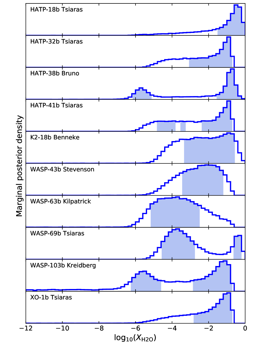
Figure 14: H₂O volume mixing ratio marginal posterior for the targets with ${\rm ADI}\gtrsim 3$ (Fig. 13). The shaded areas denote the 68% highest-posterior-density credible intervals.

4.3.2 Comparison to Literature

The ADI metric allows us to make a global comparison of our retrieval results with those of Tsiaras et al. (2018); Tsiaras et al. (2019). Note that ADI is a model-dependent metric; even though two analyses may be fitting the same data, we do not necessarily expect to find the same ADI results if the underlying models differ. Nevertheless, the ADI is a simple metric that can tell whether different analyses find evidence for spectral features in a same dataset. Figure 13 shows that the ADI values found in this work agree relatively well with those of Tsiaras et al. for most of the samples, in particular for the most significant detections where ${\rm ADI}\gtrsim 3$. For individual retrieval analyses we see a good agreement between our results and those from the literature, as long as both analyses adopt a similar set of assumptions (i.e., same models to parameterize the atmosphere, same set of parameters, and similar parameter priors and boundaries). We can make a direct comparison with the HAT-P-32b, HAT-P-38b, and WASP-67b analyses (Damiano et al., 2017; Bruno et al., 2018), which have published pairwise posterior distributions and adopt the same atmospheric parameterization as we do. In these cases, both retrieval analyses find consistent best-fitting solutions, posterior distributions, and correlations between the parameters. Notably, HAT-P-38b shows seemingly anomalously high values for the retrieved temperature (see Fig. 8 or Table 7). This could be attributed to systematics in the reduced data, reported by Bruno et al. (2018), particularly for the longer-wavelength data points. Benneke et al. (2019) retrieved the WFC3 and Spitzer spectrum of K2-18b by fitting an isothermal temperature, a gray cloud deck, and the volume mixing ratios of H₂O, CH₄, CO, CO₂, NH₃, HCN, and N₂. Qualitatively, our retrieval results match those of Benneke et al. (2019), finding a strong correlation between $X_{\rm H2O}$ and the cloud top pressure (see their Fig. 4). We obtained posterior boundaries fairly similar to those of Benneke et al. (2019); at a 1$\sigma$ significance we constrained $X_{\rm H2O}$ between $1\times 10^{-3}$ and $0.3$ (they, between 3$\times 10^{-4}$ and 0.1) and ${p_{\rm top}}$ between 2$\times 10^{-2}$ and 4 bar (they, between 8$\times 10^{-3}$ and 0.1 bar). For the remaining molecular abundances we obtained 2$\sigma$ upper limits of 0.04, 0.01, 8$\times 10^{-4}$, and 0.09 for $X_{\rm CO}$, $X_{\rm CO2}$, $X_{\rm CH4}$, and $X_{\rm N2}$, respectively, whereas Benneke et al. (2019) found upper limits of 0.07, 0.02, 2$\times 10^{-3}$, and 0.1, respectively. The H₂O and cloud detection make K2-18b an interesting candidate for further characterization, since the planet receives a stellar insulation similar to that of the Earth, enabling the possibility to characterize water clouds. Kreidberg et al. (2014) analyzed the WFC3 transmission spectrum of WASP-43b. Their retrieval parameterization included an isothermal temperature, a gray cloud deck, a reference pressure level ($\log p_{0}$), and the volume mixing ratios of H₂O, CH₄, CO, and CO₂. This modeling setup is equivalent to ours, except that they fit for a reference pressure level ($\log p_{0}$) instead of a reference radius ($R_{\rm p}$). However, as mentioned in Section 3.4, Welbanks & Madhusudhan (2019) showed that fixing $R_{\rm p}$ and fitting for $\log p_{0}$ is equivalent to fixing $\log p_{0}$ and fitting for $R_{\rm p}$. Qualitatively, our retrieval posteriors show the same correlations found by Kreidberg et al. (2014), with $X_{\rm H2O}$ correlating mainly with the reference $R_{\rm p}$–$p_{0}$ point. The cloud top pressure is generally constrained below the pressures probed by the observations. Quantitatively, our 1$\sigma$ credible intervals overlap with those of Kreidberg et al. (2014), though our ranges are slightly offset from theirs. We constrained $X_{\rm H2O}$ between $4\times 10^{-4}$ and $0.06$, $T$ between 360 and 660 K, and ${p_{\rm top}}>0.2$ bar (at 1$\sigma$); whereas Kreidberg et al. (2014) constrained $X_{\rm H2O}$ between 3$\times 10^{-5}$ and 5$\times 10^{-3}$, T between 510 and 780 K, and ${p_{\rm top}}>0.1$ bar. Kilpatrick et al. (2018) present a further example of consistent retrieval results between different frameworks. They studied the HST WFC3/G141 transmission spectrum of WASP-63b, comparing our retrieval framework with CHIMERA (Line et al., 2016), TauREx (Waldmann, 2016), and POSEIDON (MacDonald & Madhusudhan, 2017). Even though the different frameworks used different statistical samplers, cross section databases, and atmospheric parameterizations, all four retrieval analyses produced consistent results, finding a strong detection of the H₂O feature. The amplitude of the H₂O features is however muted when compared to that of a clear solar-composition atmospheric model. A weaker detection of an absorption feature is also observed at 1.55 $\mu$m. This feature is consistent with a super-solar abundance of HCN that would require the presence of strong disequilibrium-chemistry processes like quenching and photochemistry (see, e.g., Moses, 2014). For WASP-103b it is not possible to make a direct comparison with Kreidberg et al. (2018a), since they did not retrieve the transmission spectrum, but rather analyzed the phase-curve emission spectrum of the planet. Under the assumption of thermochemical and radiative-convective equilibrium, they found that WASP-103b does not show H₂O spectral features in emission, attributed to H₂O dissociation or additional absorption from other species like H^-. The emission spectra are consistent with blackbody emission ranging from 1900 K (at the night side) to 2900 K (at the day side). From our transmission spectrum retrieval, we found a temperature posterior that is consistent with the range of temperatures obtained by Kreidberg et al. (2018a), although very broad, $T\sim$2100–3000 K. Our retrieved H₂O composition is affected by strong parameter correlations as well as by the choice of retrieval parameters: when we included all abundance free parameters in the retrieval ($X_{\rm H2O}$, $X_{\rm CO}$, $X_{\rm CO2}$, $X_{\rm CH4}$, and $X_{\rm N2}$) we obtained a broad $X_{\rm H2O}$ posterior peaking at super-solar values (see Fig. 11); however, when we retrieved the abundance of only H₂O the $X_{\rm H2O}$ posterior showed a bimodal $X_{\rm H2O}$ distribution, peaking at sub-solar and super-solar compositions (see Fig. 14 and Table 7). Our lower H₂O-abundance solution mode ($X_{\rm H2O}\approx 3\times 10^{-6}$) is more consistent with the emission models of Kreidberg et al. (2018a). Although, this should not be considered a direct comparison since transmission and emission spectroscopy follow a different geometry and, thus, probe different regions in the atmosphere. Fisher & Heng (2018) performed a comprehensive analysis of 38 WFC3 exoplanet transmission spectra, with several targets in common with those in our sample. Their atmospheric models fit the same components as ours, however, their formulation of the radiative transfer equation differs from ours. They employed a semi-analytic model evaluating physical properties at a single pressure level. They also, tested a suit of clear, gray, and non-gray cloudy models. For the molecular cross sections, they included the contribution from H₂O, HCN, and NH₃. Fisher & Heng (2018) found that for the majority of targets the Bayesian evidence favors isothermal temperature profiles and the presence of gray clouds. H₂O is the only molecule consistently detected. They found no evidence of trends between the retrieved H₂O abundances and other physical parameters, like the planetary mass or temperature. Considering the targets in common, our retrieved $X_{\rm H2O}$ values are generally consistent (within the 68% credible intervals) with those of Fisher & Heng (2018). We also observed no clear trend between physical parameters. Overall, the main conclusion from these analyses is that H₂O is the only molecule consistently detected with WFC3 transmission data. However, with only WFC3 observations, the $X_{\rm H2O}$ posterior distributions are highly correlated with other atmospheric parameters, like the cloud top pressure or the pressure–radius reference point. These degeneracies lead to broad, poorly constrained H₂O abundances.

5 Summary

In this article, we presented the Pyrat Bay framework for exoplanet atmospheric characterization. The modular design of Pyrat Bay allows the users to carry out specific or general atmospheric modeling tasks, that is, compute 1D atmospheric models, sample line-by-line molecular cross sections, compute transmission or emission spectra, and perform Bayesian atmospheric retrievals. Pyrat Bay is an open-source (GNU GPL v2 license), well documented, and thoroughly tested Python package (compatible with Python versions 3.6 and above). The code is readily available for installation from PyPI (

pip install pyratbay}) or conda
(\mintinline

shellconda install -c conda-forge pyratbay). The source code is hosted at http://pcubillos.github.io/pyratbay and the documentation is located at https://pyratbay.readthedocs.io. We benchmarked the individual components of the Pyrat Bay framework (line sampling, spectral synthesis, and atmospheric retrieval) by successfully reproducing the line-by-line sampling cross sections of Chubb et al. (2021), by reproducing petitRADTRANS transmission and emission spectra, and by retrieving synthetic Ariel-like transmission and emission spectra generated with TauREx. We also re-analyzed with Pyrat Bay the 0.3–5.5 $\mu$m transmission spectrum of HD 209458 b studied by MacDonald & Madhusudhan (2017) and Pinhas et al. (2019), finding a good agreement with them for most retrieved parameters. We also initiated a population study of the existing exoplanet transmission spectra obtained from space-based observatories, where we applied a standardized retrieval approach. As a starting point, in this article we considered the targets without observations at $\lambda<1$ $\mu$m. This sample consists of 26 datasets of 19 different systems, most of them observed exclusively with the HST WFC3/G141 detector (1.1–1.7 $\mu$m). Thus, we focused our analysis on the characterization of the H₂O absorption band centered at $1.4$ $\mu$m. A Bayesian model comparison indicates that 9 out of the 19 systems show strong evidence for H₂O molecular features in the data. However, it is not possible to obtain precise H₂O abundance constraints. The limited wavelength coverage and signal-to-noise ratio of the data do not allow us to distinguish cloudy from high metal-mass-fraction scenarios ($\Delta$BIC<2, see Tables 8–11), leading to degenerate posterior distributions. Our results are well in agreement with previous studies of these datasets, particularly when both retrieval analyses adopt similar assumptions. Follow up articles will present the atmospheric retrieval analysis of planets that have been observed in transmission at shorter wavelengths. Ongoing development of the Pyrat Bay framework includes self-consistent radiative- and thermochemical-equilibrium atmospheric modeling, posterior sampling under thermochemical equilibrium, sophisticated kinetic and thermal-stability cloud models, and physically-consistent multi-dimensional retrievals for phase-curve observations. In conclusion, current atmospheric retrievals rely on a number of modeling choices, either to simplify the already computationally intensive calculations (e.g., assuming 1D atmospheric parameterizations) or to simplify the parameter space exploration (e.g., assuming thermochemical-equilibrium abundances). These choices can have a significant, or even dominating, influence on the retrieval results. Carrying out independent retrieval analyses of a given observation help us test the impact of the model assumptions, making our interpretation of the observation more robust. Despite the limited characterizing power of the WFC3/G141 grism alone, these observations are highly valuable to determine the targets with the most favorable conditions for further characterization. We expect that better targets with stronger features and additional spectral coverage will enable us to perform more in-depth population studies (e.g., Sing et al., 2016; Crossfield & Kreidberg, 2017). In particular, Pinhas et al. (2019) showed that by combining infrared WFC3 data with optical HST/STIS data helps to break the degeneracy between the reference pressure–radius point and the H₂O abundance. For the transmission spectrum of HD 209458 b, the retrieval of the combined STIS and WFC3 data lead to an uncorrelated $X_{\rm H2O}$ constraint, three times tighter than when retrieving the WFC3 data alone. Observations from future telescopes (e.g., JWST or Ariel), with better sensitivity, wavelength coverage, and spectral resolution will be crucial to construct a more robust picture of the physical processes dominating exoplanet atmospheres. For example, Greene et al. (2016) estimated that JWST will be able to discriminate between cloudy and high metal-mass-fraction atmospheres. JWST observations between 1–2.5 $\mu$m will often suffice to constrain the volume mixing ratios of dominant molecular species, C/O ratios, and metallicity of clear planetary atmospheres. A broader wavelength coverage (1–11 $\mu$m) provides significantly better constraints and has the potential to constrain the properties of cloudy atmospheres.

Data Availability

To allow the readers to fully reproduce the analyses presented in this article, we provide a research compendium available in Zenodo at https://doi.org/10.5281/zenodo.4749530.

Appendix A Model Comparison Statistics

Tables 8–11 show the model-comparison statistics for the WFC3 sample.

Table 8: Model comparison statistics. $\Delta$BIC is the difference in BIC with respect to the lowest-BIC (optimal) model for the given dataset. $N_{\rm free}$ is the number of free retrieval parameters.

GJ-436b Tsiaras
ID	Free parameters	$N_{\rm free}$	$\Delta$BIC	$\chi^{2}_{\rm red}$
M1	$T$, $R_{\rm p}$, H2O, $p_{\rm top}$	4	$6.8$	$1.33\pm 0.38$
M2	$T$, $R_{\rm p}$, H2O, [M/H]	4	$6.8$	$1.33\pm 0.38$
M3	$T$, $R_{\rm p}$, H2O, [M/H], $p_{\rm top}$	5	$9.7$	$1.43\pm 0.39$
M0	Flat fit	1	$0.0$	$1.21\pm 0.34$
HATP-3b Tsiaras
ID	Free parameters	$N_{\rm free}$	$\Delta$BIC	$\chi^{2}_{\rm red}$
M1	$T$, $R_{\rm p}$, H2O, $p_{\rm top}$	4	$7.6$	$1.07\pm 0.38$
M2	$T$, $R_{\rm p}$, H2O, [M/H]	4	$8.2$	$1.11\pm 0.38$
M3	$T$, $R_{\rm p}$, H2O, [M/H], $p_{\rm top}$	5	$10.5$	$1.15\pm 0.39$
M0	Flat fit	1	$0.0$	$0.94\pm 0.34$
HATP-17b Tsiaras
ID	Free parameters	$N_{\rm free}$	$\Delta$BIC	$\chi^{2}_{\rm red}$
M1	$T$, $R_{\rm p}$, H2O, $p_{\rm top}$	4	$5.1$	$1.34\pm 0.38$
M2	$T$, $R_{\rm p}$, H2O, [M/H]	4	$5.1$	$1.34\pm 0.38$
M3	$T$, $R_{\rm p}$, H2O, [M/H], $p_{\rm top}$	5	$8.0$	$1.45\pm 0.39$
M0	Flat fit	1	$0.0$	$1.32\pm 0.34$
HATP-18b tsiaras
ID	Free parameters	$N_{\rm free}$	$\Delta$BIC	$\chi^{2}_{\rm red}$
M1	$T$, $R_{\rm p}$, H2O, $p_{\rm top}$	4	$0.0$	$1.05\pm 0.38$
M2	$T$, $R_{\rm p}$, H2O, [M/H]	4	$0.0$	$1.05\pm 0.38$
M3	$T$, $R_{\rm p}$, H2O, [M/H], $p_{\rm top}$	5	$2.9$	$1.13\pm 0.39$
M0	Flat fit	1	$11.3$	$2.04\pm 0.34$
HATP-32b Damiano
ID	Free parameters	$N_{\rm free}$	$\Delta$BIC	$\chi^{2}_{\rm red}$
M1	$T$, $R_{\rm p}$, H2O, $p_{\rm top}$	4	$0.0$	$1.38\pm 0.35$
M2	$T$, $R_{\rm p}$, H2O, [M/H]	4	$0.0$	$1.38\pm 0.35$
M3	$T$, $R_{\rm p}$, H2O, [M/H], $p_{\rm top}$	5	$3.0$	$1.48\pm 0.37$
M0	Flat fit	1	$23.4$	$2.87\pm 0.32$
HATP-32b Tsiaras
ID	Free parameters	$N_{\rm free}$	$\Delta$BIC	$\chi^{2}_{\rm red}$
M1	$T$, $R_{\rm p}$, H2O, $p_{\rm top}$	4	$0.0$	$0.92\pm 0.38$
M2	$T$, $R_{\rm p}$, H2O, [M/H]	4	$0.0$	$0.92\pm 0.38$
M3	$T$, $R_{\rm p}$, H2O, [M/H], $p_{\rm top}$	5	$2.9$	$0.99\pm 0.39$
M0	Flat fit	1	$33.0$	$3.21\pm 0.34$
HATP-38b bruno
ID	Free parameters	$N_{\rm free}$	$\Delta$BIC	$\chi^{2}_{\rm red}$
M1	$T$, $R_{\rm p}$, H2O, $p_{\rm top}$	4	$0.0$	$1.33\pm 0.43$
M2	$T$, $R_{\rm p}$, H2O, [M/H]	4	$0.0$	$1.33\pm 0.43$
M3	$T$, $R_{\rm p}$, H2O, [M/H], $p_{\rm top}$	5	$2.8$	$1.47\pm 0.45$
M0	Flat fit	1	$13.0$	$2.55\pm 0.38$

Table 9: Model comparison statistics (continuation).

HATP-38b tsiaras
ID	Free parameters	$N_{\rm free}$	$\Delta$BIC	$\chi^{2}_{\rm red}$
M1	$T$, $R_{\rm p}$, H2O, $p_{\rm top}$	4	$0.0$	$0.80\pm 0.38$
M2	$T$, $R_{\rm p}$, H2O, [M/H]	4	$0.1$	$0.81\pm 0.38$
M3	$T$, $R_{\rm p}$, H2O, [M/H], $p_{\rm top}$	5	$3.0$	$0.87\pm 0.39$
M0	Flat fit	1	$0.3$	$1.19\pm 0.34$
HATP-41b Tsiaras
ID	Free parameters	$N_{\rm free}$	$\Delta$BIC	$\chi^{2}_{\rm red}$
M1	$T$, $R_{\rm p}$, H2O, $p_{\rm top}$	4	$0.0$	$0.32\pm 0.38$
M2	$T$, $R_{\rm p}$, H2O, [M/H]	4	$1.6$	$0.43\pm 0.38$
M3	$T$, $R_{\rm p}$, H2O, [M/H], $p_{\rm top}$	5	$2.9$	$0.34\pm 0.39$
M0	Flat fit	1	$14.5$	$1.62\pm 0.34$
HD 149026 b Tsiaras
ID	Free parameters	$N_{\rm free}$	$\Delta$BIC	$\chi^{2}_{\rm red}$
M1	$T$, $R_{\rm p}$, H2O, $p_{\rm top}$	4	$4.1$	$0.85\pm 0.38$
M2	$T$, $R_{\rm p}$, H2O, [M/H]	4	$4.4$	$0.87\pm 0.38$
M3	$T$, $R_{\rm p}$, H2O, [M/H], $p_{\rm top}$	5	$6.9$	$0.91\pm 0.39$
M0	Flat fit	1	$0.0$	$0.97\pm 0.34$
K2-18b Benneke
ID	Free parameters	$N_{\rm free}$	$\Delta$BIC	$\chi^{2}_{\rm red}$
M1	$T$, $R_{\rm p}$, H2O, $p_{\rm top}$	4	$0.0$	$0.57\pm 0.37$
M2	$T$, $R_{\rm p}$, H2O, [M/H]	4	$0.0$	$0.57\pm 0.37$
M3	$T$, $R_{\rm p}$, H2O, [M/H], $p_{\rm top}$	5	$2.8$	$0.60\pm 0.38$
M4	$T$, $R_{\rm p}$, H2O, CO, CO2, CH4, $p_{\rm top}$	7	$8.9$	$0.72\pm 0.41$
M5	$T$, $R_{\rm p}$, H2O, CO, CO2, CH4, [M/H]	7	$9.0$	$0.73\pm 0.41$
M6	$T$, $R_{\rm p}$, H2O, CO, CO2, CH4, [M/H], $p_{\rm top}$	8	$11.7$	$0.77\pm 0.43$
M0	Flat fit	1	$7.0$	$1.35\pm 0.33$
K2-18b tsiaras
ID	Free parameters	$N_{\rm free}$	$\Delta$BIC	$\chi^{2}_{\rm red}$
M1	$T$, $R_{\rm p}$, H2O, $p_{\rm top}$	4	$0.0$	$0.98\pm 0.39$
M2	$T$, $R_{\rm p}$, H2O, [M/H]	4	$0.4$	$1.01\pm 0.39$
M3	$T$, $R_{\rm p}$, H2O, [M/H], $p_{\rm top}$	5	$2.8$	$1.06\pm 0.41$
M0	Flat fit	1	$4.0$	$1.57\pm 0.35$
WASP-29b Tsiaras
ID	Free parameters	$N_{\rm free}$	$\Delta$BIC	$\chi^{2}_{\rm red}$
M1	$T$, $R_{\rm p}$, H2O, $p_{\rm top}$	4	$2.4$	$0.58\pm 0.38$
M2	$T$, $R_{\rm p}$, H2O, [M/H]	4	$2.4$	$0.58\pm 0.38$
M3	$T$, $R_{\rm p}$, H2O, [M/H], $p_{\rm top}$	5	$5.3$	$0.62\pm 0.39$
M0	Flat fit	1	$0.0$	$0.85\pm 0.34$

Table 10: Model comparison statistics (continuation).

WASP-43b Stevenson
ID	Free parameters	$N_{\rm free}$	$\Delta$BIC	$\chi^{2}_{\rm red}$
M1	$T$, $R_{\rm p}$, H2O, $p_{\rm top}$	4	$0.0$	$2.64\pm 0.32$
M2	$T$, $R_{\rm p}$, H2O, [M/H]	4	$0.2$	$2.65\pm 0.32$
M3	$T$, $R_{\rm p}$, H2O, [M/H], $p_{\rm top}$	5	$3.2$	$2.78\pm 0.32$
M4	$T$, $R_{\rm p}$, H2O, CO, CO2, CH4, $p_{\rm top}$	7	$9.6$	$3.11\pm 0.34$
M5	$T$, $R_{\rm p}$, H2O, CO, CO2, CH4, [M/H]	7	$9.7$	$3.12\pm 0.34$
M6	$T$, $R_{\rm p}$, H2O, CO, CO2, CH4, [M/H], $p_{\rm top}$	8	$12.8$	$3.31\pm 0.35$
M0	Flat fit	1	$8.6$	$3.09\pm 0.29$
WASP-43b Tsiaras
ID	Free parameters	$N_{\rm free}$	$\Delta$BIC	$\chi^{2}_{\rm red}$
M1	$T$, $R_{\rm p}$, H2O, $p_{\rm top}$	4	$0.0$	$1.53\pm 0.38$
M2	$T$, $R_{\rm p}$, H2O, [M/H]	4	$0.0$	$1.53\pm 0.38$
M3	$T$, $R_{\rm p}$, H2O, [M/H], $p_{\rm top}$	5	$2.9$	$1.64\pm 0.39$
M0	Flat fit	1	$3.6$	$1.98\pm 0.34$
WASP-63b Kilpatrick
ID	Free parameters	$N_{\rm free}$	$\Delta$BIC	$\chi^{2}_{\rm red}$
M1	$T$, $R_{\rm p}$, H2O, $p_{\rm top}$	4	$5.5$	$2.04\pm 0.43$
M2	$T$, $R_{\rm p}$, H2O, [M/H]	4	$6.0$	$2.08\pm 0.43$
M3	$T$, $R_{\rm p}$, H2O, [M/H], $p_{\rm top}$	5	$8.2$	$2.24\pm 0.45$
M4	$T$, $R_{\rm p}$, H2O, HCN, $p_{\rm top}$	5	$0.0$	$1.42\pm 0.45$
M5	$T$, $R_{\rm p}$, H2O, HCN, [M/H]	5	$1.9$	$1.62\pm 0.45$
M6	$T$, $R_{\rm p}$, H2O, HCN, [M/H], $p_{\rm top}$	6	$2.7$	$1.58\pm 0.47$
M0	Flat fit	1	$15.3$	$2.88\pm 0.38$
WASP-63b Tsiaras
ID	Free parameters	$N_{\rm free}$	$\Delta$BIC	$\chi^{2}_{\rm red}$
M1	$T$, $R_{\rm p}$, H2O, $p_{\rm top}$	4	$3.6$	$0.99\pm 0.38$
M2	$T$, $R_{\rm p}$, H2O, [M/H]	4	$4.0$	$1.02\pm 0.38$
M3	$T$, $R_{\rm p}$, H2O, [M/H], $p_{\rm top}$	5	$6.5$	$1.07\pm 0.39$
M1	$T$, $R_{\rm p}$, H2O, HCN, [M/H], $p_{\rm top}$	6	$8.8$	$1.11\pm 0.41$
M0	Flat fit	1	$0.0$	$1.11\pm 0.34$
WASP-67b Bruno
ID	Free parameters	$N_{\rm free}$	$\Delta$BIC	$\chi^{2}_{\rm red}$
M1	$T$, $R_{\rm p}$, H2O, $p_{\rm top}$	4	$1.3$	$1.32\pm 0.41$
M2	$T$, $R_{\rm p}$, H2O, [M/H]	4	$1.3$	$1.32\pm 0.41$
M3	$T$, $R_{\rm p}$, H2O, [M/H], $p_{\rm top}$	5	$4.1$	$1.44\pm 0.43$
M0	Flat fit	1	$0.0$	$1.52\pm 0.37$
WASP-67b Tsiaras
ID	Free parameters	$N_{\rm free}$	$\Delta$BIC	$\chi^{2}_{\rm red}$
M1	$T$, $R_{\rm p}$, H2O, $p_{\rm top}$	4	$2.5$	$0.57\pm 0.38$
M2	$T$, $R_{\rm p}$, H2O, [M/H]	4	$2.5$	$0.57\pm 0.38$
M3	$T$, $R_{\rm p}$, H2O, [M/H], $p_{\rm top}$	5	$5.4$	$0.62\pm 0.39$
M0	Flat fit	1	$0.0$	$0.84\pm 0.34$

Table 11: Model comparison statistics (continuation).

WASP-69b tsiaras
ID	Free parameters	$N_{\rm free}$	$\Delta$BIC	$\chi^{2}_{\rm red}$
M1	$T$, $R_{\rm p}$, H2O, $p_{\rm top}$	4	$0.1$	$1.65\pm 0.38$
M2	$T$, $R_{\rm p}$, H2O, [M/H]	4	$0.0$	$1.65\pm 0.38$
M3	$T$, $R_{\rm p}$, H2O, [M/H], $p_{\rm top}$	5	$2.8$	$1.77\pm 0.39$
M0	Flat fit	1	$27.5$	$3.48\pm 0.34$
WASP-74b Tsiaras
ID	Free parameters	$N_{\rm free}$	$\Delta$BIC	$\chi^{2}_{\rm red}$
M1	$T$, $R_{\rm p}$, H2O, $p_{\rm top}$	4	$2.9$	$0.89\pm 0.38$
M2	$T$, $R_{\rm p}$, H2O, [M/H]	4	$2.8$	$0.89\pm 0.38$
M3	$T$, $R_{\rm p}$, H2O, [M/H], $p_{\rm top}$	5	$5.7$	$0.96\pm 0.39$
M0	Flat fit	1	$0.0$	$1.07\pm 0.34$
WASP-80b Tsiaras
ID	Free parameters	$N_{\rm free}$	$\Delta$BIC	$\chi^{2}_{\rm red}$
M1	$T$, $R_{\rm p}$, H2O, $p_{\rm top}$	4	$0.0$	$1.02\pm 0.39$
M2	$T$, $R_{\rm p}$, H2O, [M/H]	4	$0.3$	$1.04\pm 0.39$
M3	$T$, $R_{\rm p}$, H2O, [M/H], $p_{\rm top}$	5	$2.8$	$1.10\pm 0.41$
M0	Flat fit	1	$0.7$	$1.40\pm 0.35$
WASP-101b Tsiaras
ID	Free parameters	$N_{\rm free}$	$\Delta$BIC	$\chi^{2}_{\rm red}$
M1	$T$, $R_{\rm p}$, H2O, $p_{\rm top}$	4	$2.5$	$1.57\pm 0.38$
M2	$T$, $R_{\rm p}$, H2O, [M/H]	4	$2.4$	$1.57\pm 0.38$
M3	$T$, $R_{\rm p}$, H2O, [M/H], $p_{\rm top}$	5	$5.3$	$1.69\pm 0.39$
M0	Flat fit	1	$0.0$	$1.66\pm 0.34$
WASP-101b Wakeford
ID	Free parameters	$N_{\rm free}$	$\Delta$BIC	$\chi^{2}_{\rm red}$
M1	$T$, $R_{\rm p}$, H2O, $p_{\rm top}$	4	$5.0$	$2.76\pm 0.43$
M2	$T$, $R_{\rm p}$, H2O, [M/H]	4	$4.5$	$2.72\pm 0.43$
M3	$T$, $R_{\rm p}$, H2O, [M/H], $p_{\rm top}$	5	$7.6$	$3.03\pm 0.45$
M0	Flat fit	1	$0.0$	$2.40\pm 0.38$
WASP-103b Kreidberg
ID	Free parameters	$N_{\rm free}$	$\Delta$BIC	$\chi^{2}_{\rm red}$
M1	$T$, $R_{\rm p}$, H2O, $p_{\rm top}$	4	$0.0$	$1.40\pm 0.50$
M2	$T$, $R_{\rm p}$, H2O, [M/H]	4	$0.0$	$1.40\pm 0.50$
M3	$T$, $R_{\rm p}$, H2O, [M/H], $p_{\rm top}$	5	$2.5$	$1.60\pm 0.53$
M4	$T$, $R_{\rm p}$, H2O, CO, CO2, CH4, $p_{\rm top}$	7	$6.6$	$2.07\pm 0.63$
M5	$T$, $R_{\rm p}$, H2O, CO, CO2, CH4, [M/H]	7	$6.7$	$2.09\pm 0.63$
M6	$T$, $R_{\rm p}$, H2O, CO, CO2, CH4, [M/H], $p_{\rm top}$	8	$9.2$	$2.62\pm 0.71$
M0	Flat fit	1	$6.1$	$2.25\pm 0.43$
XO-1b Tsiaras
ID	Free parameters	$N_{\rm free}$	$\Delta$BIC	$\chi^{2}_{\rm red}$
M1	$T$, $R_{\rm p}$, H2O, $p_{\rm top}$	4	$0.0$	$0.76\pm 0.38$
M2	$T$, $R_{\rm p}$, H2O, [M/H]	4	$0.0$	$0.76\pm 0.38$
M3	$T$, $R_{\rm p}$, H2O, [M/H], $p_{\rm top}$	5	$2.9$	$0.82\pm 0.39$
M0	Flat fit	1	$5.7$	$1.47\pm 0.34$

References

- Abel et al. (2011) Abel M., Frommhold L., Li X., Hunt K. L. C., 2011, Journal of Physical Chemistry A, 115, 6805
- Al-Refaie et al. (2019) Al-Refaie A. F., Changeat Q., Waldmann I. P., Tinetti G., 2019, arXiv e-prints, p. arXiv:1912.07759
- Anderson et al. (2014) Anderson D. R., et al., 2014, MNRAS, 445, 1114
- Asplund et al. (2009) Asplund M., Grevesse N., Sauval A. J., Scott P., 2009, ARA&A, 47, 481
- Astropy Collaboration et al. (2013) Astropy Collaboration et al., 2013, A&A, 558, A33
- Astropy Collaboration et al. (2018) Astropy Collaboration et al., 2018, AJ, 156, 123
- Barstow et al. (2013) Barstow J. K., Aigrain S., Irwin P. G. J., Bowles N., Fletcher L. N., Lee J. M., 2013, MNRAS, 430, 1188
- Barstow et al. (2015) Barstow J. K., Aigrain S., Irwin P. G. J., Kendrew S., Fletcher L. N., 2015, MNRAS, 448, 2546
- Barstow et al. (2017) Barstow J. K., Aigrain S., Irwin P. G. J., Sing D. K., 2017, ApJ, 834, 50
- Barstow et al. (2020) Barstow J. K., Changeat Q., Garland R., Line M. R., Rocchetto M., Waldmann I. P., 2020, MNRAS, 493, 4884
- Baudino et al. (2017) Baudino J.-L., Mollière P., Venot O., Tremblin P., Bézard B., Lagage P.-O., 2017, ApJ, 850, 150
- Benneke (2015) Benneke B., 2015, arXiv e-prints, p. arXiv:1504.07655
- Benneke et al. (2017) Benneke B., et al., 2017, ApJ, 834, 187
- Benneke et al. (2019) Benneke B., et al., 2019, ApJ, 887, L14
- Blecic et al. (2016) Blecic J., Harrington J., Bowman M. O., 2016, ApJS, 225, 4
- Blecic et al. (2017) Blecic J., Dobbs-Dixon I., Greene T., 2017, ApJ, 848, 127
- Borysow (2002) Borysow A., 2002, A&A, 390, 779