AVA: Adversarial Vignetting Attack against Visual Recognition

Abstract

Vignetting is an inherit imaging phenomenon within almost all optical systems, showing as a radial intensity darkening toward the corners of an image. Since it is a common effect for the photography and usually appears as a slight intensity variation, people usually regard it as a part of a photo and would not even want to post-process it. Due to this natural advantage, in this work, we study the vignetting from a new viewpoint, i.e., adversarial vignetting attack (AVA), which aims to embed intentionally misleading information into the vignetting and produce a natural adversarial example without noise patterns. This example can fool the state-of-the-art deep convolutional neural networks (CNNs) but is imperceptible to human. To this end, we first propose the radial-isotropic adversarial vignetting attack (RI-AVA) based on the physical model of vignetting, where the physical parameters (e.g., illumination factor and focal length) are tuned through the guidance of target CNN models. To achieve higher transferability across different CNNs, we further propose radial-anisotropic adversarial vignetting attack (RA-AVA) by allowing the effective regions of vignetting to be radial-anisotropic and shape-free. Moreover, we propose the geometry-aware level-set optimization method to solve the adversarial vignetting regions and physical parameters jointly. We validate the proposed methods on three popular datasets, i.e., DEV, CIFAR10, and Tiny ImageNet, by attacking four CNNs, e.g., ResNet50, EfficientNet-B0, DenseNet121, and MobileNet-V2, demonstrating the advantages of our methods over baseline methods on both transferability and image quality.

1 Introduction

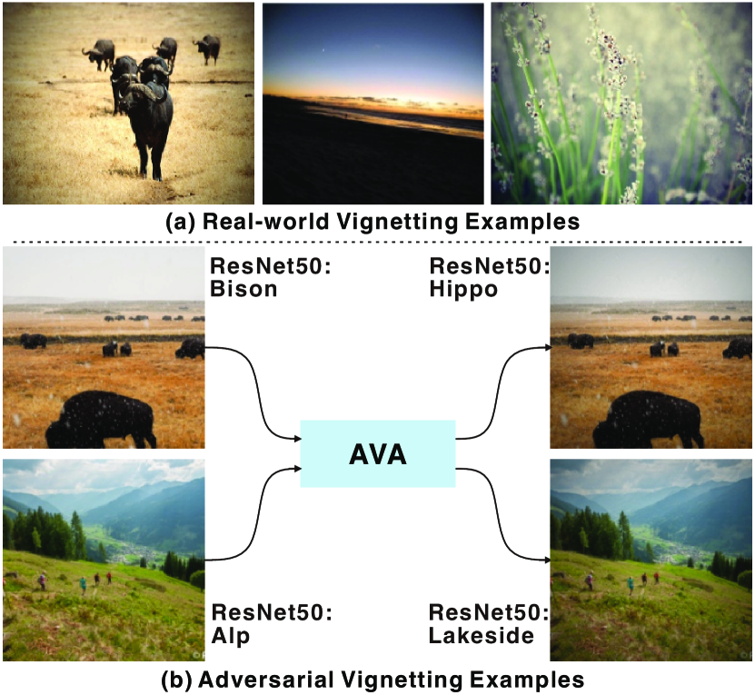
Figure 1: (a) shows three real vignetting images captured by cameras. (b) shows the adversarial examples produced by our adversarial vignetting attack (AVA), fooling the SOTA CNN ResNet50 with imperceptible property due to the realistic vignetting effects.

In photography, image vignetting is a common effect as a result of camera settings or lens limitations. It shows up as a gradually darkened transparent ring-shape mask towards the image border with continuous reduction of the image brightness or saturation Gonzalez et al. (2004). Vignetting often naturally occurs during the photo taking process. As categorized by Ray (2002), there are the following three main causes of vignetting for digital imaging: (1) mechanical vignetting, (2) optical vignetting, and (3) natural vignetting. Both mechanical vignetting and optical vignetting are somehow caused by the blockage of light. For example, the mechanical vignetting is caused by light emanated from off-axis scene being partially blocked by external objects such as lens hoods, and the optical vignetting is usually caused by the multiple element lens setting where the effective lens opening for off-axis incident light can be reduced. On the other hand, naturally vignetting is not due to light blockage, but rather by the law of illumination falloff where the light falloff is proportional to the 4-th power of the cosine of the angle at which the light particles hit the digital sensor. Sometimes, vignetting can also be applied on the digital image as an artistic post-processing step to draw people’s attention to the center portion of the photograph as depicted in Fig. 1(a).

Therefore, image vignetting can be capitalized to ideally hide adversarial attack information in a stealthy way for its ubiquity and naturalness in digital imaging. In this work, we propose a novel and stealthy attack method called the adversarial vignetting attack (AVA) that aims at embedding intentionally misleading information into the vignetting and producing a natural adversarial example without noise patterns, as depicted in Fig. 1(b). By first mathematically and physically model the image vignetting effect, we have proposed the radial-isotropic adversarial vignetting attack (RI-AVA) and the physical parameters such as the illumination factors and the focal length are tuned through the guidance of the target CNN models under attack. Next, by further allowing the effective regions of vignetting to be radial-anisotropic and shape-free, our proposed radial-anisotropic adversarial vignetting attack (RA-AVA) can achieve much higher transferability across different CNN models. Moreover, we have proposed the level-set-based optimization method, that is geometry-aware, to solve the adversarial vignetting regions and physical parameters jointly.

Through extensive experiments, we have validated the effectiveness of the proposed methods on three popular datasets, i.e., DEV Google (2017), CIFAR10 Krizhevsky et al. (2009), and Tiny ImageNet Stanford (2017), by attacking four CNNs, e.g., ResNet50 He et al. (2016), EfficientNet-B0 Tan and Le (2019), DenseNet121 Huang et al. (2017), and MobileNet-V2 Sandler et al. (2018). We have successfully demonstrated the advantages of our methods over strong baseline methods especially on transerferbility and image quality. To the best of our knowledge, this is the very first attempt to formulate stealthy adversarial attack by means of image vignetting and showcase both the feasibility and the effectiveness through extensive experiments.

2 Related Work

Adversarial noise attacks. Adversarial noise attacks aim to fool DNNs by adding imperceptible perturbations to the images. One of the most popular attack methods, i.e., fast gradient sign method (FGSM) Goodfellow et al. (2014), involves only one back propagation step in the process of calculating the gradient of cost function, enabling simple and fast adversarial example generation. Kurakin et al. (2016) proposes an improved version of FGSM, known as basic iteration method (BIM), which heuristically search for examples that are most likely to fool the classifier. Dong et al. (2018) proposes a broad class of momentum-based iterative algorithms to boost adversarial attacks. By integrating the momentum term into the iterative process for attacks, it can stabilize update directions and escape from poor local maxima during the iterations. Dong et al. (2019) further proposes a translation-invariant attack method to generate more transferable adversarial examples against the defense models. Adversarial noise attack will generate patterns that do not exist in reality, and our method is an early method of applying patterns that may be generated in natural optical systems to attacks.

Other adversarial attacks. In addition to traditional adversarial noise attacks, there are some methods that focus on sparse or real-life patterns. Croce and Hein (2019) proposes a new attack method to generate adversarial examples aiming at minimizing the $l_{0}$-distance to the original image. It allows pixels to change only in region of high variation and avoiding changes along axis-aligned edges, resulting in almost non-perceivable adversarial examples. Wong et al. (2019) proposes a new threat model for adversarial attacks based on the Wasserstein distance. The resulting algorithm can successfully attack image classification models, bringing traditional CIFAR10 models down to 3% accuracy within a Wasserstein ball with radius 0.1. Bhattad et al. (2019) introduces “unrestricted” perturbations that manipulate semantically meaningful image-based visual descriptors (e.g., color and texture) to generate effective and photorealistic adversarial examples. Guo et al. (2020b) proposes an adversarial attack method that can generate visually natural motion-blurred adversarial examples. Along similar lines, non-additive noise based adversarial attacks that focus on producing realistic degradation-like adversarial patterns have emerged in several recent studies, such as adversarial rain Zhai et al. (2020) and haze Gao et al. (2021), adversarial exposure for medical analysis Cheng et al. (2020b) and co-saliency detection problems Gao et al. (2020), adversarial bias field in medial imaging Tian et al. (2020), as well as adversarial denoising Cheng et al. (2020a) and face morphing Wang et al. (2020). These methods apply patterns that may be produced in reality such as color and texture to attack, but ignore the patterns that are generated naturally in the optical systems, which are also vitally important.

Vignetting correction methods. Research into vignetting correction has a long history. The Kang-Weiss model Kang and Weiss (2000) is established to simulate the vignetting effect. It proves that it is possible to calibrate a camera using just a flat, textureless Lambertian surface and constant illumination. Zheng et al. (2008) proposes a method for robustly determining the vignetting function in order to remove the vignetting given only a single image. Goldman (2010) further proposes a method to remove the vignetting from the images without resolving ambiguities or the previously known scale and gamma ambiguities. These works on correcting the vignetting effect provides a basis for us to model the vignetting effect. Inspired by these work, we will capitalize the vignetting effect as a means of an adversarial attack.

3 Adversarial Vignetting Attack (AVA)

Vignetting effect is related to numerous factors, e.g., angle-variant light across camera sensor, intrinsic lens characteristics, and physical occlusions. There are several works studying how to model the vignetting including empirical-based Goldman (2010); Yu (2004) and physical-based methods Asada et al. (1996); Kang and Weiss (2000). In particular, Kang and Weiss Kang and Weiss (2000) proposes a physical-based method that models vignetting via physically meaningful parameters (e.g., off-axis illumination, light path obstruction, tilt effects), allowing better understanding of the influence from real-world environments (e.g., camera setups or physical occlusion) to the final results. In this section, we start from the physical model of vignetting effects Kang and Weiss (2000) and propose two adversarial vignetting attacks based on this model with an level-set-based optimization.

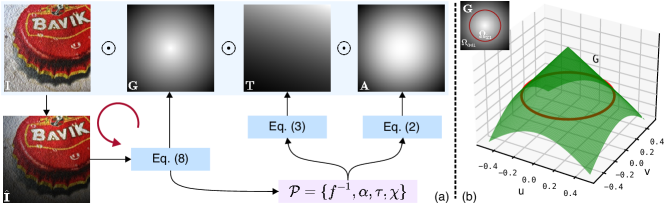
Figure 2: (a) shows the whole process of RA-AVA. (b) shows the 3D surface of the initialized $\mathbf{G}$. The red line is the curve splitting the image to 2 parts, i.e., $\Omega_{\text{in}}$ and $\Omega_{\text{out}}$.

3.1 Physical Model of Vignetting

Given a clean image $\mathbf{I}$, we aim to simulate the vignetting image via $\hat{\mathbf{I}}=\mathbf{I}\odot\mathbf{V}$ where $\mathbf{V}$ is a matrix having the same size with $\mathbf{I}$ and represents the vignetting effects, and $\odot$ denotes the pixel-wise multiplication. We model the vignetting from three aspects, i.e., off-axis illumination factor $\mathbf{A}$, geometric factor $\mathbf{G}$, and a tilt factor $\mathbf{T}$ Kang and Weiss (2000). All three factors are pixel-wise and have the same size with the original image. Then, the vignetting effects can be also represented as

$$\mathbf{V}=\mathbf{A}\odot\mathbf{G}\odot\mathbf{T}.$$ (1)

Intuitively, $\mathbf{A}$ describes the phenomenon of the illumination in the image that is darkened with distance away from the image center Kang and Weiss (2000), defined as

$$\mathbf{A}=\frac{1}{\big{(}1+(\frac{\mathbf{R}}{f})^{2}\big{)}^{2}},$$ (2)

where $f$ is the effective focal length of the camera, and $\mathbf{R}$ is a fixed matrix and denotes the distance of each pixel to the principal point, i.e., the image center with the coordinate as $(u,v)=(0,0)$ if the lens distortion does not exist.

The matrix $\mathbf{G}$ represents the vignetting caused by the off-axis angle projection from the scene to the image plane Tsai (1987), and is approximated by

$$\mathbf{G}=1-\alpha\mathbf{R},$$ (3)

where $\alpha$ is a scalar deciding the geometry vignetting degree.

The matrix $\mathbf{T}$ defines the effects of camera tilting to image plane and the $i$-th element is formulated as

$$\mathbf{T}[i]=\cos{\tau}\Big{(}1+\frac{\tan{\tau}}{f}(u_{i}\sin{\chi}-v_{i}\cos{\chi})^{2}\Big{)},$$ (4)

where $\chi$ and $\tau$ are tilt-related parameters determining the camera pose w.r.t. a scene/object. Please find more details in Kang and Weiss (2000).

With this physical model, we aim to study the effects of vignetting from the viewpoint of adversarial attack, e.g., how to actively tune the vignetting-related parameters, i.e., $f$, $\alpha$, $\tau$, and $\chi$, to let the simulated vignetting images to fool the state-of-the-art CNNs easily? To this end, we represent the vignetting process as a simple function, i.e.,

$$\hat{\mathbf{I}}=\text{vig}(\mathbf{I},\mathcal{P})=\mathbf{I}\odot\mathbf{V},$$ (5)

where $\mathcal{P}=\{f^{-1},\alpha,\tau,\chi\}$. Then, we propose the radial-isotropic adversarial vignetting attack (RI-AVA).

3.2 Radial-Isotropic AVA

Given a clean image $\mathbf{I}$ and a pre-trained CNN $\phi$, we aim to tune the $\mathcal{P}=[f^{-1},\alpha,\tau,\chi]$ under a norm ball constraint for each parameter.

$$\arg\max_{\mathcal{P}}~{} J(\phi(\text{vig}(\mathbf{I},\mathcal{P}),y)+\lambda_{f}|f|_{2}-\lambda_{\alpha}|\alpha|_{2},$$

$$\mathrm{~{}~{}subject~{}to~{}~{}}\forall\rho\in\mathcal{P},|\rho|_{\text{p}}\leq\epsilon_{\rho},$$ (6)

where the first term $J(\cdot)$ is the image classification loss under the supervision of the annotation label $y$, the second and third terms encourage the focal length to be larger and geometry coefficient $\alpha$ to be smaller. As a result, the clean image $\mathbf{I}$ would not be changed significantly. Besides, $\epsilon_{\rho}$ denotes the ball bound under $L_{\text{p}}$ for the parameter $\rho$. Here, we use the infinite norm. We can optimize the objective function by gradient descent-based methods, that is, we calculate the gradient of the loss function with respect to all parameters in $\mathcal{P}$ and update them to realize the gradient-based attacks like existing adversarial noise attacks Kurakin et al. (2017); Guo et al. (2020b).

Since this method equally tunes the pixels on the same radius to the image center, we name it as radial-isotropic adversarial vignetting attack (RI-AVA). Nevertheless, by tuning only four scalar physical-related parameters to realize attack, this method can study the robustness of CNN to realistic vignetting effects but it is hard to realize intentional attacks with high attack success rate and high transferability across different CNNs. To fill this gap, we further propose the radial-anisotropic adversarial vignetting attack (RA-AVA) by extending the geometry vignetting $\mathbf{G}$, allowing the each element of $\mathbf{G}$ to be independently tuned.

3.3 Radial-Anisotropic AVA

To enable more flexible vignetting effects, we allow $\mathbf{G}$ to be tuned independently in an element-wise way and redefine the objective function in Eq. (3.2) to jointly optimize $\mathbf{G}$ and $\mathcal{P}$. Specifically, for the matrix $\mathbf{G}$, we split it into two parts with a closed curve $\mathcal{C}$ centered at the principal point. On the one hand, we desire the region of $\mathbf{G}$ inside $\mathcal{C}$ (i.e., $\Omega_{\text{in}}$) to be similar with the physical function defined by Eq. (3), making the simulated image look naturally. In contrast, we also want all elements of $\mathbf{G}$ to be flexibly tuned according to the adversarial classification loss, leading to high attack success rate. In particular, the vignetting effects let pixels in the outside region darker than the ones in the $\Omega_{\text{in}}$. Hence, embedding adversarial information into this region is less risky to be perceived. Overall, we define a new objective function to tune $\mathbf{G}$, $\mathcal{C}$, and $\mathcal{P}$ jointly

$$\arg\max_{\mathbf{G},\mathcal{P},\mathcal{C}}~{}J(\phi(\text{vig}(\mathbf{I},\mathcal{P}),y)-\lambda_{g}\sum_{i\in\Omega_{\text{in}}}|(\mathbf{G}[i]-\mathbf{G}_{0}[i])|_{2}$$

$$~{}~{}~{}~{}+\lambda_{f}|f|_{2}-\lambda_{\alpha}|\alpha|_{2},\mathrm{~{}~{}subject~{}to~{}~{}}\forall\rho\in\mathcal{P},|\rho|_{\text{p}}\leq\epsilon_{\rho},$$ (7)

where $\mathbf{G}_{0}=1-\alpha\mathbf{R}$, and the region $\Omega_{\text{in}}$ is determined by the curve $\mathcal{C}$. Note that, we tune $\mathcal{C}$ along its inward normal direction to let shape and area of $\Omega_{\text{out}}$ be changed according to the adversarial classification loss (i.e., $J(\cdot)$). For example, when the $\Omega_{\text{out}}$ becomes larger and then less pixels (i.e., $\Omega_{\text{in}}$) are constrained by the second term of Eq. (3.3), we have more flexibility to tune the pixels in the image to reach high attack success rate. We can solve Eq. (3.3) by regarding it as a curve evolution problem Kass et al. (1988) since the curve $\mathcal{C}$ is an optimization variable. Nevertheless, this method can hardly handle topological changes of the moving front, such as splitting and merging of $\mathcal{C}$ Kimia et al. (1992). Inspired by the works Guo et al. (2018) for curve optimization, we propose to regard the $\mathbf{G}$ as the level-set function of the curve and solve Eq. (3.3) via our geometry-aware level-set optimization.

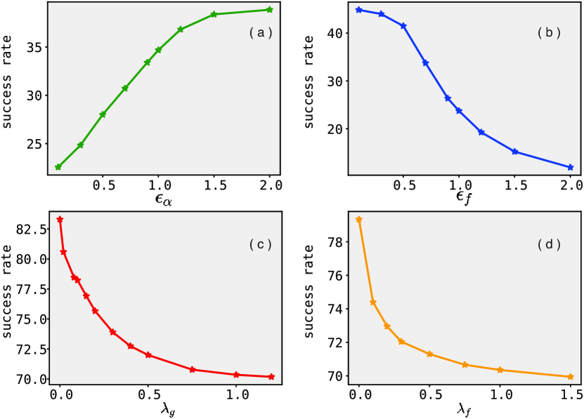
Figure 3: Influences of hyper-parameters. (a) and (b) shows success rate w.r.t. different upper bounds of $f$ (i.e., $\epsilon_{f}$) and $\alpha$ (i.e., $\epsilon_{\alpha}$) under the RI-AVA method. We also show the success rate w.r.t. different $\lambda_{g}$ and $\lambda_{f}$ in (c) and (d), respectively, under the RA-AVA method.

3.4 Geometry-aware Level-Set Optimization

To optimize Eq. (3.3), we first initialize the geometry vignetting, i.e., $\mathbf{G}=\mathbf{G}_{0}=1-\alpha\mathbf{R}$, which is a distance-related matrix and we reformulate it as a level-set function $\text{g}(u_{i},v_{i})=\mathbf{G}[i]=1-\alpha\sqrt{u_{i}^{2}+v_{i}^{2}}$. Intuitively, the function $\text{g}(\cdot)$ takes the coordinates of a position on the image plane as inputs and outputs a value that decreases as the coordinates become larger, leading to a 3D surface. With such a function, we can define the curve $\mathcal{C}$ as the $z$-level-set of $\text{g}(\cdot)$, i.e., $\mathcal{C}=\{(u_{i},v_{i})|z=\text{g}(u_{i},v_{i})\}$, that is, $\mathcal{C}$ is the cross section of the 3D surface at level $z$. Then, we can define the region inside the curve as $\Omega_{\text{in}}=\{(u_{i},v_{i})|z<\text{g}(u_{i},v_{i})\}$, which can be reformulated it as the function of g by the Heaviside function (i.e., $\text{H}(\cdot)$) Chan and Vese (2001), that is, we have $\Omega_{\text{in}}=\{(u_{i},v_{i})|\text{H}(g(u_{i},v_{i}))>z\}~{}\text{or}~{}\text{H}(\mathbf{G})$. Finally, we can reformulate Eq. (3.3) as

$$\arg\max_{\mathbf{G},\mathcal{P}}~{}J(\phi(\text{vig}(\mathbf{I},\mathcal{P}),y)-\lambda_{g}\|(\mathbf{G}-\mathbf{G}_{0})\odot\text{H}(\mathbf{G})\|^{2}_{2}$$

$$~{}~{}~{}+\lambda_{f}|f|_{2}-\lambda_{\alpha}|\alpha|_{2},\mathrm{~{}~{}subject~{}to~{}~{}}\forall\rho\in\mathcal{P},|\rho|_{\text{p}}\leq\epsilon_{\rho}.$$ (8)

Since the Heaviside function is differentiable we can optimize the objective function via gradient descent. Compared with Eq. (3.3), the proposed new formulation only contains two terms that should be optimized, i.e., $\mathbf{G}$ and $\mathcal{P}$, making the optimization more easier. In practice, we can calculate the gradient of $\mathbf{G}$ and $\mathcal{P}$ w.r.t. to the objective function and use the signed gradient descent to optimize $\mathbf{G}$ and $\mathcal{P}$ as is done in Kurakin et al. (2017).

3.5 Implementation Details

We show the whole process in Fig. 2(a). Specifically, given a clean image $\mathbf{I}$ and a DNN $\phi(\cdot)$, we summarize the workflow of our attacking algorithm in the following steps: ❶ Initialize the parameters $\mathcal{P}=\{f^{-1},\alpha,\tau,\chi\}=\{1,0,0,0\}$, the geometry vignetting matrix $\mathbf{G}$ as $1-\alpha\mathbf{R}$, and the distance matrix $\mathbf{R}$ via $\mathbf{R}[i]=\sqrt{u_{i}^{2}+v_{i}^{2}}$. ❷ Calculate the illumination-related matrix $\mathbf{A}$ via Eq. (2), and the camera tilting-related matrix $\mathbf{T}$ via Eq (4). ❸ At the $t$-th iteration, calculate the gradient of $\mathbf{G}_{t}$, $\mathcal{P}_{t}$ with respect to the objective function Eq. (3.4) and obtain $\nabla_{\mathbf{G}_{t}}$ and $\{\nabla_{\rho_{t}}|\rho_{t}\in\mathcal{P}_{t}\}$. ❹ Update $\nabla_{\mathbf{G}_{t}}$ and $\mathcal{P}_{t}$ with their own step sizes. ❺ Update $t=t+1$ and go to the step three for further optimization until it reaches the maximum iteration or $\text{vig}(\mathbf{I},\mathcal{P})$ fools the DNN. In the experimental parts, we set our hyper-parameters as follows: we set the stepsize of $f,\alpha,\tau,\chi$ and $\nabla_{\mathbf{G}_{t}}$ as 0.0125, 0.0125, 0.01, 0.01 and 0.0125, respectively. We set the number of iterations to be 40 and $z$ of the level-set method to be 1.0. We set ${p}$ to be $\infty$, and set the $\epsilon$ of $f^{-1}$, $\alpha$, $\tau$, and $\chi$ as 0.5, 0.5, $\pi/6$, and $\pi/6$. In addition, we set $\lambda_{f}$, $\lambda_{g}$ and $\lambda_{\alpha}$ all to be 1. In Section 4, we will carry out experiments to evaluate the effect of different hyper-parameters. And we do not choose the hyper-parameters for the highest success rate when compared with baseline attacks, but rather set the parameters that can balance the high success rate and good image quality.

4 Experimental Results

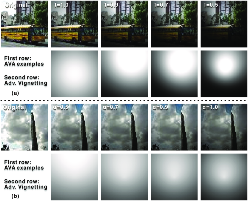
Figure 4: Visualization results of different ball bound for $f$ and $\alpha$.

	Crafted from	ResNet50			EfficientNet			DenseNet			MobileNet
	Succ Rate & Metrics	Succ Rate	BRISQUE	NIQE	Succ Rate	BRISQUE	NIQE	Succ Rate	BRISQUE	NIQE	Succ Rate	BRISQUE	NIQE
DEV	MIFGSM	99.78	20.93	39.42	99.89	19.12	39.38	100.00	21.17	40.19	100.00	22.79	42.19
	CW	100.00	17.49	48.36	100.00	17.81	48.36	100.00	17.48	48.53	100.00	17.33	48.51
	TIMIFGSM	96.23	18.34	45.86	98.56	18.59	46.15	98.34	18.48	45.60	98.94	18.55	45.99
	Wasserstein	14.21	20.91	51.63	32.78	20.44	51.30	16.50	20.67	51.79	13.87	20.02	51.58
	cAdv	81.59	18.44	51.48	88.27	18.45	51.38	77.85	18.43	51.46	78.73	18.44	51.36
	RI-AVA	9.36	19.78	48.33	14.95	20.06	48.24	13.07	20.10	48.17	20.68	20.32	48.12
	RA-AVA	96.77	21.33	46.92	98.34	22.81	47.02	99.22	20.89	46.54	99.18	21.20	46.66
CIFAR10	MIFGSM	80.78	41.86	42.04	96.67	41.90	42.53	79.03	41.40	41.97	97.87	41.56	42.14
	CW	100.00	41.43	41.36	100.00	41.66	41.06	100.00	41.34	41.42	100.00	41.46	41.01
	TIMIFGSM	38.80	41.66	40.64	38.64	41.54	40.59	34.82	41.48	40.62	59.77	41.44	40.67
	Wasserstein	80.27	45.45	44.47	74.73	44.81	44.09	80.62	43.26	42.05	66.43	43.45	42.87
	cAdv	12.78	41.42	40.78	21.24	41.55	40.78	11.88	41.32	40.84	17.28	41.40	40.84
	RI-AVA	6.17	40.54	40.28	9.53	39.90	40.34	6.73	40.57	40.28	12.52	39.73	40.36
	RA-AVA	35.95	33.56	38.05	74.15	28.29	35.39	45.80	31.48	37.39	84.66	24.82	35.63
Tiny ImageNet	MIFGSM	91.16	34.58	55.99	97.09	34.42	56.13	96.65	34.67	56.24	99.64	34.56	56.20
	CW	100.00	34.94	56.24	100.00	34.94	56.18	99.98	35.01	56.28	100.00	35.04	56.23
	TIMIFGSM	72.83	35.01	56.26	73.96	35.08	56.30	85.73	34.94	56.34	92.09	34.92	56.28
	Wasserstein	73.75	32.37	55.65	77.02	33.06	55.81	70.47	32.30	55.62	62.83	33.59	55.88
	cAdv	34.18	34.61	56.51	50.65	34.60	56.36	41.94	34.62	56.58	45.30	34.65	56.53
	RI-AVA	21.56	34.06	55.53	25.54	34.22	55.76	22.18	33.97	55.60	33.77	33.99	55.87
	RA-AVA	69.44	29.33	51.98	90.23	28.96	51.44	76.98	28.95	52.15	96.92	28.87	52.26

Table 1: Comparison results on 3 datasets with 5 attack baselines and our methods. It contains the success rates (%) of whitebox adversarial attack on three normally trained models: ResNet50, EfficientNet-b0, DenseNet121 and MobileNet-v2. The 1st column displays the whitebox attack results. The last two columns show the BRISQUE and NIQE score.

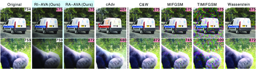
Figure 5: Adversarial examples generated with different methods. The top right corner shows the predictive label index and the ‘red’ numbers presents the attack misleads the DNN successfully. RI-AVA, RA-AVA, and cAdv are non-noise-based adversarial attack.

Here, we conduct comprehensive experiments on three popular datasets to evaluate the effectiveness of our method. We compare our method with some popular baselines including adversarial noise attack methods and other methods. Finally, we conduct experiments to showcase that our method can effectively defend against vignetting corrections.

Datasets. We carry out our experiments on three popular datasets, i.e., DEV Google (2017), CIFAR10 Krizhevsky et al. (2009), and Tiny ImageNet Stanford (2017).

Models. In order to show the effect of our attack method on different neural network models, we choose four popular models to attack, i.e., ResNet50 He et al. (2016), EfficientNet-B0 Tan and Le (2019), DenseNet121 Huang et al. (2017), and MobileNet-V2 Sandler et al. (2018). We train these models on the CIFAR10 and Tiny ImageNet dataset. For DEV dataset, we use the pretrained models.

Metrics. We choose attack success rate and image quality to evaluate the effectiveness of our method. The image quality measurement metrics are BRISQUE Mittal et al. (2012a) and NIQE Mittal et al. (2012b). BRISQUE and NIQE are two non-reference image quality assessment methods. A high score for BRISQUE or NIQE indicates poor image quality.

Baseline methods. We compare our method with five SOTA attack baselines, i.e., momentum iterative fast gradient sign method (MIFGSM) Dong et al. (2018), Carlini & Wagner L2 method (C&W${}_{\text{L2}}$) Carlini and Wagner (2017), translation-invariant momentum iterative fast gradient sign method (TIMIFGSM) Dong et al. (2019), Wasserstein attack via projected sinkhorn iterates (Wasserstein) Wong et al. (2019) and colorization attack (cAdv) Bhattad et al. (2019).

Analysis of physical parameters. Focal length and geometric factor are the two important parameters for the vignetting effect. We evaluate the influence of the two physical parameters by setting different norm ball constraint for $f^{-1}$, $\alpha$ via Eq (3.2). According to the result in Fig. 3(a) and (b), we observe that: ❶ Given different ball bound to $f$ and $\alpha$, the success rate of attack will be different. ❷ With the ball bound of $f$ growing, the success rate decreases. But as ball bound of $\alpha$ increases, the success rate increases. ❸ From the visualization results in Fig. 4, with the value of $f$ decreasing and the value of $\alpha$ increasing, the vignetting effect becomes more obvious. Therefore, we can conclude that a stronger vignetting effect can increase the attack success rate.

Analysis of different objective functions. We evaluate the effect of different energy terms by setting different coefficient values of energy terms, i.e., $\lambda_{g}$, $\lambda_{f}$ and $\lambda_{\alpha}$. From the result in Fig. 3(c)(d), we can see that: ❶ With the increasing of $\lambda_{g}$ and $\lambda_{f}$, the success rate of attack decreases accordingly. ❷ The restriction on the energy item will reduce the success rate, indicating that the energy item has certain constraints on the attack. In addition, we find that the change of $\lambda_{\alpha}$ almost does not affect the attack success rate, which shows that this energy item has minimal constraints on the attack.

	Crafted from	ResNet50					EfficientNet					DenseNet					MobileNet
	Attacked model & Metrics	EffNet	DenNet	MobNet	BRISQUE	NIQE	ResNet	DenNet	MobNet	BRISQUE	NIQE	ResNet	EffNet	MobNet	BRISQUE	NIQE	ResNet	EffNet	DenNet	BRISQUE	NIQE
DEV	MIFGSM	13.29	16.50	12.81	20.93	39.42	13.67	15.95	31.26	19.12	39.38	11.30	9.75	11.40	21.17	40.19	7.97	21.15	10.08	22.79	42.19
	CW	0.55	0.78	0.12	17.49	48.36	0.32	1.11	2.00	17.81	48.36	0.11	0.33	0.12	17.48	48.53	0.00	0.33	0.22	17.33	48.51
	TIMIFGSM	5.54	9.08	8.81	18.34	45.86	7.64	10.74	15.75	18.59	46.15	5.71	6.53	7.40	18.48	45.60	3.12	9.08	7.42	18.55	45.99
	Wasserstein	0.78	1.99	1.53	20.91	51.63	0.65	1.11	1.65	20.44	51.30	0.86	0.66	1.06	20.67	51.79	0.32	0.33	0.44	20.02	51.58
	cAdv	28.35	34.33	32.31	18.44	51.48	31.93	36.61	45.77	18.45	51.38	22.39	23.37	27.03	18.43	51.46	25.83	29.24	30.79	18.44	51.36
	RI-AVA	3.32	4.10	4.11	19.78	48.33	3.88	5.65	5.76	20.06	48.24	4.41	4.54	5.17	20.10	48.17	5.17	7.31	6.98	20.32	48.12
	RA-AVA	20.27	21.59	23.97	21.33	46.92	17.65	20.93	28.91	22.81	47.02	20.02	22.04	23.38	20.89	46.54	16.36	22.48	18.16	21.20	46.66
CIFAR10	MIFGSM	14.08	13.09	12.46	41.86	42.04	10.26	9.02	17.46	41.90	42.53	13.49	13.40	11.74	41.40	41.97	4.46	9.24	4.23	41.56	42.14
	CW	5.01	2.75	5.76	41.43	41.36	1.04	1.11	3.96	41.66	41.06	2.51	4.78	5.19	41.34	41.42	0.54	1.07	0.43	41.46	41.01
	TIMIFGSM	5.47	5.63	5.79	41.66	40.64	3.92	3.82	7.13	41.54	40.59	4.61	4.61	4.91	41.48	40.62	2.24	4.05	2.21	41.44	40.67
	Wasserstein	8.25	2.65	5.82	45.45	44.47	0.86	0.71	2.55	44.81	44.09	2.34	8.10	5.03	43.26	42.05	0.52	1.25	0.35	43.45	42.87
	cAdv	10.92	9.16	13.47	41.42	40.78	11.54	10.98	17.34	41.55	40.78	10.35	10.87	13.27	41.32	40.84	9.28	10.91	8.27	41.40	40.84
	RI-AVA	2.61	2.62	2.18	40.54	40.28	2.94	2.93	2.92	39.90	40.34	2.96	2.56	2.26	40.57	40.28	2.73	3.28	2.87	39.73	40.36
	RA-AVA	18.21	19.18	15.33	33.56	38.05	25.42	26.55	30.43	28.29	35.39	21.67	21.33	17.96	31.48	37.39	19.26	26.66	19.31	24.82	35.63
Tiny ImageNet	MIFGSM	18.71	22.81	17.19	34.58	55.99	13.37	15.48	23.30	34.42	56.13	17.74	18.43	15.73	34.67	56.24	5.10	9.61	5.40	34.56	56.20
	CW	5.24	4.90	5.87	34.94	56.24	2.07	2.07	5.83	34.94	56.18	2.48	3.30	3.83	35.01	56.28	0.45	0.90	0.38	35.04	56.23
	TIMIFGSM	10.44	15.06	11.76	35.01	56.26	7.66	9.89	14.88	35.08	56.30	10.34	10.22	10.99	34.94	56.34	4.33	6.45	4.97	34.92	56.28
	Wasserstein	5.81	4.97	7.75	32.37	55.65	2.13	2.37	5.99	33.06	55.81	2.94	3.84	5.22	32.30	55.62	0.70	0.92	0.63	33.59	55.88
	cAdv	28.24	29.53	34.57	34.61	56.51	31.40	32.93	42.37	34.60	56.36	27.04	28.19	34.51	34.62	56.58	25.13	28.12	26.31	34.65	56.53
	RI-AVA	7.02	8.10	6.98	34.06	55.53	6.63	6.78	8.87	34.22	55.76	7.87	7.16	6.44	33.97	55.60	6.28	8.44	5.85	33.99	55.87
	RA-AVA	30.45	32.42	29.72	29.33	51.98	27.41	28.20	37.61	28.96	51.44	29.49	29.98	29.53	28.95	52.15	19.56	25.68	19.82	28.87	52.26

Table 2: Adversarial comparison results on three datasets with five attack baselines and our methods. It contains the success rates (%) of transfer adversarial attack on three normally trained models: ResNet50 (ResNet), EfficientNet-b0 (EffNet), DenseNet121 (DenNet), and MobileNet-v2 (MobNet). The first three columns display the transfer attack results, where we use red, yellow, and blue to mark the first, second, and third highest success rate. And the last two columns show the BRISQUE score and NIQE score.

Comparison with baseline attacks. We evaluate the effectiveness of our attack with the baseline. Table 1 shows the quantitative results about the attack success rates and the image quality. We observe that for every dataset, RA-AVA reaches higher success rate than RI-AVA, indicating that tunable vignetting regions can greatly improve the success rate of attack. Compared with the noise-based adversarial attack, we found that our attack achieved lower success rate than MIFGSM, CW and TIMIFGSM attack. This is in line with our expectation since the image vignetting has more constraints on image perturbation than adding arbitrary noises. This is also why our method (RA-AVA) could have better image quality than the noise-based attack. We also noticed that on some models and datasets (e.g., DEV), RA-AVA could still achieve competitive results in terms of attack success rate while the image quality is better. Compared with the non-noise based attack, our method is better than cAdv significantly. Furthermore, we also find that our method can achieve much better transferability, which will be introduced later.

In Fig. 5, we have showcased some examples generated by baselines and our attack methods. The first column shows the original images while the following columns list the corresponding adversarial examples. It is clear that our method could generate high-quality adversarial examples that are smooth and realistic. However, we could find obvious noises in the examples generated by the adversarial noise attack methods, which are difficult to appear in the real world. For other non-noise attack methods, e.g., cAdv, they allow patterns that may appear in the real world but the change between the original and the generated image is very perceptible. Our method does not change the image too much while maintaining the realism in optical system for the vignetting effects.

Comparison on transferability. We then evaluate the transferability of different attacks. Table 2 shows the quantitative transfer attack results of our methods and the baseline methods. In transfer attack, one attacks the target DNN with the adversarial examples generated from other models. As we can see, in most cases, our method achieves much higher transfer success rate than others while the image quality is also higher. For example, the attack examples crafted from ResNet50 on DEV dataset achieves 37.21%, 40.75%, and 40.89% transfer success rate on EfficientNet, DenseNet, and MobileNet, with the lowest values of BRISQUE and NIQE, i.e., 11 and 37.04.

	ResNet50	EfficientNet	DenseNet	MobileNet
original	66.06	57.83	65.33	49.40
RA-AVA	19.72	4.47	14.60	0.71
zero-dce	29.40	12.96	24.81	10.24

Table 3: Accuracy of four models on Tiny Imagenet before attack, after RA-AVA attack and after Zero-DCE correction.

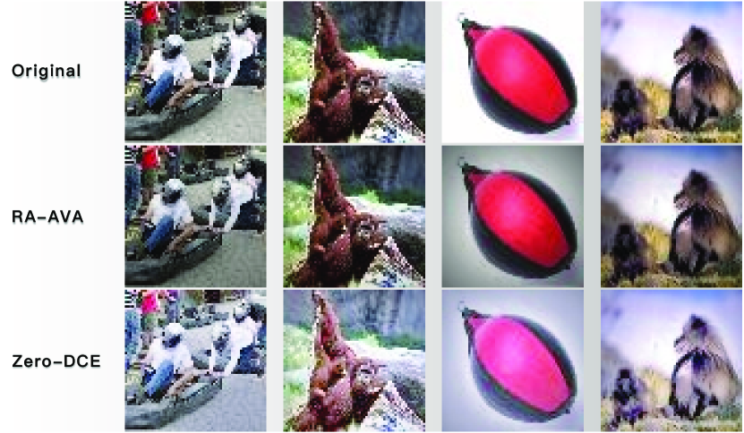
Figure 6: The visualization result of examples before attack, after RA-AVA attack and after Zero-DCE correction.

AVAs against vignetting corrections. Since our method is to use the vignetting effect as the attack method, we need to consider whether the method of light intensity and vignetting correction can neutralize our attack. For this reason, we use the Zero-DCE method Guo et al. (2020a) to adjust the light intensity. The visualization result is shown in Fig. 6. It can be seen that the Zero-DCE method has performed a certain brightness correction on the attacked images. The quantitative results of the accuracy change are shown in Table 3. After Zero-DCE correction, the accuracy has a certain improvement, but it is still lower than the original. It shows that the Zero-DCE method could mitigate the attack on some images but it is still not effective (e.g., only about 10% improvement), indicating that our attack method is robust against intensity and vignetting correction methods.

5 Conclusion

We have successfully embedded stealthy adversarial attack into the image vignetting effect through a novel adversarial attack method termed adversarial vignetting attack (AVA). By first mathematically and physically model the image vignetting effect, we have proposed the radial-isotropic adversarial vignetting attack (RI-AVA) and tuned the physical parameters such as the illumination factors and the focal length through the guidance of the target CNN models under attack. Next, by further allowing the effective regions of vignetting to be radial-anisotropic and shape-free, our proposed radial-anisotropic adversarial vignetting attack (RA-AVA) can reach much higher transferability across various CNN models. Moreover, level-set-based optimization is proposed to jointly solve the adversarial vignetting regions and physical parameters.

The proposed AVA-enabled adversarial examples can fool the SOTA CNNs with high success rate while remaining imperceptible to human. Through extensive experiments on three popular datasets and via attacking four SOTA CNNs, we have demonstrated the effectiveness of the proposed method over strong baselines. We hope that our study can mark one small step towards a fuller understanding of adversarial robustness of DNNs. In a long run, it can be important to explore the interplay between the proposed adversarial vignetting attack and other downstream perception tasks that are usually mission critical such as robust tracking Guo et al. (2020c); Cheng et al. (2021), robust autonomous driving Li et al. (2021), and robust DeepFake detection Qi et al. (2020); Juefei-Xu et al. (2021), etc.

Acknowledgement. This work has partially been sponsored by the National Science Foundation of China (No. 61872262). It was supported in part by Singapore National Cyber-security R&D Program No. NRF2018NCR-NCR005-0001, National Satellite of Excellence in Trustworthy Software System No. NRF2018NCR-NSOE003-0001, NRF Investigatorship No. NRFI06-2020-0022. We gratefully acknowledge the support of NVIDIA AI Tech Center (NVAITC) to our research.

References

- Asada et al. [1996] Naoki Asada, Akira Amano, and Masashi Baba. Photometric calibration of zoom lens systems. In ICPR, volume 1, pages 186–190. IEEE, 1996.
- Bhattad et al. [2019] Anand Bhattad, Min Jin Chong, Kaizhao Liang, Bo Li, and David A Forsyth. Unrestricted adversarial examples via semantic manipulation. arXiv preprint arXiv:1904.06347, 2019.
- Carlini and Wagner [2017] Nicholas Carlini and David Wagner. Towards evaluating the robustness of neural networks. In 2017 ieee symposium on security and privacy (sp), pages 39–57. IEEE, 2017.
- Chan and Vese [2001] T.F. Chan and L.A. Vese. Active contours without edges. IEEE TIP, 10(2):266–277, 2001.
- Cheng et al. [2020a] Yupeng Cheng, Qing Guo, Felix Juefei-Xu, Xiaofei Xie, Shang-Wei Lin, Weisi Lin, Wei Feng, and Yang Liu. Pasadena: Perceptually aware and stealthy adversarial denoise attack. arXiv preprint arXiv:2007.07097, 2020.
- Cheng et al. [2020b] Yupeng Cheng, Felix Juefei-Xu, Qing Guo, Huazhu Fu, Xiaofei Xie, Shang-Wei Lin, Weisi Lin, and Yang Liu. Adversarial exposure attack on diabetic retinopathy imagery. arXiv preprint arXiv:2009.09231, 2020.
- Cheng et al. [2021] Ziyi Cheng, Xuhong Ren, Felix Juefei-Xu, Wanli Xue, Qing Guo, Lei Ma, and Jianjun Zhao. Deepmix: Online auto data augmentation for robust visual object tracking. arXiv preprint arXiv:2104.11585, 2021.
- Croce and Hein [2019] Francesco Croce and Matthias Hein. Sparse and imperceivable adversarial attacks. In Proceedings of the IEEE International Conference on Computer Vision, pages 4724–4732, 2019.
- Dong et al. [2018] Yinpeng Dong, Fangzhou Liao, Tianyu Pang, Hang Su, Jun Zhu, Xiaolin Hu, and Jianguo Li. Boosting adversarial attacks with momentum. In Proceedings of the IEEE conference on computer vision and pattern recognition, pages 9185–9193, 2018.
- Dong et al. [2019] Yinpeng Dong, Tianyu Pang, Hang Su, and Jun Zhu. Evading defenses to transferable adversarial examples by translation-invariant attacks. In Proceedings of the IEEE Conference on Computer Vision and Pattern Recognition, pages 4312–4321, 2019.
- Gao et al. [2020] Ruijun Gao, Qing Guo, Felix Juefei-Xu, Hongkai Yu, Xuhong Ren, Wei Feng, and Song Wang. Making images undiscoverable from co-saliency detection. arXiv preprint arXiv:2009.09258, 2020.
- Gao et al. [2021] Ruijun Gao, Qing Guo, Felix Juefei-Xu, Hongkai Yu, and Wei Feng. Advhaze: Adversarial haze attack. arXiv preprint arXiv:2104.13673, 2021.
- Goldman [2010] Daniel B Goldman. Vignette and exposure calibration and compensation. IEEE TPAMI, 32(12):2276–2288, 2010.
- Gonzalez et al. [2004] Rafael C Gonzalez, Richard Eugene Woods, and Steven L Eddins. Digital image processing using MATLAB. Pearson Education India, 2004.
- Goodfellow et al. [2014] Ian J Goodfellow, Jonathon Shlens, and Christian Szegedy. Explaining and harnessing adversarial examples. arXiv preprint arXiv:1412.6572, 2014.
- Google [2017] Google. NIPS 2017: Adversarial Learning Development Set. https://www.kaggle.com/google-brain/nips-2017-adversarial-learning-development-set, 2017.
- Guo et al. [2018] Qing Guo, Shuifa Sun, Xuhong Ren, Fangmin Dong, Bruce Zhi Gao, and Wei Feng. Frequency-tuned active contour model. Neurocomputing, 275:2307–2316, 2018.
- Guo et al. [2020a] Chunle Guo, Chongyi Li, Jichang Guo, Chen Change Loy, Junhui Hou, Sam Kwong, and Runmin Cong. Zero-reference deep curve estimation for low-light image enhancement. In Proceedings of the IEEE/CVF Conference on Computer Vision and Pattern Recognition, pages 1780–1789, 2020.
- Guo et al. [2020b] Qing Guo, Felix Juefei-Xu, Xiaofei Xie, Lei Ma, Jian Wang, Bing Yu, Wei Feng, and Yang Liu. Watch out! Motion is Blurring the Vision of Your Deep Neural Networks. NeurPIS, 33, 2020.
- Guo et al. [2020c] Qing Guo, Xiaofei Xie, Felix Juefei-Xu, Lei Ma, Zhongguo Li, Wanli Xue, Wei Feng, and Yang Liu. Spark: Spatial-aware online incremental attack against visual tracking. In Proceedings of the European Conference on Computer Vision (ECCV), volume 2. Springer, 2020.
- He et al. [2016] Kaiming He, Xiangyu Zhang, Shaoqing Ren, and Jian Sun. Deep residual learning for image recognition. In Proceedings of the IEEE conference on computer vision and pattern recognition, pages 770–778, 2016.
- Huang et al. [2017] Gao Huang, Zhuang Liu, Laurens Van Der Maaten, and Kilian Q Weinberger. Densely connected convolutional networks. In Proceedings of the IEEE conference on computer vision and pattern recognition, pages 4700–4708, 2017.
- Juefei-Xu et al. [2021] Felix Juefei-Xu, Run Wang, Yihao Huang, Qing Guo, Lei Ma, and Yang Liu. Countering Malicious DeepFakes: Survey, Battleground, and Horizon. arXiv preprint arXiv:2103.00218, 2021.
- Kang and Weiss [2000] Sing Bing Kang and Richard Weiss. Can we calibrate a camera using an image of a flat, textureless lambertian surface? In ECCV, pages 640–653. Springer, 2000.
- Kass et al. [1988] Michael Kass, Andrew Witkin, and Demetri Terzopoulos. Snakes: Active contour models. International journal of computer vision, 1(4):321–331, 1988.
- Kimia et al. [1992] Benjamin B Kimia, Allen Tannenbaum, and Steven W Zucker. On the evolution of curves via a function of curvature. I. The classical case. Journal of Mathematical Analysis and Applications, 163(2):438–458, 1992.
- Krizhevsky et al. [2009] Alex Krizhevsky, Geoffrey Hinton, et al. Learning multiple layers of features from tiny images. 2009.
- Kurakin et al. [2016] Alexey Kurakin, Ian Goodfellow, and Samy Bengio. Adversarial machine learning at scale. arXiv preprint arXiv:1611.01236, 2016.
- Kurakin et al. [2017] Alexey Kurakin, Ian Goodfellow, and Samy Bengio. Adversarial examples in the physical world. ICLR (Workshop), 2017.
- Li et al. [2021] Yiming Li, Congcong Wen, Felix Juefei-Xu, and Chen Feng. Fooling lidar perception via adversarial trajectory perturbation. arXiv preprint arXiv:2103.15326, 2021.
- Mittal et al. [2012a] Anish Mittal, Anush Krishna Moorthy, and Alan Conrad Bovik. No-reference image quality assessment in the spatial domain. IEEE Transactions on image processing, 21(12):4695–4708, 2012.
- Mittal et al. [2012b] Anish Mittal, Rajiv Soundararajan, and Alan C Bovik. Making a “completely blind” image quality analyzer. IEEE Signal processing letters, 20(3):209–212, 2012.
- Qi et al. [2020] Hua Qi, Qing Guo, Felix Juefei-Xu, Xiaofei Xie, Lei Ma, Wei Feng, Yang Liu, and Jianjun Zhao. Deeprhythm: exposing deepfakes with attentional visual heartbeat rhythms. In Proceedings of the 28th ACM International Conference on Multimedia, pages 4318–4327, 2020.
- Ray [2002] Sidney Ray. Applied photographic optics. Routledge, 2002.
- Sandler et al. [2018] Mark Sandler, Andrew Howard, Menglong Zhu, Andrey Zhmoginov, and Liang-Chieh Chen. Mobilenetv2: Inverted residuals and linear bottlenecks. In Proceedings of the IEEE conference on computer vision and pattern recognition, pages 4510–4520, 2018.
- Stanford [2017] Stanford. Tiny ImageNet. https://www.kaggle.com/c/tiny-imagenet, 2017.
- Tan and Le [2019] Mingxing Tan and Quoc Le. Efficientnet: Rethinking model scaling for convolutional neural networks. In International Conference on Machine Learning, pages 6105–6114, 2019.
- Tian et al. [2020] Binyu Tian, Qing Guo, Felix Juefei-Xu, Wen Le Chan, Yupeng Cheng, Xiaohong Li, Xiaofei Xie, and Shengchao Qin. Bias field poses a threat to dnn-based x-ray recognition. arXiv preprint arXiv:2009.09247, 2020.
- Tsai [1987] Roger Tsai. A versatile camera calibration technique for high-accuracy 3d machine vision metrology using off-the-shelf tv cameras and lenses. IEEE Journal on Robotics and Automation, 3(4):323–344, 1987.
- Wang et al. [2020] Run Wang, Felix Juefei-Xu, Qing Guo, Yihao Huang, Xiaofei Xie, Lei Ma, and Yang Liu. Amora: Black-box adversarial morphing attack. In Proceedings of the 28th ACM International Conference on Multimedia, pages 1376–1385, 2020.
- Wong et al. [2019] Eric Wong, Frank R Schmidt, and J Zico Kolter. Wasserstein adversarial examples via projected sinkhorn iterations. arXiv preprint arXiv:1902.07906, 2019.
- Yu [2004] Wonpil Yu. Practical anti-vignetting methods for digital cameras. IEEE TCE, 50(4):975–983, 2004.
- Zhai et al. [2020] Liming Zhai, Felix Juefei-Xu, Qing Guo, Xiaofei Xie, Lei Ma, Wei Feng, Shengchao Qin, and Yang Liu. It’s raining cats or dogs? adversarial rain attack on dnn perception. arXiv preprint arXiv:2009.09205, 2020.
- Zheng et al. [2008] Yuanjie Zheng, Stephen Lin, Chandra Kambhamettu, Jingyi Yu, and Sing Bing Kang. Single-image vignetting correction. IEEE transactions on pattern analysis and machine intelligence, 31(12):2243–2256, 2008.