Abstract. Modeling extremes of climate variables in the framework of climate change is a particularly difficult task, since it implies taking into account spatio-temporal non-stationarities. In this paper, we propose a new method for estimating extreme precipitation at the points where we have not observations using information from marginal distributions and dependence structure. To reach this goal we combine two statistical approaches of extreme values theory allowing on the one hand to control temporal and spatial non-stationarities via a tail trend function with a spatio-temporal structure in the marginal distributions and by modeling on the other hand the dependence structure by a latent spatial process using generalized $\ell$-Pareto processes. This new methodology for trend analysis of extreme events is applied to rainfall data from Burkina Faso. We show that extreme precipitation is spatially and temporally correlated for distances of approximately 200 km. Locally, extreme rainfall has more of an upward than downward trend.

Keywords: Non-stationary POT, Generalized $\ell$-Pareto process, Space-time Extremes, Dependence Modeling, Trends detection, Climate Change.

1 Introduction

In the framework of climate change, the modeling and accurate prediction of the magnitude and extent of extreme events that occur in space and time of climate variables is a particularly difficult task, since it implies taking into account spatial and temporal non-stationarities. Nowadays there is a general consensus in the scientific community that climate change has accelerated in recent decades and that the climate will continue to change in the coming decades, mainly due to natural and anthropogenic changes (IPCC 2007, 2018,2019). This change is manifested in most regions of the world by a resurgence of heavy rainfall, heat waves and pollution peaks with very significant economic and social consequences. From a statistical point of view, the hypothesis of stationarity becomes untenable and debatable, and thus raises the question of detecting trends in extreme events, which has been the subject of much attention over the last 30 years. The classical Theory of Extreme Values extended both to non-stationary and non-independent observations provides a rigorous mathematical framework to deal with this question of trend detection in extremes ([13], [16], [19], [5]).

This issue was first generally studied in extreme value literature by parametric pointwise approaches in which an extreme value model (GEV or GPD) is fitted to the data at each site in turn, leaving the parameters of the marginal distributions to evolve with time or other significant covariates([8], [20], [21], [7], [24]). Although it is relatively simple to construct non-stationary models in the univariate framework, it is more difficult to account for spatial and temporal trends in these univariate models. The spatial and temporal dimension of extreme events was first developed for block maxima in a stationary framework and modeled by max-stable processes ([11], [17], [4], [3, 2]). These spatial models have been readapted to handle non-stationarities induced by global warming ([18], [6]). Although attractive, these models are expensive in computing time when tending towards large dimensions and are not adapted for modeling threshold exceedances.

The threshold exceedance approach introduced by [1] and [22] was first extended to multivariate environments ([23]) before being generalized to functional data ([15], [12], [9, 10]) to give birth to the family of generalized $\ell$-Pareto processes. This family of processes are better adapted to model the spatial dependence structure of exceedances data. However, these approaches do not sufficiently take into account marginal non-stationarities and spatial dependence between margins. In this paper we propose a new method to capture non-stationarities in marginal distributions, while taking into account the spatial dependence structure. To reach this goal we combine two statistical approaches of extreme value theory allowing on the one hand to control temporal and spatial non-stationarities via a tail trend function with a spatio-temporal structure in marginal distributions([13], [16], [5]) and by modeling on the other hand the dependence structure by a hidden stationary auxiliary process using generalized $\ell$-Pareto processes [10].

The article is organized as follows: section 2 provides a brief overview on generalized $\ell$-Pareto processes. Section 3 details the methodology implemented and the methods used to estimate the parameters. In section 4 we present our main results, and in particular we compare the stationary and non-stationary return levels computed from the developed approaches.

2 Overview on generalized $\ell$-Pareto process

Let $S$ be a compact subset of $\mathbb{R}^{d}$ and $T$ be a compact subset of $\mathbb{R}^{+}$ denoting the spatial and temporal domain respectively. We note by $\mathcal{C}(S)$ the set of continuous real functions on $S$ with the uniform norm $\parallel.\parallel_{\infty}$; $\mathcal{C}_{+}(S)$ its restriction to non-negative functions deprived of the null function and $\mathscr{M}\left\{\mathcal{C}_{+}(S)\right\}$ the class of measures associated with $\mathcal{C}_{+}(S)$.

Let $\left\{Z(s),s\in S\right\}$ be a latent spatial stochastic process indexed by $s\in S\subset\mathbb{R}^{d}$ with sample paths in $\mathcal{C}(S)$ of continuous marginal distribution $F_{Z}$ and common right endpoint $z_{F}$. As in ([15], [10]), we assume that the stationary process $Z$ is a general functional regular variation, noted $Z\in GRV(\gamma,a_{n},b_{n},\Lambda)$, i.e that there exists suitable sequences of continuous functions $a_{n}:S\longrightarrow\mathbb{R}^{+}$, $b_{n}:S\longrightarrow\mathbb{R}$ and $\gamma\in\mathbb{R}$ such that

$$nP\left[\left(1+\gamma\left((Z-b_{n})/a_{n}\right)\right)^{1/\gamma}_{+}\in.\right]\longrightarrow\Lambda(.),n\longrightarrow+\infty,$$ (1)

where $\Lambda$ is a non-zero measure in $\mathscr{M}\left\{\mathcal{C}_{+}(S)\right\}$ and homogeneous of order $-1$, with $\Lambda\left(tA\right)=t^{-1}\Lambda\left(A\right)$ for any positive real $t>0$ and Borel set $A\subset\mathcal{C}_{+}(S)$.

In the multivariate and spatial framework a threshold exceedances for a random function $Z=\left\{Z(s),s\in S\right\}$ is defined by Dombry and Ribatet [12] to be an event of the form $\left\{\ell(Z)>u\right\}$ for some $u\geq 0$, where $\ell:\mathcal{C}(S)\longrightarrow\mathbb{R}^{+}$ is a continuous and homogeneous non-negative risk function, i.e, there exists $\alpha>0$ such that $\ell(\lambda y)=\lambda^{\alpha}\ell(y)$ when $y\in\mathcal{C}_{+}(S)$ and $\lambda>0$. The risk function $\ell$ determines the type of extreme events of interest. For example, such a function can be the maximum, minimum, average or value at a specific point $s_{0}\in S$. Moreover, as in ([10], [14]) we assume that there exists a continuous and positive real function $A_{Z}$ such that the sequence $a_{n}$ and the risk function $\ell$ satisfy the following asymptotic decomposition

$$\begin{array}[]{c|c|c}\displaystyle\lim_{n\rightarrow\infty}\sup_{s\in\mathcal{S}}&\dfrac{a_{n}(s)}{\ell(a_{n})}-A_{Z}(s)&=0,~{}~{}~{}~{}\text{i.e}~{}~{}a_{n}(s)\approx\ell(a_{n})A_{Z}(s),~{}~{}n\rightarrow\infty\end{array}$$ (3)

The marginal distributions of $Z$ are supposed to belong to a location-scale family, thus ensuring a constant $\gamma\in\mathbb{R}$ shape parameter over any $S$, i.e. that there exist a $H$ distribution function such that

$$P\left(Z(s)\leq z\right)=H\left[\left(z(s)-B_{Z}(s)\right)/A_{Z}(s)\right],$$ (4)

where $A_{Z}:S\rightarrow\left(0;\infty\right[$ verifies asymptotic decomposition(3) and $B_{Z}:S\rightarrow\mathbb{R}$ are continuous functions. In particular $H$ must belong to the domain of attraction of a generalized extreme value (GEV) distribution of index $\gamma\in\mathbb{R}$, i.e., $F_{Z}\in\mathscr{D}(G_{\gamma})$. In other words, there are appropriate normalization real sequences $\tilde{a}_{n}>0$, $\tilde{b}_{n}\in\mathbb{R}$ such that $\displaystyle\lim_{n\rightarrow\infty}H^{n}\left(\tilde{a}_{n}z+\tilde{b}_{n}\right)=G_{\gamma}(z)$. The condition of the max-domain of attraction is equivalent to

$$\displaystyle\lim_{n\rightarrow+\infty}n\left[1-H\left(\tilde{a}_{n}z+\tilde{b}_{n}\right)\right]=-\log G_{\gamma}(z),~{}~{}z>0,$$ (5)

Under these conditions and the assumption of the general functional regular variation the suitable sequence of continuous functions $a_{n}(s)$ and $b_{n}(s)$, satisfy:

$$a_{n}(s)=\tilde{a}_{n}A_{Z}(s),~{}~{}~{}~{}~{}~{}b_{n}(s)=B_{Z}(s)+A_{Z}(s)\tilde{b}_{n},~{}~{}~{}~{}s\in S.$$ (6)

Functions $A_{Z}(s)$ and $B_{Z}(s)$ as well as the spatial dependence structure of $Z$ are assumed to belong to a family of parametric functions $\left\{A_{Z,\theta_{A}}:\theta_{A}\in\Theta_{A}\right\}$ ; $\left\{B_{Z,\theta_{B}}:\theta_{B}\in\Theta_{B}\right\}$ and $\left\{\Lambda_{\theta_{\Lambda}}:\theta_{\Lambda}\in\Theta_{\Lambda}\right\}$. Under minimal assumptions on the risk function and assumptions (1, 3) of $Z$, the conditional distribution of $\ell$-exceedance for some threshold $u\geq 0$ of the process $(Z-b_{n})/\ell(a_{n})$ can be approximated by a generalized $\ell$-Pareto process, for $n$ large enough([10])

$$\displaystyle P\left\{\Bigg{\lfloor}\dfrac{Z-b_{n}}{\ell\left(a_{n}\right)}\Bigg{\rfloor}\in A\mid\ell\left(\dfrac{Z-b_{n}}{\ell\left(a_{n}\right)}\right)\geq u\right\}\longrightarrow P\left\{W_{\ell}\in A\right\},n\longrightarrow\infty,$$ (7)

where $\lfloor z\rfloor=\max\left(z,A_{Z}\gamma^{-1}\right)$ if $\gamma>0$ and $\lfloor z\rfloor=z$ if $\gamma\leq 0$. $W_{\ell}$ is a non-degenerate stochastic process over S and belongs to the family of generalized $\ell$-Pareto processes with tail index $\gamma$, zero location, scaling function $A_{Z}$ and limit measure $\Lambda$. Specifically, a generalized $\ell$-Pareto process $W_{\ell}$ associated to the limit measure $\Lambda$ and tail index $\gamma\in\mathbb{R}$ is a stochastic process taking values in $\left\{z\in\mathcal{C}_{+}(S):\ell\left\{(z-b)/\ell(a)\right\}\geq 0\right\}$ and defined by:

$$W_{\ell}=\left\{\begin{array}[]{rl}a\left(Y_{\ell}^{\gamma}-1\right)/\gamma+b,~{}\gamma\neq 0\\ a\log Y_{\ell}+b,~{}~{}~{}~{}~{}~{}~{}~{}\gamma=0,\end{array}\right.;$$ (10)

where $a=\ell(a)A_{Z}>0$ and $b$ are continuous functions on $S$ respectively scale and location functions and $Y_{\ell}$ is a stochastic process whose probability measure is completely determined by the limit measure $\Lambda$. For the modelling of spatial dependence structure of latent process, we use $Y_{\ell}$ whose margins are in the Frechet max-domain of attraction with tail index $\gamma=1$, as the process of reference. A pseudo-polar decomposition of $Y_{\ell}$ in (10) leads to the following formulation ([12], [9])

$$Y_{\ell}=RQ$$ (11)

where $R$ is a unit Pareto random variable of index $\gamma_{R}$ representing the intensity of process, and $Q$ is stochastic process denoted the angular component with state space $S$ and taking values in $\mathscr{S}=\left\{y\in\mathcal{C}_{+}\left(S\right):\parallel y\parallel_{1}=1\right\}$ whose probability measure is characterized by limit measure $\Lambda$. More details on generalized $\ell$-Pareto processes can be found in ([15], [12], [9, 10]).

3 Space-time trends detection

Let $X=\left\{X_{t}(s),s\in S,t\in T\right\}$ be a continuous non-stationary space-time stochastic process with sample paths in the family of continuous functions $\mathcal{C}(S\times T)$ equipped with the uniform norm $\parallel.\parallel_{\infty}$, where $S\times T\subset\mathbb{R}^{d}\times\mathbb{R}^{+}$ and $\mathcal{C}_{+}(S\times T)$ its restriction to non-negative functions deprived of the null function. In practice $X$ is observed at each stations $s_{1},\cdots,s_{m}$ and at given dates $t=1,\cdots,n$. Let $F_{t,s}$ be the continuous univariate marginal distribution with a common right endpoint $x_{F}$ and $Z=\left\{Z(s),s\in S\right\}$ an unobserved latent spatial stochastic process with sample paths in $\mathcal{C}(S\times T)$ satisfying the properties described in the section (2) and the proportional tail condition such that

$$\displaystyle\lim_{x\rightarrow x_{F}}\dfrac{P\left(X_{t}(s)>x\right)}{P\left(Z(s)>x\right)}=c_{\theta}\left(\frac{t}{n},s\right),$$ (12)

where $c_{\theta}:\left[0,1\right]\times S\longrightarrow\left(0,\infty\right[$ is an assumed continuous and positive function depending on a parameter vector $\theta\in\Theta\subset\mathbb{R}$, called tail scale function or skedasis function ([13], [15, 16], [5]). In added we assume that the continuous marginal distributions $F_{Z}$ have a some common right endpoint as $F_{t,s}$. The skedasis function describes the evolution of extreme events jointly in space and time. The tail trend function $c_{\theta}$ is designed to ensure uniqueness of $c_{\theta}$ such that:

$$\dfrac{1}{m}\sum_{j=1}^{m}\int_{0}^{1}c_{\theta}\left(u,s_{j}\right)du=1,~{}~{}u\in\left[0,1\right],~{}~{}s_{j}\in S.$$ (13)

In the framework of the model (12), Mefleh et al.[19] shows that the empirical point measure converges in distribution in the space of point measure $\mathcal{M}_{p}=\mathcal{M}_{p}\left([0,1]\times(0,\infty]\right)$ to a Poisson point process with intensity measure $c(u)du\gamma z^{-(\gamma+1)}dz$ on $[0,1]\times(0,\infty]$. In such a case the times of exceedances for high threshold $x$ and the value of exceedances are asymptotically independent with distributions respectively equal to the trend density function $c_{\theta}(u,s),s\in S$ and the Pareto distribution of tail index $\gamma$. Several models are eligible to model the function $c_{\theta}$, but in this study we opt for parametric models because of their flexibility in trend detection and in order to make extrapolations of the trend beyond the observed data. We are interested in monotonic log-linear and simple linear trend models of $c_{\theta}$. We introduce a spatial structure in the tail function by letting the parameter $\theta$ evolve as a function of geographic coordinates (longitude, latitude), that is,

$$\left\{\begin{array}[]{rl}c_{\theta}^{1}(\frac{t}{n},s)=\dfrac{\theta(s)}{\exp\{\theta(s)\}-1}\exp\{\theta(s)\frac{t}{n}\},~{}~{}\theta(s)\in\mathbb{R};~{}\frac{t}{n}\in\left[0,1\right]\\ \\ c_{\theta}^{2}(\frac{t}{n},s)=\theta(s)\left\{2\frac{t}{n}-1\right\}+1,~{}~{}\theta(s)\in\left]-1;1\right[;~{}~{}\frac{t}{n}\in\left[0,1\right]\end{array}\right.;$$ (17)

where $\theta(s)=\theta_{0}+\sum_{k=1}^{2}\theta_{k}Y_{k}(s)$ with $(Y_{1},Y_{2})=(Long,Lat)$. The parameter vector $\theta=\left(\theta_{0},\theta_{1},\theta_{2}\right)$ is then estimated using the maximum likelihood method and multiple linear regression.

3.1 Marginal model of latent process

The marginal parameters $\gamma$, $a_{n}$, $A_{Z}$, $b_{n}$ and $B_{Z}$ of the latent spatial process $Z$ are estimated under the constraint that $u_{n}=\ell(b_{n})+u\ell(a_{n})$, following the modeling assumptions described in section(2). For simplicity purpose we choose $u=0$ so that $\ell$-exceedances of $Z$ are defined as events for which $\ell(Z)\geq\ell(b_{n})$. In this case a natural choice of $u_{n}=\ell(b_{n})$ is a high quantile of the variable $\ell(Z)$, for example $u_{n}=q_{0.95}\left\{\ell\left(Z\right)\right\}$. In general, a parametric model may be necessary for $a_{n}$ and $b_{n}$, as in Engelke et al.[14], but we consider in this work that $a_{n}(s_{j})=a_{j}>0$ and $b_{n}(s_{j})=b_{j}\in\mathbb{R}$ for any $j=1,\cdots,m$. The threshold stability of the generalized Pareto distributions does not allow us to identify the $b_{n}$ function without additional assumptions, so under the assumption that $\ell(B_{Z})=0$, we set

$$b_{n}(s)=u_{q^{\prime}}\left\{Z(s)\right\}-\tilde{b}_{n},~{}~{}~{}s\in S,$$ (18)

where $\tilde{b}_{n}=\ell(b_{n})=u_{n}$ (see 3 and 6) and $u_{q^{\prime}}\left\{Z(s)\right\}$ is an empirical quantile of the order $q^{\prime}$ of the $\ell$-exceedances at each location $s$, where $q^{\prime}$ is chosen such that $\ell(b_{n})=\tilde{b}_{n}$ in order to impose the identifiability of the parameters. Thus, the tail index $\gamma\in\mathbb{R}$ and the scale parameters $a_{n}(s)>0$ are estimated by maximizing the independent log-likelihood; that is

$$\ell_{indep}(\gamma,a_{n}(s_{j}))=\displaystyle\sum_{t=1}^{n}\sum_{j=1}^{m}\mathbb{1}_{\left\{x_{t}(s_{j})\geq b_{n}(s_{j})\right\}}\log\left[\dfrac{1}{a_{n}(s_{j})}\left\{1+\gamma\dfrac{x_{t}(s_{j})-b_{n}(s_{j})}{a_{n}(s_{j})}\right\}^{-1/\gamma-1}_{+}\right]$$ (19)

The estimate of parameters $A_{Z}$ and $B_{Z}$ are deducted from (6) under the assumptions of parameter identifiability, i.e, $\ell(A_{Z})=1$ and $\ell(B_{Z})=0$, which implies that $\ell(a_{n})=\tilde{a}_{n}$. Thanks to the equation(12) and the convergence of $Z$ exceedances to a GPD distribution we deduce a sample of $\left\{Z_{t}(s)\right\}$ from observations of $\left\{X_{t}(s)\right\}$ ([16] and [5]) in the following manner:

$$\widehat{Z}_{t}(s)=\left\{\widehat{c}_{\theta}\left(\frac{t}{n},s\right)\right\}^{-\widehat{\gamma}}\left[X_{t}\left(s\right)-\frac{\left\{\widehat{c}_{\theta}\left(\frac{t}{n},s\right)\right\}^{\widehat{\gamma}}-1}{\widehat{\gamma}}\left(\widehat{\tilde{a}}_{n}-\widehat{\gamma}\widehat{\tilde{b}}_{n}\right)\right],$$ (20)

where $\widehat{\gamma},\widehat{\tilde{a}}_{n},\widehat{\tilde{b}}_{n}$ and $\widehat{c}_{\theta}$ are respectively consistent estimators of $\gamma,\tilde{a}_{n},\tilde{b}_{n}$ and $c_{\theta}$ described in section (3.1).

3.2 Spatial extremal dependence

After removing the non-stationarity the modeling is focused on the evaluation of the remaining extreme spatial dependence structure in $Z$. Thus we approach the limit distribution of $\ell$-exceedances of $Z$ by a generalized $\ell$-Pareto process [10]. In the framework of the Brown-Resnick model, the angular component of $Q$ is a log-Gaussian random function whose underlying Gaussian process has stationary increments, which allows in particular to use classical dependence structures from the geostatistical literature to characterize the spatial dependence. In order to better capture this dependence structure, we use a flexible parametric semi-variogram belonging to the class of power semi-variograms. We estimate the parameter vector $\theta_{\Lambda}$ of the dependence structure using the gradient score method or the censored likelihood method [9].

3.3 Non-stationary return period and return level

The concept of return period and level becomes very ambiguous when we leave the stationary context to the non-stationary framework. In this paper, we have chosen to follow return period based approaches,i.e., Expected Number of Exceedances(ENE) [21] and Expected Waiting Time (EWT) ([20], [7]). In the ENE approach, the number of times the variable $X_{t}(s),s\in S$ exceeds the return level value $x_{m}$ in $m$ years is defined by $N_{m}=\sum_{t=1}^{n_{x}m}\mathbb{1}_{\left\{X_{t}(s)>x_{m},s\in S\right\}}$ under non stationary context. The return level $x_{m}$ can be defined as the value for which the expected number of events exceeding $x_{m}$ in $m$ years equals to one, i.e., the return level $x_{m}$ is the solution of the following equation:

$$\displaystyle 1=\sum_{t=1}^{n_{x}m}\left\{1-F_{t,s}\left(x_{m}\mid\theta_{t}(s)\right)\right\},~{}~{}s\in S,$$ (21)

where $n_{x}$ is the number of days in the year and $\theta_{t}(s)$ the vector of time-dependent marginal parameters or other covariates. Parey et al.[21] uses the ENE method in a pointwise POT model where the parameters of the distribution of exceedances and the intensity of extreme event occurrences are described as polynomial functions of time.

The EWT method was first proposed by Olsen et al.[20], and then derived by Salas and Obeysekera [24] using a geometric distribution with time-varying parameters. Under non stationary conditions, the distribution describing waiting time $Y$ before the first occurrence of an event exceeding the return level $x_{m}$ is

$$f_{s}(y)=P\left(Y(s)=y\right)=p_{y,s}\prod_{i=1}^{y-1}\left(1-p_{i,s}\right),y=1,2,\cdots,y_{\max}~{}~{}\text{and}~{}s\in S,$$ (22)

where variable $Y$ is the day of the first occurrence of an event exceeding the quantile $x_{m}$ , $p_{t,s}=1-F_{t,s}(x_{m}\mid\theta_{t}(s))$ is daily exceedance probability varying with time step t. $y_{\max}$ is the time when the daily exceedance probability $p_{t,s}$ is equal to 1 for an increasing-trend series or is equal to 0 for a decreasing-trend series. Reused and simplified by [7], the EWT approach defines the $m$-year return level $x_{m}$, as the value for which the expected waiting time until an exceedance of this level is $m$ years, i.e, $x_{m}$ is the solution of the equation:

$$n_{x}m=E\left[Y\right]=1+\displaystyle\sum_{y=1}^{\infty}\prod_{t=1}^{y}F_{t,s}\left(x_{m}\mid\theta_{t}(s)\right),s\in S.$$ (23)

Using the relationship (12), $P(X_{t}(s)>x_{m})$ can be rewritten $c_{\theta}(\dfrac{t}{n},s)P(Z(s)>u)P(Z(s)>x_{m}\mid Z(s)>u)$ for $u<x_{m}$ and we obtain the following results

Proposition 3.1

Let $\{X_{t}(s),s\in S,t\in T\}$ be a non-stationary stochastic process defined on a region $S\subset\mathbb{R}^{d}$ and $\{Z(s),s\in S\}$ a latent spatial process satisfying the equation 12. Given a return period $m$ and threshold $u<x_{m}$, the return level $x_{m}$ for all $s\in S$ is a solution of the following two equations:

1. Return period as expected number of events

   $$1=\displaystyle\sum_{t=t_{0}}^{t_{0}+n_{x}m}\left\{c_{\theta}\left(\frac{t}{n},s\right)\phi_{u}(s)\bar{F}_{Z,s}(x_{m}-u)\right\},$$ (24)

2. Return period as expected waiting time

   $$n_{x}m=1+\displaystyle\sum_{i=1}^{\infty}\prod_{t=1}^{i}\left\{1-c_{\theta}(\dfrac{t}{n},s)\phi_{u}(s)\bar{F}_{Z,s}(x_{m}-u)\right\},$$ (25)

where $\bar{F}_{Z,s}$ is a survival of generalized Pareto distribution of $\ell$-exceedances at position $s$; $\phi_{u}(s)=P(Z(s)>u)$ is the probability of exceedances, $c_{\theta}$ is the tail trend function and $n_{x}$ is the number of days in the year.

The return levels derived from the equations (24 & 25) are evaluated by numerical algorithms taking into account the information from the extrapolation of the trend function $c_{\theta}$ on the one hand and the spatial dependence structure of the latent stationary process $Z$ on the other hand. To derive the return level at points where we have not observations, we assume, the spatial process $Z$ is locally stationary in space. Under these new assumptions and using the knowledge of the spatial dependence structure of the latent process $Z$ and the equation(20), we propose the following result:

Proposition 3.2

Let $\{X_{t}(s),s\in S,t\in T\}$ be a non-stationary spatio-temporal stochastic process defined on a region $S\subset\mathbb{R}^{d}$ and $\{Z(s),s\in S\}$ a latent spatial process. The non-stationary return level $x_{m}(s),s\in S$ of the non-stationary process $X$ is deduced from the return level $z_{m}$ of the latent spatial process $Z$ such that:

$$x_{m}(s)=z_{m}(s)\widehat{c}_{\theta}(t_{m},s)^{\widehat{\gamma}}+\dfrac{\widehat{c}_{\theta}(t_{m},s)^{\widehat{\gamma}}-1}{\widehat{\gamma}}\left(\widehat{\tilde{a}}_{n}-\widehat{\gamma}\widehat{\tilde{b}}_{n}\right),~{}~{}s\in S,$$ (26)

where $\widehat{\tilde{a}}_{n}$, $\widehat{\tilde{b}}_{n}$ $\widehat{c}_{\theta}$ and $\widehat{\gamma}$ are the respective estimators of $\tilde{a}_{n}$, $\tilde{b}_{n}$, $c_{\theta}$ and $\gamma$. $t_{m}=1+\dfrac{n_{x}m}{n}$ with $n_{x}$ the number of days in the year and n the size of the sample observed.

This result is a consequence of the equation (20) and will be used to derive the non-stationary return levels of process $X$, using the $z_{m}$ computed from the estimated parameters. Thus, to calculate the $z_{m}$ at grid points where we have not observations, we use a spatial model from marginal parameters to build a spatial map on the domain of study based on covariates such as longitude and latitude.

4 Application to extreme precipitation in Burkina Faso

4.1 Data set analysis

This study uses time series of daily precipitation measurements from 1957 to 2016 provided by ten synoptic stations extracted from the Burkina Faso climatological database. These stations have been selected to ensure good spatial uniformity and representativeness of different climatic regimes and data quality. The figure1 gives the spatial distribution of the synoptic stations in our study area. In order to limit the problems related to seasonal rainfall cycles on each station, we worked from the sub-series corresponding to rainy days. The period from may to october was chosen because during this period that the most rainfall is recorded in Burkina Faso. Thus, a serie of 60 by 184 days is extracted to constitute the time series of daily rainfall. On these time series, we apply a run declustering procedure with a daily step (r=1 day) to identify the groups of approximately independent extreme observations within the sample in order to avoid short-term dependencies in the time series.

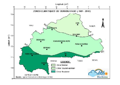
Figure 1: Spatial distribution of synoptic sampling stations associated with climatic regimes, source: National Meteorology Agency of Burkina Faso.

4.2 Marginal characteristics

The scale $a_{n}(s)$, location $b_{n}(s)$ and parameters of log-linear and linear trend function $c_{\theta}$ are estimated for any $s\in S$ and are shown respectively on maps (a), (b), (c) and (d) of figure(2).

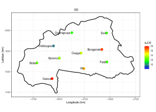
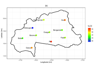
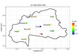
Figure 2: Estimated functions $a_{n}$ (2a) and $b_{n}$ (2b) of the generalized $\ell$-Pareto process for modelling extreme precipitation in Burkina Faso, and $\theta$ for Log-linear (2c) and simple linear(2d) trends. Estimates are obtained by shifting the local empirical quantiles $u_{0.95}\left\{Z(s)\right\}$ by $\widehat{\tilde{b}}_{n}=56.1mm$.

In practice we deduce from the generalized $\ell$-Pareto model fitted to the data, the marginal tail behavior of the survival distribution $\bar{F}_{Z,\widehat{\gamma}(s),\widehat{\sigma}(s)}$ for any $s\in S$ from the equation (27) given a sufficiently large $u_{q}>0$ threshold.

$$P\left[Z(s)-u_{q}(s)\geq z\mid Z(s)\geq u_{q}(s)\right]\approx\bar{F}_{Z,\widehat{\gamma}(s),\widehat{\sigma}(s)}(z),~{}~{}z\geq 0,$$ (27)

with $\widehat{\sigma}(s)=\widehat{a}_{n}(s)+\widehat{\gamma}\left(u_{q}(s)-\widehat{b}_{n}(s)\right)$, $s\in S$, where $\widehat{a}_{n}$, $\widehat{b}_{n}$, and $\widehat{\gamma}$ are the marginal parameters estimators described in section (3.1). We can use it to check the quality of the marginal adjustment of the stationary process $Z$. Figure 3 shows the QQplots of the local tail distribution due to two stations by climatic zone. Columns 1, 2, and 3 of Figure 3 represent the respective adjustments for the Sudanian, Sudano-Sahelian, and Sahelian zones. Globally, the fit of the marginal models seems convincing, as most of the observations remain within the confidence intervals.

Sudanian climate	Sudano-Sahelian climate	Sahelian climate

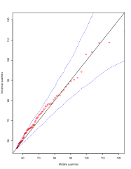
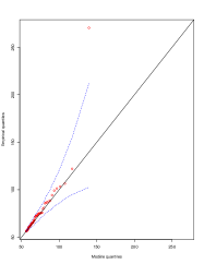
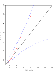
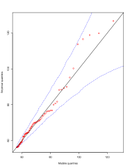
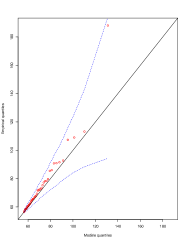
Figure 3: QQplot of local tail distributions of six synoptic positions. The thresholds correspond to the local 0.865 quantiles of the $\ell$-exceedances.

Furthermore, the sign of the $\theta$ parameter of the trend function tells us that the frequencies of extreme precipitation are locally quite variable throughout the study region. They have an increasing trend ($\theta>0$) in areas such as Ouahigouya, Bogande, Boromo, Gaoua, and Po. On the other hand, at the Ouagadougou and Fada stations, extreme rainfall frequencies tend to decrease ($\theta<0$). Figure 4 gives us the details of the adjustment of the tail trend function by a log-linear model.

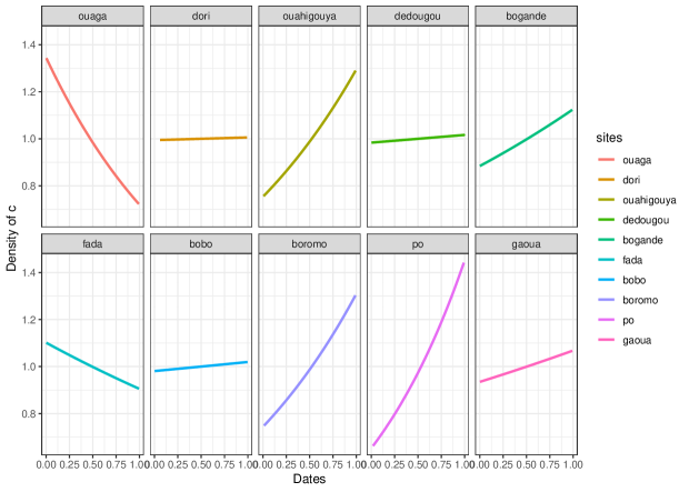
Figure 4: Local adjustment of evolution of the frequencies of extreme precipitation by a log-linear model trend $c_{\theta}^{1}$.

4.3 Estimated spatial dependence model

We use a spatial model of the marginal parameters dependent on significant covariates to obtain the marginal parameters at the different grid points using a generalized linear regression model, in order to prepare the ground for calculations of non-stationary return levels at locations where we have no observations.

$$\left\{\begin{array}[]{rl}a_{n}(s)=a_{0}+a_{1}Long\times Lat(s){}{}{}{}{}{}{}{}{}{}{}{}{}{}{}\\ b_{n}(s)=b_{0}+b_{1}Lat^{2}(s)+b_{2}Long\times Lat(s)\\ \theta(s)=\theta_{0}+\theta_{1}\times Long+\theta_{2}Lat{}{}{}{}{}{}{}{}{}{}{}{}{}{}\\ \gamma(s)=\gamma_{0}\par\par{}{}{}{}{}{}{}{}{}{}{}{}{}{}{}{}{}{}{}{}{}{}{}{}{}{}{}{}{}{}{}{}{}{}{}{}{}{}{}{}{}{}\end{array}\right.,~{}~{}s\in\mathcal{N}_{s_{0}},$$ (32)

where $\mathcal{N}_{s_{0}}$ is a small neighborhood around $s_{0}$. In what follows, these regional neighborhoods will be determined by a small number, $D_{0}$ of nearest stations from the site $s_{0}$, thus we will write $\mathcal{N}_{s_{0}}=\mathcal{N}_{s_{0},D_{0}}$ . Obviously, the choice of neighbourhood is important; the assumed stationary marginal parameters could be a poor approximation for large neighbourhoods (i.e., for large $D_{0}$ ), while the simulation of the process could be cumbersome for small neighbourhoods characterized by a small $D_{0}$ number of stations. In principle, the choice of $D_{0}$ should be such that the spatial dependence structure and marginal parameters is approximately stationary within each selected neighborhood $\mathcal{N}_{s_{0},D_{0}}$ around $s_{0}\in\mathcal{G}$. We obtain the relatively homogeneous, non-overlapping sub-regions using the k-means clustering method centered on the reference stations. This method is extensively used because it is computationally simple and produces accurate results, compared to other more complex clustering methods. The longitude and latitude of the grid points were used as input variables in the k-means clustering algorithm to form the ten clusters centered on the reference stations.

In addition, to better take into account the dependence structure of precipitation data and capture the possible isotropic, we choose a flexible parametric semi-variogram $\nu$ belonging to the power class models such that $\nu(h)=\left(\|h\|/\tau\right)^{\kappa}$, with $\tau>0$, $h\in\mathbb{R}^{2}$, $\kappa\in\left]0,2\right]$. We check the adequacy of the fit of the model to the data using the extremogram and the variogram. Figures (5a) and (5b) show respectively the good quality of the fit of the dependence measures such as the semi-variogram and extremogram. In Figure(5a), the points in gray represent the calculated empirical extremogram and the blue curve is the fitted empirical extremogram, while the red curve represents our fitted dependence model. The red curve in Figure 5b is the variogram model fitted to the data as a function of distance.

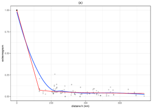
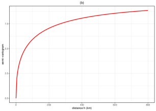
Figure 5: Isotropic extremogram $\pi(h)=\displaystyle\lim_{q\rightarrow 1}P(Z(s+h)>u_{q}(s+h)\mid\{Z(s)>u_{q}(s),\ell(Z)>u\}$ (Figure 5a) and variogram (Figure 5b) estimated for risk functional $\ell(Z)=\max_{s\in S}Z(s)$ of distance between locations $s$ and $s+h$.

It is noted that extreme precipitation is spatially correlated for distances of the order of 200km. This spatial dependence decreases gradually as the distance increases before stabilizing for example for a value of $\pi(h)=0.0625$. This reflects the very localized nature of extreme rainfall and it comforts us in our analysis because this property is generally present in rainfall data.

4.4 Non-stationary return level results

The return levels $x_{50}$ and $x_{100}$ are first estimated punctually (see Figure7) using the equations (24 & 25) before being spatially interpolated to the points where we have no observations using the dependence structure estimated from the observed data and parameters of trend function spatially extrapolated to the section (4.3).

Sudanian climate	Sudano-Sahelian climate	Sahelian climate

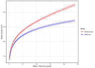
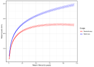
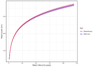
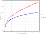
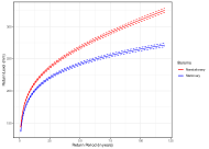
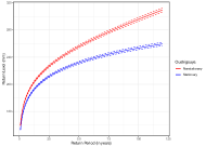
Figure 6: Trends of stationary and non-stationary return levels at reference stations computed with a log-linear tail trend function.

For a given return period $m$, we first compute the return levels $z_{m}$ on each point of grid from the latent spatial process $Z$ using the estimated spatial model, before deriving the non-stationary return levels $x_{m}$ using the equation 26 of proposition 3.2. We repeat this operation for different values of the return period $m$ and we deduce on each point of the grid, the associated return level (Figure 6). We can then produce maps of the return levels obtained from the dependence structure and the extrapolation of the trend function for a future period $m$. Thus, the extreme precipitation likely to be observed on average at least once every 50 years (resp. 100 years), will be particularly intense in the Sudanian and Sudano-Sahelian zone and less intense in the Sahelian zone, with a potentially quite strong spatial dependence within a radius of 200 km. The southwest and eastern regions of the country will be most affected by extreme precipitations. The results of the return level for a return period $m=50$ and $100$ years are displayed in Figures (7).

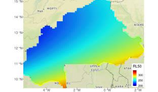
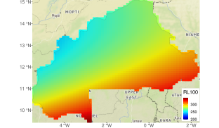
Figure 7: Maps of the non-stationary 50-years return levels(left) and 100-years return level (right) obtained by extrapolating the information from the log-linear tail trend function and the dependence structure.

5 Conclusion

In this study we proposed a new flexible methodology for trend detection in the extremes capable of capturing marginal non-stationarities and the dependence structure between margins using generalized $\ell$-Pareto processes. We computed the non-stationary return levels of rainfall in Burkina Faso at points where we have no observations and we showed that these extreme rainfall events are spatially correlated around a radius of 200km. This spatial dependence decreases progressively as the distance increases. In sum, we set up a non-stationary stochastic generator of extreme rainfall in Burkina Faso.

Appendix A Proof of proposition 3.1

1. Proof.Let $N_{m}$ be a random variable describing the number of exceedances for a period of time $m$; it comes that

   $$N_{m}=\displaystyle\sum_{t=t_{0}}^{to+n_{x}m}\mathbb{1}_{\left\{X_{t}(s)>x_{m}(s)\right\}}\Rightarrow E\left[N_{m}\right]=\sum_{t=t_{0}}^{t_{0}+n_{x}m}E\left(\mathbb{1}_{\left\{X_{t}(s)>x_{m}(s))\right\}}\right).$$

   And according to the equation (12), we have

   $$E\left[N_{m}\right]=\sum_{t=t_{0}}^{t_{0}+n_{x}m}P\left(X_{t}(s)>x_{m}(s)\right)=\sum_{t=t_{0}}^{t_{0}+n_{x}m}c_{\theta}\left(\frac{t}{n},s\right)P\left(Z_{t}(s)>x_{m}(s)\right).$$

   Moreover, given a sufficiently large $u(s)$ threshold with $s\in S$,

   $$P\left[Z_{t}(s)>x_{m}(s)\right] = P\left[Z_{t}(s)>u(s)\right]*P\left[Z_{t}(s)-u(s)>x_{m}(s)\mid Z_{t}(s)>u(s)\right]$$

   $$\approx \phi_{u}(s)*\bar{F}_{Z}\left[x_{m}(s)-u(s),\sigma(s),\gamma(s)\right],x_{m}(s)>u(s)$$

   Furthermore, it follows that

   $$E\left[N_{m}\right]=1 \Rightarrow \displaystyle\sum_{t=t_{0}}^{t_{0}+n_{x}m}\left\{c_{\theta}\left(\frac{t}{n},s\right)\phi_{u}(s)*F_{Z}\left(x_{m}(s)-u(s),\sigma(s),\gamma(s)\right)\right\}=1$$

   Which gives

   $$\displaystyle\sum_{t=t_{0}}^{t_{0}+n_{x}m}\left\{\phi_{u}(s)c_{\theta}\left(\frac{t}{n},s\right)\left(1+\frac{\gamma(s)}{\sigma(s)}\{x_{m}(s)-u(s)\}\right)^{-1/\gamma(s)}\right\}=1$$

   with $\sigma(s)=a_{n}(s)+\gamma(s)(u(s)-b_{n}(s))$

2. The result (25) is shown in a similar way   

Appendix B Asymptotic distribution of $\ell$-Pareto Process

For a threshold vector $u=(u_{1},\cdots,u_{d})\in\mathbb{R}^{d}_{+}$ and for any regularly varying stochastic process $Z\in GRV\left\{\gamma,a_{n},b_{n},\Lambda\right\}$, the density function of the $\ell$-excess of a $\ell$-Pareto process is obtained by renormalizing suitably the intensity function $\lambda$ found by taking the partial derivatives of the previously defined measure $\Lambda$ (1) by $\Lambda\left(A_{\ell}(u)\right)$:

$$f_{\ell,u}(z)=\dfrac{\lambda(z)}{\Lambda\left\{A_{\ell}(u)\right\}},~{}~{}z\in A_{\ell}(u),$$ (33)

where

$$\Lambda\left\{A_{\ell}(u)\right\}=\int_{A_{\ell}(u)}\lambda(z)dz,$$

while $\lambda$ is the intensity function and $A_{\ell}(u)=\left\{z\in\mathbb{R}_{+}^{d}:\ell\left(z/u\right)\geq 1\right\}$ the region of exceedances. In order to make inferences and to model the dependence structure of $\ell$-Pareto processes, we focus on the Brown-Resnick model for which the formulas of $\Lambda$ and $\lambda$ are available. The $d$-dimensional intensity function of the Brown-Resnick model is given:

$$\lambda_{BR}(z)=\dfrac{\mid\Sigma\mid^{-1/2}}{z_{1}^{2}z_{2},\cdots,z_{d}\left(2\pi\right)^{(d-1)/2}}\exp\left(-\frac{1}{2}\bar{z}^{T}\Sigma^{-1}\bar{z}\right),~{}~{}z\in\mathbb{R}^{d}_{+}$$

where $\bar{z}_{i}=\log\frac{z_{i}}{z_{1}}+\gamma(s_{i}-s_{1})$ and $\Sigma$ the covariance matrix.

To better capture the possible dependence structure we use anisotropic semi-variograms whose parameters change with time and other covariates. The different parameters are estimated using the gradient scoring rule method [9]. For any $z\in A_{\ell}(u)$, the log-density function is given by:

$$\displaystyle\delta_{w}(\lambda_{\theta},z)=\sum_{j=1}^{d}\left(2w_{j}(z)\dfrac{\partial w_{j}(z)}{\partial z_{j}}\dfrac{\partial\log\lambda_{\theta}(z)}{\partial z_{j}}+w_{j}(z)^{2}\left[\dfrac{\partial^{2}\log\lambda_{\theta}(z)}{\partial z_{j}^{2}}+\frac{1}{2}\left\{\dfrac{\partial\log\lambda_{\theta}(z)}{\partial z_{j}}\right\}^{2}\right]\right)$$ (34)

where $w$ is a differentiable weighting function that vanishing on the boundaries of $A_{\ell}(u)$ and $\theta$ is an element in the $\Theta\subset\mathbb{R}^{p}$ parameter space.

References

- Balkema and De Haan [1974] Balkema, A. A. and L. De Haan (1974). Residual life time at great age. The Annals of probability, 792–804. DOI: 10.1214/aop/1176996548.
- Barro et al. [2017] Barro, D., N. S. P. Clovis, and D. Moumouni (2017). Asymptotic dependence modeling for spatio-temporal max-stable processes. European Journal of Pure and Applied Mathematics 10(5), 1035–1049.
- Barro et al. [2012] Barro, D., B. Koté, and S. Moussa (2012). Spatial stochastic framework for sampling time parametric max-stable processes. International Journal of Statistics and Probability 1(2), 203. http://dx.doi.org/10.5539/ijsp.v1n2p203.
- Bechler et al. [2015] Bechler, A., L. Bel, and M. Vrac (2015). Conditional simulations of the extremal t process: application to fields of extreme precipitation. Spatial statistics 12, 109–127. https://doi.org/10.1016/j.spasta.2015.04.003.
- Cabral et al. [2020] Cabral, R., A. Ferreira, and P. Friederichs (2020). Space–time trends and dependence of precipitation extremes in north-western germany. Environmetrics 31(3), e2605. https://doi.org/10.1002/env.2605.
- Chevalier et al. [2020] Chevalier, C., O. Martius, and D. Ginsbourger (2020). Modeling non-stationary extreme dependence with stationary max-stable processes and multidimensional scaling. Journal of Computational and Graphical Statistics, 1–29. https://doi.org/10.1080/10618600.2020.1844213.
- Cooley [2013] Cooley, D. (2013). Return periods and return levels under climate change. In Extremes in a changing climate, pp. 97–114. Springer. DOI:10.1007/978-94-007-4479-0-4.
- Davison and Smith [1990] Davison, A. C. and R. L. Smith (1990). Models for exceedances over high thresholds. Journal of the Royal Statistical Society: Series B (Methodological) 52(3), 393–425. https://doi.org/10.1111/j.2517-6161.1990.tb01796.x.
- De Fondeville and Davison [2018] De Fondeville, R. and A. Davison (2018). High-dimensional peaks-over-threshold inference. Biometrika 105(3), 575–592. https://doi.org/10.1093/biomet/asy026.
- De Fondeville and Davison [2020] De Fondeville, R. and A. Davison (2020). Functional peaks-over-threshold analysis. Preprint arXiv:2002.02711.
- De Haan et al. [1984] De Haan, L. et al. (1984). A spectral representation for max-stable processes. The annals of probability 12(4), 1194–1204. DOI: 10.1214/aop/1176993148.
- Dombry and Ribatet [2015] Dombry, C. and M. Ribatet (2015). Functional regular variations, pareto processes and peaks over threshold. Statistics and its Interface 8(1), 9–17. DOI: https://dx.doi.org/10.4310/SII.2015.v8.n1.a2.
- Einmahl et al. [2016] Einmahl, J. H. J., L. de Haan, and C. Zhou (2016). Statistics of heteroscedastic extremes. J. R. Stat. Soc., Ser. B, Stat. Methodol. 78(1), 31–51. https://doi.org/10.1111/rssb.12099.
- Engelke et al. [2019] Engelke, S., R. de Fondeville, and M. Oesting (2019). Extremal behaviour of aggregated data with an application to downscaling. Biometrika 106(1), 127–144. https://doi.org/10.1093/biomet/asy052.
- Ferreira et al. [2014] Ferreira, A., L. De Haan, et al. (2014). The generalized pareto process; with a view towards application and simulation. Bernoulli 20(4), 1717–1737. DOI: 10.3150/13-BEJ538.
- Ferreira et al. [2017] Ferreira, A., P. Friederichs, L. de Haan, C. Neves, and M. Schlather (2017). Estimating space-time trend and dependence of heavy rainfall. arXiv preprint arXiv:1707.04434.
- Hann and Ferreira [2006] Hann, L. and A. Ferreira (2006). Extreme value theory: An introduction.
- Huser and Genton [2016] Huser, R. and M. G. Genton (2016). Non-stationary dependence structures for spatial extremes. Journal of agricultural, biological, and environmental statistics 21(3), 470–491. https://doi.org/10.1007/s13253-016-0247-4.
- Mefleh et al. [2020] Mefleh, A., R. Biard, C. Dombry, and Z. Khraibani (2020). Trend detection for heteroscedastic extremes. Extremes 23(1), 85–115. https://doi.org/10.1007/s10687-019-00363-1.
- Olsen et al. [1998] Olsen, J. R., J. H. Lambert, and Y. Y. Haimes (1998). Risk of extreme events under nonstationary conditions. Risk Analysis 18(4), 497–510. https://doi.org/10.1111/j.1539-6924.1998.tb00364.x.
- Parey et al. [2010] Parey, S., T. T. H. Hoang, and D. Dacunha-Castelle (2010). Different ways to compute temperature return levels in the climate change context. Environmetrics 21(7-8), 698–718. https://doi.org/10.1002/env.1060.
- Pickands [1975] Pickands, J. (1975). Statistical inference using extreme order statistics. the Annals of Statistics 3(1), 119–131. DOI: 10.1214/aos/1176343003.
- Rootzén et al. [018b] Rootzén, H., J. Segers, and J. L. Wadsworth (2018b). Multivariate peaks over thresholds models. Extremes 21(1), 115–145. http://dx.doi.org/10.1007/s10687-017-0294-4.
- Salas and Obeysekera [2014] Salas, J. D. and J. Obeysekera (2014). Revisiting the concepts of return period and risk for nonstationary hydrologic extreme events. Journal of Hydrologic Engineering 19(3), 554–568. https://doi.org/10.1061/(ASCE)HE.1943-5584.0000820.