RHAPSODIE: Reconstruction of High-contrAst Polarized SOurces and Deconvolution for cIrcumstellar Environments

Abstract

Context. Polarimetric imaging is one of the most effective techniques for high-contrast imaging and characterization of circumstellar environments. These environments can be characterized through direct-imaging polarimetry at near-infrared wavelengths. The Spectro-Polarimetric High-contrast Exoplanet REsearch (SPHERE)/IRDIS instrument installed on the Very Large Telescope in its dual-beam polarimetric imaging (DPI) mode, offers the capability to acquire polarimetric images at high contrast and high angular resolution. However dedicated image processing is needed to get rid of the contamination by the stellar light, of instrumental polarization effects, and of the blurring by the instrumental point spread function.

Aims. We aim to reconstruct and deconvolve the near-infrared polarization signal from circumstellar environments.

Methods. We use observations of these environments obtained with the high-contrast imaging infrared polarimeter SPHERE-IRDIS at the Very Large Telescope (VLT). We developed a new method to extract the polarimetric signal using an inverse approach method that benefits from the added knowledge of the detected signal formation process. The method includes weighted data fidelity term, smooth penalization, and takes into account instrumental polarization

Results. The method enables to accurately measure the polarized intensity and angle of linear polarization of circumstellar disks by taking into account the noise statistics and the convolution by the instrumental point spread function. It has the capability to use incomplete polarimetry cycles which enhance the sensitivity of the observations. The method improves the overall performances in particular for low SNR/small polarized flux compared to standard methods.

Conclusions. By increasing the sensitivity and including deconvolution, our method will allow for more accurate studies of these disks morphology, especially in the innermost regions. It also will enable more accurate measurements of the angle of linear polarization at low SNR, which would lead to in-depth studies of dust properties. Finally, the method will enable more accurate measurements of the polarized intensity which is critical to construct scattering phase functions.

1 Introduction

With the adaptive-optics-fed high-contrast imaging instruments GPI (Macintosh et al. 2014) and SPHERE-IRDIS (Beuzit et al. 2019; Dohlen et al. 2008), we now have access to the spatial resolution and sensitivity required to observe in the near-infrared (NIR) circumstellar matter at small angular separations. Along with the Integral Field Spectrograph (IFS; Claudi et al. 2008) and the Zürich IMaging POLarimeter (ZIMPOL; Schmid et al. 2018) which can also be used to observe circumstellar environments in polarimetry, the IRDIS instrument is one of the three SPHERE instruments (Beuzit et al. 2019). SPHERE/IRDIS is able to acquire two simultaneous images at two different wavelengths, in a so-called Dual Band Imaging (DBI) mode (Vigan et al. 2014), or for two different polarizations, in a so-called Dual Polarimetry Imaging mode (Langlois et al. 2014; de Boer et al. 2020). Both circumstellar disks and self-luminous giant exoplanets or companion brown dwarfs can be characterized by these new instruments in direct-imaging at these wavelengths.

The NIR polarimetric mode of SPHERE/IRDIS at the Very Large Telescope (VLT), which is described in Beuzit et al. (2019); de Boer et al. (2020); van Holstein et al. (2020), has proven to be very successful for the detection of circumstellar disks in scattered light (Garufi et al. 2017) and shows much promise for the characterization of brown dwarfs (van Holstein et al. 2017) and exoplanets (van Holstein et al. 2021, in prep.) when they are surrounded by circumsubstellar disks.

Three particular types of circumstellar disks are studied: protoplanetary disks, transition disks, and debris disks. The observations of the protoplanetary and transition disks morphology linked to hydrodynamical simulations allows for the study of their formation scenario as in the study of HD 142527 (Price et al. 2018), IM Lup, RU Lup (Avenhaus et al. 2018), GSC 07396-759 (Sissa et al. 2018). Their observations are valuable because their shapes can be the signposts for the formation of one or several exoplanets. In fact, during their formation, the planets “clean” the dust off their orbits, creating gaps without dust such as for RXJ 1615, MY Lup, PDS 66 (Avenhaus et al. 2018), PDS 70 (Keppler et al. 2018, 2019; Haffert et al. 2019). The planet formation scenario can be explained with hydrodynamical simulations as the cases of HL Tau (Dipierro et al. 2015), HD 163296 (Pinte et al. 2019). Due to gravity, exoplanets can also create spiral arms, as in RY Lup (Langlois et al. 2018) and MWC 758 (Benisty et al. 2015) where the presence of exoplanets is predicted by hydrodynamical simulations. Debris disks are the oldest step in the evolution of circumstellar disks, when there is already one or several planets in the system and the gas is almost completely consumed. These disks are composed of dust and grain never accreted into the planets, as in the case of HR 4796A (Perrin et al. 2015; Milli et al. 2019).

These environments can be observed with SPHERE in the near-infrared and in the visible. Yet, such observations are difficult because of the high contrast between the light of the environment and the residual light from the host star. As a result, when acquiring images, the light of the environment is contaminated by the diffraction stains from the host star. Two methods can be used to disentangle the light of the disk from that of the star: Angular Differential Imaging (ADI; Marois et al. 2006) and Differential Polarimetric Imaging (DPI; van Holstein et al. 2020). The ADI technique uses the fact that the stellar residuals are fixed in the pupil plane and the object of interest artificially rotates. The resulting diversity makes it possible to disentangle the light of the object of interest from the residual light of the star. Yet, such a method does not allow a good reconstruction of the disk morphology as it is impacted by artifacts due to self-subtraction. Moreover, the method fails when the environment is nearly rotation invariant. The DPI observations allow having access to the morphology of the disks, without the artifacts, by using the difference of polarization states between the light scattered by the environment and the light of the host star.

The state-of-the-art methods to process datasets in polarimetry, apart from the calibration, are “step-by-step” methods. First, the data are transformed with the required translations and rotations to be easier to process and the bad pixels are interpolated. Such interpolations introduce correlations that are not taken into account in the following processing. Second, the interpolated data are reduced to the Stokes parameters which are directly related to the different polarization states. These reductions can be done with the double difference or the double ratio (Tinbergen 2005; Avenhaus et al. 2014). If the double ratio takes into account the possibility of multiplicative instrumental effects, none of these methods deal with the noise statistics. This results in some limitations in sensitivity in the case of low Signal-to-noise Ratio (SNR). Last, deconvolution may be performed to get rid of the blurring by the instrumental point spread function. As this is done without accounting for the noise statistics after all previous processing, the results are not optimal given the available data. Still, these state-of-the-art methods have proven over the years to be sufficiently efficient to produce good quality results. However, studies of circumstellar disks are often limited to analyses of the orientation (position angle and inclination) and morphology (rings, gaps, cavities, and spiral arms) of the disks (Muto et al. 2012; Quanz et al. 2013; Ginski et al. 2016; de Boer et al. 2016). Quantitative polarimetric measurements of circumstellar disks and substellar companions are currently very challenging, because existing data-reduction methods do not estimate properly the sources of the errors from both noise and detector calibration. They also require complete polarimetric cycles and do not account for the instrument convolution. For observations of circumstellar disks (van Holstein et al. 2020), calibrating the instrumental polarization effects with a sufficiently high accuracy already yield to several improvements.

Over the last decades in image processing, it has been proven that the reconstruction of parameters of interest benefits from a global inverse problems approach, taking into account the noise statistics and all instrumental effects, rather than “step-by-step” procedures. In this framework, image restoration methods rely on a physically grounded model of the data as a function of the parameters of interest and express the estimated parameters of interest as the constrained minimum of an objective function. This objective function is generally the sum of a data fidelity term and of regularization terms introduced to favor known priors. Depending on the convexity and on the smoothness of the objective function, several numerical algorithms with guarantees of convergence may be considered to seek the minimum (Nocedal & Wright 1999; Combettes & Pesquet 2011; Pustelnik et al. 2016). Such methods have been used over decades in astrophysics for the physical parameters estimation (Titterington 1985), mostly in adaptive optics (Borde & Traub 2006) and radio-interferometry with the well known algorithm CLEAN (Högbom 1974). This last method has been the starting point of a wide variety of algorithms, such as the algorithms SARA (Carrillo et al. 2012) and Polca-SARA (Birdi et al. 2019) in polarimetric radio-interferometry using more sophisticated tools as non-smooth penalizations. A non-smooth method was also used for images denoising with curvelets (Starck et al. 2003). The minimization of a co-log-likelihood was also used in the blind deconvolution of images convolved by an unknown PSF with aberrations (Thiébaut & Conan 1995). Learning methods have been used more recently for the estimation of the CMB (Adam et al. 2016) and the imaging of the supermassive blackhole (Akiyama et al. 2019). In high contrast imaging, the use of inverse problem methods is more recent. It has been used to perform auto-calibration of the data (Berdeu et al. 2020) with the IFS/SPHERE. It has also been used to reconstruct extended objects in total intensity by using ADI data (Pairet et al. 2019; Flasseur et al. 2019) with the SPHERE instrument. Yet, such reconstruction methods have not been used in polarimetric high contrast direct imaging.

In the present work, we describe in details the method and the benefits of the use of an inverse problem formalism for the reconstruction of circumstellar environments observed in polarimetry with the instrument ESO/VLT SPHERE IRDIS. In Section 2, we develop the physical model of the data obtained with the ESO/VLT SPHERE IRDIS instrument. This includes the polarimetric parametrization, the convolution by the PSF and the observing sequence. In Section 3, we describe RHAPSODIE (Reconstruction of High-contrAst Polarized Sources and Deconvolution for near-Infrared Environments), the method we developed. Section 4 is dedicated to the calibration of the detector, the instrument, and the instrumental polarization. Finally, in Section 5, we present the results obtained with RHAPSODIE on both simulated and astrophysical data.

2 Modeling polarimetric data

The principal parameters of interest for studying circumstellar environments in polarimetry are the intensity $I^{\text{p}}$ of the linearly polarized light and the corresponding polarization angle $\theta$ which are caused by the reflection of the stellar light onto the circumstellar dust. By modulating the orientation of the instrumental polarization, these parameters can be disentangled from the intensity $I^{\text{u}}$ of the unpolarized light received from the star and its environment. Without ADI observations, it is not possible to unravel the contributions by the star and by its environment from the unpolarized light $I^{\text{u}}$.

The estimation of the parameters $(I^{\text{u}},I^{\text{p}},\theta)$ from polarimetric data is the objective of the present contribution. Stokes parameters are however more suitable to account for the effects of the instrument on the observable polarization as the model of the data happens to be a simple linear combination of these parameters. Stokes parameters account for the total light, the linearly polarized light, and the circularly polarized light. Since circular polarization is mostly generated by magnetic interactions and double scattering, it is often negligible in the case of circumstellar environments and thus not measured by the SPHERE or GPI instruments. In the end, it is possible to reconstruct the parameters of interest $I^{\text{u}}$, $I^{\text{p}}$, and $\theta$ from a combination of the Stokes parameters.

Figure 1: Schematic view of the instrument ESO/VLT-SPHERE IRDIS showing the various optical parts that can induce polarization effects. The same notations as in the text are used (e.g., $n$ is the pixel index in the restored maps, $k$ is the sequence index and $j$ is the polarizer index of the analyzer set).

2.1 Polarization effects

The four Stokes parameters $S=(I,Q,U,V)\in\mathbb{R}^{4}$ describe the state of polarized light: $I$ is the total intensity accounting for the polarized and unpolarized light, $Q$ and $U$ are the intensities of the light linearly polarized along 2 directions at $45^{\circ}$ to each other, and $V$ is the intensity of the circularly polarized light. Under this formalism, polarization effects by an instrument like SPHERE/IRDIS (see Fig. 1) can be modeled by (see Eq. (17) of van Holstein et al. 2020):

$$S^{\text{det}}_{\!j} =\mathbf{M}^{\text{pol}}_{j}\,\mathbf{T}\left(-\theta^{\text{der}}\right)\,\mathbf{M}^{\text{der}}\,\mathbf{T}\left(\theta^{\text{der}}\right)\,\mathbf{T}\left(-\alpha\right)\,\mathbf{M}^{\text{HWP}}\,\mathbf{T}\left(\alpha\right)\,$$

$$\quad\mathbf{M}^{\text{M4}}\,\mathbf{T}\left(\theta^{\text{alt}}\right)\,\mathbf{M}^{\text{UT}}\,\mathbf{T}\left(\theta^{\text{par}}\right)\,S$$ (1)

where $S^{\text{det}}_{\!j}$ are the Stokes parameters on the detector after the left ($j=1$) or right ($j=2$) polarizer of the analyzer set while $S$ are the Stokes parameters at the entrance of the telescope. In the above equation, $\mathbf{M}^{\text{}}$ denotes a Mueller matrix accounting for the polarization effects of a specific part of the instrument: $\mathbf{M}^{\text{pol}}_{j}$ for the left or right polarizer of the analyzer set, $\mathbf{M}^{\text{der}}$ for the optical derotator, $\mathbf{M}^{\text{HWP}}$ is for the half-wave plate (HWP), $\mathbf{M}^{\text{M4}}$ for the 4-th mirror of the telescope and $\mathbf{M}^{\text{UT}}$ for the 3 mirrors (M1 to M3) constituting the telescope. The term $\mathbf{T}\left(\theta\right)$ denotes a rotation matrix of the polarization axes by an angle $\theta$: $\theta^{\text{der}}$ is the derotator angle, $\alpha$ is the HWP angle, $\theta^{\text{alt}}$ is the altitude angle, and $\theta^{\text{par}}$ is the parallactic angle of the pointing of the alt-azimuthal telescope.

In the optical, only the total intensity ${I_{j}}^{\!{\text{det}}}$ out of the Stokes parameters ${S_{j}}^{\!{\text{det}}}$ can be measured by any existing detector. It then follows from Eq. (1) that the quantity measured by the detector is a simple linear combination of the input Stokes parameters:

$$I^{\text{det}}_{j}=\sum_{\ell=1}^{4}\nu_{j,\ell}(\Theta)\,S_{\ell}$$ (2)

where, for every $\ell\in\llbracket 1,4\rrbracket$, $S_{\ell}$ denotes the $\ell$-th component of the input Stokes parameters $S$ and $\nu_{j,\ell}(\Theta)$, for $j\in\{1,2\}$, are real coefficients depending on all involved angles $\Theta=(\theta^{\text{der}},\theta^{\text{alt}},\theta^{\text{par}},\alpha)$.

Even though the observables are restricted to the component $I^{\text{det}}_{j}$, rotating the angle $\alpha$ of the HWP introduces a modulation of the contribution of the Stokes parameters $Q$ and $U$ in $I^{\text{det}}_{j}$, which can be exploited to disentangle the Stokes parameters $I$, $Q$ and $U$. The Stokes parameter $V$ characterizing the circularly polarized light cannot be measured with an instrument such as SPHERE/IRDIS (a modulation by a quarter-wave plate would have been required to do so). In the following, we therefore neglect the circularly polarized light and only consider the unpolarized and linearly polarized light characterized by the Stokes parameters $S=(I,Q,U)$. As a direct simplification, the sum in the right hand side of Eq. (2) is reduced to its first three terms. For a sequence of acquisitions with different angles of the HWP, the detected intensities follow:

$$I^{\text{det}}_{j,k}=\sum_{\ell=1}^{3}\nu_{j,k,\ell}\,S_{\ell}$$ (3)

where $\nu_{j,k,\ell}=\nu_{j,\ell}(\Theta_{k})$ with $\Theta_{k}$ the set of angles during the $k$-th acquisition.

The instrumental polarization effects being reduced to those caused by the analyzers and the HWP and ignoring the rotation due to the altitude and parallactic angles, the detected intensity writes (van Holstein et al. 2020):

$$I^{\text{det}}_{j,k}={\textstyle\frac{1}{2}}\,I+{\textstyle\frac{1}{2}}\,\cos\bigl{(}4\,\alpha_{k}+2\,\psi_{j}\bigr{)}\,Q+{\textstyle\frac{1}{2}}\,\sin\bigl{(}4\,\alpha_{k}+2\,\psi_{j}\bigr{)}\,U\,,$$ (4)

where $\psi_{j}$ is the orientation angle of the left/right polarizer while $\alpha_{k}$ is the HWP angle during the $k$-th acquisition. Table 1 lists the values of the linear coefficients $\nu_{j,k,\ell}$ for a typical set of HWP angles.

$\alpha_{k}$ (HWP)	$\psi_{j}$ (Analyzer)	$\nu_{j,k,1}$	$\nu_{j,k,2}$	$\nu_{j,k,3}$
$0^{\circ}$	$0^{\circ}$ (left : $j=1$)	${}^{1}\!/\!_{2}$	${}^{1}\!/\!_{2}$	$0$
$0^{\circ}$	$90^{\circ}$ (right : $j=2$)	${}^{1}\!/\!_{2}$	${}^{-1}\!/\!_{2}$	$0$
$45^{\circ}$	$0^{\circ}$ (left : $j=1$)	${}^{1}\!/\!_{2}$	${}^{-1}\!/\!_{2}$	$0$
$45^{\circ}$	$90^{\circ}$ (right : $j=2$)	${}^{1}\!/\!_{2}$	${}^{1}\!/\!_{2}$	$0$
$22.5^{\circ}$	$0^{\circ}$ (left : $j=1$)	${}^{1}\!/\!_{2}$	$0$	${}^{1}\!/\!_{2}$
$22.5^{\circ}$	$90^{\circ}$ (right : $j=2$)	${}^{1}\!/\!_{2}$	$0$	${}^{-1}\!/\!_{2}$
$77.5^{\circ}$	$0^{\circ}$ (left : $j=1$)	${}^{1}\!/\!_{2}$	$0$	${}^{-1}\!/\!_{2}$
$77.5^{\circ}$	$90^{\circ}$ (right : $j=2$)	${}^{1}\!/\!_{2}$	$0$	${}^{1}\!/\!_{2}$

Table 1: This table lists the positions of HWP $\alpha_{k}$ and the orientations of the analyzer $\psi_{j}$ and the corresponding values of the coefficients $\nu_{j,k,\ell}$ assuming no instrumental polarization and ignoring field rotation. It is computed from Eq. (4).

2.2 Parameters of interest

The model of the detected intensity given in Eq. (3) is linear in the Stokes parameters $S=(I,Q,U)$, which makes its formulation suited to inverse problem solving. However, to study circumstellar environments in polarimetry, the knowledge of the linearly polarized light $I^{\text{p}}$ and the polarization angle $\theta$ is crucial. Both set of parameters are related as it follows:

$$\begin{cases}I=I^{\text{u}}+I^{\text{p}}\\ Q=I^{\text{p}}\,\cos(2\,\theta)\\ U=I^{\text{p}}\,\sin(2\,\theta)\end{cases}$$ (5)

and conversely by:

$$\begin{cases}I^{\text{p}}=\sqrt{Q^{2}+U^{2}}\\ \theta=\left(1/2\right)\arctan{\left(U/Q\right)}\mod\pi\\ I^{\text{u}}=I-\sqrt{Q^{2}+U^{2}}.\end{cases}$$ (6)

We assume that these relations hold independently at any position of the field of view (FOV). From Eqs. (3) and (5), the direct model of the detected intensity is a non-linear function of the parameters $I^{\text{u}}$, $I^{\text{p}}$ and $\theta$:

$$I^{\text{det}}_{j,k} =\nu_{j,k,1}\,I^{\text{u}}+\big{(}\nu_{j,k,1}+\nu_{j,k,2}\,\cos(2\,\theta)+\nu_{j,k,3}\,\sin(2\,\theta)\big{)}\,I^{\text{p}}\,.$$ (7)

For a perfect SPHERE/IRDIS-like instrument and not considering field rotation, combining Eqs. (4) and (5) yields:

$$I^{\text{det}}_{j,k}={\textstyle\frac{1}{2}}\,I^{\text{u}}+I^{\text{p}}\,\cos^{2}\bigl{(}\theta-2\,\alpha_{k}-\psi_{j}\bigr{)}\,,$$ (8)

which is the Malus law.

Notation	Description
$d_{j,k,m}$	Measured data, Eq.(12)
$I^{\text{det}}_{j,k,m}$	Model of the data, Eq. (9)
$H_{j,k,m,n}$	Instrumental PSF, Eq. (10)
$\Sigma_{j,k,m}$	Variance of data, Eq. (15)
$\nu_{j,k,\ell}$	Polarization effects, Eq. (3)
$S=(I,Q,U)$	Stokes parameters, Eq. (5)
$I^{\text{u}}$	Unpolarized intensity, Eq. (6)
$I^{\text{p}}$	Polarized intensity, Eq. (6)
$\theta$	angle of polarization, Eq. (6)
$\boldsymbol{X}$	Parameters of interest, Eq. (13)
$\widehat{\boldsymbol{X}}$	Estimated parameters, Eq. (13)
$\boldsymbol{X}_{\text{gt}}$	Ground truth, Eq. (28)
$f_{\text{data}}$	Data fidelity term, Eq. (14)
$\mathbf{W}_{j,k,m}$	Weights, Eq. (15)
$f_{\rho}$	Regularization term, Eq. (16)-(20)
$\lambda_{\rho}$	Regul. contribution, Eq. (16)-(20)
$\mu_{\rho}$	Regularization threshold, Eq. (16)-(20)
$\mathbf{D}_{n}$	2D spatial gradient, Eq. (19)
$\mathcal{C}$	Positivity constraint, Eq. (22)
Indices
$j\in\{1,2\}$	Polarizer of the analyser set
$k\in\llbracket 1,K\rrbracket$	Data frame in the sequence
$\ell\in\llbracket 1,L\rrbracket$	Component the parameter of interest.
$m\in\llbracket 1,M\rrbracket$	Pixel in data sub-image
$n,n^{\prime}\in\llbracket 1,N\rrbracket$	Pixel in restored model maps
$\rho$	Param. to regularize $(I,I^{\text{u}},I^{\text{p}},Q+U)$

Table 2: Notations.

2.3 Accounting for the instrumental spatial PSF

In polarimetric imaging, each polarimetric parameter is a function of the 2-dimensional FOV. We consider that the Stokes parameters are represented by images of $N$ pixels each and denote as $S_{\ell,n}$ the value of the $n$-th pixel in the map of the $\ell$-th Stokes parameter.

Provided that polarization effects apply uniformly across the FOV and that the instrumental spatial point spread function (PSF) does not depend on the polarization of light, all Stokes parameters of a spatially incoherent source are independently and identically affected by the spatial PSF (e.g., Birdi et al. 2018; Smirnov 2011; Denneulin 2020). As the effects of the spatial PSF are linear, we can write the detected intensity for a given detector pixel as:

$$I^{\text{det}}_{j,k,m} =\sum_{\ell=1}^{3}\sum_{n=1}^{N}\nu_{j,k,\ell}\,H_{j,k,m,n}\,S_{\ell,n}\,,$$ (9)

where $I^{\text{det}}_{j,k,m}$ is the intensity measured during the $k$-th acquisition by the $m$-th pixel of the sub-image corresponding to the $j$-th polarizer of the analyzer set. The coefficients $\nu_{j,k,\ell}$ accounting for the instrumental polarization are defined in Eq. (3) and $H_{j,k,m,n}$ denotes a given entry of the discretized spatial PSF of the instrument. Here $j\in\{1,2\}$, $k\in\llbracket 1,K\rrbracket$ and $m\in\llbracket 1,M\rrbracket$. Table 2 summarizes the main notations used in this paper.

It follows from our assumption on spatial and polarization effects applying independently, that the discretized spatial PSF does not depend on the polarization index $\ell$. Consequently, the spatial and polarization effects in Eq. (9) mutually commute.

Figure 1 and Eq. (1) provide a representation of the instrument from which we build a model of the spatial effects of the instrument. Accordingly, an image representing the spatial distribution of the light as the input of the instrument should undergo a succession of image transformations before reaching the detector. These transformations are either geometrical transformations (e.g., the rotation depending on the parallactic angle) or blurring transformations (e.g., by the telescope). Except in the neighborhood of the coronographic mask, the effects of the blur can be assumed to be shift-invariant and can thus be modeled by convolution with a shift-invariant PSF. Geometrical transforms and convolutions do not commute but their order may be changed provided the shift-invariant PSFs are appropriately rotated and/or shifted. Thanks to this property and without loss of generality, we can model the spatial effects of the instrument by a single convolution accounting for all shift-invariant blurs followed by a single geometrical transform accounting for all the rotations but also possible geometrical translations and/or spatial (de)magnification. Following this analysis, our model of the spatial PSF is given by:

$$H_{j,k,m,n}=\sum_{n^{\prime}=1}^{N}\big{(}\mathbf{T}_{j,k}\big{)}_{m,n^{\prime}}\,\big{(}\mathbf{A}_{k}\big{)}_{n^{\prime},n}\,,$$ (10)

where $\mathbf{A}_{k}\,{:}\>\mathbb{R}^{N}\to\mathbb{R}^{N}$ implements the shift-invariant blur of the input model maps while $\mathbf{T}_{j,k}\,{:}\>\mathbb{R}^{N}\to\mathbb{R}^{M_{j}}$ performs the geometrical transform of the blurred model maps for the $j$-th polarizer of the analyzer set during the $k$-th acquisition. $N$ is the number of pixels in the model maps and $M_{j}$ is the number of pixels of the detector (or sub-image) corresponding to the $j$-th output polarizer.

In our implementation of the PSF model, the geometrical transform of images is performed using interpolation by Catmull-Rom splines. The blurring due to the instrument and the turbulence is applied by:

$$\mathbf{A}_{k}=\mathbf{F}^{-1}\,\operatorname{diag}(\tilde{\boldsymbol{p}}_{k})\,\mathbf{F}$$ (11)

where $\mathbf{F}$ denotes a Fast Fourier Transform (FFT) operator of suitable size and $\operatorname{diag}(\tilde{\boldsymbol{p}}_{k})$ implements the frequency-wise multiplication by $\tilde{\boldsymbol{p}}_{k}=\mathbf{F}\,\boldsymbol{p}_{k}$, the discrete Fourier transform of $\boldsymbol{p}_{k}$, the shift-invariant PSF. Note that $\boldsymbol{p}_{k}$ must be specified in the same reference frame as the FOV. If the shift-invariant PSF is calibrated from empirical images of, e.g., the host star, acquired by the detector, the inverse (or pseudo-inverse) of $\mathbf{T}_{j,k}$ must be applied to the empirical images.

2.4 Polarimetric data

During a sequence of observations with SPHERE/IRDIS in DPI mode, the HWP is rotated several times along a given cycle of angles $\alpha\in\{0^{\circ},45^{\circ},22.5^{\circ},67.5^{\circ}\}$. Besides, the two polarizers of the analyzer set of SPHERE/IRDIS are imaged on two disjoint parts of the same detector. The resulting dataset consists in $K$ frames composed of two, left and right, sub-images, each with a different position of the HWP. Typical values of $K$ can go from $32$ to more than $512$ depending of the observed target. After pre-processing of the raw images to compensate for the bias and the uneven sensitivity of the detector and to extract the two sub-images, the available data are modeled by:

$$d_{j,k,m}\approx I^{\text{det}}_{j,k,m}$$ (12)

where $I^{\text{det}}_{j,k,m}$ is given in Eq. (9) for $k\in\llbracket 1,K\rrbracket$ the index of the acquisition, $j\in\{1,2\}$ indicating the left/right polarizer of the analyzer, and $m\in\llbracket 1,M\rrbracket$ the pixel index in the corresponding left/right sub-image.

The $\approx$ sign in Eq. (12) is to account for an unknown random perturbation term due to the noise. Noise in the pre-processed images can be assumed centered and independent between two different pixels or frames because the pre-processing suppresses the bias and treats pixels separately thus introducing no statistical correlations between pixels. There are many sources of noise: shot noise for the light sources and the dark current, detector read-out noise, etc. For most actual data, the shot noise is the most important contribution and the number of electrons (photo-electrons plus dark current) integrated by a pixel is large enough to approximate the statistics of the data by an independent non-uniform Gaussian distribution whose mean is given by the right-hand-side term of Eq. (12) and whose variance $\Sigma_{j,k,m}=\textrm{Var}(d_{j,k,m})$ is estimated in the calibration stage (see subsection 4.1).

It is worth noticing that since the proposed model is not valid in the neighborhood of the coronographic mask, the data pixels in this region have to be discarded. Moreover, the detector contains defective pixels (e.g., dead pixels, non-linear pixels, saturated pixels) which must be also discarded. This is achieved by assuming that their variance is infinite which amounts to setting their respective weights to zero in the data fidelity term of the objective function described in Section 3.2.

3 RHAPSODIE : Reconstruction of High-contrAst Polarized SOurces and Deconvolution for cIrcumstellar Environments

3.1 Inverse problems approach

In polarimetric imaging, one is interested in recovering sampled maps of the polarimetric parameters, which can be the Stokes parameters $(I,Q,U)$ or the intensities of unpolarized and linearly polarized light and the angle of the linear polarization $(I^{\text{u}},I^{\text{p}},\theta)$ or some mixture of these parameters. To remain as general as possible, we denote by $\boldsymbol{X}\in\mathbb{R}^{N\times L}$ the set of parameters of interest to be recovered and by $\boldsymbol{X}_{\ell}\in\mathbb{R}^{N}$, with $\ell\in\llbracket 1,L\rrbracket$, the $\ell$-th parameter component which is a $N$-pixel map.

Given the direct model of the pre-processed data developed in the previous section, we propose to recover the parameters of interest $\boldsymbol{X}$ by a penalized maximum likelihood approach. This approach is customary in the solving of inverse problems (Titterington 1985; Tarantola 2005) and amounts to defining the estimated parameters $\widehat{\boldsymbol{X}}$ as the ones that minimize a given objective function $f(\boldsymbol{X})$ possibly under constraints expressed as $\boldsymbol{X}\in\mathcal{C}$ with $\mathcal{C}$ the set of acceptable solutions. The objective function takes the form of the sum of a data-fidelity term $f_{\text{data}}(\boldsymbol{X})$ and of regularization terms $f_{\rho}(\boldsymbol{X})$:

$$\widehat{\boldsymbol{X}}=\operatorname*{arg\,min}_{\boldsymbol{X}\in\mathcal{C}}\Big{\{}f(\boldsymbol{X})=f_{\text{data}}(\boldsymbol{X})+\underbrace{\sum\nolimits_{\rho}\lambda_{\rho}\,f_{\rho}(\boldsymbol{X})}_{\displaystyle f_{\text{prior}}(\boldsymbol{X})}\Big{\}}$$ (13)

where $\lambda_{\rho}\geq 0$ ($\forall\rho$) are so-called hyperparameters introduced to tune the relative importance of the regularization terms. The data-fidelity term $f_{\text{data}}(\boldsymbol{X})$ imposes the direct model be as close as possible to the acquired data while the regularization terms $f_{\rho}(\boldsymbol{X})$ enforce the components of the model to remain regular (e.g., smooth). Regularization must be introduced to lift degeneracies and avoid artifacts caused by the data noise and the ill-conditioning of the inverse problem. Additional strict constraints may be imposed on the sought parameters via the feasible set $\mathcal{C}$, e.g. to account for the requirement that intensities are non-negative quantities. These different terms and constraints are detailed in the following sub-sections.

3.2 Data fidelity

Knowing the sufficient statistics for the pre-processed data, agreement of the model with the data is properly insured by the co-log-likelihood of the data (Tarantola 2005) or equivalently by the following criterion:

$$f_{\text{data}}(\boldsymbol{X})=\sum_{j,k}\left\lVert\boldsymbol{d}_{j,k}-\boldsymbol{I}^{\text{det}}_{j,k}(\boldsymbol{X})\right\rVert_{\mathbf{W}_{j,k}}^{2},$$ (14)

where $\left\lVert\cdot\right\rVert^{2}_{\mathbf{W}}=\langle\cdot,\mathbf{W}\cdot\rangle$ denotes Mahalanobis (1936) squared norm, $\boldsymbol{d}_{j,k}=(d_{j,k,1},\ldots,d_{j,k,M})^{\top}\in\mathbb{R}^{M}$ collects all the pixels (e.g., in lexicographic order) of the $j$-th sub-image in the $k$-th acquisition as defined in Eq. (12). Similarly, $\boldsymbol{I}^{\text{det}}_{j,k}(\boldsymbol{X})=(I^{\text{det}}_{j,k,1},\ldots,I^{\text{det}}_{j,k,M})^{\top}\in\mathbb{R}^{M}$ where the terms $I^{\text{det}}_{j,k,m}$ are given by the model in Eq. (9) applied to the Stokes parameters as a function of the parameters of interest $\boldsymbol{X}$, $S=S(\boldsymbol{X})$. For instance, if $\boldsymbol{X}=(I^{\text{u}},I^{\text{p}},\theta)$, then $S(\boldsymbol{X})$ is obtained by Eq. (5). In the expression of the data fidelity term given by Eq. (14), $\mathbf{W}_{j,k}$ is the precision matrix of the data. The precision matrix is diagonal because pixels are considered as mutually independent. To account for the non-uniform noise variance and for invalid data (see 2.4), we define the diagonal entries of the precision matrix as:

$$\forall m\in\llbracket 1,M\rrbracket,\quad\bigl{(}\mathbf{W}_{j,k}\bigr{)}_{m,m}=\begin{cases}\Sigma_{j,k,m}^{-1}&\text{for valid data;}\\ 0&\text{for invalid data,}\\ \end{cases}$$ (15)

with $\Sigma_{j,k,m}=\textrm{Var}(d_{j,k,m})$ the variance of a valid datum $d_{j,k,m}$. Invalid data include dead pixels, pixels incorrectly modeled by our direct model because of saturation or of the coronograph, missing frames for a given HWP angle, and unusable frames because of too strong atmospheric turbulence or unproper coronograph centering.

Note that, in Eq. (14), the Mahalanobis squared norms arise from our Gaussian approximation of the statistics while the simple sum of these squared norms for each sub-image in each frame is justified by the fact that all frames and all sub-images are mutually independent.

3.3 Regularization

The problem of recovering the polarimetric parameters from the data is an ill-conditioned inverse problem mainly due to the instrumental blur. Furthermore, the problem may also be ill-posed if there are too many invalid data. In the case of an ill-conditioned inverse problem, the maximum likelihood estimator of the parameters of interest, that is the parameters which minimize the data fidelity term $f_{\text{data}}(\boldsymbol{X})$ defined in Eq. (14) alone, cannot be used because it is too heavily corrupted by noise amplification. Explicitly requiring that the sought parameters be somewhat regular is mandatory to avoid this (Titterington 1985; Tarantola 2005). In practice, this amounts to adding one or more regularization terms $f_{\rho}(\boldsymbol{X})$ to the data-fidelity as assumed by the objective function defined in Eq. (13).

3.3.1 Edge-preserving smoothness

We expect that the light distribution of circumstellar environments be mostly smooth with some sharp edges, hence edge-preserving smoothness regularization (Charbonnier et al. 1997) appears to be the most suited choice to this kind of light distribution. When considering the recovering of polarimetric parameters, such a constraint can be directly imposed to the unpolarized intensity $I^{\text{u}}$, to the polarized intensity $I^{\text{p}}$ or to the total intensity $I$ by the following regularization terms:

$$f_{I^{\text{u}}}(\boldsymbol{X}) =\sum_{n}\sqrt{\lVert\mathbf{D}_{n}\boldsymbol{I}^{\text{u}}(\boldsymbol{X})\rVert^{2}+\mu_{I^{\text{u}}}^{2}}\,,$$ (16)

$$f_{I^{\text{p}}}(\boldsymbol{X}) =\sum_{n}\sqrt{\lVert\mathbf{D}_{n}\boldsymbol{I}^{\text{p}}(\boldsymbol{X})\rVert^{2}+\mu_{I^{\text{p}}}^{2}}\,,$$ (17)

$$f_{I}(\boldsymbol{X}) =\sum_{n}\sqrt{\lVert\mathbf{D}_{n}\boldsymbol{I}(\boldsymbol{X})\rVert^{2}+\mu_{I}^{2}}\,,$$ (18)

where we denote in boldface sampled maps of polarimetric parameters, for instance $\boldsymbol{I}^{\text{u}}\in\mathbb{R}^{N}$ the image of the unpolarized intensity or $\boldsymbol{I}^{\text{u}}(\boldsymbol{X})$ to make explicit that it is uniquely determined by the sought parameters $\boldsymbol{X}$. In the above expressions, $\mu_{\rho}>0$ models the smoothing threshold and $\mathbf{D}_{n}:\mathbb{R}^{N}\rightarrow\mathbb{R}^{2}$ is a linear operator which yields an approximation of the 2D spatial gradient of its argument around the $n$-th pixel. This operator is implemented by means of finite differences; more specifically applying $\mathbf{D}_{n}$ to a sampled map $\boldsymbol{u}$ of a given parameter writes:

$$\mathbf{D}_{n}\,\boldsymbol{u}=\begin{pmatrix}\boldsymbol{u}_{n_{1}+1,n_{2}}-\boldsymbol{u}_{n_{1},n_{2}}\\ \boldsymbol{u}_{n_{1},n_{2}+1}-\boldsymbol{u}_{n_{1},n_{2}}\end{pmatrix}\,.$$ (19)

where $(n_{1},n_{2})$ denotes the row and column indices of the $n$-th pixel in the map. At the edges of the support of the parameter maps, we simply assume flat boundary conditions and set the spatial gradient to zero there.

The regularizations in Eqs. (16)–(18) implement a hyperbolic version of a pseudo-norm of the spatial gradient of a given component of the light distribution which behaves as an $L_{2}$-norm (i.e., quadratically) for gradients much smaller than $\mu$ and as an $L_{1}$-norm (i.e., linearly) for gradients much larger than $\mu$. Hence imposing smoothness for flat areas where the spatial gradient is small while avoiding strong penalization for larger spatial gradients at edges of structures.

It has been shown (Lefkimmiatis et al. 2013; Chierchia et al. 2014) that grouping different sets of parameters in regularization terms that are sub-$L_{2}$ norm of the gradient like the last one in Eq. (16)–(18) yields solutions in which strong changes tend to occur at the same locations in the sets of parameters. In order to encourage sharp edges to occur at the same places in the Stokes parameters $Q$ and $U$, we also consider using the following regularization for these components:

$$f_{Q+U}(\boldsymbol{X}) =\sum_{n}\sqrt{\lVert\mathbf{D}_{n}\boldsymbol{Q}(\boldsymbol{X})\rVert^{2}+\left\lVert\mathbf{D}_{n}\boldsymbol{U}(\boldsymbol{X})\right\rVert^{2}+\mu_{Q+U}^{2}}\,.$$ (20)

Many other regularizations implementing smoothness constraints can be found in the literature from the simple quadratic one (Tikhonov 1963) to the very popular total variation (TV; Rudin et al. 1992). Quadratic regularizations tend to yield strong ripples which, owing to the contrast of the recovered maps, are an unacceptable nuisance while TV yields maps affected by a so-called cartoon effect (i.e., piecewise flat images) which is not appropriate for realistic astronomical images. We however note that the hyperbolic edge-preserving regularization with a threshold $\mu_{\rho}$ set to a very small level can be seen as a relaxed version of TV and has been widely used as a differentiable approximation of this regularization. Our choice of a differentiable regularization is also motivated by the existence of efficient numerical methods to minimize non-quadratic but differentiable objective functions of many (millions or even billions) variables possibly with additional strict constraints (Thiébaut 2002). See Denneulin et al. (2019, 2020); Denneulin (2020) for a comparison of possible advanced regularizers.

3.3.2 Tuning of the hyperparameters

In the regularization function $f_{\text{prior}}(\boldsymbol{X})$, the terms defined in Eq. (16)–(18) and Eq. (20) can be activated (or inhibited) by choosing the corresponding $\lambda_{\rho}>0$ (or $\lambda_{\rho}=0$). It is also required to tune the threshold level $\mu_{\rho}>0$ in addition to the $\lambda_{\rho}$ multipliers. All these hyperparameters have an incidence on the recovered solution: the higher $\lambda_{\rho}$ the smoother the corresponding regularized component and a lowering of the threshold $\mu_{\rho}$ allows us to capture sharper structures. A number of practical methods have been devised to automatically tune the hyperparameters:Stein’s Unbiased Risk Estimator (SURE: Stein 1981; Eldar 2008; Ramani et al. 2008; Deledalle et al. 2014), Generalized Cross-Validation (GCV: Golub et al. 1979), the $L$-curve (Hansen & O’Leary 1993), or hierarchical Bayesian strategies (Molina 1994).

Unsupervised tuning of the hyperparameters with GSURE (Eldar 2008), in a prediction error formulation, has been considered in this context. Fig. 2 shows the value of GSURE for several reconstructions of RXJ 1615 (Avenhaus et al. 2018). Since it is expected that there are relatively few sharp edges, $\lVert\mathbf{D}_{n}\boldsymbol{X}_{\rho}\rVert\ll\mu_{\rho}$ should hold for most pixels $n$ in the component $\boldsymbol{X}_{\rho}$. As a result, for most pixels $n$, the regularization penalty behaves as a quadratic Tikhonov (1963) smoothness weighted by $\lambda_{\rho}/\mu_{\rho}$:

$$\lambda_{\rho}\,\sqrt{\lVert\mathbf{D}_{n}\boldsymbol{X}_{\rho}\rVert^{2}+\mu_{\rho}^{2}}\approx\lambda_{\rho}\,\mu_{\rho}+\frac{\lambda_{\rho}}{2\,\mu_{\rho}}\,\lVert\mathbf{D}_{n}\boldsymbol{X}_{\rho}\rVert^{2}\,.$$ (21)

The strength of the blurring imposed by the regularization is therefore mostly controlled by the value of $\lambda_{\rho}/\mu_{\rho}$ (e.g. from top to bottom in Fig. 2) while the sharp edges are controlled by the threshold $\mu_{\rho}$ (e.g. from left to right in Fig. 2).

In Fig. 2, we can observe that an automatic selection of the hyperparameters with GSURE would lead to an over regularized solution. In other high contrast contexts, we also observed this tendency of GSURE to over-smooth the result. We think that devising a good unsupervised method for tuning the hyperparameters deserve further studies, and, for the results presented in this paper, we tuned the hyperparameters by hand by visually inspecting several reconstructions under different settings as presented in Fig. 2.

The polarized parameter $I^{\text{p}}$ contribute to $I$, $Q$, and $U$ (see Eq. (5)). To avoid a contamination of the extracted polarized parameters $I^{\text{p}}$ by the unpolarized component $I^{\text{u}}$, we regularize $I^{\text{u}}$ and $I^{\text{p}}$ separately. Hence, the regularization of the unpolarized component $I^{\text{u}}$ should be done via $f_{I^{\text{u}}}$ defined in Eq. (16) rather than via $f_{I}$ defined in Eq. (18). For the polarized light, the joint regularization of $Q$ and $U$ by $f_{Q+U}$ defined in Eq. (20) is more effective than the regularization of $I^{\text{p}}$ alone by $f_{I^{\text{p}}}$ defined in Eq. (17) which does not constrain the angle $\theta$ of the linear polarization. In Eq. (13), we therefore take the Set $1$ or Set $2$ of hyperparameters presented in Table 3. The latter combination is preferable as discussed previously.

Hyperparameters	$\lambda_{I^{\text{p}}}$	$\lambda_{I^{\text{u}}}$	$\lambda_{I}$	$\lambda_{Q+U}$
Set $1$	$=0$	$\geq 0$	$=0$	$\geq 0$
Set $2$	$=0$	$=0$	$\geq 0$	$\geq 0$

Table 3: Set of hyperparameters used in the present work.

Figure 2: Comparison of the non-linear RHAPSODIE reconstructions of RXJ 1615 (Avenhaus et al. 2018) for different values of $\lambda_{Q+U}$ and $\mu_{Q+U}$. The value of the GSURE criterion is indicated for each reconstruction.

3.4 Imposing the positivity of the intensities

Imposing non-negativity constraints on the restored intensities has proven its efficiency for astronomical imaging where large parts of the images consist in background pixels whose value should be zero (Biraud 1969). Whatever the choice of the parametrization, the intensities $I$, $I^{\text{u}}$, and $I^{\text{p}}$ should all be everywhere non-negative.

Since $I=I^{\text{u}}+I^{\text{p}}$, it is sufficient to require that $I^{\text{u}}$ and $I^{\text{p}}$ be nonnegative. Hence, for the set of parameters $\boldsymbol{X}=(\boldsymbol{I}^{\text{u}},\boldsymbol{I}^{\text{p}},\boldsymbol{\theta})$, the positivity constraint writes:

$$\mathcal{C}=\Big{\{}\left(\boldsymbol{I}^{\text{u}},\boldsymbol{I}^{\text{p}},\boldsymbol{\theta}\right)\in\mathbb{R}^{N\times 3}\>\Big{|}\>\forall n\in\llbracket 1,N\rrbracket,\ I^{\text{u}}_{n}\geq 0,\ I^{\text{p}}_{n}\geq 0\Big{\}}\,.$$ (22)

Expressed for the Stokes parameters $\boldsymbol{X}=(\boldsymbol{I},\boldsymbol{Q},\boldsymbol{U})$, the positivity yields an epigraphical constraint:

$$\mathcal{C}=\Big{\{}\left(\boldsymbol{I},\boldsymbol{Q},\boldsymbol{U}\right)\in\mathbb{R}^{N\times 3}\>\Big{|}\>\forall n\in\llbracket 1,N\rrbracket,\ I_{n}\geq\sqrt{Q_{n}^{2}+U_{n}^{2}}\Big{\}}\,.$$ (23)

Such a constraint can be found in Birdi et al. (2018), but it has not yet been implemented in high contrast polarimetric imaging.

Since $I^{\text{p}}_{n}=\sqrt{Q_{n}^{2}+U_{n}^{2}}$ (for all pixels $n$), the positivity of the intensity $I^{\text{p}}$ of the polarized light automatically holds if the parameters $\boldsymbol{X}=(\boldsymbol{I}^{\text{u}},\boldsymbol{Q},\boldsymbol{U})$ are considered. It is then sufficient to impose the positivity of the intensity $I^{\text{u}}$ of the unpolarized light as expressed by the following feasible set:

$$\mathcal{C}=\Big{\{}\left(\boldsymbol{I}^{\text{u}},\boldsymbol{Q},\boldsymbol{U}\right)\in\mathbb{R}^{N\times 3}\>\Big{|}\>\forall n\in\llbracket 1,N\rrbracket,\ I^{\text{u}}_{n}\geq 0\Big{\}}\,.$$ (24)

3.5 Choice of the polarimetric parameters

Our method expresses the recovered parameters $\widehat{\boldsymbol{X}}$ as the solution of a constrained optimization problem specified in Eq. (13). As explained in Sec. 3.3.2, the weights of imposed regularization is chosen via the values of the multipliers $\lambda_{\rho}$.

The constraints can be implemented by the feasible $\mathcal{C}$ for different choices of the parameters $\boldsymbol{X}$. More specifically, $\boldsymbol{X}=(\boldsymbol{I}^{\text{u}},\boldsymbol{I}^{\text{p}},\boldsymbol{\theta})$, $\boldsymbol{X}=(\boldsymbol{I},\boldsymbol{Q},\boldsymbol{U})$ or $\boldsymbol{X}=(\boldsymbol{I}^{\text{u}},\boldsymbol{Q},\boldsymbol{U})$ can be chosen. Whatever the choice for $\boldsymbol{X}$, the relations given in Eq. (5) and Eq. (6) can be used to estimate any parameter of interest given the recovered $\widehat{\boldsymbol{X}}$. These relations can also be used to compute the objective function $f(\boldsymbol{X})$ which require the Stokes parameters needed by the direct model of the data Eq. (9) and various polarimetric component depending on the choice of the regularization.

With $\boldsymbol{X}=(\boldsymbol{I},\boldsymbol{Q},\boldsymbol{U})$, the positivity constraints take the form of an epigraphic constraint that is more difficult to enforce as being not separable in the parameters space. To solve the problem in Eq. (13) with such a constraint, an epigraphic projection is required, leading to the use of a forward-backward scheme (Combettes & Wajs 2005), reduced in this context to a standard projected gradient descent. A description of the method for such a minimization problem can be found in Denneulin et al. (2020).

The choice $\boldsymbol{X}=(\boldsymbol{I},\boldsymbol{Q},\boldsymbol{U})$ may avoid some degeneracies because it ensures the convexity of the problem in Eq. (13).

With $\boldsymbol{X}=(\boldsymbol{I}^{\text{u}},\boldsymbol{I}^{\text{p}},\boldsymbol{\theta})$ or $\boldsymbol{X}=(\boldsymbol{I}^{\text{u}},\boldsymbol{Q},\boldsymbol{U})$, the positivity constraints amounts to applying simple separable bound constraints on some parameters. Since the objective is differentiable, a method such as VMLM-B (Thiébaut 2002) can be used to solve the problem in Eq. (13). The VMLM-B algorithm is a quasi-Newton method with limited memory requirements and able to account for separable bound constraints. VMLM-B is applicable to large size problems and only require to provide the bounds and a numerical function to compute the objective function and its gradient.

In the following, we compare the performances of RHAPSODIE for the polarimetric parameters $\boldsymbol{X}=(\boldsymbol{I},\boldsymbol{Q},\boldsymbol{U})$ and $\boldsymbol{X}=(\boldsymbol{I}^{\text{u}},\boldsymbol{Q},\boldsymbol{U})$ on simulated synthetic datasets. We refer to linear RHAPSODIE when we reconstruct $\boldsymbol{X}=(\boldsymbol{I},\boldsymbol{Q},\boldsymbol{U})$ and to non-linear RHAPSODIE when we reconstruct $\boldsymbol{X}=(\boldsymbol{I}^{\text{u}},\boldsymbol{Q},\boldsymbol{U})$. Both parametrizations allow us to access the parameters of interest $\boldsymbol{I}^{\text{p}}$ and $\boldsymbol{\theta}$ using Eq. (6). The best choice of polarimetric parameters is then used to process astrophysical datasets.

4 Data calibrations

4.1 Detector calibration

Before the application of a reconstruction method, the calibration of the data is essential to account for the noise and the artifacts linked to the measurement. It allows for the estimation and correction of any pollution induced by the sky background or the instrument as well as the detector behavior in terms of errors on pixel values.

We use an inverse method to calibrate the raw data from these effects: the quantity required for the calibration are jointly estimated from the likelihood of the calibration data direct model (Denneulin 2020). In this method, all calibration data are expressed as a function of the different contributions (i.e., flux, sky background, instrumental background, gain, noise, and quantum efficiency). All these quantities are then jointly estimated by the minimization of the co-log-likelihood of the data. Calibrated data are corrected for contribution of the bias and the background and for non-uniform sensitivity and throughput. The calibration also provides associated weights computed according to the estimated variance, see Eq. (15). Finally, the defective pixels are detected by crossing several criteria, such as their linearity, their covariance compared to that of the other pixels, or the values of their likelihood in the calibration data. This calibration method produces calibrated data outputs $(d_{k})_{k\in\llbracket 1,K\rrbracket}$ and their weights $(\mathbf{W}_{k})_{k\in\llbracket 1,K\rrbracket}$.

4.2 Instrumental calibration

The instrumental calibration is a required step for the estimation, from dedicated data, of the instrumental PSF and of the star centers on each side of the detector. Since the star is placed behind the coronagraphic mask, simultaneous PSF estimation is not possible. To estimate the PSF, we use a dedicated flux calibration (STAR-FLUX) that is acquired just before and after the science exposure by offsetting the telescope to about $0.5$ arcsec with respect to the coronagraphic mask by using the SPHERE tip/tilt mirror (Beuzit et al. 2019). Consequently, the PSF is recorded with similar atmospheric conditions (listed in Table 4) as the science observations. When performing this calibration, suitable neutral density filters are inserted to avoid detector saturation. It has been shown in (Beuzit et al. 2019) that these neutral density filters do not affect the PSF shape and thus its calibration. This instrumental calibration leads to the estimation of the PSF modeled through the operators $\mathbf{A}_{k}$. The PSF model does not include the spiders to remain rotation invariant (see Fig. 3).

In the case of synthetic observations, the assumed 2D PSF is extracted from the real data RY Lup (e.g. similar to the top left image on Fig. 3). For astrophysical observations, we fit a 2D PSF model on pre-reduced PSF data for each observed target (e.g. Gaussian, Airy, and Moffat fits on Fig. 3).

During the coronographic observing sequence, the star point spread function peak is hidden by the coronagraphic mask and its position was determined using a special calibration (STAR-CENTER) where four faint replicas of the star image are created by giving a bi-dimensional sinusoidal profile to the deformable mirror (see Beuzit et al. 2019). The STAR-CENTER calibration was repeated before and after each science observation, and resulting center estimations were averaged. In addition we use the derotator position and the true north calibration from Maire et al. (2016) to extract the angle of rotation of the north axis. These instrumental calibration steps lead to the estimation of the transformation operators $\mathbf{T}_{j,k}$ which rotate and translate the maps of interest to make the centers and the north axes coincide with those in the data.

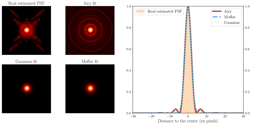
Figure 3: Example of the fitting of the true PSF on the empirical SPHERE/IRDIS data of the target HD 106906 reduced with RHAPSODIE. Observed PSF in H band (upper left) and different parametrization (Airy, Gaussian, and Moffat). Intensities are in log-scale to enhance the faint diffraction patterns.

4.3 Polarization calibration

When the light is reflected by the optical devices in the instrument, some instrumental polarization is introduced, resulting in a loss of polarized intensity and cross-talk contamination between Stokes parameters $Q$ and $U$.

The classical method to compensate for this instrumental polarization is to employs the azimuthal $Q_{\phi}$ and $U_{\phi}$ parameters to reduce the noise floor in the image (Avenhaus et al. 2014). Because this method is limited to face-on disks, we instead use the method developed by van Holstein et al. (2020) which rely on the pre-computed calibration of the instrumentation polarization as a function of the observational configurations. The pipeline IRDAP (van Holstein et al. 2020) yields the possibility to determine and correct the instrumental polarization in the signal reconstruction, yet this reconstruction requires to estimate first the $Q$ and $U$ parameters, to perform the instrumental polarization correction. After computing the double difference, IRDAP uses a Mueller matrix model of the instrument carefully calibrated using real on sky data to correct for the polarized intensity $I^{\text{p}}$ (created upstream of the HWP) and crosstalk of the telescope and instrument to compute the model-corrected $Q$ and $U$ images.

Using IRDAP, we estimate the instrumental transmission parameters $(\nu_{j,k,l})_{j\in\{1,\;2\},k\in\llbracket 1,K\rrbracket,\ell\in\llbracket 1,L\rrbracket}$ from the Mueller matrix to calibrate the instrumental polarization in our datasets.

IRDAP also determines the corresponding uncertainty by measuring the stellar polarization for each HWP cycle individually and by computing the standard error of the mean over the measurements. Finally, IRDAP creates an additional set of $Q$ and $U$ images by subtracting the measured stellar polarization from the model-corrected $Q$ and $U$ images. We use a similar method to correct for the stellar polarization which is responsible for strong light pollution at small separation in particular for faint disks such as debris disks. The contribution of this stellar light is estimated as different factors of $I^{\text{u}}$ in both $Q$ and $U$, respectively $\varepsilon_{Q}$ and $\varepsilon_{U}$. We estimate this stellar contribution by using a pixel annulus $\Omega$ located at a separation where there is no disk signal (either near the edge of the coronograph or at the separation corresponding to the adaptive optics cut-off frequency). Both corrections factors $\varepsilon_{Q}$ and $\varepsilon_{U}$ as follow:

$$\begin{cases}\varepsilon_{Q}=\big{(}\sum_{n\in\Omega}Q_{n}/I^{\text{u}}_{n}\big{)}/N_{\Omega}\\ \varepsilon_{U}=\big{(}\sum_{n\in\Omega}U_{n}/I^{\text{u}}_{n}\big{)}/N_{\Omega},\end{cases}$$ (25)

where $N_{\Omega}$ is the number of pixels of the ring $\Omega$. We then compute $Q^{\text{cor}}=Q-\varepsilon_{Q}I^{\text{u}}$ and $U^{\text{cor}}=U-\varepsilon_{U}I^{\text{u}}$ in order to create an additional set of $Q^{\text{cor}}$ and $U^{\text{cor}}$ images by subtracting the measured stellar polarization from the model-corrected Q and U images.

5 Applications on high contrast polarimetric data

In this section, we will compare two RHAPSODIE configurations. The first configuration defined as without deconvolution, means that $I^{\text{det}}_{j,k,m}$ in the data fidelity term (14) does not include the convolution, leading to the simplification of the equations (9) and (10):

$$I^{\text{det}}_{j,k,m} =\sum_{\ell=1}^{3}\,\nu_{j,k,\ell}\,\sum_{n=1}^{N}\,(\mathbf{T}_{j,k})_{m,n}\,S_{\ell,n}\,,$$ (26)

(i.e., $\mathbf{A}_{k}$ is the identity). Such a configuration of RHAPSODIE aims to be comparable to the state-of-the-art methods (i.e., Double Difference and IRDAP). These methods do not include any deconvolution and we aim to show that RHAPSODIE also performs well in such a case.

The second configuration defined as with deconvolution states for the full RHAPSODIE capabilities. Such a configuration of RHAPSODIE aims to show the benefits of the global model compared to an a posteriori deconvolution to improve the angular resolution.

5.1 Application on synthetic data

The performance of the linear and non-linear methods are first evaluated on synthetic datasets, without (resp. with) the deconvolution displayed on Fig. 4, Fig. 5 and Fig. 6 (resp. Fig. 7, Fig. 8 and Fig. 9). These datasets are composed of unpolarized residual stellar flux, mixed with unpolarized and polarized disk flux. We produce several synthetic datasets following steps given in Appendix A, for different ratios of the polarization of the disk, called $\tau^{\text{disk}}$ and defined in the equation (30).

The results of the RHAPSODIE methods are compared to the results obtained with the classical Double Difference method (Tinbergen 2005; Avenhaus et al. 2014). The Double Difference is applied on recentered and rotated datasets with the bad pixels interpolated. For the comparison with deconvolution, the results of the Double Difference are deconvolved after the reduction. In order to provide fair comparisons with RHAPSODIE, we propose to use an inverse approach rather than applying a high-pass spatial filtering. The deconvolved Double Difference reconstructions are obtained by solving the following problem:

$$(\widehat{Q},\widehat{U})\in \operatorname*{arg\,min}_{(Q,U)\in\mathbb{R}^{N}\times\mathbb{R}^{N}}\Bigg{[}\|\widehat{Q}^{\text{D. D.}}-\mathbf{A}Q\|^{2}+\|\widehat{U}^{\text{D. D.}}-\mathbf{A}U\|^{2}$$

$$\quad+\lambda_{(Q+U)^{\text{D. D.}}}f_{(Q+U)^{\text{D. D.}}}(Q,U)\Bigg{]}$$ (27)

where $\widehat{Q}^{\text{D. D.}}$ and $\widehat{U}^{\text{D. D.}}$ are the Stokes parameters reconstructed with the Double Difference and $\mathbf{A}$ represents the convolution by the PSF. This deconvolution method performs the deconvolution of Stokes parameters $Q$ and $U$ jointly in order to sharpen the polarized intensity image, but does not recover the polarization signal lost by averaging over close-by polarization signals with opposite sign and may even introduce artificial structures that are not present in the original source.

For the reconstruction with RHAPSODIE, the hyperparameters of regularization $\lambda_{\rho}$, and $\mu_{\rho}$ are chosen in order to minimize the total Mean Square Error (MSE), i.e. the sum of the MSE between each estimated parameter $\widehat{I^{\text{u}}}$, $\widehat{I^{\text{p}}}$ and $\widehat{\theta}$, obtained from $\widehat{\boldsymbol{X}}$ from Eq. (6), and the ground truth $I^{\text{u}}_{\text{gt}}$, $I^{\text{p}}_{\text{gt}}$ and $\theta_{\text{gt}}$. The total MSE is given by:

$$\textrm{MSE}^{\text{tot}} =\sum_{n=1}^{N_{I^{\text{u}}}}\mathbb{E}\Big{[}\big{(}\widehat{I^{\text{u}}}-I^{\text{u}}_{\text{gt}}\big{)}^{2}\Big{]}$$

$$\quad+\sum_{n=1}^{N_{I^{\text{p}}}}\mathbb{E}\Big{[}\big{(}\widehat{I^{\text{p}}}-I^{\text{p}}_{\text{gt}}\big{)}^{2}\Big{]}$$

$$\quad+\sum_{n=1}^{N_{\theta}}\mathbb{E}\Big{[}\textrm{angle}\big{(}\mathrm{e}^{2\mathrm{i}(\widehat{\theta}-\theta_{\text{gt}})}\big{)}^{2}\Big{]}.$$ (28)

where, $N_{I^{\text{u}}}$, $N_{I^{\text{p}}}$, and $N_{\theta}$ are the number of pixels with signal of interest in the respective $I^{\text{u}}$, $I^{\text{p}}$, and $\theta$ maps.

For the deconvolution of the Double Difference results, $\lambda_{(Q+U)^{\text{D. D.}}}$ and $\mu_{(Q+U)^{\text{D. D.}}}$ are chosen to minimize only the sum of the MSE on $I^{\text{u}}$ and $\theta$.

For the reconstructions without the deconvolution, Fig. 4 and Fig. 5 show that the reconstructions are less noisy with RHAPSODIE. The inner circle is always better reconstructed. Moreover, the non-linear reconstruction (i.e., minimization on $I^{\text{u}}$, $Q$ and $U$) is better than the linear when $\tau^{\text{disk}}$ grows. In both configurations of RHAPSODIE (non-linear and linear), the thin ring is not as well reconstructed as with the Double Difference. It is possible to recover such sharper structure with RHAPSODIE, by reducing the regularization weight (i.e., reducing the hyperparameter $\lambda_{Q+U}$). However, if $\lambda_{Q+U}$ is too small, the data will be overfitted and the noise in the reconstructed images will be amplified. It is thus necessary to keep a good trade-off between a smooth solution and a solution close to the data. Classically, minimizing the MSE is a good trade-off between underfitting and overfitting. The MSE curves in Fig. 6 are coherent with the observations. When $\tau^{\text{disk}}=25\%$, the non-linear RHAPSODIE MSE and Double Difference MSE are equivalent, but on the reconstructions, we can see that if the thin circle is better reconstructed with the Double Difference, the inner circle is better reconstructed with RHAPSODIE. Moreover, we can see that the angle error is more than three-time smaller with RHAPSODIE compared to the Double Difference error.

For the reconstructions with the deconvolution, the RHAPSODIE methods better reconstructions of the polarized intensity as shown on the reconstructions in Fig. 7, mostly for the inner ring, even if the background is less biased with the proposed deconvolved Double Difference (as shown on the error maps in Fig. 8). In fact, as shown on the MSE displayed in Fig. 9, for $\tau^{\text{disk}}=3\%$, RHAPSODIE delivers a more accurate polarized intensity estimation. The errors of the reconstructions are larger for the Double Difference than for the RHAPSODIE methods. The RHAPSODIE methods also allow us to achieve a better reconstruction of the angle of polarization, mostly with the non-linear estimation. The non-linear reconstruction appears to be more efficient as being not polluted by the artifacts of deconvolution of the unpolarized point source companion as seen on Fig. 8. Even if according to the MSE in Fig. 9, for $\tau^{\text{disk}}=25\%$, the MSE is smaller for the linear RAPSODIE. in fact, the space between the outer ring and the thin ring is better reconstructed with such a configuration (see Fig. 7 and Fig. 8).

Figure 4: Visual comparison of the reconstructed polarized intensity $I^{\text{p}}$ with the state-of-the-art Double Difference and the RHAPSODIE methods without deconvolution.

Figure 5: Maps of errors of the reconstructions displayed on Fig. 4. These errors are obtained as the difference between the true and the reconstructed images.

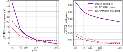
Figure 6: Comparison of the MSE between the true map and the estimated map of the polarized intensity $I^{\text{p}}$ and of the angle of polarization $\theta$ for the Double Difference and the linear and non-linear RHAPSODIE methods without deconvolution.

Figure 7: Visual comparison of the reconstructed polarized intensity $I^{\text{p}}$ with the state-of-the-art Double Difference and the RHAPSODIE methods with deconvolution.

Figure 8: Maps of errors of the reconstructions displayed on Fig. 7. These errors are obtained as the difference between the true and the reconstructed images.

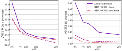
Figure 9: Comparison of the MSE between the true map and the estimated map of the polarized intensity $I^{\text{p}}$ and of the angle of polarization $\theta$ for the Double Difference and the linear and non-linear RHAPSODIE methods with deconvolution.

According to these results, the RHAPSODIE methods are better than the state-of-the-art methods, in particular the non-linear RHAPSODIE method. The benefits of our contribution is clearly visible in the case of faint disks and structures which are the most common on astrophysical data. This is why in the following section dedicated to the astrophysical data, we select the non-linear RHAPSODIE method with manual selection of the hyperparameters.

5.2 Astrophysical data

RHAPSODIE was applied to several IRDIS datasets dedicated to protoplanetary, transition and debris disks, to test the efficiency of our method and to compare it to the state-of-the-art method. For each reconstruction, we present the map of the projected intensities, by using the standard azimuthal Stokes parameters $Q_{\phi}$ and $U_{\phi}$ estimated from:

$$\begin{cases}Q_{\phi}=Q_{n}\cos\left(2\psi_{n}\right)+U_{n}\sin\left(2\psi_{n}\right)\\ U_{\phi}=U_{n}\cos\left(2\psi_{n}\right)-Q_{n}\sin\left(2\psi_{n}\right),\end{cases}$$ (29)

with $\psi_{n}=\arctan\left(\frac{n_{1}-n^{\text{center}}_{1}}{n_{2}-n^{\text{center}}_{2}}\right)$ where $\left(n_{1},n_{2}\right)$ denotes the row and the column indices of the $n$-th pixel in the map and $\left(n_{1}^{\text{center}},n_{2}^{\text{center}}\right)$ those of the pixel center. We also present the maps of polarized intensities $I^{\text{p}}$ and the angles of polarization $\theta$ estimated by the different methods.

Target	Date	Filter	$\Delta_{t}$ (s)	HWP cycles	$K^{\text{miss}}$	$\Delta_{t}^{\text{tot}}$ (s)	seeing	$\tau_{0}$ (ms)
TW Hydrae	$2015$-$04$-$01$	H	$16$	$22$	$13$	$5424$	1.15	2.2
IM Lupus	$2016$-$03$-$14$	H	$64$	$6$	$7$	$2624$	1.40	2.7
MY Lupus	$2016$-$03$-$16$	H	$64$	$7$	$18$	$2432$	1.63	1.5
RY Lupus	$2016$-$05$-$27$	H	$32$	$8$	$0$	$4096$	0.65	3.3
T Chae	$2016$-$02$-$20$	H	$32$	$30$	$0$	$3840$	1.8	2.2
RXJ 1615	$2016$-$03$-$15$	H	$64$	$11$	$7$	$5184$	0.7	4.1
HD 106906	$2019$-$01$-$17/18/20$	H	$32$	$42$	$0$	$5376$	0.54	14.0
HD 61005	$2015$-$05$-$02$	H	$16$	$12$	$16$	$2816$	1.5	3.2
AU MIC	$2017$-$06$-$20$	J	$16$	$23$	$0$	$11776$	1.4	2.2

Table 4: Information of the datasets used for the target reconstruction: the name of the target, the date of the observation, the filter used, the exposition time $\Delta_{t}$ for one acquisition, the number of cycles of HWP, the number of frame missing or removed $K^{\text{miss}}$, the total exposition time of the observation $\Delta_{t}^{\text{tot}}$ considering $K^{\text{miss}}$, the seeing, and observation conditions $\tau_{0}$. The total number of frames in each dataset is given by $K=\Delta_{t}^{\text{tot}}\,/\,\Delta_{t}+K^{\text{miss}}$.

Target	$\lambda_{I^{\text{u}}}^{\text{no-dec}}$	$\lambda_{Q+U}^{\text{no-dec}}$	$\mu_{I^{\text{u}}}^{\text{no-dec}}$	$\mu_{Q+U}^{\text{no-dec}}$	$\lambda_{I^{\text{u}}}^{\text{dec}}$	$\lambda_{Q+U}^{\text{dec}}$	$\mu_{I^{\text{u}}}^{\text{dec}}$	$\mu_{Q+U}^{\text{dec}}$	PSF
TW Hydrae	$10^{4.0}$	$10^{4.0}$	$10^{-4.0}$	$10^{-4.0}$	$10^{4.0}$	$10^{4.0}$	$10^{-5.0}$	$10^{-5.0}$	Moffat
IM Lupus	$10^{3.0}$	$10^{4.0}$	$10^{-0.8}$	$10^{-4.0}$	$10^{5.0}$	$10^{5.5}$	$10^{-3.0}$	$10^{-3.0}$	Airy
MY Lupus	$10^{2.0}$	$10^{0.4}$	$10^{-0.7}$	$10^{-3.6}$	$10^{1.0}$	$10^{0.5}$	$10^{-3.0}$	$10^{-3.0}$	Moffat
RY Lupus	$10^{4.0}$	$10^{5.5}$	$10^{-3.0}$	$10^{-3.0}$	$10^{5.0}$	$10^{3.0}$	$10^{-3.0}$	$10^{-3.0}$	Moffat
T Chae	$10^{0.0}$	$10^{-1.0}$	$10^{-3.0}$	$10^{-3.0}$	$10^{0.5}$	$10^{-1.0}$	$10^{-2.0}$	$10^{-2.0}$	Moffat
RXJ 1615	$10^{0.0}$	$10^{0.0}$	$10^{-4.0}$	$10^{1.0}$	$10^{1.0}$	$10^{-1.5}$	$10^{-3.0}$	$10^{-3.0}$	Moffat
HD 106906	$10^{2.5}$	$10^{1.5}$	$10^{-4.0}$	$10^{-4.0}$	$10^{5.0}$	$10^{1.7}$	$10^{2.2}$	$10^{-1.8}$	Airy
HD 61005	$10^{5.0}$	$10^{4.1}$	$10^{-0.7}$	$10^{-3.4}$	$10^{5.0}$	$10^{4.1}$	$10^{-0.7}$	$10^{-3.9}$	Moffat
AU MIC	$10^{5.0}$	$10^{4.3}$	$10^{-4.2}$	$10^{-3.2}$	$10^{5.0}$	$10^{4.3}$	$10^{-1.2}$	$10^{-4.2}$	Moffat

Table 5: Informations of the parameters used for the target reconstruction presented in this section: the name of the target and the values of the hyperparameters $\lambda_{I^{\text{u}}}^{\text{no-dec}}$, $\lambda_{Q+U}^{\text{no-dec}}$, $\mu^{\text{no-dec}}$ (resp. $\lambda_{I^{\text{u}}}^{\text{dec}}$, $\lambda_{Q+U}^{\text{dec}}$, $\mu^{\text{dec}}$) used for the reconstruction with RHAPSODIE without deconvolution (resp. with deconvolution), and the parametrization model of the PSF used.

First, the reconstructions of the target TW Hydrae with the Double Difference and RHAPSODIE without deconvolution are compared in the Fig.10, without and with the correction of the instrumental polarization. The images are scaled by the square of the separation to account for the drop-off of stellar illumination with distance.

The instrumental polarization in this dataset introduces a polarization rotation and an attenuation (loss of polarization signal) of the intensity with varying time during the observations which can be monitored easily because the disk is face-on. If uncorrected, the combination of data from multiple polarimetric cycles will result in very poorly constrained polarimetric intensity measurements. When we correct the instrumental polarization (see Fig. 10(c)) by using the IRDAP method, these effects are compensated and the disk reconstructed is more accurate (Fig. 10(c) (iii). As a result, the contamination of the $U_{\phi}$ signal from cross-talk is decreased and becomes negligible as seen in Fig. 10(c) (iii).

The comparison with van Boekel et al. (2017); de Boer et al. (2020) shows that our method is less impacted by the bad pixels and improves the disk SNR in the area where the signal is low. On the other hand, it is slightly more sensitive to detector flat calibration accuracy. It is worth noticing that IRDAP has a dedicated correction of the detector response nonuniformity (flat field variation between the detector column) for the various amplifiers that is not implemented in RHAPSODIE. However, the flat calibration of observations more recent than 2016 have improved and do allow better calibration and as a consequence do not impact our method efficiency anymore.

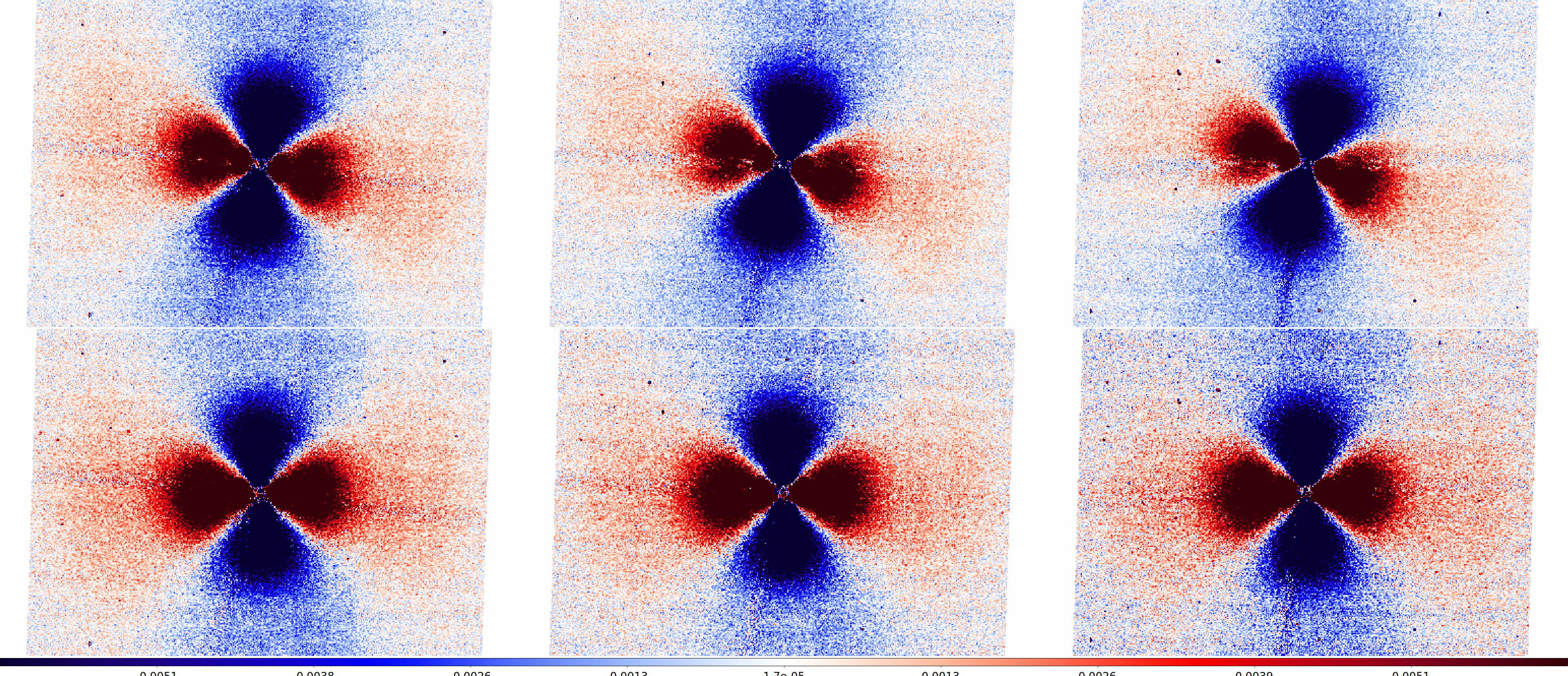
(a) Stokes parameter $Q$.

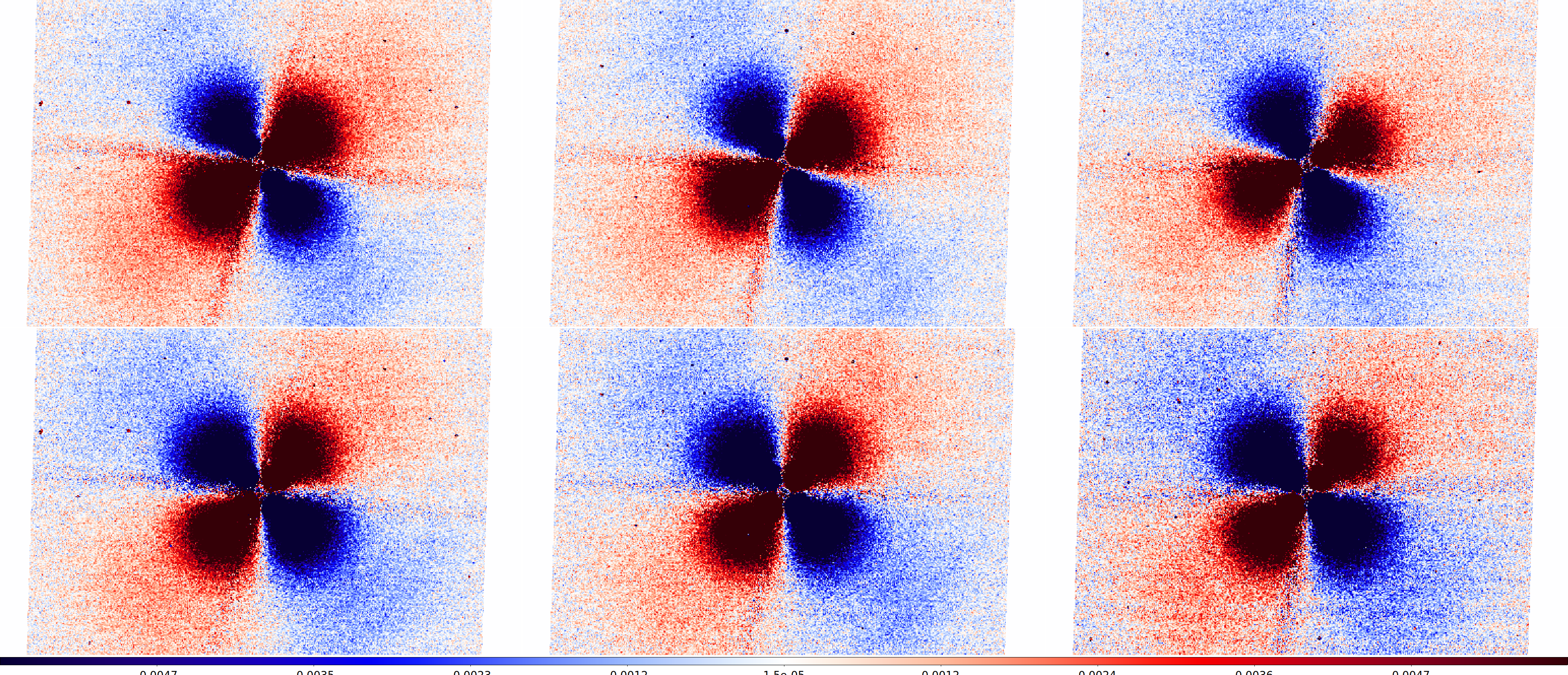
(b) Stokes parameter $U$.

(c) Azimutal Stokes parameters displayed in arcseconds : (i) Double Difference, (ii) Double Difference with the instrumental polarization correction, (iii) RHAPSODIE which includes by default the instrumental polarization correction. The intensities are multiplied in each pixel by the distance to the star $r^{2}$.

Figure 10: Reconstruction of the $Q$ (a) and $U$ (b) parameters of the target TW Hydrae, for the first three cycle of HWP rotation, without (upper row) and with (lower row) the correction of the polarization. Without the correction, both $Q$ and $U$ are rotated and attenuated. The $Q_{\phi}$ and $U_{\phi}$ images reconstructed from the entire dataset are presented in (c). All the reconstructions are done without deconvolution to demonstrate mainly the efficiency of the instrumental polarization correction and the benefits of RHAPSODIE.

Figure 11: Reconstructions of the polarized intensity $I^{\text{p}}$ of the protoplanetary disks TW Hydrae, IM Lupus, and MY Lupus. From the left to the right, the reconstructions have been obtained with the Double Difference, RHAPSODIE without deconvolution and RHAPSODIE with deconvolution. The maps are displayed in logarithmic scale and normalized in contrast to the unpolarized stellar flux. The pixels lying underneath the coronograph are masked in black. North is up and East is to the left in all frames.

Figure 12: Reconstructions of the polarization angle $\theta$ of the protoplanetary disks TW Hydrae, IM Lupus, and MY Lupus. From the left to the right, the reconstructions have been obtained with the Double Difference, RHAPSODIE without deconvolution and RHAPSODIE with deconvolution. The maps are displayed in logarithmic scale and normalized in contrast to the unpolarized stellar flux. The pixels lying underneath the coronograph are masked in black. North is up and East is to the left in all frames.

Figure 13: Reconstructions of the polarized intensity $I^{\text{p}}$ of the transition disks RY Lupus, T Chae, and RXJ 1615. From the left to the right, the reconstructions have been obtained with the Double Difference, RHAPSODIE without deconvolution and RHAPSODIE with deconvolution. The maps are displayed in logarithmic scale and normalized in contrast to the unpolarized stellar flux. The pixels lying underneath the coronograph are masked in black. North is up and East is to the left in all frames.

Figure 14: Reconstructions of the polarization angle $\theta$ of the transition disks RY Lupus, T Chae, and RXJ 1615. From the left to the right, the reconstructions have been obtained with the Double Difference, RHAPSODIE without deconvolution and RHAPSODIE with deconvolution. The maps are displayed in logarithmic scale and normalized in contrast to the unpolarized stellar flux. The pixels lying underneath the coronograph are masked in black. North is up and East is to the left in all frames.

Figure 15: Reconstructions of the polarized intensity $I^{\text{p}}$ of the debris disks HD 106906, HD 61005, and AU MIC. From the left to the right, the reconstructions have been obtained with the Double Difference, RHAPSODIE without deconvolution and RHAPSODIE with deconvolution. The maps are displayed in logarithmic scale and normalized in contrast to the unpolarized stellar flux. The pixels lying underneath the coronograph are masked in black. North is up and East is to the left in all frames.

Figure 16: Reconstructions of the polarized intensity $I^{\text{p}}$ of the debris disks HD 106906, HD 61005, and AU MIC. From the left to the right, the reconstructions have been obtained with the Double Difference, RHAPSODIE without deconvolution and RHAPSODIE with deconvolution. The maps are displayed in logarithmic scale and normalized in contrast to the unpolarized stellar flux. The pixels lying underneath the coronograph are masked in black. North is up and East is to the left in all frames.

Figure 17: $Q_{\phi}$ and $U_{\phi}$ projections of the reconstructions of RY Lupus and T Chae. The maps are displayed in symmetrical logarithmic scale and normalized in contrast to the unpolarized stellar flux. The coronograph is masked in white.

The efficiency of the method we have developed is demonstrated on the Figures 11, 12, 13, 14, 15, 16, and Fig. 17. Fig. 11 and Fig. 12 present the Double Difference and RHAPSODIE reconstructions of the protoplanery disks TW Hydrae (van Boekel et al. 2017), IM Lupus (Avenhaus et al. 2018) and MY Lupus (Avenhaus et al. 2018). Fig. 13, 14, and Fig. 17 present RHAPSODIE reconstructions of transition disks RY Lupus (Langlois et al. 2018) and T Chamaeleontis (Pohl et al. 2017). Fig. 13, 14 also present RHAPSODIE reconstructions of transition disk RXJ 1615 (de Boer et al. 2016). Fig. 15 and Fig. 16 present the RHAPSODIE reconstructions of the debris disks HD 106906 (Kalas et al. 2015; Lagrange et al. 2016), HD 61005 (Olofsson et al. 2016), and AU Mic (Boccaletti et al. 2018).These reconstructions are all normalized in contrast to the unpolarized stellar flux (estimated when registering the PSF off-centered from the coronograph) by taking into account the transmission of the neutral-density filter used when registering the PSF to prevent saturation.

The contrast between the selected disks polarized light and their host stars unpolarized light responsible for the level of stellar pollution are also very different (ranging from $3\cdot 10^{-2}$ to $8\cdot 10^{-6}$). The achievable contrast is more favorable for highly inclined disk such as MY Lup on Fig. 11 because in such a case, the star likely shines partially through the disk, which is dimming the starlight and thus decreasing the contrast between the star and the disk.

In all cases, our method produces high-quality reconstructions of the disk polarized signal and minimizes the artifacts from bad pixels. The comparison of these reductions with the state-of-the-art confirms the benefits of our method but it is more difficult to quantify the gain on real data not knowing the truth and should be strengthened by using numerical models of these objects. In addition, our method can produce deblurred results which clearly enhances the angular resolution and is beneficial for interpreting the disk morphology and for studying its physical properties. In all cases, the deconvolution sharpens the polarized intensity image, helps to recover the polarization signal lost by averaging over close-by polarization signals with opposite sign, and does not introduce artificial structures that are not present in the original source (see Fig. 13 (RY Lup)). As mentioned before the hyperparameters could be further tuned to adjust the smoothing of the deconvolved images according to the required noise/angular resolution trade-off.

For several of these disks (IM Lup, MY Lup on Fig.11), the outer edge of the disk and thus the lower disk surface have been detected in Avenhaus et al. (2018) and are confirmed by our method. The deconvolution of these datasets allows to further highlight these fainter features, to enhance or reveal the midplane gaps in the case of T Cha (on Fig. 13) which was not identified by Pohl et al. (2017). The reason is that without deconvolution, the PSF smears light from the disk upper and lower sides into the midplane gap.

Except for Au Mic, the debris disk presented on Fig. 15 are much fainter in contrast than the protoplanetary or the transition disks in polarized intensity. As a consequence these datasets have required careful stellar polarization compensation. The HD 106906 debris disk is viewed close to edge-on in polarized light as reported in van Holstein et al. (2020); Esposito et al. (2020). The image clearly shows the known East-West brightness asymmetry of the disk, which was detected in total intensity (Kalas et al. 2015; Lagrange et al. 2016). Thanks to the deep dataset and good reconstruction, we also detect the backward-scattering far side of the disk to the west of the star, just south of the brighter near side of the disk. This feature is further highlighted by the deconvolution.

The reader may remark that the RHAPSODIE deblurred reconstructions of RXJ 1615 (on Fig. 13) and HD 106906 (on Fig. 15) seems noisier than without deconvolution. This is due to hyperparameters purposely chosen so as to achieve the best angular resolution with the side effect of slight noise amplification. Thus the noise is not negligible in the reconstruction. As shown in Fig. 2, increasing the regularization weight to smooth the background would lead to a loss of the thin structures.

We also analyzed two datasets (HD 61005 and Au Mic) taken under very bad conditions. For these two datasets, our method also proves to be efficient in using incomplete polarization cycles to recover the disk polarized signal, and to deconvolve this signal despite strong artifacts produced in addition by the rotating spiders (i.e., unmasked by the Lyot stop) when observing in field stabilized. The difference in the spider position during the polarimetric cycle results in an artificial polarimetric signal when using standard data reduction techniques. It is worth noticing that the strength of our method to deal with these artifacts comes from its ability to use weighted maps to account for them. For instance, the spiders are weighted by their variance during their rotation frame by frame in addition to the inclusion of a static bad pixel ponderation. As a result, the contribution of the spiders to the polarimetric signal when using our method is decreased compared to the other methods. The noise which is created by these spiders remains, as seen on Fig. 15, and can generate artifacts in the deconvolution as seen for HD 61005. Counteracting the artifacts caused by the spiders can be efficiently done by performing DPI observation in pupil tracking mode as proposed in van Holstein et al. (2017). We have also validated the efficiency of RHAPSODIE in such observations which allows a further gain in the reduction of the instrumental artifacts from the telescope spiders.

Another advantage of our method is its ability to use incomplete polarimetric cycles which are discarded by the classical methods. This capability of our method leads to an increase in SNR which was quantified more precisely using our model of the data in Denneulin (2020). To benefit from this improvement, the instrumental polarization has to remain small because incomplete polarimetric cycles do not benefit from the instrumental polarization compensation performed by estimating both couples $Q$ and $-Q$ (and $U$ and $-U$, respectively).

6 Conclusion

We developed a new method to extract the polarimetric signal using an inverse problems approach that exploits a model of the measured signal formation process. The method includes a weighted data fidelity term which takes into account the blur and the polarization due to the instrument, and effectively disentangles polarized signal of interest from stellar contamination. In order to avoid noise amplification in the minimization of the data fidelity term, an edge preserving smoothing penalization is added allowing to favor smooth estimates almost everywhere. The associated minimization problem is solved by standard optimization techniques. Our method enables to accurately measure the polarized intensity and angle of linear polarization of circumstellar disks by taking into account the noise propagation and the observed objects convolution. It has the capability to use incomplete polarimetry cycles (when the instrumental polarization is small) which enhances the sensitivity of these observations. It also takes proper account for bad pixels by using weighted maps instead of interpolating them. These bad pixels can cause systematic errors of several tenths of percent in the polarization measurements as shown by (van Holstein et al. 2021) In addition, the effect of bad pixel interpolation could also have some impact when reaching $0.1$% polarimetric accuracy.

We have validated the method on both simulated and archive data from SPHERE/IRDIS and compared its performances with the state-of-the-art methods. We have implemented the method in an end-to-end data-analysis package called RHAPSODIE. The method we developed improves the overall performances in particular at low SNR/small polarized flux compared to standard methods.

By increasing the sensitivity and including deconvolution, this method will allow for more accurate studies of the orientation and morphology of the disks, especially in the innermost regions. It also will enable more accurate measurements of the angle of linear polarization at low SNR, which would allow for more in-depth studies of dust properties. Finally, the method will enable more accurate measurements of the polarized intensity which is critical to construct scattering phase functions.

RHAPSODIE is the first regularized inverse approach implemented for high contrast polarimetric imaging. It demonstrates the benefits of advanced signal processing methods in this domain.

7 Acknowledgements

We acknowledge Rob Van Holstein for his help with the instrumental polarization correction based on careful instrumental calibrations he performed which are implemented in the IRDAP tool he developed. We also thank the anonymous referee for her/his careful reading of the manuscript as well as her/his insightful comments and suggestions.This work has made use of the SPHERE Data Centre, jointly operated by OSUG/IPAG (Grenoble), PYTHEAS/LAM/CeSAM (Marseille), OCA/Lagrange (Nice), Observatoire de Paris/LESIA (Paris), and Observatoire de Lyon (OSUL/CRAL). This work is supported by the French National Programms PNP and the Action Spécifique Haute Résolution Angulaire (ASHRA) of CNRS/INSU co-funded by CNES. The authors are grateful to the LABEX Lyon Institute of Origins (ANR-10-LABX-0066) of the Université de Lyon for its financial support within the program “Investissements d’Avenir” (ANR-11-IDEX-0007) of the French government operated by the National Research Agency (ANR). This paper is based on observations made with ESO Telescopes at the La Paranal Observatory under programme ID: 598.C-0359, 095.C-0273, 0102.C-0916, 096.C-0523, 097.C-0523, 096.C-0248.

Appendix A Synthetic dataset simulation

In order to evaluate the performance of the RHAPSODIE method, synthetic data have been created. These synthetic data are designed to reproduce astrophysical cases. First, the truth $N=128\times 128$ maps $I^{\text{u}}_{\text{gt}}$, $I^{\text{p}}_{\text{gt}}$ et $\theta_{\text{gt}}$ are created. Such a value of $N$ pixels fits the main Region Of Interest (ROI) size.

Figure 18: Total ratios of polarization $\tau^{\text{total}}$ maps, with respect to the total intensities, and SNR maps for the different values of disk polarized fractions $\tau^{\text{disk}}$.

The hardest disk structures to reconstruct are faint, small and lightly polarized structures, and consequently have high contrast with the unpolarized stellar intensity and a low SNR. This is why the synthetic environment we generated a disk with three rings of equal brightness but with a different contrast with the unpolarized stellar intensity. This disk is partially polarized with a linearly polarization $I^{\text{p}}$ and a polarization angle $\theta\in]-\pi,\pi]$ and an unpolarized component ${I^{\text{u}}}^{\text{disk}}$. The disk polarization ratio between both component is given by:

$$\tau^{\text{disk}}=\frac{I^{\text{p}}}{{I^{\text{u}}}^{\text{disk}}+I^{\text{p}}}.$$ (30)

These synthetic images are then combined as maps of Stokes parameters $I$, $Q$ and $U$.

The ${I^{\text{u}}}^{\text{disk}}$ component is mixed with the unpolarized ${I^{\text{u}}}^{\text{star}}$ stellar components and a point source companion (star close to the host star of different brightness). The unpolaized intensity is represented as $I^{\text{u}}={I^{\text{u}}}^{\text{star}}+{I^{\text{u}}}^{\text{disk}}$. It is important to keep in mind that unmixing both disk and stellar unpolarized components is not possible from DPI data without the diversity introduced by ADI. The $\tau^{\text{disk}}$ value used to synthetise datasets is thus inaccessible in practice from observational polarimetric datasets. To assert the case difficulty, one can then use the total polarization, given for all pixel $n\in\{1,\ldots,N\}$ by:

$$\tau^{\text{total}}(\boldsymbol{x}_{n})=\frac{I^{\text{p}}_{n}}{I^{\text{u}}_{n}+I^{\text{p}}_{n}},$$ (31)

and the Signal-to-Noise Ratio (SNR), given for all pixel $n\in\{1,\ldots,N\}$ by:

$$\textrm{SNR}(\boldsymbol{x}_{n})=\frac{\sqrt{K_{\alpha}}I^{\text{p}}_{n}}{\sqrt{(I^{\text{u}}_{n}+I^{\text{p}}_{n})/2+\sigma_{\text{ro}}^{2}}},$$ (32)

where $\sigma_{\text{ro}}^{2}$ is the read-out noise variance. The difference between $\tau^{\text{total}}$ and $\tau^{\text{disk}}$ is that the last one does not take into account the unpolarized star residuals. The figure 18 present the SNR maps and the maps of total polarization ratio of the synthetic parameters generated for different $\tau^{\text{disk}}$. At the center, where the unpolarized star residual are the brightest, the SNR and the total polarization ratio are the weakest especially in the case of small ${I^{\text{u}}}^{\text{disk}}$. Yet the SNR grows with the separation from the star center (like the stellar contribution or when the polarized contribution of the disk increases. Fig. 19 present the true simulated maps for $\tau^{\text{disk}}=10\%$.

Finally, to generate synthetic calibrated data, the Stokes maps are combined following the expression of the data physical model (12), with $K\times M$ noise realizations from a fixed random seed. The values of $10\%$ of the pixels, choosen randomly, are replaced by zeros to mimic bad pixel behaviours. The weights related to each acquisition are simulated at the same time following (15). The datasets are composed of $8$ HWP cycles, with $2$ acquisitions per positions in each cycles, leading to $16$ images per position of Half-Wave Plate (HWP). Thus, the total number of images per datasets is $K=64$.

Several datasets are created with $\tau^{\text{disk}}\in\{3\%,7\%,10\%,15\%,25\%\}$, corresponding to difficult cases for $\tau^{\text{disk}}<10\%$ and less difficult brighter cases above this threshold.

Before producing $K\times 2N$ noise realization on each dataset, the random seed is reset to the same value. This allow the reproducibility of the results. In fact this realization is obtained by the multiplication of the standard deviation of the pixel to a gaussian, centered and reduced gaussian realization. Since the random seed is the same for each dataset, the realization is the same for the given pixel, only the standard deviation changes.

In order to compare the results of the Double Difference to the results of the RHAPSODIE methods the dataset are pre-processed. The bad pixels are interpolated; then the left and right part of the images are cut, recentered and rotated.

Figure 19: Schematic describing the process of the data simulation. Starting from synthetic maps $I^{\text{u}}_{\text{gt}}$, $I^{\text{p}}_{\text{gt}}$, and $\theta_{\text{gt}}$ based on a disc model, we generate artificial calibrated and pre-processed datasets $\boldsymbol{d}$ and associated weights $\mathbf{W}$, illustrated here for $\tau^{\text{disk}}=10\%$.

References

- Adam et al. (2016) Adam, R., Ade, P. A., Aghanim, N., et al. 2016, A&A, 594, A8
- Akiyama et al. (2019) Akiyama, K., Alberdi, A., Alef, W., et al. 2019, ApJ Letters, 875, L4
- Avenhaus et al. (2018) Avenhaus, H., Quanz, S. P., Garufi, A., et al. 2018, ApJ, 863, 44
- Avenhaus et al. (2014) Avenhaus, H., Quanz, S. P., Schmid, H. M., et al. 2014, ApJ, 781, 87, arXiv: 1311.7088
- Benisty et al. (2015) Benisty, M., Juhasz, A., Boccaletti, A., et al. 2015, A&A, 578, L6
- Berdeu et al. (2020) Berdeu, A., Soulez, F., Denis, L., Langlois, M., & Thiébaut, É. 2020, A&A, 635, A90
- Beuzit et al. (2019) Beuzit, J.-L., Vigan, A., Mouillet, D., et al. 2019, A&A, 631, A155
- Biraud (1969) Biraud, Y. 1969, A&A, 1, 124
- Birdi et al. (2018) Birdi, J., Repetti, A., & Wiaux, Y. 2018, MNRAS, arXiv: 1801.02417
- Birdi et al. (2019) Birdi, J., Repetti, A., & Wiaux, Y. 2019, arXiv:1904.00663 [astro-ph], arXiv: 1904.00663
- Boccaletti et al. (2018) Boccaletti, A., Sezestre, E., Lagrange, A. M., et al. 2018, A&A, 614, A52
- Borde & Traub (2006) Borde, P. J. & Traub, W. A. 2006, ApJ, 638, 488
- Carrillo et al. (2012) Carrillo, R. E., McEwen, J. D., & Wiaux, Y. 2012, MNRAS, 426, 1223
- Charbonnier et al. (1997) Charbonnier, P., Blanc-Féraud, L., Aubert, G., & Barlaud, M. 1997, IEEE TIP, 6, 298
- Chierchia et al. (2014) Chierchia, G., Pustelnik, N., Pesquet-Popescu, B., & Pesquet, J.-C. 2014, IEEE Trans. on Image Process., 23, 5531
- Claudi et al. (2008) Claudi, R. U., Turatto, M., Gratton, R. G., et al. 2008, in Ground-based and Airborne Instrumentation for Astronomy II, Vol. 7014, International Society for Optics and Photonics, 70143E
- Combettes & Pesquet (2011) Combettes, P. & Pesquet, J.-C. 2011, 185
- Combettes & Wajs (2005) Combettes, P. L. & Wajs, V. R. 2005, Multiscale Model. Simul., 4, 1168
- de Boer et al. (2020) de Boer, J., Langlois, M., van Holstein, R. G., et al. 2020, A&A, 633, A63
- de Boer et al. (2016) de Boer, J., Salter, G., Benisty, M., et al. 2016, A&A, 595, A114
- de Boer et al. (2016) de Boer, J., Salter, G., Benisty, M., et al. 2016, A&A, 595, A114
- Deledalle et al. (2014) Deledalle, C.-A., Vaiter, S., Fadili, J., & Peyré, G. 2014, SIIMS, 7, 2448
- Denneulin (2020) Denneulin, L. 2020, PhD thesis, Lyon
- Denneulin et al. (2019) Denneulin, L., Langlois, M., Pustelnik, N., & Thiébaut, É. 2019, in GRETSI LILLE 2019
- Denneulin et al. (2020) Denneulin, L., Pustelnik, N., Langlois, M., Loris, I., & Thiébaut, É. 2020, iTwist, Nantes, France, Dec. 2-4, 2020.
- Dipierro et al. (2015) Dipierro, G., Price, D., Laibe, G., et al. 2015, MNRAS Letters, 453, L73
- Dohlen et al. (2008) Dohlen, K., Langlois, M., Saisse, M., et al. 2008, in Ground-based and Airborne Instrumentation for Astronomy II, Vol. 7014, International Society for Optics and Photonics, 70143L
- Eldar (2008) Eldar, Y. C. 2008, IEEE Trans. on Signal Process., 57, 471
- Esposito et al. (2020) Esposito, T. M., Kalas, P., Fitzgerald, M. P., et al. 2020, AJ, 160, 24
- Flasseur et al. (2019) Flasseur, O., Denis, L., Thiébaut, É., Olivier, T., & Fournier, C. 2019, in 2019 27th European Signal Processing Conference (EUSIPCO), IEEE, 1–5
- Garufi et al. (2017) Garufi, A., Benisty, M., Stolker, T., et al. 2017, arXiv preprint arXiv:1710.02795
- Ginski et al. (2016) Ginski, C., Stolker, T., Pinilla, P., et al. 2016, A&A, 595, A112
- Golub et al. (1979) Golub, G. H., Heath, M., & Wahba, G. 1979, Technometrics, 21, 215
- Haffert et al. (2019) Haffert, S. Y., Bohn, A. J., de Boer, J., et al. 2019, Nat Astron, 3, 749
- Hansen & O’Leary (1993) Hansen, P. C. & O’Leary, D. P. 1993, SISC, 14, 1487
- Högbom (1974) Högbom, J. 1974, A&A Supplement Series, 15, 417
- Kalas et al. (2015) Kalas, P. G., Rajan, A., Wang, J. J., et al. 2015, ApJ, 814, 32
- Keppler et al. (2018) Keppler, M., Benisty, M., Müller, A., et al. 2018, A&A, 617, A44
- Keppler et al. (2019) Keppler, M., Teague, R., Bae, J., et al. 2019, A&A, 625, A118
- Lagrange et al. (2016) Lagrange, A. M., Langlois, M., Gratton, R., et al. 2016, A&A, 586, L8
- Langlois et al. (2014) Langlois, M., Dohlen, K., Vigan, A., et al. 2014, in Ground-based and Airborne Instrumentation for Astronomy V, Vol. 9147, International Society for Optics and Photonics, 91471R
- Langlois et al. (2018) Langlois, M., Pohl, A., Lagrange, A.-M., et al. 2018, A& A, 614, A88
- Lefkimmiatis et al. (2013) Lefkimmiatis, S., Ward, J. P., & Unser, M. 2013, IEEE Trans. on Image Process., 22, 1873
- Macintosh et al. (2014) Macintosh, B., Graham, J. R., Ingraham, P., et al. 2014, proceedings of the National Academy of Sciences, 111, 12661
- Mahalanobis (1936) Mahalanobis, P. C. 1936, National Institute of Science of India
- Maire et al. (2016) Maire, A.-L., Langlois, M., Dohlen, K., et al. 2016, in Ground-based and Airborne Instrumentation for Astronomy VI, Vol. 9908, International Society for Optics and Photonics, 990834
- Marois et al. (2006) Marois, C., Lafreniere, D., Doyon, R., Macintosh, B., & Nadeau, D. 2006, ApJ, 641, 556
- Milli et al. (2019) Milli, J., Engler, N., Schmid, H. M., et al. 2019, 13
- Molina (1994) Molina, R. 1994, IEEE Transactions on Pattern Analysis and Machine Intelligence, 16, 1122
- Muto et al. (2012) Muto, T., Grady, C., Hashimoto, J., et al. 2012, ApJ Letters, 748, L22
- Nocedal & Wright (1999) Nocedal, J. & Wright, S. J. 1999, Numerical optimization, Springer series in operations research (New York: Springer)
- Olofsson et al. (2016) Olofsson, J., Samland, M., Avenhaus, H., et al. 2016, A&A, 591, A108
- Pairet et al. (2019) Pairet, B., Jacques, L., & Cantalloube, F. 2019, Proceedings of SPARS’19, 1, 1
- Perrin et al. (2015) Perrin, M. D., Duchene, G., Millar-Blanchaer, M., et al. 2015, ApJ, 799, 182
- Pinte et al. (2019) Pinte, C., van der Plas, G., Menard, F., et al. 2019, Nat Astron, 3, 1109, arXiv: 1907.02538
- Pohl et al. (2017) Pohl, A., Sissa, E., Langlois, M., et al. 2017, A&A, 605, 17
- Price et al. (2018) Price, D. J., Cuello, N., Pinte, C., et al. 2018, MNRAS, 477, 1270, arXiv: 1803.02484
- Pustelnik et al. (2016) Pustelnik, N., Benazza-Benhayia, A., Zheng, Y., & Pesquet, J.-C. 2016, in Wiley Encyclopedia of Electrical and Electronics Engineering (Hoboken, NJ, USA: John Wiley & Sons, Inc.), 1–34
- Quanz et al. (2013) Quanz, S. P., Avenhaus, H., Buenzli, E., et al. 2013, ApJ Letters, 766, L2
- Ramani et al. (2008) Ramani, S., Blu, T., & Unser, M. 2008, IEEE TIP, 17, 1540
- Rudin et al. (1992) Rudin, L. I., Osher, S., & Fatemi, E. 1992, Physica D: Nonlinear Phenomena, 60, 259
- Schmid et al. (2018) Schmid, H. M., Bazzon, A., Roelfsema, R., et al. 2018, A&A, 619, A9
- Sissa et al. (2018) Sissa, E., Olofsson, J., Vigan, A., et al. 2018, A&A, 613, L6
- Smirnov (2011) Smirnov, O. M. 2011, A&A, 527, A106
- Starck et al. (2003) Starck, J.-L., Donoho, D. L., & Candès, E. J. 2003, A&A, 398, 785
- Stein (1981) Stein, C. M. 1981, The annals of Statistics, 1135
- Tarantola (2005) Tarantola, A. 2005, Inverse problem theory and methods for model parameter estimation (SIAM)
- Thiébaut (2002) Thiébaut, E. 2002, in Astronomical Data Analysis II, Vol. 4847, International Society for Optics and Photonics, 174–183
- Thiébaut & Conan (1995) Thiébaut, E. & Conan, J.-M. 1995, JOSA A, 12, 485
- Tikhonov (1963) Tikhonov, A. N. 1963, Soviet Mathematics Doklady
- Tinbergen (2005) Tinbergen, J. 2005, Astronomical Polarimetry (Cambridge University Press), google-Books-ID: SAS4JzAaMxkC
- Titterington (1985) Titterington, D. M. 1985, A&A, 144, 381
- van Boekel et al. (2017) van Boekel, R., Henning, T., Menu, J., et al. 2017, ApJ, 837, 132
- van Holstein et al. (2020) van Holstein, R. G., Girard, J. H., de Boer, J., et al. 2020, A&A, 633, A64
- van Holstein et al. (2017) van Holstein, R. G., Snik, F., Girard, J. H., et al. 2017, Techniques and Instrumentation for Detection of Exoplanets VIII, 38, arXiv: 1709.07519
- van Holstein et al. (2021) van Holstein, R. G., Stolker, T., Jensen-Clem, R., et al. 2021, A&A, 647, A21
- Vigan et al. (2014) Vigan, A., Langlois, M., Dohlen, K., et al. 2014, in Ground-based and Airborne Instrumentation for Astronomy V, Vol. 9147, International Society for Optics and Photonics, 91474T