Continuous Control of Conservatism for Robust Optimization by Adjustable Regret

Abstract

It is commonly recognized that a major issue of robust optimization is the tendency to produce overly conservative solutions. To address this issue, a new regret-based criterion with a single control parameter is proposed and axiomatized to offer smooth control of conservatism in a wide range without tampering with the uncertainty set. This criterion has many appealing analytical properties, such as decreasing conservatism with regard to the control parameter, which makes it a unique choice for fine control of conservatism. Tractability for robust linear programs with this criterion is established by reformulating them into those with the maximin criterion, for which tractable solution schemes and theoretical results are actively developed in the literature. Closed-form solutions are obtained for the robust one-way trading problem with this criterion, leading to a greatly simplified competitive ratio analysis. Numerical experiments are conducted to demonstrate smooth control of conservatism and the effects on revenue and risk.

[inst1]organization=Peking University HSBC Business School,addressline=Xili University Town, city=Shenzhen, postcode=00000, state=Guangdong, country=China

1 Introduction.

Robust optimization (RO) in the broad sense deals with decision-making under data uncertainty without requiring an exact distribution, which is, in contrast, a prerequisite for stochastic programming. The survey of Gabrel et al., (2014) covers topics from distributional RO to the traditional or narrow-sensed RO that features an uncertainty set and a maximin reward or minimax cost criterion. RO is often considered more practical and powerful in applications where an exact distribution is difficult to estimate, due to little or inaccurate data, or nonstationarity of the underlying stochastic process. The traditional RO is initially developed in Soyster, (1973), which proposes a robust counterpart for a linear programming (LP) model to address the feasibility concern, as data uncertainty can cause constraint violation. A large branch of studies follows Soyster, (1973) to derive tractable reformulations that provide insights into robust solutions as well as probabilistic guarantees of feasibility (see Ben-Tal and Nemirovski, 2008 and Bertsimas et al., 2011 for comprehensive surveys and Ben-Tal et al., 2009 for a book treatment).

As much performance is often sacrificed for robustness, it raises grave concern about optimality and over-conservatism, which is, for example, considered as a major reason preventing airlines from adopting robust revenue management methods in Vinod, (2021). The robust counterpart of Soyster, (1973) is quickly found to be overly conservative with a severe performance deterioration, which is caused by providing complete protection from all adverse scenarios. Such protection may be justifiable in engineering where infeasibility can cause a doomed satellite launch or a destroyed unmanned robot. However, adverse events in business like low demand or supply do not bring about such disastrous consequences, thus protection can be made by a smaller and more flexible uncertainty set, with a lower probabilistic guarantee of feasibility in exchange for better performance. Significant progress in the theory of RO was then made in this regard for models with ellipsoidal uncertainty sets by Ben-Tal and Nemirovski, (1998, 1999, 2000), El-Ghaoui and Lebret, (1997), and El Ghaoui et al., (1998). As such models are nonlinear and much more demanding computationally than linear models, Bertsimas and Sim, (2004) proposes the uncertainty budget method that can fully control the uncertainty set for every constraint while maintaining linearity. A drawback of these approaches is that they tamper with the uncertainty set to trade-off between robustness and conservatism, which can be difficult to balance, and may even be impossible in some engineering cases.

This paper tackles the issue of over-conservatism from a new angle without touching the uncertainty set by proposing a new decision criterion. Three criteria are commonly used in research and practices due to their good analytical properties and computational tractability, but none of them offers fine control of conservatism. The earliest maximin reward criterion is employed in traditional RO and often considered as the Achilles’ heel, as it focuses entirely on worst-case profits and completely ignores all plausible opportunities for higher profits, which can lead to very conservative solutions. To alleviate this issue, the absolute and relative regret criteria are proposed on the basis of regret experienced by decision-makers once they realized what could have been the best action in hindsight (Kouvelis and Yu, 2013). Both regret-based criteria are well-prepared to seize good opportunities with reduced level of conservatism, while sacrificing to some extent the assurance of worst-case profit. The absolute regret criterion is proposed by Savage, (1951), and axiomatized in Milnor, (1951) and Stoye, (2011). The relative regret criterion is equivalent to the so-called “competitive ratio,” a popular measure for online optimization (Borodin and El-Yaniv, 2005).

These criteria are empirically found to have distinct levels of conservatism in a consistent order. More and more studies describe regret-based criteria as less conservative than the maximin reward criterion ( Perakis and Roels, 2008, Natarajan et al., 2014, Wang et al., 2016, Caldentey et al., 2017, and Poursoltani and Delage, 2021). In revenue management, Perakis and Roels, (2008) observes that absolute regret decisions are less conservative than relative regret ones. This corroborates with the findings in numerical studies by Poursoltani and Delage, (2021) that relative regret might be closer in spirit than absolute regret to maximin reward, which usually gives the most conservative solution.

This paper proposes adjustable regret minimization (ARM) as a new regret-based criterion capable of fine-tuning conservatism in a wide range without touching the uncertainty set. The new criterion is based on an interpolation between and extrapolation beyond the aforementioned criteria by a single control parameter. The parameter can be adjusted to suit the needs of an application, or adapted to key performance indicators (KPIs) monitored in real-time, such as in airline revenue management (Vinod, 2021). It is intuitively explained in general and theoretically shown in a concrete example that as the control parameter increases, the level of conservatism of the ARM criterion decreases, which gives a clear direction for adjustment and adaptation.

Computational tractability is another important issue for RO applications. Averbakh and Lebedev, (2005) shows that a robust LP with absolute regret criterion is strongly NP-hard. Since then, extensive efforts are made to develop exact and approximate solution schemes. Poursoltani and Delage, (2021) provide general-purpose schemes by reformulating regret minimization problems into two-stage traditional RO problems, for which tractable solution schemes and theoretical knowledge are richly developed in the last decade (see Yanıkoğlu et al., 2019 for a recent survey). In this paper, parallel results are obtained for the ARM criterion, to maintain comparable tractability as the absolute regret criterion.

The ARM criterion also enables a new approach to competitive ratio analysis that can help reduce analysis complexity when closed-form solutions are available. Competitive ratio analysis is usually much more complex than absolute regret analysis, which can be seen, for example, by a contrast between El-Yaniv et al., (2001) and Wang et al., (2016), both of which solve the one-way trading problem under the same setting except for the criterion: competitive ratio for the former and absolute regret for the latter. This new approach for competitive ratio analysis may have a similar level of analysis complexity as that of the absolute regret analysis, as will be exemplified by solving the robust one-way trading problem with the ARM criterion. To facilitate such endeavors, the analytical properties of the ARM criterion are studied under a multistage setting, which readily covers single-stage and two-stage settings as special cases.

The main contributions of this paper are as follows: (1) The ARM criterion is proposed and axiomatized to offer fine control of conservatism in a wide range for RO without touching the uncertainty set. It works with any specification of the uncertainty set, therefore can be applied either independently or jointly with methods based on modifying the uncertainty set, such as the uncertainty budget. (2) Linear RO problems with the ARM criterion are shown to have similar tractability as those with the absolute regret criterion. (3) The properties of the ARM criterion are studied theoretically to facilitate the analysis and its practical applications. Moreover, these theoretical properties are exploited to establish a new approach to competitive ratio analysis, which can reduce the complexity of analysis for some problems, especially when closed-form solutions are available. (4) The robust one-way trading problem with the ARM criterion is solved analytically, and the competitive ratio is derived by the new approach with reduced complexity than in the traditional way. Numerical experiments are conducted to demonstrate the effects of continuous control of conservatism.

The rest of this paper is arranged as follows. Section 2 gives general ARM-based formulations of multistage problems. Their properties are studied in Section 3 to facilitate analysis and applications, and the new approach to competitive ratio analysis is also discussed. Then section 4 deals with the tractability of linear problems, and in section 5 the robust one-way trading problem is studied to show the effectiveness of ARM. Finally, section 6 draws conclusions with future research suggestions.

2 Formulation.

The ARM criterion is first introduced for single-stage problems, which is then generalized to multistage problems. In a single-stage problem, an action $x$ is first taken from the robustly feasible set $X$, then a scenario $\zeta$ is realized from the uncertainty set $\mathcal{U}$, which may be continuous or discrete. The set $X$ may also be continuous or discrete, for example, $X=\{x\in\mathcal{M}:\forall\zeta\in\mathcal{U},g(x;\zeta)\leq 0\}$, where $g(x;\zeta):X\times\mathcal{U}\rightarrow\mathbb{R}^{n_{g}}$, and $\mathcal{M}=\mathbb{R}^{n_{r}}\times\mathbb{Z}^{n_{z}}$ is a mixture of continuous and discrete space with $n_{r},n_{z}\geq 0$ being the number of continuous and discrete components in $x$. The reward depends on both $x$ and $\zeta$, as specified by a reward function $r(x,\zeta)$. Let $r^{*}(\zeta)=\max_{x\in X}r(x,\zeta)$ denote the ex post optimal reward after having seen $\zeta$ being realized, which indicates the potential of a scenario. It is assumed that the $\min$ and $\max$ operators are well-defined, otherwise they could be replaced by $\inf$ and $\sup$ respectively.

A parameter $\beta\in[0,\infty)$ is introduced in ARM for continuous control of conservatism. The reward $r(x,\zeta)$ is compared with the $\beta$-adjusted benchmark $\beta r^{*}(\zeta)$ to obtain an adjustable regret $D(x,\zeta;\beta)=\beta r^{*}(\zeta)-r(x,\zeta)$. The worst-case regret $\bar{D}(x;\beta)=\max_{\zeta\in\mathcal{U}}D(x,\zeta;\beta)$ serves as a regret guarantee. The ARM criterion then chooses $x\in X$ with the best regret guarantee:

$$D(\beta) = \min_{x\in X}\bar{D}(x;\beta)=\min_{x\in X}\max_{\zeta\in\mathcal{U}}\beta r^{*}(\zeta)-r(x,\zeta),$$ (1)

$$= \min_{x\in X}\max_{\zeta\in\mathcal{U}}\beta\{\max_{x^{\prime}\in X}r(x^{\prime},\zeta)\}-r(x,\zeta).$$

The ARM criterion unifies a few well-known robust criteria into a continuum as $\beta$ takes on different values. At $\beta=0$, it degenerates into the maximin reward criterion. With $\beta$ at a special value between 0 and 1 (more on this later), it is equivalent to the relative regret criterion. Then at $\beta=1$ it becomes the absolute regret criterion, and finally it transforms into the maximax criterion as $\beta\rightarrow\infty$. Note that as $\beta$ gets bigger, the ARM criterion transmorphs into more aggressive criteria, which suggests that $\beta$ can help moderate the aggressiveness. Though the form of (1) was used for fractional combinatorial optimization in Megiddo, (1978) and later adapted to numerically computing competitive ratios in Averbakh, (2005), it has never been proposed as a new criterion for moderating conservatism as in this paper.

It is helpful to intuitively explain how such moderation happens as $\beta$ increases. From the definition of $\bar{D}(x;\beta)$, there is $r(x,\zeta)\geq\beta r^{*}(\zeta)-D$ for any $\zeta\in\mathcal{U}$ if and only if $D\geq\bar{D}(x;\beta)$. Thinking of $r(x,\zeta)$ for a given $x$ and $r^{*}(\zeta)-D$ as graphs over $\mathcal{U}$, clearly $r(x,\zeta)\geq\beta r^{*}(\zeta)-D$ says that the reward graph $r(x,\zeta)$ is entirely above the benchmark graph $\beta r^{*}(\zeta)-D$. As $D$ decreases with the benchmark graph rising up, chances are that reward graphs no longer staying above are those that are either low in rewards or too dissimilar to the benchmark graph in that they have a low value while the benchmark has a high one at some $\zeta$. When $D$ reaches $D(\beta)$, the final reward graph that remains above and gets selected is likely to perform well and be similar to the benchmark graph. As $\beta$ increases, the benchmark demands more rewards in favorable scenarios with higher $r^{*}(\zeta)$, and the recommended solution is likely to be more aggressive in grasping opportunities in favorable scenarios. The intuition will be further illustrated later in Corollary 3 for the one-way trading problem: the bigger the $\beta$, the more aggressive the recommended solution.

The single-stage setting can be readily extended to multistage, where decisions are made sequentially as the uncertainty gradually reveals itself stage by stage. Let $t=1,\cdots,T$ labels the sequential stages, with a smaller $t$ for an earlier stage. The decision variable $x$ now consists of $T$ subverctors $(x_{1},\cdots,x_{T})$, with the stage decision $x_{t}$ corresponding to the decision in stage $t$. Likewise, a whole scenario now consists of stage scenarios for each stage: $\zeta=(\zeta_{1},\cdots,\zeta_{T})$. Without loss of generality, the formulation can be standardized so that in each stage $t$ the stage decision $x_{t}$ first takes place, then the stage scenario $\zeta_{t}$ is realized afterward. In an application where a stage scenario is realized before a stage decision takes place, a dummy decision with only one choice of action (i.e. to start decision-making) can be inserted in the very beginning to have the standardized formulation, which helps simplify discussions, while the results are general nevertheless.

Just as in multistage stochastic programming (MSP), there is an implicit assumption: the realization of scenarios is independent of decisions, or the decision maker can not influence the scenario development. In the beginning of stage $t$, upon observing the partial scenario $\zeta_{1:t}=(\zeta_{1},\cdots,\zeta_{t-1})$ revealed before stage $t$, the set of future scenarios includes only scenarios that share the same partially revealed scenario $\zeta_{1:t}$: $\mathcal{U}(\zeta_{1:t})=\{\zeta^{\prime}\in\mathcal{U}:\zeta^{\prime}_{1:t}=\zeta_{1:t}\}$. It is convenient to define the stage scenario set $\mathcal{U}_{t}(\zeta_{1:t})=\{\zeta^{\prime}_{t}:\zeta^{\prime}\in\mathcal{U}(\zeta_{1:t})\}$. Nonanticipativity as in MSP is held here by having the stage decision $x_{t}$ dependent only on the stage decisions and stage scenarios in the earlier stages, so that decisions never depend on stage scenarios not revealed yet. Let $x_{1:t}=(x_{1},\cdots,x_{t-1})$ be the partial sequence of stage decisions before stage $t$, and $h_{t}=(x_{1:t},\zeta_{1:t})$ be the current history. Note that the set of robustly feasible actions in stage $t$ depends not only on $x_{1:t}$, but also on $\zeta_{1:t}$ by reason of $\mathcal{U}(\zeta_{1:t})$. Therefore, let $X(h_{t})=\{x^{\prime}\in\mathcal{M}:x^{\prime}_{1:t}=x_{1:t},\forall\zeta^{\prime}\in\mathcal{U}(\zeta_{1:t}),g(x^{\prime};\zeta^{\prime})\leq 0\}$ denote the set of robustly feasible decisions and $X_{t}(h_{t})=\{x_{t}:x\in X(h_{t})\}$ denote all feasible actions in stage $t$.

The rewards may be accrued over the stages or may be received at once in the end, let $r(x,\zeta)$ denote the total reward over all stages. Let $r^{*}(\zeta)=\max_{x\in X(\zeta)}r(x,\zeta)$ be the ex post optimal reward, where $X(\zeta)=\{x\in X|x_{t}\in X_{t}(x_{1:t},\zeta_{1:t}),t=1,\cdots,T\}$ is the set of all actions compatible with $\zeta$. At the end of the last stage, the complete history $h_{T+1}=(x,\zeta)$ is known, and the regret is readily found by

$$D_{T}(h_{T+1};\beta)=\beta r^{*}(\zeta)-r(x,\zeta).$$ (2)

Now it is possible to work from the last periods backwards to evaluate $x_{t}$ in the context of $h_{t}$ by this regret guarantee

$$\bar{D}_{t}(x_{t},h_{t};\beta)=\max_{\zeta_{t}\in\mathcal{U}_{t}(\zeta_{1:t})}D_{t}(h_{t+1};\beta),$$ (3)

where $h_{t+1}$ is formed by appending $x_{t}$ and $\zeta_{t}$ to $x_{1:t}$ and $\zeta_{1:t}$ respectively. An optimal stage action $x_{t}$ is chosen to minimize the regret guarantee

$$D_{t-1}(h_{t};\beta) = \min_{x_{t}\in X_{t}(h_{t})}\bar{D}_{t}(x_{t},h_{t};\beta),$$ (4)

$$= \min_{x_{t}\in X_{t}(h_{t})}\max_{\zeta_{t}\in\mathcal{U}_{t}(\zeta_{1:t})}D_{t}(h_{t+1};\beta).$$

The definition (4) can be applied recursively for $t=T,\cdots,1$ backwards, which gives a plain formulation with nonanticipativity. Note that when $t=1$, there is no history in $h_{1}$, so let $D(\beta)=D_{0}(h_{1};\beta)$, which is the best regret guarantee for the entire problem.

An alternative formulation is based on policies, where a policy $\pi$ is a sequence of functions $\pi=\{\pi_{t}:h_{t}\rightarrow X_{t}(h_{t}),t=1,2,\cdots,T\}$ to make stage decisions according to $x_{t}=\pi_{t}(h_{t})$, which takes care of nonanticipativity. Note that $X_{t}(h_{t})$ can be replaced by the set of probabilistic mixtures of elements in $X_{t}(h_{t})$ to allow for random policies, but the focus is on deterministic policies for the sake of simplicity. The regret under a policy $\pi$ is defined as follows. The regret with a full history $h_{T+1}=(x,\zeta)$ in the end of the last stage is simply

$$D_{T}^{\pi}(h_{T+1};\beta)=\beta r^{*}(\zeta)-r(x,\zeta).$$ (5)

For $t=T,\cdots,1$ the regret is defined recursively backwards by

$$D_{t-1}^{\pi}(h_{t};\beta)=\max_{\zeta_{t}\in\mathcal{U}_{t}(\zeta_{1:t})}D_{t}^{\pi}(h^{\pi}_{t+1};\beta),$$ (6)

where $h^{\pi}_{t+1}=((x_{1:t},\pi_{t}(h_{t})),(\zeta_{1:t},\zeta_{t}))$ denote the history evolution under $\pi$. To compute the overall regret $D^{\pi}(\beta)=D_{0}^{\pi}(h_{1},\beta)$ (since $h_{1}$ is empty), simply apply (6) recursively to have

$$D^{\pi}(\beta) = \max_{\zeta_{1}\in\mathcal{U}_{1}(\zeta_{1:1})}D_{1}^{\pi}(h^{\pi}_{2};\beta)$$ (7)

$$= \max_{\zeta_{1}\in\mathcal{U}_{1}(\zeta_{1:1})}\max_{\zeta_{2}\in\mathcal{U}_{2}(\zeta_{1:2})}D_{2}^{\pi}(h^{\pi}_{3};\beta)$$

$$= \max_{\zeta_{1}\in\mathcal{U}_{1}(\zeta_{1:1})}\cdots\max_{\zeta_{T}\in\mathcal{U}_{T}(\zeta_{1:T})}D_{T}^{\pi}(h^{\pi}_{T+1};\beta)$$

$$= \max_{\zeta\in\mathcal{U}}D_{T}^{\pi}(h^{\pi}_{T+1};\beta)$$

Let $\Pi$ be the set of all policies, and $r^{\pi}(\zeta)=r(\pi(\zeta),\zeta)$, where $\pi(\zeta)=(\pi_{1}(h_{1}),\cdots,\pi_{T}(h_{T}))$ gives all stage decisions by policy $\pi$ in scenario $\zeta$. The policy-based formulation is given by

$$\min_{\pi\in\Pi}D^{\pi}(\beta)=\min_{\pi\in\Pi}\max_{\zeta\in\mathcal{U}}\beta r^{*}(\zeta)-r^{\pi}(\zeta).$$ (8)

3 Properties.

The properties of the ARM criterion are studied in this section, to facilitate its application and the development of a new approach to competitive ratio analysis. The correspondence and equivalence between the two formulations is first established.

Theorem 1

The plain formulation and the policy-based formulation have such a correspondence that for an arbitrary history $h_{t}$, there is

$$D_{t-1}(h_{t};\beta)=D_{t-1}^{\pi^{*}}(h_{t};\beta),\mbox{ for }t=1,\cdots,T+1,$$ (9)

with an optimal policy $\pi^{*}$ constructed by

$$\pi^{*}_{t}(h_{t})=\mathop{\mathrm{argmin}}_{x_{t}\in X_{t}(h_{t})}\max_{\zeta_{t}\in\mathcal{U}_{t}(h^{\zeta}_{t})}D_{t}(h_{t+1};\beta),t=1,\cdots,T,$$ (10)

where the $\mathop{\mathrm{argmin}}$ operator arbitrarily takes one minimizer when the solution is not unique.

Proof:  It is clear that (9) trivially holds for $t=T+1$. For $t\leq T$, recall (4) and proceed as follows

$$D_{t-1}(h_{t};\beta) = \min_{x_{t}\in X_{t}(h_{t})}\max_{\zeta_{t}\in\mathcal{U}_{t}(\zeta_{1:t})}D_{t}(h_{t+1};\beta)$$

$$= \max_{\zeta_{t}\in\mathcal{U}_{t}(\zeta_{1:t})}D_{t}^{\pi^{*}}(h^{\pi^{*}}_{t+1};\beta)$$

$$= D_{t-1}^{\pi^{*}}(h_{t};\beta),$$

where the second equality comes by (10), and the last equality comes by (6).

It remains to prove that $\pi^{*}$ is optimal to (8) by showing for an arbitrary $\pi\in\Pi$ there is

$$D_{t-1}(h_{t};\beta)\leq D_{t-1}^{\pi}(h_{t};\beta),$$ (11)

for $t=1,2,\cdots,T+1$ via backward induction on $t$. As the initial step, it trivially holds for $t=T+1$. For the induction step, assume that (11) holds for $t+1$: $D_{t}(h_{t+1};\beta)\leq D_{t}^{\pi}(h_{t+1};\beta)$, then show (11) also holds for $t$. Recall (4) and replace $D_{t}(h_{t+1};\beta)$ with $D_{t}^{\pi}(h_{t+1};\beta)$ to have

$$D_{t-1}(h_{t};\beta) \leq \min_{x_{t}\in X_{t}(h_{t})}\max_{\zeta_{t}\in\mathcal{U}_{t}(\zeta_{1:t})}D_{t}^{\pi}(h_{t+1};\beta)$$

$$\leq \max_{\zeta_{t}\in\mathcal{U}_{t}(\zeta_{1:t})}D_{t}^{\pi}(h^{\pi}_{t+1};\beta)$$

$$= D_{t-1}^{\pi}(h_{t};\beta),$$

where the second inequality comes by having $x_{t}=\pi_{t}(h_{t})$, and the last equality comes by (6). Therefore (11) holds for all $t$ by backward induction, and $\pi^{*}$ is indeed an optimal policy. $\blacksquare$

It is handy to have both formulations: the plain formulation is more useful in solving problems for practical applications, while the policy-based formulation can facilitate theoretical analysis. Clearly there is $D^{\pi^{*}}(\beta)=D(\beta)$ by (9) with $t=1$. Besides this direct proof, an alternative proof of Theorem 1 can be made by recursively applying the interchangeability principle of Shapiro, (2017), which involves much advanced mathematical concepts and is not adopted here. Conversely, the proof here can be adapted to make an alternative proof of the interchangeability principle. Note that the optimal policies given by (10) are “eager” as they always strive for the minimal regret (which can be smaller than $D(\beta)$ for some $h_{t}$), while there may be “lazy” optimal policies that deliver suboptimal objective values for such $h_{t}$ (but still less than $D(\beta)$ to be optimal).

A decision criterion assigns a preference relation between any pair of policies $\pi_{1}$ and $\pi_{2}$. Policy $\pi_{1}$ is preferred to $\pi_{2}$ under the ARM criterion (denoted as $\pi_{1}\succeq\pi_{2}$) if $D^{\pi_{1}}(\beta)\leq D^{\pi_{2}}(\beta)$, and strictly so (denoted as $\pi_{1}\succ\pi_{2}$) if $D^{\pi_{1}}(\beta)<D^{\pi_{2}}(\beta)$.

Lemma 1

Given a policy set $\Pi$, the ARM criterion holds for the following Axioms:

Axiom 1 (complete ordering): The relation satisfies (i) for any pair of policies $\pi_{1}$ and $\pi_{2}$, either $\pi_{1}\preceq\pi_{2}$ or $\pi_{2}\succeq\pi_{1}$; (ii) if $\pi_{1}\succeq\pi_{2}\succeq\pi_{3}$ holds for policies $\pi_{1},\pi_{2},\pi_{3}$, then $\pi_{1}\succeq\pi_{3}$.

Axiom 2 (symmetry): The relation between any pair of policies is independent of the order in which the policies in $\Pi$ are considered.

Axiom 3 (strong domination): If $\pi_{1}$ strongly dominates $\pi_{2}$ with $\forall\zeta\in\mathcal{U}:r(\pi_{1}(\zeta),\zeta)>r(\pi_{2}(\zeta),\zeta)$, then $\pi_{1}\succ\pi_{2}$.

Axiom 4 (continuity): If a sequence of functions $\{r^{i}(\dot{,}\dot{)},i=1,\cdots\}$ converges to the function $r(\dot{,}\dot{)}$ and if $r^{i}(\pi_{1}(\zeta),\zeta)\geq r^{i}(\pi_{2}(\zeta),\zeta)$ for all $i$, then $\pi_{1}\succ\pi_{2}$.

Axiom 5 (linearity): The relation is not changed if $r(\pi(\zeta),\zeta)$ is replaced by $r^{\prime}(\pi(\zeta),\zeta)\equiv\lambda r(\pi(\zeta),\zeta)+\mu$, and $\lambda>0$.

Axiom 6 (scenario randomization): The relation is not changed if a new scenario $\zeta^{\prime}$ is added, which is a randomized mixture of scenarios according to a distribution $\Upsilon$ on $\mathcal{U}$, with $r(\pi(\zeta^{\prime}),\zeta^{\prime})=E_{\zeta\sim\Upsilon}\{r(\pi(\zeta),\zeta)\}$.

Axiom 7 (convexity): If $\pi_{1}\succ\pi_{2}$ and $\pi_{2}\succ\pi_{1}$ (they are equally preferred), and $r(\pi(\zeta),\zeta)=(r(\pi_{1}(\zeta),\zeta)+r(\pi_{2}(\zeta),\zeta))/2$, then $\pi\succ\pi_{1}$.

Axiom 8 (special policy adjunction): The ordering between the policies in $\Pi$ is not changed by the adjunction of a new policy $\pi^{\prime}$, providing that $r(\pi^{\prime}(\zeta),\zeta)\leq\max_{\pi\in\Pi}r(\pi(\zeta),\zeta)$ for all $\zeta\in\mathcal{U}$.

Similar axioms as in Lemma 1 are also discussed in Milnor, (1951) and Özkaya et al., (2022), and they are satisfied by both the maximin (Wald) and absolute regret (Savage) criterion, since the ARM criterion generalizes both. The proof for these axioms is relatively simple. The complete ordering comes from the fact that $D^{\pi}(\beta)$ maps each policy $\pi$ to a real number. Others can be proved by showing that the values of $D^{\pi}(\beta)$ for all $\pi\in\Pi$ are either unaffected or transformed by an order-preserving linear map.

Lemma 2

The minimal regret guarantee $D_{t-1}(h_{t};\beta)$ for all stages $t=1,\cdots,T+1$ with an arbitrary history $h_{t}$ is continuous with regard to $\beta$.

Proof:  By backward induction on $t$ from $T+1$ to $1$. When $t=T+1$, it is clear that $D_{T}(h_{T+1};\beta)$ is continuous in $\beta$ according to (2), which completes the initial step. For the induction step, show that if $D_{t}(h_{t+1};\beta)$ is continuous in $\beta$, then so is $D_{t-1}(h_{t};\beta)$. It is clear that $\bar{D}_{t}(x_{t},h_{t};\beta)$ is continuous in $\beta$ as it is a point-wise max of continuous functions by (3). Likewise, $D_{t-1}(h_{t};\beta)$ is also continuous with regard to $\beta$ by (4), which completes the proof. $\blacksquare$

Theorem 2

For $0\leq\beta_{1}<\beta_{2}$, let $\pi^{*}_{i},i\in\{1,2\}$ be an optimal policy when $\beta=\beta_{i}$, and $\zeta^{*}_{ij}=\mathop{\mathrm{argmax}}_{\zeta\in\mathcal{U}}\beta_{i}r^{*}(\zeta)-r^{\pi^{*}_{j}}(\zeta),i,j\in\{1,2\}$, then there is

$$r^{*}(\zeta^{*}_{21})\geq{D(\beta_{2})-D(\beta_{1})\over\beta_{2}-\beta_{1}}\geq r^{*}(\zeta^{*}_{12}).$$ (12)

Proof:  By the definition of $\pi^{*}_{2}$ and $\zeta^{*}_{12}$, as well as Theorem 1, there is

$$D(\beta_{1}) = \min_{\pi\in\Pi}\max_{\zeta\in\mathcal{U}}\beta_{1}r^{*}(\zeta)-r^{\pi}(\zeta)$$

$$\leq \max_{\zeta\in\mathcal{U}}\beta_{1}r^{*}(\zeta)-r^{\pi^{*}_{2}}(\zeta)$$

$$= \beta_{1}r^{*}(\zeta^{*}_{12})-r^{\pi^{*}_{2}}(\zeta^{*}_{12}).$$

And there is $D(\beta_{2})=\max_{\zeta\in\mathcal{U}}\beta_{2}r^{*}(\zeta)-r^{\pi^{*}_{2}}(\zeta)\geq\beta_{2}r^{*}(\zeta^{*}_{12})-r^{\pi^{*}_{2}}(\zeta^{*}_{12})$. Therefore $D(\beta_{2})-D(\beta_{1})\geq(\beta_{2}-\beta_{1})\ r^{*}(\zeta^{*}_{12})$. Similarly,

$$D(\beta_{2}) = \min_{\pi\in\Pi}\max_{\zeta\in\mathcal{U}}\beta_{2}r^{*}(\zeta)-r^{\pi}(\zeta)$$

$$\leq \max_{\zeta\in\mathcal{U}}\beta_{2}r^{*}(\zeta)-r^{\pi^{*}_{1}}(\zeta)$$

$$= \beta_{2}r^{*}(\zeta^{*}_{21})-r^{\pi^{*}_{1}}(\zeta^{*}_{21}).$$

And there is $D(\beta_{1})=\max_{\zeta\in\mathcal{U}}\beta_{1}r^{*}(\zeta)-r^{\pi^{*}_{1}}(\zeta)\geq\beta_{1}r^{*}(\zeta^{*}_{21})-r^{\pi^{*}_{1}}(\zeta^{*}_{21})$. Thus $D(\beta_{2})-D(\beta_{1})\leq(\beta_{2}-\beta_{1})\ r^{*}(\zeta^{*}_{21})$. Therefore, (12) follows immediately. $\blacksquare$

The continuity of Lemma 2 is a basic property useful for other analytical results. Note that when $\forall\zeta,r^{*}(\zeta)>0$, Theorem 2 ensures the monotonicity of $D(\beta)$.

3.1 Convexity.

The convexity of $D(\beta)$ requires certain conditions to hold. Note that $\beta r^{*}(\zeta)-r^{\pi}(\zeta)$ is linear in $\beta$, thus the function

$$F(\beta;\pi)=\max_{\zeta\in\mathcal{U}}\beta r^{*}(\zeta)-r^{\pi}(\zeta)$$

is convex in $\beta$ for a given policy $\pi$. However, generally speaking, $D(\beta)=\min_{\pi\in\Pi}F(\beta;\pi)$ is not convex in $\beta$. In order for $D(\beta)$ to be convex, certain conditions are needed. A weak condition for convexity is introduced first.

Lemma 3

A continuous function $f(y)$ on a convex domain $Y$ is convex if

$$\forall y_{1},y_{2}\in Y~{}\exists\lambda\in(0,1)~{}f(\lambda y_{1}+(1-\lambda)y_{2})\leq\lambda f(y_{1})+(1-\lambda)f(y_{2}).$$ (13)

Proof:  By contradiction. Assume $f(y)$ is not convex, then there exists $y_{1},y_{2}\in Y$ and $\lambda\in(0,1)$ such that $g(\lambda)>0$, where $g(k)=f(y(k))-(kf(y_{1})+(1-k)f(y_{2}))$ and $y(k)=ky_{1}+(1-k)y_{2}$. As $g(k)$ is continuous with $g(0)=g(1)=0$, there exists $k_{1}=\max\{k\in[0,\lambda):g(k)=0\},k_{2}=\min\{k\in(\lambda,1]:g(k)=0\}$, such that $0\leq k_{1}<\lambda<k_{2}\leq 1$, $g(k_{1})=g(k_{2})=0$ and $\forall k^{\prime}\in(k_{1},k_{2})~{}g(k^{\prime})>0$.

Let $y^{\prime}_{1}=y(k_{1}),y^{\prime}_{2}=y(k_{2})$, and $k^{\prime}=\lambda^{\prime}k_{1}+(1-\lambda^{\prime})k_{2}$ for a $\lambda^{\prime}\in(0,1)$, then $y(k^{\prime})=\lambda^{\prime}y^{\prime}_{1}+(1-\lambda^{\prime})y^{\prime}_{2}$. As $f(y^{\prime}_{i})=k_{i}f(y_{1})+(1-k_{i})f(y_{2}),i=1,2$ from $g(k_{1})=g(k_{2})=0$, there is $\lambda^{\prime}f(y^{\prime}_{1})+(1-\lambda^{\prime})f(y^{\prime}_{2})=k^{\prime}f(y_{1})+(1-k^{\prime})f(y_{2})$. By $g(k^{\prime})>0$ there is $f(y(k^{\prime}))>k^{\prime}f(y_{1})+(1-k^{\prime})f(y_{2})$, which implies $f(\lambda^{\prime}y^{\prime}_{1}+(1-\lambda^{\prime})y^{\prime}_{2})>\lambda^{\prime}f(y^{\prime}_{1})+(1-\lambda^{\prime})f(y^{\prime}_{2})$ for any $\lambda^{\prime}\in(0,1)$, which contradicts (13). $\blacksquare$

A policy $\pi$ dominates another policy $\pi^{\prime}$ (denoted as $\pi\ddot{\succeq}\pi^{\prime}$) if for all $\zeta\in\mathcal{U}$ there is $r^{\pi}(\zeta)\geq r^{\pi^{\prime}}(\zeta)$. Similarly, a scenario $\zeta$ dominates another scenario $\zeta^{\prime}$ (denoted as $\zeta\ddot{\succeq}\zeta^{\prime}$) if for all $\pi\in\Pi$ there is $r^{\pi}(\zeta)\leq r^{\pi}(\zeta^{\prime})$. According to Lan et al., (2008), dominated policies and scenarios can be eliminated by iterated elimination of dominated strategies in game theory.

Definition 1 (Reward Convexity (RC))

The set $\Pi$ has the property of RC if there is

$$\forall\pi_{1},\pi_{2}\in\Pi~{}\exists\pi\in\Pi~{}\exists\lambda\in(0,1)~{}\forall\zeta\in\mathcal{U}~{}r^{\pi}(\zeta)=\lambda r^{\pi_{1}}(\zeta)+(1-\lambda)r^{\pi_{2}}(\zeta).$$ (14)

An example with the RC property is when all randomized policies (which randomly draw a deterministic policy from a probability distribution) are allowed and the reward of the random policy is given by the expected reward.

Definition 2 (Dominance Convexity (DC))

The set $\Pi$ has the DC property if there is

$$\forall\pi_{1},\pi_{2}\in\Pi~{}\exists\pi\in\Pi~{}\exists\lambda\in(0,1)~{}\forall\zeta\in\mathcal{U}~{}r^{\pi}(\zeta)\geq\lambda r^{\pi_{1}}(\zeta)+(1-\lambda)r^{\pi_{2}}(\zeta).$$ (15)

Clearly, if $\Pi$ has the RC property, then it also has the DC property. A more sophisticated example is as follows. If $r(x,\zeta)$ is concave in $x$ and $X(\zeta)$ is convex for all $\zeta\in\mathcal{U}$, then (15) is satisfied. To see this, simply let $\pi(\zeta)=\pi_{1}(\zeta)/2+\pi_{2}(\zeta)/2$. By the concavity of $r(x,\zeta)$ in $x$, there is $r(\pi(\zeta),\zeta)\geq r(\pi_{1}(\zeta),\zeta)/2+r(\pi_{2}(\zeta),\zeta)/2$, and hence (15) is satisfied with $\lambda=1/2$.

Both the RC and DC property are intact after scenario elimination. However, the RC property can be lost in policy elimination, the DC property still remains. Let $\hat{\Pi}$ be the set of all non-dominated policies in $\Pi$, so that any $\pi\in\Pi$ is dominated by a $\hat{\pi}\in\hat{\Pi}$. Let $\Pi^{*}(\beta)$ be the set of all optimal policies for a given $\beta$.

Theorem 3

The DC property can transfer among $\Pi,\hat{\Pi}$ and $\Pi^{*}(\beta)$ (i) from $\Pi$ to $\hat{\Pi}$, and vice versa; (ii) from $\Pi$ to $\Pi^{*}(\beta)$, but not backward.

Proof:  (i.a) from $\Pi$ to $\Pi^{*}(\beta)$. Let $\pi_{1},\pi_{2}\in\hat{\Pi}\subseteq\Pi$, thus there exists $\pi\in\Pi$ and $\lambda\in(0,1)$ such that $r^{\pi}(\zeta)\geq\lambda r^{\pi_{1}}(\zeta)+(1-\lambda)r^{\pi_{2}}(\zeta)$. As there is a $\hat{\pi}\in\hat{\Pi}$ such that $\hat{\pi}\ddot{\succeq}\pi$, it follows that $\hat{\Pi}$ has the DC property. (i.b) To show vice versa, let $\pi_{1},\pi_{2}\in\Pi$. Clearly there are $\hat{\pi}_{1},\hat{\pi}_{2}\in\hat{\Pi}$ such that $\hat{\pi}_{1}\ddot{\succeq}\pi_{1},\hat{\pi}_{2}\ddot{\succeq}\pi_{2}$. There exists $\hat{\pi}\in\hat{\Pi}$ and $\lambda\in(0,1)$ such that $r^{\hat{\pi}}(\zeta)\geq\lambda r^{\hat{\pi}_{1}}(\zeta)+(1-\lambda)r^{\hat{\pi}_{2}}(\zeta)\geq\lambda r^{\pi_{1}}(\zeta)+(1-\lambda)r^{\pi_{2}}(\zeta)$. As $\hat{\pi}\in\Pi$, hence $\Pi$ also has the DC property.

(ii) from $\Pi$ to $\Pi^{*}(\beta)$. Consider $\forall\pi^{*}_{1},\pi^{*}_{2}\in\Pi^{*}(\beta)\subseteq\Pi$, by (15) there is a $\pi^{\prime}\in\Pi$ such that

$$\exists\lambda\in(0,1)~{}\forall\zeta\in\mathcal{U}~{}r^{\pi^{\prime}}(\zeta)\geq\lambda r^{\pi^{*}_{1}}(\zeta)+(1-\lambda)r^{\pi^{*}_{2}}(\zeta).$$

Now show that $\pi^{\prime}\in\Pi^{*}(\beta)$ as follows:

$$D(\beta) = \min_{\pi\in\Pi}\max_{\zeta\in\mathcal{U}}\beta r^{*}(\zeta)-r^{\pi}(\zeta)$$

$$\leq \max_{\zeta\in\mathcal{U}}\beta r^{*}(\zeta)-r^{\pi^{\prime}}(\zeta)=D^{\pi^{\prime}}(\beta)$$

$$\leq \max_{\zeta\in\mathcal{U}}\beta r^{*}(\zeta)-\left(\lambda r^{\pi^{*}_{1}}(\zeta)+(1-\lambda)r^{\pi^{*}_{2}}(\zeta)\right)$$

$$\leq \lambda\left(\max_{\zeta\in\mathcal{U}}\beta r^{*}(\zeta)-r^{\pi^{*}_{1}}(\zeta)\right)+$$

$$(1-\lambda)\left(\max_{\zeta\in\mathcal{U}}\beta r^{*}(\zeta)-r^{\pi^{*}_{2}}(\zeta)\right)$$

$$= \lambda D(\beta)+(1-\lambda)D(\beta)=D(\beta).$$

Therefore $D^{\pi^{\prime}}(\beta)=D(\beta)$ and so $\pi^{\prime}\in\Pi^{*}(\beta)$. If $\Pi^{*}(\beta)$ is a singleton, then it has the DC property, but $\Pi$ may not, which shows it does not transfer backward. $\blacksquare$

Theorem 3 is useful to prove DC property for $\Pi$ by simply focusing on the non-dominated subset $\hat{\Pi}$. Meanwhile, the DC property of $\Pi^{*}(\beta)$ may help select a more preferable policy when there are many optimal policies.

Theorem 4

If $\Pi$ has the DC property, then $D(\beta)$ is convex in $\beta$.

Proof:  Let $\pi^{*}_{i}$ be an optimal policy for $\beta_{i},i=1,2$. By (15) there exists $\pi^{\prime}\in\Pi$ such that $\exists\lambda\in(0,1)~{}\forall\zeta\in\mathcal{U}~{}r^{\pi^{\prime}}(\zeta)\geq\lambda r^{\pi^{*}_{1}}(\zeta)+(1-\lambda)r^{\pi^{*}_{2}}(\zeta)$. Let $\beta=\lambda\beta_{1}+(1-\lambda)\beta_{2}$ and proceed as follows:

$$D(\beta) = \min_{\pi\in\Pi}\max_{\zeta\in\mathcal{U}}\beta r^{*}(\zeta)-r^{\pi}(\zeta)$$

$$\leq \max_{\zeta\in\mathcal{U}}\beta r^{*}(\zeta)-r^{\pi^{\prime}}(\zeta)$$

$$\leq \max_{\zeta\in\mathcal{U}}\beta r^{*}(\zeta)-\left(\lambda r^{\pi^{*}_{1}}(\zeta)+(1-\lambda)r^{\pi^{*}_{2}}(\zeta)\right)$$

$$\leq \lambda\left(\max_{\zeta\in\mathcal{U}}\beta_{1}r^{*}(\zeta)-r^{\pi^{*}_{1}}(\zeta)\right)+$$

$$(1-\lambda)\left(\max_{\zeta\in\mathcal{U}}\beta_{2}r^{*}(\zeta)-r^{\pi^{*}_{2}}(\zeta)\right)$$

$$= \lambda D(\beta_{1})+(1-\lambda)D(\beta_{2}).$$

Therefore $D(\beta)$ is convex in $\beta$ by Lemma 3. $\blacksquare$

The DC property is relatively common, such as in most linear robust optimization problems, hence Theorem 4 readily applies. The convexity of $D(\beta)$ may help design faster algorithms than binary searches in Averbakh, (2005) that numerically compute competitive ratios.

3.2 Competitive Ratio.

For reward maximization problems, the competitive ratio can be defined as

$$\max_{\pi\in\Pi}\min_{\zeta\in\mathcal{U}}{r_{\zeta}(\pi)/r^{*}_{\zeta}},$$ (16)

which generally assumes $\forall\zeta\in\mathcal{U},~{}r^{*}(\zeta)>0$. The relative regret criterion is recovered when $\beta$ is set to the competitive ratio, as shown by the next lemma.

Lemma 4

Assume $r^{*}(\zeta)>0$ for all $\zeta\in\mathcal{U}$, the $\beta_{0}$ that solves $D(\beta)=0$ is exactly the competitive ratio, and the set of optimal policies for (8) is the same as that for (16).

Proof:  It needs to show for any $\pi^{*}\in\Pi^{*}(\beta_{0})$ that $\pi^{*}$ is an optimal solution to (16), and vice versa. By Theorem 1 and (8) there is

$$\left\{\begin{array}[]{l}0=\min_{\pi\in\Pi}\max_{\zeta\in\mathcal{U}}\beta_{0}r^{*}(\zeta)-r^{\pi}(\zeta)\\ \pi^{*}\in\mathop{\mathrm{argmin}}_{\pi\in\Pi}\max_{\zeta\in\mathcal{U}}\beta^{*}r^{*}(\zeta)-r^{\pi}(\zeta)\\ \end{array}\right.$$

$$\Leftrightarrow \left\{\begin{array}[]{l}0=\max_{\zeta\in\mathcal{U}}\beta_{0}r^{*}(\zeta)-r^{\pi^{*}}(\zeta)\\ \forall\pi\in\Pi~{}0\leq\max_{\zeta\in\mathcal{U}}\beta_{0}r^{*}(\zeta)-r^{\pi}(\zeta)\end{array}\right.$$

$$\Leftrightarrow \left\{\begin{array}[]{l}\exists\zeta\in\mathcal{U}~{}0=\beta_{0}r^{*}(\zeta)-r^{\pi^{*}}(\zeta)\\ \forall\zeta\in\mathcal{U}~{}0\geq\beta_{0}r^{*}(\zeta)-r^{\pi^{*}}(\zeta)\\ \forall\pi\in\Pi~{}\exists\zeta\in\mathcal{U}~{}0\leq\beta_{0}r^{*}(\zeta)-r^{\pi}(\zeta)\end{array}\right.$$

$$\Leftrightarrow \left\{\begin{array}[]{l}\exists\zeta\in\mathcal{U}:\beta_{0}=r^{\pi^{*}}(\zeta)/r^{*}(\zeta)\\ \forall\zeta\in\mathcal{U}:\beta_{0}\leq r^{\pi^{*}}(\zeta)/r^{*}(\zeta)\\ \forall\pi\in\Pi~{}\exists\zeta\in\mathcal{U}~{}\beta_{0}\geq r^{\pi}(\zeta)/r^{*}(\zeta)\end{array}\right.$$

$$\Leftrightarrow \left\{\begin{array}[]{l}\beta_{0}=\min_{\zeta\in\mathcal{U}}r^{\pi^{*}}(\zeta)/r^{*}(\zeta)\\ \forall\pi\in\Pi~{}\beta_{0}\geq\min_{\zeta\in\mathcal{U}}r^{\pi}(\zeta)/r^{*}(\zeta)\end{array}\right.$$

$$\Leftrightarrow \left\{\begin{array}[]{l}\beta^{*}=\max_{\pi\in\Pi}\min_{\zeta\in\mathcal{U}}r^{\pi}(\zeta)/r^{*}(\zeta)\\ \pi^{*}\in\mathop{\mathrm{argmax}}_{\pi\in\Pi}\min_{\zeta\in\mathcal{U}}r^{\pi}(\zeta)/r^{*}(\zeta)\end{array}\right.$$

As the reasoning can go in both directions, the theorem is established. $\blacksquare$

Based on the result of Lemma 4, the next lemma gives the condition for the existence of a unique competitive ratio.

Lemma 5

If $D(0)<0$ then there is $r^{*}(\zeta)>0$ for all $\zeta\in\mathcal{U}$, and there is a unique $\beta_{0}\in(0,1]$ such that $D(\beta_{0})=0$.

Proof:  Note that at $\beta=0$ it becomes equivalent to the maximin reward criterion:

$$D(0)=\min_{\pi\in\Pi}\max_{\zeta\in\mathcal{U}}-r^{\pi}(\zeta)=-\max_{\pi\in\Pi}\min_{\zeta\in\mathcal{U}}r^{\pi}(\zeta).$$

Suppose there is a $\dot{\zeta}$ such that $r^{*}(\dot{\zeta})\leq 0$, then there is

$$-D(0)=\max_{\pi\in\Pi}\min_{\zeta\in\mathcal{U}}r^{\pi}(\zeta)\leq\max_{\pi\in\Pi}r^{\pi}(\dot{\zeta})=r^{*}(\dot{\zeta})\leq 0.$$

Therefore $D(0)\geq 0$, a contradiction! Thus there is $r^{*}(\zeta)>0$ for all $\zeta\in\mathcal{U}$, so $D(\beta)$ strictly increases in $\beta$. Note that at $\beta=1$ it is the minimax regret criterion, thus $D(1)\geq 0>D(0)$, and the conclusion follows by the monotonicity and continuity of $D(\beta)$ inferred from Lemma 2 and Theorem 2. $\blacksquare$

Variants of Lemma 4 and 5 are known for fractional combinatorial optimization, see e.g. Megiddo, (1978) for numerical algorithms based on them. They are also useful to analytically solve for competitive ratios, as will be illustrated with the one-way trading problem later.

4 Tractability.

This section deals with the tractability of two-stage linear RO problems with an ARM criterion by converting them into the following problem of two-stage linear RO with fixed recourse (TSLRO/FR):

$$\max_{x\in\mathcal{X},y(\cdot)}\inf_{\zeta\in\mathcal{U}} (C\zeta+c)^{T}x+d^{T}y(\zeta)+f^{T}\zeta,$$

s.t. $$Ax+By(\zeta)\leq\Psi\zeta+\psi,\forall\zeta\in\mathcal{U},$$

where $x\in\mathbb{R}^{n_{x}}$ is the first-stage action before the revelation of the uncertain parameters $\zeta\in\mathbb{R}^{n_{\zeta}}$, while $y:\mathbb{R}^{n_{\zeta}}\rightarrow\mathbb{R}^{n_{y}}$ is a strategy for the second-stage action implemented after $\zeta$ has been revealed. The constants are $\Psi\in\mathbb{R}^{m\times n_{\zeta}}$, $C\in\mathbb{R}^{n_{x}\times n_{\zeta}},c\in\mathbb{R}^{n_{x}},d\in\mathbb{R}^{n_{y}},f\in\mathbb{R}^{n_{\zeta}},A\in\mathbb{R}^{m\times n_{x}}$ and $B\in\mathbb{R}^{m\times n_{y}}$. Both $\mathcal{X}$ and $\mathcal{U}$ are nonempty polyhedra: $\mathcal{X}:=\{x\in\mathbb{R}^{n_{x}}|Wx\leq v\}$ with $W\in\mathbb{R}^{r\times n_{x}}$ and $v\in\mathbb{R}^{r}$, and $\mathcal{U}:=\{\zeta\in\mathbb{R}^{n_{\zeta}}|P\zeta\leq q\}$ with $P\in\mathbb{R}^{s\times n_{\zeta}}$ and $q\in\mathbb{R}^{s}$. The more common notation of $\min_{\zeta\in\mathcal{U}}$ may be used if $\mathcal{U}$ is bounded. The two stages of decisions can be separated to have

$$\max_{x\in\mathcal{X}}\inf_{\zeta\in\mathcal{U}}h(x,\zeta)$$

where $h(x,\zeta)$ is the second-stage optimal objective found in the linear recourse problem defined as

$$h(x,\zeta) := \sup_{y}(C\zeta+c)^{T}x+d^{T}y+f^{T}\zeta$$ (23)

$$s.t. : Ax+By\leq\Psi(x)\zeta+\psi.$$

The fixed recourse property refers to $d$ and $B$ being unaffected by $\zeta$, which is essential for approximate schemes using linear decision rules in the form of an affine policy $y(\zeta):=\Upsilon\zeta+y$, where $\Upsilon\in\mathbb{R}^{n_{y}\times n_{\zeta}}$ and $y\in\mathbb{R}^{n_{y}}$.

The seminal work of Ben-Tal et al., (2004) establishes that the TSLRO/FR problem is NP-hard in general, since the so-called “adversarial problem” of $\inf_{\zeta\in\mathcal{U}}h(x,\zeta)$ minimizes a piecewise linear concave function over an arbitrary polyhedron and is NP-hard in itself. A tractable approximation of the TSLRO/FR problem initially proposed in Ben-Tal et al., (2004)) employs linear decision rules for the second-stage strategy $y(\cdot)$, which can be reformulated into an LP model by exploiting the principles of duality theory. In the last decade, a number of theoretical and empirical studies have shown that linear decision rules can provide high-quality solutions to TSLRO/FR problems. Furthermore, Bertsimas et al., (2010), Ardestani-Jaafari and Delage, (2016), and Poursoltani and Delage, (2021) establish conditions under which this approach is exact. Methods to identify exact solutions are also developed, among which is the Column-and-Constraint Generation method proposed by Zeng and Zhao, (2013). The reader is referred to Delage and Iancu, (2015) and Yanıkoğlu et al., (2019) for a rich set of additional methods to solve TSLRO/FR problems efficiently.

To leverage these methods for TSLRO/FR problems, it is highly desirable to convert two-stage linear RO with ARM (LROARM) problems into equivalent TSLRO/FR problems. Given the optimal second-stage profit $h(x,\zeta)$, the LROARM problem takes the form

$$\min_{x\in\mathcal{X}}\sup_{\zeta\in\mathcal{U}}\sup_{x^{\prime}\in\mathcal{X}}\beta h(x^{\prime},\zeta)-h(x,\zeta),$$ (24)

which is well-defined when the best profit achievable in hindsight never reaches infinity, that is, $\sup_{x^{\prime}\in\mathcal{X}}h(x^{\prime},\zeta)<\infty,\forall\zeta\in\mathcal{U}$. Equivalent reformulation into TSLRO/FR problems will be considered next for the LROARM problem with either right-hand side or objective uncertainty. The following assumptions are frequently used later on.

Assumption 1 (Existence)

The sets $\mathcal{X}$ and $\mathcal{U}$ are nonempty polyhedra, and there exists a triplet $(x,\zeta,y)$ such that $x\in\mathcal{X},\zeta\in\mathcal{U}$, and $Ax+By\leq\Psi(x)\zeta+\psi$.

Assumption 2 (Relatively Complete Recourse)

For all $x\in\mathcal{X}$ and for all $\zeta\in\mathcal{U}$, there always exists a recourse action $y$ to satisfy all the constraints,

$$\forall x\in\mathcal{X},\forall\zeta\in\mathcal{U},\exists y\in\mathbb{R}^{n_{y}},Ax+By\leq\Psi(x)\zeta+\psi.$$ (25)

Assumption 3 (Finite Case)

For all $x\in\mathcal{X}$ there exists a $\zeta\in\mathcal{U}$ such that $h(x,\zeta)$ is bounded from above. Equivalently, there exists a function $\bar{\zeta}:\mathcal{X}\rightarrow\mathcal{U}$ such that $\forall x\in\mathcal{X},h(x,\bar{\zeta}(x))<\infty$.

Assumption 4 (Finite Worst-Case)

There is a lower bound on the worst-case profit achievable: $\forall x\in\mathcal{X},\inf_{\zeta\in\mathcal{U}}h(x,\zeta)>-\infty$.

Assumption 5 (Finite Best-Case)

There is an upper bound on the best-case profit achievable: $\sup_{x\in\mathcal{X},\zeta\in\mathcal{U}}h(x,\zeta)<\infty$.

Assumption 5 is a natural condition to impose on LROARM problems and implies Assumption 3.

4.1 Right-Hand Side Uncertainty

This subsection deals with the case with the uncertainty limited to the right-hand side, where the profit function $h(x,\zeta)$ takes the following form,

$$h(x,\zeta) := \sup_{y}c^{T}x+d^{T}y$$ (26)

$$s.t. : Ax+By\leq\Psi\zeta+\psi.$$ (27)

Let $Y(x,\zeta):=\{y\in\mathbb{R}^{n_{y}}|Ax+By\leq\Psi\zeta+\psi\}$ and consider the two consecutive $\sup$ operators in (24) together with (26) to have

$$\sup_{\zeta\in\mathcal{U}}\sup_{x^{\prime}\in\mathcal{X}}\beta h(x^{\prime},\zeta) = \sup_{\zeta\in\mathcal{U}}\sup_{x^{\prime}\in\mathcal{X}}\sup_{y^{\prime}\in Y(x^{\prime},\zeta)}\beta(c^{T}x^{\prime}+d^{T}y^{\prime})$$

$$= \sup_{\zeta^{\prime}\in\mathcal{U}^{\prime}}\beta(c^{T}x^{\prime}+d^{T}y^{\prime})$$

where $\zeta^{\prime}=[\zeta^{T}\;{x^{\prime}}^{T}\;{y^{\prime}}^{T}]^{T}$ is called a lifting of $\zeta$ as a result of merging the three consecutive $\sup$ operators, and $\mathcal{U}^{\prime}=\{[\zeta^{T}\;{x^{\prime}}^{T}\;{y^{\prime}}^{T}]^{T}:\zeta\in\mathcal{U},x^{\prime}\in\mathcal{X},y^{\prime}\in Y(x^{\prime},\zeta)\}$ is the lifted uncertainty set.

Theorem 5

Given Assumption 1, the LROARM problem with right-hand side uncertainty is equivalent to the following TSLRO/FR problem:

$$-\max_{x\in\mathcal{X},y(\cdot)}\inf_{\zeta^{\prime}\in\mathcal{U}^{\prime}} c^{T}x+d^{T}y(\zeta^{\prime})+\beta{f^{\prime}}^{T}\zeta^{\prime},$$ (28)

s.t. $$Ax+By(\zeta^{\prime})\leq\Psi^{\prime}\zeta^{\prime}+\psi,\forall\zeta^{\prime}\in\mathcal{U}^{\prime},$$ (29)

where $\zeta^{\prime}=[\zeta^{T}\;{x^{\prime}}^{T}\;{y^{\prime}}^{T}]^{T}\in\mathbb{R}^{n_{\zeta}+n_{x}+n_{y}}$, $y:\mathbb{R}^{n_{\zeta}+n_{x}+n_{y}}\rightarrow\mathbb{R}^{n_{y}}$, $f^{\prime}:=[0^{T}\;-c^{T}\;-d^{T}]^{T}$, $\Psi^{\prime}:=[\Psi\;0\;0]$, and the lifted uncertainty set $\mathcal{U}^{\prime}$ can be defined by

$$\mathcal{U}^{\prime}:=\{\zeta^{\prime}\in\mathbb{R}^{n_{\zeta}+n_{x}+n_{y}}|P^{\prime}\zeta^{\prime}\leq q^{\prime}\},\mbox{ with}$$ (30)

$$P^{\prime}=\left[\begin{array}[]{ccc}P&0&0\\ 0&W&0\\ -\Psi&A&B\end{array}\right]\mbox{ and }q^{\prime}=\left[\begin{array}[]{c}q\\ v\\ \psi\end{array}\right].$$

Furthermore, Assumption 1 carries through the reformulation naturally, and so does Assumption 2. Assumption 3 carries through if Assumptions 2 also holds for the LROARM problem. And finally, Assumption 4 carries through if Assumptions 5 also holds for the LROARM problem.

Proof:  Start from the definition of LROARM with right-hand side uncertainty and proceed with the following simple steps:

LROARM $$\equiv \min_{x\in\mathcal{X}}\sup_{\zeta\in\mathcal{U}}\left\{\sup_{x^{\prime}\in\mathcal{X},y^{\prime}\in Y(x^{\prime},\zeta)}\beta(c^{T}x^{\prime}+d^{T}y^{\prime})-\sup_{y\in Y(x,\zeta)}c^{T}x+d^{T}y\right\},$$

$$\equiv \min_{x\in\mathcal{X}}\sup_{\zeta\in\mathcal{U},x^{\prime}\in\mathcal{X},y^{\prime}\in Y(x^{\prime},\zeta)}\inf_{y\in Y(x,\zeta)}\beta(c^{T}x^{\prime}+d^{T}y^{\prime})-(c^{T}x+d^{T}y),$$

$$\equiv -\max_{x\in\mathcal{X}}\inf_{\zeta\in\mathcal{U},x^{\prime}\in\mathcal{X},y^{\prime}\in Y(x^{\prime},\zeta)}\sup_{y\in Y(x,\zeta)}c^{T}x+d^{T}y-\beta(c^{T}x^{\prime}+d^{T}y^{\prime}),$$

$$\equiv -\max_{x\in\mathcal{X},y(\cdot)}\inf_{\zeta^{\prime}\in\mathcal{U}^{\prime}}c^{T}x+d^{T}y(\zeta^{\prime})+\beta{f^{\prime}}^{T}\zeta^{\prime},$$

$$\qquad\mbox{ s.t. }Ax+By(\zeta^{\prime})\leq\Psi^{\prime}\zeta^{\prime}+\psi,\forall\zeta^{\prime}\in\mathcal{U}^{\prime},$$

where $Y(x,\zeta):=\{y\in\mathbb{R}^{n_{y}}|Ax+By\leq\Psi\zeta+\psi\}$, and where the minimization and maximization operations are simply regrouped, and then the sign of the objective is flipped.

It remains to verify the conditions under which the assumptions are satisfied by this new TSLRO/FR problem. First, when Assumption 1 holds for the LROARM problem, there must exist a triplet $(\bar{x},\bar{\zeta},\bar{y})$ satisfying $\bar{x}\in\mathcal{X},\bar{\zeta}\in\mathcal{U}$, and $bar{y}\in Y(\bar{x},\bar{\zeta})$. It is clear that $\zeta^{\prime}:=[\bar{\zeta}^{T}\;\bar{x}^{T}\;\bar{y}^{T}]^{T}\in\mathcal{U}^{\prime}$ so that the triplet $(\bar{x},\zeta^{\prime},\bar{y})$ satisfies Assumption 1 for the reformulation. Therefore, Assumption 1 carries through naturally. Second, since the feasible set for the recourse problem is the same in LROARM and its TSLRO/FR reformulation, Assumption 2 carries also carries through unscathed. Third, one can show that Assumption 3 also carries through if Assumption 2 holds. Simply let $\bar{\zeta}:\mathcal{X}\rightarrow\mathcal{U}$ map an $x$ to a $\zeta$ that must exist according to Assumption 3 for the LROARM problem, and let $(x^{\prime},y^{\prime})$ be a feasible first-stage and recourse action, which exists based on Assumption 2. Then the mapping $\zeta^{\prime}(x):=[\bar{\zeta}^{T}(x)\;{x^{\prime}}^{T}\;{y^{\prime}}^{T}]^{T}$ provides that special $\zeta^{\prime}$ to satisfy Assumption 3 for the TSLRO/FR problem. Finally, Assumption 4 carries through as long as Assumption 5 also holds for the LROARM problem. With Assumption 4 and 5 satisfied by the LROARM problem, let the recourse problem that appears in the TSLRO/FR reformulation as $h^{\prime}(x,\zeta^{\prime})$,

$$\inf_{\zeta^{\prime}\in\mathcal{U}^{\prime}}h^{\prime}(x,\zeta^{\prime}) = \inf_{\zeta\in\mathcal{U},x^{\prime}\in\mathcal{X},y^{\prime}\in Y(x^{\prime},\zeta)}\sup_{y\in Y(x,\zeta)}c^{T}x+d^{T}y-\beta(c^{T}x^{\prime}+d^{T}y^{\prime}),$$

$$\geq \inf_{\zeta\in\mathcal{U}}h(x,\zeta)-\sup_{x^{\prime}\in\mathcal{X},y^{\prime}\in Y(x^{\prime},\zeta)}\beta(c^{T}x^{\prime}+d^{T}y^{\prime}),$$

$$\geq \inf_{\zeta\in\mathcal{U}}h(x,\zeta)-\sup_{x^{\prime}\in\mathcal{X}}\beta h(x^{\prime},\zeta)>-\infty.$$

$\blacksquare$

4.2 Objective Uncertainty

This subsection deals with the case when uncertainty is limited to the objective function. To be precise, the profit function $h(x,\zeta)$ takes the following form,

$$h(x,\zeta) := \sup_{y}c^{T}x+d^{T}(\zeta)y$$ (31)

$$s.t. : Ax+By\leq\psi.$$ (32)

Note that this concise form help simplify exposition without losing the more general form where $c$ is uncertain, which can be accommodated by lifting the space of second-stage decisions:

$$h(x,\zeta) := \sup_{y_{x},y_{y}}c^{T}(\zeta)y_{x}+d^{T}(\zeta)y_{y}$$

$$s.t. : y_{x}=x$$

$$Ax+By_{y}\leq\psi.$$

Theorem 6

Given Assumptions 1 and 2, the LROARM problem with objective uncertainty is equivalent to the following TSLRO/FR problem:

$$-\max_{x\in\mathcal{X},y^{\prime}(\zeta^{\prime})}\inf_{\zeta^{\prime}\in\mathcal{U}^{\prime}} (C\zeta^{\prime}+c)^{T}x+\beta{d^{\prime}}^{T}y^{\prime}(\zeta^{\prime})+{f^{\prime}}^{T}\zeta^{\prime},$$ (33)

s.t. $$A^{\prime}x+B^{\prime}y^{\prime}(\zeta^{\prime})\leq\Psi^{\prime}\zeta^{\prime}+\psi^{\prime},$$

where $y^{\prime}:\mathbb{R}^{n_{\zeta}+m}\rightarrow\mathbb{R}^{m+r}$, whereas $\mathcal{U}^{\prime}$ is the new uncertainty set defined as:

$$\mathcal{U}^{\prime}:=\{\zeta^{\prime}\in\mathbb{R}^{n_{\zeta}+m}|P^{\prime}\zeta^{\prime}\leq q^{\prime}\},\mbox{ with}$$

$$P^{\prime}=\left[\begin{array}[]{cc}P&0\\ -D&B^{T}\\ D&-B^{T}\end{array}\right]\mbox{ and }q^{\prime}=\left[\begin{array}[]{c}q\\ d\\ -d\end{array}\right]$$

and where the matrices are constructed as follows,

$$C^{\prime}:=\left[\begin{array}[]{cc}0&-A^{T}\end{array}\right],d^{\prime}:=\left[\begin{array}[]{c}-\psi\\ -v\end{array}\right],f^{\prime}:=\left[\begin{array}[]{c}0\\ \psi\end{array}\right],A^{\prime}:=\left[\begin{array}[]{c}0\end{array}\right],$$

$$B^{\prime}:=\left[\begin{array}[]{cc}A^{T}&W^{T}\\ -A^{T}&-W^{T}\\ B^{T}&0\\ -B^{T}&0\\ -I&0\\ 0&-I\end{array}\right],\Psi^{\prime}:=\left[\begin{array}[]{cc}0&0\\ 0&0\\ D&0\\ -D&0\\ 0&0\\ 0&0\end{array}\right],\mbox{ and }\psi^{\prime}:=\left[\begin{array}[]{c}c\\ -c\\ d\\ -d\\ 0\\ 0\end{array}\right].$$

Furthermore, the TSLRO/FR reformulation satisfies Assumptions 1 and 2 when the LROARM also satisfies Assumptions 3 and 5, whereas the LROARM needs to additionally satisfy Assumption 4 for the TSLRO/FR reformulation to satisfy Assumptions 3 and 4.

Proof:  Consider the ex post problem in the LROARM problem with objective uncertainty:

$$\sup_{x^{\prime}\in\mathcal{X}}h(x^{\prime},\zeta) = \sup_{x^{\prime},y^{\prime}}c^{T}x^{\prime}+d^{T}(\zeta)y^{\prime},$$ (36)

s.t. $$Ax^{\prime}+By^{\prime}\leq\psi,$$ (38)

$$Wx^{\prime}\leq v,$$

to which Assumption 2 guarantees a feasible solution $(x^{\prime},y^{\prime})$. Therefore, strong duality holds and the dual form is derived as

$$\sup_{x^{\prime}\in\mathcal{X}}h(x^{\prime},\zeta) = \inf_{\lambda\geq 0,\gamma\geq 0}\psi^{T}\lambda+v^{T}\gamma,$$ (39)

s.t. $$A^{T}\lambda+W^{T}\gamma=c,$$ (41)

$$B^{T}\lambda=d(\zeta),$$

where the dual variables $\lambda\in\mathbb{R}^{m}$ and $\gamma\in\mathbb{R}^{r}$ are associated with constraints (38) and (38). Similarly, Assumption 2 also provides strong duality for the recourse problem (23). Thus it is possible to substitute both $h(x,\zeta)$ and $\sup_{x^{\prime}\in\mathcal{X}}h(x^{\prime},\zeta)$ in the LROARM problem by their respective dual form:

$$\min_{x\in\mathcal{X}}\sup_{\zeta\in\mathcal{U}}\sup_{x^{\prime}\in\mathcal{X}}\beta h(x^{\prime},\zeta)-h(x,\zeta),$$ (42)

$$\equiv \min_{x\in\mathcal{X}}\sup_{\zeta\in\mathcal{U}}\left\{\sup_{x^{\prime}\in\mathcal{X}}\beta h(x^{\prime},\zeta)-\inf_{\rho\in\Phi(\zeta)}c^{T}x+(\psi-Ax)^{T}\rho\right\},$$

$$\equiv \min_{x\in\mathcal{X}}\sup_{\zeta\in\mathcal{U},\rho\in\Phi(\zeta)}\sup_{x^{\prime}\in\mathcal{X}}\beta h(x^{\prime},\zeta)-(c^{T}x+(\psi-Ax)^{T}\rho),$$

$$\equiv \min_{x\in\mathcal{X}}\sup_{\zeta\in\mathcal{U},\rho\in\Phi(\zeta)}\inf_{(\lambda,\gamma)\in\Lambda(\zeta)}\beta(\psi^{T}\lambda+v^{T}\gamma)-(c^{T}x+(\psi-Ax)^{T}\rho),$$

$$\equiv -\max_{x\in\mathcal{X}}\inf_{\zeta\in\mathcal{U},\rho\in\Phi(\zeta)}\sup_{(\lambda,\gamma)\in\Lambda(\zeta)}c^{T}x+(\psi-Ax)^{T}\rho-\beta(\psi^{T}\lambda+v^{T}\gamma),$$

where $\Lambda(\zeta):=\{(\lambda,\gamma)\in\mathbb{R}^{m}\times\mathbb{R}^{r}|\eqref{con:expost-dual-a},\eqref{con:expost-dual-b},\lambda,\gamma\geq 0\}$ and $\Phi(\zeta):=\{\rho\in\mathbb{R}^{m}|B^{T}\rho=d(\zeta),\rho\geq 0\}$. By having $\zeta^{\prime}:=[\zeta^{T}\;\rho^{T}]^{T}$ and $y^{\prime}:=[\lambda^{T}\;\gamma^{T}]^{T}$, problem (42) can be rewritten in the reformulation (33).

It remains to verify the conditions on LROARM under which the assumptions are satisfied by this new TSLRO/FR problem. First consider that LROARM satisfies Assumptions 1, 2, 3, and 5. Based on Assumption 3, for all $x\in\mathcal{X}$ there is $h(x,\bar{\zeta}(x))<\infty$. This implies by LP duality that there must be a feasible $\bar{\rho}\in\Phi(\bar{\zeta}(x))$. Moreover, Assumption 5 implies that $\sup_{x^{\prime}\in\mathcal{X}}h(x^{\prime},\bar{\zeta}(x))<\infty$ hence once again LP duality ensures that there exists a pair $(\bar{\lambda},\bar{\gamma})\in\Lambda(\bar{\zeta}(x))$. The TSLRO/FR reformulation therefore satisfies Assumption 1 using $(x,\bar{\zeta}(x),\bar{\rho},\bar{\lambda},\bar{\gamma})$. Next, the fact that the TSLRO/FR reformulation satisfies Assumption 2 follows similarly from imposing Assumption 5 on LROARM because the existence of a pair $\bar{\lambda},\bar{\gamma})\in\Lambda(\zeta)$ holds for all $\zeta\in\mathcal{U}$.

Now consider that LROARM satisfies in addition Assumption 4. Assumption 3 and 4 on LROARM implies that there exists a $\bar{\zeta}(x)\in\mathcal{U}$ such that, for all $x\in\mathcal{U},\infty>h(x,\bar{\zeta}(x))\geq\inf_{\zeta\in\mathcal{U}}>-\infty$. Therefore,

$$\inf_{x\in\mathcal{X}}\sup_{\zeta\in\mathcal{U}}\sup_{x^{\prime}\in\mathcal{X}}\beta h(x^{\prime},\zeta)-h(x,\zeta) \geq \inf_{x\in\mathcal{X}}\sup_{x^{\prime}\in\mathcal{X}}\beta h(x^{\prime},\bar{\zeta}(x))-h(x,\bar{\zeta}(x))$$

$$\geq\beta h(x,\bar{\zeta}(x))-h(x,\bar{\zeta}(x)) = (\beta-1)h(x,\bar{\zeta}(x))>-\infty.$$

The LROARM problem is therefore bounded below hence the TSLRO/FR reformulation is bounded above, which demonstrates that the latter satisfies Assumption 3. Similarly, there is for all $x\in\mathcal{X}$:

$$\sup_{\zeta\in\mathcal{U}}\left\{\sup_{x^{\prime}\in\mathcal{X}}h(x^{\prime},\zeta)-h(x,\zeta)\right\}\leq\sup_{\zeta\in\mathcal{U}}\sup_{x^{\prime}\in\mathcal{X}}h(x^{\prime},\zeta)-\inf_{\zeta\in\mathcal{U}}h(x,\zeta)<\infty,$$

where the first term is bounded above according to Assumption 5 and the second term bounded below according to Assumption 4. We can thus conclude that for all $x\in\mathcal{X}$, the worst-case regret is bounded above; and that for all $x\in\mathcal{X}$, the worst-case profit in the TSLRO/FR reformulation is bounded below, that is, Assumption 4 is satisfied by the TSLRO/FR reformulation. $\blacksquare$

With LROARM problems reformulated to equivalent TSLRO/FR problems, the approximate and exact methods developed for TSLRO/FR problems can be readily leveraged to solve LROARM problems, as well as the theoretical results for linear decision rules to be exact.

5 One-way Trading.

The one-way trading problem is studied here with the ARM criterion for multiple demonstrations, for which it is an ideal choice, especially that it is already studied under RO with both competitive ratio (El-Yaniv et al., 2001) and absolute regret (Wang et al., 2016). First, the ARM criterion is amenable to analysis by producing closed-form solutions, which yields the result of Wang et al., (2016) as a special case at $\beta=1$. Second, the newly proposed approach to competitive ratio analysis is applied, without depending on acute intuition and insights as in El-Yaniv et al., (2001), which drastically reduces the difficulty of analysis. Third, the solution indeed becomes more aggressive as $\beta$ increases, and the effects of $\beta$ on the performance can be shown via numerical simulations. These are helpful to demonstrate the properties and potential of the ARM criterion.

5.1 Problem Formulation.

Consider selling a certain amount of fully divisible goods (like gasoline or steel) in a finite time horizon, while the price fluctuates in the range of $[m,M]$. For comparable results, the tradition of dividing time into $T$ discrete periods is followed. A fixed price $p_{t}\in[m,M]$ is revealed in each period $t=1,\cdots,T$. The trader is a price-taker and must decide in each period on the amount $x_{t}$ to sell at $p_{t}$ without knowing the future prices. The goal is to maximize the total sales revenue in the end.

It is helpful to connect to the notations in section 2. A scenario $\zeta$ simply corresponds to the prices $p=(p_{1},\cdots,p_{T})$ revealed over time, with $\zeta_{t}=p_{t}$. There is $\mathcal{U}=[m,M]^{T}$ and $\mathcal{U}_{t}(\zeta_{1:t})=[m,M]$, as prices are independent of each other. Without loss of generality, the total amount of goods to sell is one unit, and the action is $x=(x_{1},\cdots,x_{T})$ with $X=\{x:\sum_{t=1}^{T}x_{t}=1,x\geq 0\}$. For $t<T$ there is $X_{t}(h_{t})=[0,q_{t}]$ where $q_{t}=1-\sum_{s=1}^{t-1}x_{s}$ is the remaining amount to sell given $h_{t}$, but in the last period everything must go, so $X_{T}(h_{T})=[q_{T},q_{T}]$. The reward is accumulated over time, so let $r_{t}=\sum_{s=1}^{t-1}p_{s}x_{s}$ be the rewards accumulated in $h_{t}$, the reward in the end is $r(x,p)=r_{T+1}$. Let $\hat{p}_{t}=\max\{p_{s}:s=1,\cdots,t-1\}$ denote the highest price seen in $h_{t}$, and $r^{*}(p)=\max\{r(x,p):\sum_{t=1}^{T}x_{t}=1\}=\hat{p}_{T+1}$ the ex post optimal. At the end of the last stage (2) becomes

$$D_{T}(h_{T+1};\beta)=\beta\hat{p}_{T+1}-r_{T+1}.$$ (43)

In this multistage problem it is natural to have periods coincide with stages, in which the uncertain price is first revealed, then an action is taken. This calls for a different formulation from the standard formulation in (4):

$$D_{t-1}(h_{t};\beta) = \max_{p_{t}\in[m,M]}\min_{x_{t}\in X_{t}(h_{t})}D_{t}(h_{t+1};\beta),$$ (44)

but the difference is only superficial: all the results in section 3 remain valid.

5.2 Analytic Solution.

The analysis starts from the last period $T$ and works backwards. In the last period clearly there is $x_{T}=q_{T}$, and (44) becomes

$$D_{T-1}(h_{T};\beta)=\max_{p_{T}\in[m,M]}\beta\max(\hat{p}_{T},p_{T})-(r_{T}+p_{T}q_{T}),$$

which is convex in $p_{T}$, and the maximizer is either $p_{T}=m$ or $p_{T}=M$. Define auxiliary functions that map a quantity $q\in[0,1]$ to a price in $[m,M]$,

$$P_{j}(q)=(M-m)\left(1-{q\over\beta j}\right)^{+j}+m,j=1,2,\cdots,$$

where $y^{+j}=\max^{j}(0,y)$ denote the positive part of $y$ raised to the $j^{th}$ power. Let $P^{-}_{j}(y)=q$ be the inverse of $y=P_{j}(q)$ for $q\in[0,\beta j]$.

$$D_{T-1}(h_{T};\beta) = \max(\beta\hat{p}_{T}-R_{T},\beta M-(r_{T}+Mq_{T}))$$

$$= \max(\beta\hat{p}_{T},\beta M-(M-m)q_{T})-R_{T}$$

$$= \beta\max(\hat{p}_{T},P_{1}(q_{T}))-R_{T},$$

where $R_{t}=r_{t}+mq_{t}$ for $t=1,\cdots,T$ is the lower bound on $r_{T+1}$ given $h_{t}$. Note that the trivial case of $\beta=0$ is not considered. Continue on with (44) for $t=T-1,\cdots,1$, the result is obtained and presented as follows.

Theorem 7

The minimal worst-case regret for the one-way trading problem in period $t$ given history $h_{t}$ for $t=1,2,\cdots,T$ is

$$D_{t-1}(h_{t};\beta)=\beta\max(\hat{p}_{t},P_{1+T-t}(q_{t}))-R_{t},$$ (45)

and the optimal trading policy is $\pi^{*}_{t}(h_{t},p_{t})=q_{t}-q_{t+1}^{*}$, where $q_{T+1}^{*}=0$ and

$$q_{t+1}^{*}=\min(q_{t},P^{-}_{T-t}(\hat{p}_{t+1})),~{}t=1,\cdots,T-1.$$ (46)

Proof:  By backward induction. It is already verified for period $t=T$, which completes the initial step. For the induction step, assume that (45) holds in period $t+1(t<T)$, that is,

$$D_{t}(h_{t+1};\beta)=\beta\max(\hat{p}_{t+1},P_{T-t}(q_{t+1}))-R_{t+1},$$

and show that it also holds in period $t$. For the minimization nested in (44), let

$$\bar{D}_{t}(h_{t},p_{t};\beta) = \min_{x_{t}\in X_{t}(h_{t})}D_{t}(h_{t+1};\beta)$$ (47)

$$= \min_{q_{t+1}\in[0,q_{t}]}\beta\max(\hat{p}_{t+1},P_{n}(q_{t+1}))-R_{t+1},$$

with $n=T-t$, $q_{t+1}=q_{t}-x_{t}$, and $R_{t+1}=r_{t+1}+mq_{t+1}$. To find $\partial D_{t}(h_{t+1};\beta)/\partial q_{t+1}$, first note that

$$P^{\prime}_{n}(q)=-{M-m\over\beta}\left(1-{q\over\beta n}\right)^{+(n-1)}\leq 0.$$

Then by the monotonicity of $P_{n}(q)$, there is $P_{n}(q_{t+1})\geq\hat{p}_{t+1}$ if $q_{t+1}\leq P^{-}_{n}(\hat{p}_{t+1})$, and similarly $q_{t+1}>P^{-}_{n}(\hat{p}_{t+1})$ ensures $P_{n}(q_{t+1})\leq\hat{p}_{t+1}$. Thus there is

$$D_{t}(h_{t+1};\beta) = \left\{\begin{array}[]{ll}\beta P_{n}(q_{t+1})-R_{t+1}&q_{t+1}\leq P^{-}_{n}(\hat{p}_{t+1})\\ \beta\hat{p}_{t+1}-R_{t+1}&q_{t+1}>P^{-}_{n}(\hat{p}_{t+1})\end{array}\right.$$ (50)

$${\partial D_{t}(h_{t+1};\beta)\over\partial q_{t+1}} = \left\{\begin{array}[]{ll}p_{t}-m+\beta P^{\prime}_{n}(q_{t+1})&q_{t+1}<P^{-}_{n}(\hat{p}_{t+1})\\ p_{t}-m&q_{t+1}>P^{-}_{n}(\hat{p}_{t+1})\end{array}\right.$$ (53)

Note that in the first branch with $q_{t+1}<P^{-}_{n}(\hat{p}_{t+1})$, there is $p_{t}\leq\hat{p}_{t+1}<P_{n}(q_{t+1})\leq-\beta P^{\prime}_{n}(q_{t+1})+m$, so $p_{t}-m+\beta P^{\prime}_{n}(q_{t+1})<0$. And in the second branch with $q_{t+1}>P^{-}_{n}(\hat{p}_{t+1})$, there is $p_{t}-m\geq 0$. Therefore an optimal solution to (47) is (46), which from (50) gives

$$\bar{D}_{t}(h_{t},p_{t};\beta)=\beta P_{n}(q_{t+1}^{*})-(r_{t+1}+mq_{t+1}^{*}).$$ (54)

Let $\bar{p}_{t}=\max(\hat{p}_{t},P_{n}(q_{t}))\in[m,M]$, and from (44) there is

$$D_{t-1}(h_{t};\beta) = \max_{p_{t}\in[m,M]}\bar{D}_{t}(h_{t},p_{t};\beta)$$ (57)

$$= \max\left(\begin{array}[]{c}\max_{p_{t}\in[m,\bar{p}_{t}]}\bar{D}_{t}(h_{t},p_{t};\beta)\\ \max_{p_{t}\in[\bar{p}_{t},M]}\bar{D}_{t}(h_{t},p_{t};\beta)\end{array}\right)$$

For the branch with $p_{t}\in[m,\bar{p}_{t}]$ in (57), consider two cases: (i) $\bar{p}_{t}=\hat{p}_{t}\geq P_{n}(q_{t})$ and (ii) $\bar{p}_{t}=P_{n}(q_{t})>\hat{p}_{t}$. In case (i) there is $\hat{p}_{t+1}=\max(\hat{p}_{t},p_{t})=\hat{p}_{t}\geq P_{n}(q_{t})$, therefore $P^{-}_{n}(\hat{p}_{t+1})\leq q_{t}$ and (46) simplifies to $q^{*}_{t+1}=P^{-}_{n}(\hat{p}_{t+1})$, thus $P_{n}(q^{*}_{t+1})=\hat{p}_{t+1}=\bar{p}_{t}$. In case (ii) there is $\hat{p}_{t+1}\leq P_{n}(q_{t})$, therefore $P^{-}_{n}(\hat{p}_{t+1})\geq q_{t}$ and (46) simplifies to $q^{*}_{t+1}=q_{t}$, thus $P_{n}(q^{*}_{t+1})=P_{n}(q_{t})=\bar{p}_{t}$. As in both cases there is $P_{n}(q^{*}_{t+1})=\bar{p}_{t}$, from (54) there is $\bar{D}_{t}(h_{t},p_{t};\beta)=\beta\bar{p}_{t}-(r_{t+1}+mq_{t+1}^{*})=\beta\bar{p}_{t}-r_{t}-p_{t}x^{*}_{t}-mq_{t+1}^{*}$, which is linear in $p_{t}$ with a slope of $-x^{*}_{t}\leq 0$ as $x^{*}_{t}=q_{t}-q_{t+1}^{*}\geq 0$. Thus $p^{*}_{t}=m$ is a maximizer, which gives

$$\max_{p_{t}\in[m,\bar{p}_{t}]}\bar{D}_{t}(h_{t},p_{t};\beta)=\beta\bar{p}_{t}-r_{t}-mq_{t}=\beta\bar{p}_{t}-R_{t}.$$

For the branch in (57) with $p_{t}\in[\bar{p}_{t},M]$, as $p_{t}\geq\bar{p}_{t}\geq\hat{p}_{t}$, there is $\hat{p}_{t+1}=p_{t}\geq\bar{p}_{t}\geq P_{n}(q_{t})$, thus $P^{-}_{n}(\hat{p}_{t+1})\leq q_{t}$ and (46) simplifies to $q^{*}_{t+1}=P^{-}_{n}(\hat{p}_{t+1})$. Therefore $P_{n}(q^{*}_{t+1})=\hat{p}_{t+1}=p_{t}$, and (54) simplifies to $\bar{D}_{t}(h_{t},p_{t};\beta)=\beta p_{t}-r_{t}-p_{t}x^{*}_{t}-mq_{t+1}^{*}=\beta p_{t}-r_{t}-p_{t}(q_{t}-q_{t+1}^{*})-mq_{t+1}^{*}=(\beta-q_{t}+q_{t+1}^{*})p_{t}-mq_{t+1}^{*}-r_{t}=(\beta-q_{t}+q_{t+1}^{*})P_{n}(q^{*}_{t+1})-mq_{t+1}^{*}-r_{t}$. Now consider this function

$$d(z)=(\beta-q_{t}+z)P_{n}(z)-mz-r_{t},z\in[0,1].$$

The derivative is $d^{\prime}(z)=(\beta-q_{t}+z)P^{\prime}_{n}(z)+P_{n}(z)-m$. Note that $P_{n}(z)-m=-(\beta-z/n)P^{\prime}_{n}(z)$, thus $d^{\prime}(z)=(\beta-q_{t}+z)P^{\prime}_{n}(z)-(\beta-z/n)P^{\prime}_{n}(z)=(z+z/n-q_{t})P^{\prime}_{n}(z)$. As $P^{\prime}_{n}(z)\leq 0$, there is $d^{\prime}(z)\geq 0$ when $z+z/n-q_{t}\leq 0$, and $d^{\prime}(z)\leq 0$ when $z+z/n-q_{t}\geq 0$, hence $z^{*}=nq_{t}/(n+1)$ is a maximizer of $d(z)$, which gives

$$d(z^{*}) = \beta P_{n+1}(q_{t})-R_{t},$$

$$P_{n}(z^{*}) \geq P_{n+1}(q_{t}).$$

Clearly, there is $\bar{D}_{t}(h_{t},p_{t};\beta)=d(P^{-}_{n}(p_{t}))$ for $p_{t}\in[\bar{p}_{t},M]$, consider two cases. Case (i) $P_{n}(z^{*})\geq\bar{p}_{t}$. As $P^{-}_{n}(M)=0\leq z^{*}\leq P^{-}_{n}(\bar{p}_{t})$, there is $\max_{p_{t}\in[\bar{p}_{t},M]}\bar{D}_{t}(h_{t},p_{t};\beta)=d(z^{*})$. Thus, according to (57) there is

$$D_{t-1}(h_{t};\beta)=\max(\beta\bar{p}_{t}-R_{t},d(z^{*})).$$

Case (ii) $P_{n}(z^{*})<\bar{p}_{t}$. As $q_{t}\geq z^{*}\geq P^{-}_{n}(\bar{p}_{t})$, there is

$$\max_{p_{t}\in[\bar{p}_{t},M]}\bar{D}_{t}(h_{t},p_{t};\beta) = \max_{p_{t}\in[\bar{p}_{t},M]}d(P^{-}_{n}(p_{t}))$$

$$= \max_{z\in[0,P^{-}_{n}(\bar{p}_{t})]}d(z)$$

$$\leq \max_{z\in[0,q_{t}]}d(z)=d(z^{*}).$$

As $P_{n}(z^{*})\geq P_{n+1}(q_{t})$, there is $\bar{p}_{t}\geq P_{n+1}(q_{t})$. Therefore $d(z^{*})=\beta P_{n+1}(q_{t})-R_{t}\leq\beta\bar{p}_{t}-R_{t}$, and according to (57) there is,

$$D_{t-1}(h_{t};\beta)=\beta\bar{p}_{t}-R_{t}=\max(\beta\bar{p}_{t}-R_{t},d(z^{*})).$$

So in both cases there is $D_{t-1}(h_{t};\beta)=\max(\beta\bar{p}_{t}-R_{t},d(z^{*}))$. Note that $\bar{p}_{t}=\max(\hat{p}_{t},P_{n}(q_{t}))$, and $P_{n}(q_{t})\leq P_{n+1}(q_{t})$, thus

$$D_{t-1}(h_{t};\beta) = \max(\beta\bar{p}_{t}-R_{t},d(z^{*}))$$

$$= \max(\beta\bar{p}_{t}-R_{t},\beta P_{n+1}(q_{t})-R_{t})$$

$$= \beta\max(\bar{p}_{t},P_{n+1}(q_{t}))-R_{t}$$

$$= \beta\max(\hat{p}_{t},P_{n}(q_{t}),P_{n+1}(q_{t}))-R_{t}$$

$$= \beta\max(\hat{p}_{t},P_{n+1}(q_{t}))-R_{t}$$

Therefore, as $n=T-t$, it is clear that (45) also holds for $t$. $\blacksquare$

Corollary 1

The minimal worst-case regret $D(\beta)$ for the one-way trading problem is a convex function of $\beta$:

$$D(\beta)=\beta(M-m)\left(1-{1\over\beta T}\right)^{+T}-(1-\beta)m,$$ (58)

Proof:  In the first period, there is $q_{1}=1,r_{1}=0,\hat{p}_{1}=m$. Use these in (45) and simplify to have the result. The convexity of $D(\beta)$ is a consequence of the reward convexity in the one-way trading problem and Theorem 4. $\blacksquare$

Note that the result of Wang et al., (2016) is a special case of Theorem 7 with $\beta=1$, and the proof for this general result uses quite different technical approach and tactics than those for the special case. Theorem 7 easily leads to a tremendously simplified derivation of the competitive ratio, as compared to the highly complicated analysis of El-Yaniv et al., (2001).

Corollary 2

The competitive ratio defined in (16) for the one-way trading problem is the unique root $\beta_{0}$ of $D(\beta)$ as defined in (58).

Proof:  As $r^{*}(\zeta)\geq m>0$, it follows from Lemma 4 and Lemma 5. $\blacksquare$

This is in perfect agreement with El-Yaniv et al., (2001), except that they define competitive ratio as the inverse of $\beta_{0}$. Their analysis heavily relies on insights of the worst case price paths and is much more involved than this analysis, while this analysis can easily deduce all worst-case price paths in the same way as in Wang et al., (2016).

Corollary 3

As $\beta$ increases, the optimal trading policy becomes more aggressive by taking on more risk as it tends to reserve more inventory for the future and trade less in the current period with other things being equal:

$$\forall h_{t},\forall p_{t},\pi^{*}_{t}(h_{t},p_{t};\beta_{1})\leq\pi^{*}_{t}(h_{t},p_{t};\beta_{2})\mbox{ if }\beta_{1}>\beta_{2}>0.$$

Proof:  Consider the quantity reserved for the future $q^{*}_{t+1}$ in (46) and note that

$$P^{-}_{T-t}(p)=\beta(T-t)\left(1-\sqrt[T-t]{p-m\over M-m}\right)$$

increases in $\beta$, therefore $q^{*}_{t+1}$ increases as $\beta$ increases. $\blacksquare$

Corollary 3 illustrates the continuous moderation of conservatism by $\beta$, and that the optimal policy gets more aggressive as $\beta$ increases.

5.3 Numerical Study.

The effect of $\beta$ on the one-way trading policy is further demonstrated by numerical simulations. The prices are I.I.D. with a uniform distribution on $[1,2]$ for all the $T=5$ periods, but the ARM formulation only knows the price bounds $m=1,M=2$. For $\beta\in\{i/300:i=1,\cdots,300\}$, the policy from (46) is executed on the same sequence of randomly generated prices and the overall revenue is accrued over all periods. Repeat this process $N=10,000$ times and the average and standard deviation of the revenue for each $\beta$ is calculated, together with a 99% confidence interval for the average revenue. The outcome is shown in Fig. 1.

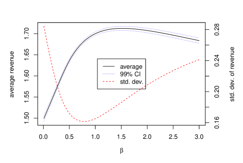
Figure 1: Average revenue and standard deviation of revenue for $T=5$

Three distinct phases can be identified in Fig. 1 from left to right. The first phase ($\beta<0.8$) witnesses increases in the average overall revenue with decreases in the standard deviation as $\beta$ increases, indicating that an overly conservative policy can not only hurt the revenue, but it may not really reduce the overall risk as supposed. To understand this apparent dilemma, note that the overall risk is different from the risk conditioned on historic prices: the former is estimated from runs that randomize all the prices, while the latter must fix the historic prices and only randomize the future prices. It is helpful to point out that more conservative policies with smaller $\beta$ values indeed have lower conditional risks. But for the overall risk at $\beta=0$, the policy trades everything in the first period at any price, while the policy at larger $\beta$ diversifies the risks by trading less at lower prices and reserves more for future opportunities, which not only increases expected revenue but also helps reduce the overall risk. The second phase ($0.8<\beta<1.5$) observes the normal case of increases in both revenue and overall risk. The third phase ($\beta>1.5$) experiences decreasing revenue while the risk increases. This is due to that an overly aggressive policy reserves too much quantity for the future and boldly takes the risk of selling a significant amount at whatever price in the last period.

This experiment provides some valuable insights, that both extreme conservatism ($\beta=0$) and extreme aggressiveness ($\beta\uparrow\infty$) give poor performance with low expected reward and high overall risk, and the ARM criterion may trade off and find a sweet spot in between. An overly conservative robust policy by the maximin reward criterion (i.e. $\beta=0$) can suffer both lower performance and higher overall risk. On the other hand, an overly aggressive robust policy for a big $\beta$ may also hurt the performance as it boldly exposes to future price risks by reserving too much inventory, ending up selling it in the last period at any price. Last but not least, there is a trade-off between the two extremes by adjusting the $\beta$ value of the ARM criterion. As illustrated in Figure 1, the fine-tuned $\beta$ may well go beyond $\beta=1$ for the minimax absolute regret criterion.

6 Conclusion.

This paper proposes the ARM criterion with the $\beta$ parameter for continuous control of conservatism. By minimizing the guarantee of worst-case regret against a $\beta$-adjusted benchmark that becomes more aggressive as $\beta$ increases, the ARM criterion chooses a solution that is likely to “mimic” the benchmark’s behavior, so that the conservatism of the recommended solution is moderated. Various theoretical properties of the ARM criterion are studied, such as continuity, monotonicity, and convexity, which may facilitate the analysis of problems, finding closed-form solutions, or designing better numerical algorithms to calculate competitive ratios. These theoretical investigations also lead to a new approach for competitive ratio analysis, which may be much simpler than the traditional approach for some problems, such as observed in the analysis of the one-way trading problem.

The tractability is studied for two-stage linear problems with the ARM criterion. Two particular situations are studied: the right-hand side uncertainty and the objective uncertainty. Equivalent reformulations into TSLRO/FR problems make it possible to take advantage of the tractable solution methods developed recently to solve them for practical applications.

Finally, the ARM criterion is applied to the robust one-way trading problem to demonstrate its properties and potential. Closed-form solutions are obtained, which facilitates the derivation of competitive ratios by the new approach. The optimal policy is shown to get more aggressive as the control parameter increases. A numerical study is carried out to demonstrate the effects of smooth control of conservatism for the one-way trading problem. Some insights are gleaned from the numerical study: extreme conservatism or aggressiveness may suffer from both lower average reward and higher overall risk at the same time, and the proper $\beta$ value is found somewhere in between.

The investigations of the ARM criterion carried out in this paper may serve as a starting point for future research. A rigorous analysis on how $\beta$ moderates conservatism is theoretically interesting and challenging at the same time. Conceivably, how to choose an appropriate $\beta$ value in real applications depends on the application context, and it is another worthy topic of interest for future study.

References

• Ardestani-Jaafari and Delage, (2016) Ardestani-Jaafari, A. and Delage, E. (2016). Robust optimization of sums of piecewise linear functions with application to inventory problems. Operations research, 64(2):474–494.
• Averbakh, (2005) Averbakh, I. (2005). Computing and minimizing the relative regret in combinatorial optimization with interval data. Discrete Optimization, 2(4):273–287.
• Averbakh and Lebedev, (2005) Averbakh, I. and Lebedev, V. (2005). On the complexity of minmax regret linear programming. European Journal of Operational Research, 160(1):227–231.
• Ben-Tal et al., (2009) Ben-Tal, A., El Ghaoui, L., and Nemirovski, A. (2009). Robust optimization. Princeton university press.
• Ben-Tal et al., (2004) Ben-Tal, A., Goryashko, A., Guslitzer, E., and Nemirovski, A. (2004). Adjustable robust solutions of uncertain linear programs. Mathematical programming, 99(2):351–376.
• Ben-Tal and Nemirovski, (1998) Ben-Tal, A. and Nemirovski, A. (1998). Robust convex optimization. Mathematics of operations research, 23(4):769–805.
• Ben-Tal and Nemirovski, (1999) Ben-Tal, A. and Nemirovski, A. (1999). Robust solutions of uncertain linear programs. Operations research letters, 25(1):1–13.
• Ben-Tal and Nemirovski, (2000) Ben-Tal, A. and Nemirovski, A. (2000). Robust solutions of linear programming problems contaminated with uncertain data. Mathematical programming, 88(3):411–424.
• Ben-Tal and Nemirovski, (2008) Ben-Tal, A. and Nemirovski, A. (2008). Selected topics in robust convex optimization. Mathematical Programming, 112(1):125–158.
• Bertsimas et al., (2011) Bertsimas, D., Brown, D. B., and Caramanis, C. (2011). Theory and applications of robust optimization. SIAM review, 53(3):464–501.
• Bertsimas et al., (2010) Bertsimas, D., Iancu, D. A., and Parrilo, P. A. (2010). Optimality of affine policies in multistage robust optimization. Mathematics of Operations Research, 35(2):363–394.
• Bertsimas and Sim, (2004) Bertsimas, D. and Sim, M. (2004). The price of robustness. Operations research, 52(1):35–53.
• Borodin and El-Yaniv, (2005) Borodin, A. and El-Yaniv, R. (2005). Online computation and competitive analysis. cambridge university press.
• Caldentey et al., (2017) Caldentey, R., Liu, Y., and Lobel, I. (2017). Intertemporal pricing under minimax regret. Operations Research, 65(1):104–129.
• Delage and Iancu, (2015) Delage, E. and Iancu, D. A. (2015). Robust multistage decision making. In The operations research revolution, pages 20–46. INFORMS.
• El-Ghaoui and Lebret, (1997) El-Ghaoui, L. and Lebret, H. (1997). Robust solutions to least-square problems to uncertain data matrices. Sima Journal on Matrix Analysis and Applications, 18:1035–1064.
• El Ghaoui et al., (1998) El Ghaoui, L., Oustry, F., and Lebret, H. (1998). Robust solutions to uncertain semidefinite programs. SIAM Journal on Optimization, 9(1):33–52.
• El-Yaniv et al., (2001) El-Yaniv, R., Fiat, A., Karp, R. M., and Turpin, G. (2001). Optimal search and one-way trading online algorithms. Algorithmica, 30(1):101–139.
• Gabrel et al., (2014) Gabrel, V., Murat, C., and Thiele, A. (2014). Recent advances in robust optimization: An overview. European journal of operational research, 235(3):471–483.
• Kouvelis and Yu, (2013) Kouvelis, P. and Yu, G. (2013). Robust discrete optimization and its applications, volume 14. Springer Science & Business Media.
• Lan et al., (2008) Lan, Y., Gao, H., Ball, M. O., and Karaesmen, I. (2008). Revenue management with limited demand information. Management Science, 54(9):1594–1609.
• Megiddo, (1978) Megiddo, N. (1978). Combinatorial optimization with rational objective functions. In Proceedings of the tenth annual ACM symposium on Theory of computing, pages 1–12.
• Milnor, (1951) Milnor, J. (1951). Games against nature. Technical report, RAND PROJECT AIR FORCE SANTA MONICA CA.
• Natarajan et al., (2014) Natarajan, K., Shi, D., and Toh, K.-C. (2014). A probabilistic model for minmax regret in combinatorial optimization. Operations Research, 62(1):160–181.
• Özkaya et al., (2022) Özkaya, M., İzgi, B., and Perc, M. (2022). Axioms of decision criteria for 3d matrix games and their applications. Mathematics, 10(23):4524.
• Perakis and Roels, (2008) Perakis, G. and Roels, G. (2008). Regret in the newsvendor model with partial information. Operations research, 56(1):188–203.
• Poursoltani and Delage, (2021) Poursoltani, M. and Delage, E. (2021). Adjustable robust optimization reformulations of two-stage worst-case regret minimization problems. Operations Research.
• Savage, (1951) Savage, L. J. (1951). The theory of statistical decision. Journal of the American Statistical association, 46(253):55–67.
• Shapiro, (2017) Shapiro, A. (2017). Interchangeability principle and dynamic equations in risk averse stochastic programming. Operations Research Letters, 45(4):377–381.
• Soyster, (1973) Soyster, A. L. (1973). Convex programming with set-inclusive constraints and applications to inexact linear programming. Operations research, 21(5):1154–1157.
• Stoye, (2011) Stoye, J. (2011). Statistical decisions under ambiguity. Theory and decision, 70(2):129–148.
• Vinod, (2021) Vinod, B. (2021). An approach to adaptive robust revenue management with continuous demand management in a covid-19 era. Journal of Revenue and Pricing management, 20(1):10–14.
• Wang et al., (2016) Wang, W., Wang, L., Lan, Y., and Zhang, J. X. (2016). Competitive difference analysis of the one-way trading problem with limited information. European Journal of Operational Research, 252(3):879–887.
• Yanıkoğlu et al., (2019) Yanıkoğlu, İ., Gorissen, B. L., and den Hertog, D. (2019). A survey of adjustable robust optimization. European Journal of Operational Research, 277(3):799–813.
• Zeng and Zhao, (2013) Zeng, B. and Zhao, L. (2013). Solving two-stage robust optimization problems using a column-and-constraint generation method. Operations Research Letters, 41(5):457–461.