SauvolaNet: Learning Adaptive Sauvola Network for Degraded Document Binarization

Abstract

Inspired by the classic Sauvola  local image thresholding approach, we systematically study it from the deep neural network (DNN) perspective and propose a new solution called SauvolaNet  for degraded document binarization (DDB). It is composed of three explainable modules, namely, Multi-Window Sauvola (MWS), Pixelwise Window Attention (PWA), and Adaptive Sauolva Threshold (AST). The MWS module honestly reflects the classic Sauvola  but with trainable parameters and multi-window settings. The PWA module estimates the preferred window sizes for each pixel location. The AST module further consolidates the outputs from MWS and PWA and predicts the final adaptive threshold for each pixel location. As a result, SauvolaNet  becomes end-to-end trainable and significantly reduces the number of required network parameters to 40K – it is only 1% of MobileNetV2. In the meantime, it achieves the State-of-The-Art (SoTA) performance for the DDB task – SauvolaNet  is at least comparable to, if not better than, SoTA binarization solutions in our extensive studies on the 13 public document binarization datasets. Our source code is available at https://github.com/Leedeng/SauvolaNet.

1 Introduction

Document binarization typically refers to the process of taking a gray-scale image and converting it to black-and-white. Formally, it seeks a decision function $f_{\textrm{binarize}}(\cdot)$ for a document image $\mathbf{D}$ of width $W$ and height $H$, such that the resulting image $\hat{\mathbf{B}}$ of the same size only contains binary values while the overall document readability is at least maintained if not enhanced.

$$\hat{\mathbf{B}}=f_{\textrm{binarize}}(\mathbf{D})$$ (1)

Document binarization plays a crucial role in many document analysis and recognition tasks. It is the prerequisite for many low-level tasks like connected component analysis, maximally stable extremal regions, and high-level tasks like text line detection, word spotting, and optical character recognition (OCR).

Instead of directly constructing the decision function $f_{\textrm{binarize}}(\cdot)$, classic binarization algorithms [17, 28] typically first construct an auxiliary function $g(\cdot)$ to estimate the required thresholds $\mathbf{T}$ as follows.

$$\mathbf{T}=g_{\textrm{classic}}(\mathbf{D})$$ (2)

In global thresholding approaches [17], this threshold $\mathbf{T}$ is a scalar, i.e. all pixel locations use the same threshold value. In contrast, this threshold $\mathbf{T}$ is a tensor with different values for different pixel locations in local thresholding approache [28]. Regardless of global or local thresholding, the actual binarization decision function can be written as

$$\hat{\mathbf{B}}_{\textrm{classic}}=f_{\textrm{classic}}(\mathbf{D})=th(\mathbf{D},\mathbf{T})=th(\mathbf{D},g_{\textrm{classic}}(\mathbf{D}))$$ (3)

where $th(x,y)$ is the simple thresholding function and the binary state for a pixel located at $i$-th row and $j$-th column is determined as in Eq. (4).

$$\hat{B}_{\textrm{classic}}[i,j]=th(D[i,j],T[i,j])=\begin{cases}+1,&\textrm{if\,}D[i,j]\geq T[i,j]\\ -1,&\textrm{otherwise}\end{cases}$$ (4)

Classic binarization algorithms are very efficient in general because of using simple heuristics like intensity histogram [17] and local contrast histogram [31]. The speed of classic binarization algorithms typical of the millisecond level, even on a mediocre CPU. However, simple heuristics also means that they are sensitive to potential variations [31] (image noise, illumination, bleed-through, paper materials, etc. ), especially when the relied heuristics fail to hold. In order to improve the binarization robustness, data-driven approaches like [33] learn the decision function $f_{\textrm{binarize}}(\cdot)$ from data rather than heuristics. However, these approaches typically achieve better robustness by using much more complicated features, and thus work relatively slow in practice, e.g. on the second level  [33].

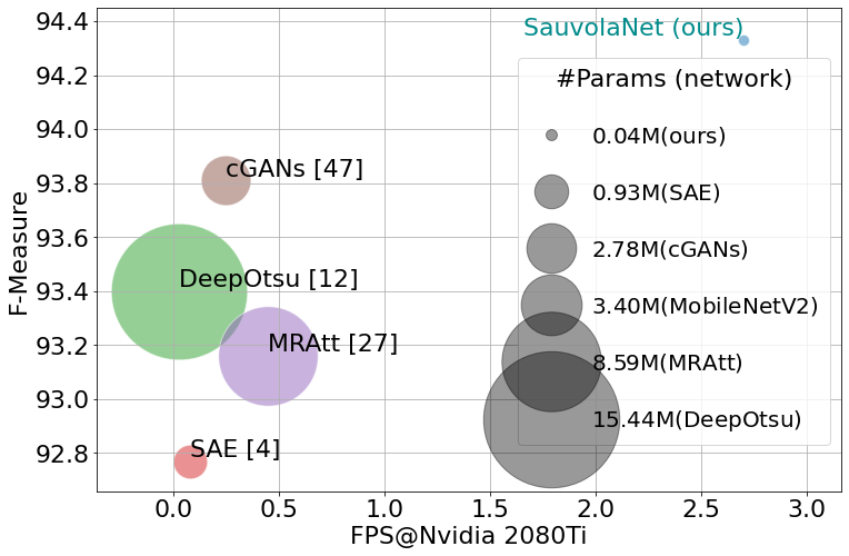
Figure 1: Comparisons of the SoTA DNN-based methods on the DIBCO 2011 dataset (average resolution 574$\times$1104). The SauvolaNet  is of 1% of MobileNetV2’s parameter size, while attaining superior performance in terms of both speed and F-Measure.

Like in many computer vision and image processing fields, the deep learning-based approaches outperform the classic approaches by a large margin in degraded document binarization tasks. The state-of-the-art (SoTA) binarization approaches are now all based on deep neural networks (DNN) [27, 22]. Most of SoTA document binarization approaches [2, 19, 32] treat the degraded binarization task as a binary semantic segmentation task (namely, foreground and background classes) or a sequence-to-sequence learning task [1], both of which can effectively learn $f_{\textrm{binarize}}(\cdot)$ as a DNN from data.

Recent efforts [2, 19, 9, 34, 5, 30, 32] focus more on improving robustness and generalizability. In particular, the SAE approach [2] suggests estimating the pixel memberships not from a DNN’s raw output but the DNN’s activation map, and thus generalizes well even for out-of-domain samples with a weak activation map. The MRAtt approach  [19] further improves the attention mechanism in multi-resolution analysis and enhances the DNN’s robustness to font sizes. DSN [32] apply multi-scale architecture to predict foreground pixel at multi-features levels. The DeepOtsu method [9] learns a DNN that iteratively enhances a degraded image to a uniform image and then binarized via the classic Otsu approach. Finally, generative adversarial networks (GAN) based approaches like cGANs [34] and DD-GAN [5] rely on the adversarial training to improve the model’s robustness against local noises by penalizing those problematic local pixel locations that the discriminator uses in differentiating real and fake results.

As one may notice, both classic and deep binarization approaches have pros and cons: 1) the classic binarization approaches are extremely fast, while the DNN solutions are not; 2) the DNN solutions can be end-to-end trainable, while the classic approaches can not. In this paper, we propose a novel document binarization solution called SauvolaNet  – it is an end-to-end trainable DNN solution but analogous to a multi-window Sauvola  algorithm. More precisely, we re-implement the Sauvola  idea as an algorithmic DNN layer, which helps SauvolaNet  attain highly effective feature representations at an extremely low cost – only two Sauvola  parameters are needed. We also introduce an attention mechanism to automatically estimate the required Sauvola  window sizes for each pixel location and thus could effectively and efficiently estimate the Sauvola  threshold. In this way, the SauvolaNet  significantly reduces the total number of DNN parameters to 40K, only 1% of the MobileNetV2, while attaining comparable performance of SoTA on public DIBCO datasets. Fig. 1 gives the high-level comparisons of the proposed SauvolaNet  to the SoTA DNN solutions.

The rest of the paper is organized as follows: Sec. 2 briefly reviews the classic Sauvola  method and its variants; Sec. 3 proposes the SauvolaNet solution for degraded document binarization; Sec. 4 presents Sauvola  ablation studies results and comparisons to SoTA methods; and we conclude the paper in Sec. 5.

2 Related Sauvola Approaches

The Sauvola  binarization algorithm [28] is widely used in main stream image and document processing libraries and systems like OpenCV  and Scikit-Image . As aforementioned, it constructs the binarization decision function (3) via the auxiliary threshold estimation function $g_{\textrm{Sauvola}}$, which has three hyper-parameters, namely, 1) $w$: the square window size (typically an odd positive integer [4]) for computing local intensity statistics; 2) $k$: the user estimated level of document degradation; and 3) $r$: the dynamic range of input image’s intensity variation.

$$\mathbf{T}_{\textrm{Sauvola}}=g_{\textrm{Sauvola}|\theta}(\mathbf{D}).$$ (5)

where $\theta\!\!=\!\!\{w,k,r\}$ indicates the used hyper-parameters. Each local threshold is computed w.r.t. the 1st- and 2nd-order intensity statistics as shown in Eq. (6),

$$T_{\textrm{Sauvola}|\theta}[i,j]=\mu[i,j]\cdot\left(1+k\cdot\left(\frac{\sigma[i,j]}{r}-1\right)\right)$$ (6)

where $\mu[i,j]$ and $\sigma[i,j]$ respectively indicate the mean and standard deviation of intensity values within the local window as follows.

$$\mu[i,j]=\sum_{\delta_{i}=-\lfloor w/2\rfloor}^{\lfloor w/2\rfloor}\sum_{\delta_{j}=-\lfloor w/2\rfloor}^{\lfloor w/2\rfloor}{D[i+\delta_{i},j+\delta_{j}]\over w^{2}}$$ (7)

$$\sigma^{2}[i,j]=\sum_{\delta_{i}=-\lfloor w/2\rfloor}^{\lfloor w/2\rfloor}\sum_{\delta_{j}=-\lfloor w/2\rfloor}^{\lfloor w/2\rfloor}{\left(D[i+\delta_{i},j+\delta_{j}]-\mu[i,j]\right)^{2}\over w^{2}}$$ (8)

It is well known that heuristic binarization methods with hyper-parameters could rarely achieve their upper-bound performance unless the method hyper-parameters are individually tuned for each input document image [12], and this is also the main pain point of Sauvola  approach.

Table 1: Comparisons of various Sauvola  document binarization approaches.

Related	End-to-End	Sauvola  Params.			#Used	Without
Work	Trainable?	$w$	$k$	$r$	Scales	Preproc?	Postproc?
Sauvola  [28]	✗	user specified			single	✓	✓
[14]	✗	auto	user specified	auto	multiple	✗	✗
[13]	✗	fixed			multiple	✓	✓
[8]	✗	fixed			single	✗	✗
[12]	✗	auto	fixed	fixed	multiple	✗	✓
SauvolaNet	✓	auto	learned	learned	multiple	✓	✓

Many efforts have been made to mitigate this pain point. For example, [14] introduces a multi-grid Sauvola  variant that analyzes multiple scales in the recursive way; [13] proposes a hyper-parameter free multi-scale binarization solution called Sauvola MS [2] by combining Sauvola  results of a fixed set of window sizes, each with its own empirical $k$ and $r$ values; [8] improves the classic Sauvola  by using contrast information obtained from pre-processing to refine Sauvola ’s binarization; [12] estimates the required window size $w$ in Sauvola  by using the stroke width transform matrix. Table 1 compares these approaches with the proposed SauvolaNet , and it is clear that only SauvolaNet  is end-to-end trainable.

3 The SauvolaNet Solution

Fig. 2 describes the proposed SauvolaNet  solution. It learns an auxiliary threshold estimation function from data by using a dual-branch design with three main modules, namely Multi-Window Sauvola (MWS), Pixelwise Window Attention (PWA), and Adaptive Sauvola Threshold (AST).

(a) The SauvolaNet  solution in training (i.e. $g_{Sauvola}(\cdot)$) and testing (i.e. $f_{\texttt{SauvolaNet}\,{}}(\cdot)$)
(b) Multi-Window Sauvola	(c) Pixel-wise Window Attention

Figure 2: The overview of SauvolaNet  solution and its trainable modules. $g_{\textrm{Sauvola}}$ and $g_{\textrm{SauvolaNet}}$ indicate the customized Sauvola  layer and SauvolaNet , respectively; Conv2D and AtrousConv2D indicate the traditional atrous (w/ dilation rate 2) convolution layers, respectively; each Conv2D/AtrousConv2D are denoted of format filters@ksize$\times$ksize and followed by InstanceNorm and ReLU layers; the last Conv2D in window attention uses the Softmax activation (denoted w/ borders); and Pixelwise Thresholding indicates the binarization process (4).

Specifically, the MWS module takes a gray-scale input image $\mathbf{D}$ and leverages on the Sauvola  to compute the local thresholds for different window sizes. The PSA module also takes $\mathbf{D}$ as the input but estimates the attentive window sizes for each pixel location. The AST module predicts the final threshold for each pixel location $\mathbf{T}$ by fusing the thresholds of different window sizes from MWS using the attentive weights from PWA. As a result, the proposed SauvolaNet  is analogous to a multi-window Sauvola , and models an auxiliary threshold estimation function $g_{\texttt{SauvolaNet}}$ between the input $\mathbf{D}$ and the output $\mathbf{T}$ as follows,

$$\mathbf{T}=g_{\texttt{SauvolaNet}}(\mathbf{D})$$ (9)

Unlike in the classic Sauvola ’s threshold estimation function (5), SauvolaNet  is end-to-end trainable and doesn’t require any hyper-parameter. Similar to Eq. (3), the binarization decision function $f_{\texttt{SauvolaNet}}$ used in testing as shown below

$$\hat{\mathbf{B}}=f_{\texttt{SauvolaNet}}(\mathbf{D})=th(\mathbf{D},\mathbf{T})=th(\mathbf{D},g_{\texttt{SauvolaNet}}(\mathbf{D}))$$ (10)

and the extra thresholding process (i.e. (4)) is denoted as the Pixelwise Thresholding (PT) in Fig. 2. Details about these modules are discussed in later sections.

	Single-window Threshold	Binarized Result
(a) Input $\mathbf{D}$	(b1) $\mathbf{S}_{1}=g_{\texttt{Sauvola}|{w=7}}(\mathbf{D})$	(c1) $th(\mathbf{D},\mathbf{S}_{1})$
	(b2) $\mathbf{S}_{2}=g_{\texttt{Sauvola}|{w=15}}(\mathbf{D})$	(c2) $th(\mathbf{D},\mathbf{S}_{2})$
	(b3) $\mathbf{S}_{3}=g_{\texttt{Sauvola}|{w=23}}(\mathbf{D})$	(c3) $th(\mathbf{D},\mathbf{S}_{3})$
	(b4) $\mathbf{S}_{4}=g_{\texttt{Sauvola}|{w=31}}(\mathbf{D})$	(c4) $th(\mathbf{D},\mathbf{S}_{4})$
	(b5) $\mathbf{S}_{5}=g_{\texttt{Sauvola}|{w=39}}(\mathbf{D})$	(c5) $th(\mathbf{D},\mathbf{S}_{5})$
	(b6) $\mathbf{S}_{6}=g_{\texttt{Sauvola}|{w=47}}(\mathbf{D})$	(c6) $th(\mathbf{D},\mathbf{S}_{6})$
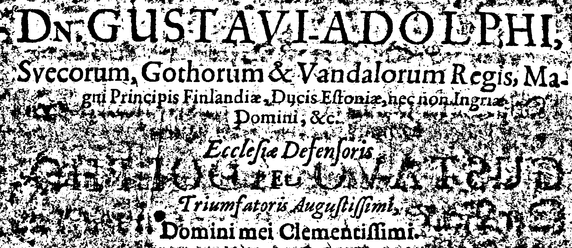
(d) GroundTruth	(b7) $\mathbf{S}_{7}=g_{\texttt{Sauvola}|{w=55}}(\mathbf{D})$	(c7) $th(\mathbf{D},\mathbf{S}_{7})$
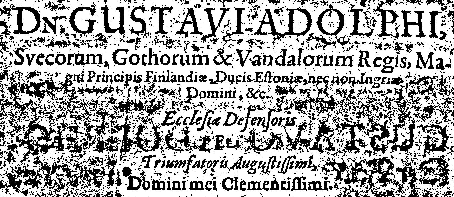
(e) Window attention	(b8) $\mathbf{S}_{8}=g_{\texttt{Sauvola}|{w=63}}(\mathbf{D})$	(c8) $th(\mathbf{D},\mathbf{S}_{8})$
(f) 5x enlarged red zone in (e)	(g) Adaptive Threshold $\mathbf{T}$	(h) Output $\hat{\mathbf{B}}=th(\mathbf{D},\mathbf{T})$

Figure 3: Intermediate results of SauvolaNet . Please note: 1) window attention (e) visualizes the most preferred window size of $\mathbf{A}$ for each pixel locations (i.e. $\operatorname{argmax}(\mathbf{A},\textrm{axis}=-1)$), and the 8 used colors correspond to those put before (b*); 2) binarized images (c*) are not used in SauvolaNet  but for visualization only; and 3) $g_{\textrm{Sauvola}}(\cdot)$ and $th(\cdot,\cdot)$ indicates the Sauvola layer and the pixelwise thresholding function (4), respectively.

3.1 Multi-Window Sauvola

The MWS module can be considered as a re-implementation of the classic multi-window Sauvola  analysis in the DNN context. More precisely, we first introduce a new DNN layer called Sauvola (denoted as $g_{\textrm{Sauvola}}(\cdot)$ in the function form), which has the Sauvola  window size as input argument and Sauvola ’s hyper-parameter $s$ and $r$ as trainable parameters. To enable multi-window analysis, we use a set of Sauvola layers, each corresponding to one window size in (11).The selection of window are verified in Sec. 4.2.

$$\mathbb{W}=\left\{w\,|\,w\in[7,15,23,31,39,47,55,63]\right\}$$ (11)

Fig. 3 visualizes all intermediate outputs of SauvolaNet , and Fig. 3-(b*) show predicted Sauvola  thresholds based on these window sizes, and Fig. 3-(c*) further binarize the input image using corresponding thresholds. These results again confirm that satisfactory binarization performance can be achieved by Sauvola  when the appropriate window size is used.

It is worthy to emphasize that Sauvola threshold computing window-wise mean and the standard deviation (see (6)) is very time-consuming when using the traditional DNN layers (e.g. , AveragePooling2D), especially for a big window size (e.g. , 31 or above). Fortunately, we implement our Sauvola layer by using integral image solution [29] to reduce the computational complexity to $O(1)$.

3.2 Pixelwise Window Attention

As mentioned in many works [13, 12], one disadvantage when using Sauvola  algorithm is the tuning of hyper-parameters. Among all three hyperparameters, namely, the window size $w$, the degradation level $k$, and the input deviation $r$, $w$ is the most important. Existing works typically decompose an input image into non-overlapping regions [18, 13] or grids [14] and apply each a different window size. However, existing solutions are not suitable for DNN implementation for two reasons: 1) non-overlapping decomposition is not a differentiable operation; and 2) processing regions/grids of different sizes are hard to parallelize.

Alternatively, we adopt the widely-accepted attention mechanism to remove the dependency on the user-specified window sizes. Specifically, the proposed PWA module is a sub-network that takes an input document image $\mathbf{D}$ and predicts the pixel-wise attention on all predefined window sizes. It conceptually follows the multi-grid method introduced by DeepLabv3 [3] while using a fixed dilation rate at 2. Also, we use the InstanceNormalization instead of the common BatchNormalization to mitigate the overfitting risk caused by a small training dataset. The detailed network architecture is shown in Fig. 2.

Sample result of PWA can be found in Fig. 3-(e). As one can see, the proposed PWA successfully predicts different window sizes for different pixels. More precisely, it prefers $w=39$ (see Fig. 3-(b5)) and $w=15$ (see Fig. 3-(b2)) for background and foreground pixels, respectively; and uses very large window sizes, e.g. , $w=63$ (i.e. Fig. 3-(b8)) for those pixels on text borders.

3.3 Adaptive Sauvola Threshold

As one can see from Fig. 2, the MWS outputs a Sauvola tensor $\mathbf{S}$ of size $H\times W\times N$, where $N$ is the number of used window sizes (and we use $N=8$, see Eq. (11)), the PWA outputs an attention tensor $\mathbf{A}$ of the same size as $\mathbf{S}$ and the attention sum for all window sizes on each pixel location is always 1, namely,

$$\sum_{k=1}^{N}A[i,j,k]=1,\,\,\forall 1\leq i\leq H,1\leq j\leq W.$$ (12)

The AST applies the window attention tensor $\mathbf{A}$ to the window-wise initial Sauvola threshold tensor $\mathbf{S}$ and compute the pixel-wise threshold $\mathbf{T}$ as below

$$T[i,j]=\sum_{k=1}^{N}A[i,j,k]\cdot S[i,j,k]$$ (13)

Fig. 3-(g) shows the adaptive threshold $\mathbf{T}$ when using the sample input Fig. 3-(a). By comparing the corresponding binarized result (i.e. Fig. 3-(h)) with those of single window’s results (i.e. Fig. 3-(c*)), one can easily verify that the adaptive threshold $\mathbf{T}$ outperforms any individual threshold result in $\mathbf{S}$.

3.4 Training, Inference, and Discussions

In order to train SauvolaNet , we normalize the input $\mathbf{D}$ to the range of (0,1) (by dividing 255 for uint8 image), and employ a modified hinge loss, namely

$$loss[i,j]=\max(1-\alpha\cdot(D[i,j]-T[i,j])\cdot B[i,j],0)$$ (14)

where $\mathbf{B}$ is the corresponding binarization ground truth map with binary values -1 (foreground) and +1 (background); $\mathbf{T}$ is SauvolaNet ’s predicted thresholds as shown in Eq. (9); and $\alpha$ is a parameter to empirically control the margin of decision boundary and only those pixels close to the decision boundary will be used in gradient back-propagation. Throughout the paper, we always use $\alpha=16$.

We implement SauvolaNet  in the TensorFlow framework. The used training patch size is 256$\times$256, and the data augmentations are random crop and random flip. The training batch size is set to 32, and we use Adam optimizer with the initial learning rate of 1$e$-3. During inference, we use $f_{\texttt{SauvolaNet}}$ instead of $g_{\texttt{SauvolaNet}}$ as shown in Fig. 2-(a). It only differs from the training in terms of one extra the thresholding step (4) to compare SauvolaNet  predicted thresholds with the original input to obtain the final binarized output.

Unlike in most DNNs, each module in SauvolaNet  is explainable: the MWS module leverages the Sauvola  algorithm to reduce the number of required network parameters significantly, and the PWA module employs the attention idea to get rid of the Sauvola ’s disadvantage of window size selection, and finally two branches are fused in the AST module to predict the pixel-wise threshold. Sample results in Fig. 3 further confirm that these modules work as expected.

4 Experimental Results

4.1 Dataset and Metrics

In total, 13 document binarization datasets are used in experiments, and they are {(H-)DIBCO 2009 [7] (10), 2010 [23] (10), 2011 [20] (16), 2012 [24] (14), 2013 [25] (16), 2014 [16] (10), 2016 [26] (10), 2017 [27] (20), 2018 [21] (10); PHIDB [15] (15), Bickely-diary dataset [6] (7), Synchromedia Multispectral dataset [10] (31), and Monk Cuper Set [9] (25)}. The braced numbers after each dataset indicates its sample size, and detailed partitions for training and testing will be specified in each study. For evaluation, we adopt the DIBCO metrics [20, 24, 25, 16, 26, 27, 21] namely, F-Measure (FM), psedudo F-Measure ($F_{ps}$), Distance Reciprocal Distortion metric (DRD) and Peak Signal-to-Noise Ratio (PSNR).

4.2 Ablation studies

To simplify discussion, let $\theta$ be the set of parameter settings related to a studied Sauvola  approach $f$. Unless otherwise noted, we always repeat a study about $f$ and $\theta$ on all datasets in the leave-one-out manner. More precisely, each score reported in ablation studies is obtained as follows

$$score(\theta,f)={1\over\|\mathbb{D}\|}\sum_{x\in\mathbb{X}}\left\{\sum_{(\mathbf{D},\mathbf{B})\in x}{m(\hat{\mathbf{B}}^{x}_{\theta},\mathbf{B})\over\|x\|}\right\}$$ (15)

where $m(\cdot)$ indicates a binarization metric, e.g. FM; and $\hat{\mathbf{B}}^{x}_{\theta}=f^{\mathbb{X}-x}_{\theta}(\mathbf{D})$ indicates the predicted binarized result for a given image $\mathbf{D}$ using the solution $f^{\mathbb{X}-x}_{\theta}$ that is trained on dataset ${\mathbb{X}-x}$ using the setting $\theta$. More precisely, the inner summation of Eq. (15) represents the average score for the model $f_{\theta}^{\mathbb{X}-x}$ over all testing samples in $x$, and that the outer summation of Eq. (15) further aggregates all leave-one-out average scores, and thus leaves the resulting score only dependent on the used method $f$ with setting $\theta$.

4.2.1 Does Sauvola  With Learnable Parameters Work Better?

Table 2: Trainable v.s. non-trainable Sauvola .

WinSize	Train?		Converged Value		Binarization Scores
$w$	$k$	$r$	$k$	$r$	FM(%)$\uparrow$	$F_{ps}$(%)$\uparrow$	PSNR(db)$\uparrow$	DRD$\downarrow$
OpenCV Parameter Configuration
11	✗	✗	0.50	0.50	50.09	59.95	13.44	13.73
	✗	✓	0.50	0.23 $\pm$ 0.003	77.31	81.25	15.86	8.17
	✓	✗	0.20 $\pm$ 0.005	0.50	77.92	85.44	15.99	8.09
	✓	✓	0.25 $\pm$ 0.024	0.24 $\pm$ 0.004	80.47	85.49	16.05	8.01
Pythreshold Parameter Configuration
15	✗	✗	0.35	0.50	67.37	76.83	14.84	9.96
	✗	✓	0.35	0.26 $\pm$ 0.004	79.23	84.01	15.72	8.71
	✓	✗	0.22 $\pm$ 0.011	0.50	79.87	86.31	15.84	8.17
	✓	✓	0.29 $\pm$ 0.027	0.28 $\pm$ 0.009	81.40	86.41	16.35	7.50
Scikit-Image Parameter Configuration
15	✗	✗	0.20	0.50	77.23	85.15	15.55	8.92
	✗	✓	0.20	0.25 $\pm$ 0.003	79.51	85.34	15.67	8.43
	✓	✗	0.22 $\pm$ 0.008	0.50	79.94	86.37	15.92	8.10
	✓	✓	0.29 $\pm$ 0.023	0.28 $\pm$ 0.007	81.46	86.47	16.38	7.46

Before discussing SauvolaNet , one must-answer question is whether or not re-implement the classic Sauvola  algorithm as an algorithmic DNN layer is the right choice, or equivalently, whether or not Sauvola  hyper-parameters learned from data could generalize better in practice. If not, we should leverage on existing heuristic Sauvola  parameter settings and use them in SauvolaNet  as non-trainable.

To answer the question, we start from one set of Sauvola  hyper-parameters, i.e. $\theta=\{w,k,r\}$, and evaluate the corresponding performance of single window Sauvola , i.e. $g_{\textrm{Sauvola}|\theta}$ under four different conditions, namely, 1) non-trainable $k$ and $r$; 2) non-trainable $k$ but trainable $r$; 3) trainable $k$ but non-trainable $r$; and 4) trainable $k$ and $r$. We further repeat the same experiments for three well-known Sauvola  hyper-parameter settings OpenCV($w$=11, $k$=0.5, $r$=0.5), Scikit-Image($w$=15, $k$=0.2, $r$=0.5) and Pythreshold ($w$=15, $k$=0.35, $r$=0.5).

Table 2 summarizes the performance scores for single-window Sauvola  with different parameter settings. Each row is about one $score(\theta,f_{\textrm{Sauvola}})$, and the three mega rows represent the three initial $\theta$ settings. As one can see, three prominent trends are: 1) the heuristic Sauvola  hyper-parameters (i.e. the non-trainable $k$ and $r$ setting) from the three open-sourced libraries don’t work well for DIBCO-like dataset; 2) allowing trainable $k$ or $r$ leads to better performance, and allowing both trainable gives even better performance; 3) the converged values of trainable $k$ and $r$ are different for different window sizes. We therefore use trainable $k$ and $r$ for each window size in the Sauvola layer (see Sec. 3.1).

4.2.2 Does Multiple-Window Help?

Though it seems that having multiple window sizes for Sauvola  analysis is beneficial, it is still unclear that 1) how effective it is comparing to a single-window Sauvola , and 2) what window sizes should be used. We, therefore, conduct ablation studies to answer both questions.

More precisely, we first conduct the leave-one-out experiments for the single-window Sauvola  algorithms for different window sizes with trainable $k$ and $r$. The resulting $score(w,f_{\textrm{Sauvola}})$ are presented in the upper-half of Table 3. Comparing to the best heuristic Sauvola  performance attained by Scikit-Image in Table 2, these results again confirm that Sauvola  with trainable $k$ and $r$ works much better. Furthermore, it is clear that $f_{\textrm{Sauvola}}$ with different window sizes (except for $w=7$) attain similar scores, possibly because there is no single dominant font size in the 13 public datasets.

Table 3: Ablation study on Sauvola  window sizes

WinSize								Binarization Scores
7	15	23	31	39	47	55	63	FM (%) $\uparrow$	$F_{ps}$ (%) $\uparrow$	PSNR (db) $\uparrow$	DRD $\downarrow$
Single-window Sauvola
✓								77.62	79.60	15.36	9.76
	✓							81.47	86.51	16.41	7.47
		✓						82.51	87.29	16.43	7.70
			✓					82.41	57.09	16.39	7.82
				✓				82.23	86.90	16.34	7.93
					✓			82.10	86.68	16.30	8.11
						✓		82.01	86.54	16.28	8.17
							✓	81.92	86.42	16.25	8.25
Multi-window Sauvola
✓	✓							81.55	84.41	17.09	6.62
✓	✓	✓						82.88	85.29	17.32	6.41
✓	✓	✓	✓					84.71	87.34	17.72	6.04
✓	✓	✓	✓	✓				87.83	90.70	18.47	5.30
✓	✓	✓	✓	✓	✓			89.87	92.31	18.87	4.13
✓	✓	✓	✓	✓	✓	✓		91.36	95.55	19.09	3.73
✓	✓	✓	✓	✓	✓	✓	✓	91.42	95.67	19.15	3.67

Finally, we conduct the ablation studies of using multiple window sizes in SauvolaNet  in the incremental way, and report the resulting $score(\mathbb{W},f_{\texttt{SauvolaNet}})$s in the lower-half of Table 3. It is now clear that 1) multi-window does help in SauvolaNet ; and 2) the more window sizes, the better performance scores. As a result, we use all eight window sizes in SauvolaNet  (see Eq. (11)).

4.3 Comparisons to Classic and SoTA Binarization Approaches

It is worthy to emphasize that different works [19, 9, 2, 34, 11, 13] use different protocols for document binarization evaluation. In this section, we mainly follow the evaluation protocol used in [9], and its dataset partitions are: 1) training: (H)-DIBCO 2009 [7], 2010 [23], 2012 [24]; Bickely-diary dataset [6]; and Synchromedia Multispectral dataset [10], and for testing: (H)-DIBCO 2011 [20], 2014 [16], and 2016 [26]. We train all approaches using the same evaluation protocol for fairly comparison. As a result, we focus on those recent and open-sourced DNN based methods, and they are SAE [2], DeepOtsu [9], cGANs [34] and MRAtt [19]. In addition, heuristic document binarization approaches Otsu [17], Sauvola [28] and Howe [11] are also included. Finally, Sauvola MS [13], a classic multi-window Sauvola solution is evaluated to better gauge the performance improvement from the heuristic multi-window analysis to the proposed learnable analysis.

Table 4: Comparison of SauvolaNet and SoTA approaches DIBCO 2011.

Dataset	Methods	FM (%) $\uparrow$	$F_{ps}$ (%) $\uparrow$	PSNR (db) $\uparrow$	DRD $\downarrow$
DIBCO 2011	Otsu [17]	82.10	84.80	15.70	9.00
	Howe [11]	91.70	92.00	19.30	3.40
	MRAtt [19]	93.16	95.23	19.78	2.20
	DeepOtsu [9]	93.40	95.80	19.90	1.90
	SAE [2]	92.77	95.68	19.55	2.52
	DSN [32]	93.30	96.40	20.10	2.00
	cGANs [34]	93.81	95.26	20.30	1.82
	Sauvola [28]	82.10	87.70	15.60	8.50
	Sauvola MS [13]	79.70	81.78	14.91	11.67
	SauvolaNet	94.32	96.40	20.55	1.97

Table 5: Comparison of SauvolaNet and SoTA approaches in H-DIBCO 2014.

Dataset	Methods	FM (%) $\uparrow$	$F_{ps}$ (%) $\uparrow$	PSNR (db) $\uparrow$	DRD $\downarrow$
H-DIBCO 2014	Otsu [17]	91.70	95.70	18.70	2.70
	Howe [11]	96.50	97.40	22.20	1.10
	MRAtt [19]	94.90	95.98	21.09	1.85
	DeepOtsu [9]	95.90	97.20	22.10	0.90
	SAE [2]	95.81	96.78	21.26	1.00
	DSN [32]	96.70	97.60	23.20	0.70
	DD-GAN [5]	96.27	97.66	22.60	1.27
	cGANs [34]	96.41	97.55	22.12	1.07
	Sauvola [28]	84.70	87.80	17.80	2.60
	Sauvola MS [13]	85.83	86.83	17.81	4.88
	SauvolaNet	97.83	98.74	24.13	0.65

Table 6: Comparison of SauvolaNet and SoTA approaches DIBCO 2016.

Dataset	Methods	FM (%) $\uparrow$	$F_{ps}$ (%) $\uparrow$	PSNR (db) $\uparrow$	DRD $\downarrow$
DIBCO 2016	Otsu [17]	86.60	89.90	17.80	5.60
	Howe [11]	87.50	82.30	18.10	5.40
	MRAtt [19]	91.68	94.71	19.59	2.93
	DeepOtsu [9]	91.40	94.30	19.60	2.90
	SAE [2]	90.72	92.62	18.79	3.28
	DSN [32]	90.10	83.60	19.00	3.50
	DD-GAN [5]	89.98	85.23	18.83	3.61
	cGANs [34]	91.66	94.58	19.64	2.82
	Sauvola [28]	84.60	88.40	17.10	6.30
	Sauvola MS [13]	79.84	81.61	14.76	11.50
	SauvolaNet	90.25	95.26	18.97	3.51

Original	cGANs [34]	DeepOtsu [9]	MRAtt [19]	SauvolaNet
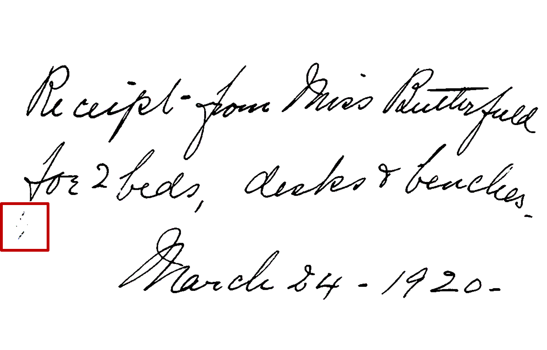
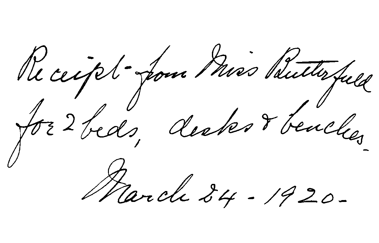
(a)	95.89	96.28	95.91	97.81
(b)	93.79	95.86	86.01	96.64
(c)	91.89	88.48	90.25	93.85
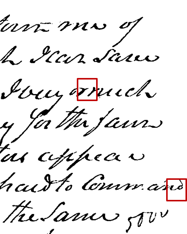
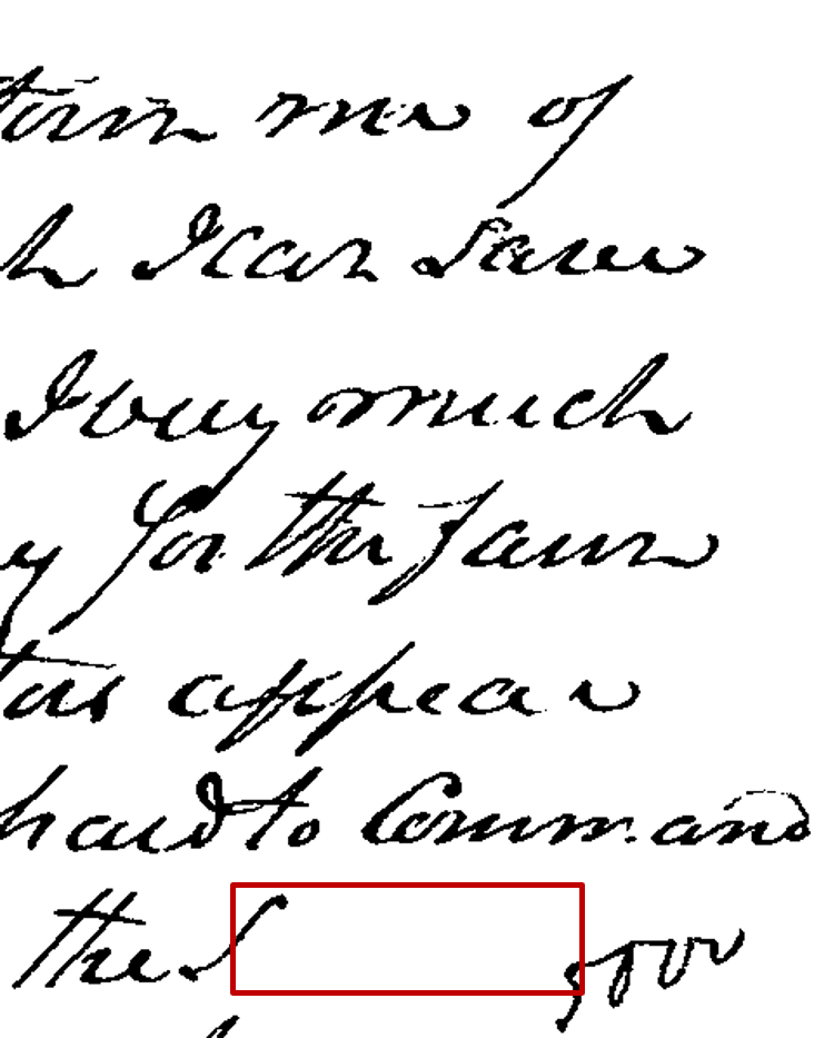
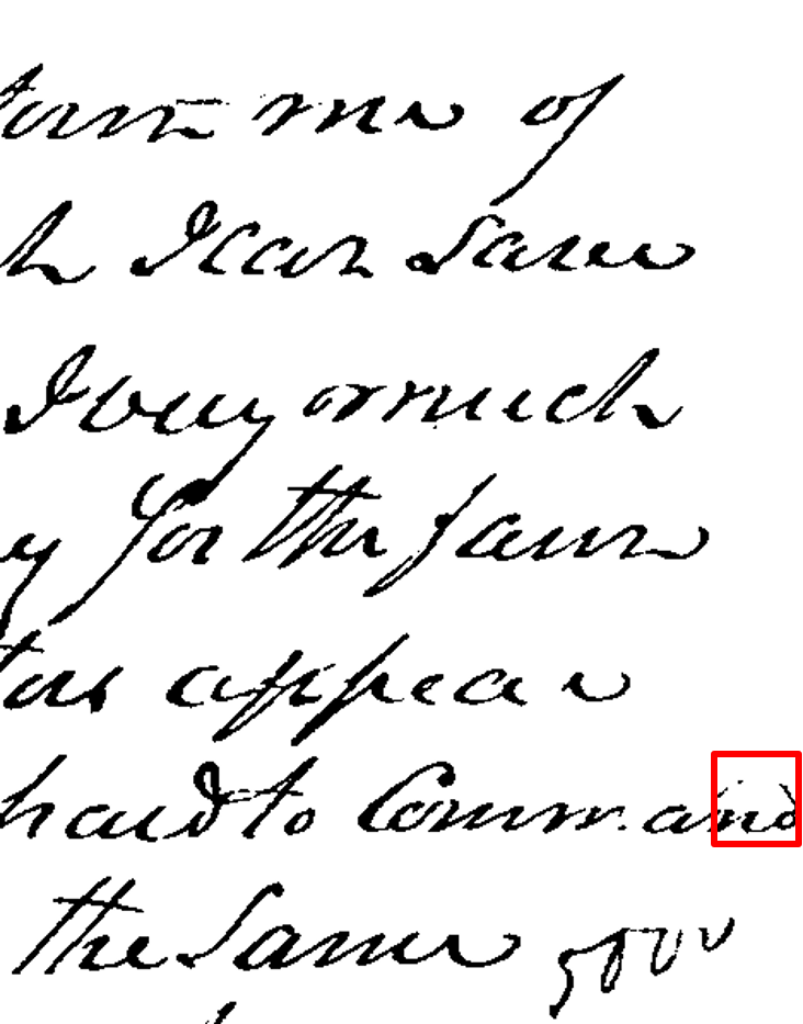
(d)	91.98	91.73	91.13	94.37

Figure 4: Qualitative comparison of SauvolaNet  with SoTA document binarization approaches. Problematic binarization regions are denoted in red boxes, and the FM score for each binarization result is also included below a result.

Table 4, 5 and 6 reports the average performance scores of the four evaluation metrics for all images in each testing dataset. When comparing the three Sauvola based approaches, namely, Sauvola, Sauvola MS, and SauvolaNet , one may easily notice that the heuristic multi-window solution Sauvola MS does not necessarily outperform the classic Sauvola. However, the SauvolaNet , again a multi-window solution but with all trainable weights, clearly beat both by large margins for all four evaluation metrics. Moreover, the proposed SauvolaNet  solution outperforms the rest of the classic and SoTA DNN approaches in DIBCO 2011. And SauvolaNet  is comparable to the SoTA solutions in H-DIBCO 2014 and DIBCO 2016. Sample results are shown in Fig. 4. More importantly, the SauvolaNet  is super lightweight and only contains 40K parameters. It is much smaller and runs much faster than other DNN solutions as shown in Fig. 1.

5 Conclusion

In this paper, we systematically studied the classic Sauvola  document binarization algorithm from the deep learning perspective and proposed a multi-window Sauvola  solution called SauvolaNet . Our ablation studies showed that the Sauvola  algorithm with learnable parameters from data significantly outperforms various heuristic parameter settings (see Table 2). Furthermore, we proposed the SauvolaNet  solution, a Sauvola -based DNN with all trainable parameters. The experimental result confirmed that this end-to-end solution attains consistently better binarization performance than non-trainable ones, and that the multi-window Sauvola  idea works even better in the DNN context with the help of attention (see Table 3). Finally, we compared the proposed SauvolaNet  with the SoTA methods on three public document binarization datasets. The result showed that SauvolaNet  has achieved or surpassed the SoTA performance while using a significantly fewer number of parameters (1% of MobileNetV2) and running at least 5x faster than SoTA DNN-based approaches.

References

- [1] Afzal, M.Z., Pastor-Pellicer, J., Shafait, F., Breuel, T.M., Dengel, A., Liwicki, M.: Document image binarization using lstm: A sequence learning approach. In: Int. workshop on historical document Imag. and Process. pp. 79–84 (2015)
- [2] Calvo-Zaragoza, J., Gallego, A.J.: A selectional auto-encoder approach for document image binarization. Pattern Recognit. 86, 37–47 (2019)
- [3] Chen, L.C., Papandreou, G., Schroff, F., Adam, H.: Rethinking atrous convolution for semantic image segmentation. arXiv preprint arXiv:1706.05587 (2017)
- [4] Cheriet, M., Moghaddam, R.F., Hedjam, R.: A learning framework for the optimization and automation of document binarization methods. Comput. Vis. Image Underst. 117(3), 269–280 (2013)
- [5] De, R., Chakraborty, A., Sarkar, R.: Document image binarization using dual discriminator generative adversarial networks. IEEE Signal Process. Lett. 27, 1090–1094 (2020)
- [6] Deng, F., Wu, Z., Lu, Z., Brown, M.S.: Binarizationshop: a user-assisted software suite for converting old documents to black-and-white. In: Proceedings of the 10th annual joint Conf. on Digital libraries. pp. 255–258 (2010)
- [7] Gatos, B., Ntirogiannis, K., Pratikakis, I.: ICDAR 2009 document image binarization contest (DIBCO 2009). In: Int. Conf. on document Anal. and Recognit. pp. 1375–1382. IEEE (2009)
- [8] Hadjadj, Z., Meziane, A., Cherfa, Y., Cheriet, M., Setitra, I.: Isauvola: Improved sauvola’s algorithm for document image binarization. In: Int. Conf. on Image Anal. and Recognit. pp. 737–745. Springer (2016)
- [9] He, S., Schomaker, L.: Deepotsu: Document enhancement and binarization using iterative deep learning. Pattern Recognit. 91, 379–390 (2019)
- [10] Hedjam, R., Nafchi, H.Z., Moghaddam, R.F., Kalacska, M., Cheriet, M.: ICDAR 2015 contest on multispectral text extraction (ms-tex 2015). In: Int. Conf. on Document Anal. and Recognit. pp. 1181–1185. IEEE (2015)
- [11] Howe, N.R.: Document binarization with automatic parameter tuning. Int. J. Doc. Anal. Recognit. 16(3), 247–258 (2013)
- [12] Kaur, A., Rani, U., Josan, G.S.: Modified sauvola binarization for degraded document images. Eng. Appl. Artif. Intell. 92, 103672 (2020)
- [13] Lazzara, G., Géraud, T.: Efficient multiscale sauvola’s binarization. Int. J. Doc. Anal. Recognit. 17(2), 105–123 (2014)
- [14] Moghaddam, R.F., Cheriet, M.: A multi-scale framework for adaptive binarization of degraded document images. Pattern Recognit. 43(6), 2186–2198 (2010)
- [15] Nafchi, H.Z., Ayatollahi, S.M., Moghaddam, R.F., Cheriet, M.: An efficient ground truthing tool for binarization of historical manuscripts. In: Int. Conf. on Document Anal. and Recognit. pp. 807–811. IEEE (2013)
- [16] Ntirogiannis, K., Gatos, B., Pratikakis, I.: ICFHR2014 competition on handwritten document image binarization (H-DIBCO 2014). In: Int. Conf. on frontiers in handwriting Recognit. pp. 809–813. IEEE (2014)
- [17] Otsu, N.: A threshold selection method from gray-level histograms. IEEE Trans. Syst. Man Cybern. 9(1), 62–66 (1979)
- [18] Pai, Y.T., Chang, Y.F., Ruan, S.J.: Adaptive thresholding algorithm: Efficient computation technique based on intelligent block detection for degraded document images. Pattern Recognit. 43(9), 3177–3187 (2010)
- [19] Peng, X., Wang, C., Cao, H.: Document binarization via multi-resolutional attention model with drd loss. In: Int. Conf. on Document Anal. and Recognit. pp. 45–50. IEEE (2019)
- [20] Pratikakis, I., Gatos, B., Ntirogiannis, K.: ICDAR 2011 document image binarization contest (DIBCO 2011). In: Int. Conf. on Document Anal. and Recognit. pp. 1506–1510 (2011)
- [21] Pratikakis, I., Zagori, K., Kaddas, P., Gatos, B.: ICFHR 2018 competition on handwritten document image binarization (H-DIBCO 2018). In: Int. Conf. on Frontiers in Handwriting Recognit. pp. 489–493 (2018)
- [22] Pratikakis, I., Zagoris, K., Karagiannis, X., Tsochatzidis, L., Mondal, T., Marthot-Santaniello, I.: Icdar 2019 competition on document image binarization (dibco 2019). In: Int. Conf. on Document Anal. and Recognit. pp. 1547–1556 (2019)
- [23] Pratikakis, I., Gatos, B., Ntirogiannis, K.: H-DIBCO 2010-handwritten document image binarization competition. In: Int. Conf. on Frontiers in Handwriting Recognit. pp. 727–732. IEEE (2010)
- [24] Pratikakis, I., Gatos, B., Ntirogiannis, K.: ICFHR 2012 competition on handwritten document image binarization (H-DIBCO 2012). In: Int. Conf. on frontiers in handwriting Recognit. pp. 817–822. IEEE (2012)
- [25] Pratikakis, I., Gatos, B., Ntirogiannis, K.: ICDAR 2013 document image binarization contest (DIBCO 2013). In: Int. Conf. on Document Anal. and Recognit. pp. 1471–1476. IEEE (2013)
- [26] Pratikakis, I., Zagoris, K., Barlas, G., Gatos, B.: ICFHR2016 handwritten document image binarization contest (H-DIBCO 2016). In: Int. Conf. on Frontiers in Handwriting Recognit. pp. 619–623. IEEE (2016)
- [27] Pratikakis, I., Zagoris, K., Barlas, G., Gatos, B.: ICDAR2017 competition on document image binarization (DIBCO 2017). In: Int. Conf. on Document Anal. and Recognit. vol. 1, pp. 1395–1403. IEEE (2017)
- [28] Sauvola, J., Pietikäinen, M.: Adaptive document image binarization. Pattern Recognit. 33(2), 225–236 (2000)
- [29] Shafait, F., Keysers, D., Breuel, T.M.: Efficient implementation of local adaptive thresholding techniques using integral images. In: Document recognition and retrieval XV. vol. 6815, p. 681510. Int. Society for Optics and Photonics (2008)
- [30] Souibgui, M.A., Kessentini, Y.: De-gan: A conditional generative adversarial network for document enhancement. IEEE Trans. Pattern Anal. Mach. Intell. (2020)
- [31] Su, B., Lu, S., Tan, C.L.: Robust document image binarization technique for degraded document images. IEEE Trans. Image Process. 22(4), 1408–1417 (2012)
- [32] Vo, Q.N., Kim, S.H., Yang, H.J., Lee, G.: Binarization of degraded document images based on hierarchical deep supervised network. Pattern Recognit. 74, 568–586 (2018)
- [33] Wu, Y., Natarajan, P., Rawls, S., AbdAlmageed, W.: Learning document image binarization from data. In: Int. Conf. on Image Process. pp. 3763–3767 (2016)
- [34] Zhao, J., Shi, C., Jia, F., Wang, Y., Xiao, B.: Document image binarization with cascaded generators of conditional generative adversarial networks. Pattern Recognit. 96, 106968 (2019)