Bayesian variational regularization on the ball

Abstract

We develop variational regularization methods which leverage sparsity-promoting priors to solve severely ill-posed inverse problems defined on the 3D ball (i.e. the solid sphere). Our method solves the problem natively on the ball and thus does not suffer from discontinuities that plague alternate approaches where each spherical shell is considered independently. Additionally, we leverage advances in probability density theory to produce Bayesian variational methods which benefit from the computational efficiency of advanced convex optimization algorithms, whilst supporting principled uncertainty quantification. We showcase these variational regularization and uncertainty quantification techniques on an illustrative example. The C++ code discussed throughout is provided under a GNU general public license.

I Introduction

Inverse problems on Euclidean manifolds have been researched extensively and associated techniques have found effective application in countless domains. However, increasingly often one wishes to consider inverse problems defined on curved, non-Euclidean manifolds, e.g. diffusion magnetic resonance imaging (MRI) [1] and 2D dark matter reconstructions on the sphere, and many aspects of geophysics [2, 3, 4], astrophysics [5, 6], and molecular modeling [7] on the 3D ball, for which very few techniques have been developed.

Inverse problems are often solved by Bayesian Markov chain Monte Carlo (MCMC) sampling methods or variational approaches (optimization etc.). MCMC methods are highly computationally demanding on the ball, due to the computational complexity of transforms on curved manifolds, and are infeasible for many applications. Variational methods, which solve inverse problems through classical optimization techniques, are typically scalable and robust, supporting both theoretical guarantees, and can support principled uncertainty quantification (as demonstrated in this letter). Such techniques are thus perfectly suited to scientific analysis on the ball, where computational efficiency and probabilistic interpretations are highly desirable. Variational methods have been considered over the sphere [8, 9, 10], often leveraging ideas from compressed sensing [11, 12], and typically promoting sparsity in spherical wavelet dictionaries, e.g. [13, 14, 15], to recover state-of-the-art results. Spherical techniques have been used tomographically (as concentric spherical shells) to model radially distributed datasets, however holistic approaches, which perform analysis natively on the underlying manifold (the ball), are crucially missing. Wavelet transforms on the 3D ball have been developed to support radially distributed problems [16, 17, 18, 19, 20, 21], however these dictionaries have, to our best knowledge, not been leveraged to perform variational inference on the ball.

In this letter we develop scalable techniques, with associated open-source software, which leverage variational regularization methods to solve ill-posed and/or ill-conditioned inverse problems natively on the ball. Furthermore, leveraging recent developments in the theory of probability density theory [22], we demonstrate how convex variational regularization techniques can be combined with advances in probability density theory to construct computationally efficient signal reconstruction techniques on the ball with principled uncertainty quantification, or ‘Bayesian variational regularization’.

II Bayesian variational regularization on ball

In this section we develop mathematical techniques for the analysis of spin signals on the 3D ball and wavelets on the directional ball, scalable convex optimization algorithms on the ball, and variational regularization techniques which support principled Bayesian uncertainty quantification. Throughout we adopt separable eigenfunctions on the ball, with radial basis functions given by the Laguerre polynomials [23, 24] and angular basis functions given by the spin spherical harmonics ${}_{s}Y_{\ell m}$ [25, 26, 27, 28]. As spin spherical harmonic transform are more common in the associated literature, we will focus primarily on the novel radial components [21], and the Bayesian interpretation [22, 29, 30, 31].

II-A Spin signals on the ball

Here we discuss the construction of Spherical-Laguerre basis functions on the 3D ball, developed in previous work [21] and adopted throughout this letter. First let us define the Laguerre basis functions along the radial half-line $K_{p}(r)$ as

$$K_{p}(r)\equiv\sqrt{\frac{p!}{(p+2)!}}\frac{e^{\frac{-r}{2\tau}}}{\sqrt{\tau^{3}}}L_{p}^{(2)}(\frac{r}{\tau}),$$ (1)

where $L_{p}^{(2)}$ is the $p^{\text{th}}$-associated $2^{\text{nd}}$-order Laguerre polynomial [23, 24], and $\tau\in\mathbb{R}^{+}$ is a scale factor that adds a scaling flexibility. These basis functions are orthonormal on $\mathbb{R}^{+}$, i.e. $\langle K_{p}|K_{q}\rangle_{\mathbb{R}^{+}}=\delta_{pq}$, and complete, by Gram-Schmidt orthogonalization and exploiting polynomial completeness on $\mathsf{L}^{2}(\mathbb{R}^{+},r^{2}e^{-r}\mathop{}\!\mathrm{d}r)$ [21]. Any square-integrable function $f\in\mathsf{L}^{2}(\mathbb{R}^{+})$ can be projected into this basis as

$$f_{p}=\langle f|K_{p}\rangle=\int_{\mathbb{R}^{+}}\mathop{}\!\mathrm{d}rr^{2}f(r)K_{p}(r),$$ (2)

which supports exact synthesis by

$$f(r)=\sum_{p=0}^{\infty}f_{p}K_{p}(r).$$ (3)

Real-world functions are typically to a good approximation bandlimited, i.e. the Fourier-Laguerre coefficients of signals $f\in\mathbb{R}^{+}$ are such that $f_{p}=0,\forall p\geq P$, and so this summation is truncated at $P$. We adopt the Gauss-Laguerre quadrature (see e.g. [32]), which is commonly used to numerically evaluate integrals over the radial half-line, and was used to develop an exact sampling theorem on Spherical-Laguerre space [21].

Suppose we adopt these radial basis functions which we then combine with the spin-$s$ spherical harmonic angular basis functions ${}_{s}Y_{\ell m}(\omega)$ [25, 26] for $s\in\mathbb{Z}$ and $\omega=(\theta,\psi)\in\mathbb{S}^{2}$, where $\theta=[0,\pi)$ is the colatitude and $\psi\in[0,2\pi)$ is the longitude. In such a case, we can straightforwardly define the Spherical-Laguerre basis functions ${}_{s}Z_{\ell mp}(\bm{r})=K_{p}(r)_{s}Y_{\ell m}(\omega)$ for $\bm{r}=(r,\omega)\in\mathbb{B}^{3}\coloneqq\mathbb{R}^{+}\times\mathbb{S}^{2}$, which are orthogonal $\langle_{s}Z_{\ell mp}|_{s}Z_{\ell^{\prime}m^{\prime}p^{\prime}}\rangle_{\mathbb{B}^{3}}=\delta_{\ell\ell^{\prime}}\delta_{mm^{\prime}}\delta_{pp^{\prime}}$ and onto which any square integrable spin-$s$ function on the ball ${}_{s}f\in\mathsf{L}^{2}(\mathbb{B}^{3})$ can be projected by

$${}_{s}f_{\ell mp}=\langle_{s}f|_{s}Z_{\ell mp}\rangle_{\mathbb{B}^{3}}=\int_{\mathbb{B}^{3}}\mathop{}\!\mathrm{d}\mu(\bm{r})_{s}f(\bm{r})_{s}Z_{\ell mp}^{*}(\bm{r}),$$ (4)

where $\mathop{}\!\mathrm{d}\mu(\bm{r})=\mathop{}\!\mathrm{d}^{3}\bm{r}=r^{2}\sin{\theta}\mathop{}\!\mathrm{d}r\mathop{}\!\mathrm{d}\theta\mathop{}\!\mathrm{d}\psi$ is the rotation invariant measure (Haar measure) on the ball. By considering the separability and completeness of angular and radial basis functions this projection supports exact synthesis, such that

$${}_{s}f(\bm{r})=\sum_{p=0}^{P-1}\sum_{\ell=0}^{L-1}\sum_{m=-\ell}^{\ell}{}_{s}f_{\ell mp}{}_{s}Z_{\ell mp}(\bm{r}),$$ (5)

where $L,P\in\mathbb{Z}^{+}$ are the angular [27] and radial [21] bandlimits respectively. In this work, by considering the relations presented in this subsection, fast adjoint Spherical-Laguerre transforms were constructed, facilitating variational regularization on the ball (see Section III).

II-B Directional scale-discretized wavelets on the ball

Here we extend the Spherical-Laguerre wavelets on the 3D ball developed in previous work [21] to 4D directional scale-discretized wavelets on the ball. Furthermore, we extend the discussion to include spin-signals, which arise in various areas of physics e.g. quantum mechanics and weak gravitational lensing [31]. Consider the radial translation operator $\scalerel*{\tau}{T}_{r}$ for $r\in\mathbb{R}^{+}$ (see [21, 33] for further details), and rotation $\mathcal{R}_{\rho}$, for Euler angles $\rho=(\alpha,\beta,\gamma)\in\text{SO}(3)$ with $\alpha\in[0,2\pi)$, $\beta\in[0,\pi)$, and $\gamma\in[0,2\pi)$, with action $(\mathcal{R}_{\rho}{}_{s}f)(\omega)\equiv e^{-is\theta}{}_{s}f(\mathcal{R}_{\rho}^{-1}\bm{\omega})$. Further define the concatenation of these transforms to be the 4D transformation $\mathcal{L}_{\bm{h}}=\scalerel*{\tau}{T}_{r}\mathcal{R}_{\rho}$ for $\bm{h}=(r,\rho)\in\mathbb{H}^{4}\coloneqq\mathbb{R}^{+}\times\text{SO}(3)$. Leveraging this composite transformation one can straightforwardly define the directional wavelet coefficients $W^{{}_{s}\Psi^{jj^{\prime}}}\in\mathsf{L}^{2}(\mathbb{H}^{4})$ of any square integrable spin-$s$ function ${}_{s}f\in\mathsf{L}^{2}[\mathbb{B}^{3}]$ by the directional convolution $\circledast$

$$W^{{}_{s}\Psi^{jj^{\prime}}}(\bm{h}) \equiv({}_{s}f\circledast{}_{s}\Psi^{jj^{\prime}})(\bm{h})\equiv\langle{}_{s}f,\mathcal{L}_{\bm{h}}{}_{s}\Psi^{jj^{\prime}}\rangle_{\mathbb{B}^{3}}$$

$$=\int_{\mathbb{B}^{3}}\mathop{}\!\mathrm{d}\mu(\bm{r}){}_{s}f(\bm{r})(\mathcal{L}_{\bm{h}}{}_{s}\Psi^{jj^{\prime}})^{\star}(\bm{r}),$$ (6)

where ${}_{s}\Psi^{jj^{\prime}}\in\mathsf{L}^{2}[\mathbb{B}^{3}]$ is the wavelet kernel at angular and radial scales $j,j^{\prime}\in\mathbb{Z}^{+}$ respectively. These scales determine the volume over which a given wavelet function has compact support [21]. Typically, wavelet coefficients do not capture low frequency signal content, which instead is captured by axisymmetric scaling functions ${}_{s}\Upsilon\in\mathsf{L}^{2}(\mathbb{B}^{3})$ with coefficients $W^{{}_{s}\Upsilon}\in\mathsf{L}^{2}(\mathbb{B}^{3})$ defined by the axisymmetric convolution $\odot$ with a spin-$s$ signal ${}_{s}f\in\mathsf{L}^{2}(\mathbb{B}^{3})$ such that

$$W^{{}_{s}\Upsilon}(\bm{r}) \equiv({}_{s}f\odot{}_{s}\Upsilon)(\bm{r})\equiv\langle{}_{s}f,\mathcal{L}_{\bm{r}}{}_{s}\Upsilon\rangle_{\mathbb{B}^{3}}$$

$$=\int_{\mathbb{B}^{3}}\mathop{}\!\mathrm{d}\mu(\bm{r}^{\prime}){}_{s}f(\bm{r}^{\prime})(\mathcal{L}_{\bm{r}}{}_{s}\Upsilon)^{\star}(\bm{r}^{\prime})\,,$$ (7)

where $\mathcal{L}_{\bm{r}}$ is an axisymmetric simplification of the full 4D transformation $\mathcal{L}_{\bm{h}}$. For suitable choices of wavelet and scaling generating functions (those which satisfy wavelet admissibility) these projections support exact synthesis by

$${}_{s}f(\bm{r}) =\int_{\mathbb{B}^{3}}\mathop{}\!\mathrm{d}\mu(\bm{r}^{\prime})W^{{}_{s}\Upsilon}(\bm{r}^{\prime})(\mathcal{L}_{\bm{r}^{\prime}}{}_{s}\Upsilon)(\bm{r})$$

$$+ \sum_{j=J_{0}}^{J}\sum_{j^{\prime}=J^{\prime}_{0}}^{J^{\prime}}\int_{\mathbb{H}^{4}}\mathop{}\!\mathrm{d}\mu(\bm{h})W^{{}_{s}\Psi^{jj^{\prime}}}(\bm{h})(\mathcal{L}_{\bm{h}}{}_{s}\Psi^{jj^{\prime}})(\bm{r}),$$ (8)

where $\mathop{}\!\mathrm{d}\mu(\bm{h})=\mathop{}\!\mathrm{d}^{4}\bm{h}=r^{2}\sin{\beta}\mathop{}\!\mathrm{d}r\mathop{}\!\mathrm{d}\alpha\mathop{}\!\mathrm{d}\beta\mathop{}\!\mathrm{d}\gamma$ is the Haar measure on $\mathbb{H}^{4}$. By construction [21] this wavelet dictionary exhibits both good frequency and spatial localization, permits exact synthesis, and leverages optimal sampling theories for efficient transforms. Furthermore, by adopting adjoint Spherical-Laguerre transforms (see subsection II-A) fast adjoint 4D wavelet transforms on the ball were constructed.

II-C Efficient transformations on the ball

Variational methods on the ball require an additional level of complexity over those defined on the spherical manifolds, which are already significantly computationally expensive. The forward and inverse Spherical-Laguerre transforms are computed through the FLAG package [21] with computational complexity $\sim\mathcal{O}(L^{4})$, built on spin spherical harmonic transforms provided by the SSHT package [27, 8]. Similarly, forward and inverse wavelets transforms on the 3D ball are computed through the FLAGLET package [21] with computational complexity $\sim\mathcal{O}(NL^{4})$, where $N\in\mathbb{Z}^{+}$ is the wavelet directionality, built on the wavelet transforms provided by the S2LET package [34, 14, 28, 15, 13, 35]. Both these transforms on the ball (FLAG and FLAGLET) scale at least quartically with bandlimit. Therefore, even optimally sampled transforms on the ball are very computationally expensive, motivating attention to scalable implementations.

II-D Bayesian variational regularization on the ball

Consider measurements $\bm{y}\in\mathbb{R}^{M}$, e.g. observations on the sky with some radial component, which may be related to some intrinsic underlying field of interest on the ball $\bm{x}\in\mathbb{R}^{N_{\mathbb{B}^{3}}}$ by a sensing operator $\bm{\mathsf{\Phi}}\in\mathbb{R}^{M\times N_{\mathbb{B}^{3}}}:\bm{x}\mapsto\bm{y}$. Further suppose measurements are polluted with noise $\bm{n}$, then our measurement model is generally given by $\bm{y}=\bm{\mathsf{\Phi}}\bm{x}+\bm{n}$, which is both classically ill-posed in the sense of Hadamard [36] and may be seriously ill-conditioned. There are many methods for inferring $\bm{x}$ from $\bm{y}$, in this work we will consider a Bayesian variational approach, so as to benefit from the computational efficiency of variational methods (a key component on the ball) whilst retaining the principled statistical interpretation provided by Bayesian methods.

In a Bayesian sense, given a sufficient understanding of our physical system (including e.g. the forward model and the noise distribution etc.) we can assign a likelihood distribution $P(\bm{y}|\bm{x};\bm{\mathsf{\Phi}})$, which acts as a data-fidelity constraint on our solutions. Furthermore, suppose we have some a priori knowledge as to the nature of our latent variable, e.g. $\bm{x}$ is presumed to be sparse in a given dictionary, then we can straightforwardly define a Bayesian prior distribution $P(\bm{x})$, which acts as a regularization functional to stabilize our inference. With these distributions defined we can construct our posterior distribution through Bayes’ theorem

$$P(\bm{x}|\bm{y};\bm{\mathsf{\Phi}})\propto P(\bm{y}|\bm{x};\bm{\mathsf{\Phi}})P(\bm{x}),$$ (9)

where we drop the normalization term (Bayesian evidence) as it does not affect our solution, and for simplicity. A reasonable choice of solution, in a Bayesian sense, is that which maximizes the posterior odds (i.e. the most likely one), called the maximum a posteriori (MAP) solution, given by

$$\bm{x}^{\text{MAP}} \equiv\operatorname*{argmax}_{\bm{x}}\big{\{}P(\bm{x}|\bm{y};\bm{\mathsf{\Phi}})\big{\}},$$

$$\propto\operatorname*{argmin}_{\bm{x}}\big{\{}-\log(\;P(\bm{y}|\bm{x};\bm{\mathsf{\Phi}})P(\bm{x})\;)\big{\}},$$

$$\propto\operatorname*{argmin}_{\bm{x}}\big{\{}h(\bm{x})=f(\bm{x})+g(\bm{x})\big{\}},$$ (10)

where the second line comes from the monotonicity of the logarithm function. The final line highlights that MAP estimation, for the common class of log-concave distributions, yields convex objectives $h(\bm{x})$, and this is equivalent to unconstrained convex optimization. Such optimization problems typically leverage $1^{\text{st}}$-order information to efficiently converge to global (from convexity) extremal solutions [37]. For convex but non-differentiable objectives (e.g. sparsity priors) gradient information is accessed through the proximal projection [38], and thus extremal solutions are efficiently recovered via proximal optimization algorithms [39, 37]. Such algorithms permit strong guarantees of both convergence and rate of convergence, however they still only recover point estimates and do not naively support uncertainty quantification.

II-E Uncertainty quantification of MAP estimation

Bayesian methods often consider credible regions (regions of high probability concentration) $C_{\alpha}\subset\mathbb{C}^{N_{\mathbb{B}^{3}}}$ of the full posterior distribution, at $100(1-\alpha)\%$ confidence, by evaluating

$$P(\bm{x}\in C_{\alpha}|\bm{y};\bm{\mathsf{\Phi}})=\int_{\bm{x}\in\mathbb{R}^{N_{\mathbb{B}^{3}}}}P(\bm{x}|\bm{y};\bm{\mathsf{\Phi}})\mathbb{I}_{C_{\alpha}}d\bm{x}=1-\alpha,$$ (11)

which is computationally intractable in high dimensional settings, such as data on the ball, even for moderate resolutions. In our method we adopt a recently derived conservative approximation (which is valid for all log-concave posteriors or convex objectives) to the highest posterior density (HPD) credible set $C^{\prime}_{\alpha}\supseteq C_{\alpha}$ [22] defined by

$$C^{\prime}_{\alpha}\subset\mathbb{C}^{N_{\mathbb{B}^{3}}} \coloneqq\Big{\{}\bm{x}:h(\bm{x})\leq\epsilon^{\prime}_{\alpha}\Big{\}},$$

$$\epsilon^{\prime}_{\alpha}=h(\bm{x}^{\text{MAP}})+ \sqrt{16N\log(3/\alpha)}+N,$$ (12)

which allows one to approximate $C_{\alpha}$ with knowledge only of the MAP solution $\bm{x}^{\text{MAP}}$ and the dimension $N_{\mathbb{B}^{3}}$. This is a crucial realization for variational methods on complex manifolds (such as the ball), as the necessity for scalable, computationally efficient approaches is paramount. Furthermore, the approximation error is bounded above [22] thus affording sensitivity guarantees (i.e. $\epsilon^{\prime}_{\alpha}$ cannot become arbitrarily larger than $\epsilon_{\alpha}$). The error in this approximation has been assessed in a variety of application domains [29, 40] and has been benchmarked against proximal MCMC methods [41].

A number of uncertainty quantification techniques have recently been developed which are built around this approximation, in a variety of settings, many of which exploit linearity [10] to facilitate extremely rapid computation. In this letter we consider, for the first time on the ball, perhaps the most straightforward uncertainty quantification technique, Bayesian hypothesis testing [29, 30, 42]. Bayesian hypothesis testing is conducted as follows. A feature of $\bm{x}^{\text{MAP}}$ is adjusted to construct a surrogate solution $\bm{x}^{\text{SUR}}$ from which it is determined if this solution belongs to the credible set at confidence $100(1-\alpha)\%$. If $\bm{x}^{\text{SUR}}$ does not belong to $C_{\alpha}^{\prime}$ then it necessarily does not belong to $C_{\alpha}$ (from the conservative nature of the approximation in Equation 12) and therefore the feature is statistically significant at $100(1-\alpha)\%$ confidence. Conversely, if $\bm{x}^{\text{SUR}}\in C_{\alpha}^{\prime}$ then the statistical significance of the feature of interest is indeterminate. In this letter we consider features $\Omega\subset\bm{x}^{\text{MAP}}$ to be local sub-structure and thus hypothesis tests in this case relate to the physicality of local structure, i.e. whether these structures are aberrations or physical signals.

One can straightforwardly leverage Bayesian hypothesis testing to constrain the maximum and minimum intensities a parition of $\bm{x}^{\text{MAP}}$ can take, such that the resulting surrogate $\bm{x}^{\text{SUR}}$ saturates the approximate level-set threshold $\epsilon^{\prime}_{\alpha}$. In this sense one can recover local voxel level Bayesian error bars coined local credible intervals [29, 30, 42, 10]. The concept of Bayesian hypothesis testing can further be leveraged to consider hypothesis tests which quantify the uncertainty in e.g. feature location [43] and global features [31].

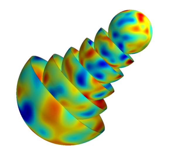
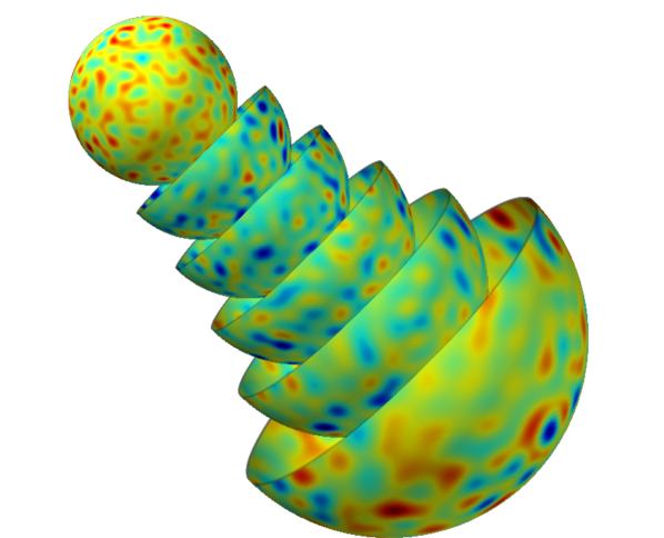
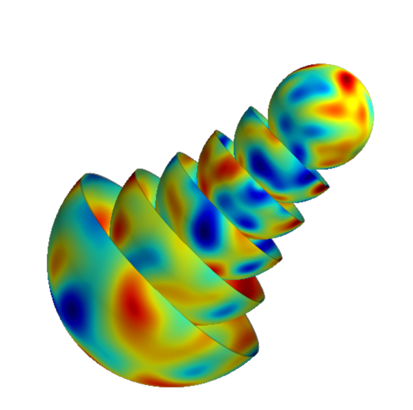
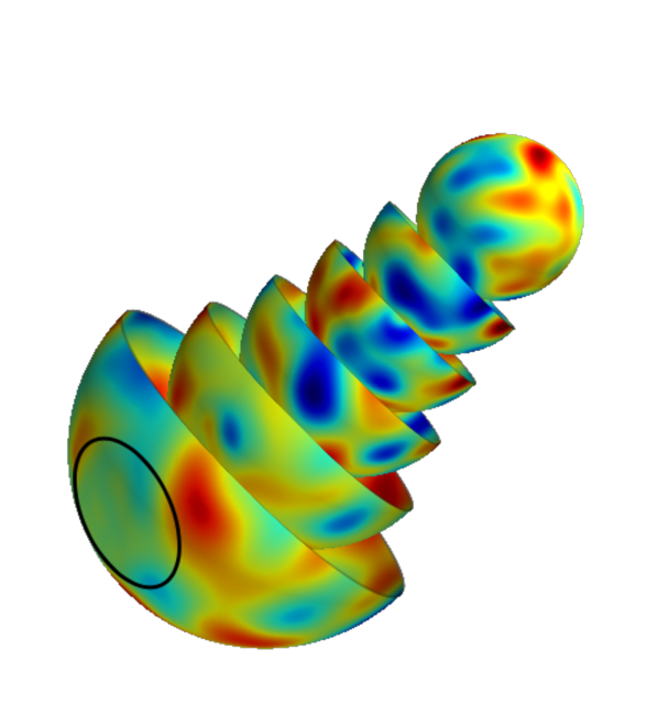
Figure 1: Description: Variational inference results for 3D directional deconvolution with inpainting using pseudo-Gaussian simulations for $L=P=32$ (upsampled to 128), roughly approximating physical fields e.g. atmospheric fields – these methods trivially extend to realistic simulations. Specifically the ground truth is smoothed with a directional kernel, 50% of observations are masked, and the remaining observations are corrupted with 30dB i.i.d. Gaussian noise $\bm{n}\sim\mathcal{N}(0,\sigma^{2})$. Panels: Input ground truth (top left), naive inversion (baseline, top right), maximum a posteriori (MAP) estimator using ball wavelet $\ell_{1}$ sparsity (bottom left), and Bayesian hypothesis test of local structure $\Omega$ (bottom right, see Section II-E). Discussion: Notice that naive direct inversion recovers a poor estimator (SNR = $-2.707$dB). Alternatively, treating the problem as a Bayesian variational problem not only recovers a very good estimate (SNR = $10.293$dB), but also supports principled uncertainty quantification. The Bayesian hypothesis test of local substructure $\Omega$ in the bottom right subfigure correctly determines the physicality of this feature at $99\%$-confidence. The MAP estimate and uncertainties were recovered in $\sim 2$ minutes of non-dedicated compute on a MacBook Air 2016 respectively, which can trivially sped up through e.g. OpenMP and MPI.

III Numerical experiment

In this section we consider a noisy inpainting directional deconvolution inverse problem, which is (seriously) ill-posed and ill-conditioned. Such an example is representative of a diverse set of practical applications. Consider again the problem setup outlined in Section II-D, where we model the acquisition of observations by the sensing operator

$$\bm{\mathsf{\Phi}}=\bm{\mathsf{M}}\bm{\mathsf{B}}^{-1}\bm{\mathsf{K}}\bm{\mathsf{B}}\quad\text{and}\quad\bm{\mathsf{\Phi}}^{\dagger}=\bm{\mathsf{B}}^{\dagger}\bm{\mathsf{K}}\bm{\mathsf{B}}^{-\dagger}\bm{\mathsf{M}}^{\dagger},$$ (13)

where $\bm{\mathsf{B}}$ and $\bm{\mathsf{B}}^{-1}$ represent forward and inverse spin-$0$ Spherical-Laguerre transforms (see Section II-A), $\bm{\mathsf{K}}$ is multiplication with a skewed Gaussian kernel in Spherical-Laguerre space (which is trivially self-adjoint), $\bm{\mathsf{M}}$ represents masking, and $\dagger$ denotes the operator adjoint. It is important to note that $\bm{\mathsf{B}}^{-1}\not=\bm{\mathsf{B}}^{\dagger}$ which is a poorly motivated approximation often adopted in settings involving spherical harmonic transforms. Additionally, we define as a baseline the naive direct inversion $\bm{x}^{\text{DIR}}=\bm{\mathsf{\Phi}}^{-1}\bm{y}$ for $\bm{\mathsf{\Phi}}^{-1}=\bm{\mathsf{B}}^{-1}\bm{\mathsf{K}}^{-1}\bm{\mathsf{B}}\bm{\mathsf{M}}^{\dagger}$, where $\bm{\mathsf{K}}^{-1}$ is simply division by the Spherical-Laguerre space convolutional kernel. As we are considering ill-posed inverse problems [36] the naive inverse $\bm{x}^{\text{DIR}}$ can give (potentially non-physical) solutions which lie far from the true signal. Moreover, the noise contribution, which is typically highly oscillatory, may (and often does) dominate the solution.

We consider the case in which $\bm{n}$ is independent and identically distributed noise drawn from a univariate Gaussian distribution $\bm{n}\sim\mathcal{N}(0,\sigma^{2})$. Our likelihood function is thus given by a Gaussian distribution with zero mean and variance $\sigma^{2}$. Suppose our prior knowledge indicates that $\bm{x}$ is likely to be sparsely distributed when projected into the ball wavelet dictionary $\bm{\mathsf{\Psi}}$, described in Section II-B. A prior distribution which naturally promotes sparsity is the Laplacian distribution, which one might adopt, such that the posterior is given by

$$P(\bm{x}|\bm{y};\bm{\mathsf{\Phi}})\propto\exp\bigg{(}\frac{-{}_{\mathbb{B}^{3}}\!\lVert\bm{\mathsf{\Phi}}\bm{x}-\bm{y}\rVert_{2}^{2}}{2\sigma^{2}}\bigg{)}\exp\big{(}-\lambda{}_{\Psi}\!\lVert\bm{\mathsf{\Psi}}^{\dagger}\bm{x}\rVert_{1}\big{)},$$ (14)

where ${}_{\mathbb{B}^{3}}\!\lVert\cdot\rVert$ and ${}_{\Psi}\!\lVert\cdot\rVert$ are the standard $\ell_{p}$-norms weighted by pixel-size so as to better approximate the continuous $\ell_{p}$-norms on the ball. By following the logic presented in Section II-D one finds the MAP estimate is given by

$$\bm{x}^{\text{MAP}}=\operatorname*{argmin}_{\bm{x}\in\mathbb{R}^{N_{\mathbb{B}^{3}}}}\bigg{\{}\frac{{}_{\mathbb{B}^{3}}\!\lVert\bm{\mathsf{\Phi}}\bm{x}-\bm{y}\rVert_{2}^{2}}{2\sigma^{2}}+\lambda{}_{\Psi}\!\lVert\bm{\mathsf{\Psi}}^{\dagger}\bm{x}\rVert_{1}\bigg{\}},$$ (15)

with regularization parameter $\lambda\in\mathbb{R}^{+}$ which we marginalize over [44], to maintain a principled Bayesian interpretation.

III-A Experiment details

We generate a ground truth signal $\bm{x}^{\text{TRUE}}$ by smoothing a random signal on the ball, effectively generating a pseudo-Gaussian random field, which is bandlimited at $L$ in the angular domain and $P=L$ along the radial line. This ground truth is mapped by $\bm{\mathsf{\Phi}}$ to simulated observations which are subsequently polluted with i.i.d. noise, drawn from a univariate Gaussian distribution, to form simulated observations $\bm{y}$, such that the input signal to noise ratio,

$$\text{SNR}=20\times\log_{10}\bigg{(}\frac{\lVert\bm{\mathsf{\Phi}}\bm{x}^{\text{TRUE}}\rVert_{2}}{\lVert\bm{\mathsf{\Phi}}\bm{x}^{\text{TRUE}}-\bm{y}\rVert_{2}}\bigg{)},$$ (16)

is 30dB. An analogous SNR definition is used to quantify the reconstruction fidelity between $\bm{x}$ and a recovered solution $\bm{x}^{*}$. Both the naive inversion (SNR$=-2.707$dB), and MAP (SNR$=10.293$dB) estimators are recovered, and are presented in Figure 1. Note that the variational solution is recovered in the analysis unconstrained setting through the proximal forward-backward algorithm [45, 37]. This dramatic improvement in reconstruction fidelity is compounded by the fact that our estimator also supports principled Bayesian uncertainty quantification, namely hypothesis testing of structure e.g. the diffuse, high intensity region $\Omega$ highlighted in Figure 1 was correctly determined to be physical at $99\%$ confidence.

IV Discussion & conclusions

Whilst there are many methods which consider reconstruction over the 3D ball by analyzing individual concatenated spherical shells, to the best of our knowledge, this is the first article which develops variational regularization methods natively on the ball. Leveraging recent developments in probability concentration theory, we demonstrate how MAP estimation (unconstrained optimization) permits principled uncertainty quantification. Our Bayesian variational approach benefits from the computational efficiency of convex optimization whilst facilitating principled uncertainty quantification. We demonstrate that our variational approach is effective at solving seriously ill-posed and ill-conditioned inverse problems on the ball, recovering very accurate, robust estimates of the underlying ground truth. In future collaborative work we will apply these methods to more realistic simulations and observational data, for a variety of application domains. As a bi-product of this work an open-source, flexible, scalable object oriented C++ software, B3INV was created which is constructed on the convex optimization package SOPT [46, 47, 48, 49]. Additionally, fast adjoint operators which were written and collected into the FLAG and FLAGLET codebases.

References

- [1] D. S. Tuch, “Q-ball imaging,” Magnetic Resonance in Medicine: An Official Journal of the International Society for Magnetic Resonance in Medicine, vol. 52, no. 6, pp. 1358–1372, 2004.
- [2] F. J. Simons et al., “Solving or resolving global tomographic models with spherical wavelets, and the scale and sparsity of seismic heterogeneity,” Geophysical Journal International, vol. 187, no. 2, pp. 969–988, Nov. 2011.
- [3] A. Marignier, A. M. G. Ferreira, and T. Kitching, “The probability of mantle plumes in global tomographic models,” Geochemistry, Geophysics, Geosystems, vol. 21, no. 9, p. e2020GC009276, 2020.
- [4] E. Kendall, A. Ferreira, S.-J. Chang, M. Witek, and D. Peter, “Constraints on the upper mantle structure beneath the pacific from 3-d anisotropic waveform modelling,” Journal of Geophysical Research: Solid Earth.
- [5] A. Heavens, “3D weak lensing,” MNRAS, vol. 343, no. 4, pp. 1327–1334, 08 2003.
- [6] B. Leistedt, J. D. McEwen, T. D. Kitching, and H. V. Peiris, “3D weak lensing with spin wavelets on the ball,” Physical Review D, vol. 92, no. 12, p. 123010, Dec. 2015.
- [7] W. Boomsma and J. Frellsen, “Spherical convolutions and their application in molecular modelling.” in Advances in Neural Information Processing Systems, vol. 2, 2017, p. 6.
- [8] J. D. McEwen, G. Puy, J. Thiran, P. Vandergheynst, D. Van De Ville, and Y. Wiaux, “Sparse image reconstruction on the sphere: Implications of a new sampling theorem,” IEEE Transactions on Image Processing, vol. 22, no. 6, pp. 2275–2285, 2013.
- [9] C. G. R. Wallis, Y. Wiaux, and J. D. McEwen, “Sparse Image Reconstruction on the Sphere: Analysis and Synthesis,” IEEE Transactions on Image Processing, vol. 26, pp. 5176–5187, Nov. 2017.
- [10] M. A. Price, L. Pratley, and J. D. McEwen, “Sparse image reconstruction on the sphere: a general approach with uncertainty quantification,” submitted to IEEE Transactions on Image Processing, p. arXiv:2105.04935, 5 2021.
- [11] D. L. Donoho, “Compressed sensing,” IEEE Transactions on information theory, vol. 52, no. 4, pp. 1289–1306, 2006.
- [12] E. J. Candès et al., “Compressive sampling,” 2006.
- [13] J. Y. H. Chan, B. Leistedt, T. D. Kitching, and J. D. McEwen, “Second-generation curvelets on the sphere,” IEEE Transactions on Signal Processing, vol. 65, no. 1, pp. 5–14, 2017.
- [14] Leistedt, B., McEwen, J. D., Vandergheynst, P., and Wiaux, Y., “S2let: A code to perform fast wavelet analysis on the sphere,” A&A, vol. 558, p. A128, 2013.
- [15] J. D. McEwen and M. A. Price, “Scale-discretised ridgelet transform on the sphere,” in 2019 27th European Signal Processing Conference (EUSIPCO), 2019, pp. 1–5.
- [16] V. Michel, “Wavelets on the 3 dimensional ball,” PAMM, vol. 5, no. 1, pp. 775–776, 2005.
- [17] M. Fengler, D. Michel, and V. Michel, ZAMM - Journal of Applied Mathematics and Mechanics, vol. 86, no. 11, pp. 856–873, 2006.
- [18] F. Lanusse, A. Rassat, and J. L. Starck, “Spherical 3D isotropic wavelets,” Journal of Astronomy & Astrophysics, vol. 540, p. A92, Apr. 2012.
- [19] C. Durastanti, Y. Fantaye, F. Hansen, D. Marinucci, and I. Z. Pesenson, “Simple proposal for radial 3d needlets,” Phys. Rev. D, vol. 90, p. 103532, Nov 2014.
- [20] Z. Khalid, R. A. Kennedy, and J. D. McEwen, “Slepian spatial-spectral concentration on the ball,” Applied and Computational Harmonic Analysis, vol. 40, no. 3, pp. 470–504, 2016.
- [21] B. Leistedt and J. D. McEwen, “Exact Wavelets on the Ball,” IEEE Transactions on Signal Processing, vol. 60, no. 12, pp. 6257–6269, Dec. 2012.
- [22] M. Pereyra, “Maximum-a-posteriori estimation with bayesian confidence regions,” SIAM Journal on Imaging Sciences, vol. 10, no. 1, pp. 285–302, 2017.
- [23] H. Pollard, “Representation of an analytic function by a laguerre series,” Annals of Mathematics, vol. 48, no. 2, pp. 358–365, 1947.
- [24] E. J. Weniger, “On the analyticity of Laguerre series,” Journal of Physics A Mathematical General, vol. 41, no. 42, p. 425207, Oct. 2008.
- [25] E. T. Newman and R. Penrose, “Note on the bondi-metzner-sachs group,” Journal of Mathematical Physics, vol. 7, no. 5, pp. 863–870, 1966.
- [26] J. N. Goldberg, A. J. Macfarlane, E. T. Newman, F. Rohrlich, and E. C. G. Sudarshan, “Spin-s spherical harmonics,” Journal of Mathematical Physics, vol. 8, no. 11, pp. 2155–2161, 1967.
- [27] J. D. McEwen and Y. Wiaux, “A Novel Sampling Theorem on the Sphere,” IEEE Transactions on Signal Processing, vol. 59, no. 12, pp. 5876–5887, Dec. 2011.
- [28] J. D. McEwen, B. Leistedt, M. Büttner, H. V. Peiris, and Y. Wiaux, “Directional spin wavelets on the sphere,” arXiv e-prints, p. arXiv:1509.06749, Sept. 2015.
- [29] X. Cai, M. Pereyra, and J. D. McEwen, “Uncertainty quantification for radio interferometric imaging: II. MAP estimation,” MNRAS, vol. 480, no. 3, pp. 4170–4182, Nov. 2018.
- [30] M. A. Price, X. Cai, J. D. McEwen, T. D. Kitching, and C. G. R. Wallis, “Sparse Bayesian mass-mapping with uncertainties: hypothesis testing of structure,” submitted to MNRAS, 2018.
- [31] M. A. Price, J. D. McEwen, L. Pratley, and T. D. Kitching, “Sparse Bayesian mass-mapping with uncertainties: Full sky observations on the celestial sphere,” MNRAS, vol. 500, no. 4, pp. 5436–5452, Jan. 2021.
- [32] W. H. Press, S. A. Teukolsky, W. T. Vetterling, and B. P. Flannery, Numerical Recipes 3rd Edition: The Art of Scientific Computing, 3rd ed. USA: Cambridge University Press, 2007.
- [33] J. D. McEwen and B. Leistedt, “Fourier-Laguerre transform, convolution and wavelets on the ball,” arXiv e-prints, p. arXiv:1307.1307, July 2013.
- [34] Y. Wiaux, J. D. McEwen, P. Vandergheynst, and O. Blanc, “Exact reconstruction with directional wavelets on the sphere,” MNRAS, vol. 388, no. 2, pp. 770–788, 07 2008.
- [35] J. D. McEwen, C. Durastanti, and Y. Wiaux, “Localisation of directional scale-discretised wavelets on the sphere,” Applied and Computational Harmonic Analysis, vol. 44, no. 1, pp. 59–88, 2018.
- [36] J. Hadamard, “Sur les problèmes aux dérivées partielles et leur signification physique,” Princeton university bulletin, pp. 49–52, 1902.
- [37] P. L. Combettes and J.-C. Pesquet, “Proximal splitting methods in signal processing,” in Fixed-point algorithms for inverse problems in science and engineering. Springer, 2011, pp. 185–212.
- [38] J. J. Moreau, “Fonctions convexes duales et points proximaux dans un espace hilbertien,” C.R. Acad. Sci. Paris Ser. A Math., vol. 255, pp. 2897–2899, 1962.
- [39] S. Boyd, N. Parikh, and E. Chu, Distributed optimization and statistical learning via the alternating direction method of multipliers. Now Publishers Inc, 2011.
- [40] M. A. Price, X. Cai, J. D. McEwen, M. Pereyra, and T. D. Kitching, “Sparse Bayesian mass mapping with uncertainties: local credible intervals,” MNRAS, vol. 492, no. 1, pp. 394–404, Dec. 2019.
- [41] M. Pereyra, “Proximal markov chain monte carlo algorithms,” Statistics and Computing, vol. 26, no. 4, pp. 745–760, 2016.
- [42] A. Repetti, M. Pereyra, and Y. Wiaux, “Scalable bayesian uncertainty quantification in imaging inverse problems via convex optimization,” SIAM Journal on Imaging Sciences, vol. 12, no. 1, pp. 87–118, 2019.
- [43] M. A. Price, J. D. McEwen, X. Cai, and T. D. Kitching, “Sparse Bayesian mass mapping with uncertainties: peak statistics and feature locations,” MNRAS, vol. 489, no. 3, pp. 3236–3250, 08 2019.
- [44] M. Pereyra, J. Bioucas-Dias, and M. Figueiredo, Maximum-a-posteriori estimation with unknown regularisation parameters, 12 2015, pp. 230–234.
- [45] A. Beck and M. Teboulle, “A fast iterative shrinkage-thresholding algorithm for linear inverse problems,” SIAM journal on imaging sciences, vol. 2, no. 1, pp. 183–202, 2009.
- [46] R. E. Carrillo, J. D. McEwen, and Y. Wiaux, “Sparsity Averaging Reweighted Analysis (SARA): a novel algorithm for radio-interferometric imaging,” MNRAS, vol. 426, no. 2, pp. 1223–1234, Oct. 2012.
- [47] R. E. Carrillo, J. D. McEwen, D. Van De Ville, J.-P. Thiran, and Y. Wiaux, “Sparsity Averaging for Compressive Imaging,” IEEE Signal Processing Letters, vol. 20, no. 6, pp. 591–594, June 2013.
- [48] A. Onose, R. E. Carrillo, A. Repetti, J. D. McEwen, J.-P. Thiran, J.-C. Pesquet, and Y. Wiaux, “Scalable splitting algorithms for big-data interferometric imaging in the SKA era,” MNRAS, vol. 462, no. 4, pp. 4314–4335, Nov. 2016.
- [49] L. Pratley, J. D. McEwen, M. d’Avezac, R. E. Carrillo, A. Onose, and Y. Wiaux, “Robust sparse image reconstruction of radio interferometric observations with PURIFY,” MNRAS, vol. 473, no. 1, pp. 1038–1058, Jan. 2018.