A monolithic fluid-porous structure interaction finite element method

Abstract

The paper introduces a fully discrete quasi-Lagrangian finite element method for a monolithic formulation of a fluid-porous structure interaction problem. The method is second order in time and allows a standard $P_{2}-P_{1}$ (Taylor–Hood) finite element spaces for fluid problems in both fluid and porous domains. The performance of the method is illustrated on a series of numerical experiments.

1 Introduction

Blood flow in a vessel with permeable walls or penetration of oil through a crack in a porous matrix can be seen as the interaction of a freely flowing fluid with a fluid-saturated poroelastic structure. A continuum mechanics description of such fluid-poroelastic phenomena often leads to coupled systems of (Navier–)Stokes and Biot equations [30, 22]. Recently, there has been a growing interest in the numerical solution of the Stokes–Biot and Navier–Stokes–Biot problems. Several authors suggested solution strategies based on decomposition of the system into fluid and poroelastic loosely coupled problems to allow for a computationally efficient time-stepping schemes [5, 8]. For the reason of better stability, monolithic methods for the (Navier–)Stokes–Biot equations have become popular in the literature. They differ in the form of equations and the numerical treatment of the coupling conditions on the interface between a free flow domain and a domain occupied by the porous structure. In [2] the continuity of fluid fluxes on the interface is imposed weakly with the help of a Lagrange multipier and in [31] an interior penalty discontinuous Galerkin method is applied to obtain a discrete coupled formulation. The Nitsche approach is used for coupling fluid and poroelastic finite element formulations in  [9, 1]. Combination of the Nitsche approach and unfitted finite elements [1] adds extra flexibility to the numerical solution.

Many publications on numerical methods for the fluid–poroelastic problem ignore inertia effect in the fluid and formulate the free fluid problem as a Stokes system. One reason for such simplification is the lack of the energy dissipation principle for the Navier–Stokes–Biot problem with the common interface conditions, which hinders the analysis in this case. This issue is well-known already for the Navier–Stokes–Darcy (the Navier–Stokes–Biot problem with rigid structure), where a local well-posedness of the system is currently known only under a smallness assumption (even in 2D) and the proof uses involved arguments that work in the absence of a priori energy bound [4, 19]. In the context of the Navier–Stokes–Darcy coupling the issue was addressed in [10, 11], where interface conditions were modified to ensure the thermodynamical consistency of the complete system. In this report, we follow [10, 11] and employ the suggested correction to the stress balance in the Navier–Stokes–Biot to end up with a dissipative system and stable numerical method.

We consider the Navier–Stokes–Biot system with the Beavers–Joseph–Saffman interface condition and a modified stress interface condition and discuss its energy balance. For an ALE formulation of the problem we further introduce a monolithic finite element method. Our finite element method features the formulation of all equations in the reference coordinates encoding all information on geometry deformation in solution-dependent coefficients. This formulation allows a simple application of the method of lines for the time discretization. In particular, the second order discretization in time is straightforward. Such monolithic approach was proved to be efficient for FSI problems with an impermeable elastic structure [20, 27, 28], and we extend it here to the case of poroelasticity. In the spirit of monolithic formulations we apply here the same finite elements to approximate fluid velocity and pressure in both domains. We choose the Taylor–Hood element (P2-P1) for this purpose, which is a valid Darcy element for applications where the local mass conservation is not critical [21]. We use the same P2 element for the structure velocity. To enforce the continuity of fluid flux through the interface, we use the penalty approach (the Nitsche approach as in [1] would be an alternative).

The remainder of the paper is organized in three sections. We formulate the governing equations, interface and boundary conditions in section 2. The same section presents the integral formulation, the energy balance of the system, and an ALE formulation that we use for the discretization. The finite element method is introduced in section 3. Section 4 presents results of several numerical experiments.

2 FPSI model

Consider a time-dependent domain $\Omega(t)\subset\mathbb{R}^{3}$ containing fluid and an elastic porous structure. A subdomain $\Omega^{f}(t)$ is entirely occupied by fluid and a subdomian $\Omega^{s}(t)$ is occupied by porous elastic solid fully saturated with fluid. These subdomains are non-overlapping and $\overline{\Omega(t)}=\overline{\Omega^{f}(t)}\cup\overline{\Omega^{s}(t)}$. Two regions are separated by the interface $\Gamma^{fs}(t):={\partial\Omega}^{f}(t)\cap{\partial\Omega}^{s}(t)$.

In this paper, the equations governing the fluid and solid motion will be written in the reference domains

$$\Omega_{f}=\Omega^{f}(0),\quad\Omega_{s}=\Omega^{s}(0),\quad\Gamma_{fs}=\Gamma^{fs}(0).$$

The deformation of the poroelastic part is given by the mapping

$$\mbox{\boldmath$\xi$\unboldmath}_{s}~{}:~{}\Omega_{s}\times[0,t]\to\bigcup_{t\in[0,T]}\Omega^{s}(t),$$

with the corresponding displacement $\mathbf{u}_{s}$, $\mathbf{u}_{s}(\mathbf{x},t):=\mathbf{x}-\mbox{\boldmath$\xi$\unboldmath}_{s}(\mathbf{x},t)$ and the velocity of the elastic structure $\mathbf{v}_{s}=\partial_{t}\mathbf{u}_{s}=-\partial_{t}\mbox{\boldmath$\xi$\unboldmath}_{s}(\mathbf{x},t)$.

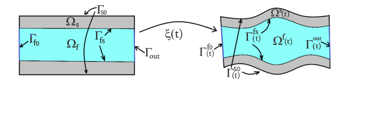
Figure 1: Reference and physical domains and boundaries.

The fluid dynamics is described by the velocity vector field $\mathbf{v}(\mathbf{x},t)$ and the pressure function $p(\mathbf{x},t)$ defined in the whole volume $\Omega(t)$ for all $t\in[0,T]$. Following [22, 5] we represent $\mathbf{v}$ in the poroelastic domain through the velocity of structure and the filtration flux $\mathbf{q}=\phi(\mathbf{v}-\mathbf{v}_{s})$, where $\phi$ is the known porosity coefficient. We denote the fluid pressure in the poroelastic domain by $p_{d}$, to emphasize its impact on the Darcy filtration, and in the fluid domain by $p_{f}$.

Denote by $\rho_{s}$ and $\rho_{f}$ the densities of solid and fluid. Then $\rho_{p}=\rho_{s}(1-\phi)+\rho_{f}\phi$ is the density of the saturated porous medium. Denote by $\mbox{\boldmath$\sigma$\unboldmath}_{s}$, $\mbox{\boldmath$\sigma$\unboldmath}_{f}$ the Cauchy stress tensors in porous media and fluid, respectively. The poroelastic stress tensor is given by $\mbox{\boldmath$\sigma$\unboldmath}_{p}=\mbox{\boldmath$\sigma$\unboldmath}_{s}-\alpha p\mathbf{I}$, where $\alpha>0$ is Biot’s coefficient (typically $\alpha\simeq 1$, so further we set $\alpha=1$). The porous medium is also characterized by its permeability tensor $K$. The Biot system in the porous domain and the Navier-Stokes equations in the fluid domain follow from the momenta balances and mass conservation principles (and neglecting the inertial effect of the matrix):

$$\begin{split}&\left\{\begin{split}\rho_{p}\dot{\mathbf{v}}_{s}+\rho_{f}\dot{\mathbf{q}}&={\rm div}\,\mbox{\boldmath$\sigma$\unboldmath}_{p}\\ \rho_{f}\dot{\mathbf{v}}_{s}+\frac{\rho_{f}}{\phi}\dot{\mathbf{q}}&=-(K^{-1}\mathbf{q}+\nabla p_{d})\\ -s_{0}\dot{p_{d}}&={\rm div}\,(\mathbf{v}_{s}+\mathbf{q})\end{split}\right.\quad\text{in}~{}\Omega^{s}(t),\\ &\left\{\begin{split}\rho_{f}\dot{\mathbf{v}}_{f}&={\rm div}\,\mbox{\boldmath$\sigma$\unboldmath}_{f}\\ {\rm div}\,\mathbb{v}_{f}&=0\end{split}\right.\quad\text{in}~{}\Omega^{f}(t),\end{split}$$ (1)

where $1/s_{0}$ is Biot modulus or mixture compressibility modulus.

We divide the boundary of $\Omega(t)$ into the external boundary of the poroplastic structure $\Gamma^{s0}(t):={\partial\Omega}(t)\cap{\partial\Omega}^{s}(t)$, fluid Dirichlet and outflow boundaries: ${\partial\Omega}(t)\cap{\partial\Omega}^{f}(t)=\Gamma^{f0}(t)\cup\Gamma^{\rm out}(t)$; cf. Figure 1. The governing equations are complemented with boundary conditions

$$\mathbb{v}^{f}=\mathbb{g}~{}\text{ on }\Gamma^{f0}(t),\quad\mbox{\boldmath$\sigma$\unboldmath}_{f}\mathbf{n}=\mathbb{0}\;\text{ on }\Gamma^{\rm out}(t),\quad p_{d}=0\;\text{ on }\Gamma^{s0}(t),\quad\mathbb{v}^{s}=\mathbb{0}~{}\text{ on }\Gamma^{s0}(t)$$ (2)

and suitable initial conditions.

We now discuss coupling conditions on the interface between the fluid and poroelastic domains. Denote by $\mathbf{n}$ the normal vector on $\Gamma^{fs}(t)$ pointing from the fluid to the poroelastic structure. The balance of normal stresses on $\Gamma^{fs}(t)$ is commonly written in terms of the interface conditions: $\mbox{\boldmath$\sigma$\unboldmath}_{f}\mathbf{n}=\mbox{\boldmath$\sigma$\unboldmath}_{p}\mathbf{n}$ and $\mathbf{n}^{T}\mbox{\boldmath$\sigma$\unboldmath}_{f}\mathbf{n}=-p_{d}$. This coupling, however, is not known to provide an energy consistent (dissipative) system. For the pure Darcy–Navier–Stokes coupling a remedy was suggested in [10, 12] where the second condition was changed to include a contribution of the fluid kinetic energy. In this paper, we use the same modification in the poroelasticity context and the two interface conditions read:

$$\mbox{\boldmath$\sigma$\unboldmath}_{f}\mathbf{n}=\mbox{\boldmath$\sigma$\unboldmath}_{p}\mathbf{n}\qquad\text{and}\quad\mathbf{n}^{T}\mbox{\boldmath$\sigma$\unboldmath}_{f}\mathbf{n}=-p_{d}+\frac{\rho_{f}}{2}|{\mathbf{v}}_{f}|^{2}~{}~{}~{}\text{on}~{}\Gamma^{fs}(t).$$ (3)

Such modification of the stress balance is similar to modifications of outflow boundary conditions and 1D-3D models coupling conditions in computational fluid dynamics, see e.g., [6, 7]. The continuity of the normal flux on the fluid-structure interface gives

$$\mathbf{v}_{f}\cdot\mathbf{n}=(\mathbf{v}_{s}+\mathbf{q})\cdot\mathbf{n}\quad\mbox{on}~{}\Gamma^{fs}(t).$$ (4)

Finally, the Beavers–Joseph–Saffman condition sets the tangential component of the normal stress proportional to the fluid “slip” rate along the interface:

$$\mathbf{P}\mbox{\boldmath$\sigma$\unboldmath}_{f}\mathbf{n}=-\gamma\mathbf{P}K^{-\frac{1}{2}}(\mathbf{v}_{f}-\mathbf{v}_{s})~{}~{}~{}\text{on}~{}\Gamma^{fs}(t),$$ (5)

where $\mathbf{P}$ is the orthogonal projector on the tangential plane to $\Gamma^{fs}(t)$.

2.1 Integral formulation

In the preparation for the finite element method, we write out an integral (weak) formulation of the FPSI problem (1)–(5). We take the inner product of the elasticity equation in (1) with a sufficiently smooth $\mbox{\boldmath$\psi$\unboldmath}_{s}$ such that $\mbox{\boldmath$\psi$\unboldmath}_{s}=0$ on $\Gamma^{s0}(t)$, integrate it over $\Omega^{s}(t)$ and integrate the stress term by parts (recall that $\mathbf{n}$ is inward for $\Omega^{s}$). This adds up with the first Darcy equation multiplied by a sufficiently smooth $\mbox{\boldmath$\psi$\unboldmath}_{d}$ and integrated over $\Omega^{s}(t)$ to give

$$\int_{\Omega^{s}(t)}(\rho_{p}\dot{\mathbf{v}}_{s}+\rho_{f}\dot{\mathbf{q}})\cdot\mbox{\boldmath$\psi$\unboldmath}_{s}+(\rho_{f}\dot{\mathbf{v}}_{s}+\frac{\rho_{f}}{\phi}\dot{\mathbf{q}}+K^{-1}\mathbf{q})\cdot\mbox{\boldmath$\psi$\unboldmath}_{d}\,dx+\int_{\Omega^{s}(t)}\mbox{\boldmath$\sigma$\unboldmath}_{p}:\nabla\mbox{\boldmath$\psi$\unboldmath}_{s}\,dx\\ -\int_{\Omega^{s}(t)}p_{d}{\rm div}\,\mbox{\boldmath$\psi$\unboldmath}_{d}+\int_{\Gamma^{fs}(t)}(\mbox{\boldmath$\sigma$\unboldmath}_{p}\mathbf{n})\cdot\mbox{\boldmath$\psi$\unboldmath}_{s}\,ds-\int_{\Gamma^{fs}(t)}p_{d}(\mbox{\boldmath$\psi$\unboldmath}_{d}\cdot\mathbf{n})\,ds=0.$$ (6)

Further, the fluid momentum equation in (1) is multiplied by a smooth vector function $\mbox{\boldmath$\psi$\unboldmath}_{f}$ such that $\mbox{\boldmath$\psi$\unboldmath}_{f}=\mathbb{0}$ on $\Gamma^{f0}$. Integrating over $\Omega^{s}(t)$ and integrating the stress term by parts we obtain

$$\int_{\Omega^{f}(t)}\rho_{f}\dot{\mathbf{v}}_{f}\cdot\mbox{\boldmath$\psi$\unboldmath}_{f}\,dx+\int_{\Omega^{f}(t)}\mbox{\boldmath$\sigma$\unboldmath}_{f}:\nabla\mbox{\boldmath$\psi$\unboldmath}_{f}\,dx-\int_{\Gamma^{fs}(t)}\mbox{\boldmath$\psi$\unboldmath}_{f}^{T}\mbox{\boldmath$\sigma$\unboldmath}_{f}\mathbf{n}\,ds=0.$$ (7)

We add up boundary terms in (6) and (7) and use interface conditions (3)–(5) to reorganize them

$$\int_{\Gamma^{fs}(t)}(\mbox{\boldmath$\sigma$\unboldmath}_{p}\mathbf{n})\cdot \mbox{\boldmath$\psi$\unboldmath}_{s}\,ds-\int_{\Gamma^{fs}(t)}p_{d}(\mbox{\boldmath$\psi$\unboldmath}_{d}\cdot\mathbf{n})\,ds-\int_{\Gamma^{fs}(t)}\mbox{\boldmath$\psi$\unboldmath}_{f}^{T}\mbox{\boldmath$\sigma$\unboldmath}_{f}\mathbf{n}\,ds$$

use (3) $$=\int_{\Gamma^{fs}(t)}(\mbox{\boldmath$\sigma$\unboldmath}_{f}\mathbf{n})\cdot(\mbox{\boldmath$\psi$\unboldmath}_{s}-\mbox{\boldmath$\psi$\unboldmath}_{f})\,ds-\int_{\Gamma^{fs}(t)}p_{d}(\mbox{\boldmath$\psi$\unboldmath}_{d}\cdot\mathbf{n})\,ds$$

$$\text{\footnotesize split }\mbox{\boldmath$\sigma$\unboldmath}_{f}\mathbf{n} =\int_{\Gamma^{fs}(t)}(\mathbf{n}^{T}\mbox{\boldmath$\sigma$\unboldmath}_{f}\mathbf{n})(\mbox{\boldmath$\psi$\unboldmath}_{s}-\mbox{\boldmath$\psi$\unboldmath}_{f})\cdot\mathbf{n}\,ds+\int_{\Gamma^{fs}(t)}(\mathbf{P}\mbox{\boldmath$\sigma$\unboldmath}_{f}\mathbf{n})\cdot\mathbf{P}(\mbox{\boldmath$\psi$\unboldmath}_{s}-\mbox{\boldmath$\psi$\unboldmath}_{f})\,ds$$

$$-\int_{\Gamma^{fs}(t)}p_{d}(\mbox{\boldmath$\psi$\unboldmath}_{d}\cdot\mathbf{n})\,ds$$

use (3), (5) $$=\int_{\Gamma^{fs}(t)}p_{d}(\mbox{\boldmath$\psi$\unboldmath}_{f}-\mbox{\boldmath$\psi$\unboldmath}_{s}-\mbox{\boldmath$\psi$\unboldmath}_{d})\cdot\mathbf{n}\,ds+\gamma\int_{\Gamma^{fs}(t)}K^{-\frac{1}{2}}\mathbf{P}(\mathbf{v}_{f}-\mathbf{v}_{s})\cdot(\mbox{\boldmath$\psi$\unboldmath}_{f}-\mbox{\boldmath$\psi$\unboldmath}_{s})\,ds$$

$$\qquad+\int_{\Gamma^{fs}(t)}\frac{\rho_{f}}{2}|{\mathbf{v}}_{f}|^{2}(\mbox{\boldmath$\psi$\unboldmath}_{s}-\mbox{\boldmath$\psi$\unboldmath}_{f})\cdot\mathbf{n}\,ds.$$

Summing up (6) and (7) and using the calculations above we arrive at the integral equality satisfied by sufficiently smooth FPSI solution $\mathbf{v}_{s}$, $\mathbf{q}$, $\mathbf{v}_{f}$, $p_{d}$, $p_{f}$

$$\int_{\Omega^{s}(t)}\left[(\rho_{p}\dot{\mathbf{v}}_{s}+\rho_{f}\dot{\mathbf{q}})\cdot\mbox{\boldmath$\psi$\unboldmath}_{s}+(\rho_{f}\dot{\mathbf{v}}_{s}+\frac{\rho_{f}}{\phi}\dot{\mathbf{q}}+K^{-1}\mathbf{q})\cdot\mbox{\boldmath$\psi$\unboldmath}_{d}\right]\,dx+\int_{\Omega^{s}(t)}\mbox{\boldmath$\sigma$\unboldmath}_{p}:\nabla\mbox{\boldmath$\psi$\unboldmath}_{s}\,dx\\ -\int_{\Omega^{s}(t)}p_{d}{\rm div}\,\mbox{\boldmath$\psi$\unboldmath}_{d}\,dx+\int_{\Omega^{f}(t)}\rho_{f}\dot{\mathbf{v}}_{f}\cdot\mbox{\boldmath$\psi$\unboldmath}_{f}\,dx+\int_{\Omega^{f}(t)}\mbox{\boldmath$\sigma$\unboldmath}_{f}:\nabla\mbox{\boldmath$\psi$\unboldmath}_{f}\,dx+\int_{\Gamma^{fs}(t)}\frac{\rho_{f}}{2}|{\mathbf{v}}_{f}|^{2}(\mbox{\boldmath$\psi$\unboldmath}_{s}-\mbox{\boldmath$\psi$\unboldmath}_{f})\cdot\mathbf{n}\,ds\\ +\int_{\Gamma^{fs}(t)}p_{d}(\mbox{\boldmath$\psi$\unboldmath}_{f}-\mbox{\boldmath$\psi$\unboldmath}_{s}-\mbox{\boldmath$\psi$\unboldmath}_{d})\cdot\mathbf{n}\,ds+\gamma\int_{\Gamma^{fs}(t)}K^{-\frac{1}{2}}\mathbf{P}(\mathbf{v}_{f}-\mathbf{v}_{s})\cdot(\mbox{\boldmath$\psi$\unboldmath}_{f}-\mbox{\boldmath$\psi$\unboldmath}_{s})\,ds=0$$ (8)

for all sufficiently smooth $\mbox{\boldmath$\psi$\unboldmath}_{s}$, $\mbox{\boldmath$\psi$\unboldmath}_{d}$, and $\mbox{\boldmath$\psi$\unboldmath}_{f}$ such that $\mbox{\boldmath$\psi$\unboldmath}_{s}=0$ on $\Gamma^{s0}$, $\mbox{\boldmath$\psi$\unboldmath}_{f}=\mathbb{0}$ on $\Gamma^{f0}$. For the weak formulation, this integral identity should be supplemented by the two continuity equations in (1) and the normal continuity interface condition (4).

To obtain the energy balance identity, we assume that $\Gamma^{f0}$ and $\Gamma^{\rm out}$ are steady and $\mathbf{g}=0$ on $\Gamma^{f0}$. We further let $\mbox{\boldmath$\psi$\unboldmath}_{s}=\mathbf{v}_{s}$, $\mbox{\boldmath$\psi$\unboldmath}_{d}=\mathbf{q}$, $\mbox{\boldmath$\psi$\unboldmath}_{f}=\mathbf{v}_{f}$ and use $\mbox{\boldmath$\sigma$\unboldmath}_{p}=\mbox{\boldmath$\sigma$\unboldmath}_{s}-p\mathbf{I}$, continuity conditions and (4) to arrive at the equality:

$$\int_{\Omega^{s}(t)}\left[(\rho_{p}\dot{\mathbf{v}}_{s}+\rho_{f}\dot{\mathbf{q}})\cdot\mathbf{v}_{s}+(\rho_{f}\dot{\mathbf{v}}_{s}+\frac{\rho_{f}}{\phi}\dot{\mathbf{q}})\cdot\mathbf{q}+K^{-1}|\mathbf{q}|^{2}\right]\,dx+\int_{\Omega^{s}(t)}\mbox{\boldmath$\sigma$\unboldmath}_{s}:\nabla\mbox{\boldmath$\psi$\unboldmath}_{s}\,dx+\int_{\Omega^{s}(t)}s_{0}\dot{p}_{d}p_{d}\,dx\\ +\int_{\Omega^{f}(t)}\rho_{f}\dot{\mathbf{v}}_{f}\cdot\mathbf{v}_{f}\,dx+\int_{\Omega^{f}(t)}\mbox{\boldmath$\sigma$\unboldmath}_{f}:\nabla\mathbf{v}_{f}\,dx-\int_{\Gamma^{fs}(t)}\frac{\rho_{f}}{2}|{\mathbf{v}}_{f}|^{2}\mathbf{q}\cdot\mathbf{n}\,ds+\gamma\int_{\Gamma^{fs}(t)}K^{-\frac{1}{2}}|\mathbf{P}(\mathbf{v}_{f}-\mathbf{v}_{s})|^{2}\,ds=0.$$ (9)

Using $\mbox{\boldmath$\sigma$\unboldmath}_{f}=\mu_{f}\mathbf{D}\mathbf{v}_{f}-p_{f}\mathbf{I}$, ${\rm div}\,\mathbf{v}_{f}=0$, and rearranging the first two term by substituting $\rho_{p}=\rho_{s}(1-\phi)+\rho_{f}\phi$, we can rewrite the above equality as

$$\int_{\Omega^{s}(t)}\left[(1-\phi)\rho_{s}\dot{\mathbf{v}}_{s}\cdot\mathbf{v}_{s}+\phi\rho_{f}(\dot{\mathbf{v}}_{s}+\frac{\dot{\mathbf{q}}}{\phi})\cdot({\mathbf{v}}_{s}+\frac{\mathbf{q}}{\phi})\right]\,dx+\int_{\Omega^{s}(t)}K^{-1}|\mathbf{q}|^{2}\,dx+\int_{\Omega^{s}(t)}\mbox{\boldmath$\sigma$\unboldmath}_{s}:\nabla\mbox{\boldmath$\psi$\unboldmath}_{s}\,dx\\ +\int_{\Omega^{s}(t)}s_{0}\dot{p}_{d}p_{d}\,dx+\int_{\Omega^{f}(t)}\rho_{f}\dot{\mathbf{v}}_{f}\cdot\mathbf{v}_{f}\,dx+\mu_{f}\int_{\Omega^{f}(t)}|\mathbf{D}\mathbf{v}_{f}|^{2}\,dx\\ -\int_{\Gamma^{fs}(t)}\frac{\rho_{f}}{2}|{\mathbf{v}}_{f}|^{2}\mathbf{q}\cdot\mathbf{n}\,ds+\gamma\int_{\Gamma^{fs}(t)}K^{-\frac{1}{2}}|\mathbf{P}(\mathbf{v}_{f}-\mathbf{v}_{s})|^{2}\,ds=0.$$ (10)

The integrals with material derivatives can be readily converted to the variations of kinetic energy by application of the Reynolds transport theorem and recalling that all parts of $\partial\Omega^{f}(t)$ are steady except $\Gamma^{fs}(t)$, which normal velocity is $\mathbf{v}_{s}\cdot\mathbf{n}$:

$$\begin{split}\frac{d}{dt}\frac{1}{2}\int_{\Omega^{f}(t)}\rho_{f}|{\mathbf{v}}_{f}|^{2}\,dx&=\int_{\Gamma^{fs}(t)}\rho_{f}\frac{\partial{\mathbf{v}}_{f}}{\partial t}\cdot{\mathbf{v}}_{f}\,ds+\frac{1}{2}\int_{\Gamma^{fs}(t)}\rho_{f}|{\mathbf{v}}_{f}|^{2}\mathbf{v}_{s}\cdot\mathbf{n}\,ds\\ &=\int_{\Gamma^{fs}(t)}\rho_{f}\frac{\partial{\mathbf{v}}_{f}}{\partial t}\cdot{\mathbf{v}}_{f}\,ds+\frac{1}{2}\int_{\Gamma^{fs}(t)}\rho_{f}|{\mathbf{v}}_{f}|^{2}\mathbf{v}_{f}\cdot\mathbf{n}\,ds-\frac{1}{2}\int_{\Gamma^{fs}(t)}\rho_{f}|{\mathbf{v}}_{f}|^{2}\mathbf{q}\cdot\mathbf{n}\,ds\\ &=\int_{\Gamma^{fs}(t)}\rho_{f}\frac{\partial{\mathbf{v}}_{f}}{\partial t}\cdot{\mathbf{v}}_{f}\,ds+\frac{1}{2}\int_{\Gamma^{fs}(t)}\rho_{f}{\rm div}\,(|{\mathbf{v}}_{f}|^{2}{\mathbf{v}}_{f})\,ds-\frac{1}{2}\int_{\Gamma^{fs}(t)}\rho_{f}|{\mathbf{v}}_{f}|^{2}\mathbf{q}\cdot\mathbf{n}\,ds\\ \text{\footnotesize using }{\footnotesize{\rm div}\,{\mathbf{v}}_{f}=0}~{}&=\int_{\Gamma^{fs}(t)}\rho_{f}\frac{\partial{\mathbf{v}}_{f}}{\partial t}\cdot{\mathbf{v}}_{f}\,ds+\int_{\Gamma^{fs}(t)}\rho_{f}((\mathbf{v}_{f}\cdot\nabla){\mathbf{v}}_{f})\cdot{\mathbf{v}}_{f}\,ds-\frac{1}{2}\int_{\Gamma^{fs}(t)}\rho_{f}|{\mathbf{v}}_{f}|^{2}\mathbf{q}\cdot\mathbf{n}\,ds\\ &=\int_{\Gamma^{fs}(t)}\rho_{f}\dot{\mathbf{v}}_{f}\cdot{\mathbf{v}}_{f}\,ds-\frac{1}{2}\int_{\Gamma^{fs}(t)}\rho_{f}|{\mathbf{v}}_{f}|^{2}\mathbf{q}\cdot\mathbf{n}\,ds.\end{split}$$

We handle the $\int_{\Omega^{s}(t)}$ integrals containing material derivatives in (10) by the same argument assuming that the elastic structure is incompressible, i.e. ${\rm div}\,\mathbf{v}_{s}=0$, and recalling that the material derivative in the structure is written in the Eulerian terms as $\partial/{\partial t}+\mathbf{v}_{s}\cdot\nabla$. Therefore, (10) yields

$$\frac{d}{dt}\frac{1}{2}\int_{\Omega^{s}(t)}(1-\phi)\rho_{s}|\mathbf{v}_{s}|^{2}+\phi\rho_{f}|\mathbf{v}_{f}|^{2}\,dx+\int_{\Omega^{s}(t)}K^{-1}|\mathbf{q}|^{2}\,dx+\int_{\Omega^{s}(t)}\mbox{\boldmath$\sigma$\unboldmath}_{s}:\nabla\mbox{\boldmath$\psi$\unboldmath}_{s}\,dx\\ +\frac{d}{dt}\frac{1}{2}\int_{\Omega^{s}(t)}s_{0}|{p}_{d}|^{2}\,dx+\frac{d}{dt}\frac{1}{2}\int_{\Omega^{f}(t)}\rho_{f}|{\mathbf{v}}_{f}|^{2}\,dx+\mu_{f}\int_{\Omega^{f}(t)}|\mathbf{D}\mathbf{v}_{f}|^{2}\,dx\\ +\gamma\int_{\Gamma^{fs}(t)}K^{-\frac{1}{2}}|\mathbf{P}(\mathbf{v}_{f}-\mathbf{v}_{s})|^{2}\,ds=0,$$ (11)

where we used $\mathbf{v}_{f}=\mathbf{v}_{s}+\frac{\mathbf{q}}{\phi}$ in $\Omega^{s}(t)$ for the brevity. We see that the system is dissipative. Without the correction in the stress balance on the interface, the sign indefinite term $-\frac{\rho_{f}}{2}\int_{\Gamma^{fs}(t)}|{\mathbf{v}}_{f}|^{2}(\mathbf{q}\cdot\mathbf{n})\,ds$ appears in the energy equality, and the system is not necessarily dissipative.

2.2 ALE formulation

In this paper, we adopt the Arbitrary Lagrangian-Eulerian formulation by extending $\mbox{\boldmath$\xi$\unboldmath}_{s}$ to an auxiliary mapping in the fluid domain

$$\mbox{\boldmath$\xi$\unboldmath}_{f}~{}:~{}\Omega_{f}\times[0,t]\to\bigcup_{t\in[0,T]}\Omega^{f}(t)$$

such that $\mbox{\boldmath$\xi$\unboldmath}_{s}=\mbox{\boldmath$\xi$\unboldmath}_{f}$ on $\Gamma_{fs}$, i.e. $\xi$ is globally continuous. In general, $\mbox{\boldmath$\xi$\unboldmath}_{f}$ does not follow material trajectories. Instead, it is defined by a continuous extension of the displacement field to the flow reference domain

$$\mathbf{u}_{f}:=\mbox{Ext}(\mathbf{u}_{s})=\mathbf{x}-\mbox{\boldmath$\xi$\unboldmath}_{f}(\mathbf{x},t)\quad\mbox{in}~{}\Omega_{f}\times[0,t];\quad\mathbf{u}=\left\{\begin{split}\mathbf{u}_{s}&\text{ in }\Omega_{s}\\ \mathbf{u}_{f}&\text{ in }\Omega_{f}.\end{split}\right.$$ (12)

The corresponding globally defined deformation gradient is $\mathbf{F}=\mathbf{I}+\nabla\mathbf{u}$, and $J:=\mbox{det}(\mathbf{F})$ is its determinant. From now on, for notational simplicity, we will be using the same notation for these fields defined in the reference configuration as $\mathbf{v}_{f}(\mathbf{x},t):=\mathbf{v}_{f}(\mbox{\boldmath$\xi$\unboldmath}_{f}(\mathbf{x},t),t)$ and $p_{f}(\mathbf{x},t):=p_{f}(\mbox{\boldmath$\xi$\unboldmath}_{f}(\mathbf{x},t),t)$. We use the notation $\mbox{\boldmath$\sigma$\unboldmath}_{s}\circ\mbox{\boldmath$\xi$\unboldmath}_{s}(\mathbf{x}):=\mbox{\boldmath$\sigma$\unboldmath}_{s}(\mbox{\boldmath$\xi$\unboldmath}_{s}(\mathbf{x}))$.

The governing equations driving the motion of fluid and structure written in the reference domains read as

$$\left\{\begin{split}\rho_{p}\frac{\partial\mathbb{v}_{s}}{\partial t}+\rho_{f}\frac{\partial\mathbb{q}}{\partial t}=J^{-1}{\rm div}\,(J(\mbox{\boldmath$\sigma$\unboldmath}_{p}\circ\mbox{\boldmath$\xi$\unboldmath}_{s})\mathbf{F}^{-T})\quad\text{in}~{}\Omega_{s},\\ \rho_{f}\frac{\partial\mathbb{v}_{s}}{\partial t}+\frac{\rho_{f}}{\phi}\frac{\partial\mathbb{q}}{\partial t}=-K^{-1}\mathbf{q}-\mathbf{F}^{-T}\nabla p\quad\text{in}~{}\Omega_{s},\\ \rho_{f}\frac{\partial\mathbb{v}_{f}}{\partial t}=J^{-1}{\rm div}\,(J(\mbox{\boldmath$\sigma$\unboldmath}_{f}\circ\mbox{\boldmath$\xi$\unboldmath}_{f})\mathbf{F}^{-T})-\rho_{f}\nabla\mathbb{v}_{f}(\mathbf{F}^{-1}(\mathbb{v}_{f}-\frac{\partial\mathbb{u}}{\partial t}))\quad\text{in}~{}\Omega_{f},\end{split}\right.$$ (13)

and the mass conservation reads as

$$\left\{\begin{split}{\rm div}\,(J\mathbf{F}^{-1}(\mathbb{v}_{s}+\mathbf{q}))=-s_{0}J\frac{\partial p_{d}}{\partial t}&~{}~{}~{}\text{in}~{}\Omega_{s},\\ {\rm div}\,(J\mathbf{F}^{-1}\mathbb{v}_{f})=0&~{}~{}~{}\text{in}~{}\Omega_{f}.\end{split}\right.$$ (14)

Using the identity ${\rm div}\,(J\mathbf{F}^{-1}\mathbb{v})=J\nabla\mathbf{v}:\mathbf{F}^{-T}$, the last two equations can be written as

$$\left\{\begin{split}\nabla(\mathbb{v}_{s}+\mathbf{q}):\mathbf{F}^{-T}=-s_{0}\frac{\partial p_{d}}{\partial t}&~{}~{}~{}\text{in}~{}\Omega_{s},\\ \nabla\mathbf{v}_{f}:\mathbf{F}^{-T}=0&~{}~{}~{}\text{in}~{}\Omega_{f}.\end{split}\right.$$ (15)

The deformation of the structure can be found by integrating the kinematic equation

$$\frac{\partial\mathbb{u}_{s}}{\partial t}=\mathbf{v}_{s}~{}~{}~{}\text{in}~{}\Omega_{s}.$$ (16)

The boundary and interface conditions are the same in the ALE formulation. The normal $\mathbf{n}$ (and projector $\mathbf{P}=\mathbf{I}-\mathbf{n}\mathbf{n}^{T}$) to the interface and outflow boundary in the physical domain can be computed from the reference normal $\widehat{\mathbf{n}}$, i.e. $\mathbf{n}=\mathbf{F}^{-T}\widehat{\mathbf{n}}/|\mathbf{F}^{-T}\widehat{\mathbf{n}}|$. We collect all conditions in one place here:

$$\mathbb{v}_{f}=\mathbb{g}~{}\text{ on }\Gamma_{f0},\quad\mbox{\boldmath$\sigma$\unboldmath}_{f}\widehat{\mathbf{n}}=\mathbb{0}\;\text{ on }\Gamma_{\rm out},\quad\mathbb{v}_{s}=\mathbb{0}~{}\text{ on }\Gamma_{s0},\quad p_{d}=0~{}\text{ on }\Gamma_{s0}$$ (17)

for the outer boundaries and

$$\mbox{\boldmath$\sigma$\unboldmath}_{f}\mathbf{n}=\mbox{\boldmath$\sigma$\unboldmath}_{p}\mathbf{n},\qquad\mathbf{n}^{T}\mbox{\boldmath$\sigma$\unboldmath}_{f}\mathbf{n}=-p_{d}+\frac{\rho_{f}}{2}|{\mathbf{v}}_{f}|^{2}~{}~{}~{}\text{on}~{}\Gamma_{fs},$$ (18)

$$\mathbf{v}_{f}\cdot\mathbf{n}=(\mathbf{v}_{s}+\mathbf{q})\cdot\mathbf{n}\quad\mbox{on}~{}\Gamma_{fs},$$ (19)

$$\mathbf{P}\mbox{\boldmath$\sigma$\unboldmath}_{f}\mathbf{n}=-\gamma\mathbf{P}K^{-\frac{1}{2}}(\mathbf{v}_{f}-\mathbf{v}_{s})~{}~{}~{}\text{on}~{}\Gamma_{fs}$$ (20)

on the interface. For the integral formulation in the reference coordinates, we will use the identities $J\,d\hat{x}=dx$, $J|\mathbf{F}^{-T}\widehat{\mathbf{n}}|\,\,d\hat{s}=ds$, where $ds$, $d\hat{s}$ are elementary areas orthogonal to $\mathbf{n}$ and $\widehat{\mathbf{n}}$ in physical and reference coordinates, respectively.

The constitutive relation for the Newtonian fluid in the reference domain reads

$$\mbox{\boldmath$\sigma$\unboldmath}_{f}=-p_{f}\mathbf{I}+\mu_{f}(\nabla\mathbf{v}\mathbf{F}^{-1}+\mathbf{F}^{-T}(\nabla\mathbf{v})^{T})~{}~{}~{}\text{in}~{}\Omega_{f}.$$ (21)

For the structure we consider the compressible geometrically nonlinear Saint Venant–Kirchhoff material with

$$\mbox{\boldmath$\sigma$\unboldmath}_{s}=\frac{1}{J}\mathbf{F}\mathbf{S}\mathbf{F}^{T},\quad\text{with}~{}\mathbf{S}=\lambda_{s}\mbox{tr}(\mathbf{E}){\mathbf{I}}+2\mu_{s}\mathbf{E},$$ (22)

where $\mathbf{E}=\frac{1}{2}\left(\mathbf{F}^{T}\mathbf{F}-\mathbf{I}\right)$ is the Lagrange-Green strain tensor and $\lambda_{s},\mu_{s}$ are the Lame constants.

Thus, the FPSI problem in the reference coordinates consists in finding pressure distributions $p_{d}$, $p_{f}$, fluid and structure velocity fields $\mathbf{v}_{f}$, $\mathbf{v}_{s}$, fluid flux in the porous medium $\mathbf{q}$ and the displacement field $\mathbf{u}$ satisfying the set of equations, interface and boundary conditions (13)–(20), together with (21), (22), and subject to a given extension rule (12).

3 Discretization

We now proceed with dicretization of the FPSI problem formulated in the reference domain. Treating the problem in the reference domain allows us to avoid time-dependent triangulations and finite element function spaces and apply the standard method of lines to decouple space and time discretizations. We adopt a finite element method in space and define an admissible triangulation of the reference domain $\overline{\Omega}(0)$ as a collection ${\cal T}_{h}$ of shape-regular tetrahedra such that the triangulation respects the interface $\Gamma_{fs}$. This implies that ${\cal T}_{h}^{a}:=\{T\in{\cal T}_{h}\,:\,T\subset\Omega_{a}\}$, $a\in\{f,s\}$, are admissible triangulations of the fluid and poroelastic reference domains $\Omega_{a}$, $a\in\{f,s\}$. We exploit the finite element Taylor–Hood spaces which are popular in incompressible hydrodynamics:

$$\begin{split}\mathbb{V}_{h}^{a}&=\{\mathbf{v}\in C(\Omega_{a})\,:\,\mathbf{v}|_{T}\in P_{2}(T)^{3}\quad\forall\,T\in{\cal T}_{h}^{a}\},\quad a\in\{f,s\},\\ \mathbb{Q}_{h}^{a}&=\{q\in C(\Omega_{a})\,:\,q|_{T}\in P_{1}(T)\quad\forall\,T\in{\cal T}_{h}^{a}\},\quad a\in\{f,s\}.\end{split}$$

For trial functions we need also the following subspaces:

$$\begin{split}\mathbb{V}_{h}^{a,0}&=\{\mathbf{v}\in\mathbb{V}_{h}^{a}\,:\,\mathbf{v}|_{\Gamma_{a,0}}=\mathbf{0}\},\quad a\in\{f,s\},\\ \mathbb{Q}_{h}^{s,0}&=\{q\in\mathbb{Q}_{h}^{s}\,:\,q|_{\Gamma_{s,0}}={0}\}.\\ \end{split}$$

We note that the Taylor–Hood is not a standard Darcy element for $H(div)$- formulations of the problem. In particular, it fails to provide elementwise mass conservation. However, for applications where the local mass conservation is not a major concern, it is a legitimate choice leading to optimal convergence in the Darcy region in product $L^{2}$-velocity–$H^{1}$-pressure norm [21].

For the time discretization, we assume a constant time step $\Delta t$ and use the notation $f^{k}(\mathbf{x})\approx f(k\Delta t,\mathbf{x})$ for all time-dependent quantities. The first or second order backward finite difference approximation $\left[\frac{\partial f}{\partial t}\right]^{k}$ of the time derivative of $f$ at $t=k\Delta t$ is

$$\left[\frac{\partial f}{\partial t}\right]^{k}=\frac{f^{k}-f^{k-1}}{\Delta t}\quad\text{or}\quad\left[\frac{\partial f}{\partial t}\right]^{k}=\frac{3f^{k}-4f^{k-1}+f^{k-2}}{2\Delta t},$$

respectively. By $\widetilde{f}^{k}$ we denote the extrapolated quantity $f$

$$\widetilde{f}^{k}:=f^{k-1}\quad\text{or}\quad\widetilde{f}^{k}:=2f^{k-1}-f^{k-2}$$

for the first or second order extrapolation, respectively.

We proceed to multi-linear forms needed for our finite element formulation. For time derivatives, we need the form:

$$m^{k}(\mathbf{w}_{s},\mathbf{w}_{d},\mathbf{w}_{f},r;\mbox{\boldmath$\psi$\unboldmath}_{s},\mbox{\boldmath$\psi$\unboldmath}_{d},\mbox{\boldmath$\psi$\unboldmath}_{f},q):=\int_{\Omega_{s}}\tilde{J}^{k}(\rho_{p}\mathbf{w}_{s}+\rho_{f}\mathbf{w}_{d})\mbox{\boldmath$\psi$\unboldmath}_{s}\,\mathrm{d}x\\ +\int_{\Omega_{s}}\tilde{J}^{k}(\rho_{f}\mathbf{w}_{s}+\frac{\rho_{f}}{\phi}\mathbf{w}_{d})\mbox{\boldmath$\psi$\unboldmath}_{d}\,\mathrm{d}x+\int_{\Omega_{s}}s_{0}\tilde{J}^{k}r\,q\,\mathrm{d}x+\int_{\Omega_{f}}\rho_{f}\tilde{J}^{k}\mathbf{w}_{f}\mbox{\boldmath$\psi$\unboldmath}_{f}\,\mathrm{d}x.$$

For the elasticity part, we define

$$a_{s}^{k}(\mathbf{w}_{s},\mbox{\boldmath$\psi$\unboldmath}_{s})=\int_{\Omega_{s}}\mathbf{F}({\tilde{\mathbf{u}}}^{k})\mathbf{S}(\mathbf{w}_{s},{\tilde{\mathbf{u}}}^{k}):\nabla\mbox{\boldmath$\psi$\unboldmath}_{s}\,\mathrm{d}x\quad\text{and}\quad a_{d}^{k}(\mathbf{w}_{d},\mbox{\boldmath$\psi$\unboldmath}_{s})=\int_{\Omega_{s}}\tilde{J}^{k}K^{-1}\mathbf{w}_{d}\cdot\mbox{\boldmath$\psi$\unboldmath}_{d}\mathrm{d}x,$$

where $\mathbf{S}(\mathbf{u}_{1},\mathbf{u}_{2})=\lambda_{s}\mbox{tr}(\mathbf{E}(\mathbf{u}_{1},\mathbf{u}_{2}))\mathbf{I}+2\mu_{s}\mathbf{E}(\mathbf{u}_{1},\mathbf{u}_{2})$, $\mathbf{E}(\mathbf{u}_{1},\mathbf{u}_{2})=\frac{1}{2}\left\{\mathbf{F}(\mathbf{u}_{1})^{T}\mathbf{F}(\mathbf{u}_{2})-\mathbf{I}\right\}_{s}$, $\{{\bf A}\}_{s}=\frac{1}{2}({\bf A}+{\bf A}^{T})$ denotes the symmetric part of tensor ${\bf A}\in\mathbb{R}^{3\times 3}$.

For the fluid domain we need the viscous term form

$$a_{f}^{k}(\mathbf{w}_{f},\mbox{\boldmath$\psi$\unboldmath}_{f})=\int_{\Omega_{f}}2\mu_{f}\tilde{J}^{k}\mathbf{D}_{{\tilde{\mathbf{u}}}^{k}}(\mathbf{w}_{f}):\mathbf{D}_{{\tilde{\mathbf{u}}}^{k}}(\mbox{\boldmath$\psi$\unboldmath}_{f})\,\mathrm{d}x$$

and inertia form

$$c_{f}^{k}(\mathbf{w}_{f};\mbox{\boldmath$\phi$\unboldmath}_{f},\mbox{\boldmath$\psi$\unboldmath}_{f})=\int_{\Omega_{f}}\rho_{f}\tilde{J}^{k}\left(\nabla\mathbf{w}_{f}\mathbf{F}^{-1}({\tilde{\mathbf{u}}}^{k})\mbox{\boldmath$\phi$\unboldmath}_{f}\right)\cdot\mbox{\boldmath$\psi$\unboldmath}_{f}\,\mathrm{d}x,$$

where $\mathbf{D}_{\mathbf{u}}(\mathbf{v})=\{(\nabla\mathbf{v})\mathbf{F}^{-1}(\mathbf{u})\}_{s}$.

For handling the mass conservation constraints, we introduce

$$b_{a}^{k}(q,\mbox{\boldmath$\psi$\unboldmath})=\int_{\Omega_{a}}q\tilde{J}^{k}\mathbf{F}^{-T}({\tilde{\mathbf{u}}}^{k}):\nabla\mbox{\boldmath$\psi$\unboldmath}\,\mathrm{d}x,\quad a\in\{s,f\}.$$

Next, we collect the interface terms:

$$\begin{split}d^{k}(\mathbf{w}_{s},\mathbf{w}_{d},\mathbf{w}_{f},p_{d};\mbox{\boldmath$\psi$\unboldmath}_{s},\mbox{\boldmath$\psi$\unboldmath}_{d},\mbox{\boldmath$\psi$\unboldmath}_{f})=\tau\int_{\Gamma_{fs}}\tilde{J}^{k}_{s}\left((\mathbf{w}_{f}-\mathbf{w}_{s}-\mathbf{w}_{d})^{T}\mathbf{n}\right)\left((\mbox{\boldmath$\psi$\unboldmath}_{f}-\mbox{\boldmath$\psi$\unboldmath}_{s}-\mbox{\boldmath$\psi$\unboldmath}_{d})^{T}\mathbf{n}\right)\,ds\\ +\int_{\Gamma_{fs}}\tilde{J}^{k}_{s}p_{d}(\mbox{\boldmath$\psi$\unboldmath}_{f}-\mbox{\boldmath$\psi$\unboldmath}_{s}-\mbox{\boldmath$\psi$\unboldmath}_{d})\cdot\mathbf{n}\,ds+\int_{\Gamma_{fs}}\tilde{J}^{k}_{s}\frac{\rho_{f}}{2}|{\mathbf{v}}_{f}|^{2}(\mbox{\boldmath$\psi$\unboldmath}_{s}-\mbox{\boldmath$\psi$\unboldmath}_{f})\cdot\mathbf{n}\,ds\\ +\gamma\int_{\Gamma_{fs}}\tilde{J}^{k}_{s}\ K^{-\frac{1}{2}}\left(\mathbf{P}(\mathbf{v}_{f}-\mathbf{v}_{s})\right)\cdot\left(\mathbf{P}(\mbox{\boldmath$\psi$\unboldmath}_{f}-\mbox{\boldmath$\psi$\unboldmath}_{s})\right)\,ds,\end{split}$$

with $\mathbf{n}=\mathbf{F}^{-T}\widehat{\mathbf{n}}/|\mathbf{F}^{-T}\widehat{\mathbf{n}}|$, $\mathbf{P}=\mathbf{I}-\mathbf{n}\mathbf{n}^{T}$, and $\tilde{J}^{k}_{s}=\tilde{J}^{k}|\mathbf{F}^{-T}\widehat{\mathbf{n}}|$. Parameter $\tau$ is a penalty parameter which forces the finite element solution to satisfy approximately the normal velocity continuity condition. The third term on the right-hand side appears due to the additional term in the stress balance interface condition.

The finite element method with the backward difference time discretization reads: Given $\mathbf{u}^{k-1}$, $\mathbf{v}^{k-1}_{f}$, $\mathbf{v}^{k-1}_{s}$, $\mathbf{q}^{k-1}$, $p^{k-1}_{d}$ find $\mathbf{v}^{k}_{f}\in\mathbb{V}_{h}^{f}$, $\mathbf{v}^{k}_{s}\in\mathbb{V}_{h}^{s,0}$, $\mathbf{q}^{k}\in\mathbb{V}_{h}^{s}$, $p^{k}_{f}\in\mathbb{Q}_{h}^{f}$, $p^{k}_{d}\in\mathbb{Q}_{h}^{s,0}$ such that $\mathbf{v}^{k}_{f}=\mathbf{g}_{h}(\cdot,(k+1)\Delta t)$ on $\Gamma_{f0}$, and the following identity holds:

$$\begin{split}m^{k}\left({\small\left[\frac{\partial\mathbf{v}_{s}}{\partial t}\right]^{k}},\right.&\left.{\small\left[\frac{\partial\mathbf{q}}{\partial t}\right]^{k},\left[\frac{\partial\mathbf{v}_{f}}{\partial t}\right]^{k},\left[\frac{\partial p_{d}}{\partial t}\right]^{k}};\mbox{\boldmath$\psi$\unboldmath}_{s},\mbox{\boldmath$\psi$\unboldmath}_{d},\mbox{\boldmath$\psi$\unboldmath}_{f},q_{d}\right)\\ &+a_{s}^{k}(\mathbf{v}^{k}_{s},\mbox{\boldmath$\psi$\unboldmath}_{s})+a_{d}(\mathbf{q}^{k},\mbox{\boldmath$\psi$\unboldmath}_{s})+a_{f}^{k}(\mathbf{v}^{k}_{f},\mbox{\boldmath$\psi$\unboldmath}_{f})+c_{f}^{k}(\mathbf{v}^{k}_{f},\widetilde{\mathbf{v}}_{f}^{k}-\widetilde{\left[\frac{\partial\mathbf{u}}{\partial t}\right]^{k}},\mbox{\boldmath$\psi$\unboldmath}_{f})\\ &+d^{k}(\mathbf{v}^{k}_{s},\mathbf{q}^{k},\mathbf{v}^{k}_{f};\mbox{\boldmath$\psi$\unboldmath}_{s},\mbox{\boldmath$\psi$\unboldmath}_{d},\mbox{\boldmath$\psi$\unboldmath}_{f})\\ &-b_{s}^{k}(p_{d},\mbox{\boldmath$\psi$\unboldmath}_{d})-b_{f}^{k}(p_{f},\mbox{\boldmath$\psi$\unboldmath}_{f})+b_{s}^{k}(q_{d},\mathbf{v}_{s}^{k}+\mathbf{q}^{k})+b_{f}^{k}(q_{f},\mathbf{v}_{f}^{k})=0\end{split}$$ (23)

for all $\mbox{\boldmath$\psi$\unboldmath}_{f}\in\mathbb{V}_{h}^{f,0}$, $\mbox{\boldmath$\psi$\unboldmath}_{s}\in\mathbb{V}_{h}^{s,0}$, $\mbox{\boldmath$\psi$\unboldmath}_{d}\in\mathbb{V}_{h}^{s}$, $q_{f}\in\mathbb{Q}_{h}^{f}$, $q_{d}\in\mathbb{Q}_{h}^{s,0}$. In addition, we relate the finite element displacement and the velocity field in the porous structure through the kinematic equation

$$\left[\frac{\partial\mathbf{u}}{\partial t}\right]^{k}=\mathbf{v}^{k}_{s}\quad\text{in}~{}\Omega_{s}.$$ (24)

Equations (23)–(24) subject to the initial conditions and an equation for continuous extension of $\mathbf{u}^{k}$ from $\Omega_{s}$ onto $\Omega_{f}$ define the discrete problem. The continuous extension of $\mathbf{u}$ in (12) is provided by the elasticity equation written for the velocity of the displacement [24]:

$$-{\rm div}\,\left[J\left(\lambda_{m}\text{tr}\left(\nabla\left[\frac{\partial\mathbf{u}}{\partial t}\right]^{k}\mathbf{F}^{-1}\right)\mathbf{I}\right.\right.\\ \left.\left.+\mu_{m}\left(\nabla\left[\frac{\partial\mathbf{u}}{\partial t}\right]^{k}\mathbf{F}^{-1}+\left(\nabla\left[\frac{\partial\mathbf{u}}{\partial t}\right]^{k}\mathbf{F}^{-1}\right)^{T}\right)\right)\mathbf{F}^{-T}\right]=0~{}~{}~{}\text{in}~{}\Omega_{f}$$ (25)

satisfying the boundary condition $\left[\frac{\partial\mathbf{u}}{\partial t}\right]^{k}=\mathbf{v}^{k}$ on the interface $\Gamma_{fs}$. The space dependent elasticity parameters are $\mu_{m}=\mu_{s}|\Delta_{e}|^{-1.2}$, $\lambda_{m}=16\mu_{m}$, where $|\Delta_{e}|$ denotes the physical volume of a mesh tetrahedron $\Delta_{e}$ subjected to displacement from the previous time step [24].

Although the system is strongly coupled, only a linear algebraic system should be solved on each time step.

4 Numerical experiments

In this section we assess the performance of the proposed monolithic FPSI FE method on the propagation of a pressure impulse in a compliant tube with a porous wall filled with fluid. The problem setting follows the benchmark suggested in [15] for flow in a tube with an impermeable hyperelastic wall. The original problem is related to the blood flow through an artery, it has been extensively considered in the literature for validating the performance of FSI solvers [14, 16, 17, 18, 23, 29]. Since the test is an idealization of a practical setup, no experimental data is available and the test serves to validate mesh convergence and study physical plausibility of the computed solution.

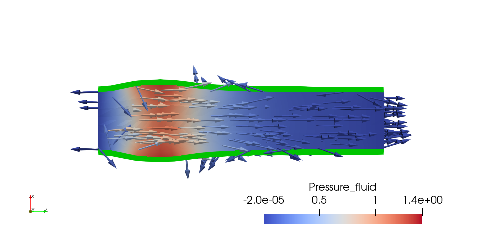
(a) $t=0.004s$

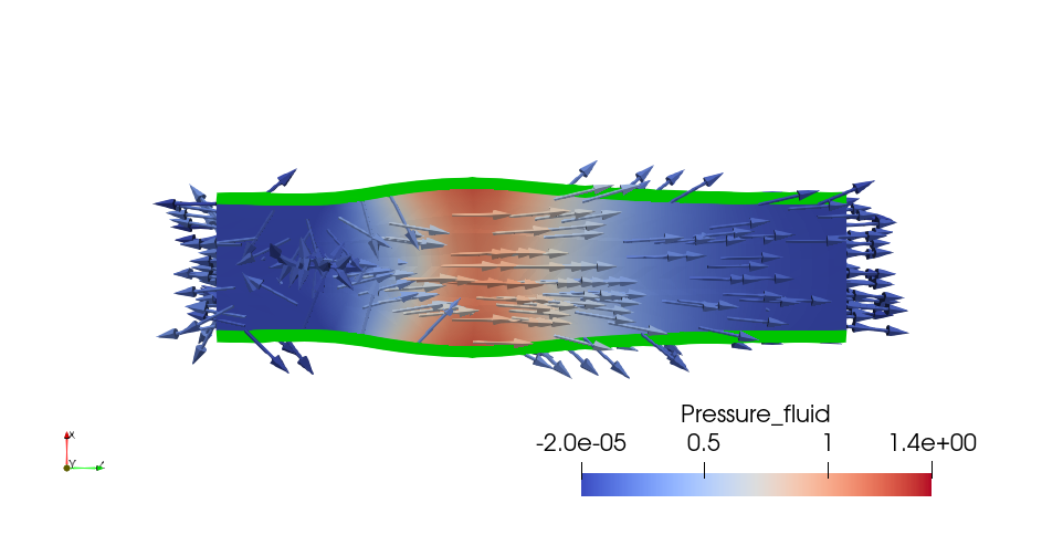
(b) $t=0.006s$

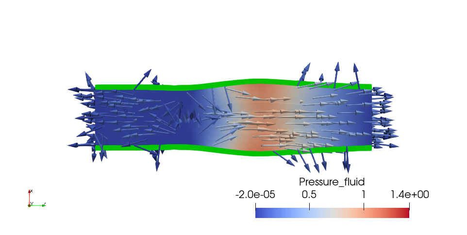
(c) $t=0.008s$

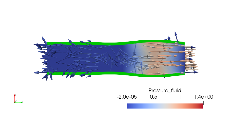
(d) $t=0.01s$

Figure 2: Pressure wave: middle cross-section velocity field, pressure distribution, velocity vectors and 10-fold enlarged structure displacement for several time instances.

The problem configuration consists of an incompressible viscous flow through a poroelastic tube with circular cross-section. The tube is $50$mm long, it has inner radius of $5$mm and the wall thickness is $1$mm. The fluid density is $10^{-3}$g/mm³ and kinematic viscosity is $3$mm²/s. The wall density $\rho_{s}$ is $1.2\cdot 10^{-3}$g/mm³. In (22), the Saint Venant–Kirchhof hyperelastic model is used with elastic modulus $E=3\cdot 10^{5}$g/mm/s² and Poisson’s ratio $\nu=0.3$. Initially, the fluid is at rest and the tube is non-deformed. The tube is fixed at both ends.

For the porous media parameters, we used porosity $\phi=0.3$ [13], mass storativity $s_{0}=5\cdot 10^{-5}mm\cdot s^{2}/g$ and two cases of the scalar permeability coefficient: $K=5\cdot 10^{-13}mm^{2}$ and $K=10^{-5}mm^{2}$. The smaller value mimics permeability estimated in rat’s cardiovascular system [13], while the larger value is taken from [25].

On the left open boundary of the tube, the external pressure $p_{ext}$ is set to $1.333\cdot 10^{3}$Pa for $t\in(0,3\cdot 10^{-3})$s and zero afterwards, while on the right open boundary the external pressure $p_{ext}$ is zero throughout the experiment. This generates a pressure impulse that travels along the tube. The external pressure is incorporated into (23)–(24) through the open boundary condition $\mbox{\boldmath$\sigma$\unboldmath}_{f}\mathbf{F}^{-T}\mathbf{n}=p_{ext}\mathbf{n}$.

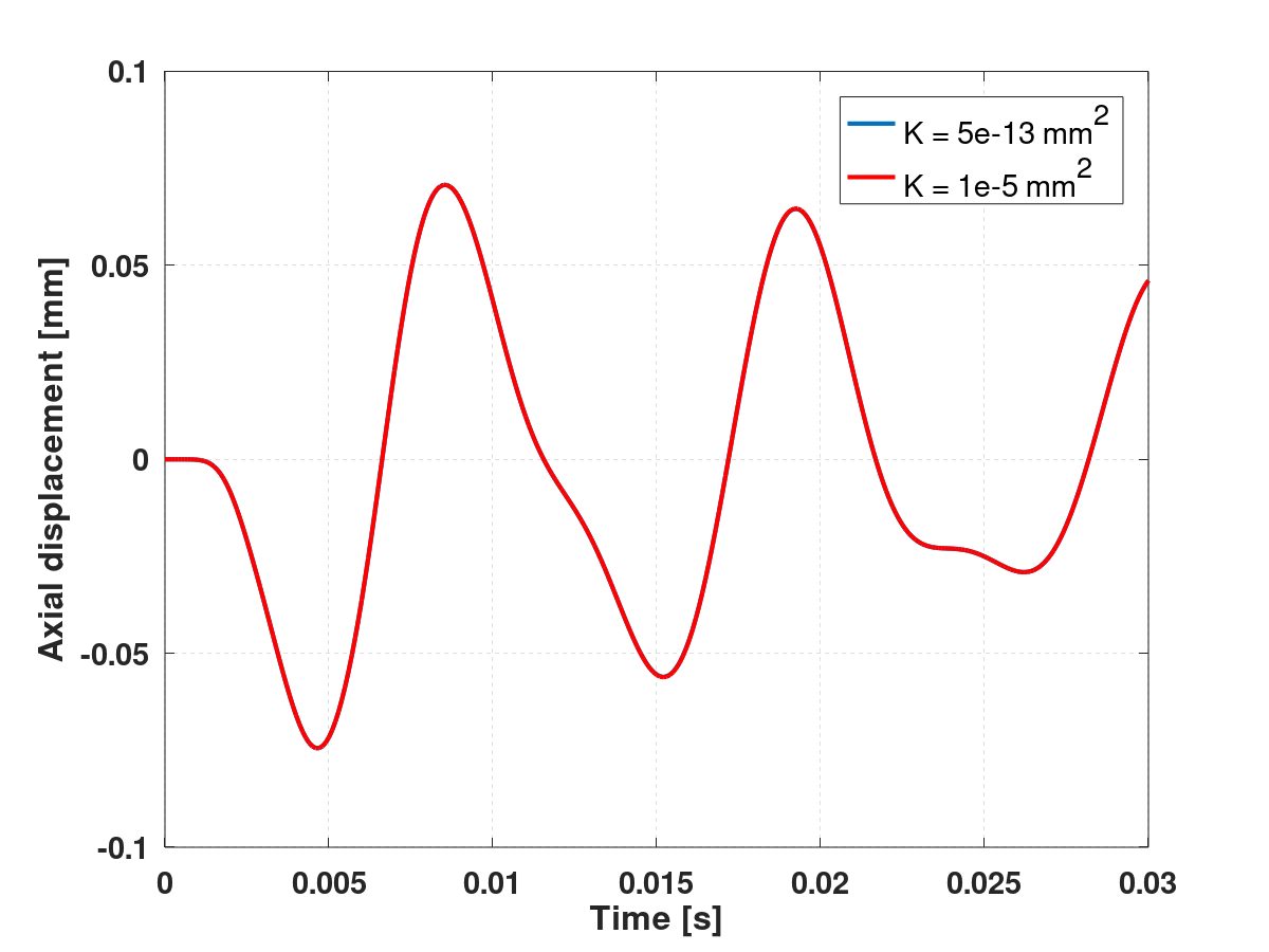
(a) axial component

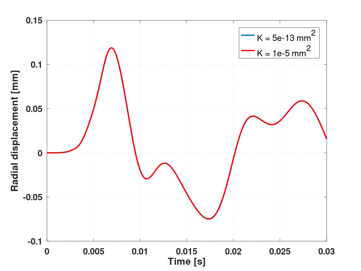
(b) radial component

Figure 3: Pressure wave: The axial and radial components of displacement of the inner tube wall at half the length of the pipe. Solutions are shown for the two cases of permeability (see the text). The plots are visibly indistinguishable.

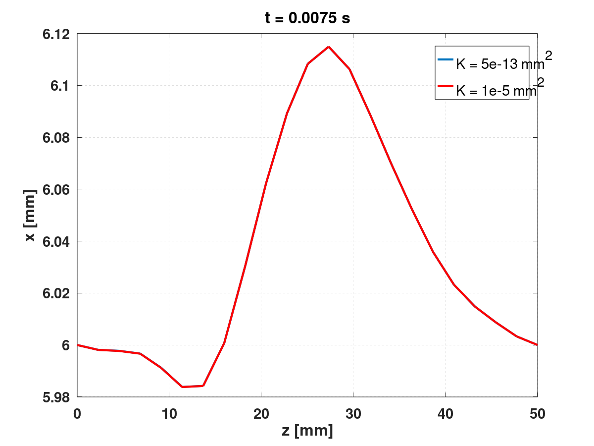
(a) $t=0.004s$

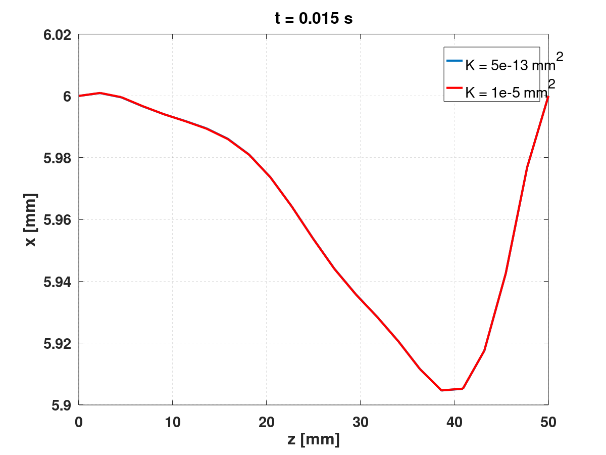
(b) $t=0.006s$

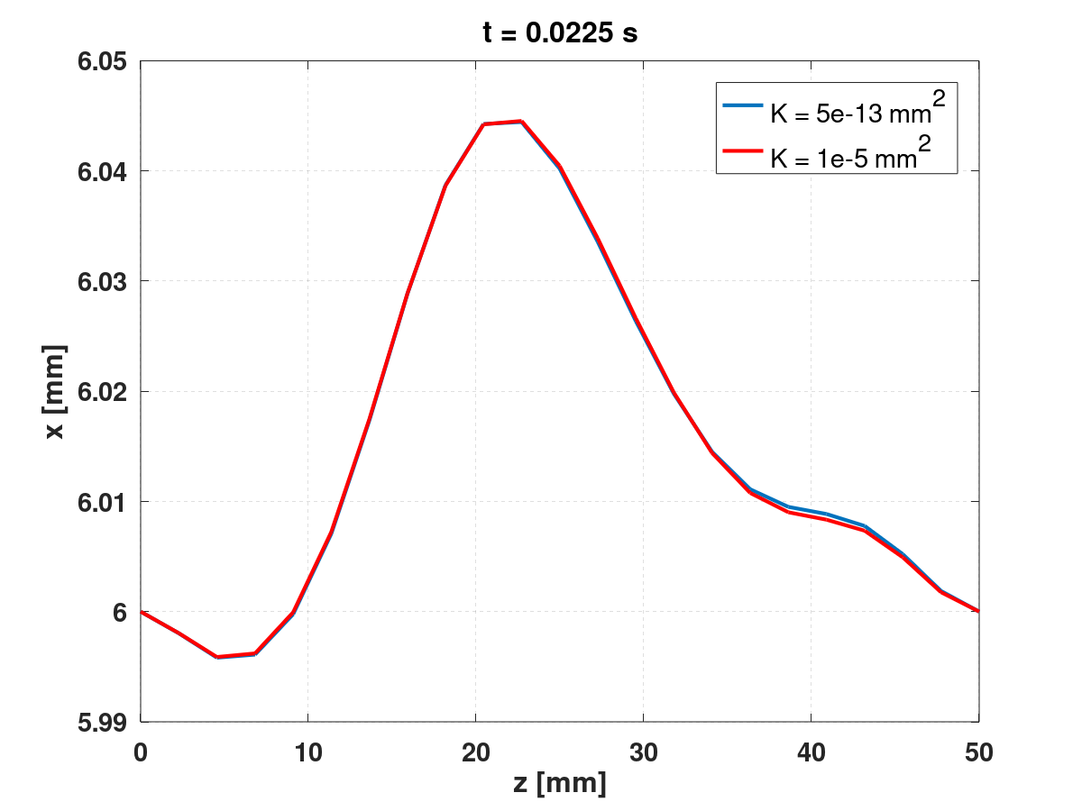
(c) $t=0.008s$

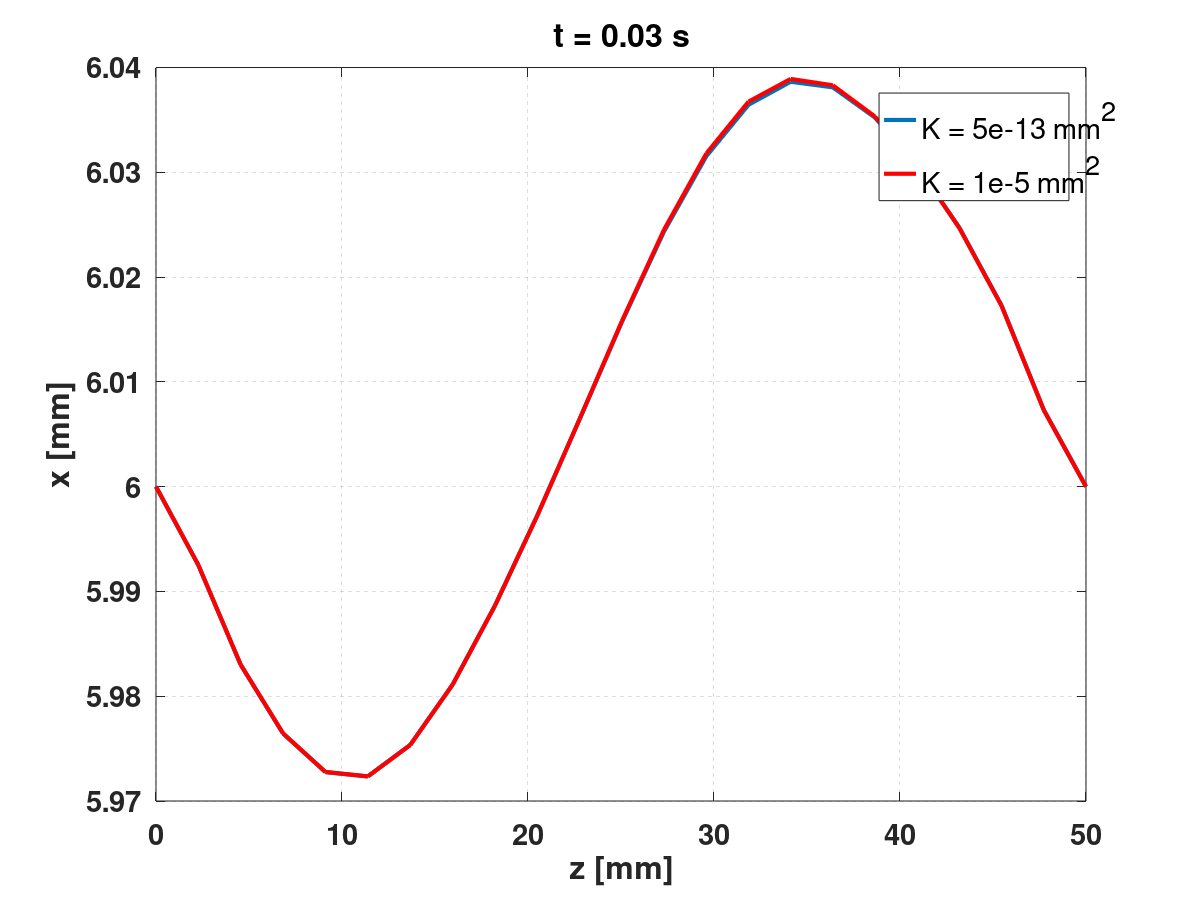
(d) $t=0.01s$

Figure 4: Wall profile on the outer side along the tube length for several time instances.

We use the Taylor–Hood P2-P1 elements for velocity and pressure variables and P2 elements for displacements, with the first order semi-implicit Euler discretization. The scheme (23)–(24) is implemented on the basis of the open source package Ani3D [26]. The important feature of equation (23) is linearization on each time step due to extrapolation of all geometric factors and the advection velocity from the previous time steps. The resulting linear system is solved by the multifrontal sparse direct solver MUMPS [3].

The conformal mesh used for the numerical experiment has 13200 and 6336 tetrahedra for the fluid and solid subdomains, yielding 340586 degrees of freedom. We set $\Delta t=10^{-4}$s, $\gamma=1$, $\tau=h^{-2}$ where $h$ is the local mesh size.

Figure 2 depicts the computed fluid velocity field in the middle cross-section and wall displacement exaggerated by a factor of 10 for clarity. The redder the color of the arrow is, the larger magnitude the velocity vector has.

Figure 3 shows the time variations of the radial and axial components of the displacement of the inner tube wall at half the length of the pipe, while Figure 4 shows the wall profile due to deformation at time instances $0.004,0.006,0.008,0.01$. Both Figures suggest that the difference in the permeabilities in this FPSI simulation scenario does not influence the FSI dynamics of the system.

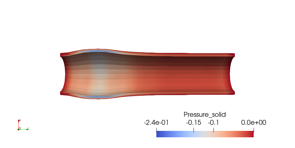
(a) $t=0.004s$

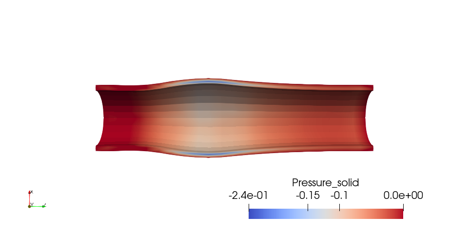
(b) $t=0.006s$

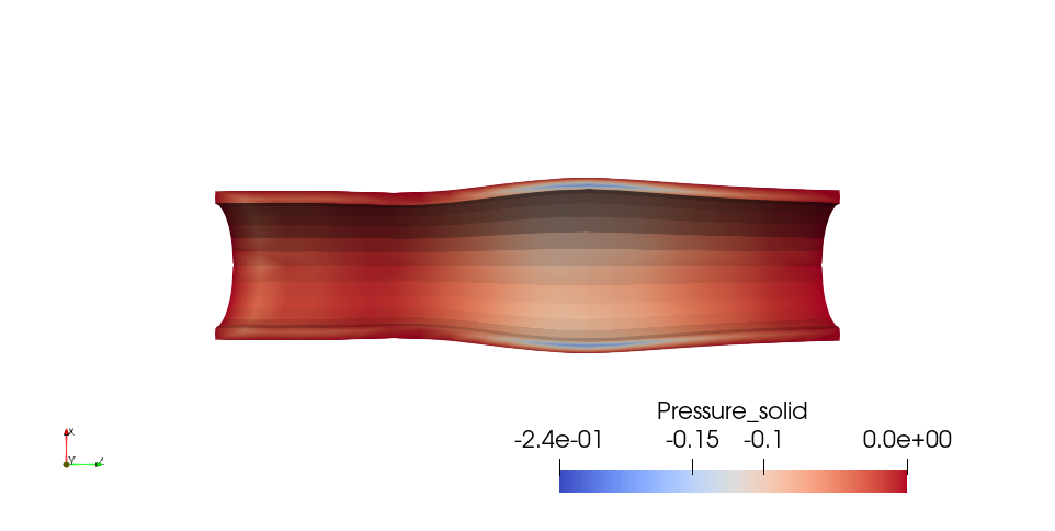
(c) $t=0.008s$

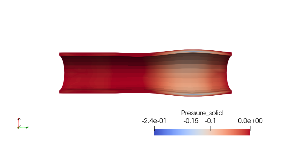
(d) $t=0.01s$

Figure 5: Porous pressure $p_{d}$ distribution in the solid: middle cross-section view, with 10-fold enlarged structure displacement for several time instances.

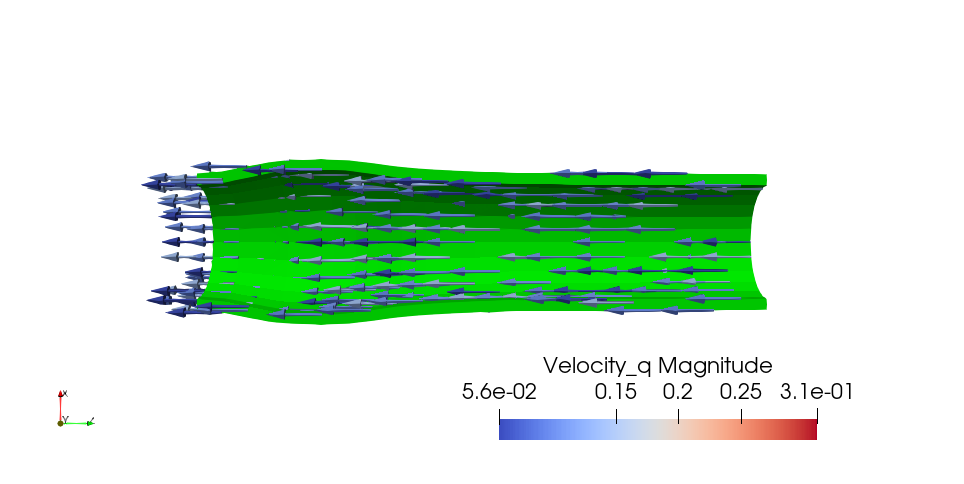
(a) $t=0.004s$

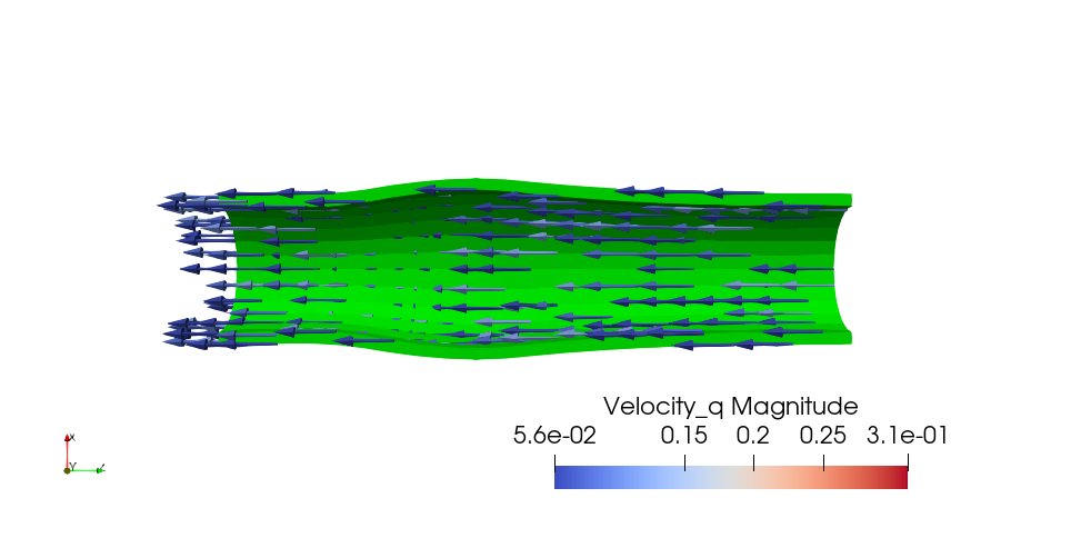
(b) $t=0.006s$

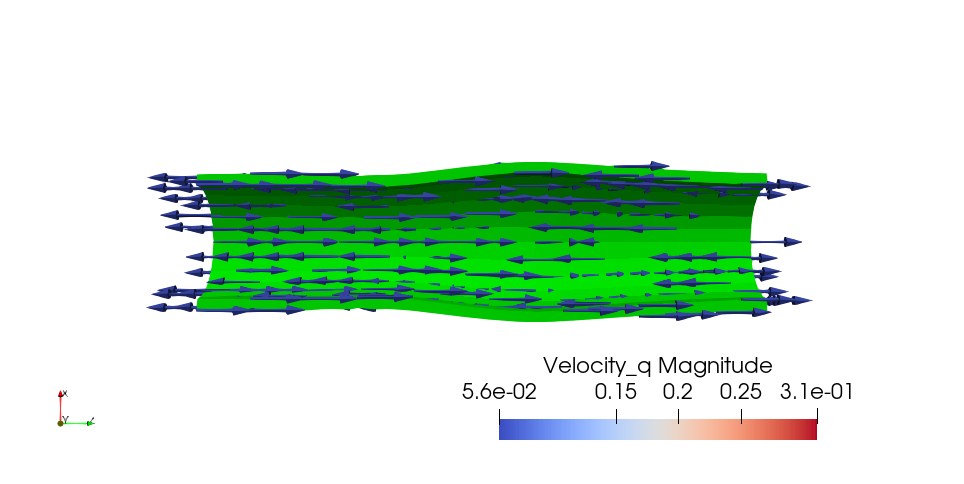
(c) $t=0.008s$

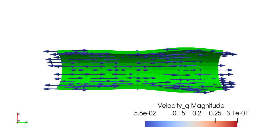
(d) $t=0.01s$

Figure 6: Filtration velocity $\mathbf{q}$ distribution in the solid: middle cross-section view, with 10-fold enlarged structure displacement for several time instances.

Figures 5-6 demonstrate the porous pressure and filtration velocity distributions for the same time instances $0.004,0.006,0.008,0.01$ and permeability $K=5\cdot 10^{-13}mm^{2}$. The maximum relative deviation for filtration velocity $\mathbf{q}$ between the two permeability cases approaches 35%: the smaller permeability is, the larger magnitude of $\mathbf{q}$. Both cases provide almost zero values for the non-axial components of $\mathbf{q}$. The axial component of $\mathbf{q}$ points against the direction of the pressure pulse wave along the entire tube length. The maximum relative deviation for the porous pressure $p_{d}$ is much lower, no more than 2.1%. The porous pressure is negative all across the tube wall and reaches zero value on the non-interface boundary according to the prescibed boundary conditions.

References

[1]
Christoph Ager, Benedikt Schott, Magnus Winter, and Wolfgang A Wall.
A Nitsche-based cut finite element method for the coupling of
incompressible fluid flow with poroelasticity.
Computer Methods in Applied Mechanics and Engineering,
351:253–280, 2019.
[2]
Ilona Ambartsumyan, Eldar Khattatov, Ivan Yotov, and Paolo Zunino.
A Lagrange multiplier method for a Stokes–Biot
fluid–poroelastic structure interaction model.
Numerische Mathematik, 140(2):513–553, 2018.
[3]
P.R. Amestoy et al.
MUMPS (MUltifrontal Massively Parallel sparse direct Solver).
http:mumps-consortium.org.
[4]
Lori Badea, Marco Discacciati, and Alfio Quarteroni.
Numerical analysis of the Navier–Stokes/Darcy coupling.
Numerische Mathematik, 115(2):195–227, 2010.
[5]
Santiago Badia, Annalisa Quaini, and Alfio Quarteroni.
Coupling Biot and Navier–Stokes equations for modelling
fluid–poroelastic media interaction.
Journal of Computational Physics, 228(21):7986–8014, 2009.
[6]
Y Bazilevs, JR Gohean, TJR Hughes, RD Moser, and Y Zhang.
Patient-specific isogeometric fluid–structure interaction analysis
of thoracic aortic blood flow due to implantation of the Jarvik 2000 left
ventricular assist device.
Computer Methods in Applied Mechanics and Engineering,
198(45-46):3534–3550, 2009.
[7]
Malte Braack and Piotr Boguslaw Mucha.
Directional do-nothing condition for the Navier-Stokes equations.
Journal of Computational Mathematics, pages 507–521, 2014.
[8]
M Bukač, Ivan Yotov, Rana Zakerzadeh, and Paolo Zunino.
Partitioning strategies for the interaction of a fluid with a
poroelastic material based on a Nitsche’s coupling approach.
Computer Methods in Applied Mechanics and Engineering,
292:138–170, 2015.
[9]
Martina Bukac, Ivan Yotov, Rana Zakerzadeh, and Paolo Zunino.
Effects of poroelasticity on fluid-structure interaction in arteries:
A computational sensitivity study.
In Modeling the heart and the circulatory system, pages
197–220. Springer, 2015.
[10]
A Çeşmelioğlu and Béatrice Rivière.
Analysis of time-dependent Navier–Stokes flow coupled with
Darcy flow.
Journal of Numerical Mathematics, 16:249–280, 2008.
[11]
Aycil Cesmelioglu, Vivette Girault, and Béatrice Riviere.
Time-dependent coupling of Navier–Stokes and Darcy flows.
ESAIM: Mathematical Modelling and Numerical Analysis,
47(2):539–554, 2013.
[12]
Ayçıl Çeşmelioğlu and Béatrice Rivière.
Primal discontinuous Galerkin methods for time-dependent coupled
surface and subsurface flow.
Journal of Scientific Computing, 40(1):115–140, 2009.
[13]
KY Chooi, A Comerford, SJ Sherwin, and PD Weinberg.
Intimal and medial contributions to the hydraulic resistance of the
arterial wall at different pressures: a combined computational and
experimental study.
Journal of The Royal Society Interface, 13(119):20160234, 2016.
[14]
Joris Degroote, Robby Haelterman, Sebastiaan Annerel, Peter Bruggeman, and Jan
Vierendeels.
Performance of partitioned procedures in fluid–structure
interaction.
Computers & structures, 88(7-8):446–457, 2010.
[15]
Ali Eken and Mehmet Sahin.
A parallel monolithic algorithm for the numerical simulation of
large-scale fluid structure interaction problems.
International Journal for Numerical Methods in Fluids,
80(12):687–714, 2016.
[16]
Luca Formaggia, Jean-Frédéric Gerbeau, Fabio Nobile, and Alfio
Quarteroni.
On the coupling of 3D and 1d Navier–Stokes equations for flow
problems in compliant vessels.
Computer methods in applied mechanics and engineering,
191(6-7):561–582, 2001.
[17]
Michael W Gee, Ulrich Küttler, and Wolfgang A Wall.
Truly monolithic algebraic multigrid for fluid–structure
interaction.
International Journal for Numerical Methods in Engineering,
85(8):987–1016, 2011.
[18]
Jean-Frédéric Gerbeau and Marina Vidrascu.
A quasi-Newton algorithm based on a reduced model for
fluid-structure interaction problems in blood flows.
ESAIM: Mathematical Modelling and Numerical Analysis,
37(4):631–647, 2003.
[19]
Vivette Girault and Béatrice Rivière.
Dg approximation of coupled Navier–Stokes and Darcy equations
by Beaver–Joseph–Saffman interface condition.
SIAM Journal on Numerical Analysis, 47(3):2052–2089, 2009.
[20]
J. Hron and S. Turek.
A monolithic FEM/multigrid solver for an ALE formulation of
fluid-structure interaction with applications in biomechanics.
Springer Berlin Heidelberg, 2006.
[21]
Trygve Karper, Kent-Andre Mardal, and Ragnar Winther.
Unified finite element discretizations of coupled Darcy–Stokes
flow.
Numerical Methods for Partial Differential Equations: An
International Journal, 25(2):311–326, 2009.
[22]
Nobuko Koshiba, Joji Ando, Xian Chen, and Toshiaki Hisada.
Multiphysics simulation of blood flow and LDL transport in a
porohyperelastic arterial wall model.
Journal of biomechanical engineering, 129(3):374–385, 2007.
[23]
Ulrich Küttler and Wolfgang A Wall.
Fixed-point fluid–structure interaction solvers with dynamic
relaxation.
Computational Mechanics, 43(1):61–72, 2008.
[24]
Mikel Landajuela, Marina Vidrascu, Dominique Chapelle, and Miguel A
Fernández.
Coupling schemes for the FSI forward prediction challenge:
comparative study and validation.
International journal for numerical methods in biomedical
engineering, 33(4), 2017.
[25]
Tongtong Li, Xing Wang, and Ivan Yotov.
Non-Newtonian and poroelastic effects in simulations of arterial
flows.
arXiv preprint arXiv:2010.14072, 2020.
[26]
K. Lipnikov, Yu. Vassilevski, A. Danilov, et al.
Advanced Numerical Instruments 3D.
http://sourceforge.net/projects/ani3d.
[27]
Alexander Lozovskiy, Maxim A Olshanskii, Victoria Salamatova, and Yuri V
Vassilevski.
An unconditionally stable semi-implicit FSI finite element method.
Computer Methods in Applied Mechanics and Engineering,
297:437–454, 2015.
[28]
Alexander Lozovskiy, Maxim A Olshanskii, and Yuri V Vassilevski.
Analysis and assessment of a monolithic FSI finite element method.
Computers & Fluids, 179:277–288, 2019.
[29]
AG Malan and Oliver F Oxtoby.
An accelerated, fully-coupled, parallel 3D hybrid finite-volume
fluid–structure interaction scheme.
Computer Methods in Applied Mechanics and Engineering,
253:426–438, 2013.
[30]
Ralph E Showalter.
Poroelastic filtration coupled to Stokes flow.
Lecture Notes in Pure and Applied Mathematics, 242:229, 2005.
[31]
Jing Wen and Yinnian He.
A strongly conservative finite element method for the coupled
Stokes–Biot model.
Computers & Mathematics with Applications, 80(5):1421–1442,
2020.