Carbonaceous sulfur hydride system: the strong-coupled room-temperature superconductor with a low value of Ginzburg-Landau parameter

Abstract

The superconducting state in Carbonaceous Sulfur Hydride (C-S-H) system is characterized by the record-high critical temperature of $288$ K experimentally observed at $\sim$267 GPa. Herein, we determined the properties of the C-S-H superconducting phase within the scope of both classical Eliashberg equations (CEE) and the Eliashberg equations with vertex corrections (VCEE). We took into account the scenarios pertinent to either the intermediate or the high value of electron-phonon coupling constant ($\lambda\sim 0.75$ or $\lambda\sim 3.3$, respectively). The scenario for the intermediate value, however, cannot be actually realized due to the anomally high value of logarithmic phonon frequency ($\omega_{\rm ln}/k_{B}=7150$ K) it would require. On the other hand, we found it possible to reproduce correctly the value of $T_{C}$ and other thermodynamic quantities in the case of strong coupling. However, the vertex corrections lower the order parameter values within the range from $\sim 50$ K to $\sim 275$ K. For the upper critical field $H_{C2}\sim 27$ T, the Ginzburg-Landau parameter $\kappa$ is of the order of $1.7$. This correlates well with the sharp drop of resistance observed by Hirsch and Marsiglio at the critical temperature. The strong-coupling scenario for C-S-H system is also suggested by the high values of $\lambda$ estimated for ${\rm H_{3}S}$ ($\lambda\sim 2.1$, $\kappa\sim 1.5$), ${\rm LaH_{10}}$ ($\lambda\sim 2.8$-$3.9$, $\kappa\sim 1.6$), and ${\rm YH_{6}}$ ($\lambda\sim 1.7$, $\kappa\sim 1.3$) compounds.

According to the Ashcroft thesis from 1968 Ashcroft (1968), hydrogen exposed to extremely high pressure should turn into metal and become the high-temperature superconductor. However, due to the metalization pressure greater than $500$ GPa, these predictions have not been verified experimentally yet McMahon et al. (2012); Dias and Silvera (2017). In 2004, Ashcroft pointed to the possibility of obtaining stable structures with properties similar to the metallic hydrogen, but achieved at significantly lower pressure, by adding atoms of heavier elements to hydrogen and inducing the effect of chemical pre-compression Ashcroft (2004). The first experiment confirming these theoretical predictions Duan et al. (2014) was conducted for $\rm{H_{3}S}$ compound, which electrical resistance drops to zero at $203$ K under the pressure of $155$ GPa Drozdov et al. (2015, 2014). This discovery led to the increase of interest in hydrogen-rich compounds, resulting in many theoretical papers. The most distinctive compounds described later are: $\rm{YH_{10}}$ ($T_{C}=326$ K, $250$ GPa) Liu et al. (2017), $\rm{LaH_{10}}$ ($T_{C}=288$ K, $200$ GPa) Peng et al. (2017), $\rm{ThH_{10}}$ ($T_{C}=241$ K, $100$ GPa) Kvashnin et al. (2018), and $\rm{ScH_{9}}$ ($T_{C}=233$ K, $300$ GPa) Ye et al. (2018). Among the above systems, $\rm{ThH_{10}}$ and $\rm{LaH_{10}}$ have been experimentally tested with the result: $\left[T_{C}\right]_{\rm{ThH_{10}}}=161$ K ($175$ GPa) Semenok et al. (2020) and $\left[T_{C}\right]_{\rm{LaH_{10}}}=250$-$260$ K ($170$-$200$ GPa) Drozdov et al. (2019); Somayazulu et al. (2019).

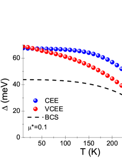
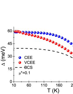
Figure 1: The order parameter as a function of temperature for C-S-H, ${\rm LaH_{10}}$ and ${\rm YH_{6}}$ systems, respectively. The results were obtained from the classical Eliashberg equations (CEE) and the Eliashberg equations with vertex corrections (VCEE). The colored spheres represent the numerical data. The dashed lines are the BCS predictions.

The latest experimental data obtained for the C-S-H system under the pressure of $267\pm 10$ GPa prove the existence of the superconducting state characterized by the record-high value of critical temperature ($T_{C}=287.7$$\pm 1.2$ K). This temperature noticeably exceeds the superconducting transition temperature obtained for the ${\rm H_{3}S}$ Drozdov et al. (2015, 2014) and the ${\rm{LaH_{10}}}$ Somayazulu et al. (2019); Drozdov et al. (2019) compounds. The C-S-H system exhibits superconducting properties over a wide range of pressure, from about $140$ GPa to about $275$ GPa. For the lowest pressure, the critical temperature is equal to $147$ K and then increases gradually. Near the pressure of $225$ GPa, the characteristic inflection of $T_{C}\left(p\right)$ is observed, which may be related to the structural transition. Above the pressure of $225$ GPa, the increase in critical temperature is very fast. The maximum value of $T_{C}\sim 288$ K was observed at the pressure of $\sim 267$ GPa Snider et al. (2020).

It is suspected that the superconducting state in the C-S-H system is induced by the electron-phonon interaction, as in the strongly-coupled systems ${\rm H_{3}S}$ ($\left[\lambda\right]_{\rm H_{3}S}\sim 2$) Duan et al. (2014); Durajski et al. (2016) and ${\rm{LaH_{10}}}$ ($\left[\lambda\right]_{\rm LaH_{10}}\sim 3$) Liu et al. (2017); Kruglov et al. (2020). The above hypothesis is in line with the recent results obtained with help of DFT calculations. In particular, Hu et. al Hu et al. (2020) showed that the enhancement of electron-phonon coupling can be induced in compounds such as ${\rm C_{1}S_{15}H_{48}}$ and ${\rm C_{1}S_{17}H_{54}}$ by replacing a small amount of sulfur atoms with carbon. At the same time, this results in the higher averaged phonon frequency, which increases with pressure. As a result, the critical temperature reaches the value of the room temperature at $270$ GPa. Additionally, the calculations of critical temperature of both ${\rm C_{1}S_{15}H_{48}}$ and ${\rm C_{1}S_{17}H_{54}}$, regarded as the function of pressure, are in good agreement with the experimental data Snider et al. (2020). However, according to the Hirsch and Marsiglio’s observation Hirsch and Marsiglio (2020), confirmed also by Dogan and Cohen Dogan and Cohen (2020), the sharp change in C-S-H resistance at superconducting transition Snider et al. (2020) may indicate that the recorded results mirror some physical mechanisms not related to the superconductivity. Worse still, the same argument can be given for compounds such as ${\rm H_{3}S}$ and ${\rm LaH_{10}}$.

The aim of the presented work is the thorough analysis of Hirsch and Marsiglio’s argument on the basis of correctly determined thermodynamic properties of the C-S-H, ${\rm H_{3}S}$, ${\rm LaH_{10}}$, and ${\rm YH_{6}}$ compounds. Let us begin with introducing the reasoning adopted by these authors.

Snider et. al Snider et al. (2020), apart from finding the critical temperature of the C-S-H system, estimated also the upper critical field $H_{C2}$. It was shown within the Ginzburg-Landau (GL) approach that $H_{C2}\left(0\right)=61.88$ T, with the Pippard coherence length of $\zeta\left(0\right)=2.31$ nm. For the conventional Werthamer-Helfand-Hohenberg (WHH) approach (the dirty limit), the value of $H_{C2}(0)=85.34$ T was extrapolated from the slope of the $H$-$T$ curve as: $H_{C2}\left(0\right)=0.693T_{C}|\frac{dH_{C2}}{dT}|_{T=T_{C}}$. The coherence length $\zeta\left(0\right)$ is equal to $1.96$ nm in this case. For both the GL and the WHH models, the coherence length was calculated from the formula: $\zeta\left(0\right)=\left[\phi_{0}/2\pi H_{C2}\left(0\right)\right]^{1/2}$, where $\phi_{0}=h/2e=2.068\cdot 10^{-15}$ Wb is the flux quantum. Hirsch and Marsiglio noticed Hirsch and Marsiglio (2020) that the value of the London penetration depth ($\lambda_{L}\left(0\right)=3.8$ nm Snider et al. (2020)) was calculated incorrectly. The correctly made estimation of $\lambda_{L}\left(0\right)$ within the GL and BCS model gives $113$ nm. This may suggest that C-S-H is the strongly type-II superconductor with the Ginzburg-Landau parameter $\kappa=\lambda_{L}\left(0\right)/\zeta\left(0\right)$ of $\sim 50$. Therefore it can be placed between the cuprate superconductors ($\kappa\sim 100$) and ${\rm MgB_{2}}$ ($\kappa\sim 28$). If so, the sharp drop in resistance observed at the critical temperature cannot be related to superconducting transition, because such a drop in resistance exhibited by the strongly type-II superconductors is evidently milder - especially in the external magnetic field - see for example the data reported for ${\rm MgB_{2}}$ Canfield et al. (2003), YBCO Iye et al. (1988), or NbN Hazra et al. (2016).

In the folowing paragraphs, we report our results to show that Hirsch and Marsiglio’s argument is incorrect due to the fact that their calculations Hirsch and Marsiglio (2020) were carried out by using the weak-coupling model.

Firstly, we proved that the C-S-H system belongs to the group of superconductors with the high value of coupling constant $\lambda$. Hence it follows that its thermodynamic properties can be correctly reproduced within the Eliashberg formalism (the strong-coupling approach) Eliashberg (1960); Migdal (1958); Carbotte (1990); Freericks et al. (1997) (Suppl. I and Suppl. II). Secondly, taking into account the observed sharp drop in C-S-H resistance at the critical temperature, it was assumed that the superconducting phase of the discussed system is characterized by the low value of the Ginzburg-Landau parameter. It should be noted that this scenario is in line with predictions of the Eliashberg formalism.

The thermodynamic properties of the C-S-H system in the superconducting state were calculated for both the intermediate-coupling ($\lambda=0.75$) and the strong-coupling ($\lambda=3.26$) approach (Suppl. III and Suppl. IV). The logarithmic phonon frequency $\omega_{\rm ln}$ was estimated using the formula Mitrovic et al. (1984): $R_{\Delta}=3.53\left[1+12.5\left[T_{C}/\omega_{\rm ln}\right]^{2}\ln\left(\omega_{\rm ln}/2T_{C}\right)\right]$. The dimensionless ratio $R_{\Delta}$ was calculated within the Eliashberg approach (see Tab. I in Suppl. III). The critical temperature $T_{C}=287.7$ K was taken from the experiment Snider et al. (2020). For the intermediate coupling, we obtained $\omega_{\rm ln}/k_{B}=7150$ K. This anomally high value precludes the scenario of the intermediate (or weak) electron-phonon coupling in the case of the C-S-H system. In the strong-coupling case, the ratio $\omega_{\rm ln}/k_{B}$ is equal to $1130$ K. Similar values of $\omega_{\rm ln}/k_{B}$ ($800$-$1600$ K) were obtained also for the ${\rm H_{2}S}$, ${\rm H_{3}S}$, ${\rm LaH_{10}}$, and ${\rm YH_{6}}$ compounds (Suppl. V). Please note the parameter $r=k_{B}T_{C}/\omega_{\rm ln}$, which characterizes retardation and strong-coupling effects. The value of $r$ equals $0.04$ for $\lambda=0.75$ (in the BSC limit $r=0$), and it reaches $0.25$ in the case of strong-coupling. Thus the deviation from the prediction of BCS theory is clearly visible.

Table 1: The values of upper critical field for the C-S-H system in the superconducting state ($p=267$ GPa). Results obtained by using the CEE model for the intermediate-coupling and the strong-coupling cases.

$\lambda$	$\omega_{\rm ln}/k_{B}$ (K)	$h^{cl}_{C2}\left(0\right)$	$H^{cl}_{C2}\left(0\right)$ (T)	$h^{di(1)}_{C2}\left(0\right)$	$H^{di(1)}_{C2}\left(0\right)$ (T)	$h^{di(2)}_{C2}\left(0\right)$	$H^{di(2)}_{C2}\left(0\right)$ (T)
0.75	7150.5	0.72631	89.44	0.65603	80.79	0.66157	81.47
3.26	1130.5	0.93388	115	0.56886	70.0	0.22370	27.5

The upper critical field at zero Kelvin was estimated by the formula Carbotte (1990): $H_{C2}\left(0\right)=\eta\left(T_{C}\right)h_{C2}\left(0\right)$, where the coefficient $\eta\left(T_{C}\right)=T_{C}|\frac{dH_{C2}(T)}{dT}|_{T_{C}}|$ was calculated on the basis of experimental data Snider et al. (2020). We identified the value of $h_{C2}\left(0\right)$ in the clean (cl) and dirty (di) limit. In the cl case, the formula for $h_{C2}\left(0\right)$ takes the form Carbotte (1990): $h^{cl}_{C2}\left(0\right)=0.727\left[1-2.7\left[T_{C}/\omega_{\rm ln}\right]^{2}\ln\left(\omega_{\rm ln}/20T_{C}\right)\right]$. For the dirty limit, two expressions were given Carbotte (1990), that represent the limits within which the experimental data should fall: $h^{di(1)}_{C2}\left(0\right)=0.69\left[1-1.5T_{C}/\omega_{\rm ln}+2\left[T_{C}/\omega_{\rm ln}\right]^{2}\ln\left(\omega_{\rm ln}/0.8T_{C}\right)\right]$, and $h^{di(2)}_{C2}\left(0\right)=0.69\left[1-T_{C}/\omega_{\rm ln}+3.2\left[T_{C}/\omega_{\rm ln}\right]^{2}\ln\left(\omega_{\rm ln}/30T_{C}\right)\right]$. We obtained the results which are collected in Tab. 1. It is clearly visible that, for the intermediate coupling, the theoretical values of upper critical field ($H^{di(1)}_{C2}\left(0\right)=80.79$ T and $H^{di(1)}_{C2}\left(0\right)=81.47$ T) agree qualitatively with the Snider’s data: $H_{C2}(0)=85.34$ T (the WHH approach). This result should not come as a surprise, because in the case of intermediate coupling, the Eliashberg equations give results comparable to the BCS mean-field theory and related phenomenological models. However, as we already mentioned, the method of estimating the upper critical field based on the intermediate-coupling approach should be rejected due to the required anomally high value of logarithmic phonon frequency. In the strong-coupling limit, the upper critical field computed for the cl case has a very high value of $115$ T. It is hard to suppose, however, that this case would take place in such a complex system as C-S-H. In the dirty limit, the Eliashberg theory predicts a wide range of upper critical field, from $\sim 27.5$ T to $\sim 70$ T.

Table 2: The values of $\zeta$, $\lambda_{L}$ and $\kappa$ for the C-S-H system ($p=267$ GPa). Results obtained by using the CEE model for the intermediate-coupling and the strong-coupling cases.

$\lambda$	$\zeta^{di(1)}\left(0\right)$ (nm)	$\zeta^{di(2)}\left(0\right)$ (nm)	$\lambda_{L}^{di(1)}\left(0\right)$ (nm)	$\lambda_{L}^{di(2)}\left(0\right)$ (nm)	$\kappa^{di(1)}$	$\kappa^{di(2)}$
0.75	2.02	2.01	124.01	124.79	61.41	62.06
3.26	2.17	3.46	30.57	15.17	14.09	4.38

The computed values of the Pippard coherence length $\zeta\left(0\right)$, the London penetration depth $\lambda_{L}\left(0\right)=1935\left(\Delta\left(0\right)\zeta\left(0\right)\right)^{-3/2}\left(m_{e}/m_{e}^{\star}\right)$ Hirsch and Marsiglio (2020), and the Ginzburg-Landau parameter $\kappa$ are gathered in Tab. 2. The sharp change in resistance observed experimentally for C-S-H at the transition temperature strongly suggests that, for the system in question, one should take into account the low value of Ginzburg-Landau parameter of the order of $4$ (Tab. 2). Finally, the Ginzburg-Landau parameter for the Eliashberg approach can also be calculated directly from the formula Carbotte (1990): $\kappa=1.2\left[1+2.3\left[T_{C}/\omega_{\rm ln}\right]^{2}\ln\left(\omega_{\rm ln}/0.2T_{C}\right)\right]$. In this case, for the value of $\lambda$ befitting the strong-coupling, we get $\kappa=1.73$. The above result correlates well with $\kappa\sim 4$ obtained within the more qualitative approach.

The presented analysis of C-S-H properties is consistent with theoretical results based on the DFT method applied to the ${\rm C_{1}S_{15}H_{48}}$ and ${\rm C_{1}S_{17}H_{54}}$ systems Hu et al. (2020). Additionaly, it should be kept in mind that in all hydrogen-rich systems with high $T_{C}$, only the scenario of strong-coupling has been realized so far (Suppl. V). For example, the electron-phonon coupling constant $\lambda$ is of the order of $2$-$3$ in the case of ${\rm LaH_{10}}$ Kostrzewa et al. (2020); Kruglov et al. (2020) (Suppl. VI), and it was found to be $\sim 2$ for ${\rm H_{3}S}$ Duan et al. (2014); Durajski et al. (2016). Let us also mention that another experimental detection of high-temperature superconducting state was recently reported Troyan et al. (2021), this time in the $\rm YH_{6}$ compound ($T_{C}=224$ K at $166$ GPa). We provided the detailed description of ${\rm YH_{6}}$ properties by using the classical Eliashberg equations (CEE) and the Eliashberg equations with vertex corrections (VCEE) (Suppl. VII). It turns out that the estimated value of electron-phonon coupling constant for $\rm YH_{6}$ is also relatively high and amounts to $1.71$ Troyan et al. (2021).

In the considered cases, the correctly calculated values of Ginzburg-Landau parameter are: $\left[\kappa\right]_{{\rm LaH_{10}}}=1.60$ ($T_{C}=260$ K; $p=190$ GPa), $\left[\kappa\right]_{{\rm H_{3}S}}=1.53$ ($T_{C}=203$ K; $p=155$ GPa) and $\left[\kappa\right]_{{\rm YH_{6}}}=1.34$ ($T_{C}=224$ K; $p=166$ GPa), respectively.

The temperature dependence of order parameter determined within the CEE formalism distinctly differs from the predictions of BCS theory for all hydrogen-rich high-temperature superconductors (see Fig. 5). In addition, the vertex corrections are important for the region of intermediate temperature and lower the values of $\Delta\left(T\right)$. The low-temperature value of C-S-H order parameter $\Delta\left(0\right)$ is between $67.64$ meV and $68.94$ meV (Tab. I in Suppl. III). This means that the dimensionless ratio $R_{\Delta}=2\Delta\left(0\right)/k_{B}T_{C}$ is from $5.46$ to $5.56$. The electron effective mass at $T_{C}$ ranges from $2.69$ $m_{e}$ to $4.26$ $m_{e}$. The dimensionless parameters $R_{H}=T_{C}C^{N}\left(T_{C}\right)/H_{C}^{2}\left(0\right)$ and $R_{C}=\Delta C\left(T_{C}\right)/C^{N}\left(T_{C}\right)$ are equal to $0.177$ and $2.37$, respectively. Taking the above into account, it can be clearly shown by using experimental methods that the C-S-H system belongs to the family of superconductors with high value of electron-phonon coupling constant.

Hirsch and Marsiglio noted in their paper Hirsch and Marsiglio (2020) that for high values of electron-phonon coupling constant ($\lambda>2$) the Eliashberg formalism may not apply due to the formation of polarons. Please note, however, that the standard Eliashberg equations do not take into account all mechanisms that may contribute to the reduction of coupling constant. In particular, attention should be paid to anharmonic effects Errea et al. (2015), which should be taken into account both in the Eliashberg function and in the form of equations themselves. The many-body effects also play the significant role, lowering the value of $\lambda$, while the form of function $\Delta\left(T\right)$ does not change (Suppl. VIII). This means that the Eliashberg approach is, with high probability, sufficient to determine correctly the properties of hydrogen-rich high-temperature superconductors.

Summarizing, the conducted analysis showed that the superconducting state in the C-S-H system can be induced by strong electron-phonon interaction, as it is for the ${\rm LaH_{10}}$, ${\rm H_{3}S}$, and ${\rm YH_{6}}$ superconductors. For the C-S-H system, the Eliashberg formalism predicts that the value of Ginzburg-Landau parameter is low ($\kappa=1.73$). We got equally low values also in other cases, i.e. $\left[\kappa\right]_{{\rm LaH_{10}}}=1.60$, $\left[\kappa\right]_{{\rm H_{3}S}}=1.53$, and $\left[\kappa\right]_{{\rm YH_{6}}}=1.34$. This means that the experimental results obtained for hydrogen-rich compounds do not contradict the theory of superconducting state. Referring to the DFT-Eliashberg formalism, it should be strongly emphasized that this is the approach that allows for the correct prediction of properties of superconducting state before performing experimental measurements.

Supporting Information for: Carbonaceous sulfur hydride system: the strong-coupled room-temperature superconductor with a low value of Ginzburg-Landau parameter

I Classical Eliashberg formalism

Basic equations used to analyse the thermodynamic properties of superconducting state in high-pressure hydrogen-containing systems are the classical Eliashberg equations (CEE) Eliashberg (1960); Migdal (1958); Carbotte (1990). The mentioned formalism allows to take into account the retardation and strong-coupling effects related to linear electron-phonon interaction. Equally important is the fact that input parameters to the pairing kernel in Eliashberg equations can be calculated with high accuracy using the DFT method Parr and Yang (1989).

On imaginary axis ($i=\sqrt{-1}$), the classical Eliashberg equations take following form:

$$\varphi_{n}=\pi k_{B}T\sum_{m=-M}^{M}\frac{\lambda_{n,m}-\mu^{\star}\left(\omega_{m}\right)}{\sqrt{\omega_{m}^{2}Z_{m}^{2}+\varphi_{m}^{2}}}\varphi_{m},$$ (1)

$$Z_{n}=1+\pi k_{B}T\sum_{m=-M}^{M}\frac{\lambda_{n,m}}{\sqrt{\omega_{m}^{2}Z_{m}^{2}+\varphi_{m}^{2}}}\frac{\omega_{m}}{\omega_{n}}Z_{m},$$ (2)

where: $\varphi_{n}=\varphi_{n}(i\omega_{n})$ and $Z_{n}=Z(i\omega_{n})$ denote the order parameter function and the wave function renormalization factor, respectively. The order parameter is defined by: $\Delta_{n}=\varphi_{n}/Z_{n}$. The other symbols have the following meanings: $\omega_{n}$ is the $n$-th fermionic Matsubara frequency expressed by formula: $\omega_{n}=\pi k_{B}T(2n-1)$, where $k_{B}$ is the Boltzmann constant. The function $\mu^{\star}(\omega_{m})$ models depairing interaction between electrons: $\mu^{\star}(\omega_{m})=\mu^{\star}\theta(\Omega_{C}-|\omega_{m}|)$, $\mu^{\star}$ is the Coulomb pseudopotential Morel and Anderson (1962); Bauer et al. (2012), $\theta$ denotes the Heaviside function and $\Omega_{C}$ is so-called cut-off frequency. In numerical calculations, we have assumed $\Omega_{C}=1$ eV. The electron-phonon pairing kernel can be defined as follows:

$$\lambda_{n,m} = 2\int^{\omega_{D}}_{0}d\omega\frac{\alpha^{2}F\left(\omega\right)\omega}{\left(\omega_{n}-\omega_{m}\right)^{2}+\omega^{2}}=2\int^{\omega_{D}}_{0}d\omega\frac{\omega^{2}}{\left(\omega_{n}-\omega_{m}\right)^{2}+\omega^{2}}\frac{\alpha^{2}F\left(\omega\right)}{\omega}$$

$$\simeq \frac{\omega_{0}^{2}}{\left(\omega_{n}-\omega_{m}\right)^{2}+\omega_{0}^{2}}2\int^{\omega_{D}}_{0}d\omega\frac{\alpha^{2}F\left(\omega\right)}{\omega}=\lambda\frac{\omega_{0}^{2}}{\left(\omega_{n}-\omega_{m}\right)^{2}+\omega_{0}^{2}},$$

where: $\lambda=2\int^{\omega_{0}}_{0}d\Omega\frac{\alpha^{2}F\left(\Omega\right)}{\Omega}$, denotes the electron-phonon coupling constant, $\alpha^{2}F\left(\Omega\right)$ is the Eliashberg function and $\omega_{0}$ denotes the characteristic phonon frequency.

After determining the values of order parameter $\Delta_{n}$ and wave function renormalization factor $Z_{n}$, the following thermodynamic parameters of superconducting state can be calculated:

• The half-width of energy gap:

  $$\Delta\left(T\right)={\rm Re}\left[\Delta\left(\omega=\Delta\left(T\right)\right)\right],$$ (4)

  where $\Delta\left(\omega\right)$ is calculated by analytical continuation of the solutions of Eliashberg equations on real axis Beach et al. (2000). On this basis, the dimensionless ratio $R_{\Delta}=2\Delta\left(0\right)/k_{B}T_{C}$ is determined, where $\Delta(0)=\Delta\left(T_{0}\right)$. In the Fig. 2 for C-S-H, we presented the example form of order parameter and wave function renormalization factor on real axis. We have taken into account the lowest temperature: $T=T_{0}$. We can notice that order parameter is the complex function and in the range of lower frequencies, corresponding to physical values of energy gap, the non-zero is only Re$\left[\Delta\left(\omega\right)\right]$. From the physical point of view this result indicates the absence of damping effects, which are modeled by Im$\left[\Delta\left(\omega\right)\right]$. Based on presented data, it is also possible to calculate the quasiparticle density of states: $\frac{N^{S}(\omega)}{N^{N}(\omega)}={\rm Re}\left[\frac{\omega-i\Gamma}{\sqrt{\left(\omega-i\Gamma\right)^{2}-\Delta^{2}(\omega)}}\right]$, where the pair-breaking parameter $\Gamma$ equals $0.1$ meV. In Fig. 3, we plotted $N^{S}(\omega)/N^{N}(\omega)$ for the cases $\omega_{0}=\omega_{D}$ and $\omega_{0}=100$ meV. The characteristic maxima of $N^{S}\left(\omega\right)/N^{N}\left(\omega\right)$ are formed at the points $\omega=\pm\Delta$.

  

  

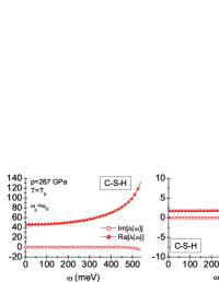
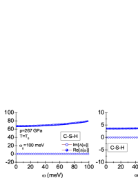
  Figure 2: The order parameter and the wave function renormalization factor on real axis for C-S-H ($p=267$ GPa and $T=T_{0}$). Results were obtained for $\omega_{0}=\omega_{D}$ and $\omega_{0}=100$ meV.

  

  

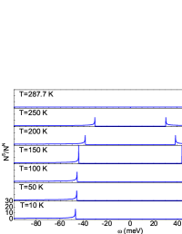
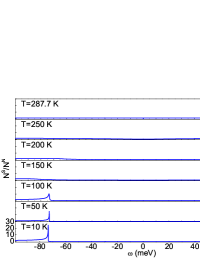
  Figure 3: The quasiparticle density of states for C-S-H ($p=267$ GPa). The results were obtained for $\omega_{0}=\omega_{D}$ and $\omega_{0}=100$ meV.

• The free energy difference between the superconducting and the normal state Carbotte (1990):

  $$\frac{\Delta F}{\rho\left(\varepsilon_{F}\right)}=-\frac{2\pi}{\beta}\sum_{n=1}^{M}\left(\sqrt{\omega^{2}_{n}+\Delta^{2}_{n}}-\left|\omega_{n}\right|\right)\left(Z^{S}_{n}-Z^{N}_{n}\frac{\left|\omega_{n}\right|}{\sqrt{\omega^{2}_{n}+\Delta^{2}_{n}}}\right),$$ (5)

  where $\rho\left(\varepsilon_{F}\right)$ denotes the electron density of states at the Fermi level. The symbols $Z^{S}_{n}$ and $Z^{N}_{n}$ represent the wave function renormalization factor for supercondacting ($S$) and normal ($N$) state, respectively. Note that from the physical point of view, the negative values of $\Delta F$ prove thermodynamic stability of the superconducting condensate. The first derivative of function given by Eq. (5) determines the entropy difference between superconducting and normal state ($\Delta S$). The negative values of $\Delta S$ prove that the entropy of superconducting state is lower than the entropy of normal state due to the existence of Cooper pairs (see Fig. 4).

  

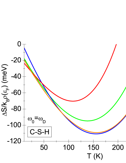
  Figure 4: The entropy difference between superconducting and normal state as a function of temperature for C-S-H. We took into account the selected pressure values and the case $\omega_{0}=\omega_{D}$.

• The thermodynamic critical field:

  $$\frac{H_{C}}{\sqrt{\rho\left(\varepsilon_{F}\right)}}=\sqrt{-8\pi\left[\Delta F/\rho\left(\varepsilon_{F}\right)\right]}.$$ (6)

• The specific heat difference between superconducting and normal state ($\Delta C=C^{S}-C^{N}$):

  $$\frac{\Delta C\left(T\right)}{k_{B}\rho\left(\varepsilon_{F}\right)}=-\frac{1}{\beta}\frac{d^{2}\left[\Delta F/\rho\left(\varepsilon_{F}\right)\right]}{d\left(k_{B}T\right)^{2}}.$$ (7)

  The specific heat of normal state is the most convenient to estimate by the formula:

  $$\frac{C^{N}\left(T\right)}{k_{B}\rho\left(\varepsilon_{F}\right)}=\frac{\gamma}{\beta},$$ (8)

  where Sommerfeld constant is given by: $\gamma=\frac{2}{3}\pi^{2}\left(1+\lambda\right)$.

  On the basis of results obtained for the thermodynamic critical field and the specific heat, it is also possible to calculate the values of dimensionless ratios:

  $$R_{H}=\frac{T_{C}C^{N}\left(T_{C}\right)}{H_{C}^{2}\left(0\right)},\qquad{\rm and}\qquad R_{C}=\frac{\Delta C\left(T_{C}\right)}{C^{N}\left(T_{C}\right)}.$$ (9)

II Eliashberg formalism including the vertex correction

We discuss formalism determining the effect of vertex corrections on thermodynamic properties of the superconducting state. Note that this type of analysis was carried out, among others, for the fullerene systems Pietronero and Strässler (1992); Pickett (1993), the high-$T_{C}$ cuprates Uemura et al. (1991, 1992); D’Ambrumenil (1991), the heavy fermion compounds Wojciechowski (1996) and in the superconductors under high magnetic fields Goto and Natsume (1996). In particular, the Eliashberg equations taking into account vertex corrections take the form Freericks et al. (1997):

$$\varphi_{n} = \pi k_{B}T\sum_{m=-M}^{M}\frac{\lambda_{n,m}-\mu_{m}^{\star}}{\sqrt{\omega_{m}^{2}Z^{2}_{m}+\varphi^{2}_{m}}}\varphi_{m}$$

$$- \frac{\pi^{3}\left(k_{B}T\right)^{2}}{4\varepsilon_{F}}\sum_{m=-M}^{M}\sum_{m^{\prime}=-M}^{M}\frac{\lambda_{n,m}\lambda_{n,m^{\prime}}}{\sqrt{\left(\omega_{m}^{2}Z^{2}_{m}+\varphi^{2}_{m}\right)\left(\omega_{m^{\prime}}^{2}Z^{2}_{m^{\prime}}+\varphi^{2}_{m^{\prime}}\right)\left(\omega_{-n+m+m^{\prime}}^{2}Z^{2}_{-n+m+m^{\prime}}+\varphi^{2}_{-n+m+m^{\prime}}\right)}}$$

$$\times \left[\varphi_{m}\varphi_{m^{\prime}}\varphi_{-n+m+m^{\prime}}+2\varphi_{m}\omega_{m^{\prime}}Z_{m^{\prime}}\omega_{-n+m+m^{\prime}}Z_{-n+m+m^{\prime}}-\omega_{m}Z_{m}\omega_{m^{\prime}}Z_{m^{\prime}}\varphi_{-n+m+m^{\prime}}\right],$$

and

$$Z_{n} = 1+\frac{\pi k_{B}T}{\omega_{n}}\sum_{m=-M}^{M}\frac{\lambda_{n,m}}{\sqrt{\omega_{m}^{2}Z^{2}_{m}+\varphi^{2}_{m}}}\omega_{m}Z_{m}$$

$$- \frac{\pi^{3}\left(k_{B}T\right)^{2}}{4\varepsilon_{F}\omega_{n}}\sum_{m=-M}^{M}\sum_{m^{\prime}=-M}^{M}\frac{\lambda_{n,m}\lambda_{n,m^{\prime}}}{\sqrt{\left(\omega_{m}^{2}Z^{2}_{m}+\varphi^{2}_{m}\right)\left(\omega_{m^{\prime}}^{2}Z^{2}_{m^{\prime}}+\varphi^{2}_{m^{\prime}}\right)\left(\omega_{-n+m+m^{\prime}}^{2}Z^{2}_{-n+m+m^{\prime}}+\varphi^{2}_{-n+m+m^{\prime}}\right)}}$$

$$\times \left[\omega_{m}Z_{m}\omega_{m^{\prime}}Z_{m^{\prime}}\omega_{-n+m+m^{\prime}}Z_{-n+m+m^{\prime}}+2\omega_{m}Z_{m}\varphi_{m^{\prime}}\varphi_{-n+m+m^{\prime}}-\varphi_{m}\varphi_{m^{\prime}}\omega_{-n+m+m^{\prime}}Z_{-n+m+m^{\prime}}\right].$$

The meaning of symbols in Eq. (II) and Eq. (II) were explained in Appx. I. Note that Eq. (II) and Eq. (II) are isotropic, which can use them to calculate the value of order parameter $\varphi_{n}$ and wave function renormalization factor $Z_{n}$ in self-consistent way only with respect to the Matsubara frequency $\omega_{n}$. This means that the self-consistent procedure does not apply to electron or phonon wave vector - the electron and phonon energies are averaged over the Fermi surface. It is worth emphasizing the fact that discussed equations are the same in form as equations that would be derived in local approximation Metzner and Vollhardt (1989); Freericks and Scalapino (1994); Freericks (1994); Freericks and Jarrell (1994); Nicol and Freericks (1994); Freericks et al. (1996), where eigen energies are averaged over the entire Brillouin zone, not just the Fermi surface. Thus, the used approximation seems to be reasonable since the phonon-induced superconducting state in hydrogen containing systems is highly isotropic Durajski (2016), Kostrzewa et al. (2018). It is also worth noting that the literature gives the form of Eliashberg equations that take into account the vertex corrections explicitly dependent on wave vector k Grimaldi et al. (1995); Pietronero et al. (1995). Nevertheless, due to great mathematical difficulties, it was not possible to obtain their self-consistent solutions ($\Delta_{n,{\bf k}}$ and $Z_{n,{\bf k}}$).

The system of equations Eq. (II) and Eq. (II) was originally used to investigate the properties of superconducting state induced in lead Freericks et al. (1997). Later, the discussed model was successfully applied to analysis of superconducting state in hydrogen-rich systems such as H₅S₂ Kostrzewa et al. (2018), PH₃ and H₃S Durajski (2016). In these compounds, the critical temperature is equal to: $36$ K, $80$ K, and $200$ K for H₅S₂, PH₃, and H₃S, respectively. Let us note that using the equations Eq. (II) and Eq. (II) for above-mentioned materials one can get the results which are consistent with experimental data. Moreover, the equations Eq. (II) and Eq. (II) were used to study of superconducting state in low-dimensional systems such as LiC₆ Profeta et al. (2012); Ludbrook et al. (2015); Zheng and Margine (2016); Szczȩśniak and Szczȩśniak (2019) and Li-hBN Shimada et al. (2017); Szewczyk et al. (2020). In this cases, the dimensionless ratio $\lambda\omega_{D}/\varepsilon_{F}$ reaches high values of $0.09$ for LiC₆ and $0.46$ for Li-hBN. This means that in LiC₆ and Li-hBN, the analysis of superconducting state should not be carried out within the CEE formalism.

From the numerical point of view, the Eliashberg equations taking into account vertex corrections were solved for the large number of Matsubara frequencies ($M=2000$). This ensured stability of solutions in the temperature range from $T_{0}$ to $T_{C}$. For C-S-H and LaH₁₀ systems these are $10$ K and $15$ K, respectively.

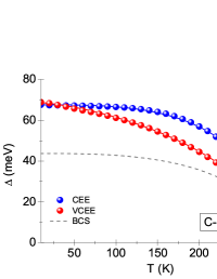
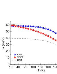
Figure 5: The order parameter as a function of temperature obtained using the classical formalism of Eliashberg equations CEE and Eliashberg equations with the vertex corrections VCEE. The $\mu^{\star}=0.1$ was assumed. Figure (a) the results obtained for the C-S-H system. Figure (b) the results for ${\rm LaH_{10}}$ superconductor. The colored spheres represent numerical results. Solid lines were obtained with Eq. (12). The dashed lines are predictions of BCS theory.

The physical values of order parameter presented in Fig. 5 and Fig. 15 were obtained by using the analytical continuation method ($\Delta_{n}\rightarrow\Delta(\omega)$) Beach et al. (2000). The sample functions $\Delta(\omega)$ and $Z(\omega)$ for C-S-H and LaH₁₀ superconductors taking into account vertex corrections are presented in Fig. 6. The characteristic maxima and minima of discussed functions correspond to frequency regions with the particularly high electron-phonon coupling.

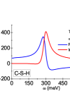
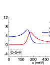
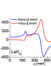
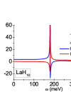
Figure 6: The real and imaginary part of order parameter (a, c), and wave function renormalization factor (b, d) on real axis for $T=T_{0}$. Results obtained for C-S-H and LaH₁₀ superconductors.

III Intermediate values of C-S-H electron-phonon coupling constant

III.1 Electron and phonon properties

The target structure that we selected for our analysis from the paper Snider et al. (2020) was optimized by Kohn-Sham density function theory (DFT) Parr and Yang (1989), within the projector augmented wave (PAW) method and with the generalized gradient approximation of Perdew-Burke-Ernzerhof (GGA-PBE) to the exchange-correlation functional Perdew et al. (1996) as implemented in the Quantum-Espresso ab initio simulation package Giannozzi et al. (2009, 2017).

The kinetic energy cut-off for the wave function is set to $80$ Ry and the kinetic energy cut-off for charge density is $800$ Ry. The Brillouin zone is sampled utilizing a $6\times 6\times 6$ k-mesh in the Monkhorst-Pack scheme to reach the convergence of better than $1$ meV per atom. During the geometric optimization, both lattice constants and atomic positions are fully relaxed by using the Broyden-Fletcher-Goldfarb-Shanno (BFGS) quasi-Newton algorithm Billeter et al. (2003) until the residual forces acting on the atoms remain smaller than $0.001$ eV/Å and the total energy change is smaller than $10^{-5}$ eV. The underlying structure relaxation indicates that the stoichiometry (H₂S)(CH₄)H₂ is a mixture of CH₄, H₂S and hydrogen molecules in the host framework (see inset in Fig. 7 (b)). Moreover, the pressure-dependences optimization shows that the unit-cell volume of carbonaceous sulfur hydride decreases from $121.87$ Å³ at $150$ GPa to $98.61$ Å³ at $275$ GPa.

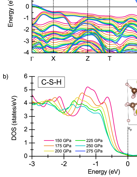
Figure 7: (a) Electron structure; and (b) electron density of states for C-S-H system. The inset shows the crystal structure of carbonaceous sulfur hydride at $267$ GPa.

As shown in Fig. 7, the calculated band structure of carbonaceous sulfur hydride exhibits metallic character above $225$ GPa. As a result, we observe the non-zero value of total density of states (DOS) at the Fermi level. It should be noted, that the obtained results agree with the pressure dependence of $T_{C}$ reported by Snider et al. in paper Snider et al. (2020) where, the sharp increase in $T_{C}$ is observed above $220$ GPa. This can suggest existence of pressure-induced phase transition like in the case of H₃S Drozdov et al. (2015); Mozaffari et al. (2019).

The phonon properties were computed by using the PHONOPY program Togo and Tanaka (2015). The phonon dispersion along $\Gamma$-K-Z-T-V-$\Gamma$ high-symmetry line in the first Brillouin zone is plotted in Fig. 8. No negative phonon branches were found, indicating that the investigated system is dynamically stable in the pressure range from $225$ to $275$ GPa. To know more about the atomic vibration information, the atom-projected phonon DOS curves are also plotted. We find that since the S and C atoms are heavier than the H atom, the vibration modes at the low-energy range are mainly contributed by S and C atoms. The vibration of H atoms contributes to the whole range of energy and is the only contribution to the modes for energy in the range of $\sim$200-370 meV. Interestingly, at higher energy, the phonon modes from C appear again. This result highlights that the H atoms play a dominant role in superconductivity, but C vibrations at high frequencies, are also important because increase the maximal phonon frequency. Which in turn, according to the BCS theory, is one of the reasons responsible for the high critical temperature.

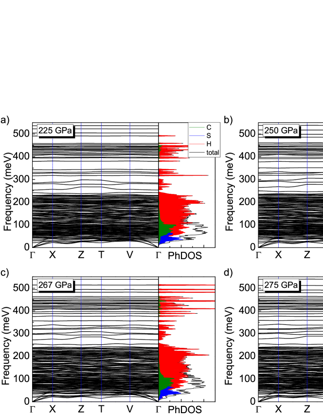
Figure 8: Phonon dispersion curves and phonon density of states (PhDOS) projected onto C, S and H atoms for carbonaceous sulfur hydride at $225$, $250$, $267$, and $275$ GPa.

III.2 Thermodynamic properties of superconducting state at $p\in\{225,250,267,275\}$ GPa

Table 3: Basic thermodynamic parameters characterizing the superconducting state in C-S-H system. Theoretical and experimental results for the pressure of $267$ GPa.

Thermodynamic parameter	CEE model ($\omega_{0}=\omega_{D}$)	CEE model ($\omega_{0}=100$ meV)	VCEE model ($\omega_{0}=100$ meV)	Exp.
$\omega_{D}$ (K)	6258.7	-	-	-
$\mu^{\star}$	0.1	0.1 (0.2)	0.1	-
$\lambda$	0.75	3.26 (3.95)	3.31	-
$T_{C}$ (K)	287.7	287.7 (287.7)	287.7	287.7
$\Delta\left(0\right)$ (meV)	46.05	67.64 (69.28)	68.94	-
$R_{\Delta}$	3.71	5.46 (5.59)	5.56	-
$Z\left(T_{0}\right)$	1.74	3.56 (4.09)	3.48	-
$Z\left(T_{C}\right)$	1.75	4.26 (4.95)	2.69	-
$H_{C}\left(0\right)/\sqrt{\rho\left(\varepsilon_{F}\right)}$ (meV)	210.90	393.97	-	-
$R_{H}$	0.159	0.177	-	-
$\Delta C\left(T_{C}\right)/k_{B}\rho\left(\varepsilon_{F}\right)$ (meV)	524.21	2650.32	-	-
$R_{C}$	1.84	2.37	-	-

Table 4: Basic thermodynamic parameters characterizing the superconducting state in C-S-H system. Theoretical and experimental results for the pressure of $225$ GPa, $250$ GPa, and $275$ GPa. It has been assumed $\omega_{0}=\omega_{D}$.

Parameter	CEE ($225$ GPa)	Exp.	CEE ($250$ GPa)	Exp.	CEE ($275$ GPa)	Exp.
$\omega_{D}$ (K)	6229.5	-	6245.5	-	6264.2	-
$\mu^{\star}$	0.1	-	0.1	-	0.1	-
$\lambda$	0.65	-	0.71	-	0.75	-
$T_{C}$ (K)	200	200	255	255	286	286
$\Delta\left(0\right)$ meV	31.53	-	40.60	-	45.68	-
$R_{\Delta}$	3.72	-	3.68	-	3.93	-
$Z\left(T_{0}\right)$	1.64	-	1.70	-	1.73	-
$Z\left(T_{C}\right)$	1.65	-	1.71	-	1.75	-
$H_{C}\left(0\right)/\sqrt{\rho\left(\varepsilon_{F}\right)}$ meV	144.74	-	186.61	-	212.18	-
$R_{H}$	0.154	-	0.157	-	0.154	-
$\Delta C\left(T_{C}\right)/k_{B}\rho\left(\varepsilon_{F}\right)$ meV	372.48	-	470.15	-	538.99	-
$R_{C}$	1.99	-	1.90	-	1.94	-

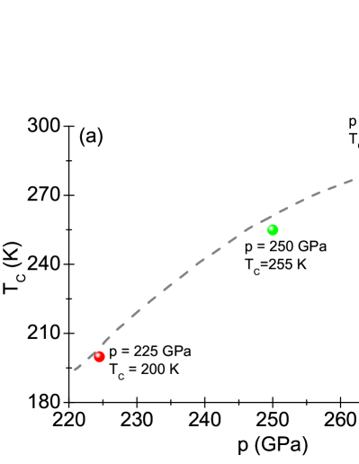
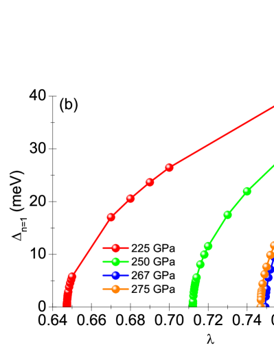
Figure 9: (a) Critical temperature of superconducting state in the C-S-H system for selected values of pressure. The blue, red and green points represent experimental data contained in the paper Snider et al. (2020). The orange point was obtained by using approximation curve (gray dashed line). (b) Maximum value of order parameter as a function of electron-phonon coupling constant. The characteristic frequency $\omega_{0}$ is equal to Debye frequency. The results were obtained in the CEE approach ($\mu^{\star}=0.1$).

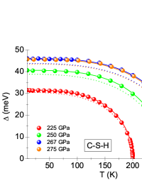
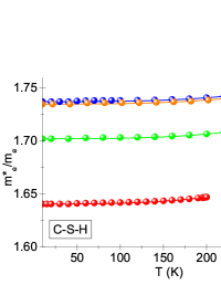
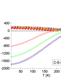
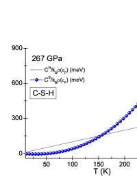
Figure 10: (a) Order parameter $\Delta$ as a function of temperature obtained by using the classical Eliashberg formalism ($\mu^{\star}=0.1$). The numerical results are represented by circles. The solid lines have been obtained using Eq. (12). The dashed lines represent the predictions of BCS theory. (b) Ratio of the electron effective mass to the electron band mass as a function of temperature. The numerical results are represented by circles. The solid lines have been obtained using Eq. (13). (c) Lower panel: the free energy difference between superconducting and normal state as a function of temperature. Upper panel: the influence of temperature on thermodynamic critical field. (d) The specific heat of superconducting and normal state as a function of temperature ($p=267$ GPa).

In the first step, we assumed that characteristic frequency $\omega_{0}$ in the electron-phonon pairing kernel (Eq. (I)) is equal to Debye frequency $\omega_{D}$. The values of $\omega_{D}$ were read from the data obtained by DFT method (see also Tab. 3 and Tab. 4). For the crystal structure considered in the study, the Debye frequencies assume high values of $\sim 6200$ K. This result is caused by existence of the quasi-free hydrogen molecules present in the C-S-H structure, which was illustrated on the phonon density of state graph (Fig. 8) obtained for the pressure values $225$ GPa, $250$ GPa, $267$ GPa, and $275$ GPa.

The basic thermodynamic parameters of superconducting state in C-S-H system were determined within the framework of classic Eliashberg equations (see Appx. I). We solved the Eliashberg equations using the numerical methods that we developed in the paper Szczȩśniak (2006). For $M=2200$ equations, the physically correct solutions can be obtained in temperature range from $T_{0}=10$ K to $T_{C}$. Note that there is the restriction for solutions of Eliashberg equations in the low temperatures due to the fact that temperature zero Kelvin corresponds infinite number of the Matsubara frequencies ($M=+\infty$).

The depairing electron correlations were considered parametrically using the Coulomb pseudopotential $\mu^{\star}$ Morel and Anderson (1962). We assumed in the numerical calculations $\mu^{\star}=0.1$.

The values of electron-phonon coupling constant $\lambda$ were calculated on the basis of experimental critical temperature values (Fig. 9 (a)) by the equation $\left[\Delta_{n=1}\right]_{T=T_{C}}=0$ (see also Fig. 9 (b)). It turns out that for the pressures considered in the study, the electron-phonon coupling constant range from $0.65$ to $0.75$ - the exact results can be found in Tab. 3 and Tab. 4. From the physical point of view, this means that superconducting state in C-S-H system is induced by electron-fonon interaction characterized by the intermediate value of coupling constant. This means that the high value of critical temperature for C-S-H results primarily from the high value of Debye frequency.

In Fig. 10 (a) we have presented the temperature dependence of order parameter for pressure values of $225$ GPa, $250$ GPa, $267$ GPa, and $275$ GPa. The physical values of $\Delta$ have been calculated using the method of analytical continuation characterized in Appx. I. It can be seen that due to relatively low values of electron-phonon coupling constant, the functions of order parameter do not differ substantially from the curves of BCS theory Bardeen et al. (1957a, b). In particular, the CEE numerical results can be parameterized by the formula:

$$\Delta\left(T\right)=\Delta\left(0\right)\sqrt{1-\left(\frac{T}{T_{C}}\right)^{\eta}},$$ (12)

where $\Delta\left(0\right)=\Delta\left(T_{0}\right)$ and $\eta=3.25$. As part of the BCS theory, we get $\eta=3$ and $\Delta\left(0\right)=1.765k_{B}T_{C}$ Eschrig (2001). In the case of numerical results, the ratio of order parameter to critical temperature ranges from $3.7$ to $3.9$ (Tab. 3 and Tab. 4). For the BCS theory, we get the value $3.53$ Bardeen et al. (1957a, b).

The Eliashberg formalism allows to calculate the ratio of electron effective mass ($m^{\star}_{e}$) to electron band mass $m_{e}$. The numerical results obtained with the Eliashberg equations are collected in Fig. 10 (b). They can be parameterized with the formula:

$$m_{e}^{\star}/m_{e}=\left[Z\left(T_{C}\right)-Z\left(T_{0}\right)\right](T/T_{C})^{\eta}+Z\left(T_{0}\right),$$ (13)

where the values of $Z\left(0\right)=Z\left(T_{0}\right)$ and $Z\left(T_{C}\right)=1+\lambda$ can be found in the Tab. 3 or Tab. 4. Note that in the case of BCS theory, we get $m_{e}^{\star}=m_{e}$.

In the next step, we have calculated numerically temperature dependence of free energy difference between the superconducting and the normal state $\Delta F\left(T\right)$, the thermodynamic critical field $H_{C}\left(T\right)$, and the specific heat in superconducting $C^{S}\left(T\right)$ and normal $C^{N}\left(T\right)$ state. The results have been presented in Fig. 10 (c) and (d). The characteristic values of discussed functions have been summarized in Tab. 3 and Tab. 4.

Based on obtained data, the following dimensionless ratios can be calculated: $R_{H}=T_{C}C^{N}\left(T_{C}\right)/H_{C}^{2}\left(0\right)$ and $R_{C}=\Delta C\left(T_{C}\right)/C^{N}\left(T_{C}\right)$. On the basis of Tab. 3 and Tab. 4, we can conclude that their values do not differ substantially from those predicted by BCS theory ($0.168$ and $1.43$) Bardeen et al. (1957a, b).

IV High value of C-S-H electron-phonon coupling constant

IV.1 The thermodynamic properties of C-S-H superconducting state at $p=267$ GPa

The calculations based on use of genetic evolutionary algorithms and DFT method Hu et al. (2020) suggest also the different scenario than proposed for C-S-H system in the paper by Sinder et al. Snider et al. (2020). The authors of article Hu et al. (2020) showed that the replacement of small amount of sulfur atoms by carbon in compounds like ${\rm C_{1}S_{15}H_{48}}$ and ${\rm C_{1}S_{17}H_{54}}$ results in stronger electron-phonon coupling and higher averaged phonon frequency that increases with the pressure. As a result, the critical temperature reaches the room temperature value at $\sim 270$ GPa. Additionally, the calculated superconducting transition temperature of ${\rm C_{1}S_{15}H_{48}}$ and ${\rm C_{1}S_{17}H_{54}}$ as a function of pressure shows the good agreement with experimental measurements for C-S-H Snider et al. (2020).

Under the approach that we consider in this paper, for the pressure of $267$ GPa, the Hu et al. results Hu et al. (2020) can be reproduced by taking $\omega_{0}\sim 100$ meV. Using the experimental data obtained for critical temperature (Fig. 9 (a)) and equation $[\Delta_{n=1}]_{T=T_{C}}=0$, the calculated values of electron-phonon coupling constant in CEE model are $3.26$ and $3.95$ for $\mu^{\star}=0.1$ and $\mu^{\star}=0.2$, respectively. In paper Hu et al. (2020) estimated value of $\lambda$ for ${\rm C_{1}S_{17}H_{54}}$ is approximately $2.8$. The above-mentioned results clearly suggest that the high value of critical temperature in C-S-H system is induced by high value of the electron-phonon coupling constant and high value of the logarithmic phonon frequency $\omega_{\rm ln}$ of about $1550$ K (the value of Debye frequency is about $3597$ K Hu et al. (2020)).

Taking into account the present case, in the area of strong electron-phonon coupling, the importance of vertex corrections for the electron-phonon interaction should be additionally examined. Our remark is due to the fact that their influence on obtained results is related to the value of dimensionless ratio $\lambda\omega_{D}/\varepsilon_{F}$, which explicitly depends on the value of electron-phonon coupling constant Pietronero and Strässler (1992); Pietronero et al. (1995); Grimaldi et al. (1995). For C-S-H system its value is equal to $0.02$, which means that in the static limit vertex corrections do not significantly modify the results obtained under the classical Eliashberg formalism. Nevertheless, when one considers the full dependence of order parameter on Matsubara frequency (dynamic effects) then the answer to question about the significance of vertex corrections requires the self-consistent solution of appropriately modified Eliashberg equations Freericks et al. (1997) (see VCEE schema discussed in detail in Appx. II). Our calculations showed that in VCEE scheme, for the Coulomb pseudopotential $0.1$, the value of electron-phonon coupling constant is slightly increased ($\lambda=3.31$) compared to the result obtained under CEE scheme ($\lambda=3.26$). The full order parameter dependencies on $\lambda$ for both CEE and VCEE schemas are shown in Fig. 11.

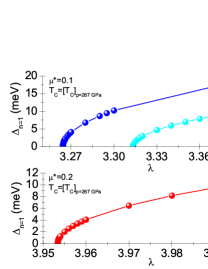
Figure 11: Maximum value of order parameter as a function of electron-phonon coupling constant for the characteristic frequency of $100$ meV. Assumed $T=[T_{C}]_{p=267\hskip 2.84526pt{\rm GPa}}$ and $\mu^{\star}\in\{0.1,0.2\}$. The results were obtained under CEE and VCEE model.

In Fig. 5 (a) we plotted the temperature dependence of order parameter determined using the classical Eliashberg equations and equations with vertex corrections. We obtained the physical values of order parameter using the method of analytical continuation the solutions of Eliashberg equations from imaginary axis Beach et al. (2000) (see also Appx. I and Appx. II). It can be seen that due to significant strong-coupling effects, the obtained curves differ very clearly from BCS curve Bardeen et al. (1957a, b). In particular, the numerical results can be parameterized using the formula Eq. (12). In the CEE approach we get $\eta=3.35$, while for VCEE the exponent $\eta$ is equal to $1.5$. Fig. 5 (a) allows to evaluate the impact of vertex corrections on the values of order parameter. In particular, it can be seen that vertex corrections clearly underestimate the $\Delta\left(T\right)$ values in temperature range from about $50$ K to about $275$ K. Outside the indicated range, their importance is negligible, which means that near zero Kelvin or near $T_{C}$, the thermodynamic properties of C-S-H system, with high accuracy, can be calculated within classical Eliashberg formalism. Note that in the case of ${\rm LaH_{10}}$ superconductor ($p=190$ GPa and $T_{C}=260$ K Somayazulu et al. (2019)), the very similar scenario as for C-S-H is realized, as presented in Fig. 5 (b). The method for obtaining results for ${\rm LaH_{10}}$ was discussed in Appx. VI. The $\eta$ exponent values are $3.4$ and $1.5$ for the CEE and VCEE formalism, respectively.

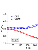
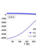
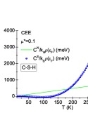
Figure 12: (a) The ratio of effective mass to band mass of electron as a function of temperature. The solid line was obtained with Eq. (13). (b) Upper panel: the thermodynamic critical field as a function of temperature. Lower panel: the free energy difference between superconducting and normal states as a function of temperature. (c) The specific heat of superconducting and normal states as a function of temperature.

In Fig. 12 (a), we plotted the temperature dependence of ratio: $m^{\star}_{e}/m_{e}$ - the effective mass of electron to the band mass of electron. Due to the very high value of electron-phonon coupling constant, also the ratio $m^{\star}_{e}/m_{e}$ takes high values. In particular, under classical Migdal-Eliashberg scheme, we obtained $m^{\star}_{e}/m_{e}=3.56$ ($T=T_{0}$). On the other hand, for $T=T_{C}$, the value of $m^{\star}_{e}/m_{e}$ is equal to $4.26$. This result is consistent with exact analytical result: $m^{\star}_{e}/m_{e}=1+\lambda$ Carbotte (1990), which confirms the high quality of presented numerical results.

The results collected in Fig. 12 (a) prove also that the vertex corrections clearly change the temperature dependence of effective mass of the electron. Importantly, with the increasing temperature, the ratio $m^{\star}_{e}/m_{e}$ significantly decreases reaching the value of $2.69$ for critical temperature.

As we have shown in area of the low temperatures ($T\sim T_{0}$) and in vicinity of the critical temperature, the vertex corrections slightly affect the values of order parameter. This means that in the temperature ranges of interest, the thermodynamic parameters of superconducting state can be calculated within the CEE scheme. All the formulas needed for this purpose have been collected and discussed in Appx. I.

In Fig. 12 (b) we presented the influence of temperature on the value of free energy difference between superconducting and normal states ($\Delta F$). From this, the temperature dependence of thermodynamic critical field $H_{C}$ can be determined. For $T=T_{0}$ the value of thermodynamic critical field is equal to $H_{C}\left(0\right)/\sqrt{\rho\left(\varepsilon_{F}\right)}=393.97$ meV (see also Tab. 3). This means that the dimensionless ratio $R_{H}$ is equal to $0.177$. Recall that for all superconducting systems, the BCS model predicts $R_{H}=0.168$ Bardeen et al. (1957a, b).

The forms of specific heat curves for superconducting and normal states are plotted in Fig. 12 (c). The specific heat jump occurring at critical temperature is characterized by the value $\Delta C\left(T_{C}\right)/k_{B}\rho\left(\varepsilon_{F}\right)=2650.32$ meV. Hence, the dimensionless ratio $R_{C}$ is equal to $2.37$. The BCS model predicts $R_{C}=1.43$ Bardeen et al. (1957a, b).

V Characterization of selected hydrogen-rich compounds in terms of superconducting state

The literature that describing the superconducting state in hydrogen-rich compounds is very extensive (see Szczȩśniak and Durajski (2013); Durajski et al. (2020) and references therein). In Tab. 5, we have collected the most important information on experimental and theoretical results obtained so far. In particular, we have taken into account superconductors containing carbon and sulphur due to the fact that these elements are present in C-S-H system. Additionally, we have reported results for $\rm{LaH_{10}}$, $\rm{YH_{10}}$, and $\rm{YH_{6}}$, due to the very high value of critical temperature in these compounds.

Note that research on sulphur in the context of superconductivity dates back to $1997$, when Struzhkin et al. Struzhkin et al. (1997) experimentally demonstrated the disappearance of electrical resistance in temperature range from $10$ K to $17$ K, and the pressure of $93$-$157$ GPa. Thus, they established the record value of critical temperature for pure element, for that moment. Subsequently, the theoretical analysis carried out in $2014$ by Li et al. Li et al. (2014) suggested the existence of superconducting state with much higher value of critical temperature ($T_{C}=80$ K) in $\rm{H_{2}S}$ for the pressure $160$ GPa. The experimental verification of Li et al. Li et al. (2014) result by Drozdov et al. Drozdov et al. (2015) unexpectedly showed that the value of critical temperature was almost twice as high ($T_{C}=$150 K).

In addition, in the same experiment Drozdov et al. (2015), the superconducting properties of $\rm{H_{3}S}$ were investigated, confirming the previous theoretical predictions of Duan et al. Duan et al. (2014) about superconducting state with the record critical temperature (at that time) of as much as $203$ K. Referring to the Tab. 5, we can see that the superconducting properties of sulfur and hydrogen compounds have been tested for the wide pressure range, however, no higher critical temperature value than $T_{C}=203$ K has been found. While extending the research, promising results were obtained by adding carbon to sulfur and hydrogen. For example, the theoretically analyzed $\rm{CSH_{7}}$ compound can presumably become superconducting at temperature of about $200$ K Cui et al. (2020). On the other hand, the C-S-H system, widely discussed in this paper, seems to be the undisputed record holder, which according to the experimental data reaches the $T_{C}$ value of $287.7$ K Snider et al. (2020).

The $\rm{YH_{6}}$, $\rm{LaH_{10}}$, and $\rm{YH_{10}}$ compounds were indicated as potential high-temperature superconductors based on the results of theoretical considerations ($\rm{YH_{6}}$ in 2015 Li et al. (2015), $\rm{LaH_{10}}$ and $\rm{YH_{10}}$ two years later Liu et al. (2017)). Although, according to calculations, $\rm{YH_{10}}$ compound has the highest critical temperature among mentioned superconductors (see Tab. 5), this result has not been confirmed experimentally so far. The situation is different for the $\rm{LaH_{10}}$ compound, for which in $2019$ it was experimentally demonstrated that its critical temperature value is equal to $260$ K ($p=190$ GPa) Somayazulu et al. (2019). This result agrees quite well with previous theoretical predictions Liu et al. (2017). For $\rm{YH_{6}}$ compound, the latest experimental studies Troyan et al. (2021) show that theoretical calculations have overestimated the critical temperature (by about $40$ K) Li et al. (2015). In our opinion, this inconsistency is seeming. The detailed analysis of this issue is provided in Appx. VII.

It should be noted that all of mentined hydrogen-rich compounds for which $T_{C}$ exceeds $200$ K are characterized by the high value of electron-phonon coupling constant (see Tab. 5), what suggests the similar scenario for C-S-H system.

Table 5: Selected elements or compounds containing hydrogen in which the superconducting state has been confirmed or is expected to exist.

Stoichiometry	$p$ (GPa)	Structure	$\lambda$	$\omega_{{\rm ln}}/k_{B}$ (K)	$\mu^{\star}$	$T^{\rm CEE}_{C}$ (K)	$T^{\rm Exp.}_{C}$ (K)	Theor./Exp.
${\rm CSH_{7}}$	100	Cm	1.20	1091	0.1	108	-	Theor. Cui et al. (2020)
${\rm CSH_{7}}$	150	R3m	2.47	925	0.1	194	-	Theor. Cui et al. (2020)
${\rm CSH_{7}}$	200	R3m	1.35	1379	0.1	158	-	Theor. Cui et al. (2020)
${\rm CSH_{7}}$	150	Pmna	3.06	672	0.1	170	-	Theor. Cui et al. (2020)
${\rm CSH_{7}}$	200	Pmna	1.06	1622	0.1	138	-	Theor. Cui et al. (2020)
C-S-H	225	-	-	-	-	-	200	Exp. Snider et al. (2020)
C-S-H	250	-	-	-	-	-	255	Exp. Snider et al. (2020)
C-S-H	267	-	-	-	-	-	287.7	Exp. Snider et al. (2020)
C-S-H	275	-	-	-	-	-	286	Exp. Snider et al. (2020)
$\rm H_{2}S$	160	$P1\rightarrow Cmca$	$\sim 1.2$	$\sim 1000$	0.13	82	-	Theor. Li et al. (2014)
$\rm H_{2}S$	150	-	-	-	-	-	150	Exp. Drozdov et al. (2015)
$\rm H_{2}S$	130-180	$P1,Cmca$	1.28	960	0.15	31-88	-	Theor. Durajski et al. (2015)
$\rm H_{3}S$	200	Im$\overline{3}$m	2.19	1335	0.1	204	-	Theor. Duan et al. (2014)
$\rm H_{3}S$	157	Im$\overline{3}$m	1.94	1321	0.16	216	-	Theor. Errea et al. (2016)
$\rm H_{3}S$	155	-	-	-	-	-	203	Exp.Drozdov et al. (2015)
$\rm H_{3}S$	150	$R3m$	2.067	1056	0.123	203	-	Theor. Durajski et al. (2016)
$\rm H_{3}S$	250	Im$\overline{3}$m	1.31	1485	0.13	164	-	Theor. Durajski and Szczȩśniak (2017)
$\rm H_{3}S$	350	Im$\overline{3}$m	1.22	1301	0.13	129	-	Theor. Durajski and Szczȩśniak (2017)
$\rm H_{3}S$	450	Im$\overline{3}$m	1.26	1464	0.13	146	-	Theor. Durajski and Szczȩśniak (2017)
$\rm H_{3}S$	500	Im$\overline{3}$m	1.32	1454	0.13	156	-	Theor. Durajski and Szczȩśniak (2017)
$\rm LaH_{10}$	300	$Fm\overline{3}m$	1.78	1488	0.1 (0.13)	254 (241)	-	Theor. Liu et al. (2017)
$\rm LaH_{10}$	250	sodalite-like fcc	2.2	1253	0.1 (0.13)	274 (257)	-	Theor. Liu et al. (2017)
$\rm LaH_{10}$	190	-	-	-	-	-	260	Exp. Somayazulu et al. (2019)
$\rm LaH_{10}$	170	-	-	-	-	-	250	Exp. Drozdov et al. (2019)
$\rm LaH_{10}$	150	R$\overline{3}$m	2.2	-	0.1	215	-	Theor. Kostrzewa et al. (2020)
$\rm LaH_{10}$	190	Fm$\overline{3}$m	2.8	-	0.1	260	-	Theor. Kostrzewa et al. (2020)
$\rm LaH_{10}$	170	$Fm\overline{3}m$	3.94	801	0.2	259	-	Theor. Kruglov et al. (2020)
$\rm LaH_{10}$	150	$R\overline{3}m$	2.77	833	0.2	203	-	Theor. Kruglov et al. (2020)
$\rm YH_{10}$	250	Fm$\overline{3}$m	2.56	1282	0.1 (0.13)	326 (305)	-	Theor.Liu et al. (2017)
$\rm YH_{10}$	300	Im$\overline{3}$m	2.06	1511	0.1 (0.13)	308 (286)	-	Theor.Liu et al. (2017)
$\rm YH_{10}$	250	sodalite-like fcc	2.67	1102	0.1	291	-	Theor.Tanaka et al. (2017)
$\rm YH_{10}$	300	sodalite-like fcc	2.00	1450	0.1	275	-	Theor.Tanaka et al. (2017)
$\rm YH_{6}$	120	Im$\overline{3}$m	2.93	1080	0.1 (0.13)	264 (251)	-	Theor.Li et al. (2015)
$\rm YH_{6}$	166	Im$\overline{3}$m	-	-	-	-	224	Exp. Troyan et al. (2021)
$\rm YH_{6}$	165	Im$\overline{3}$m	1.71	1333	0.1 (0.15)	247 (236)	-	Theor.Troyan et al. (2021)
$\rm YH_{6}$	300	Im$\overline{3}$m	1.73	1612	0.11	290	-	Theor.Heil et al. (2019)
S	93-157	-	-	-	-	-	10-17	Exp.Struzhkin et al. (1997)
S	160	$\beta$-Po	0.75	437	0.127	17	-	Theor.Durajski et al. (2012)
H	480	$I4_{1}/amd$	2.17	1870	0.1 (0.13)	284 (266)	-	Theor. Yan et al. (2011)
H	539	$I4_{1}/amd$	2.01	2016	0.1 (0.13)	291 (272)	-	Theor.Yan et al. (2011)
H	608	$I4_{1}/amd$	1.89	2106	0.1 (0.13)	291 (270)	-	Theor.Yan et al. (2011)
H	802	$I4_{1}/amd$	1.68	2239	0.1 (0.13)	282 (260)	-	Theor.Yan et al. (2011)
H	802	$I4_{1}/amd$	1.7	-	0.1 (0.2)	332.7 (259.4)	-	Theor.Durajski et al. (2014)
H	2000	fcc	7.32	1035	0.1 (0.5)	631 (413)	-	Theor.Szczȩśniak and Jarosik (2009)
$\rm H_{2}$	494	2D model	0.628	7955.064	0.17385	84.49	-	Theor. Kostrzewa et al. (2021)
$\rm H_{2}$	686	2D model	0.573	10985.66	0.17997	64.66	-	Theor. Kostrzewa et al. (2021)

VI Detailed characteristics of superconducting state in ${\rm LaH_{10}}$ compound

For LaH₁₀ the calculations of atomic structure relaxation, electronic structure, and phonon properties were performed based on the DFT method within the generalized gradient approximation of the Perdew-Burke-Ernzerhof exchange-correlation functional. The Brillouin zone was sampled using a $24\times 24\times 24$ k-points grid according to the Monkhorst-Pack scheme. On the base of convergence tests, the kinetic energy cut-off for the wave functions and charge density were taken as $80$ Ry and $1000$ Ry, respectively. The cubic clathrate-type structure of investigated system with the space group Fm$\overline{3}$m consists of the cage of $32$ H atoms surrounding a La atom. The optimized lattice parameters $a=b=c$ of LaH₁₀ at $150$ GPa and $190$ GPa are $5.0964$ and $4.9834$ Å, repectively. We found that LaH₁₀ has a DOS that reaches $0.91-0.93$ states/eV at the Fermi level, because of the presence of a van Hove singularity in the vicinity, as shown in Fig. 13. By increasing the pressure, the DOS peak can be modulated.

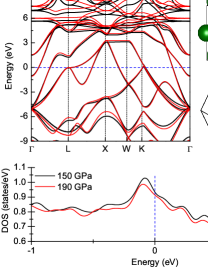
Figure 13: Band structures along the $\Gamma$-L-X-W-K-$\Gamma$ high-symmetry line and DOS of LaH₁₀ at $150$ GPa (black lines) and $190$ GPa (red lines) with their Fermi energies set to be zero. Moreover, the optimized crystal structure and the Brillouin zone for cubic (Fm$\overline{3}$m) clathrate-type structure with special k-point paths were plotted.

Thermodynamic parameters of the ${\rm LaH_{10}}$ superconductor, subjected to external pressure of $190$ GPa, were determined taking into account the Eliashberg equations on imaginary axis (see Appx. I and Appx. II). In the first step, we calculated the value of electron-phonon coupling constant. We used the condition: $\left[\Delta_{n=1}\right]_{T=T_{C}}=0$, where $T_{C}=260$ K is experimental result taken from the paper Somayazulu et al. (2019). For classical Eliashberg equations, we obtained: $\lambda=2.82$, for Eliashberg equations taking into account the vertex corrections, we had: $\lambda=2.77$. Based on discussed data, we conclude that the ${\rm LaH_{10}}$ superconductor is the system characterized by strong electron-phonon coupling. By taking vertex corrections into account - the value of $\lambda$ can be decreased by $1.3\%$.

Fitting the value of electron-phonon coupling constant to experimental results is presented in Fig. 14 (a). In particular, we assumed: $\mu^{\star}=0.1$, $\omega_{0}=100$ meV, and $\omega_{C}=1$ eV. We have obtained the stable solutions of Eliashberg equations for $T\geq T_{0}=15$ K.

The full dependence of order parameter on temperature we plotted in Fig. 5 (b). In turn the influence of temperature on the value of effective electron mass to band electron mass ratio is presented in Fig. 14 (b). It can be seen that, analogically to C-S-H system (see Fig. 12 (a)), the vertex corrections to electron-phonon interaction noticeably lower the value of effective mass of electron.

The dimensionless ratio $R_{\Delta}$ for the ${\rm LaH_{10}}$ superconductor is equal $5.25$ and $5.33$, respectively for schema CEE and VCEE. These results are due to significant retardation and strong-coupling effects. The other thermodynamic parameters of superconductor ${\rm LaH_{10}}$ have already been analyzed by us in CEE scheme and described in detail in the publication Kostrzewa et al. (2020).

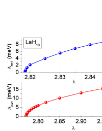
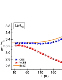
Figure 14: (a) The dependence of maximum value of order parameter on the electron-phonon coupling constant ($T=T_{C}$). (b) The influence of temperature on the effective electron mass. Spheres represent the numerical results. The orange line was obtained using the analytical formula Eq. (13).

VII The thermodynamic parameters of superconducting state for ${\rm YH_{6}}$ compound

The superconducting properties of ${\rm YH_{6}}$ compound attracted the attention of researchers several years ago. Calculations carried out in 2014 by Li et al. suggested the high transition teperature value of $251$ K-$264$ K at $120$ GPa Li et al. (2015). Additionally, in 2019 it was suggested that the value of $\rm{T_{C}}$ at $300$ GPa could be as high as $290$ K Heil et al. (2019). In contrast, experiments conducted in 2020 showed that the critical temperature value is equal to $224$ K at $166$ GPa ($Im\bar{3}m$ structure) Troyan et al. (2021), so is lower than theoretically predicted value of ${T_{C}}$.

Table 6: The input parameters to Eliashberg equations for ${\rm YH_{6}}$ compound.

$p$	$166$ GPa
$T_{C}$ Troyan et al. (2021)	$224$ K
$\omega_{D}$ (anharmonic) from $\alpha^{2}F(\omega)$ for $Im\bar{3}m$ Troyan et al. (2021)	$210.24$ meV
$\lambda$ Troyan et al. (2021)	$1.71$
$\Omega_{C1}$	3$\omega_{D}$
$\mu^{\star}_{1}$	$0.277$
$\Omega_{C2}$	10$\omega_{D}$
$\mu^{\star}_{2}$	$0.363$
The Migdal ratio: $\frac{\omega_{D}}{\varepsilon_{F}}$	$0.013$
$\lambda\frac{\omega_{D}}{\varepsilon_{F}}$	$0.023$

In the first step, we performed the numerical calculations for ${\rm YH_{6}}$ within classical Eliashberg formalism (CEE). We used the anharmonic Eliashberg function determined in the paper Troyan et al. (2021) (see also Tab. 6). For the standard value of Coulomb pseudopotential $\mu^{\star}=0.1$ (the pink spheres in Fig. 15 (a)), we obtained slightly higher critical temperature value ($T_{C}=236.8$ K) than in the experiment ($T_{C}=224$ K). In the next step, we calculated the exact value of Coulomb pseudopotential for CEE scheme based on the equation $\left[\Delta_{n=1}\left(\mu^{\star}\right)\right]_{T=T_{C}}=0$, assuming that $\Omega_{C}=3\omega_{D}$ (the dark cyan spheres in Fig. 15 (b)). The obtained result is as follows: $\mu^{\star}=0.123$. Then, we determined the temperature dependence of order parameter (the dark cyan spheres in Fig. 15 (a)). It can be easily noticed that the obtained results allow to determine the width of superconducting gap, which in the analyzed case is: $2\Delta(T_{0})=86.28$ meV. On this basis, we have obtained: $R_{\Delta}=4.45$.

Note that in the publication Troyan et al. (2021), the numerical calculations were also performed using the Eliashberg formalism (although the different form of Eliashberg equations was used). In the harmonic case, they received $T_{C}=251$ K for $\mu^{\star}=0.195$ and $T_{C}=261$ K-$272$ K for $\mu^{\star}=0.15-0.1$. In the anharmonic case, the results are: $T_{C}=226$ K for $\mu^{\star}=0.195$ and $T_{C}=236$ K-$247$ K for $\mu^{\star}=0.15-0.1$. As can easily be seen, the best outcomes (most close to experimental result) are given by the results obtained for anharmonic $\alpha^{2}F(\omega)$ of $Im\bar{3}m$-${\rm YH_{6}}$ ($165$ GPa). However, it can be seen that the relatively high value of Coulomb pseudopotential was used.

For ${\rm YH_{6}}$ we also performed the analysis within VCEE formalism. The input data for Eliashberg equations are collected in Tab. 6. We obtained even higher value of Coulomb pseudopotential ($\mu^{\star}_{1}=0.277$), than Troyan et al. (we have chosen the standard cut-off frequency: $\Omega_{C1}=3\omega_{D}$). Note that the even higher cut-off frequency ($\Omega_{C2}=10\omega_{D}$) leads to even greater undesirable increase in the Coulomb pseudopotential: $\mu^{\star}_{2}=0.363$. The dependence courses of $\Delta_{n=1}$ on $\mu^{\star}$, characterizing the situation discussed by us, are collected in Fig. 15 (b). In Fig. 15 (a), we have plotted the temperature dependencies of order parameter. The results obtained for formalism including vertex corrections, for both calculated values of the Coulomb pseudopotential, converge the entire analyzed temperature range up to $T_{C}=224$ K. It can also be seen that the influence of vertex corrections on the values of order parameter is analogous to ${\rm LaH_{10}}$ superconductor and C-S-H system (strong-coupling case - see Fig. 5).

In area of very low temperatures and temperatures close to the critical temperature the values of order parameter obtained in CEE and VCEE schemes are physically indistinguishable. This result implies that the thermodynamics of superconducting state near temperature $T_{0}$ and close to critical temperature can be analyzed by using the classical Eliashberg approach. The Fig. 16 shows the difference of free energy $\Delta F$, the function of thermodynamic critical field $H_{C}$ and the specific heat in superconducting $C^{S}$ and normal $C^{N}$ states. Negative values of free energy difference indicate the thermodynamic stability of superconducting phase up to critical temperature. Additionally, we can observe a characteristic jump of specific heat occurring in $T_{C}=224$ K, its value equals $544.59$ meV. For ${\rm YH_{6}}$ superconductor, the values of characteristic dimensionless parameters $R_{H}$ and $R_{C}$ are $0.136$ and $1.53$, respectively.

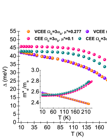
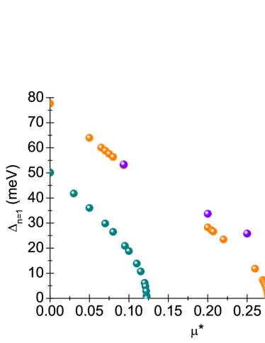
Figure 15: (a) The dependence of order parameter on temperature for ${\rm YH_{6}}$ compound. In the inset, we presented the values of electron effective mass. (b) The dependence of maximum value of the order parameter on Coulomb pseudopotential for $T=T_{C}$.

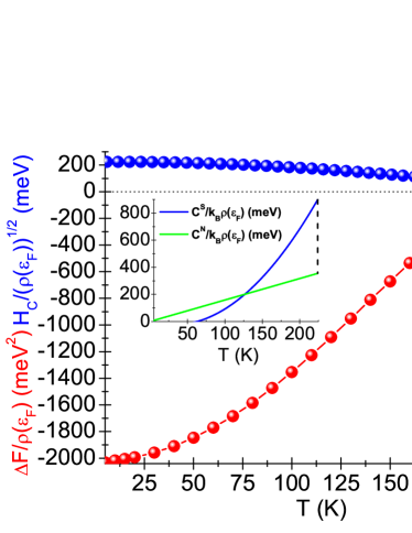
Figure 16: (Lower panel) The free energy difference between superconducting and normal states as a function of temperature. (Upper panel) The thermodynamic critical field as a function of temperature. The inset shows the temperature dependence of specific heat for superconducting and normal state.

VIII Influence of many-body corrections on the order parameter (classical Eliashberg equations)

The classical Eliashberg equations were derived in self-consistent way, in the second order of electron-phonon coupling function ($g^{2}$). This procedure ignores the higher-order many-body corrections that affect the order parameter Carbotte (1990).

Figure 17: The classic (green) and modified (blue) scheme for deriving the Eliashberg equations. The white blocks are common to both methods.

We present the derivation of Eliashberg equations for the higher-order many-body terms in the channel of order parameter. The self-consistent scheme has been characterized by Fig. 17. In particular, the Matsubara Green function is given by formula Fetter and Walecka (1971); Elk and Gasser (1979):

$$\left<\left<\Psi_{\mbox{{\scriptsize{\bf k}}}-\mbox{{\scriptsize{\bf q}}}}|\Psi^{\dagger}_{\mbox{{\scriptsize{\bf k}}}+\mbox{{\scriptsize{\bf q}}}^{\prime}}\right>\right>_{i\omega_{n}}=\left(\begin{array}[]{cc}\left<\left<c_{\mbox{{\scriptsize{\bf k}}}-\mbox{{\scriptsize{\bf q}}}\uparrow}|c^{\dagger}_{\mbox{{\scriptsize{\bf k}}}+\mbox{{\scriptsize{\bf q}}}^{\prime}\uparrow}\right>\right>_{i\omega_{n}}&\left<\left<c_{\mbox{{\scriptsize{\bf k}}}-\mbox{{\scriptsize{\bf q}}}\uparrow}|c_{-\mbox{{\scriptsize{\bf k}}}-\mbox{{\scriptsize{\bf q}}}^{\prime}\downarrow}\right>\right>_{i\omega_{n}}\\ \left<\left<c^{\dagger}_{-\mbox{{\scriptsize{\bf k}}}+\mbox{{\scriptsize{\bf q}}}\downarrow}|c^{\dagger}_{\mbox{{\scriptsize{\bf k}}}+\mbox{{\scriptsize{\bf q}}}^{\prime}\uparrow}\right>\right>_{i\omega_{n}}&\left<\left<c^{\dagger}_{-\mbox{{\scriptsize{\bf k}}}+\mbox{{\scriptsize{\bf q}}}\downarrow}|c_{-\mbox{{\scriptsize{\bf k}}}-\mbox{{\scriptsize{\bf q}}}^{\prime}\downarrow}\right>\right>_{i\omega_{n}}\end{array}\right)\equiv\left(\begin{array}[]{cc}g^{A}_{\mbox{{\scriptsize{\bf k}}}-\mbox{{\scriptsize{\bf q}}}}(i\omega_{n})&g^{B}_{\mbox{{\scriptsize{\bf k}}}-\mbox{{\scriptsize{\bf q}}}}(i\omega_{n})\\ g^{C}_{\mbox{{\scriptsize{\bf k}}}-\mbox{{\scriptsize{\bf q}}}}(i\omega_{n})&g^{D}_{\mbox{{\scriptsize{\bf k}}}-\mbox{{\scriptsize{\bf q}}}}(i\omega_{n})\end{array}\right),$$ (14)

where the symbol $c^{{\dagger}}_{\mbox{{\scriptsize{\bf k}}}\sigma}$ ($c_{\mbox{{\scriptsize{\bf k}}}\sigma}$) represents the electron creation (anihilation) operator with momentum ${\bf k}$ and spin $\sigma\in\{\uparrow,\downarrow\}$. Including the many-body contributions of fourth order of $g$, one can obtain:

$$\left<\left<\psi_{\mbox{{\scriptsize{\bf k}}}-\mbox{{\scriptsize{\bf q}}}}|\psi^{\dagger}_{\mbox{{\scriptsize{\bf k}}}+\mbox{{\scriptsize{\bf q}}}^{\prime}}\right>\right>_{i\omega_{n}}=\left(\begin{array}[]{cc}f^{(1)}_{\mbox{{\scriptsize{\bf k}}}\mbox{{\scriptsize{\bf q}}}}(i\omega_{n})+\omega^{2}_{\mbox{{\scriptsize{\bf q}}}}\cdot g^{A}_{\mbox{{\scriptsize{\bf k}}}-\mbox{{\scriptsize{\bf q}}}}(i\omega_{n})&-(\omega_{n}-\omega_{m})^{2}\cdot g^{B}_{\mbox{{\scriptsize{\bf k}}}-\mbox{{\scriptsize{\bf q}}}}(i\omega_{n})\\ -(\omega_{n}-\omega_{m})^{2}\cdot g^{C}_{\mbox{{\scriptsize{\bf k}}}-\mbox{{\scriptsize{\bf q}}}}(i\omega_{n})&f^{(2)}_{\mbox{{\scriptsize{\bf k}}}\mbox{{\scriptsize{\bf q}}}}(i\omega_{n})+\omega^{2}_{\mbox{{\scriptsize{\bf q}}}}\cdot g^{D}_{\mbox{{\scriptsize{\bf k}}}-\mbox{{\scriptsize{\bf q}}}}(i\omega_{n})\end{array}\right).$$ (15)

The functions appearing in above matrix possesses the following form:

$$f^{(1)}_{\mbox{{\scriptsize{\bf k}}}\mbox{{\scriptsize{\bf q}}}}(i\omega_{n})=\left[g^{-}_{0\mbox{{\scriptsize{\bf k}}}-\mbox{{\scriptsize{\bf q}}}}(i\omega_{n})\right]^{-1}\left(1+n^{ph}_{\mbox{{\scriptsize{\bf q}}}}+n^{ph}_{-\mbox{{\scriptsize{\bf q}}}}\right)+\omega_{\mbox{{\scriptsize{\bf q}}}}\left(1+n^{ph}_{\mbox{{\scriptsize{\bf q}}}}-n^{ph}_{-\mbox{{\scriptsize{\bf q}}}}\right)-2\omega_{\mbox{{\scriptsize{\bf q}}}}n^{e}_{\mbox{{\scriptsize{\bf k}}}-\mbox{{\scriptsize{\bf q}}}\uparrow},$$ (16)

$$f^{(2)}_{\mbox{{\scriptsize{\bf k}}}\mbox{{\scriptsize{\bf q}}}}(i\omega_{n})=\left[g^{+}_{0\mbox{{\scriptsize{\bf k}}}-\mbox{{\scriptsize{\bf q}}}}(i\omega_{n})\right]^{-1}\left(1+n^{ph}_{\mbox{{\scriptsize{\bf q}}}}+n^{ph}_{-\mbox{{\scriptsize{\bf q}}}}\right)+\omega_{\mbox{{\scriptsize{\bf q}}}}\left(1+n^{ph}_{\mbox{{\scriptsize{\bf q}}}}-n^{ph}_{-\mbox{{\scriptsize{\bf q}}}}\right)-2\omega_{\mbox{{\scriptsize{\bf q}}}}(1-n^{e}_{-\mbox{{\scriptsize{\bf k}}}+\mbox{{\scriptsize{\bf q}}}\downarrow}),$$

where: $g^{\pm}_{0\mbox{{\scriptsize{\bf k}}}}(i\omega_{n})=\left[\varepsilon_{\mbox{{\scriptsize{\bf k}}}}\pm i\omega_{n}\right]^{-1}$, are bare electron Green functions that ignore the electron-phonon interaction. Additionally, $\varepsilon_{\mbox{{\scriptsize{\bf k}}}}$ is the electron band energy, and $\omega_{\mbox{{\scriptsize{\bf q}}}}$ represents the phonon dispersion relation. The symbols $n^{e}_{\mbox{{\scriptsize{\bf k}}}\sigma}$ and $n^{ph}_{\mbox{{\scriptsize{\bf q}}}}$ refer to the Fermi-Dirac and the Bose-Einstein functions, respectively. The self-consistent procedure allows to obtain the modified equation for order parameter:

$$\varphi_{\bf k}\left(i\omega_{n}\right)=\frac{k_{B}T}{N}\sum_{m{\bf q}}K^{\left(a\right)}_{\bf kq}\left(\omega_{n}-\omega_{m}\right)K_{\bf q}\left(\omega_{n}-\omega_{m}\right)\frac{\varphi_{{\bf k}-{\bf q}}\left(i\omega_{m}\right)}{D_{{\bf k}-{\bf q}}\left(i\omega_{m}\right)}.$$ (17)

The additional many-body term can be written as:

$$K^{\left(a\right)}_{\mbox{{\scriptsize{\bf k}}}\mbox{{\scriptsize{\bf q}}}}\left(\omega_{n}-\omega_{m}\right)=\frac{\left(\omega_{n}-\omega_{m}\right)^{2}}{\omega^{2}_{n}+\varepsilon^{2}_{\mbox{{\scriptsize{\bf k}}}-\mbox{{\scriptsize{\bf q}}}}}.$$ (18)

Assuming $K^{\left(a\right)}_{\mbox{{\scriptsize{\bf k}}}\mbox{{\scriptsize{\bf q}}}}\left(\omega_{n}-\omega_{m}\right)\rightarrow 1$, we get classic equation for the order parameter. We introduced also the designation: $D_{\mbox{{\scriptsize{\bf k}}}-\mbox{{\scriptsize{\bf q}}}}\left(i\omega_{m}\right)=\left(\omega_{m}Z_{\mbox{{\scriptsize{\bf k}}}-\mbox{{\scriptsize{\bf q}}}}\left(i\omega_{m}\right)\right)^{2}+\varepsilon^{2}_{\mbox{{\scriptsize{\bf k}}}-\mbox{{\scriptsize{\bf q}}}}+\varphi^{2}_{\mbox{{\scriptsize{\bf k}}}-\mbox{{\scriptsize{\bf q}}}}\left(i\omega_{m}\right)$. In the isotropic limit: $\varphi_{\bf k}\left(i\omega_{n}\right)\rightarrow\varphi_{n}$, the pairing kernel of electron-phonon interaction is transformed as follows:

$$K_{\bf q}\left(\omega_{n}-\omega_{m}\right)=2g^{2}_{\mbox{{\scriptsize{\bf q}}}}\frac{\omega_{\mbox{{\scriptsize{\bf q}}}}}{\left(\omega_{n}-\omega_{m}\right)^{2}+\omega^{2}_{\mbox{{\scriptsize{\bf q}}}}}\rightarrow K\left(\omega_{n}-\omega_{m}\right)=\int^{+\infty}_{-\infty}d\omega\frac{\left<g_{\mbox{{\scriptsize{\bf q}}}}^{2}F_{\mbox{{\scriptsize{\bf q}}}}\left(\omega\right)\right>2\omega}{\left(\omega_{n}-\omega_{m}\right)^{2}+\omega^{2}}=\frac{1}{\rho\left(0\right)}\lambda_{nm},$$ (19)

where symbol $\left<...\right>$ means averaging over the Fermi surface, and $F_{\mbox{{\scriptsize{\bf q}}}}\left(\omega\right)=\delta\left(\omega-\omega_{\mbox{{\scriptsize{\bf q}}}}\right)$ is the phonon density of states. Then the sum of wave vectors should be replaced by the energy integral: $\frac{1}{N}\sum_{\mbox{{\scriptsize{\bf q}}}}\rightarrow\rho\left(0\right)\int^{+\infty}_{-\infty}d\varepsilon$. Hence, the equation for order parameter takes the form:

$$\varphi_{n}=k_{B}T\sum_{m}\lambda_{nm}\int^{+\infty}_{-\infty}d\varepsilon\frac{\left(\omega_{n}-\omega_{m}\right)^{2}}{\omega^{2}_{n}+\varepsilon^{2}}\frac{\varphi_{m}}{\left(\omega_{m}Z_{m}\right)^{2}+\varepsilon^{2}+\varphi_{m}^{2}}.$$ (20)

The integration in Eq. (20) can be done analytically ($\int^{+\infty}_{-\infty}d\varepsilon\frac{1}{A+\varepsilon^{2}}\frac{1}{B+\varepsilon^{2}}=\frac{\pi}{A\sqrt{B}+\sqrt{A}B}$). As a result, we get the algebraic form of order parameter equation in the isotropic approximation:

$$\varphi_{n}=\pi k_{B}T\sum_{m}\left(\omega_{n}-\omega_{m}\right)^{2}\lambda_{nm}\frac{\varphi_{m}}{\omega^{2}_{n}\sqrt{\left(\omega_{m}Z_{m}\right)^{2}+\varphi_{m}^{2}}+|\omega_{n}|\left(\left(\omega_{m}Z_{m}\right)^{2}+\varphi_{m}^{2}\right)}.$$ (21)

The simple transformations allow the separation of higher-order many-body contributions $p_{1}\left(\omega_{n},\omega_{m}\right)$ and $p_{2}\left(\omega_{n},\omega_{m}\right)$ in Eq. (21):

$$\varphi_{n}=\pi k_{B}T\sum_{m}\left[1+p_{1}\left(\omega_{n},\omega_{m}\right)\right]\lambda_{nm}\frac{\varphi_{m}}{\sqrt{\left(\omega_{m}Z_{m}\right)^{2}+\varphi_{m}^{2}}+p_{2}\left(\omega_{n},\omega_{m}\right)},$$ (22)

where:

$$p_{1}\left(\omega_{n},\omega_{m}\right) = \left(\frac{\omega_{m}}{\omega_{n}}\right)^{2}-2\frac{\omega_{m}}{\omega_{n}},$$ (23)

$$p_{2}\left(\omega_{n},\omega_{m}\right) = \frac{1}{|\omega_{n}|}\left(\left(\omega_{m}Z_{m}\right)^{2}+\varphi_{m}^{2}\right).$$

We will show below that the inclusion of additional many-body terms in the Eliashberg formalism (Eq. (22)) leads to the significant reduction of electron-phonon coupling constant (C-S-H system). In this case, the modified formalism suggests ($\omega_{0}\sim 350$ meV), since for lower values of $\omega_{0}$ ($100$ meV or $200$ meV), there is $\Delta_{n}=0$ for $T<T_{C}$. In particular, the data collected in Fig. 18 (a) proves that $\lambda=1.41$, with the function $\Delta\left(T\right)$ is very slightly different from the curve obtained under the classical Eliashberg formalism (Fig. 18 (b)). This means that the CEE model correctly defines the measurable thermodynamic parameters of superconducting phase.

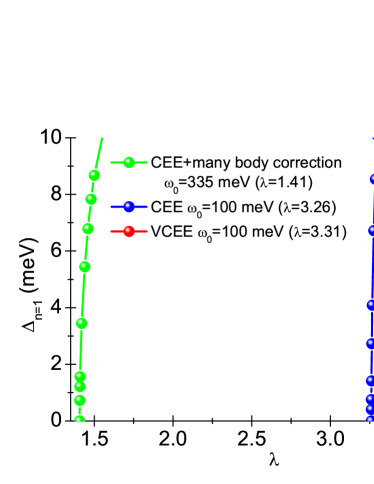
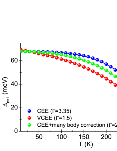
Figure 18: (a) The dependence of maximum value of the order parameter on the electron-phonon coupling constant for C-S-H system ($T_{C}=267$ K and $\mu^{\star}=0.1$). (b) The dependence of order parameter on the temperature. The results has been obtained in the framework of CEE model, VCEE formalism and equations taking into account the additional many-body terms.

References

- Ashcroft (1968) N. W. Ashcroft, Physical Review Letters 21, 1748 (1968).
- McMahon et al. (2012) J. M. McMahon, M. A. Morales, C. Pierleoni, and D. M. Ceperley, Reviews of Modern Physics 84, 1607 (2012).
- Dias and Silvera (2017) R. P. Dias and I. F. Silvera, Science 355, 715 (2017).
- Ashcroft (2004) N. W. Ashcroft, Physical Review Letters 92, 187002 (2004).
- Duan et al. (2014) D. Duan, Y. Liu, F. Tian, X. Huang, Z. Zhao, H. Yu, B. Liu, W. Tian, and T. Cui, Scientific Reports 4, 6968 (2014).
- Drozdov et al. (2015) A. P. Drozdov, M. I. Eremets, I. A. Troyan, V. Ksenofontov, and S. I. Shylin, Nature 525, 73 (2015).
- Drozdov et al. (2014) A. P. Drozdov, M. I. Eremets, and I. A. Troyan, arXiv: 1412.0460 (2014).
- Liu et al. (2017) H. Liu, I. I. Naumov, R. Hoffmann, N. W. Ashcroft, and R. J. Hemley, Proceedings of the National Academy of Sciences 114, 6990 (2017).
- Peng et al. (2017) F. Peng, Y. Sun, C. J. Pickard, R. J. Needs, Q. Wu, and Y. Ma, Physical Review Letters 119, 107001 (2017).
- Kvashnin et al. (2018) A. G. Kvashnin, D. V. Semenok, I. A. Kruglov, I. A. Wrona, and A. R. Oganov, ACS Applied Materials & Interfaces 10, 43809 (2018).
- Ye et al. (2018) X. Ye, N. Zarifi, E. Zurek, R. Hoffmann, and N. W. Ashcroft, The Journal of Physical Chemistry C 122, 6298 (2018).
- Semenok et al. (2020) D. V. Semenok, A. G. Kvashnin, A. G. Ivanova, V. Svitlyk, V. Y. Fominski, A. V. Sadakov, O. A. Sobolevskiy, V. M. Pudalov, I. A. Troyan, and A. R. Oganov, Materials Today 33, 36 (2020).
- Drozdov et al. (2019) A. P. Drozdov, P. P. Kong, V. S. Minkov, S. P. Besedin, M. A. Kuzovnikov, S. Mozaffari, L. Balicas, F. F. Balakirev, D. E. Graf, V. B. Prakapenka, et al., Nature 569, 528 (2019).
- Somayazulu et al. (2019) M. Somayazulu, M. Ahart, A. K. Mishra, Z. M. Geballe, M. Baldini, Y. Meng, V. V. Struzhkin, and R. J. Hemley, Physical Review Letters 122, 027001 (2019).
- Snider et al. (2020) E. Snider, N. Dasenbrock-Gammon, R. McBride, M. Debessai, H. Vindana, K. Vencatasamy, K. V. Lawler, A. Salamat, and R. P. Dias, Nature 586, 373 (2020).
- Durajski et al. (2016) A. P. Durajski, R. Szczȩśniak, and L. Pietronero, Annalen der Physik 528, 358 (2016).
- Kruglov et al. (2020) I. A. Kruglov, D. V. Semenok, H. Song, R. Szczȩśniak, I. A. Wrona, R. Akashi, M. M. D. Esfahani, D. Duan, T. Cui, A. G. Kvashnin, et al., Physical Review B 101, 024508 (2020).
- Hu et al. (2020) S. X. Hu, R. Paul, V. V. Karasiev, and R. P. Dias, arXiv:2012.10259 (2020).
- Hirsch and Marsiglio (2020) J. E. Hirsch and F. Marsiglio, arXiv:2012.12796v1 (2020).
- Dogan and Cohen (2020) M. Dogan and M. L. Cohen, arXiv:2012.10771 (2020).
- Canfield et al. (2003) P. C. Canfield, S. L. Budko, and D. K. Finnemore, Physica C 385, 1 (2003).
- Iye et al. (1988) Y. Iye, T. Tamegai, H. Takeya, and H. Takei, In Superconducting Materials, edited by S. Nakajima and H. Fukuyama (Jpn. J. Appl. Phys. Series I (Publication Office, Japanese Journal of Applied Physics, Tokyo, 1988).
- Hazra et al. (2016) D. Hazra, N. Tsavdaris, S. Jebari, A. Grimm, F. Blanchet, F. Mercier, E. Blanquet, C. Chapelier, and M. Hofheinz, Supercond. Sci. Technol. 29, 10501 (2016).
- Eliashberg (1960) G. M. Eliashberg, Soviet Physics JETP 11, 696 (1960).
- Migdal (1958) A. B. Migdal, Soviet Physics JETP 34, 996 (1958).
- Carbotte (1990) J. P. Carbotte, Reviews of Modern Physics 62, 1027 (1990).
- Freericks et al. (1997) J. K. Freericks, E. J. Nicol, A. Y. Liu, and A. A. Quong, Physical Review B 55, 11651 (1997).
- Mitrovic et al. (1984) B. Mitrovic, H. G. Zarate, and J. P. Carbotte, Physical Review B 29, 184 (1984).
- Kostrzewa et al. (2020) M. Kostrzewa, K. M. Szczȩśniak, A. P. Durajski, and R. Szczȩśniak, Scientific Reports 10, 1592 (2020).
- Troyan et al. (2021) I. A. Troyan, D. V. Semenok, A. G. Kvashnin, A. V. Sadakov, O. A. Sobolevskiy, V. M. Pudalov, A. G. Ivanova, V. B. Prakapenka, E. Greenberg, A. G. Gavriliuk, et al., Advanced Materials 33, 2006832 (2021).
- Errea et al. (2015) I. Errea, M. Calandra, C. J. Pickard, J. Nelson, R. J. Needs, Y. Li, H. Liu, Y. Zhang, Y. Ma, and F. Mauri, Physical Review Letters 114, 157004 (2015).
- Parr and Yang (1989) R. G. Parr and W. Yang, Density-functional theory of atoms and molecules (Oxford University Press, New York, Oxford, 1989).
- Morel and Anderson (1962) P. Morel and P. W. Anderson, Physical Review 125, 1263 (1962).
- Bauer et al. (2012) J. Bauer, J. E. Han, and O. Gunnarsson, Journal of Physics: Condensed Matter 24, 492202 (2012).
- Beach et al. (2000) K. S. D. Beach, R. J. Gooding, and F. Marsiglio, Physical Review B 61, 5147 (2000).
- Pietronero and Strässler (1992) L. Pietronero and S. Strässler, Europhysics Letters 18, 627 (1992).
- Pickett (1993) W. E. Pickett, in Solid State Physics, edited by H. Ehrenreich and F. Spaepan (Academic, New York, 1993).
- Uemura et al. (1991) Y. J. Uemura, L. P. Le, G. M. Luke, B. J. Sternlieb, W. D. Wu, J. H. Brewer, T. M. Riseman, C. L. Seaman, M. B. Maple, M. Ishikawa, et al., Physical Review Letters 66, 2665 (1991).
- Uemura et al. (1992) Y. J. Uemura, L. P. Le, G. M. Luke, B. J. Sternlieb, W. D. Wu, J. H. Brewer, T. M. Riseman, C. L. Seaman, M. B. Maple, M. Ishikawa, et al., Physical Review Letters 68, 2712 (1992).
- D’Ambrumenil (1991) N. D’Ambrumenil, Nature 352, 472 (1991).
- Wojciechowski (1996) R. J. Wojciechowski, paper from: International Centre For Theoretical Physics 28, 1 (1996).
- Goto and Natsume (1996) H. Goto and Y. Natsume, Physica B 216, 281 (1996).
- Metzner and Vollhardt (1989) W. Metzner and D. Vollhardt, Physical Review Letter 62, 324 (1989).
- Freericks and Scalapino (1994) J. K. Freericks and D. J. Scalapino, Physical Review B 49, 6368 (1994).
- Freericks (1994) J. K. Freericks, Physical Review B 50, 403 (1994).
- Freericks and Jarrell (1994) J. K. Freericks and M. Jarrell, Physical Review B 50, 6939 (1994).
- Nicol and Freericks (1994) E. J. Nicol and J. K. Freericks, Physica C 235-240, 2379 (1994).
- Freericks et al. (1996) J. K. Freericks, E. J. Nicol, A. Y. Liu, and A. A. Quong, Czechoslovak Journal of Physics 46, Suppl. S2, 603 (1996).
- Durajski (2016) A. P. Durajski, Scientific Reports 6, 38570 (2016).
- Kostrzewa et al. (2018) M. Kostrzewa, R. Szczȩśniak, J. K. Kalaga, and I. A. Wrona, Scientific Reports 8, 11957 (2018).
- Grimaldi et al. (1995) C. Grimaldi, L. Pietronero, and S. Strässler, Physical Review B 52, 10530 (1995).
- Pietronero et al. (1995) L. Pietronero, S. Strässler, and C. Grimaldi, Physical Review B 52, 10516 (1995).
- Profeta et al. (2012) G. Profeta, M. Calandra, and F. Mauri, Nature Physics 8, 131 (2012).
- Ludbrook et al. (2015) B. M. Ludbrook, G. Levy, P. Nigge, M. Zonno, M. Schneider, D. J. Dvorak, C. N. Veenstra, S. Zhdanovich, D. Wong, P. Dosanjh, et al., PNAS 112, 11795 (2015).
- Zheng and Margine (2016) J. J. Zheng and E. R. Margine, Phys. Rev. B 94, 064509 (2016).
- Szczȩśniak and Szczȩśniak (2019) D. Szczȩśniak and R. Szczȩśniak, Physical Review B 99, 224512 (2019).
- Shimada et al. (2017) N. H. Shimada, E. Minamitani, and S. Watanabe, Applied Physics Express 10, 093101 (2017).
- Szewczyk et al. (2020) K. A. Szewczyk, I. A. Domagalska, A. P. Durajski, and R. Szczȩśniak, Beilstein Journal of Nanotechnology 11, 1178 (2020).
- Perdew et al. (1996) J. P. Perdew, K. Burke, and M. Ernzerhof, Physical Review Letters 77, 3865 (1996).
- Giannozzi et al. (2009) P. Giannozzi, S. Baroni, N. Bonini, M. Calandra, R. Car, C. Cavazzoni, D. Ceresoli, G. L. Chiarotti, M. Cococcioni, I. Dabo, et al., Journal of Physics: Condensed Matter 21, 395502 (2009).
- Giannozzi et al. (2017) P. Giannozzi, O. Andreussi, T. Brumme, O. Bunau, M. B. Nardelli, M. Calandra, R. Car, C. Cavazzoni, D. Ceresoli, M. Cococcioni, et al., Journal of Physics: Condensed Matter 29, 465901 (2017).
- Billeter et al. (2003) S. R. Billeter, A. Curioni, and W. Andreoni, Computational Materials Science 27, 437 (2003).
- Mozaffari et al. (2019) S. Mozaffari, D. Sun, V. S. Minkov, A. P. Drozdov, D. Knyazev, J. B. Betts, M. Einaga, K. Shmizu, M. I. Eremets, L. Balicas, et al., Nature Communications 10, 2522 (2019).
- Togo and Tanaka (2015) A. Togo and I. Tanaka, Scripta Materialia 108, 1 (2015).
- Szczȩśniak (2006) R. Szczȩśniak, Acta Physica Polonica A 109, 179 (2006).
- Bardeen et al. (1957a) J. Bardeen, L. N. Cooper, and J. R. Schrieffer, Physical Review 106, 162 (1957a).
- Bardeen et al. (1957b) J. Bardeen, L. N. Cooper, and J. R. Schrieffer, Physical Review 108, 1175 (1957b).
- Eschrig (2001) H. Eschrig, Theory of Superconductivity: A Primer (Citeseer, 2001).
- Szczȩśniak and Durajski (2013) R. Szczȩśniak and A. P. Durajski, Solid State Sciences 25, 45 (2013).
- Durajski et al. (2020) A. P. Durajski, M. W. Jarosik, K. P. Kosk-Joniec, I. A. Wrona, M. Kostrzewa, K. A. Szewczyk, and R. Szczȩśniak, Acta Physica Polonica A 138, 715 (2020).
- Struzhkin et al. (1997) V. V. Struzhkin, R. J. Hemley, H. Mao, and Y. A. Timofeev, Nature 390, 382 (1997).
- Li et al. (2014) Y. Li, J. Hao, H. Liu, Y. Li, and Y. Ma, The Journal of Chemical Physics 140, 174712 (2014).
- Cui et al. (2020) W. Cui, T. Bi, J. Shi, Y. Li, H. Liu, E. Zurek, and R. J. Hemley, Physical Review B 101, 134504 (2020).
- Li et al. (2015) Y. Li, J. Hao, H. Liu, J. S. Tse, Y. Wang, and Y. Ma, Scientific Reports 5, 9948 (2015).
- Durajski et al. (2015) A. P. Durajski, R. Szczȩśniak, and Y. Li, Physica C 515, 1 (2015).
- Errea et al. (2016) I. Errea, M. Calandra, C. J. Pickard, J. R. Nelson, R. J. Needs, Y. Li, H. Liu, Y. Zhang, Y. Ma, and F. Mauri, Nature 532, 81 (2016).
- Durajski and Szczȩśniak (2017) A. P. Durajski and R. Szczȩśniak, Scientific Reports 7, 4473 (2017).
- Tanaka et al. (2017) K. Tanaka, J. S. Tse, and H. Liu, Physical Review B 96, 100502 (2017).
- Heil et al. (2019) C. Heil, S. di Cataldo, G. B. Bachelet, and L. Boeri, Physical Review B 99, 220502(R) (2019).
- Durajski et al. (2012) A. P. Durajski, R. Szczȩśniak, and M. W. Jarosik, Phase Transitions 85, 727 (2012).
- Yan et al. (2011) Y. Yan, J. Gong, and Y. Liu, Physics Letters A 375, 1264 (2011).
- Durajski et al. (2014) A. Durajski, R. Szczȩśniak, and A. Duda, Solid State Communications 195, 55 (2014).
- Szczȩśniak and Jarosik (2009) R. Szczȩśniak and M. Jarosik, Solid State Communications 149, 2053 (2009).
- Kostrzewa et al. (2021) M. Kostrzewa, A. P. Durajski, J. K. Kalaga, and R. Szczȩśniak, Journal of Superconductivity and Novel Magnetism xxx, xxx (2021).
- Fetter and Walecka (1971) A. L. Fetter and J. D. Walecka, Quantum Theory of Many-Particle Systems (McGraw-Hill Book Company, 1971).
- Elk and Gasser (1979) K. Elk and W. Gasser, Die Methode der Greenschen Funktionen in der Festkörperphysik (Akademie - Verlag, 1979).