Robust Inference on Income Inequality:
t-Statistic Based Approaches

Abstract

Empirical analyses on income and wealth inequality and those in other fields in economics and finance often face the difficulty that the data is heterogeneous, heavy-tailed or correlated in some unknown fashion. The paper focuses on applications of the recently developed t-statistic based robust inference approaches in the analysis of inequality measures and their comparisons under the above problems. Following the approaches, in particular, a robust large sample test on equality of two parameters of interest (e.g., a test of equality of inequality measures in two regions or countries considered) is conducted as follows: The data in the two samples dealt with is partitioned into fixed numbers $q_{1},q_{2}\geq 2$ (e.g., $q_{1}=q_{2}=2,4,8$) of groups, the parameters (inequality measures dealt with) are estimated for each group, and inference is based on a standard two-sample $t-$test with the resulting $q_{1},q_{2}$ group estimators. Robust $t-$statistic approaches result in valid inference under general conditions that group estimators of parameters (e.g., inequality measures) considered are asymptotically independent, unbiased and Gaussian of possibly different variances, or weakly converge, at an arbitrary rate, to independent scale mixtures of normal random variables. These conditions are typically satisfied in empirical applications even under pronounced heavy-tailedness and heterogeneity and possible dependence in observations. The methods dealt with in the paper complement and compare favorably with other inference approaches available in the literature. The use of robust inference approaches is illustrated by an empirical analysis of income inequality measures and their comparisons across different regions in Russia.

Keywords: Income inequality, inequality measures, robust inference, heavy-tailedness, Russian economy.

JEL Codes: C14, D31, D63

1 Introduction

Empirical analyses on income and wealth inequality and those in other fields in economics and finance often face the difficulty that the data is heterogeneous, heavy-tailed or correlated in some unknown fashion (see, among others, the discussion and reviews in

Importantly, many studies going back to V. Pareto indicate that income and wealth distributions are heavy-tailed and follow power laws

$$P(X>x)\sim Cx^{-\zeta},\;\;C>0,$$ (1)

with the tail index $\zeta>0$ (see, among others, the discussion and reviews in Piketty and Saez, 2003, Atkinson, 2008, Gabaix, 2009, Milanovic, 2005, 2011, Atkinson and Piketty, 2010, Atkinson et al., 2011, Toda, 2012, Ibragimov et al., 2015, Gabaix et al., 2016, Ibragimov and Ibragimov, 2018, Toda and Wang, 2020, and references therein).

Typical empirical results are $\zeta\in(1.5,3)$ for income, and $\zeta\approx 1.5$ for wealth. Thus, the variance is infinite for wealth and may be infinite for income.

More generally, the tail index parameter $\zeta$ of power law distributions (1) characterize the heaviness (the rate of decay) of its tails, with smaller values of $\zeta$ corresponding to more pronounced heavy-tailedness in the distributions, and vice versa. The tail index $\zeta$ governs the likelihood of observing outliers and extreme values of $X,$ e.g., very high income/wealth levels in the case of income and wealth distributions. It is further important as it governs existence of moments of the r.v. $X>0,$ with the moment $EX^{p}$ of order $p>0$ of $X$ being finite if and only if $\zeta>p.$ In particular, the second moment $EX^{2}$ of the r.v. $X$ is finite and its variance $Var(X)$ is defined if and only if $\zeta>2,$ and the first moment - the mean $EX$- of $X$ is finite if and only if $\zeta>1.$

Applicability of commonly used approaches to inference on inequality measures based on asymptotic normality becomes problematic under heavy-tailedness, heterogeneity and correlation in the data. For instance, sample inequality measures - estimators of measures of inequality like sample Gini coefficient - converge to non-Gaussian limits given by stable random variables (r.v.’s) under sufficiently pronounced heavy-tailedness with infinite second moments and variances (see Fontanari et al. (2018) and the discussion in Appendix B).

Provided normal convergence for sample inequality measures holds, asymptotic methods based on it often have poor finite sample properties under the problems of extreme values, outliers and heavy-tailedness in data. Similar problems are also observed for bootstrap methods (see Cowell and Flachaire, 2007, Davidson and Flachaire, 2007). Bootstrap methods are also known to fail in heavy-tailed infinite variance settings (see the discussion in Section 5 in Davidson and Flachaire, 2007, and references therein).

The problems with inference on inequality measures are discussed in detail in Dufour et al. (2019, 2020). These works also emphasize that reliable methods remain scarce for both the one-sample problem of inference on a single inequality index and the two-sample problem of testing for equality of and inference on the difference between two inequality indices. As discussed in Dufour et al. (2019, 2020), the latter problem is much more challenging than the former (see also Ibragimov and Müller, 2016, for the discussion and the results on robust inference on equality of and the difference between two general parameters of interest under heterogeneity and dependence). Dufour et al. (2019) propose permutation tests for the hypothesis of equality of two inequality measures from independent samples which outperforms other asymptotic and bootstrap methods available in the literature (see also Canay et al., 2017, for permutation tests of equality of two general parameters of interest under heterogeneity and clustered dependence). As discussed in Dufour et al. (2020), the latter tests for the two-sample problem for inequality indices are limited to testing the equality of two inequality measures. In particular, they do not provide a way of making inference on a possibly non-zero difference between the two measures considered nor building a confidence interval for the difference.

Dufour et al. (2020) propose Fieller-type methods for inference on the generalized entropy (GE) class of inequality measures. Among other results, the authors develop approaches to testing and construction of confidence intervals for any possibly non-zero difference between the inequality measures that can be used under independent samples of i.i.d. observations with possibly unequal sizes and equal-sized samples of i.i.d. observation with arbitrary dependence between the samples.

This paper focuses on applications of recently developed $t-$statistic approaches (see Ibragimov and Müller, 2010, 2016, and also Ch. 3 in Ibragimov et al., 2015) in robust inference on income and wealth inequality measures under the problems of heterogeneity, heavy-tailedness and possible dependence in observations. Following the approaches, in particular, a robust large sample test on equality or a non-zero difference of two parameters of interest (e.g., a test of equality of inequality measures in two regions or countries considered) is conducted as follows: The data in the two samples dealt with is partitioned into fixed numbers $q_{1},q_{2}\geq 2$ (e.g., $q_{1}=q_{2}=2,4,8$) of groups, the parameters (inequality measures dealt with) are estimated for each group, and inference is based on a standard two-sample $t-$test with the resulting $q_{1},q_{2}$ group estimators (see the next section). As follows from the results in Ibragimov and Müller (2010, 2016), robust $t-$statistic approaches result in valid inference under general conditions that group estimators of parameters of interest (e.g., inequality measures) considered weakly converge, at an arbitrary rate, to independent normal or scale mixtures of normal r.v.’s. These conditions are typically satisfied in empirical applications even under pronounced heavy-tailedness, heterogeneity and possible dependence in observations. The approaches proposed in the paper complement and compare favorably with other inference methods available in the literature, including computationally expensive bootstrap procedures and permutation-based inference methods. Importantly, the approaches proposed in the paper can be used in testing and construction of confidence intervals for any possibly non-zero difference between inequality measures under the problems of heterogeneity, heavy-tailedness and possible dependence in the data.

One should also emphasize wider range of applicability of $t-$statistic approaches to inference on inequality measures proposed in the paper as compared to other inference methods available in the literature, including those considered in Dufour et al. (2019, 2020). The inference approaches can be used in the case where observations (e.g., on income or wealth levels) in each of the samples considered are dependent among themselves - for instance, due to spatial or clustered dependence (see Conley (1999) and Bhattacharya (2007) for a review of settings and methods of inference under spatial and clustered dependence, including complex stratified and clustered household surveys), common shocks affecting them (see Andrews (2005) and Hwang (2021) for a review of and inference using data with common shock dependence), or, in the case of time series or panel data on income or wealth levels, due to autocorrelation and dependence in observations over time. Further, in the case of testing for equality of inequality measures or inference on their difference in two populations using two samples of possibly dependent observations, as above, the $t-$statistic inference approaches may be used under an arbitrary dependence between the samples as well as under possibly unequal sample sizes.

Application of the robust inference approaches is illustrated by an empirical analysis of income inequality measures and their comparisons across different regions in Russia.

The paper is organized as follows. Section 2 describes the robust $t-$statistic approaches to inference on inequality measures analyzed in the paper and discusses the conditions for their validity. Section 3 provides numerical results on finite sample performance of the robust inference approaches dealt with and their comparisons with other inference methods in the literature, with a particular focus on testing equality of two inequality measures and inference on the difference between two inequality indices in Section 3.2. Section 4 presents empirical applications of the robust $t-$statistic approaches in the analysis of income inequality in Russia and comparisons of inequality measures across Russian regions. Section 5 makes some concluding remarks and discusses some suggestions for future research. Appendix A provides tables on the numerical and empirical results in the paper. Appendix B provides a review of the definitions and asymptotic properties of the Gini, Theil and Generalized Entropy measures referred to in the paper and a discussion of applicability of the robust approaches dealt with in inference on the measures.

2 Methodology: Robust t-statistic approaches to inference on inequality measures

We focus on inference on inequality measures using the t-statistic approaches to robust inference under heterogeneity, heavy-tailedness and dependence of largely unknown form recently developed in Ibragimov and Müller (2010, 2016). Ibragimov and Müller (2010) provide an approach to robust inference on an arbitrary single parameter of interest. Ibragimov and Müller (2016) provide approaches to robust testing of equality of two arbitrary parameters of interest and to robust inference on the difference of the parameters.

We refer to, among others, Section 13.F in Cowell and Flachaire (2007), Davidson and Flachaire (2007), Marshall et al. (2011), Ibragimov and Ibragimov (2018), Dufour et al. (2019) and Dufour et al. (2020) for definitions of the most widely inequality measures, including Gini, Generalized Entropy and Theil indices, and their values for different income distributions, including empirically relevant heavy-tailed Pareto, double Pareto and Singh-Maddala distributions (see the next section).

In the context of a one-sample inference on a single (income or wealth) inequality (e.g., a Theil, Generalized entropy - GE - or Gini index) the robust $t-$statistic approaches are implemented as follows.

Throughout the paper, we denote by $T_{k}$ a r.v. that has a Student-$t$ distribution with $k\geq 1$ degrees of freedom. Further, for $q\geq 2$ and $0<\alpha<1,$ by $cv_{q,\alpha}$ we denote the $(1-\alpha/2)-$quantile of the Student-$t$ distribution with $q-1$ degrees of freedom: $P(\left|T_{q-1}\right|>t_{\alpha}$)= $\alpha$.

Consider the one-sample problem of testing a hypothesis on or constructing a confidence interval for an inequality measure $\mathcal{L}.$ Following the $t-$statistic robust inference approaches in Ibragimov and Müller (2010), a (large) sample I₁, I₂,…, I_N of observations on income or wealth levels $I,$ is partitioned into a fixed number $q\geq 2$ (e.g., $q=2,4$ or 8) of groups, and the income inequality measure $\mathcal{L}$ is estimated using the data for each group thus resulting in $q$ group empirical income inequality measures ${\widehat{\mathcal{L}}}_{j}$, $j=1,...,q.$ The robust test of the null hypothesis $H_{0}:\mathcal{L}={\mathcal{L}}_{0}$ against the two-sided alternative $H_{a}:\mathcal{L}\neq{\mathcal{L}}_{0}$ is based on the usual $t-$statistic $t^{I}_{\mathcal{L}}$ in the $q$ group empirical inequality measures ${\widehat{\mathcal{L}}}_{j}$, $j=1,...,q:$

$$t_{\mathcal{L}}=\sqrt{q}\frac{\overline{\widehat{\mathcal{L}}}-{\mathcal{L}}_{0}}{s_{\widehat{\mathcal{L}}}}$$ (2)

with $\overline{\widehat{\mathcal{L}}}=\frac{\sum^{q}_{j=1}{{\widehat{\mathcal{L}}}_{j}}}{q}$ and $s^{2}_{\widehat{\mathcal{L}}}=\frac{\sum^{q}_{j=1}{{\left({\widehat{\mathcal{L}}}_{j}-\overline{\widehat{\mathcal{L}}}\right)}^{2}}}{q-1}$ ${\widehat{\mathcal{L}}}_{j}.$ The above null hypothesis $H_{0}$ is rejected in favor of the alternative $H_{a}$ at level $\alpha\leq 0.83$ (e.g., at the usual significance level $\alpha=0.05$) if the absolute value $|t_{\mathcal{L}}|$ of the $t-$statistic in group estimates ${\widehat{\mathcal{L}}}_{j}$ exceeds the $(1-\alpha/2)-$quantile of the standard Student-$t$ distribution with $q-1$ degrees of freedom: $|t_{\mathcal{L}}|>cv_{q,\alpha}.$ The test of $H_{0}$ against $H_{a}$ of level $\alpha\leq 0.1$ is conducted in the same way if $2\leq q\leq 14.$ Using the results in Bakirov and Székely (2006) and Ibragimov and Müller (2010), one can further calculate the $p-$values of the above $t-$statistic robust tests in the case of an arbitrary number $q$ of groups thus enabling conducting robust tests on the inequality measure $\mathcal{L}$ of an arbitrary level.

By implication, for all $\alpha\leq 0.83$ (and all $\alpha\leq 0.1$ for $2\leq q\leq 14$) a confidence interval for the inequality measure $\mathcal{L}$ with asymptotic coverage of at least $1-\alpha$ may be constructed as ${\widehat{\mathcal{L}}}_{j}\pm cv_{q,\alpha}s_{\widehat{\mathcal{L}}}.$ For instance, the 95% confidence interval for $\mathcal{L}$ is given by $(\overline{\widehat{\mathcal{L}}}-cv_{q,0.05}s_{\widehat{\mathcal{L}}}\mathrm{,\ \ }\overline{\widehat{\mathcal{L}}}+cv_{q,0.05}s_{\widehat{\mathcal{L}}}$), where cv_q,0.05 is the 0.975-quantile of the Student-t distribution with q$-$1 degrees of freedom: $P(\left|T_{q-1}\right|>cv_{q,0.05}$)=0.05.

As follows from Ibragimov and Müller (2010), the above approach results in asymptotically valid inference under the assumption that the group empirical income inequality measures ${\widehat{\mathcal{L}}}_{j}$, $j=1,...,q,$ are asymptotically independent, unbiased and Gaussian of possibly different variances.

The asymptotic validity of the t-statistic based inference approach continues to hold even when the group estimators ${\widehat{\mathcal{L}}}_{j}$ of $\mathcal{L}$ converge (at an arbitrary rate) to independent but potentially heterogeneous scale mixtures of normal r.v.’s, such as heavy-tailed stable symmetric r.v.’s. It also holds under convergence of the group estimators to conditionally normal r.v.’s which are unconditionally dependent through their second moments or have a common shock-type dependence (see Andrews, 2005, for inference methods under common shock dependence structures, and Hwang, 2021, for applications of $t-$statistic robust inference approaches in such settings). This implies that the t-statistic based robust inference on $\mathcal{L}$ can thus be applied under extremes and outliers in observations generated by heavy-tailedness with infinite variances and, among others, dependence structures that include models with multiplicative common shocks (see Ibragimov, 2007, 2009). The $t-$statistic based approaches do not require at all estimation of limiting variances of estimators of interest, in contrast to inference methods based on consistent, e.g., HAC or clustered, standard errors (see Section 1). The numerical analysis in Ibragimov and Müller (2007, 2016) and Section 3 in Ibragimov et al. (2015) indicates favorable finite sample performance of the $t-$statistic based robust inference approaches in inference on models with time series, panel, clustered and spatially correlated data. See also Esarey and Menger (2019) for a detailed numerical analysis of finite sample performance of different inference procedures, including $t-$statistic and related approaches, under small number of clusters of dependent data and their software (STATA and R) implementation.

The above conditions for asymptotic validity of $t-$statistic approaches to robust inference are typically satisfied in applications, under the appropriate choice of the groups implying asymptotic unbiasedness and independence of group estimators of parameters of interest - inequality measures considered (see below). Namely, the asymptotic Gaussianity (or other weak convergence results, e.g., convergence to heavy-tailed scale mixtures of Gaussian distributions) of group estimators - group empirical inequality measures - ${\widehat{\mathcal{L}}}_{j}$ typically follows from the same reasoning and holds under the same conditions as the asymptotic Gaussianity (or other relevant asymptotics) of the full-sample estimator - full-sample empirical inequality measure - ${\widehat{\mathcal{L}}}.$

Concerning the choice of the groups, the condition that group estimators of parameters of interest - inequality measures dealt with - should be asymptotically unbiased (and independent) places natural - again typically satisfied in applications - restrictions on formation of groups in applications of $t-$statistic approaches in the context of inference on inequality indices and their comparisons (see also discussion of general $t-$statistic inference approaches in Ibragimov and Müller, 2010). For instance, in the problem of inference on a single inequality measure in the whole country, e.g., Russia, using household income surveys with random samples of households in the country and its regions and thus i.i.d data on income levels, groups cannot be chose to be the country regions. This is because each of the group estimators - group inequality measures - will estimate the inequality index considered in the corresponding region but not in the whole country and unbiasedness of the group estimators with the mean asymptotically equal to the country’s inequality index of interest will not hold. The ‘‘between-region’’ component of inequality in the whole country would be missed out by the group estimators.

On the other hand, in the problem of testing equality of or inference on the difference between inequality indices in two regions of a country, e.g., Russia as in the empirical application in Section 4 in this paper, using household income surveys with i.i.d. data on household income levels in the regions considered, the groups in applications of two-sample $t-$statistic approaches can be formed just by taking subsequent observations on incomes in the two samples of i.i.d. income data in the regions (similar to applications of the approaches with time series data, see Ibragimov and Müller, 2010). Namely, in the case of inference on equality of inequality indices of interest in two regions using the random samples $I_{1},I_{2},...,I_{N_{1}},$ $Y_{1},Y_{2},...,Y_{N_{2}}$ of (i.i.d.) income levels in them, the $q_{1},q_{2}$ groups in applications of two-sample $t-$statistic approaches based on $\tilde{t}_{\mathcal{L}}$ in (3) can be taken to be the groups $\{I_{k},(i-1)N_{1}/q_{1}<k\leq iN_{1}/q_{1}\},$ $\{Y_{l},(j-1)N_{2}/q_{2}<l\leq jN_{2}/q_{2}\},$ $i=1,...,q_{1},$ $j=1,...,q_{2},$ of subsequent observations on household incomes in the samples considered. The groups of subsequent observations in the two samples in applications of $t-$statistic approaches based on $\tilde{\tilde{t}}_{\mathcal{L}}$ in (4) with $q_{1}=q_{2}=q$ are formed in a similar way. With the above simple choice of groups, asymptotic unbiasedness and independence of group estimators - group inequality measures - holds due to i.i.d.ness of data in the random samples considered.

Let us now turn to testing that the values $L_{1}$ and $L_{2}$ of an inequality measure $\mathcal{L}$ are equal in two populations (e.g., for income distributions in two regions of a country) and to inference on the difference $d=L_{1}-L_{2}$ between the two inequality indices using the (large) samples $I_{1},I_{2},...,I_{N_{1}}$ and $Y_{1},Y_{2},...,Y_{N_{2}}$ on income or wealth levels in the populations. We first assume that the two samples are independent. Following the $t-$statistic approaches to robust inference on two parameters of interest in Ibragimov and Müller (2016), each of the two samples $I_{1},I_{2},...,I_{N_{1}}$ and $Y_{1},Y_{2},...,Y_{N_{2}}$ is partitioned into fixed numbers $q_{1},q_{2}\geq 2$ (e.g., $q_{1},q_{2}=2,4$ or 8) groups, respectively, and the income inequality measure $\mathcal{L}$ is estimated using the data for each of the groups in the two samples. This thus results in $q_{1}+q_{2}$ group empirical income inequality measures ${\widehat{\mathcal{L}}}^{I}_{1},$ …, ${\widehat{\mathcal{L}}}^{I}_{q_{1}},$ and ${\widehat{\mathcal{L}}}^{Y}_{1}$, …, ${\widehat{\mathcal{L}}}^{Y}_{q_{2}}.$ The robust test of the null hypothesis $H_{0}:L_{1}-L_{2}=d_{0}$ (e.g., with $d_{0}=0,$ the test of the hypothesis $H_{0}:L_{1}=L_{2}$ of equality of the values $L_{1},L_{2}$ of the inequality index $\mathcal{L}$ in the two populations considered) against the two-sided alternative $H_{a}:L_{1}-L_{2}\neq d_{0}$ (resp., with $d_{0}=0,$ against the two-sample alternative $H_{a}:L_{1}\neq L_{2}$) is based on the usual two-sample $t-$statistic $\tilde{t}_{\mathcal{L}}$ in the $q_{1}+q_{2}$ group empirical inequality measures ${\widehat{\mathcal{L}}}^{I}_{j}$, ${\widehat{\mathcal{L}}}^{Y}_{k}$, $j=1,...,q_{1},$ $k=1,...,q_{2}:$

$$\tilde{t}_{\mathcal{L}}=\frac{\overline{\widehat{\mathcal{L}}^{I}}-\overline{\widehat{\mathcal{L}}^{Y}}-d_{0}}{\sqrt{s^{2}_{\widehat{\mathcal{L}}^{I}}/q_{1}+s^{2}_{\widehat{\mathcal{L}}^{Y}}/q_{2}}}$$ (3)

with

$$\overline{\widehat{\mathcal{L}}^{I}}=\frac{1}{q_{1}}\sum^{q_{1}}_{j=1}{{\widehat{\mathcal{L}}}^{I}_{j}},\overline{\widehat{\mathcal{L}}^{Y}}=\frac{1}{q_{2}}\sum^{q_{2}}_{k=1}{{\widehat{\mathcal{L}}}^{Y}_{k}},$$

$$s^{2}_{\widehat{\mathcal{L}}^{I}}=\frac{1}{q_{1}-1}\sum^{q_{1}}_{j=1}{\left({\widehat{\mathcal{L}}}^{I}_{j}-\overline{\widehat{\mathcal{L}}^{I}}\right)^{2}},s^{2}_{\widehat{\mathcal{L}}^{Y}}=\frac{1}{q_{2}-1}\sum^{q_{2}}_{k=1}{{\left({\widehat{\mathcal{L}}}^{Y}_{k}-\overline{\widehat{\mathcal{L}}^{Y}}\right)}^{2}}.$$

For the number of groups $q_{1},q_{2}\leq 14$ the above null hypothesis $H_{0}:L_{1}-L_{2}=d_{0}$ is rejected in favor of the alternative $H_{a}:L_{1}-L_{2}\neq d_{0}$ (resp., with $d_{0}=0,$ the null hypothesis $H_{0}:L_{1}=L_{2}$ of equality of the inequality measures values in the populations is rejected in favor of the alternative $H_{a}:L_{1}\neq L_{2}$) at level $\alpha\in\{0.001,0.002,...,0.099,0.10\}$ (e.g., at the usual significance levels $\alpha=0.01,0.05$ and 0.1) if the absolute value $|\tilde{t}_{\mathcal{L}}|$ of the two-sample $t-$statistic in group empirical inequality measures ${\widehat{\mathcal{L}}}^{I}_{j}$, ${\widehat{\mathcal{L}}}^{Y}_{k}$, $j=1,...,q_{1},$ $k=1,...,q_{2},$ exceeds the $(1-\alpha/2)-$quantile of the standard Student-$t$ distribution with $q-1$ degrees of freedom, where $q=\min(q_{1},q_{2}):$ $|\tilde{t}_{\mathcal{L}}|>cv_{q,\alpha}=cv_{\min(q_{1},q_{2}),\alpha}.$

One further obtains that, for $\alpha=0.01,0.05,0.1$ and the number of groups $q_{1},q_{2}\leq 14,$ $\min(q_{1},q_{2})=q,$ a confidence interval for the difference $d_{0}=L_{1}-L_{2}$ between the values of the inequality measure $\mathcal{L}$ in two populations with asymptotic coverage of at least $1-\alpha$ may be constructed as
${\widehat{\mathcal{L}}}^{I}-{\widehat{\mathcal{L}}}^{Y}\pm cv_{q,\alpha}\sqrt{s^{2}_{\widehat{\mathcal{L}}^{I}}/q_{1}+s^{2}_{\widehat{\mathcal{L}}^{Y}}/q_{2}}.$ For instance, the 95% confidence interval for $\mathcal{L}$ is given by ${\widehat{\mathcal{L}}}^{I}-{\widehat{\mathcal{L}}}^{Y}\pm cv_{q,0.05}\sqrt{s^{2}_{\widehat{\mathcal{L}}^{I}}/q_{1}+s^{2}_{\widehat{\mathcal{L}}^{Y}}/q_{2}},$ where $cv_{q,0.05}$ is the 0.975-quantile of the Student-t distribution with $\min(q_{1},q_{2})-1$ degrees of freedom: $P(\left|T_{\min(q_{1},q_{2})-1}\right|>cv_{q,0.05}$)=0.05.

As follows from Ibragimov and Müller (2016), the two-sample $t-$statistic approach is asymptotically valid under the assumption - as above, typically satisfied in applications - that the group empirical income inequality measures ${\widehat{\mathcal{L}}}^{I}_{j}$, $j=1,...,q_{1},$ ${\widehat{\mathcal{L}}}^{Y}_{k}$, $k=1,...,q_{2},$ are asymptotically independent, unbiased and Gaussian of possibly different variances (or converge at an arbitrary rate to independent but potentially heterogeneous scale mixtures of normal r.v.’s, such as heavy-tailed stable symmetric r.v.’s).

Let us now consider the problem of testing for equality of the values $L_{1}$ and $L_{2}$ of an inequality measure $\mathcal{L}$ and to inference on the difference $d=L_{1}-L_{2}$ between the inequality indices in two populations using income or wealth level samples $I_{1},I_{2},...,I_{N_{1}}$ and $Y_{1},Y_{2},...,Y_{N_{2}}$ of possibly unequal sizes $N_{1},N_{2}$ that may exhibit an arbitrary dependence between them. Suppose that the samples are divided into an equal number $q_{1}=q_{2}=q\geq 2$ (e.g., $q_{1},q_{2}=2,4$ or 8) of groups, and the sample inequality measures - estimates of the inequality index $\mathcal{L}$ of interest - are calculated using the data for each of the $2q$ groups in the two samples. One thus has the group empirical income inequality measures ${\widehat{\mathcal{L}}}^{I}_{1},$ …, ${\widehat{\mathcal{L}}}^{I}_{q},$ and ${\widehat{\mathcal{L}}}^{Y}_{1}$, …, ${\widehat{\mathcal{L}}}^{Y}_{q}.$ The robust test of the null hypothesis $H_{0}:L_{1}-L_{2}=d_{0}$ (e.g., with $d_{0}=0,$ the test of the hypothesis $H_{0}:L_{1}=L_{2}$ of equality of the values $L_{1},L_{2}$ of the inequality index $\mathcal{L}$ in the two populations) against the two-sided alternative $H_{a}:L_{1}-L_{2}\neq d_{0}$ (resp., with $d_{0}=0,$ against the two-sample alternative $H_{a}:L_{1}\neq L_{2}$) may be based on the one-sample $t-$statistic $\tilde{\tilde{t}}_{\mathcal{L}}$ in the $q$ differences ${\widehat{\mathcal{L}}}^{I}_{j}-{\widehat{\mathcal{L}}}^{Y}_{j},$ $j=1,...,q,$ of the calculated group empirical inequality measures:

$$\tilde{\tilde{t}}_{\mathcal{L}}=\sqrt{q}\frac{\overline{\widehat{\mathcal{L}}^{I}}-\overline{\widehat{\mathcal{L}}^{Y}}-d_{0}}{s_{\widehat{\mathcal{L}}^{I-Y}}}$$ (4)

with

$$\overline{\widehat{\mathcal{L}}^{I}}=\frac{1}{q}\sum^{q}_{j=1}{{\widehat{\mathcal{L}}}^{I}_{j}},\overline{\widehat{\mathcal{L}}^{Y}}=\frac{1}{q}\sum^{q}_{j=1}{{\widehat{\mathcal{L}}}^{Y}_{j}},$$

$$s^{2}_{\widehat{\mathcal{L}}^{I-Y}}=\frac{1}{q-1}\sum^{q}_{j=1}{\left(({\widehat{\mathcal{L}}}^{I}_{j}-{\widehat{\mathcal{L}}}^{Y}_{j})-(\overline{\widehat{\mathcal{L}}^{I}}-\overline{\widehat{\mathcal{L}}^{Y}})\right)^{2}}.$$

As in the case of $t-$statistic inference on one parameter, for any $\alpha\leq 0.83$ (any $\alpha\leq 0.1$ for $2\leq q\leq 14$), the null hypothesis $H_{0}:L_{1}-L_{2}=d_{0}$ (for $d_{0}=0,$ the null hypothesis $H_{0}:L_{1}=L_{2}$ of equality of the values $L_{1},L_{2}$ of the inequality index $\mathcal{L}$ in two populations) is rejected in favor of the two-sided alternative $H_{a}:L_{1}-L_{2}\neq d_{0}$ (resp., for $d_{0}=0,$ in favor of the alternative $H_{a}:L_{1}\neq L_{2}$) at level $\alpha$ if the absolute value $|\tilde{\tilde{t}}_{\mathcal{L}}|$ of the $t-$statistic in the differences ${\widehat{\mathcal{L}}}^{I}_{j}-{\widehat{\mathcal{L}}}^{Y}_{j},$ $j=1,...,q$ of group sample inequality measures exceeds the $(1-\alpha/2)-$quantile of the standard Student-$t$ distribution with $q-1$ degrees of freedom: $|\tilde{\tilde{t}}_{\mathcal{L}}|>cv_{q,\alpha}.$ Further, as in the case of $t-$statistic inference on a single inequality measure, the $p-$values of the above tests can be calculated in the case of an arbitrary number $q=q_{1}=q_{2}$ of groups thus enabling conducting robust tests of an arbitrary level.

For all $\alpha\leq 0.83$ (and all $\alpha\leq 0.1$ for $2\leq q\leq 14$) a confidence interval for the difference $d_{0}=L_{1}-L_{2}$ between the values of the inequality measure $\mathcal{L}$ in two populations with asymptotic coverage of at least $1-\alpha$ may be constructed as ${\widehat{\mathcal{L}}}^{I}_{j}-{\widehat{\mathcal{L}}}^{Y}_{j}\pm cv_{q,\alpha}s_{\widehat{\mathcal{L}}^{I-Y}}.$ For instance, the 95% confidence interval for $\mathcal{L}$ is given by $({\widehat{\mathcal{L}}}^{I}_{j}-{\widehat{\mathcal{L}}}^{Y}_{j}-cv_{q,0.05}s_{\widehat{\mathcal{L}}^{I-Y}},{\widehat{\mathcal{L}}}^{I}_{j}+{\widehat{\mathcal{L}}}^{Y}_{j}-cv_{q,0.05}s_{\widehat{\mathcal{L}}^{I-Y}}),$ where cv_q,0.05 is the 0.975-quantile of the Student-t distribution with q$-$1 degrees of freedom: $P(\left|T_{q-1}\right|>cv_{q,0.05}$)=0.05.

As above, the $t-$statistic approaches to robust inference based on (4) are asymptotically valid under the assumption that the group empirical income inequality measures ${\widehat{\mathcal{L}}}^{I}_{j}$, ${\widehat{\mathcal{L}}}^{Y}_{j}$, $j=1,...,q,$ are asymptotically independent across $j$, unbiased and Gaussian of possibly different variances (or have limiting scale mixtures of Gaussian distributions).

3 Finite sample performance

In this section, we provide numerical results on finite sample properties of the asymptotic, robust $t-$statistic, bootstrap and permutation approaches to inference and tests on inequality measures. The results are provided for inference on Theil and Gini inequality, similar to the numerical analysis in Cowell and Flachaire (2007) and Dufour et al. (2019).

We first present the results for the one-sample problem of inference on a single inequality measure in Section 3.1.

Then, in Section 3.2, the numerical results are provided for the two-sample problem of tests on equality of two inequality measures and inference on the difference between two inequality indices.

As in Dufour et al. (2019), the numerical analysis of finite-sample performance of different approaches to inference on inequality measure(s) is based on simulations from Singh-Maddala distributions that were reported to provide a good fit to real-world income distributions in various countries (see the discussion in Cowell and Flachaire, 2007, Davidson and Flachaire, 2007, Dufour et al., 2019, and references therein). The cdf of the Singh-Maddala distribution with the scale parameter $b>0$ and the shape parameters $a,c>0$ is given by

$$F(x)=1-\left[1+\left(\frac{x}{b}\right)^{a}\right]^{-c},x>0,$$ (5)

(see the above references). Similar to Dufour et al. (2019), the Singh-Madalla distribution with parameters $a,b,c>0$ is denoted by $SM(a,b,c)$ in what follows. It is easy to see that the cdf $F(x)$ of the Singkh-Maddala distribution $SM(a,b,c)$ satisfies $F(x)\sim c\left(\frac{x}{b}\right)^{a}$ as $x\rightarrow 0,$ and $1-F(x)\sim\left(\frac{x}{b}\right)^{-ac}$ as $x\rightarrow\infty.$ Therefore, the Singh-Maddala distribution has the (double) power law or (double) Pareto behavior in the lower tails - for small income levels - and the upper tails - for high incomes (see Toda, 2012, for the analysis of double Pareto and related distributions for income).

In particular, the Singh-Maddala distributions belong to the class of distributions with heavy power law tails, so that for for large $x>0$ and r.v.’s (income or wealth levels) $X>0$ with the Singh-Maddala distribution $SM(a,b,c)$ follows power law (1) with the tail index $\zeta=ac.$

Following Dufour et al. (2019), in the numerical experiments, we use the parameter values $a_{0}=2.8,$ $b_{0}=100^{-1/2.8},$ $c_{0}=1.7$ for the Singh-Maddala distribution, with the corresponding tail index $\zeta=a_{0}c_{0}=4.76,$ as a benchmark. The Theil index for this distribition equals to 0.1401151, and the Gini index equals to 0.2887138 (see Dufour et al., 2019). The Singh-Maddala distribution with the above values for the parameters was also used in Cowell and Flachaire (2007) and Davidson and Flachaire (2007) to demonstrate poor finite-sample performance of asymptotic and bootstrap inference approaches.

Further, as in Dufour et al. (2019), in the numerical experiments, we consider several other Singh-Maddala distributions $SM(a,b_{0},c)$ with the above scale parameter $b_{0}=100^{-1/2.8}$ for which the Theil inequality index and the Gini index are the same as in the case of the distribution $SM(a_{0},b_{0},c_{0}),$ and equal to 0.1401151 (the Theil index) and 0.2887138 (the Gini index).

Following Dufour et al. (2019), in simulations involving the Theil index, we take the parameters $(a,c)$ of the Singh-Maddala distributions $SM(a,b_{0},c)$ equal to $(2.5,2.502199),$ $(2.6,2.149747),$ $(2.7,1.894309),$ $(2.8,1.7),$ $(3.0,1.4223847),$ $(3.2,1.2320215),$ $(3.4,1.0922125),$ $(3.8,0.8984488),$
$(4.8,0.6366578)$ and $(5.8,0.4996163).$ The corresponding tail indices $\zeta$ of these distributions equal to $\zeta=6.26,5.59,5.11,4.76,4.27,3.94,3.71,3.41,3.06,2.9.$

In simulations involving the Gini index, we take, as in Dufour et al. (2019), the parameters $(a,c)$ of the Singh-Maddala distributions $SM(a,b_{0},c)$ equal to (2.5,2.640350), (2.6,2.218091), (2.7,1.920967), (2.8,1.7), (3.0,1.3921126), (3.2,1.1866026), (3.4,1.0388049), (3.8,0.8387663), (4.8,0.5784599) and
(5.8,0.4473111). The corresponding tail indices $\zeta$ of these distributions equal to $\zeta=$6.6, 5.77, 5.19, 4.76, 4.18, 3.80, 3.53, 3.19, 2.78, 2.59.

We note that the tail index $\zeta=2.78,2.59,2.9$ for the considered Singh-Maddala distributions lie in the interval (1.5, 3) as is typically the case for real-world income distributions, as discussed above. Additionally, we also consider more heavy-tailed distributions $SM(a,b_{0},c)$ with $(a,c)=(2,1.1),$ $(2,0.7)$ and $b_{0}=100^{-1/2.8}$. The corresponding tail indices $\zeta$ in power laws (1) for these distributions equal to $\zeta=2.2,1.4.$

3.1 One-sample problem: Inference on a single inequality measure

3.1.1 Inference in one-sample problem: Finite-sample distributions

We follow the notation in the previous sections that is largely similar to Cowell and Flachaire (2007), Davidson and Flachaire (2007) and Dufour et al. (2019). In the numerical analysis in this section, $\mathcal{L}_{0}=\mathcal{L}(F)$ denotes the true value of the inequality measure $\mathcal{L}$ of interest (e.g., the Theil or Gini inequality index) for a population with the cdf $F$ considered. As before, $\hat{\mathcal{L}}=\hat{\mathcal{L}}(I_{1},...,I_{N})$ denotes the full-sample estimator of $\mathcal{L}$ (the full-sample empirical inequality measure) calculated using a sample of observations $I_{1},...,I_{N}$ from the population. Further, as in Section 2, $\hat{\mathcal{L}}_{j},$ $j=1,...,q,$ denote the group estimators of $\mathcal{L}$ (group empirical inequality measures) in applications of $t-$statistic inference approaches.

Asymptotic approaches to inference on an inequality measure $\mathcal{L}$ are based on normal approximations to sample distributions of full-sample estimators $\hat{\mathcal{L}}$ of the measures (full-sample empirical inequality measures), more precisely, on standard normal approximations to sample distributions of (full-sample) $t-$statistics $S_{\hat{\mathcal{L}}}=(\hat{\mathcal{L}}-\mathcal{L}_{0})/s.e._{\hat{\mathcal{L}}}$ calculated using these estimators, where $s.e._{\mathcal{L}}$ denotes the usual consistent standard error of $\hat{\mathcal{L}}$ (see the formulas for the empirical inequality measures considered and their standard errors in Cowell and Flachaire, 2007, Davidson and Flachaire, 2007, and Dufour et al., 2019). As discussed in Section 2, validity of $t-$statistic robust inference approaches requires weak convergence of group estimators $\hat{\mathcal{L}}_{j},$ $j=1,...,q,$ of the inequality measures $\mathcal{L}$ (without any Studentization/normalization of the group estimators by their standard errors in contrast to the $t-$statistics $S_{\hat{\mathcal{L}}}$ calculated using the full-sample estimators) to possibly heterogeneous Gaussian distributions (or scale mixtures of Gaussian distributions). Further (see the discussion in the introduction and the Section 2), asymptotic normality of group estimators $\hat{\mathcal{L}}_{j}$ holds under the same conditions as in the case of the full-sample estimators $\hat{\mathcal{L}}.$

We, therefore, begin the analysis with an assessment of finite-sample distributions of (full-sample) empirical inequality measures $\hat{\mathcal{L}}$ and the (full-sample) $t-$statistics $S_{\hat{\mathcal{L}}}$ calculated using them. We, in particular, focus on the assessment of closeness of the above finite-sample distributions to Gaussian ones.

We focus on comparisons of finite-sample distributions of the (full-sample) $t-$statistics $S_{\hat{\mathcal{L}}}$ with those of the centered empirical inequality measures normalized by their true standard deviations, that is, of the statistics $Z_{\hat{\mathcal{L}}}=(\hat{\mathcal{L}}-\mathcal{L}_{0})/\sigma_{\hat{\mathcal{L}}},$ where $\sigma_{\hat{\mathcal{L}}}^{2}=Var(\hat{\mathcal{L}}).$ The true values of the standard deviations $\sigma_{\hat{\mathcal{L}}}$ for the populations and sample sizes considered are obtained using direct simulations.

Figures 1-3 provide kernel estimates of densities of the finite-sample distributions of the statistics $Z_{\hat{\mathcal{L}}}$ and $S_{\hat{\mathcal{L}}}$ for different population distributions and sample sizes.

Figures 1 and 2 provide kernel density functions of the statistics $Z_{\hat{\mathcal{L}}}$ (sample sizes $N=50,100,1000$) and $S_{\hat{\mathcal{L}}}$ (sample size $N=100$) for, respectively, the empirical Theil and Gini inequality measures in the case of samples from the Singh-Maddala distributions $SM(a_{0},b_{0},c_{0})$ with the parameters $a_{0}=2.8,$ $b_{0}=100^{-1/2.8},$ $c_{0}=1.7$ and the corresponding tail index $\zeta=4.76,$ discussed before.

In the case of the Theil measure in Figure 1, we observe some non-Gaussianity in the distribution of the statistics $Z_{\hat{\mathcal{L}}}$ and $S_{\hat{\mathcal{L}}}$ in small and moderate samples. In addition, the density of the $t-$statistic $S_{\hat{\mathcal{L}}}$ for Theil index is considerably (left) skewed in comparison to the densities of the statistic $Z_{\hat{\mathcal{L}}}$.

In the case of the Gini measure in Figure 2, we can see that the distribution of the statistic $Z_{\hat{\mathcal{L}}}$ is very close to the standard normal even in small samples. In contrast, the distribution of the $t-$statistic $S$ is again skewed towards left.

For Singh-Maddala distributions with heavier tails as in the case of the parameters $(a,c)=(5.8,0.4473111)$ and the corresponding tail index $\zeta=2.59$ in Figure 3, the finite sample distributions of the statistics $Z_{\hat{\mathcal{L}}}$ and $S_{\hat{\mathcal{L}}}$ for the Gini measure become more skewed (the same is observed for the Theil measure; the results are omitted for brevity and available on request). Skewness is especially pronounced in the case of small samples and the $t-$statistic $S.$

Overall, according to Figures 1-3, normal approximation appears to perform better for finite-sample distributions of the statistic $Z_{\hat{\mathcal{L}}}$ as compared to those of the full-sample $t-$statistic $S_{\hat{\mathcal{L}}}$ used in asymptotic tests and inference. We further note that the group estimators $\hat{\mathcal{L}}_{j}-\mathcal{L}_{0}$ used in $t-$statistic robust inference approaches are just scaled versions of the statistics $Z_{\hat{\mathcal{L}}}$ calculated using observations in the groups considered. Therefore, the above comparisons are expected to translate into better finite-sample performance of $t-$statistic inference approaches as compared to the asymptotic ones, provided that the number of observations in each of the groups in $t-$statistic approaches in sufficiently large, e.g., greater than 100 (this is usually the case in empirical applications with the number of groups $q=2,4,8$). For better size control, the number of groups, $q$, should be chosen to be smaller if the total sample size $N$ is not very large.

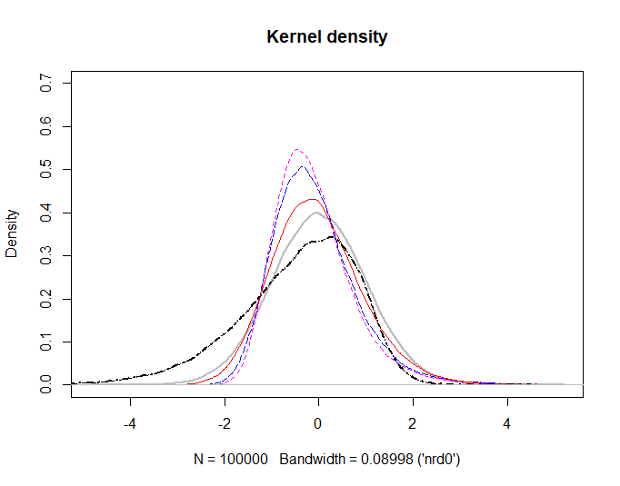
Figure 1: Kernel density functions for the statistics $Z_{\hat{\mathcal{L}}}$ and $S_{\hat{\mathcal{L}}}$ for the Theil index: Singh-Maddala distribution $SM(a_{0},b_{0},c_{0})$ with $(a_{0},c_{0})=(2.8,1.7)$ and $\zeta=4.76$. Gaussian density:    ; Statistic $Z_{\hat{\mathcal{L}}}$, $N=50$:        ; Statistic $Z_{\hat{\mathcal{L}}}$, $N=100$:       ; Statistic $Z_{\hat{\mathcal{L}}}$, $N=1000$:  ; Statistic $S_{\hat{\mathcal{L}}}$, $N=100$: ${\color[rgb]{0,0,0}\rule[2.5pt]{6.00006pt}{1.7pt}\ \mathbf{\cdot}\ \rule[2.5pt]{6.00006pt}{1.7pt}\ }$

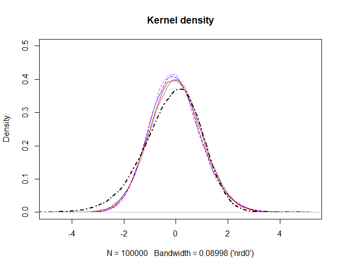
Figure 2: Kernel density functions for the statistics $Z_{\hat{\mathcal{L}}}$ and $S_{\hat{\mathcal{L}}}$ for the Gini index: Singh-Maddala distribution $SM(a,b_{0},c_{0})$ with $(a_{0},c_{0})=(2.8,1.7)$ and $\zeta=4.76.$ Gaussian density:    ; Statistic $Z_{\hat{\mathcal{L}}}$, $N=50$:        ; Statistic $Z_{\hat{\mathcal{L}}}$, $N=100$:       ; Statistic $Z_{\hat{\mathcal{L}}}$, $N=1000$:  ; Statistic $S_{\hat{\mathcal{L}}}$, $N=100$: ${\color[rgb]{0,0,0}\rule[2.5pt]{6.00006pt}{1.7pt}\ \mathbf{\cdot}\ \rule[2.5pt]{6.00006pt}{1.7pt}\ }$

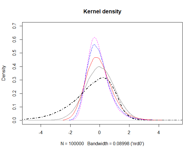
Figure 3: Kernel density functions for the statistics $Z_{\hat{\mathcal{L}}}$ and $S_{\hat{\mathcal{L}}}$ for the Gini index: Singh-Maddala distribution $SM(a,b_{0},c)$ with $(a,c)=(5.8,0.4473111)$ and $\zeta=2.59$. Gaussian density:   ; Statistic $Z_{\hat{\mathcal{L}}}$, $N=50$:        ; Statistic $Z_{\hat{\mathcal{L}}}$, $N=100$:       ; Statistic $Z_{\hat{\mathcal{L}}}$, $N=1000$:  ; Statistic $S_{\hat{\mathcal{L}}}$, $N=100$: ${\color[rgb]{0,0,0}\rule[2.5pt]{6.00006pt}{1.7pt}\ \mathbf{\cdot}\ \rule[2.5pt]{6.00006pt}{1.7pt}\ }$

3.1.2 Inference in one-sample problem: Finite-sample properties

Table 1 provides the results on the empirical size of asymptotic and the $t-$statistic robust tests on the Theil and Gini measures for sample sizes $N=200,500,1000$ and Singh-Maddala distributions $SM(a,b_{0},c)$ with the parameters $(a,c)=(2.5,2.502199),(3.2,1.2320215),(5.8,0.4996163)$ corresponding to the tail indices $\zeta=6.6,3.94,2.9$ in the case of the Theil index and the parameters $(a,c)=(2.5,2.640350),(3.2,1.1866026)$, and $(5.8,0.4473111)$ corresponding to $\zeta=6.26,3.8,2.9$ in the case of the Gini index.

In accordance with the above discussion of finite-sample distributions of statistics $Z$ and $S$ like those in Figures 1-3, the results in the table show that the finite-sample size of both the asymptotic and $t-$statistic robust tests becomes more distorted if the tail index decreases and thus the degree of heavy-tailedness in observations becomes more pronounced. Importantly, however, size distortions for the Gini measure are not so large as for the Theil measure. In the case of the number of groups $q=4$ or $q=8,$ the finite-sample size properties of robust tests based on $t-$statistics in group estimates are usually better than those of the tests based on asymptotic normality of the (full-sample) $t-$statistics for the measures. Further, the finite sample size properties of the robust $t-$statistic-based tests (with $q=4$) appear to be better than those of the asymptotic tests in the cases where each of the groups contains more than 100 observations, in accordance with the discussion of Figures 1-3.

Table 1: Empirical size: Identical distributions with $\zeta_{I}=\zeta_{Y}=\zeta$ and sample sizes $N_{1}=N_{2}=N$

Theil	$\zeta=6.26$	$\zeta=3.94$	$\zeta=2.9$	Gini	$\zeta=6.6$	$\zeta=3.8$	$\zeta=2.59$
$N=200$
asymptotic	8.2	14.5	25.5	asymptotic	6.2	7.5	13.0
$q=$4	6.9	10.6	18.0	$q=4$	5.2	5.2	7.7
$q=$8	11.0	17.8	28.7	$q=8$	5.2	6.0	11.3
$q=$12	15.9	24.9	37.3	$q=12$	5.5	6.6	14.2
$q=$16	21.3	33.1	45.9	$q=16$	5.5	6.9	16.9
$N=500$
asymptotic	6.9	11.9	20.2	asymptotic	5.7	6.5	10.8
$q=$4	5.8	8.2	13.5	$q=4$	4.8	5.1	7.1
$q=$8	8.3	12.9	20.6	$q=8$	5.3	5.9	9.5
$q=$12	10.0	16.2	25.6	$q=12$	5.1	6.3	11.5
$q=$16	12.7	20.0	30.0	$q=16$	5.1	6.4	13.0
$N=1000$
asymptotic	6.0	9.6	17.0	asymptotic	5.2	5.7	8.6
$q=$4	5.3	6.5	10.5	$q=4$	4.8	4.9	5.8
$q=$8	6.1	9.3	16.3	$q=8$	4.9	5.1	7.4
$q=$12	7.4	11.8	19.5	$q=12$	4.9	5.2	8.5
$q=$16	8.7	14.2	22.6	$q=16$	5.0	5.4	10.1

3.2 Two-sample problem: Testing equality of two inequality measures and inference on their difference

3.2.1 Inference in two-sample problem: Finite-sample distributions

In this section, we focus on comparisons of the finite-sample performance of the two-sample $t-$statistic robust inference approaches discussed in Section 2 with permutation and bootstrap tests proposed by Dufour et al. (2019).

In the numerical analysis in this section, $\mathcal{L}^{I}=\mathcal{L}(F_{1})$ and $\mathcal{L}^{Y}=\mathcal{L}(F_{2})$ denote the true values of the inequality measure $\mathcal{L}$ of interest (e.g., the Theil or Gini inequality index, as in the previous section) in two populations with cdf’s $F_{1}$ and $F_{2}$ considered. By $\hat{\mathcal{L}}^{I}=\hat{\mathcal{L}}^{I}(I_{1},...,I_{N_{1}})$ and $\hat{\mathcal{L}}^{Y}=\hat{\mathcal{L}}^{Y}(Y_{1},...,Y_{N_{2}})$ we denote the full-sample estimators of the measure $\mathcal{L}$ (the full-sample empirical inequality measures) calculated using samples of observations $I_{1},...,I_{N_{1}}$ and $Y_{1},...,Y_{N_{2}}$ from the two populations. Further, as in Section 2, by $\hat{\mathcal{L}}_{1}^{I},...,\hat{\mathcal{L}}_{q_{1}}^{I}$ and $\hat{\mathcal{L}}_{1}^{Y},...,\hat{\mathcal{L}}_{q_{2}}^{Y}$ we denote the group estimators of $\mathcal{L}$ (group empirical inequality measures) in the two samples dealt with in applications of $t-$statistic inference approaches.

Asymptotic approaches to testing the hypothesis $H_{0}:L_{1}-L_{2}=d_{0}$ (e.g., with $d_{0}=0,$ testing the hypothesis $H_{0}:L_{1}=L_{2}$ of equality of the values $L_{1},L_{2}$ of the measure $\mathcal{L}$ in the two populations considered) against the two-sided alternative $H_{a}:L_{1}-L_{2}\neq d_{0}$ (resp., with $d_{0}=0,$ against the two-sample alternative $H_{a}:L_{1}\neq L_{2}$) are based on the normal approximation to the sample distribution of the difference $\hat{\mathcal{L}}^{I}-\hat{\mathcal{L}}^{Y}$ between the full-sample estimators $\hat{\mathcal{L}}^{I}$ and $\hat{\mathcal{L}}^{Y}$ (full-sample empirical inequality measures). More precisely, the asymptotic approaches are based on the standard normal approximation to the sample distribution of the two-sample $t-$statistic $S_{\hat{\mathcal{L}}_{1}-\hat{\mathcal{L}}_{2}}=(\hat{\mathcal{L}}_{1}-\hat{\mathcal{L}}_{2}-d_{0})/s.e._{\hat{\mathcal{L}}_{1}-\hat{\mathcal{L}}_{2}}$ calculated using the estimators $\hat{\mathcal{L}}_{1}$ and $\hat{\mathcal{L}}_{2},$ where $s.e._{\hat{\mathcal{L}}_{1}-\hat{\mathcal{L}}_{2}}$ denotes the usual consistent standard error of the difference $\hat{\mathcal{L}}_{1}-\hat{\mathcal{L}}_{2}$ (see the formulas for the empirical inequality measures considered and the standard errors in Cowell and Flachaire, 2007, Davidson and Flachaire, 2007, Dufour et al., 2019).

Similar to the previous section, validity of two-sample $t-$statistic robust inference approaches based on (3) requires weak convergence of group estimators $\hat{\mathcal{L}}_{j}^{I},$ $j=1,...,q_{1},$ $\hat{\mathcal{L}}_{k}^{Y},$ $k=1,...,q_{2},$ of the inequality measure $\mathcal{L}$ in the two samples considered to possibly heterogeneous Gaussian distributions (or scale mixtures of Gaussian distributions). As discussed in the introduction and the previous section, asymptotic normality of group estimators $\hat{\mathcal{L}}_{j}^{I},$ $\hat{\mathcal{L}}_{k}^{Y},$ hold under the same conditions as in the case of the full-sample estimators $\hat{\mathcal{L}}^{I}$ and $\hat{\mathcal{L}}^{Y}.$ We refer to the previous section for the assessment of finite-sample distributions of the full-sample empirical inequality measures and their closeness to normality.

On the other hand, with $q_{1}=q_{2}=q,$ validity of the (two-sample) $t-$statistic robust inference approaches based on (4) - that is, the one-sample $t-$statistic $\tilde{\tilde{t}}_{\mathcal{L}}$ in the $q$ differences ${\widehat{\mathcal{L}}}^{I}_{j}-{\widehat{\mathcal{L}}}^{Y}_{j},$ $j=1,...,q,$ of the group empirical inequality measures $\hat{\mathcal{L}}_{j}^{I},$ $\hat{\mathcal{L}}_{j}^{Y}$ (without any Studentization/normalization of the differences between the group estimators by their standard errors in contrast to the $t-$statistics $S_{\hat{\mathcal{L}}_{1}-\hat{\mathcal{L}}_{2}}$ calculated using the full-sample estimators) requires weak convergence of the differences ${\widehat{\mathcal{L}}}^{I}_{j}-{\widehat{\mathcal{L}}}^{Y}_{j},$ $j=1,...,q,$ of the group estimators to possibly heterogeneous Gaussian distributions (or scale mixtures of Gaussian distributions). Further, asymptotic normality of the differences $\hat{\mathcal{L}}_{j}^{I}-\hat{\mathcal{L}}_{j}^{Y}$ between the group estimators holds under the same conditions as in the case of the difference $\hat{\mathcal{L}}^{I}-\hat{\mathcal{L}}^{Y}$ between the full-sample estimators.

We, therefore, begin the analysis with an assessment of finite-sample distributions of the difference $\hat{\mathcal{L}}^{I}-\hat{\mathcal{L}}^{Y}$ between the (full-sample) empirical inequality measures $\hat{\mathcal{L}}^{I},$ $\hat{\mathcal{L}}^{Y}$ and of the (full-sample) $t-$statistics $S_{\hat{\mathcal{L}}^{I}-\hat{\mathcal{L}}^{Y}}$ calculated using them. We, in particular, focus on the assessment of closeness of the above finite-sample distributions to Gaussian ones.

We focus on comparisons of finite-sample distributions of the $t-$statistic $S_{\hat{\mathcal{L}}^{I}-\hat{\mathcal{L}}^{Y}}$ with those of the difference $\hat{\mathcal{L}}^{I}-\hat{\mathcal{L}}^{Y}$ normalized by its true standard deviation, that is, of the statistic $Z_{\hat{\mathcal{L}}^{I}-\hat{\mathcal{L}}^{Y}}=(\hat{\mathcal{L}}^{I}-\hat{\mathcal{L}}^{Y})/\sigma_{\hat{\mathcal{L}}^{I}-\hat{\mathcal{L}}^{Y}},$ where $\sigma^{2}_{\hat{\mathcal{L}}^{I}-\hat{\mathcal{L}}^{Y}}=Var(\hat{\mathcal{L}}^{I}-\hat{\mathcal{L}}^{Y}).$

In Figures 4-6, we present kernel estimates of the finite-sample densities of the statistics $Z_{\hat{\mathcal{L}}^{I}-\hat{\mathcal{L}}^{Y}}$ and $S_{\hat{\mathcal{L}}^{I}-\hat{\mathcal{L}}^{Y}}$ for the difference between the empirical inequality measures in two samples from populations with the same Singh-Maddala distribution.

Figures 4-5 provide kernel density functions, for sample sizes $N_{1}=N_{2}=N,$ of the statistics $Z_{\hat{\mathcal{L}}^{I}-\hat{\mathcal{L}}^{Y}}$ ($N=50,100,1000$) and $S_{\hat{\mathcal{L}}^{I}-\hat{\mathcal{L}}^{Y}}$ (sample sizes $N=100$) for the difference between, respectively, the Theil and Gini empirical inequality measures in two samples from the Singh-Maddala distribution $SM(a_{0},b_{0},c_{0})$ with the parameters $a_{0}=2.8,$ $b_{0}=100^{-1/2.8},$ $c_{0}=1.7$ and the corresponding tail index $\zeta=4.76.$ Figure 6 provides the above kernel density functions for the Gini index in the case of two samples from a more heavy-tailed Singh-Maddala distribiion $SM(a,b_{0},c)$ with $(a,c)=(5.8,0.4473111)$ and the tail index $\zeta=2.59.$

According to Figures 4-6, the finite-sample distributions of the statistic $Z_{\hat{\mathcal{L}}^{I}-\hat{\mathcal{L}}^{Y}}$ and thus of the difference $\hat{\mathcal{L}}^{I}-\hat{\mathcal{L}}^{Y}$ between the estimators of the Theil and Gini measures is approximately symmetric even in rather small samples and also under pronounced heavy-tailedness, with good performance of Gaussian approximations, e.g., as compared to finite-sample distribution of the (full-sample) $t-$statistic $S_{\hat{\mathcal{L}}^{I}-\hat{\mathcal{L}}^{Y}}.$ This also holds in the case when the sample sizes are not very different.

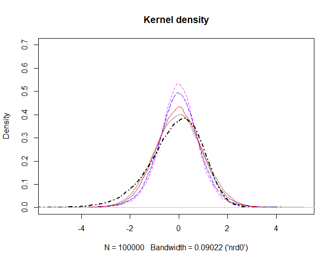
Figure 4: Kernel density functions for the statistics $Z_{\hat{\mathcal{L}}^{I}-\hat{\mathcal{L}}^{Y}}$ and $S_{\hat{\mathcal{L}}^{I}-\hat{\mathcal{L}}^{Y}}$ for the difference between Theil indices: Singh-Maddala distributions $SM(a_{0},b_{0},c_{0})$ with $(a_{0},c_{0})=(2.8,1.7)$ and $\zeta=4.76.$ Gaussian density:   ; Statistic $Z_{\hat{\mathcal{L}}^{I}-\hat{\mathcal{L}}^{Y}}$, $N=50$:        ; Statistic $Z_{\hat{\mathcal{L}}^{I}-\hat{\mathcal{L}}^{Y}}$, $N=100$:       ; Statistic $Z_{\hat{\mathcal{L}}^{I}-\hat{\mathcal{L}}^{Y}}$, $N=1000$:  ; Statistic $S_{\hat{\mathcal{L}}^{I}-\hat{\mathcal{L}}^{Y}}$, $N=100$: ${\color[rgb]{0,0,0}\rule[2.5pt]{6.00006pt}{1.7pt}\ \mathbf{\cdot}\ \rule[2.5pt]{6.00006pt}{1.7pt}\ }$

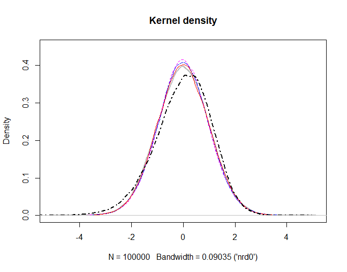
Figure 5: Kernel density functions for the statistics $Z_{\hat{\mathcal{L}}^{I}-\hat{\mathcal{L}}^{Y}}$ and $S_{\hat{\mathcal{L}}^{I}-\hat{\mathcal{L}}^{Y}}$ for the difference between Gini indices: Singh-Maddala distributions $SM(a_{0},b_{0},c_{0})$ with $(a_{0},c_{0})=(2.8,1.7)$ and $\zeta=4.76.$. Gaussian density:   ; Statistic $Z_{\hat{\mathcal{L}}^{I}-\hat{\mathcal{L}}^{Y}}$, $N=50$:        ; Statistic $Z_{\hat{\mathcal{L}}^{I}-\hat{\mathcal{L}}^{Y}}$, $N=100$:       ; Statistic $Z_{\hat{\mathcal{L}}^{I}-\hat{\mathcal{L}}^{Y}}$, $N=1000$:  , Statistic $S_{\hat{\mathcal{L}}^{I}-\hat{\mathcal{L}}^{Y}}$, $N=100$: ${\color[rgb]{0,0,0}\rule[2.5pt]{6.00006pt}{1.7pt}\ \mathbf{\cdot}\ \rule[2.5pt]{6.00006pt}{1.7pt}\ }$

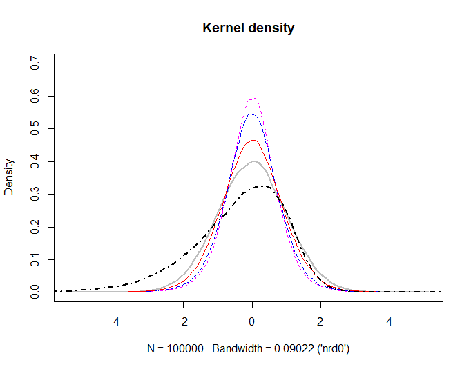
Figure 6: Kernel density functions for the statistics $Z_{\hat{\mathcal{L}}^{I}-\hat{\mathcal{L}}^{Y}}$ and $S_{\hat{\mathcal{L}}^{I}-\hat{\mathcal{L}}^{Y}}$ for the difference between Gini indices: Singh-Maddala distributions $SM(a,b_{0},c)$ with $(a,c)=(5.8,0.4473111)$ and $\zeta=2.59.$ Gaussian density:   ; Statistic $Z_{\hat{\mathcal{L}}^{I}-\hat{\mathcal{L}}^{Y}}$, $N=50$:        ; Statistic $Z_{\hat{\mathcal{L}}^{I}-\hat{\mathcal{L}}^{Y}}$, $N=100$:       ; Statistic $Z_{\hat{\mathcal{L}}^{I}-\hat{\mathcal{L}}^{Y}}$, $N=1000$:  ; Statistic $S_{\hat{\mathcal{L}}^{I}-\hat{\mathcal{L}}^{Y}},$ $N=100$: ${\color[rgb]{0,0,0}\rule[2.5pt]{6.00006pt}{1.7pt}\ \mathbf{\cdot}\ \rule[2.5pt]{6.00006pt}{1.7pt}\ }$

3.2.2 Inference in two-sample problem: Finite-sample size properties

Tables 2-7 provide the results on the finite-sample size properties of the asymptotic, permutation, bootstrap and $t-$statistic robust tests on equality of Theil and Gini measures. As before, we consider two samples $I_{1},...,I_{N_{1}}$ and $Y_{1},...,Y_{N_{2}}$ from, respectively, Singh-Maddala distributions $SM(a_{I},b_{0},c_{I})$ and $SM(a_{Y},b_{0},c_{Y}),$ with $b_{0}=100^{-1/2.8}$ and the tail indices $\zeta_{I}=a_{I}c_{I},$ $\zeta_{Y}=a_{Y}c_{Y}.$ In simulations, we consider the following settings with identical/different sample sizes $N_{1},$ $N_{2};$ distributions $S(a_{I},b_{0},c_{I})$ and $S(a_{Y},b_{0},c_{Y})$ in the samples and the number $q_{1},q_{2}$ of groups used in $t-$statistic robust tests.

Tables 2-6 provide the results on finite-sample size properties of asymptotic, permutation, bootstrap and $t-$statistic robust tests based on (3) and (4) with the equal number of groups $q_{1}=q_{2}=q.$

1. Identical distributions and sample sizes $N_{1}=N_{2}=N=200$ (Table 2).

   The values of the parameters $(a,c)$ as in Dufour et al. (2019) and Table 2: $(a_{I},c_{I})=(a_{Y},c_{Y})=(2.5,2.502199),(3.2,1.2320215),(5.8,0.4996163)$ and $\zeta_{I}=\zeta_{Y}=\zeta=6.6,3.94,2.9$ (Theil index); $(a_{I},c_{I})=(a_{Y},c_{Y})=(2.5,2.640350),(3.2,1.1866026),(5.8,0.4473111)$ and $\zeta_{I}=\zeta_{Y}=\zeta=6.6,3.8,2.59$ (Gini index);

   Singh-Maddala distributions with tail indices $\zeta$ similar to the empirical results in the literature with $\zeta\in(1.5,3)$ for income and $\zeta\approx 1.5$ for wealth (see Section 3 and references therein):

   $(a_{I},c_{I})=(a_{Y},c_{Y})=(2,1.1)$ and $\zeta_{I}=\zeta_{Y}=\zeta=2.2;$ $(a_{I},c_{I})=(a_{Y},c_{Y})=(2,0.7)$ and $\zeta_{I}=\zeta_{Y}=\zeta=1.4$ (Theil and Gini measures).

The results in Table 2 indicate that the size of all the tests, except the asymptotic ones, never exceeds the nominal 5% level. In addition, in a number of cases, it is quite close to the nominal level for the permutation, bootstrap and the robust $t-$statistic tests.

1. Identical sample sizes $N_{1}=N_{2}=N=200$ and different distributions (Table 3).

   $(a_{I},c_{I})=(2.8,1.7)$ and $\zeta_{I}=4.76;$

   $(a_{Y},c_{Y})$=$(2.5,2.502199),(3.2,1.2320215),(5.8,0.4996163);$ $\zeta_{Y}=2.9,3.94,6.6$ (Theil index);

   $(a_{Y},c_{Y})$=$(2.5,2.640350),(3.2,1.1866026),(5.8,0.4473111);$ $\zeta_{Y}=2.9,3.8,6.26$ (Gini index).

According to Table 3, the empirical sizes of the robust two-sample $t-$statistic tests based on (3) with $q=4,8$ in the case of more heavy-tailed distributions and on (4) with $q=4,8,12,16$ in the case of less heavy-tailed distributions are comparable and in some cases are better than those of the permutation and bootstrap tests. Comparing the robust tests based on the two-sample $t-$statistic (3) in group estimators and those based on the one-sample $t-$statistic (4) in the differences of the group estimators, overall, the former tests with the same number of groups $q_{1}=q_{2}=q$ appear to have less over-rejections as compared to the latter ones.

1. Different sample sizes $N_{1},N_{2}$ and identical distributions (Tables 4 and 5).

   $N_{1}=200,$ $N_{2}=50,200,500,1000,5000;$

   $(a_{I},c_{I})=(a_{Y},c_{Y})=(5.8,0.4996163)$ and $\zeta_{I}=\zeta_{Y}=2.9$ in the case of the Theil index; $(a_{I},c_{I})=(a_{Y},c_{Y})=(5.8,0.4473111)$ and $\zeta_{I}=\zeta_{Y}=2.59$ in the case of the Gini index (Table 4);

   $(a_{I},c_{I})=(a_{Y},c_{Y})=(2,0.7)$ and $\zeta_{I}=\zeta_{Y}=1.4$ (Theil and Gini measures, Table 5).

The finite-sample size of all the tests, except the asymptotic ones, appears to be good in all parameter settings: e.g., essentially no over-rejections are observed for $t-$statistic inference approaches, including the settings with more pronounced heavy-tailedness and infinite variances in Table 5. Further, the finite sample properties of the robust $t-$statistic approaches are comparable or similar and in some cases are better than those of the bootstrap and permutation approaches. Importantly, asymptotic normality of sample Theil and Gini measures is lost under infinite variances, as is the case for tail indices $\zeta_{I}=\zeta_{Y}=1.4$ in Table 5 (see Fontanari et al. (2018) and the discussion in Appendix B). However, according to the results in the table, the $t-$statistic approaches have good finite sample size properties even in such heavy-tailed settings. This is due to robustness of $t-$statistic approaches to heavy-tailedness as they may be used under convergence of group estimators of parameters in consideration to scale mixtures of normals.

1. Different sample sizes $N_{1},N_{2}$ and different distributions (Table 6).

   $N_{1}=200,$ $N_{2}=50,200,500,1000,5000;$

   $(a_{I},c_{I})=(2.8,1.7)$ and $\zeta_{I}=4.76;$

   $(a_{Y},c_{Y})=(5.8,0.4996163)$ and $\zeta_{Y}=2.9$ (Theil index); $(a_{Y},c_{Y})=(5.8,0.4473111)$ and $\zeta_{Y}=2.59$ (Gini index).

In Table 6, one can observe better size properties for two-sample $t-$statistic inference approaches based on $\tilde{t}_{\mathcal{L}}$ in (3) (with $q_{1}=q_{2}=4,8,12$ for all sample sizes and also $q=16$ for large sample sizes) and those based on $\tilde{\tilde{t}}_{\mathcal{L}}$ in (4) (with $q_{1}=q_{2}=4,8$ for all sample sizes) in comparison to permutation and bootstrap tests.

Table 2: Empirical size, identical distributions with $\zeta_{I}=\zeta_{Y}=\zeta$ and sample sizes $N_{1}=N_{2}=200$

Theil \$\zeta$	6.26	3.94	2.9	2.2	1.4	Gini\$\zeta$	6.6	3.8	2.59	2.2	1.4
asymptotic	5.4	5.5	5.3	7.6	22.1	asy	5.7	6.1	7.0	8.4	18.8
$\tilde{t}_{\mathcal{L}}(q=4)$	2.0	1.7	1.5	1.5	1.3	$\tilde{t}_{\mathcal{L}}(q=4)$	2.1	1.9	1.9	2.0	2.0
$\tilde{t}_{\mathcal{L}}(q=8)$	3.2	2.7	2.2	2.4	2.4	$\tilde{t}_{\mathcal{L}}(q=8)$	3.5	3.4	3.0	3.2	3.4
$\tilde{t}_{\mathcal{L}}(q=12)$	3.6	3.2	2.7	2.9	3.0	$\tilde{t}_{\mathcal{L}}(q=12)$	3.8	3.7	3.4	3.7	3.7
$\tilde{t}_{\mathcal{L}}(q=16)$	4.0	3.7	3.1	3.4	3.5	$\tilde{t}_{\mathcal{L}}(q=16)$	4.4	4.2	4.1	4.0	4.1
$\tilde{\tilde{t}}_{\mathcal{L}}(q=4)$	4.6	4.4	3.5	3.5	2.9	$\tilde{\tilde{t}}_{\mathcal{L}}(q=4)$	5.0	4.9	4.4	4.6	4.6
$\tilde{\tilde{t}}_{\mathcal{L}}(q=8)$	4.7	4.1	3.3	3.7	3.7	$\tilde{\tilde{t}}_{\mathcal{L}}(q=8)$	4.9	4.8	4.5	4.9	4.9
$\tilde{\tilde{t}}_{\mathcal{L}}(q=12)$	4.9	4.3	3.5	3.8	4.1	$\tilde{\tilde{t}}_{\mathcal{L}}(q=12)$	5.1	4.9	4.6	4.8	4.9
$\tilde{\tilde{t}}_{\mathcal{L}}(q=16)$	5.0	4.5	3.8	4.1	4.3	$\tilde{\tilde{t}}_{\mathcal{L}}(q=16)$	5.3	5.1	4.7	4.8	5.0
permutation	4.8	4.7	4.9	4.7	4.7	permutation	4.4	4.5	4.8	4.8	4.5
bootstrap	4.5	4.2	3.4	3.3	2.8	bootstrap	4.8	4.4	4.1	3.9	3.9

Table 3: Empirical size, identical sample sizes $N_{1}=N_{2}=200$ and different distributions, $\zeta_{I}=4.76$

Theil\$\zeta_{Y}$	6.26	3.94	2.9	Gini \$\zeta_{Y}$	6.6	3.8	2.59
asy	5.1	5.4	12.3	asy	5.2	5.5	8.0
$\tilde{t}_{\mathcal{L}}(q=4)$	1.9	1.5	4.0	$\tilde{t}_{\mathcal{L}}(q=4)$	1.9	1.7	2.7
$\tilde{t}_{\mathcal{L}}(q=8)$	3.1	2.9	8.7	$\tilde{t}_{\mathcal{L}}(q=8)$	3.2	3.1	5.1
$\tilde{t}_{\mathcal{L}}(q=12)$	3.6	3.4	11.4	$\tilde{t}_{\mathcal{L}}(q=12)$	3.8	3.6	6.6
$\tilde{t}_{\mathcal{L}}(q=16)$	4.0	3.9	13.6	$\tilde{t}_{\mathcal{L}}(q=16)$	3.9	3.9	7.8
$\tilde{\tilde{t}}_{\mathcal{L}}(q=4)$	4.8	4.3	7.2	$\tilde{\tilde{t}}_{\mathcal{L}}(q=4)$	5.1	4.7	5.7
$\tilde{\tilde{t}}_{\mathcal{L}}(q=8)$	5.0	4.5	10.6	$\tilde{\tilde{t}}_{\mathcal{L}}(q=8)$	5.1	4.8	6.6
$\tilde{\tilde{t}}_{\mathcal{L}}(q=12)$	4.8	4.6	12.6	$\tilde{\tilde{t}}_{\mathcal{L}}(q=12)$	5.0	4.8	8.1
$\tilde{\tilde{t}}_{\mathcal{L}}(q=16)$	5.1	4.8	14.5	$\tilde{\tilde{t}}_{\mathcal{L}}(q=16)$	5.0	4.8	8.8
permutation	4.8	4.8	11.0	permutation	4.4	4.6	6.2
bootstrap	4.8	4.7	10.6	bootstrap	4.6	4.4	6.3

Table 4: Empirical size, identical distributions with $\zeta_{I}=\zeta_{Y}=\zeta$ and different sample sizes, $N_{1}=200$

Theil, $\zeta=2.9$ \$N_{2}$	50	200	500	1000	5000	Gini, $\zeta=2.59$\$N_{2}$	50	200	500	1000	5000
asymptotic	8.7	5.3	4.7	4.6	4.5	asy	12.3	6.6	5.7	5.4	5.2
$\tilde{t}_{\mathcal{L}}(q=4)$	1.2	1.2	1.6	1.5	1.6	$\tilde{t}_{\mathcal{L}}(q=4)$	1.5	1.5	1.8	1.8	1.7
$\tilde{t}_{\mathcal{L}}(q=8)$	2.2	2.0	2.4	2.4	2.5	$\tilde{t}_{\mathcal{L}}(q=8)$	3.1	2.7	3.2	3.1	3.4
$\tilde{t}_{\mathcal{L}}(q=12)$	2.7	2.4	2.9	2.8	3.0	$\tilde{t}_{\mathcal{L}}(q=12)$	3.6	3.4	3.5	3.6	4.0
$\tilde{t}_{\mathcal{L}}(q=16)$	3.5	2.8	3.2	3.3	3.4	$\tilde{t}_{\mathcal{L}}(q=16)$	4.3	3.7	3.6	3.9	4.2
$\tilde{\tilde{t}}_{\mathcal{L}}(q=4)$	2.9	3.1	3.7	3.7	3.7	$\tilde{\tilde{t}}_{\mathcal{L}}(q=4)$	4.3	4.4	4.8	4.7	4.8
$\tilde{\tilde{t}}_{\mathcal{L}}(q=8)$	3.6	3.2	3.9	3.7	4.0	$\tilde{\tilde{t}}_{\mathcal{L}}(q=8)$	4.5	4.4	4.8	4.7	4.6
$\tilde{\tilde{t}}_{\mathcal{L}}(q=12)$	3.8	3.7	3.8	3.7	4.4	$\tilde{\tilde{t}}_{\mathcal{L}}(q=12)$	4.9	4.6	4.7	4.9	5.1
$\tilde{\tilde{t}}_{\mathcal{L}}(q=16)$	4.5	3.5	3.8	3.9	4.0	$\tilde{\tilde{t}}_{\mathcal{L}}(q=16)$	5.2	4.6	4.7	4.7	4.8
permutation	5.0	4.8	4.9	4.9	5.0	permutation	5.1	4.9	5.0	4.9	5.2
bootstrap	4.0	4.2	4.1	4.5	4.7	bootstrap	4.6	4.8	4.8	5.1	5.3

Table 5: Empirical size, identical distributions with $\zeta_{I}=\zeta_{Y}=1.4$ and different sample sizes, $N_{1}=200$

Theil\$N_{2}$	50	200	500	1000	5000	Gini \$N_{2}$	50	200	500	1000	5000
asymptotic	31.5	21.9	16.7	13.8	8.7	asymptotic	28.9	18.3	14.0	12.3	8.6
$\tilde{t}_{\mathcal{L}}(q=4)$	1.0	1.1	1.3	1.1	1.1	$\tilde{t}_{\mathcal{L}}(q=4)$	1.7	1.7	1.9	1.6	1.6
$\tilde{t}_{\mathcal{L}}(q=8)$	2.5	2.2	2.3	2.1	2.0	$\tilde{t}_{\mathcal{L}}(q=8)$	3.3	3.0	3.1	3.2	2.7
$\tilde{t}_{\mathcal{L}}(q=12)$	3.5	3.0	3.1	2.9	2.7	$\tilde{t}_{\mathcal{L}}(q=12)$	3.8	3.5	3.8	3.7	3.5
$\tilde{t}_{\mathcal{L}}(q=16)$	4.0	3.3	3.3	3.5	3.0	$\tilde{t}_{\mathcal{L}}(q=16)$	4.3	3.8	4.1	4.0	4.0
$\tilde{\tilde{t}}_{\mathcal{L}}(q=4)$	3.0	3.0	3.1	2.8	2.7	$\tilde{\tilde{t}}_{\mathcal{L}}(q=4)$	4.7	4.5	4.5	4.3	3.9
$\tilde{\tilde{t}}_{\mathcal{L}}(q=8)$	4.0	3.5	3.6	3.5	3.2	$\tilde{\tilde{t}}_{\mathcal{L}}(q=8)$	5.2	4.8	4.9	4.7	4.3
$\tilde{\tilde{t}}_{\mathcal{L}}(q=12)$	4.7	4.1	3.9	3.8	3.7	$\tilde{\tilde{t}}_{\mathcal{L}}(q=12)$	5.1	5.0	4.9	4.9	4.8
$\tilde{\tilde{t}}_{\mathcal{L}}(q=16)$	5.2	4.2	4.1	4.2	3.7	$\tilde{\tilde{t}}_{\mathcal{L}}(q=16)$	5.4	4.9	4.7	5.0	4.6
permutation	4.9	4.8	5.1	5.1	4.9	permutation	5.1	4.7	4.9	5.0	5.0
bootstrap	3.3	3.4	3.6	3.6	3.6	bootstrap	4.5	4.2	4.3	4.4	4.1

Table 6: Empirical size, different distributions and sample sizes, $\zeta_{I}=4.76,$ $N_{1}=200$

Theil, $\zeta_{Y}=2.9$ \$N_{2}$	50	200	500	1000	5000	Gini, $\zeta_{Y}=2.59$\$N_{2}$	50	200	500	1000	5000
asymptotic	14.5	12.3	12.2	11.2	9.0	asymptotic	12.6	8.0	7.5	6.6	6.0
$\tilde{t}_{\mathcal{L}}(q=4)$	3.9	4.0	4.8	4.2	4.0	$\tilde{t}_{\mathcal{L}}(q=4)$	2.8	2.7	2.9	2.7	2.6
$\tilde{t}_{\mathcal{L}}(q=8)$	8.8	8.7	8.6	8.0	6.7	$\tilde{t}_{\mathcal{L}}(q=8)$	6.0	5.1	5.1	4.8	4.3
$\tilde{t}_{\mathcal{L}}(q=12)$	11.4	11.4	11.3	9.7	7.8	$\tilde{t}_{\mathcal{L}}(q=12)$	7.7	6.6	6.6	5.8	5.1
$\tilde{t}_{\mathcal{L}}(q=16)$	13.9	13.6	12.8	11.2	8.4	$\tilde{t}_{\mathcal{L}}(q=16)$	9.8	7.8	7.5	6.6	5.5
$\tilde{\tilde{t}}_{\mathcal{L}}(q=4)$	6.9	7.2	7.8	7.3	6.6	$\tilde{\tilde{t}}_{\mathcal{L}}(q=4)$	5.7	5.7	6.1	5.7	5.2
$\tilde{\tilde{t}}_{\mathcal{L}}(q=8)$	11.1	10.6	10.2	9.6	7.9	$\tilde{\tilde{t}}_{\mathcal{L}}(q=8)$	8.2	6.6	6.8	6.2	5.6
$\tilde{\tilde{t}}_{\mathcal{L}}(q=12)$	13.0	12.6	12.2	10.9	8.7	$\tilde{\tilde{t}}_{\mathcal{L}}(q=12)$	9.3	8.1	7.7	6.9	6.2
$\tilde{\tilde{t}}_{\mathcal{L}}(q=16)$	14.9	14.5	13.6	12.1	9.0	$\tilde{\tilde{t}}_{\mathcal{L}}(q=16)$	11.0	8.8	8.2	7.4	6.2
permutation	12.4	11.0	11.6	10.5	8.8	permutation	8.9	6.2	6.5	6.1	5.6
bootstrap	12.2	10.6	11.1	10.4	8.5	bootstrap	9.1	6.3	6.3	6.0	5.7

Table 7 is an analogue of Tables 4 and 5 with different numbers $q_{1},q_{2}$ of groups used in two-sample $t-$statistic robust inference approaches based on $\tilde{t}_{\mathcal{L}}$ in (3). It provides the results on the empirical size of the tests based on these approaches with asymptotic, bootstrap and permutation tests in the following settings.

1. Identical distributions and different sample sizes $N_{1},N_{2}$ and the numbers $q_{1},q_{2}$ of groups

   $(a_{I},c_{I})=(a_{Y},c_{Y})=(2,1.1),$ $\zeta_{I}=\zeta_{Y}=2.2;$

   $N_{1}=200,$ $N_{2}=400,600,800.$

According to the results in Table 7, in the case of two-sample $t-$statistic inference on equality of/the difference between Theil indices, only the choice of $q_{1}=q_{2}=4$ leads to size control for all sample sizes considered. Size distortion of the $t-$statistic approaches in the case of Theil indices is apparently due to skewness in finite-sample distributions of (group) empirical Theil inequality measures implying poor quality of normal approximations to them (see Section 3.1.1). The solution may be to use different number of groups $q_{1},q_{2}$ for different sample size pairs $N_{1},N_{2}$. E.g., according to Table 7, in the case of inference on equality/the difference between the Theil indices, good size properties of two-sample $t-$statistic approaches are observed with $(q_{1},q_{2})=(8,8)$ for $N_{1}=200,N_{2}=400$, $(q_{1},q_{2})=(6,8)$ for $N_{1}=200,N_{2}=600$ and $(q_{1},q_{2})=(6,12)$ for $N_{1}=200,N_{2}=800$. The finite-sample distributions of (group) empirical Gini measures are not so skewed and better approximated by normal ones as compared to the Theil measures (see Section 3.1.1). In Table 7, one observes good size control for different combinations of $q_{1}$ and $q_{2}$ in $t-$statistic robust tests of equality of/the difference between the Gini indices except only the cases $q_{1}=q_{2}=12$, $q_{1}=q_{2}=16$ and $q_{1}=12,q_{2}=16$ with rather small number of observations in each of the group. To avoid very conservative size properties, the best choices for the number of groups in applications of $t-$statistic robust tests in the case of Gini indices appear to be $(q_{1},q_{2})=(8,8)$, $(q_{1},q_{2})=(9,12)$ and $(q_{1},q_{2})=(8,16)$ for all sample sizes $N_{1},N_{2}$ considered.

Table 7: Empirical size, identical distributions with $\zeta_{I}=\zeta_{Y}=2.2$ and different sample sizes, $N_{1}=200$

Theil \$N_{2}$	400	600	800	Gini\$N_{2}$	400	600	800
asymptotic	8.8	9.3	11.4	asymptotic	8.8	8.1	9.1
$\tilde{t}_{\mathcal{L}}(q_{1}=4,q_{2}=4)$	1.9	2.3	3.2	$\tilde{t}_{\mathcal{L}}(q_{1}=4,q_{2}=4)$	2.2	2.1	2.7
$\tilde{t}_{\mathcal{L}}(q_{1}=8,q_{2}=8)$	4.2	6.3	8.6	$\tilde{t}_{\mathcal{L}}(q_{1}=8,q_{2}=8)$	3.9	4.3	5.1
$\tilde{t}_{\mathcal{L}}(q_{1}=12,q_{2}=12)$	6.8	11.1	15.1	$\tilde{t}_{\mathcal{L}}(q_{1}=12,q_{2}=12)$	5.1	5.7	6.8
$\tilde{t}_{\mathcal{L}}(q_{1}=16,q_{2}=16)$	9.4	15.9	21.6	$\tilde{t}_{\mathcal{L}}(q_{1}=16,q_{2}=16)$	5.8	6.6	8.7
$\tilde{t}_{\mathcal{L}}(q_{1}=3,q_{2}=4)$	0.7	0.7	1.1	$\tilde{t}_{\mathcal{L}}(q_{1}=3,q_{2}=4)$	0.8	1.0	1.3
$\tilde{t}_{\mathcal{L}}(q_{1}=6,q_{2}=8)$	2.5	3.6	5.5	$\tilde{t}_{\mathcal{L}}(q_{1}=6,q_{2}=8)$	2.8	3.1	3.8
$\tilde{t}_{\mathcal{L}}(q_{1}=9,q_{2}=12)$	4.1	6.3	9.4	$\tilde{t}_{\mathcal{L}}(q_{1}=9,q_{2}=12)$	3.9	4.1	5.0
$\tilde{t}_{\mathcal{L}}(q_{1}=12,q_{2}=16)$	6.0	9.5	14.0	$\tilde{t}_{\mathcal{L}}(q_{1}=12,q_{2}=16)$	4.8	5.1	6.4
$\tilde{t}_{\mathcal{L}}(q_{1}=2,q_{2}=4)$	0.1	0.1	0.1	$\tilde{t}_{\mathcal{L}}(q_{1}=2,q_{2}=4)$	0.0	0.1	0.1
$\tilde{t}_{\mathcal{L}}(q_{1}=4,q_{2}=8)$	1.1	1.1	1.9	$\tilde{t}_{\mathcal{L}}(q_{1}=4,q_{2}=8)$	1.4	1.5	2.0
$\tilde{t}_{\mathcal{L}}(q_{1}=6,q_{2}=12)$	2.1	2.9	4.6	$\tilde{t}_{\mathcal{L}}(q_{1}=6,q_{2}=12)$	2.6	2.8	3.4
$\tilde{t}_{\mathcal{L}}(q_{1}=8,q_{2}=168)$	3.1	4.5	6.9	$\tilde{t}_{\mathcal{L}}(q_{1}=8,q_{2}=16)$	3.4	3.6	4.5
permutation	5.4	4.9	4.9	permutation	5.4	4.7	4.8
bootstrap	4.6	3.7	4.0	bootstrap	5.3	4.4	4.4

Finally, Table 8 provides the results for the case of samples with dependent observations, i.e., those with spatially dependent data relevant for studies of income distributions and inequality. Each of the two samples consists of 192 observations with the standard (parameters $\mu=0$ and $\sigma=1$) lognormal distribution located on a rectangular array of unit squares with 16 rows and 12 columns. The observations are generated such that the correlation between the logarithms of two observations is given by $\exp(-\phi d)$ for some $\phi>0,$ where $d$ is the Euclidean distance between the two observations (see Section 3.4 in Ibragimov and Müller (2010) for the use of a similar spatially correlated setting in the analysis of finite sample size properties of one-sample $t-$statistic approaches in inference on the mean of Gaussian observations with spatial dependence). The case $\phi=\infty$ to samples of i.i.d. observations.

More precisely, the observations in the samples are given by $I_{ij}=\exp(u_{ij}),$ $Y_{ij}=\exp(v_{ij}),$ $i=1,...,16,$ $j=1,...,12,$ where $u_{ij}$ and $v_{ij}$ are multivariate mean zero unit variance Gaussian with correlation between $u_{ij}$ and $u_{lk}$ and between $v_{ij}$ and $v_{lk}$ equals $\exp(-\phi\sqrt{(i-l)^{2}+(j-k)^{2}}).$

According to the results in Table 8, the empirical size properties of $t-$statistic tests of equality of Theil and Gini indices in the two samples with spatial dependence are comparable (especially, for the tests based on the two-sample $t-$statistic $\tilde{\tilde{t}}$ with $q_{1}=q_{2}=q=4$ groups and the one-sample $t-$statistic $\tilde{t}$ in differences with $q=8$) to those of permutation and bootstrap procedures. Furthermore, the finite sample size properties of essentially all robust $t-$statistic tests are better than those of bootstrap and permutation tests under pronounced spatial dependence with $\phi=1.$

Table 8: Empirical size, spatial correlation

Theil \$\phi$	$\infty$	2	1	Gini\$\phi$	$\infty$	2	1
asymptotic	7.1	7.6	14.6	asymptotic	7.4	7.9	16.3
$\tilde{t}_{\mathcal{L}}(q=4)$	1.6	1.6	2.0	$\tilde{t}_{\mathcal{L}}(q=4)$	1.6	1.6	2.0
$\tilde{t}_{\mathcal{L}}(q=8)$	5.4	5.3	6.0	$\tilde{t}_{\mathcal{L}}(q=8)$	5.4	5.3	6.0
$\tilde{t}_{\mathcal{L}}(q=12)$	6.8	7.3	8.1	$\tilde{t}_{\mathcal{L}}(q=12)$	6.8	7.3	8.1
$\tilde{t}_{\mathcal{L}}(q=16)$	7.5	7.8	8.7	$\tilde{t}_{\mathcal{L}}(q=16)$	7.5	7.8	8.7
$\tilde{\tilde{t}}_{\mathcal{L}}(q=4)$	4.2	4.3	4.7	$\tilde{\tilde{t}}_{\mathcal{L}}(q=4)$	4.2	4.3	4.7
$\tilde{\tilde{t}}_{\mathcal{L}}(q=8)$	7.1	7.4	8.1	$\tilde{\tilde{t}}_{\mathcal{L}}(q=8)$	7.1	7.4	8.1
$\tilde{\tilde{t}}_{\mathcal{L}}(q=12)$	8.2	8.6	9.7	$\tilde{\tilde{t}}_{\mathcal{L}}(q=12)$	8.2	8.6	9.7
$\tilde{\tilde{t}}_{\mathcal{L}}(q=16)$	8.7	9.0	9.8	$\tilde{\tilde{t}}_{\mathcal{L}}(q=16)$	8.7	9.0	9.8
permutation	4.4	4.8	10.1	permutation	4.1	4.3	9.3
bootstrap	4.4	4.9	11.2	bootstrap	4.3	4.9	11.0

3.2.3 Inference in two-sample problem: Finite-sample power properties

Next, we investigate finite-sample power properties of the tests considered. We report finite-sample size adjusted power for two-sample $t-$statistic and permutation tests.. Under size adjustment, the resulting empirical size of a given $t$-statistic-based robust test and its permutation counterpart coincide under the null hypothesis, thereby enabling meaningful power comparisons.

We consider the following simulation designs.

Table 9 presents the size-adjusted power when the two samples come from different Singh-Maddala distributions $SM(a_{0},b_{0},c).$ The sample sizes are $N_{1}=N_{2}=200,$ and the number of groups is the same for $t-$statistic tests: $q_{1}=q_{2}=q.$ The first sample has a fixed Singh-Maddala distribution $SM(a_{0},b_{0},c_{0})$ with $a_{0}=2.8,c_{0}=1.7$ and the corresponding tail index $\zeta_{I}=4.76$ and the distribution of the second sample varies, with $a_{0}=2.8$, $c=0.7,1.1,1.7,2.7,31.7$ and the corresponding tail indices $\zeta_{Y}=1.96,3.08,4.76,7.56,88.76.$ The permutation test appears to be the most powerful although the two-sample $t$-statistic tests (based on $\tilde{t}_{\mathcal{L}}$ in (3)) have only slightly lower power (for $q=12,16$). The two-sample tests based on the $t-$statistic $\tilde{t}_{\mathcal{L}}$ in (3) with $q_{1}=q_{2}=q$ are always more powerful than those based on the one-sample $t-$statistic $\tilde{\tilde{t}}_{\mathcal{L}}$ in (4) in the differences of the group estimators with the same number of groups. In inference on both Theil and Gini indices, the power of $t-$statistic approaches based on (3) is very similar across $q=8,12,16$ if the second distribution is more light-tailed than the first one, so that $c>c_{0}$ and $\zeta_{Y}>\zeta_{I}$ and also very similar for $q=12,16$ if the second distribution is more heavy-tailed than the first one, with $c<c_{0}$ and $\zeta_{Y}<\zeta_{I}.$ In the former case of more lighted second distribution ($c>c_{0}$ and $\zeta_{Y}>\zeta_{I}$), the best power is exhibited by $t-$statistic tests based on (3) with $q_{1}=q_{2}=q=8,12.$ In the latter case of more heavy-tailed second distribution ($c<c_{0}$ and $\zeta_{Y}<\zeta_{I}$), the most powerful $t-$statistic test for inference on Theil indices is the one based on (3) with $q_{1}=q_{2}=16,$ and the second best test is the $t$-statistic test based on (3) with $q_{1}=q_{2}=12.$ Also, in the above case where the second distribution is more heavy-tailed than the first one, with $c<c_{0}$ and $\zeta_{Y}<\zeta_{I},$ the most powerful $t-$statistic test for inference on Gini indices is the test based on (3) with $q_{1}=q_{2}=12.$

Table 9: Size-adjusted power, $\zeta_{I}=4.76,$ identical sample sizes $N_{1}=N_{2}=200$

Theil\$\zeta_{Y}$	1.96	3.08	4.76	7.56	88.76	Gini \$\zeta_{Y}$	1.96	3.08	4.76	7.56	88.76
asymptotic	87.2	35.6	4.7	23.6	90.4	asymptotic	97.5	39.2	4.5	23.3	91.4
$\tilde{t}_{\mathcal{L}}(q=4)$	62.6	22.5	4.7	17.6	72.3	$\tilde{t}_{\mathcal{L}}(q=4)$	82.4	26.2	4.5	17.5	75.4
$\tilde{t}_{\mathcal{L}}(q=8)$	82.7	29.4	4.7	20.7	83.6	$\tilde{t}_{\mathcal{L}}(q=8)$	93.6	31.6	4.5	19.6	84.1
$\tilde{t}_{\mathcal{L}}(q=12)$	88.3	30.5	4.7	21.4	83.5	$\tilde{t}_{\mathcal{L}}(q=12)$	94.7	32.5	4.5	20.3	83.6
$\tilde{t}_{\mathcal{L}}(q=16)$	91.1	30.8	4.7	20.8	82.8	$\tilde{t}_{\mathcal{L}}(q=16)$	94.7	31.3	4.5	19.2	81.9
$\tilde{\tilde{t}}_{\mathcal{L}}(q=4)$	43.6	17.3	4.7	15.2	55.2	$\tilde{\tilde{t}}_{\mathcal{L}}(q=4)$	63.4	20.0	4.5	14.7	57.9
$\tilde{\tilde{t}}_{\mathcal{L}}(q=8)$	75.5	26.3	4.7	19.5	77.2	$\tilde{\tilde{t}}_{\mathcal{L}}(q=8)$	89.2	28.8	4.5	18.5	77.7
$\tilde{\tilde{t}}_{\mathcal{L}}(q=12)$	83.6	27.5	4.7	19.3	78.7	$\tilde{\tilde{t}}_{\mathcal{L}}(q=12)$	92.0	29.2	4.5	18.1	78.5
$\tilde{\tilde{t}}_{\mathcal{L}}(q=16)$	88.4	28.7	4.7	19.6	79.4	$\tilde{\tilde{t}}_{\mathcal{L}}(q=16)$	93.1	29.8	4.5	18.2	78.8
permutation	91.6	37.4	4.7	21.9	88.7	permutation	97.6	39.7	4.5	21.6	90.0
bootstrap	77.7	33.6	4.3	20.6	87.2	bootstrap	95.2	39.0	4.6	21.8	90.2

Table 10 provides the results on finite sample power properties of different inference approaches in the case of more heavy-tailed distributions. In the numerical analysis in the table, the fist sample has Singh-Maddala distribution $SM(a,b_{0},c)$, with $a=2,c=1.1$ and $\zeta_{I}=2.2,$ and the second sample is from the Singh-Maddala distribution $SM(a,b_{0},c)$ with $a=2,$ $c=0.7,0.9,1.1,1.5,3.7$ and the corresponding tail indices $\zeta_{Y}=1.4,1.8,2.2,3,7.4.$ The sample sizes are $N_{1}=N_{2}=200.$ According to the results in Table 10, in the case of inference on Theil or Gini indices, the $t-$statistic tests based on $\tilde{t}_{\mathcal{L}}$ in (3) with $q_{1}=q_{2}=8,12,16$ are typically the most powerful (this is the case for not very lighted second distribution); in particular, they are typically more powerful than permutation tests. In the case of inference on Theil indices, the best power properties are exhibited by the $t-$statistic tests based on with $q=16,$ and the second best test is the $t$-statistic test based on (3) with $q_{1}=q_{2}=12.$ The choice of $q=12,16$ also provides the best power properties for $t-$statistic tests based on $\tilde{t}_{\mathcal{L}}$ in (3) in inference on Gini indices.

Table 10: Size-adjusted power, $\zeta_{I}=2.2,$ identical sample sizes $N_{1}=N_{2}=200$

Theil\$\zeta_{Y}$	1.4	1.8	2.2	3	7.4	Gini\$\zeta_{Y}$	1.4	1.8	2.2	3	7.4
asymptotic	49.76	13.71	4.71	17.72	85.99	asymptotic	59.93	15.61	4.75	21.05	95.03
$\tilde{t}_{\mathcal{L}}(q=4)$	28.37	9.25	4.71	15.83	73.85	$\tilde{t}_{\mathcal{L}}(q=4)$	39.79	10.82	4.75	17.89	83.77
$\tilde{t}_{\mathcal{L}}(q=8)$	40.72	11.3	4.71	18.76	87.21	$\tilde{t}_{\mathcal{L}}(q=8)$	51.02	12.83	4.75	20.52	92.41
$\tilde{t}_{\mathcal{L}}(q=12)$	45.08	11.97	4.71	19.95	90.05	$\tilde{t}_{\mathcal{L}}(q=12)$	52.19	13.36	4.75	21.2	92.33
$\tilde{t}_{\mathcal{L}}(q=16)$	47.94	12.4	4.71	20.1	91.22	$\tilde{t}_{\mathcal{L}}(q=16)$	52.51	13.08	4.75	20.71	91.51
$\tilde{\tilde{t}}_{\mathcal{L}}(q=4)$	20.04	7.72	4.71	12.81	56.42	$\tilde{\tilde{t}}_{\mathcal{L}}(q=4)$	28.35	9.3	4.75	14.38	64.9
$\tilde{\tilde{t}}_{\mathcal{L}}(q=8)$	34.93	9.77	4.71	16.56	80.37	$\tilde{\tilde{t}}_{\mathcal{L}}(q=8)$	44.19	11.25	4.75	18.05	86.69
$\tilde{\tilde{t}}_{\mathcal{L}}(q=12)$	40.99	10.53	4.71	18.18	86.32	$\tilde{\tilde{t}}_{\mathcal{L}}(q=12)$	48.82	12.43	4.75	19.97	89.29
$\tilde{\tilde{t}}_{\mathcal{L}}(q=16)$	45.19	11.98	4.71	19.17	89.14	$\tilde{\tilde{t}}_{\mathcal{L}}(q=16)$	50.57	12.85	4.75	20.14	89.97
permutation	34.17	11.79	4.71	17.33	89.95	permutation	48.24	13.6	4.75	19.63	94.18
bootstrap	26.18	8.92	3.32	13.78	78.16	bootstrap	43.1	12.25	3.87	18.39	91.1

Tables 11 and 12 provide the results on finite-sample power properties of different inference approaches in the case of heavy-tailed distributions, including those considered in Table 10 ($a=2,$ $c=0.7,0.9,1.1,1.5$ and the corresponding tail indices $\zeta_{Y}=1.4,1.8,2.2,3,$ and also $c=3.7,$ $\zeta_{Y}=7.4$ in the case of Theil indices and $c=2.2$ and $\zeta_{Y}=4.4$ in the case of Gini indices), and different sample sizes, with $N_{1}=200,$ $N_{2}=400$ in the former table and $N_{1}=400,$ $N_{2}=200$ in the later one.

One can see that two-sample $t$-statistic tests are typically much more powerful than permutation tests if the more heavy-tailed distribution has larger sample size. Again, two-sample $t$-statistic tests based on $\tilde{t}_{\mathcal{L}}$ in (3) with the number of groups $q_{1}=q_{2}=q$ are always more powerful than those based on the one-sample $t-$statistic $\tilde{\tilde{t}}_{\mathcal{L}}$ in (4) in the differences of the group estimators with the same number of groups.

Table 11: Size-adjusted power, $\zeta_{I}=2.2,$ different sample sizes, $N_{1}=200$, $N_{2}=400$

Theil\$\zeta_{Y}$	1.4	1.8	2.2	3	7.4	Gini\$\zeta_{Y}$	1.4	1.8	2.2	3	4.4
asymptotic	62.61	20.09	4.47	13.74	87.24	asymptotic	73.49	21.82	4.2	21.41	75.46
$\tilde{t}_{\mathcal{L}}(q=4)$	40.75	14.61	4.47	9.84	68.67	$\tilde{t}_{\mathcal{L}}(q=4)$	57.1	16.06	4.2	16.47	56.77
$\tilde{t}_{\mathcal{L}}(q=8)$	58.48	19.39	4.47	8.33	80.52	$\tilde{t}_{\mathcal{L}}(q=8)$	72.14	21.62	4.2	18.05	67.1
$\tilde{t}_{\mathcal{L}}(q=12)$	65.39	22.06	4.47	5.08	78.17	$\tilde{t}_{\mathcal{L}}(q=12)$	75.29	22.9	4.2	15.64	63.4
$\tilde{t}_{\mathcal{L}}(q=16)$	70.03	23.41	4.47	3.06	73.4	$\tilde{t}_{\mathcal{L}}(q=16)$	78.8	24.63	4.2	14.53	62.81
$\tilde{\tilde{t}}_{\mathcal{L}}(q=4)$	28.92	11.94	4.47	7.94	49.73	$\tilde{\tilde{t}}_{\mathcal{L}}(q=4)$	39.41	12.4	4.2	11.21	36.8
$\tilde{\tilde{t}}_{\mathcal{L}}(q=8)$	51.49	17.78	4.47	7.41	72.84	$\tilde{\tilde{t}}_{\mathcal{L}}(q=8)$	64.51	19.31	4.2	14.92	57.43
$\tilde{\tilde{t}}_{\mathcal{L}}(q=12)$	59.87	20.39	4.47	4.48	71.01	$\tilde{\tilde{t}}_{\mathcal{L}}(q=12)$	72.52	22.26	4.2	15.32	60.2
$\tilde{\tilde{t}}_{\mathcal{L}}(q=16)$	65.75	22.16	4.47	2.96	68.15	$\tilde{\tilde{t}}_{\mathcal{L}}(q=16)$	75.23	22.96	4.2	13.53	58.66
permutation	45.47	13.75	4.47	23.59	96.1	permutation	58.98	16.22	4.2	27.71	82.51
bootstrap	28.62	9.72	3.23	20.1	89.22	bootstrap	50.06	14.59	3.85	25.86	78.94

Table 12: Size-adjusted power, $\zeta_{I}=2.2,$ different sample sizes, $N_{1}=400$, $N_{2}=200$

Theil $\zeta_{Y}$	1.4	1.8	2.2	3	7.4	Gini $\zeta_{Y}$	1.4	1.8	2.2	3	4.4
asymptotic	44.56	9.2	4.15	27.76	92.67	asymptotic	64.67	14.91	4.45	32.15	84.15
$\tilde{t}_{\mathcal{L}}(q=4)$	19.25	4.87	4.15	23.21	83.34	$\tilde{t}_{\mathcal{L}}(q=4)$	38.92	9.19	4.45	25.61	70.46
$\tilde{t}_{\mathcal{L}}(q=8)$	21.13	3.53	4.15	28.2	92.52	$\tilde{t}_{\mathcal{L}}(q=8)$	46.64	9.29	4.45	31.18	80.64
$\tilde{t}_{\mathcal{L}}(q=12)$	15.17	2.01	4.15	27.94	93.97	$\tilde{t}_{\mathcal{L}}(q=12)$	44	7.99	4.45	31.57	80.67
$\tilde{t}_{\mathcal{L}}(q=16)$	11.7	1.3	4.15	30.44	95.66	$\tilde{t}_{\mathcal{L}}(q=16)$	42.78	7.21	4.45	32.73	81.5
$\tilde{\tilde{t}}_{\mathcal{L}}(q=4)$	12.9	4.23	4.15	17.61	65.25	$\tilde{\tilde{t}}_{\mathcal{L}}(q=4)$	26.82	7.66	4.45	19.65	52.38
$\tilde{\tilde{t}}_{\mathcal{L}}(q=8)$	16.79	3.02	4.15	24.4	86.85	$\tilde{\tilde{t}}_{\mathcal{L}}(q=8)$	41.27	8.31	4.45	28.27	74.04
$\tilde{\tilde{t}}_{\mathcal{L}}(q=12)$	13.08	1.77	4.15	25.76	90.44	$\tilde{\tilde{t}}_{\mathcal{L}}(q=12)$	40.46	7.34	4.45	29.29	76.66
$\tilde{\tilde{t}}_{\mathcal{L}}(q=16)$	10.53	1.23	4.15	28.23	93.5	$\tilde{\tilde{t}}_{\mathcal{L}}(q=16)$	40.28	7.06	4.45	30.68	78.65
permutation	44.57	14.95	4.15	21.71	97.47	permutation	62.78	18.55	4.45	24.75	77.41
bootstrap	40.34	12.9	3.58	16.33	84.87	bootstrap	59.58	17.66	4.12	23.13	74.1

Table 13 gives the results on finite-sample size adjusted power of different inference approaches in the same same distributional settings as in Table 11 and sample sizes $N_{1}=200$ and $N_{2}=800.$ Similarly, 14 provides the results on finite-sample size adjusted power properties of the approaches in the same settings as in Table 12 and sample sizes $N_{1}=800$ and $N_{2}=200$. We also consider different combinations of (not necessarily equal) numbers $q_{1}$ and $q_{2}$ of groups for $t-$statistic inference approaches. According to the results in Tables 13 and 14, if smaller sample is more heavy-tailed then the power of all two-sample $t$-statistic tests is dominated by that of permutation tests. Otherwise, if the larger sample is more heavy-tailed then the power properties of two-sample $t$-statistics tests (except the tests with very small $q_{1}$ and $q_{2}$) are typically considerably better than those of permutation test. One can further see that for inference on Theil indices, the best (compromise) choice of the number of groups in $t-$statistic testing approaches will be $q_{1}=12$, $q_{2}=6$ or vice versa because this choice leads to correct size and good power in comparison to other size-controlled two-sample $t$-statistic tests. For Gini indices, the finite-sample power properties are not very sensitive to choice $q_{1}$ and $q_{2}$. Interestingly, even if the samples differ 4 times as in the tables, the choice $q_{1}=q_{2}=8,12,16$ leads to a very good size adjusted power and seems to be one of the best across all combinations of $q_{1}$ and $q_{2}$. The choice $q_{1}=12$ and $q_{2}=9$ also a good choice and leads to power properties of $t-$statistic inference approaches that are comparable or slightly better than in the case $q_{1}=q_{2}=8,12,16$. The choice of the different number of groups $q_{1}$ and $q_{2}$ may be useful if the sizes of two samples differ very much.

Table 13: Size-adjusted power, $\zeta_{I}=2.2,$ different sample sizes, $N_{1}=200$, $N_{2}=800$

Theil \$\zeta_{Y}$	1.4	1.8	2.2	3	7.4	Gini \$\zeta_{Y}$	1.4	1.8	2.2	3	4.4
asymptotic	64.9	23.7	4.7	7.6	82.03	asymptotic	81.2	29.1	4.8	21.8	79.6
$\tilde{t}_{\mathcal{L}}(q=4)$	45.8	18.5	4.7	6.2	58.53	$\tilde{t}_{\mathcal{L}}(q=4)$	69.9	22.6	4.8	16.8	58.7
$\tilde{t}_{\mathcal{L}}(q=8)$	58.8	21.4	4.7	2.3	60.79	$\tilde{t}_{\mathcal{L}}(q=8)$	83.0	28.0	4.8	15.0	65.3
$\tilde{t}_{\mathcal{L}}(q=12)$	65.5	22.5	4.7	0.8	49.03	$\tilde{t}_{\mathcal{L}}(q=12)$	87.1	30.6	4.8	11.6	60.9
$\tilde{t}_{\mathcal{L}}(q=16)$	71.4	24.4	4.7	0.3	37.4	$\tilde{t}_{\mathcal{L}}(q=16)$	89.7	31.8	4.8	9.0	57.1
$\tilde{t}_{\mathcal{L}}(q_{1}=4,q_{2}=3)$	41.9	16.8	4.7	8.6	56.32	$\tilde{t}_{\mathcal{L}}(q_{1}=4,q_{2}=3)$	62.8	19.6	4.8	17.5	54.6
$\tilde{t}_{\mathcal{L}}(q_{1}=8,q_{2}=6)$	58.9	21.2	4.7	4.1	64.72	$\tilde{t}_{\mathcal{L}}(q_{1}=8,q_{2}=6)$	80.0	27.2	4.8	17.6	66.4
$\tilde{t}_{\mathcal{L}}(q_{1}=12,q_{2}=9)$	67.1	22.8	4.7	2.2	62.79	$\tilde{t}_{\mathcal{L}}(q_{1}=12,q_{2}=9)$	84.6	28.9	4.8	15.6	66.8
$\tilde{t}_{\mathcal{L}}(q_{1}=16,q_{2}=12)$	72.3	25.0	4.7	0.9	55.22	$\tilde{t}_{\mathcal{L}}(q_{1}=16,q_{2}=12)$	87.2	30.6	4.8	13.5	64.5
$\tilde{t}_{\mathcal{L}}(q_{1}=4,q_{2}=2)$	29.1	11.4	4.7	13.9	52.99	$\tilde{t}_{\mathcal{L}}(q_{1}=4,q_{2}=2)$	45.7	13.6	4.8	19.0	49.1
$\tilde{t}_{\mathcal{L}}(q_{1}=8,q_{2}=4)$	57.5	20.1	4.7	8.6	66.29	$\tilde{t}_{\mathcal{L}}(q_{1}=8,q_{2}=4)$	74.3	23.6	4.8	19.5	63.5
$\tilde{t}_{\mathcal{L}}(q_{1}=12,q_{2}=6)$	66.1	22.4	4.7	5.7	69.66	$\tilde{t}_{\mathcal{L}}(q_{1}=12,q_{2}=6)$	79.3	26.1	4.8	19.2	68.1
$\tilde{t}_{\mathcal{L}}(q_{1}=16,q_{2}=8)$	71.4	23.9	4.7	4.2	70.21	$\tilde{t}_{\mathcal{L}}(q_{1}=16,q_{2}=8)$	81.8	27.0	4.8	18.3	69.7
permutation	54.4	16.3	4.7	33.6	97.68	permutation	65.8	18.8	4.8	38.9	91.6
bootstrap	30.3	10.3	3.6	29.7	95.78	bootstrap	56.0	16.5	4.4	36.9	90.2

Table 14: Size-adjusted power, $\zeta_{I}=2.2,$ different sample sizes, $N_{1}=800$, $N_{2}=200$

Theil \$\zeta_{Y}$	1.4	1.8	2.2	3	7.4	Gini \$\zeta_{Y}$	1.4	1.8	2.2	3	4.4
asymptotic	34.0	4.8	4.9	35.8	93.74	asymptotic	65.1	11.7	4.8	40.8	91.4
$\tilde{t}_{\mathcal{L}}(q=4)$	11.2	2.6	4.9	28.3	87.08	$\tilde{t}_{\mathcal{L}}(q=4)$	35.4	7.1	4.8	32.2	81.6
$\tilde{t}_{\mathcal{L}}(q=8)$	7.3	1.1	4.9	33.8	92.78	$\tilde{t}_{\mathcal{L}}(q=8)$	41.1	6.2	4.8	40.3	90.1
$\tilde{t}_{\mathcal{L}}(q=12)$	3.2	0.6	4.9	34.5	94.11	$\tilde{t}_{\mathcal{L}}(q=12)$	37.0	4.4	4.8	42.4	91.0
$\tilde{t}_{\mathcal{L}}(q=16)$	1.2	0.5	4.9	35.3	94.63	$\tilde{t}_{\mathcal{L}}(q=16)$	30.6	2.8	4.8	41.1	90.1
$\tilde{t}_{\mathcal{L}}(q_{1}=4,q_{2}=3)$	14.9	4.1	4.9	26.7	85.5	$\tilde{t}_{\mathcal{L}}(q_{1}=4,q_{2}=3)$	35.2	8.6	4.8	29.8	76.5
$\tilde{t}_{\mathcal{L}}(q_{1}=8,q_{2}=6)$	11.3	1.8	4.9	33.4	93.34	$\tilde{t}_{\mathcal{L}}(q_{1}=8,q_{2}=6)$	43.2	7.5	4.8	38.3	88.6
$\tilde{t}_{\mathcal{L}}(q_{1}=12,q_{2}=9)$	8.4	1.0	4.9	35.7	95.69	$\tilde{t}_{\mathcal{L}}(q_{1}=12,q_{2}=9)$	45.6	6.4	4.8	41.9	91.2
$\tilde{t}_{\mathcal{L}}(q_{1}=16,q_{2}=12)$	4.3	0.6	4.9	36.2	96.56	$\tilde{t}_{\mathcal{L}}(q_{1}=16,q_{2}=12)$	40.3	5.1	4.8	41.4	90.9
$\tilde{t}_{\mathcal{L}}(q_{1}=4,q_{2}=2)$	20.6	7.4	4.9	20.0	77.76	$\tilde{t}_{\mathcal{L}}(q_{1}=4,q_{2}=2)$	32.6	9.9	4.8	21.2	60.0
$\tilde{t}_{\mathcal{L}}(q_{1}=8,q_{2}=4)$	17.3	3.9	4.9	33.5	94.34	$\tilde{t}_{\mathcal{L}}(q_{1}=8,q_{2}=4)$	42.7	9.3	4.8	35.1	85.7
$\tilde{t}_{\mathcal{L}}(q_{1}=12,q_{2}=6)$	15.3	2.4	4.9	35.9	96.79	$\tilde{t}_{\mathcal{L}}(q_{1}=12,q_{2}=6)$	47.6	8.7	4.8	38.5	89.2
$\tilde{t}_{\mathcal{L}}(q_{1}=16,q_{2}=8)$	13.5	1.8	4.9	37.4	97.96	$\tilde{t}_{\mathcal{L}}(q_{1}=16,q_{2}=8)$	49.1	8.1	4.8	40.1	90.6
permutation	53.5	17.2	4.9	27.4	99.34	permutation	73.7	22.5	4.8	30.5	86.8
bootstrap	53.4	16.2	4.0	20.7	90.28	bootstrap	73.6	21.5	4.4	28.9	84.5

Summarizing the results, the two-sample $t$-statistic robust approaches to testing equality of two inequality measures or inference on their difference appear to be useful complements to other inference methods, including computationally expensive bootstrap and permutation-based inference methods. Finite-sample properties of the $t-$statistic inference approaches appear to be better in the case of testing equality and comparisons of Gini measures as compared to the case of the Theil measures as the former measures are more robust to heavy tails.

In applications of two-sample $t$-statistic inference approaches, the appropriate choice of the numbers $q_{1}$ and $q_{2}$ of groups is needed. The most simple way to choose the numbers of groups in the case of distributions that are not very different from each other is to have $q_{1}/q_{2}$ (approximately) equal to $N_{1}/N_{2}$ so that the sizes of all the groups considered are the same. If two distributions have similar tail indices, then in the case of inference on Gini measures, $q_{1}$ and $q_{2}$ may be taken to be equal. In general, the size of the groups in the sample from a more heavy-tailed distribution should be larger than the size of the groups from a less heavy-tailed distribution. E.g., in the case of equally sized samples, one should take the number of groups in the more heavy-tailed sample to be less than the number of groups in the less heavy-tailed sample.

4 Empirical application: Income inequality across Russian regions

This section presents empirical results on comparisons of Gini coefficients in Moscow and Russian regions using the asymptotic, permutation, bootstrap and the robust $t-$statistic inference approaches considered in this paper.

The empirical analysis is based on a large database on the results of household income surveys conducted by the Federal State Statistics Service of Russia (Rosstat) in 2017 (available at $https://www.gks.ru/free\_doc/new\_site/vndn-2017/index.html$;
$https://www.gks.ru/free\_doc/new\_site/vndn-2017/OHousehold.html$). The database covers 160,000 households in Russian regions, and provides the data on, among many other variables, households’ total income. The analysis of income inequality indices and their comparisons in this section is based on the above income levels of Russian household normalized, following Rosstat’s methodology, by the total number of households’ members.

Table A.1 in the appendix provides the $p-$values for the above tests of the null hypothesis $H_{0}:G_{M}=G_{R}$ against the alternative $H_{a}:G_{M}\neq G_{R},$ where $G_{M}$ is the Gini coefficient in Moscow and $G_{R}$ is the Gini coefficient in Russian region $R.$ The entries in the table in bold are the $p-$values not greater than 0.05.

The table also provides the values of the Gini coefficients and the (bias-corrected) log-log rank-size regression estimates (with 5% tail truncation) of tail indices $\zeta$ of the income distribution among $N_{2}$ households surveyed in the regions (see Gabaix and Ibragimov, 2011). It also provides the values of the ratio $N_{1}/N_{2},$ where $N_{1}$ is the number of households surveyed in Moscow. It should be noted that if $q_{1}$ or $q_{2}>14$, we can use only the significance level less than 0.083.

The Gini coefficients in Moscow and Russian regions range from 0.236 (Tambov Region) to 0.354 (the Republic of Ingushetia) indicating low to moderate inequality; Tyva Republic has the Gini coefficient of 0.423 (Tyva Republic) indicating high inequality. The value of the Gini coefficient for Moscow is 0.264 indicating rather low inequality.

The point log-log rank-size regression estimates $\zeta$ of tail indices of income distribution in most of Russian regions lie in the interval $(3,6),$ with the exception of Karachay-Cherkess ($\zeta=2.08$) and Mari El ($\zeta=2.29$) Republics and Krasnodar ($\zeta=2.6$), Kursk ($\zeta=2.75$) and Tyumen ($\zeta=2.71$) regions. The corresponding confidence intervals for tail indices of income distribution in most of Russian regions lie on the right of 2 implying finite second moments and finite variances. The 95% confidence intervals for tail indices of income distribution in Krasnodar, Krasnoyarsk, Stavropol, Khabarovsk, Arkhangelsk, Astrakhan, Belgorod, Vladimir, Volgograd, Vologda, Voronezh, Ivanovo, Tver, Kemerovo, Kurgan, Kursk, Lipetsk, Magadan, Murmansk, Novosibirsk, Omsk, Oryol, Penza, Pskov, Ryazan, Sakhalin, Sverdlovsk, Smolensk, Tambov, Tomsk, Tyumen, Ulyanovsk and Yaroslav regions; Altai, Buryatia, Ingushetia, Kabardino-Balkar, Kalmykia, Karachay-Cherkess, Karelia, Komi, Mari El, Mordovia, North Osetia, Tyva and Sakha Republics; Chukotka, Khanty-Mansi and Nenets Autonomous Districts and Kamchatka Kray intersect with the interval $(1.5,3)$ where tail indices of income distribution in developed countries typically lie. The 95% confidence intervals for tail indices of income distribution in Amur, Bryansk, Chelyabinsk, Irkutsk, Kaliningrad, Kaluga, Kirov, Kostroma, Leningrad, Moscow (the tail index estimate is 3,96 with the 95% confidence interval $(3.44,4.48)$), Nizhny Novgorod, Novgorod, Orenburg, Perm, Rostov, Samara, Saratov, Sevastopol and Tula regions; Adygeya, Bashkortostan, Chuvash, Crimea, Dagestan, Khakassia and Tatarstan Republics and Kamchatka, Primorsky and Zabaykalsky Krays lie on the right of 3 thus implying finite third moments and variances.

According to the table, on the base of all the tests considered, including the $t-$statistic tests with most of the values $q_{1},q_{2},$ the null hypothesis $H_{0}:G_{M}=G_{R}$ is rejected in favor of the alternative $H_{a}:G_{M}>G_{R}$ (at the level 2.5%) for the Republic of Tatarstan, Sevastopol City and Bryansk, Kostroma, Tambov and Tula regions. For Penza, Smolensk and Ulyanovsk regions and Udmurtia, $H_{0}:G_{M}=G_{R}$ is rejected in favor of $H_{a}:G_{M}>G_{R}$ on the base of the asymptotic, bootstrap, permutation and the $t-$statistic tests with some of the values $q_{1},q_{2}$ in the table.

Further, according to all the tests considered, including the $t-$statistic tests for most of the values $q_{1},q_{2},$ the null hypothesis $H_{0}:G_{M}=G_{R}$ is rejected in favor of the alternative $H_{a}:G_{M}<G_{R}$ (at the level 2.5%) for Amur, Chelyabinsk, Irkutsk, Khabarovsk, Krasnodar, Krasnoyarsk, Kurgan, Moscow, Sakhalin and Jewish and Yamalo-Nenets Autonomous regions as well as for the Republics of Bashkortostan, Buryatia, Dagestan, Ingushetia, Kalmykia, Khakassia and Sakha (Yakutia); Altai, Chechen, Kabardino-Balkar, Karachay-Cherkess, Komi and Tyva Republics; Kamchatka, Primorskiy, Zabaykalsky Krays; Khanty-Mansi and Nenets Autonomous Okrugs and Chukotka Autonomous District. For Astrakhan, Kaliningrad, Kemerovo, Novosibirsk, Omsk, Penza, Smolensk, Sverdlovsk, Tomsk and Tyumen Regions, $H_{0}:G_{M}=G_{R}$ is rejected in favor of $H_{a}:G_{M}<G_{R}$ on the base of the asymptotic, bootstrap, permutation and the $t-$statistic tests for some of the values $q_{1},q_{2}$ in the table.

Two conclusions are interesting to note.

First, income inequality appears to be higher in most of the Russian Regions as compared to Moscow.

Second, the conclusions of all the approaches to testing equality of the Gini coefficients $G_{M}$ and $G_{R}$ considered - the asymptotic, bootstrap, permutation and the robust $t-$statistic tests - for the above regions agree among themselves. Two exceptions are Belgorod and Novgorod Regions, where $H_{0}:G_{M}=G_{R}$ is not rejected in favor of $H_{a}:G_{M}<G_{R}$ on the base of the asymptotic, bootstrap, permutation, but is rejected on the base of robust $t-$statistic tests for some values of $q_{1},q_{2}.$

5 Conclusion and suggestions for further research

Empirical analyses on inequality measurement and those in other fields in economics and finance often face the difficulty that the data is correlated, heterogeneous or heavy-tailed in some unknown fashion. In particular, as has been documented in numerous studies, observations on many variables of interest, including income, wealth and financial returns, typically exhibit heterogeneity, dependence and heavy tails in the form of commonly observed Pareto or power laws.

The paper focuses on applications of the recently developed t-statistic based robust inference approaches in the analysis of inequality measures and their comparisons under the above problems. Following the approaches, in particular, a robust large sample test on equality of two parameters of interest (e.g., a test of equality of inequality measures in two regions or countries considered) is conducted as follows: The data in the two samples dealt with is partitioned into fixed numbers $q_{1},q_{2}\geq 2$ (e.g., $q_{1}=q_{2}=2,4,8$) of groups, the parameters (inequality measures dealt with) are estimated for each group, and inference is based on a standard two-sample $t-$test with the resulting $q_{1},q_{2}$ group estimators. Robust $t-$statistic approaches result in valid inference under general conditions that group estimators of parameters (e.g., inequality measures) considered are asymptotically independent, unbiased and Gaussian of possibly different variances, or weakly converge, at an arbitrary rate, to independent scale mixtures of normal random variables. These conditions are typically satisfied in empirical applications even under pronounced heavy-tailedness and heterogeneity and possible dependence in observations.

The methods dealt with in the paper complement and compare favorably with other inference approaches available in the literature. We illustrate application of the proposed robust inference approaches by an empirical analysis of income inequality measures and their comparisons across different regions in Russia.

The $t-$statistic robust inference approaches, including the two-sample approaches for inference on equality of and the difference between parameters of interest considered in this paper are simple to use and have a wide range of applicability in econometric and statistical analysis under the problems of heterogeneity, dependence and heavy-tailedness in observations. The approaches do not require at all estimation of limiting variances of estimators of interest, in contrast to inference methods based on consistent, e.g., HAC or clustered, standard errors that often have pure finite sample properties, especially under pronounced heterogeneity and dependence in observations. In addition, the inference approaches can be used under extremes and outliers in observations generated by heavy-tailedness with infinite variances and also in settings where observations (e.g., on income or wealth levels) in each of the samples considered are dependent among themselves - for instance, due to spatial or clustered dependence, common shocks affecting them, or, in the case of time series or panel data on income or wealth levels, due to autocorrelation and dependence in observations over time. Further, in the case of testing for equality of inequality measures or inference on their difference in two populations using two samples of possibly dependent observations, as above, the $t-$statistic inference approaches may be used under an arbitrary dependence between the samples as well as under possibly unequal sample sizes.

In addition to inference on inequality and wealth indices dealt with in this work, the approaches may also be applied in inference on and comparisons of poverty and concentration indices where, as is well-known, the presence of extreme values, outliers, heavy-tailedness and heterogeneity makes problematic their applicability and the use of asymptotic methods in inference on the indices similar to the case of inequality measures (see, among others, Appendix B.1 in Section E7 in Mandelbrot, 1997, Davidson and Flachaire, 2007, and Section 3.3.2 in Ibragimov et al., 2015) as well as in inference on tail indices in power laws (1) for income and wealth distributions and corresponding measures of top inequality (see the discussion in Section 3 and references therein). These and other applications of the $t-$statistic robust inference approaches are currently under way by the authors and their co-authors.

Appendix A: Tables

Table А.1: Empirical results: $p-$values, Gini measure

	Altai region	Krasnodar region	Krasnoyarsk region	Primorsky Krai	Stavropol region	Khabarovsk region	Amur region	Arkhangelsk region	Astrakhan region	Nenets Autonomous Okrug	Belgorod region	Bryansk region	Vladimir region	Volgograd region	Vologda Region	Voronezh region	Nizhny Novgorod Region
Gini	0.273	0.291	0.327	0.284	0.269	0.315	0.300	0.274	0.280	0.322	0.253	0.243	0.252	0.256	0.261	0.258	0.265
$N_{2}$	2568	4392	2832	2160	2400	1608	1296	1488	1416	480	1752	1584	1752	2520	1512	2496	3360
$N_{1}/N_{2}$	3.50	2.05	3.18	4.17	3.75	5.60	6.94	6.05	6.36	18.75	5.14	5.68	5.14	3.57	5.95	3.61	2.68
$\zeta$	3.50	2.60	3.03	4.31	3.93	3.99	5.04	4.10	4.37	4.77	3.74	4.60	3.67	3.57	3.92	3.76	3.93
asymptotic	0.18	0.00	0.00	0.00	0.44	0.00	0.00	0.14	0.02	0.00	0.08	0.00	0.07	0.16	0.70	0.28	0.92
$q_{1}=q_{2}=4$	0.25	0.04	0.00	0.06	0.52	0.00	0.02	0.38	0.08	0.04	0.31	0.07	0.31	0.38	0.73	0.28	0.92
$q_{1}=q_{2}=8$	0.30	0.02	0.00	0.01	0.50	0.00	0.00	0.34	0.02	0.00	0.22	0.02	0.16	0.23	0.69	0.42	0.96
$q_{1}=q_{2}=12$	0.27	0.01	0.00	0.01	0.43	0.00	0.00	0.28	0.02	0.00	0.17	0.00	0.14	0.15	0.69	0.33	0.98
$q_{1}=q_{2}=16$	0.15	0.00	0.00	0.01	0.35	0.00	0.00	0.31	0.02	0.00	0.02	0.00	0.07	0.11	0.63	0.28	0.97
$q_{1}=4,q_{2}=3$	0.33	0.13	0.02	0.03	0.57	0.01	0.03	0.50	0.22	0.04	0.37	0.06	0.35	0.34	0.68	0.29	0.90
$q_{1}=8,q_{2}=6$	0.34	0.03	0.00	0.03	0.40	0.00	0.00	0.31	0.09	0.01	0.26	0.01	0.19	0.23	0.69	0.22	0.95
$q_{1}=12,q_{2}=9$	0.23	0.01	0.00	0.05	0.30	0.00	0.00	0.23	0.03	0.00	0.03	0.02	0.17	0.19	0.71	0.37	0.97
$q_{1}=16,q_{2}=12$	0.27	0.01	0.00	0.01	0.43	0.00	0.00	0.28	0.02	0.00	0.16	0.00	0.13	0.15	0.68	0.32	1.00
$q_{1}=4,q_{2}=2$	0.48	0.20	0.10	0.19	0.61	0.09	0.18	0.46	0.15	0.12	0.55	0.11	0.21	0.60	0.60	0.47	0.95
$q_{1}=8,q_{2}=4$	0.22	0.04	0.00	0.05	0.50	0.00	0.02	0.37	0.07	0.04	0.3	0.07	0.30	0.36	0.71	0.24	0.92
$q_{1}=12,q_{2}=6$	0.33	0.03	0.00	0.02	0.38	0.00	0.00	0.30	0.08	0.01	0.26	0.01	0.19	0.22	0.68	0.20	0.94
$q_{1}=16,q_{2}=8$	0.29	0.02	0.00	0.01	0.49	0.00	0.00	0.33	0.02	0.00	0.21	0.02	0.16	0.21	0.68	0.41	0.96
$q_{1}=8,q_{2}=2$	0.47	0.19	0.09	0.18	0.60	0.09	0.18	0.45	0.13	0.12	0.55	0.09	0.18	0.60	0.54	0.45	0.95
$q_{1}=12,q_{2}=3$	0.29	0.13	0.02	0.01	0.54	0.01	0.02	0.49	0.21	0.04	0.35	0.05	0.34	0.31	0.64	0.21	0.89
$q_{1}=16,q_{2}=4$	0.21	0.04	0.00	0.05	0.48	0.00	0.02	0.37	0.07	0.04	0.29	0.06	0.29	0.35	0.70	0.21	0.92
permutation	0.15	0.01	0.00	0.00	0.48	0.00	0.00	0.15	0.02	0.00	0.08	0.00	0.08	0.19	0.72	0.26	0.92
bootstrap	0.20	0.00	0.00	0.00	0.43	0.00	0.00	0.15	0.02	0.00	0.08	0.00	0.10	0.17	0.73	0.33	0.87

*Empirical results: p-values, Gini measure, Continued Ivanovo region Irkutsk region The Republic of Ingushetia Kaliningrad region Tver region Kaluga region Kamchatka Krai Kemerovo region Kirov region Kostroma region Republic of Crimea Samara Region Kurgan region Kursk region Saint Petersburg city Leningrad region Lipetsk region Gini 0.256 0.309 0.354 0.276 0.260 0.256 0.300 0.273 0.259 0.247 0.268 0.268 0.287 0.262 0.264 0.269 0.250 $N_{2}$ 1512 2448 600 1368 1704 1440 888 2808 1680 1248 1992 3168 1368 1488 4344 1944 1488 $N_{1}/N_{2}$ 5.95 3.68 15.00 6.58 5.28 6.25 10.14 3.21 5.36 7.21 4.52 2.84 6.58 6.05 2.07 4.63 6.05 $\zeta$ 3.77 4.51 3.69 5.05 3.94 6.00 3.34 3.76 5.15 4.77 4.45 4.49 3.18 2.75 4.27 5.63 3.67 asymptotic 0.2 0.00 0.00 0.05 0.48 0.17 0.00 0.12 0.42 0.01 0.51 0.41 0.01 0.86 0.98 0.39 0.06 $q_{1}=q_{2}=4$ 0.24 0.01 0.01 0.10 0.59 0.36 0.02 0.12 0.38 0.06 0.53 0.54 0.05 0.80 0.97 0.53 0.30 $q_{1}=q_{2}=8$ 0.14 0.00 0.00 0.02 0.57 0.23 0.01 0.10 0.36 0.02 0.38 0.57 0.02 0.76 0.96 0.37 0.12 $q_{1}=q_{2}=12$ 0.11 0.00 0.00 0.07 0.50 0.23 0.03 0.03 0.38 0.01 0.57 0.47 0.02 0.69 0.94 0.24 0.09 $q_{1}=q_{2}=16$ 0.1 0.00 0.00 0.02 0.46 0.15 0.00 0.10 0.35 0.01 0.47 0.59 0.01 0.66 0.96 0.46 0.08 $q_{1}=4,q_{2}=3$ 0.27 0.03 0.00 0.18 0.76 0.47 0.11 0.16 0.34 0.07 0.59 0.72 0.03 0.82 0.98 0.61 0.43 $q_{1}=8,q_{2}=6$ 0.13 0.00 0.00 0.11 0.62 0.26 0.05 0.07 0.3 0.04 0.51 0.58 0.05 0.80 0.98 0.46 0.2 $q_{1}=12,q_{2}=9$ 0.15 0.00 0.00 0.05 0.57 0.25 0.01 0.02 0.46 0.02 0.42 0.59 0.01 0.80 0.96 0.42 0.13 $q_{1}=16,q_{2}=12$ 0.11 0.00 0.00 0.07 0.49 0.22 0.03 0.03 0.36 0.01 0.58 0.48 0.02 0.68 0.96 0.25 0.09 $q_{1}=4,q_{2}=2$ 0.26 0.08 0.07 0.35 0.47 0.44 0.17 0.31 0.47 0.23 0.69 0.59 0.19 0.80 0.98 0.72 0.42 $q_{1}=8,q_{2}=4$ 0.21 0.01 0.01 0.08 0.57 0.35 0.02 0.09 0.32 0.05 0.50 0.52 0.05 0.78 0.98 0.51 0.29 $q_{1}=12,q_{2}=6$ 0.12 0.00 0.00 0.10 0.62 0.24 0.05 0.05 0.27 0.04 0.49 0.56 0.04 0.80 0.97 0.44 0.19 $q_{1}=16,q_{2}=8$ 0.12 0.00 0.00 0.02 0.56 0.22 0.01 0.08 0.33 0.01 0.35 0.56 0.02 0.75 0.97 0.35 0.11 $q_{1}=8,q_{2}=2$ 0.21 0.07 0.07 0.33 0.42 0.42 0.16 0.28 0.42 0.21 0.68 0.57 0.18 0.78 0.98 0.72 0.42 $q_{1}=12,q_{2}=3$ 0.22 0.03 0.00 0.16 0.75 0.45 0.11 0.10 0.24 0.05 0.55 0.71 0.02 0.80 0.97 0.58 0.42 $q_{1}=16,q_{2}=4$ 0.19 0.01 0.01 0.07 0.56 0.34 0.02 0.07 0.28 0.05 0.48 0.5 0.04 0.76 0.98 0.5 0.28 permutation 0.22 0.00 0.00 0.04 0.49 0.18 0.00 0.12 0.46 0.04 0.50 0.39 0.01 0.85 0.94 0.33 0.08 bootstrap 0.18 0.00 0.00 0.04 0.50 0.19 0.00 0.11 0.44 0.02 0.54 0.44 0.01 0.88 0.99 0.36 0.09

*Empirical results: p-values, Gini measure, Continued Magadan Region Moscow city Moscow region Murmansk region Novgorod region Novosibirsk region Omsk region Orenburg region Oryol Region Penza region Perm region Pskov region Rostov region Ryazan Oblast Saratov region Sakhalin Region Sverdlovsk region Gini 0.303 0.264 0.298 0.290 0.252 0.305 0.294 0.270 0.257 0.248 0.273 0.259 0.262 0.258 0.258 0.326 0.278 $N_{2}$ 720 9000 5952 1296 1176 2760 2088 2160 1248 1656 2736 1248 3816 1488 2640 1080 4152 $N_{1}/N_{2}$ 12.50 1.00 1.51 6.94 7.65 3.26 4.31 4.17 7.21 5.43 3.29 7.21 2.36 6.05 3.41 8.33 2.17 $\zeta$ 4.14 3.96 4.70 4.21 4.77 3.50 3.45 4.53 3.11 3.06 4.73 3.97 4.72 3.06 4.24 3.59 3.24 asymptotic 0.00 0.00 0.00 0.06 0.00 0.00 0.27 0.43 0.03 0.07 0.49 0.57 0.47 0.22 0.00 0.02 $q_{1}=q_{2}=4$ 0.01 0.01 0.06 0.11 0.00 0.02 0.41 0.47 0.19 0.23 0.37 0.64 0.55 0.34 0.01 0.12 $q_{1}=q_{2}=8$ 0.00 0.00 0.01 0.03 0.00 0.00 0.35 0.42 0.09 0.18 0.43 0.58 0.48 0.23 0.00 0.04 $q_{1}=q_{2}=12$ 0.00 0.00 0.02 0.07 0.00 0.00 0.32 0.44 0.08 0.11 0.4 0.57 0.44 0.24 0.00 0.05 $q_{1}=q_{2}=16$ 0.00 0.00 0.01 0.02 0.00 0.00 0.31 0.39 0.03 0.08 0.35 0.52 0.37 0.17 0.00 0.06 $q_{1}=4,q_{2}=3$ 0.03 0.04 0.12 0.16 0.02 0.02 0.58 0.52 0.35 0.31 0.57 0.69 0.31 0.47 0.03 0.23 $q_{1}=8,q_{2}=6$ 0.00 0.00 0.03 0.11 0.00 0.00 0.38 0.49 0.14 0.17 0.40 0.59 0.49 0.31 0.00 0.07 $q_{1}=12,q_{2}=9$ 0.00 0.00 0.04 0.07 0.00 0.00 0.28 0.44 0.10 0.11 0.44 0.62 0.45 0.23 0.00 0.04 $q_{1}=16,q_{2}=12$ 0.00 0.00 0.02 0.07 0.00 0.00 0.32 0.43 0.08 0.11 0.39 0.56 0.43 0.23 0.00 0.05 $q_{1}=4,q_{2}=2$ 0.09 0.07 0.21 0.23 0.08 0.15 0.61 0.5 0.34 0.48 0.42 0.79 0.64 0.49 0.04 0.30 $q_{1}=8,q_{2}=4$ 0.01 0.01 0.06 0.09 0.00 0.02 0.39 0.46 0.18 0.21 0.31 0.61 0.54 0.31 0.01 0.11 $q_{1}=12,q_{2}=6$ 0.00 0.00 0.02 0.11 0.00 0.00 0.37 0.49 0.14 0.16 0.38 0.58 0.48 0.3 0.00 0.06 $q_{1}=16,q_{2}=8$ 0.00 0.00 0.01 0.02 0.00 0.00 0.33 0.41 0.09 0.16 0.42 0.55 0.47 0.2 0.00 0.03 $q_{1}=8,q_{2}=2$ 0.08 0.06 0.20 0.20 0.08 0.14 0.60 0.48 0.34 0.47 0.35 0.78 0.63 0.46 0.03 0.28 $q_{1}=12,q_{2}=3$ 0.02 0.03 0.11 0.13 0.02 0.01 0.57 0.50 0.35 0.29 0.55 0.66 0.25 0.45 0.03 0.21 $q_{1}=16,q_{2}=4$ 0.01 0.00 0.06 0.08 0.00 0.02 0.38 0.44 0.17 0.2 0.26 0.58 0.53 0.29 0.01 0.10 permutation 0.00 0.00 0.00 0.06 0.00 0.00 0.25 0.45 0.02 0.07 0.5 0.58 0.52 0.21 0.00 0.03 bootstrap 0.00 0.00 0.00 0.08 0.00 0.00 0.26 0.41 0.03 0.07 0.52 0.6 0.46 0.23 0.00 0.02

*Empirical results: p-values, Gini measure, Continued Smolensk region Sevastopol city Tambov Region Tomsk region Tula region Tyumen region Khanty-Mansi Autonomous Okrug - Yugra Ulyanovsk region Yamalo-Nenets Autonomous District Chelyabinsk region Zabaykalsky Krai Chukotka Autonomous District Yaroslavskaya oblast Republic of Adygea Republic of Bashkortostan The Republic of Buryatia The Republic of Dagestan Gini 0.251 0.240 0.236 0.315 0.248 0.324 0.293 0.245 0.335 0.283 0.317 0.328 0.260 0.267 0.292 0.327 0.318 $N_{2}$ 1440 792 1488 1416 1848 1560 1656 1560 1008 3408 1368 528 1632 936 3624 1272 1968 $N_{1}/N_{2}$ 6.25 11.36 6.05 6.36 4.87 5.77 5.43 5.77 8.93 2.64 6.58 17.05 5.51 9.62 2.48 7.08 4.57 $\zeta$ 4.41 5.78 4.32 3.13 5.40 2.71 4.11 4.36 5.46 4.00 5.17 4.64 4.19 5.46 4.48 3.53 4.26 asymptotic 0.05 0.00 0.00 0.00 0.00 0.00 0.00 0.00 0.00 0.00 0.00 0.00 0.46 0.7 0.00 0.00 0.00 $q_{1}=q_{2}=4$ 0.12 0.03 0.02 0.01 0.03 0.01 0.01 0.08 0.00 0.02 0.02 0.00 0.42 0.83 0.01 0.01 0.03 $q_{1}=q_{2}=8$ 0.08 0.01 0.00 0.00 0.01 0.00 0.00 0.03 0.00 0.02 0.00 0.00 0.26 0.81 0.00 0.00 0.00 $q_{1}=q_{2}=12$ 0.03 0.00 0.00 0.00 0.01 0.00 0.00 0.01 0.00 0.00 0.00 0.00 0.28 0.97 0.00 0.00 0.00 $q_{1}=q_{2}=16$ 0.04 0.01 0.00 0.00 0.00 0.00 0.00 0.00 0.00 0.00 0.00 0.00 0.30 0.78 0.00 0.00 0.00 $q_{1}=4,q_{2}=3$ 0.24 0.05 0.02 0.01 0.08 0.01 0.02 0.12 0.01 0.04 0.07 0.02 0.33 0.57 0.06 0.01 0.06 $q_{1}=8,q_{2}=6$ 0.08 0.02 0.00 0.00 0.01 0.00 0.00 0.06 0.00 0.01 0.01 0.00 0.3 0.8 0.00 0.00 0.00 $q_{1}=12,q_{2}=9$ 0.11 0.00 0.00 0.00 0.01 0.00 0.00 0.02 0.00 0.00 0.00 0.00 0.33 0.8 0.00 0.00 0.00 $q_{1}=16,q_{2}=12$ 0.03 0.00 0.00 0.00 0.01 0.00 0.00 0.01 0.00 0.00 0.00 0.00 0.27 0.98 0.00 0.00 0.00 $q_{1}=4,q_{2}=2$ 0.29 0.1 0.12 0.08 0.15 0.07 0.11 0.23 0.1 0.13 0.08 0.04 0.45 0.56 0.12 0.07 0.19 $q_{1}=8,q_{2}=4$ 0.11 0.02 0.02 0.01 0.02 0.01 0.00 0.07 0.00 0.01 0.02 0.00 0.38 0.82 0.01 0.01 0.03 $q_{1}=12,q_{2}=6$ 0.07 0.02 0.00 0.00 0.01 0.00 0.00 0.05 0.00 0.01 0.01 0.00 0.27 0.79 0.00 0.00 0.00 $q_{1}=16,q_{2}=8$ 0.07 0.01 0.00 0.00 0.01 0.00 0.00 0.03 0.00 0.01 0.00 0.00 0.21 0.81 0.00 0.00 0.00 $q_{1}=8,q_{2}=2$ 0.28 0.08 0.11 0.08 0.13 0.07 0.1 0.22 0.1 0.12 0.08 0.04 0.39 0.5 0.11 0.07 0.19 $q_{1}=12,q_{2}=3$ 0.22 0.04 0.02 0.01 0.06 0.01 0.01 0.11 0.00 0.03 0.07 0.02 0.20 0.46 0.05 0.01 0.06 $q_{1}=16,q_{2}=4$ 0.10 0.02 0.02 0.01 0.02 0.01 0.00 0.06 0.00 0.01 0.02 0.00 0.35 0.82 0.01 0.01 0.03 permutation 0.08 0.00 0.00 0.00 0.01 0.00 0.00 0.00 0.00 0.00 0.00 0.00 0.51 0.70 0.00 0.00 0.00 bootstrap 0.07 0.01 0.00 0.00 0.00 0.00 0.00 0.01 0.00 0.00 0.00 0.00 0.47 0.63 0.00 0.00 0.00

*Empirical results: p-values, Gini measure, Continued Kabardino-Balkar Republic Altai Republic Republic of Kalmykia Republic of Karelia Komi Republic Mari El Republic The Republic of Mordovia Republic of North Ossetia-Alania Karachay-Cherkess Republic Republic of Tatarstan Tyva Republic Udmurtia The Republic of Khakassia Chechen Republic Chuvash Republic - Chuvashia The Republic of Sakha (Yakutia) Jewish Autonomous Region Gini 0.298 0.340 0.326 0.268 0.298 0.286 0.251 0.277 0.334 0.248 0.423 0.251 0.293 0.327 0.267 0.341 0.334 $N_{2}$ 960 600 720 1200 1392 1104 1248 912 720 3408 744 1704 1032 1032 1488 1320 600 $N_{1}/N_{2}$ 9.38 15.00 12.50 7.50 6.47 8.15 7.21 9.87 12.50 2.64 12.10 5.28 8.72 8.72 6.05 6.82 15.00 $\zeta$ 4.28 3.35 3.47 3.78 4.14 2.29 3.12 3.34 2.08 4.49 3.04 4.50 5.14 3.30 5.27 4.34 4.27 asymptotic 0.00 0.00 0.00 0.64 0.00 0.06 0.14 0.18 0.00 0.00 0.00 0.03 0.00 0.00 0.62 0.00 0.00 $q_{1}=q_{2}=4$ 0.04 0.00 0.01 0.71 0.03 0.14 0.28 0.2 0.03 0.03 0.00 0.11 0.03 0.02 0.63 0.00 0.05 $q_{1}=q_{2}=8$ 0.01 0.00 0.00 0.65 0.00 0.15 0.2 0.21 0.01 0.01 0.00 0.02 0.01 0.00 0.63 0.00 0.01 $q_{1}=q_{2}=12$ 0.00 0.00 0.00 0.58 0.00 0.12 0.11 0.27 0.01 0.00 0.00 0.02 0.00 0.00 0.64 0.00 0.00 $q_{1}=q_{2}=16$ 0.00 0.00 0.00 0.63 0.00 0.16 0.14 0.23 0.01 0.00 0.00 0.08 0.00 0.00 0.68 0.00 0.00 $q_{1}=4,q_{2}=3$ 0.02 0.00 0.03 0.68 0.06 0.13 0.22 0.43 0.01 0.13 0.01 0.08 0.09 0.05 0.55 0.00 0.10 $q_{1}=8,q_{2}=6$ 0.00 0.00 0.00 0.59 0.00 0.03 0.2 0.32 0.01 0.03 0.00 0.08 0.01 0.01 0.6 0.00 0.01 $q_{1}=12,q_{2}=9$ 0.00 0.00 0.00 0.62 0.00 0.14 0.12 0.33 0.00 0.01 0.00 0.07 0.01 0.00 0.8 0.00 0.01 $q_{1}=16,q_{2}=12$ 0.00 0.00 0.00 0.59 0.00 0.12 0.11 0.27 0.01 0.00 0.00 0.02 0.00 0.00 0.65 0.00 0.00 $q_{1}=4,q_{2}=2$ 0.16 0.03 0.14 0.48 0.16 0.16 0.18 0.21 0.05 0.18 0.13 0.28 0.12 0.05 0.54 0.06 0.14 $q_{1}=8,q_{2}=4$ 0.04 0.00 0.01 0.71 0.03 0.13 0.27 0.18 0.03 0.02 0.00 0.09 0.03 0.02 0.62 0.00 0.05 $q_{1}=12,q_{2}=6$ 0.00 0.00 0.00 0.58 0.00 0.03 0.19 0.31 0.01 0.02 0.00 0.07 0.01 0.01 0.57 0.00 0.01 $q_{1}=16,q_{2}=8$ 0.01 0.00 0.00 0.65 0.00 0.15 0.19 0.21 0.01 0.01 0.00 0.01 0.00 0.00 0.61 0.00 0.01 $q_{1}=8,q_{2}=2$ 0.15 0.03 0.13 0.41 0.15 0.15 0.14 0.19 0.04 0.16 0.13 0.26 0.12 0.04 0.48 0.06 0.14 $q_{1}=12,q_{2}=3$ 0.01 0.00 0.03 0.66 0.06 0.12 0.20 0.42 0.01 0.12 0.01 0.05 0.09 0.05 0.45 0.00 0.10 $q_{1}=16,q_{2}=4$ 0.03 0.00 0.01 0.71 0.03 0.13 0.26 0.17 0.03 0.02 0.00 0.08 0.03 0.02 0.61 0.00 0.05 permutation 0.00 0.00 0.00 0.59 0.00 0.04 0.18 0.18 0.00 0.00 0.00 0.04 0.00 0.00 0.6 0.00 0.00 bootstrap 0.00 0.00 0.00 0.63 0.00 0.05 0.18 0.17 0.00 0.00 0.00 0.05 0.00 0.00 0.64 0.00 0.00

Appendix B: Inequality measures and their sample analogues

In this section, we review the definitions of the widely used Gini and Theil inequality measures, sample analogues of the measures and their asymptotic properties (see, among others, Cowell and Flachaire (2007), Davidson and Flachaire (2007), Section 13.F, 17.C in Marshall et al. (2011), and references therein).

Let $I$ be an (absolutely continuous) nonnegative r.v. (e.g., income or wealth level) with the finite first moment $\mu_{I}=E[I]<\infty$ and the cdf $F_{I}(x)$ representing income or wealth distribution in a population, and let $I_{1},I_{2},...,I_{N}$ denote a sample of observations on the r.v. $I.$

As usual, we denote by $\overline{I}_{N}=N^{-1}\sum_{i=1}^{N}I_{i}$ and $s_{N}^{2}=(N-1)^{-1}\sum_{i=1}^{N}(I_{i}-\overline{I})^{2}$ the sample mean and sample variance of the observations $I_{i}.$

Below, we provide the definitions of Theil and Gini inequality measures (denoted by $\mathcal{L}_{Theil}^{I}$ and $\mathcal{L}_{Gini}^{I}$ for the population considered) and discuss the standard results on their asymptotic normality.

Theil index The population Theil index is defined by

$$\mathcal{L}_{Theil}^{I}=\frac{E[I\log I]}{\mu_{I}}-\log(\mu_{I}).$$

The Theil index is the limiting case of the Generalized Entropy measures. Its sample analogue - sample Theil index - is given by

$$\hat{\mathcal{L}}_{Theil,N}^{I}=\frac{\frac{1}{N}\sum_{i=1}^{N}I_{i}\log(I_{i})}{\overline{I}_{N}}-\log(\overline{I}_{N}).$$

Under i.i.d. observations $I_{1},I_{2},...,I_{N},$ the Theil index is asymptotically normal if $E[I^{2}]<\infty,$ $E[I^{2}\log I]<\infty$ and $E[I^{2}\log^{2}(I)]<\infty.$ It is easy to see that these conditions are satisfied in the case of r.v.’s with power law distributions (1) (e.g., Singh-Maddala distributions $SM(a,b,c)$ in (5) with $\zeta=ac$) if the tail index $\zeta$ is greater than 2: $\zeta>2.$

Under the above conditions, one has

$$\sqrt{N}(\hat{\mathcal{L}}_{Theil,N}^{I}-\mathcal{L}_{Theil}^{I})\rightarrow_{w}N(0,v_{Theil,I}^{2}),$$

where

$$v_{Theil,I}^{2}=\frac{E[I^{2}\log^{2}I]}{\mu_{I}^{2}}+\frac{E[I^{2}]}{\mu_{I}^{2}}\Big{(}\frac{E[I\log I]}{\mu_{I}}+1\Big{)}^{2}-\frac{2E[I^{2}\log I]}{\mu_{I}^{2}}\Big{(}\frac{E[I\log I]}{\mu_{I}}+1\Big{)}-1$$

(see, among others, Mills and Zandvakili (1997), Cowell (1989, 2000), Cowell and Flachaire (2007) and Mergane et al. (2018) for the review of the results on asymptotic normality and the formulas for the liming and sampling variance of different estimators of inequality measures).

Gini coefficient The population Gini coefficient is defined by

$$\mathcal{L}_{Gini}^{I}=0.5\frac{E|I^{\prime}-I^{\prime\prime}|}{\mu_{I}},$$

where $I^{\prime}$ and $I^{\prime\prime}$ are independent copies of the r.v. $I.$

The most commonly used (nonparametric) estimator of the Gini coefficient $\mathcal{L}_{Gini}^{I}$ is given by its sample analogue (the sample Gini coefficient)

$$\hat{\mathcal{L}}_{Gini,N}^{I}=\frac{\sum_{1\leq i<j\leq N}|I_{i}-I_{j}|}{(N-1)\sum_{i=1}^{N}I_{i}}=U_{N}/\overline{I}_{N},$$

where $U_{N}$ is the $U-$statistic $U_{N}=\frac{2}{N(N-1)}\sum_{1\leq i<j\leq N}|I_{i}-I_{j}|$ (we refer to, among others, Hoeffding (1948), Ch. 5 in Serfling (1980) and Ch. 4 in Koroljuk and Borovskich (1994) for the asymptotic theory for general $U-$statistics).

From the results in the above references, it follows that asymptotic normality for the $U-$statistic $U_{N}$ and the sample Gini coefficient holds if $I_{1},I_{2},...,I_{N}$ are i.i.d. observations with finite second moment $E[I^{2}]<\infty.$ This holds under power-law distributions (1) (e.g., for Singh-Maddala distributions $SM(a,b,c)$ in (5) with $\zeta=ac$) if the tail index $\zeta$ is greater than 2: $\zeta>2.$ More precisely, under the above conditions (see Hoeffding (1948))

$$\sqrt{N}(\hat{\mathcal{L}}_{Gini,N}^{I}-\mathcal{L}_{Gini}^{I})\rightarrow_{w}N(0,v_{Gini,I}^{2}),$$

where $v_{Gini,I}^{2}=(\mathcal{L}_{Gini}^{I})^{2}\sigma_{I}^{2}-2\mathcal{L}_{Gini}^{I}E\{I^{\prime}|I^{\prime}-I^{\prime\prime}|\}/\mu_{I}^{2}+E(E_{I^{\prime}}\{|I^{\prime}-I^{\prime\prime}|\})/\mu_{I}^{2},$ and $E_{I^{\prime}}(\cdot)=E_{I^{\prime}}(\cdot)=E\{\cdot|I^{\prime}\}$ denotes the expectation conditional on $I^{\prime}.$

Naturally, the asymptotic normality of the sample Theil and Gini coefficients is lost under infinite second moments and variances: $E[I^{2}]=\infty.$ For instance, from the results in Fontanari et al. (2018) it follows that under i.i.d. observations $I_{1},I_{2},...,I_{N}$ that follow a power-law distribution (1) with the tail index $\zeta\in(1,2)$ (e.g., the Singh-Maddala distribution $SM(a,b,c)$ in (5) with $1<\zeta=ac<2$) and have finite first and infinite second moments, the sample Gini coefficient $\hat{\mathcal{L}}_{Gini,N}$ has an asymptotic right-skewed stable distribution with the index of stability $\zeta.$ Using the standard generalized CLT and the delta-method, it is also not difficult to show that in the case of distributions exhibiting (double) power law behavior in both the lower and the upper (with the tail index $\zeta$), similar to Singh-Maddala distributions $SM(a,b,c)$ with $\zeta=ac,$ the sample Theil index $\hat{\mathcal{L}}_{Theil,N}$ weakly converges to a function of stable r.v.’s with indices of stability that depend on $\zeta.$ The rate of convergence in the above asymptotic results is slower than $\sqrt{N}$ and depends on $\zeta.$ The fact that the tail index $\zeta$ is unknown in practice makes the results useless for (direct) asymptotic inference.

References

- (1)
- Andrews (2005) Andrews, D. W. (2005), ‘Cross-section regression with common shocks’, Econometrica 73, 1551–1585.
- Andrews (1991) Andrews, D. W. K. (1991), ‘Heteroskedasticity and autocorrelation consistent covariance matrix estimation’, Econometrica 59, 817––858.
- Atkinson (2008) Atkinson, A. B. (2008), Concentration among the rich, in J. B. Davies, ed., ‘Personal Wealth from a Global Perspective’, Oxford University Press, pp. 64–89.
- Atkinson and Piketty (2010) Atkinson, A. B. and Piketty, T., eds (2010), Top Incomes: A Global Perspective, Oxford University Press, New York, NY.
- Atkinson et al. (2011) Atkinson, A. B., Piketty, T. and Saez, E. (2011), ‘Top incomes in the long run of history’, Journal of Economic Literature 49, 3–71.
- Bakirov and Székely (2006) Bakirov, N. K. and Székely, G. J. (2006), ‘Student’s test for Gaussian scale mixtures’, Journal of Mathematical Sciences 139, 6497–6505.
- Bhattacharya (2007) Bhattacharya, D. (2007), ‘Inference on inequality from household survey data’, Journal of Econometrics 137, 674––707.
- Blanchet et al. (2018) Blanchet, T., Garbinti, B., Goupille-Lebret, J. and Martínez-Toledano, C. (2018), ‘Applying Generalized Pareto Curves to Inequality Analysis’, AEA Papers and Proceedings 108, 114–118.
- Canay et al. (2017) Canay, I. A., Romano, J. P. and Shaikh, A. M. (2017), ‘Randomization tests under an approximate symmetry assumption’, Econometrica 85, 1013–1030.
- Conley (1999) Conley, T. G. (1999), ‘Gmm estimation with cross sectional dependence’, Journal of Econometrics 92, 1––45.
- Cont (2001) Cont, R. (2001), ‘Empirical properties of asset returns: Stylized facts and statistical issues’, Quantitative Finance 1, 223–236.
- Cowell (1989) Cowell, D. A. (1989), ‘Sampling variance and decomposable inequality measures’, Journal of Econometrics 42, 27–41.
- Cowell (2000) Cowell, F. A. (2000), Measurement of inequality, in A. B. Atkinson and F. Bourguignon, eds, ‘Handbook of Income Distribution’, Vol. 1, pp. 87–166.
- Cowell and Flachaire (2007) Cowell, F. A. and Flachaire, E. (2007), ‘Income distribution and inequality measurement: The problem of extreme values’, Journal of Econometrics 141, 1044–1072.
- Davidson and Flachaire (2007) Davidson, R. and Flachaire, E. (2007), ‘Asymptotic and bootstrap inference for inequality and poverty measures’, Journal of Econometrics 141, 141–166.
- Davis and Mikosch (1998) Davis, R. A. and Mikosch, T. (1998), ‘The sample autocorrelations of heavy-tailed processes with applications to ARCH’, Annals of Statistics 26, 2049–2080.
- den Haan and Levin (1997) den Haan, W. J. and Levin, A. (1997), A practitioner’s guide to robust covariance matrix estimation, in ‘Handbook of Statistics’, Vol. 15, pp. 291–341.
- Dufour et al. (2019) Dufour, J.-M., Flachaire, E. and Khalaf, L. (2019), ‘Permutation tests for comparing inequality measures’, Journal of Business & Economic Statistics 37, 457––470.
- Dufour et al. (2020) Dufour, J.-M., Flachaire, E., Khalaf, L. and Zalghout, A. (2020), ‘Identification-robust inequality analysis’, Working paper Cahier 03-2020, CIREQ .
- Embrechts et al. (1997) Embrechts, P., Klüppelberg, C. and Mikosch, T. (1997), Modelling Extremal Events for Insurance and Finance, Springer.
- Esarey and Menger (2019) Esarey, J. and Menger, A. (2019), ‘Practical and effective approaches to dealing with clustered data’, Political Science Research and Methods 7, 541–559.
- Fontanari et al. (2018) Fontanari, A., Taleb, N. N. and Cirillo, P. (2018), ‘Gini estimation under infinite variance’, Physica A: Statistical Mechanics and its Applications 502, 256–269.
- Gabaix (2009) Gabaix, X. (2009), ‘Power laws in economics and finance’, Annual Review of Economics 1, 255–293.
- Gabaix and Ibragimov (2011) Gabaix, X. and Ibragimov, R. (2011), ‘Rank-1/2: A simple way to improve the OLS estimation of tail exponents’, Journal of Business & Economic Statistics 29, 24–39.
- Gabaix et al. (2016) Gabaix, X., Lasry, J.-M., Lions, P.-L. and Moll, B. (2016), ‘The dynamics of inequality’, Econometrica 84, 2071–2111.
- Granger and Orr (1972) Granger, C. W. J. and Orr, D. (1972), ‘Infinite variance and research strategy in time series analysis’, Journal of the American Statistical Association 67, 275–285.
- Hoeffding (1948) Hoeffding, W. (1948), ‘A class of statistics with asymptotically normal distribution’, Annals of Mathematical Statistics 19, 293–325.
- Hwang (2021) Hwang, J. (2021), ‘Simple and trustworthy cluster-robust gmm inference’, Journal of Econometrics 222, 993–1023.
- Ibragimov and Ibragimov (2018) Ibragimov, M. and Ibragimov, R. (2018), ‘Heavy tails and upper-tail inequality: The case of Russia’, Empirical Economics 54, 823–837.
- Ibragimov et al. (2015) Ibragimov, M., Ibragimov, R. and Walden, J. (2015), Heavy-Tailed Distributions and Robustness in Economics and Finance, Vol. 214 of Lecture Notes in Statistics, Springer.
- Ibragimov (2007) Ibragimov, R. (2007), ‘Efficiency of linear estimators under heavy-tailedness: Convolutions of symmetric distributions’, Econometric Theory 23, 501–517.
- Ibragimov (2009) Ibragimov, R. (2009), ‘Portfolio diversification and value at risk under thick-tailedness’, Quantitative Finance 9, 565––580.
- Ibragimov and Müller (2007) Ibragimov, R. and Müller, U. K. (2007), ‘statistic based correlation and heterogeneity robust inference’, Harvard Institute of Economic Research Discussion Paper No. 2129 . .
- Ibragimov and Müller (2010) Ibragimov, R. and Müller, U. K. (2010), ‘statistic based correlation and heterogeneity robust inference’, Journal of Business and Economic Statistics 28, 453–468.
- Ibragimov and Müller (2016) Ibragimov, R. and Müller, U. K. (2016), ‘Inference with few heterogeneous clusters’, Review of Economics and Statistics 98, 83–96.
-
Ibragimov et al. (2001)
Ibragimov, R., Pedersen, R. and Skrobotov, A. (2001), ‘New approaches to robust inference on market
(non-)efficiency, volatility clustering and nonlinear dependence’, Working Paper, Imperial College Business School and the University of
Copenhagen .
https://arxiv.org/abs/2006.01212 - Koroljuk and Borovskich (1994) Koroljuk, V. S. and Borovskich, Y. V. (1994), Theory of -statistics, Vol. 273 of Mathematics and its Applications, Kluwer Academic Publishers Group, Dordrecht.
- Mandelbrot (1997) Mandelbrot, B. (1997), Fractals and Scaling in Finance: Discontinuity, Concentration, Risk, Springer.
- Marshall et al. (2011) Marshall, A. W., Olkin, I. and Arnold, B. C. (2011), Inequalities: Theory of Majorization and Its Applications, Springer Series in Statistics, second edn, Springer, New York.
- McNeil et al. (2015) McNeil, A. J., Frey, R. and Embrechts, P. (2015), Quantitative Risk Management: Concepts, Techniques and Tools, revised edition edn, Springer.
- Mergane et al. (2018) Mergane, P. D., Kpanzou, T. A., Ba, D. and Lo, G. S. (2018), ‘A Theil-like class of inequality measures, its asymptotic normality theory and applications’, Afrika Statistika 13, 1699–1715.
- Mikosch and Stărică (2000) Mikosch, T. and Stărică, C. (2000), ‘Limit theory for the sample autocorrelations and extremes of a GARCH process’, Annals of Statistics 28, 1427–1451.
- Milanovic (2005) Milanovic, B. (2005), Worlds Apart: Measuring International and Global Inequality, Princeton University Press.
- Milanovic (2011) Milanovic, B. (2011), The Haves and the Have-Nots: A Short and Idiosyncratic History of Global Inequality, Basic Books.
- Mills and Zandvakili (1997) Mills, J. A. and Zandvakili, S. (1997), ‘Statistical inference via bootstrapping for measures of inequality’, Journal of Applied Econometrics 12, 133–150.
- Phillips (2005) Phillips, P. C. B. (2005), ‘Automated discovery in econometrics’, Econometric Theory 21, 3– 20.
- Piketty and Saez (2003) Piketty, T. and Saez, E. (2003), ‘Income inequality in the United States, 1913-1998’, Quarterly Journal of Economics 118, 1–39.
- Serfling (1980) Serfling, R. J. (1980), Approximation theorems of mathematical statistics, Wiley Series in Probability and Mathematical Statistics, John Wiley & Sons, Inc., New York.
- Toda (2012) Toda, A. A. (2012), ‘The double power law in income distribution: Explanations and evidence’, Journal of Economic Behavior and Organization 84, 364–381.
- Toda and Wang (2020) Toda, A. A. and Wang, Y. (2020), ‘Efficient minimum distance estimation of Pareto exponent from top income shares’, Journal of Applied Econometrics .