The fate of twin stars on the unstable branch: implications for the formation of twin stars

Abstract

Hybrid hadron-quark equations of state that give rise a third family of stable compact stars have been shown to be compatible with the LIGO-Virgo event GW170817. Stable configurations in the third family are called hybrid hadron-quark stars. The equilibrium stable hybrid hadron-quark star branch is separated by the stable neutron star branch with a branch of unstable hybrid hadron-quark stars. The end-state of these unstable configurations has not been studied, yet, and it could have implications for the formation and existence of twin stars – hybrid stars with the same mass as neutron stars but different radii. We modify existing hybrid hadron-quark equations of state with a first-order phase transition in order to guarantee a well-posed initial value problem of the equations of general relativistic hydrodynamics, and study the dynamics of non-rotating or rotating unstable twin stars via 3-dimensional simulations in full general relativity. We find that unstable twin stars naturally migrate toward the hadronic branch. Before settling into the hadronic regime, these stars undergo (quasi)radial oscillations on a dynamical timescale while the core bounces between the two phases. Our study suggests that it may be difficult to form stable twin stars if the phase transition is sustained over a large jump in energy density, and hence it may be more likely that astrophysical hybrid hadron-quark stars have masses above the twin star regime. We also study the minimum-mass instability for hybrid stars, and find that these configurations do not explode, unlike the minimum-mass instability for neutron stars. Additionally, our results suggest that oscillations between the two Quantum Chromodynamic phases could provide gravitational wave signals associated with such phase transitions in core-collapse supernovae and white dwarf-neutron star mergers.

I Introduction

It is a truly exciting time for nuclear (astro)physics as a number of nuclear physics experiments and instruments observing the cosmos are providing orthogonal information on the dense nuclear matter equation of state (EOS) (see Horowitz (2019); Raithel (2019); Baiotti (2019); Radice et al. (2020); Chatziioannou (2020) for recent reviews). A crucial open question about the nuclear EOS is whether or not quark deconfinement takes place in the high-density environments of compact stars and what the nature of this phase transition is (see Baym et al. (2018) for a recent review). In principle, the densities inside stable neutron stars may reach the threshold for quark deconfinement Collins and Perry (1975); Heiselberg (2000); Fukushima and Sasaki (2013). If the surface tension between the hadronic and quark phases is strong enough to support a first-order phase transition with a large jump over energy density, then a new branch of stable compact stars emerges that is called the “third family” Gerlach (1968); Kampfer (1981); Schertler et al. (2000); Glendenning and Kettner (2000); Alford and Sedrakian (2017); Ayvazyan et al. (2013); Blaschke et al. (2013); Benić et al. (2015); Haensel et al. (2016); Bejger et al. (2017); Kaltenborn et al. (2017); Alvarez-Castillo and Blaschke (2017); Abgaryan et al. (2018); Maslov et al. (2018); Blaschke and Chamel (2018); Alvarez-Castillo et al. (2019). The first family of stable compact objects are the white dwarves, and the second family stable neutron stars. The third family of stars are hybrid hadron-quark stars, i.e., they posses a quark core surrounded by a hadronic shell. Twin stars are hybrid hadron-quark stars with the same gravitational mass as neutron stars but more compact. Increased attention has recently been paid to hybrid EOSs in the context of constraining the neutron star EOS especially in the context of the LIGO-Virgo event GW170817 (see, e.g.,Paschalidis et al. (2018); Bejger et al. (2017); Montana et al. (2019); Bozzola et al. (2019); Irving et al. (2019); Bauswein et al. (2020); Chatziioannou and Han (2020); Shahrbaf et al. (2020); Abbott et al. (2020); Pereira et al. (2020) and Baym et al. (2018); Horowitz (2019) for reviews).

The monumental observation of a likely binary neutron star (BNS) merger in both the electromagnetic (EM) and gravitational wave (GW) spectrum (GW170817) Abbott et al. (2016, 2017a, 2017b) has led to a number of first constraints on the hadronic nuclear EOSs from multimessenger observations (see, e.g., Bauswein et al. (2017); Shibata et al. (2017); Margalit and Metzger (2017); Paschalidis et al. (2018); Abbott et al. (2018); De et al. (2018); Annala et al. (2017, 2017); Raithel et al. (2018); Rezzolla et al. (2018); Ruiz et al. (2018); Radice et al. (2018); Capano et al. (2019)). Constraints on hadronic nuclear EOSs have also been placed from observations of low mass x-ray binaries Lattimer and Steiner (2014); Ozel et al. (2016); zel and Freire (2016); Miller and Lamb (2016). Additionally, NICER Gendreau et al. (2016) recently started to place constraints on the dense matter EOS Raaijmakers et al. (2019); Miller et al. (2019); Bogdanov et al. (2019a, b).

Despite these efforts there still remain uncertainties in the dense matter EOS above the nuclear saturation density. For instance, most analyses of GW170817 were centered on EOSs which contain only hadronic degrees of freedom but it is possible that at least one of the binary components could have contained quark degrees of freedom as first discussed in Paschalidis et al. (2018) (see also Burgio et al. (2018); Drago and Pagliara (2018); Hanauske and Bovard (2018); Montaña et al. (2019); De Pietri et al. (2019); Annala et al. (2019) and references therein). In fact, some studies find that hybrid hadron-quark EOSs may be favored by GW170817 over purely hadronic EOSs Paschalidis et al. (2018); Han and Steiner (2019); Essick et al. (2019). Furthermore, several of the existing constraints on the nuclear EOS depend on a number of assumptions. Finally, an important caveat of some existing constraints is that these either become less restrictive or do not apply when one allows for hybrid EOSs Paschalidis et al. (2018); Han and Steiner (2019); Bozzola et al. (2019). Of course whether hybrid stars (HSs) exist or not will require additional observations and theoretical studies.

In light of the important information hybrid EOSs introduce when constraining the nuclear EOS, it is crucial to better understand HSs, including their dynamics. However, our understanding of hybrid EOSs in the context of dynamical scenarios is currently in its infancy because only a limited number of studies have been performed in general relativity Lin et al. (2006); Abdikamalov et al. (2009); Dimmelmeier et al. (2009); Bejger et al. (2009); Haensel et al. (2016); Weih et al. (2020a); Bauswein et al. (2020); Chatziioannou and Han (2020); Shahrbaf et al. (2020); Most et al. (2019); Hanauske et al. (2018); Most et al. (2020); Dexheimer et al. (2019); De Pietri et al. (2019); Bauswein et al. (2019); Bucciantini et al. (2019); Gieg et al. (2019); Weih et al. (2020b).

Equilibrium HSs in the third family are expected to be stable against radial perturbations because they satisfy the turning point theorem Sorkin (1981); Friedman et al. (1988); Schiffrin and Wald (2014); Prabhu et al. (2016). However, as in the case of equilibrium neutron stars and white dwarves, where the stable neutron star and stable white dwarf branches are separated by an unstable branch Shapiro and Teukolsky (1983), stable third-family stars and neutron stars are separated by a branch of unstable HSs. In particular, the unstable branch is in the twin star regime. Thus, an important question concerns the fate of twin stars in the unstable branch. If unstable twin stars naturally migrate to the hadronic branch, then it may be difficult to form stable twin stars in nature, because stable twin stars and neutron stars in current model EOSs do not differ very much in their properties. If that is the case, then a stable (proto-)neutron star that receives a strong perturbation, e.g., following core collapse or a white dwarf–neutron star merger, could temporarily migrate into the unstable twin-star branch, but it would finally settle into the stable hadronic branch, and therefore not form stable twin stars. Thus, collapsing stars or even white dwarf–neutron star mergers might preferentially form neutron stars. On the other hand, if unstable twin stars tend to migrate toward the stable third-family branch, then it is possible that stable twin stars can form in nature. What is more, the nature of this instability could provide hints into the type of GW signatures one could expect from events that can form twin stars, such as core collapse supernovae (CCSN)  Takahara and Sato (1988); Gentile et al. (1993); Nakazato et al. (2008); Hempel et al. (2009); Yasutake and Kashiwa (2009), the merger of a white-dwarf with a neutron star Paschalidis et al. (2009, 2011a, 2011b); Blaschke et al. (2008); Bejger et al. (2011); Drago and Pagliara (2016) or the accretion induced collapse of a white dwarf Alvarez-Castillo et al. (2019). Finally, it is well known that neutron stars have a minimum-mass instability, whose outcome is a spectacular explosion Clark and Eardley (1977); Blinnikov et al. (1984); Colpi et al. (1989, 1990); Sumiyoshi et al. (1998). Thus, it is interesting to explore what would happen to a twin star if by some process, e.g., an eccentric black hole–twin star encounter, it was brought near or slightly below the twin star minimum mass limit.

As a first step toward understanding which way the scales may tip – neutron star or stable twin star or something else, we design hybrid EOSs that give rise to a third family of compact objects, while taking care that a well-posed initial value problem is guaranteed. We then perform 3-dimensional, hydrodynamic simulations in full general relativity to investigate the fate of unstable branch twin stars. We consider different EOSs and a variety of non-rotating and rotating twin star models along the unstable branch as well as different initial perturbations. We find that unstable twin stars naturally migrate toward stable neutron stars. The unstable configurations can be momentarily driven away from the stable neutron star branch by depleting the pressure. When driven away from the hadronic branch, the stars undergo radial oscillations on a dynamical timescale while bouncing between phases but ultimately settle into the hadronic branch. Rotating models also undergo these oscillations, allowing for the possibility of GW signals. We find that the GWs associated with oscillating rotating models may be detectable by future GW observatories out to the Andromeda galaxy. When coupled with the detection of GWs from potential progenitor systems of these types of stars, such as CCSN Takahara and Sato (1988); Gentile et al. (1993); Nakazato et al. (2008); Hempel et al. (2009); Yasutake and Kashiwa (2009) or white dwarf-neutron star (WDNS) mergers Paschalidis et al. (2009, 2011a, 2011b); Blaschke et al. (2008); Bejger et al. (2011); Drago and Pagliara (2016), it is possible to expect a signal characteristic of the evolution of unstable branch hybrid stars corresponding to strong oscillations between the hadronic and quark phases. Explosions associated with minimum-mass instability Clark and Eardley (1977); Blinnikov et al. (1984); Colpi et al. (1989, 1990); Sumiyoshi et al. (1998) were not observed for minimum mass hybrid stars in our study.

The outline of the present work is as follows. In Sec. III we summarize the EOSs we consider and detail our construction of initial data. Sec. IV includes a discussion of our evolution methods and the diagnostics used to monitor the simulations. In Sec. V we discuss the ultimate fate of unstable branch twin stars as we vary the initial perturbations and EOSs. Additionally, in Sec. V we study the minimum-mass instability in the context of hybrid stars. In Sec. VI we discuss the associated gravitational radiation and the fate of rotating hybrid stars in the context of constant rest mass equilibrium sequences. As an additional exploration of possible transitions between branches, we consider the evolution of stable hybrid stars, which we present in App. B. We conclude in Sec. VII and point out future avenues of investigation. Throughout this work we adopt geometrized units, where $c=G=1$, unless otherwise noted.

II Equations of state

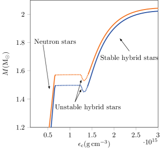
Figure 1: Constant angular momentum sequences depicting the gravitational mass $M$ as a function of the central energy density $\epsilon_{c}$ for EOS T9 of Bozzola et al. (2019) (labeled as EOS $\text{T9}_{0}$ in this work). We show the non-rotating sequence (lower blue line) and a sequence where $cJ/GM_{\odot}^{2}=1.0$ (upper orange line). Along each sequence we highlight the segments wherein twin stars roughly reside using dotted lines. We point out different segments of each sequence corresponding to stable neutron stars, stable hybrid stars, and unstable hybrid stars.

In this section we discuss the EOSs considered in this work. The EOSs were chosen such that they are representative of the diversity of EOSs treated in Paschalidis et al. (2018); Bozzola et al. (2019). Current constraints on the dense matter EOS allow for high-density quark deconfinement phase transitions. Hybrid EOSs vary widely and lead to a wide range of observable properties (see Baym et al. (2018) and references therein for a review of viable models of hadron-quark hybrid EOSs). A full exploration of the space of astrophysically consistent hybrid EOSs is beyond the scope of the present work, and our focus is on hybrid EOSs with phase transitions with a large jump in energy density, such that a third family of stable compact objects emerges.

Before we proceed further, in Fig. 1 we present a gravitational mass–central energy density plot, to show the branches of stable and unstable compact objects for the T9 EOS in Bozzola et al. (2019), which exhibits a first-order phase transition. The plot shows regions of the sequences corresponding to stable neutron stars, stable hybrid stars, and unstable hybrid stars for non-rotating stars (lower blue line), and a constant-angular momentum sequence with $cJ/GM_{\odot}^{2}=1.0$ (upper orange line). We also highlight segments of the sequences wherein twin stars roughly reside using dotted lines. According to the turning-point criterion for stability Friedman et al. (1988); Cook et al. (1992, 1994a, 1994b), along sequence of stars of constant entropy $S$, and constant angular momentum $J$, instability arises when

$$\dfrac{\partial M}{\partial\epsilon_{\rm c}}\Bigg{\rvert}_{J,S}\leq 0,$$ (1)

where $M$ is the gravitational or Arnowitt-Deser-Misner (ADM) mass and $\epsilon_{\rm c}$ is the central energy density. The unstable twin star branches are shown by the arrows in Fig. 1, where Eq. (1) is satisfied.

II.1 Base EOSs with first-order phase transitions

We focus on two representative EOSs from each of the two classes of hybrid EOSs studied in Paschalidis et al. (2018) and Bozzola et al. (2019). Namely, we consider EOSs based on A4 and T9, following the naming convention introduced in Bozzola et al. (2019); in Paschalidis et al. (2018) the A4 and T9 models are labeled as ACB4 and ACS-II $j{=}0.9$, respectively. Since we modify these original EOSs, in this work we label as $\text{A4}_{0}$ and $\text{T9}_{0}$ the original EOSs designated as A4 and T9 in Bozzola et al. (2019), respectively. Both EOSs correspond to zero-temperature matter in beta equilibrium. Each EOS incorporates hadronic (quark) degrees of freedom below (above) a threshold transition energy density density, $\epsilon_{\rm tr}$.

Among the different features between the EOSs are the parametrization of the pressure in the different phases. EOS $\text{A4}_{0}$ includes a parametrization of the pressure as a 4-segment piecewise polytrope,

$$P=\kappa_{i}\rho_{0}^{\Gamma_{i}},$$ (2)

where the index $i$ corresponds to the segment of the EOS and runs from 1 to 4 in the case of $\text{A4}_{0}$, $\rho_{0}$ is the rest-mass density, and $\kappa_{i}$ ($\Gamma_{i}$) is the polytropic constant (adiabatic exponent) corresponding to segment $i$. The specific values for $\kappa_{i}$ and $\Gamma_{i}$, as well as the values of number densities which demarcate each segment $n_{i}$, are listed in Tab. II of Paschalidis et al. (2018). EOS $\text{T9}_{0}$ includes a hadronic phase EOS calculated using density functional theory Colucci and Sedrakian (2013) and the quark phase EOS is calculated using the MIT bag model Witten (1984); Haensel et al. (1986); Alcock et al. (1986); Zdunik (2000). The pressure in the quark phase for EOS $\text{T9}_{0}$ is parametrized assuming a constant sound speed $c_{\rm s}$ as

$$P(\epsilon)=\begin{cases}P_{\text{tr}}&\epsilon_{\text{tr}}^{\text{T9}_{0}}\leq\epsilon\leq 1.9\epsilon_{\text{tr}}^{\text{T9}_{0}}\,,\\ P_{\text{tr}}+c_{\rm s}^{2}(\epsilon-1.9\epsilon_{\text{tr}}^{\text{T9}_{0}})&\epsilon\geq 1.9\epsilon_{\text{tr}}^{\text{T9}_{0}}\,,\end{cases}$$ (3)

where $c_{\rm s}=1.0$, $\epsilon$ is the energy density, $P_{\text{tr}}$ is the pressure of the hadronic phase at $\epsilon_{\text{tr}}^{\text{T9}_{0}}$, and the relativistic sound speed is defined as

$$c_{\rm s}^{2}\equiv\dfrac{\partial P}{\partial\epsilon}.$$ (4)

As shown in Paschalidis et al. (2018); Bozzola et al. (2019), a key difference between EOSs $\text{A4}_{0}$ and $\text{T9}_{0}$ is that the former is an example of an EOS that gives high-mass ($\sim 2M_{\odot}$) twin stars, while the latter results in low-mass ($\sim 1.5M_{\odot}$) twin stars. Another key difference between EOSs $\text{A4}_{0}$ and $\text{T9}_{0}$ is the response of their equilibrium configurations to rotation. For EOS $\text{A4}_{0}$, sequences of increasing angular momentum undergo a relatively large increase in mass for models with central energy density $\epsilon_{\text{tr}}^{\text{A4}_{0}}\lesssim\epsilon_{\rm c}\lesssim 1.78\epsilon_{\text{tr}}^{\text{A4}_{0}}$, which is roughly the region corresponding to the phase transition. This relative increase results in the maximum mass stable hybrid star having a smaller mass than the maximum mass hadronic star at large values of the angular momentum. On the contrary, for the $\text{T9}_{0}$ EOS there is a comparable increase in mass for models at all values of the energy density, which results in the maximum mass hybrid star having a larger mass than the maximum mass hadronic star at all values of the angular momentum. Considering these key differences between EOSs A4 and T9, we aim to qualitatively cover a considerable part of the space of hybrid hadron-quark EOSs.

II.2 The challenge of evolving EOSs with first-order phase transitions

The original $\text{A4}_{0}$ and $\text{T9}_{0}$ treat the phase transition region using a Maxwell construction. As a result, the EOSs have constant pressure during the phase transition which implies that the speed of sound vanishes ($c_{\rm s}=0$) for the corresponding values of the energy density. This is a problem for fluid dynamics and numerical evolutions, because when the sound speed vanishes the principal symbol of the equations of relativistic fluid dynamics does not possess a complete set of eigenvectors (as a straightforward check of the principal matrix in Font et al. (1994) can demonstrate). Hence the system of partial differential equations is only weakly hyperbolic Bertil and Heinz-Otto Kreiss (2013). For quasilinear partial differential equations weak hyperbolicity generally implies an ill-posed initial value problem Bertil and Heinz-Otto Kreiss (2013), which precludes stable numerical integration. Thus, EOSs with zero speed of sound can result in unstable numerical integration. To overcome this problem, we raise the value of the sound speed over the phase transition region. However, the modification is done such that the third family does not disappear as we explain in the following subsection.

II.3 Modified EOSs

One way to modify EOSs with first-order phase transitions so that the sound speed does not vanish is to change the type of construction method for matching the hadronic and the quark phases. This can be achieved by the well-known Glendenning construction Glendenning (1992), which leads to a smooth variation of the pressure over the phase transition region. However, the Glendenning and Maxwell constructions are two limits of the more general, and perhaps more physical, “pasta phase” construction Maslov et al. (2019). Other “smoothing” procedures were introduced in Abgaryan et al. (2018), demonstrating that the third family of compact stars does not depend on the existence of a first-order phase transition. Moreover, the modifications that were presented in the phase transition region are smooth enough to be represented with a piecewise polytrope. Additionally, piecewise polytropic parameterizations are able to capture the dynamics of the phenomena we are interested in, including the minimum-mass neutron star instability Colpi et al. (1993). This motivates the approach that we follow in the present work that we next turn to.

Given that piecewise polytropes simplify numerical hydrodynamic simulations, we first employ an 11-branch piecewise polytrope to fit both the $\text{A4}_{0}$ and $\text{T9}_{0}$ underlying EOSs, such that the pressure as a function of rest-mass density is described by Eq. (2). The first 4 branches of our fits are reserved for the crust, and for convenience we adopt the piecewise polytropic representation of the SLy Douchin and Haensel (2001) EOS, provided in Tab. II of Read et al. (2009). For a given EOS, we match our piecewise polytropic representation with the piecewise polytropic SLy parametrization at the lowest possible energy density at which the two EOSs intersect. We ensure that the pressure in our resulting EOSs is monotonically increasing with rest-mass density. We have also verified that the choice of crust EOS leaves the equilibrium stellar configurations used in our set of initial data practically the same as when using the baseline EOS tables.

Table 1: Properties of piecewise polytropic representations for the EOSs used in this work. We list the polytropic constants $\kappa_{i}$ (in cgs units determined by Eq. (2)), adiabatic exponents $\Gamma_{i}$, and segment-dividing rest-mass densities $\rho_{0,i}$ (in units of ${10}^{15}\text{\,}\mathrm{g}\text{\,}{\mathrm{cm}}^{-3}$) for each segment $i$. We list the sound speed at the start of the phase transition $c_{\rm s}^{\rm tr}$ (in units of the speed of light $c$) and the rest-mass densities corresponding to the start and end of the phase transition transition $\rho_{0,\rm tr}^{i}$ and $\rho_{0,\rm tr}^{f}$, respectively (in units of ${10}^{15}\text{\,}\mathrm{g}\text{\,}{\mathrm{cm}}^{-3}$). Note that the information for segments $1-4$ correspond to the SLy EOS Read et al. (2009). The polytropic information for EOS $\text{A4}_{0}$ can be found in Tab. II of Paschalidis et al. (2018) in the entry corresponding to EOS ACB4.

EOS	$i$	$k_{i}$	$\Gamma_{i}$	$\rho_{0,i}$	$c_{\rm s}^{\rm tr}$	$\rho_{0,\rm tr}^{i}$	$\rho_{0,\rm tr}^{f}$
$\text{A4}_{0}$	–	–	–	–	0.0	0.57	1.0
A4	1	$6.11\times 10^{+12}$	1.584	–	0.097	0.53	0.91
	2	$9.54\times 10^{+14}$	1.287	$2.44\times 10^{-8}$
	3	$4.79\times 10^{+22}$	0.062	$3.78\times 10^{-4}$
	4	$3.59\times 10^{+13}$	1.359	$2.63\times 10^{-3}$
	5	$6.50\times 10^{+15}$	1.186	0.02
	6	$6.62\times 10^{+03}$	2.060	0.05
	7	$5.40\times 10^{-04}$	2.559	0.16
	8	$3.59\times 10^{-38}$	4.921	0.29
	9	$1.15\times 10^{+32}$	0.200	0.53
	10	$1.65\times 10^{-25}$	4.000	0.91
	11	$2.09\times 10^{-10}$	3.000	1.27
$\text{T9}_{0}$	–	–	–	–	0.0	0.66	1.0
T9	1	$6.11\times 10^{+12}$	1.584	–	0.1	0.60	1.08
	2	$9.54\times 10^{+14}$	1.287	$2.44\times 10^{-8}$
	3	$4.79\times 10^{+22}$	0.062	$3.78\times 10^{-4}$
	4	$3.59\times 10^{+13}$	1.359	$2.63\times 10^{-3}$
	5	$3.75\times 10^{+06}$	1.870	0.04
	6	$1.43\times 10^{-03}$	2.536	0.14
	7	$1.02\times 10^{-15}$	3.377	0.29
	8	$3.03\times 10^{+30}$	0.3	0.60
	9	$2.52\times 10^{-49}$	5.56	1.08
	10	$1.16\times 10^{-18}$	3.535	1.38
	11	$9.91\times 10^{-02}$	2.427	1.88

Beyond the point at which we match with the SLy crust, we fit the underlying EOSs using the remaining 7 branches. Our fitting algorithm follows that of Read et al. (2009), which minimizes the relative error in the pressure between the underlying EOSs and their corresponding fits. There are two key sets of parameters which determine the optimal fit of an arbitrary tabulated EOS using piecewise polytropes. The first set of parameters is the rest-mass densities which demarcate the boundaries between neighboring polytropic segments $\rho_{0,i}$. The second set of parameters corresponds to the polytropic constants $\kappa_{i}$ and adiabatic exponents $\Gamma_{i}$ which provide a fit to the underlying EOS in question. In the following, we briefly discuss the algorithm used to determine these two sets of parameters. We begin by evenly dividing the range of rest-mass densities at which we fit the EOS beyond the crust into log-equispaced intervals. This division of rest-mass density serves as an initial guess for the optimal set of $\rho_{0,i}$. To avoid interpolation where possible, we ensure that the set of dividing rest-mass densities $\rho_{0,i}$ corresponds to points in the tabulated underlying EOS. The remainder of the algorithm is carried out to optimize the set of $\rho_{0,i}$, where we focus on the optimization of one polytropic segment at a time:

1. Given the set of dividing rest-mass densities $\rho_{0,i}$, we use the tabulated EOS to evaluate the corresponding set of dividing pressures $P_{i}$.

2. We determine the polytropic constants and adiabatic exponents for the polytropic fit using the following expressions:

   1. The adiabatic exponents are determined, assuming continuity between segments, as

      $$\Gamma_{i}=\dfrac{\log\left(P_{i}/P_{i-1}\right)}{\log\left(\rho_{0,i}/\rho_{0,i-1}\right)}$$ (5)

   2. The polytropic constants are then determined as

      $$\kappa_{i}=\dfrac{P_{i}}{\rho_{0,i}^{\Gamma_{i}}}.$$ (6)

   We highlight that the set of polytropic constants $\kappa_{i}$ are not independent of the adiabatic exponents $\Gamma_{i}$. Once we set the transition densities $\rho_{0,i}$, we then use these and the underlying EOS to determine the adiabatic exponents (step 2a. above), which in turn provide the polytropic constants (step 2b. above).

3. We evaluate the root-mean-square (RMS) error between a linear interpolation of the tabulated pressure and the polytropic fit to the pressure at values of the rest-mass density $\rho_{0}$ which span the entire range of rest-mass densities in the table. In particular, the RMS error is calculated as

   $$\text{RMS}[P]\equiv\sqrt{\sum_{n}^{N}\dfrac{\left(P_{\text{tab}}(\rho_{0,n})-P_{\text{poly}}(\rho_{0,n})\right)^{2}}{N}},$$ (7)

   where $\rho_{0,n}$ corresponds to the elements of a list of $N$ rest-mass densities. We typically choose $N=1000$ and choose the rest-mass densities $\rho_{0,n}$ such that they are log-equispaced between the minimum and maximum values of the rest-mass density in the table. $P_{\text{tab}}$ is the pressure corresponding to the tabulated underlying EOS linearly interpolated to the rest-mass density $\rho_{0,n}$, and $P_{\text{poly}}$ is the pressure corresponding to the piecewise polytropic fit at $\rho_{0,n}$. We employ linear interpolation because the underlying table is dense and to avoid oscillations arising from discontinuous pressure derivatives around sharp features of the EOS such as the start and end of the phase transition. Eq. (7) allows us to determine the RMS error over the entire EOS for a particular choice of $\rho_{0,i}$ corresponding to the current EOS segment.

4. We then vary $\rho_{0,i}$ for the current EOS segment until the RMS error is minimized. Once this is done, we focus on the neighboring segment and repeat the algorithm starting at step 1 above, until all segments have been chosen such that the RMS error is minimized for each segment separately. Once we have updated the values of all $\rho_{0,i}$ that constitutes one iteration in the fitting algorithm.

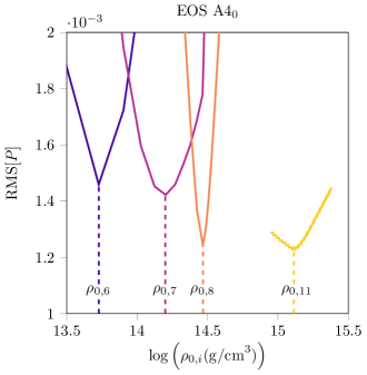
Figure 2: Example of the root-mean-square error in the pressure as a function of the choice for the dividing rest-mass density corresponding to segments 6, 7, 8, and 11 (dark blue, magenta, orange, and yellow lines, respectively) of the polytropic fit for EOS $\text{A4}_{0}$. For each segment, we mark the value of $\rho_{0,i}$ that results in the minimum RMS error (and are thus optimal choices) with a dashed vertical line of the same color.

We perform multiple iterations of the fitting algorithm until the minimum RMS error saturates and no longer decreases, thereby ensuring that the set of $\rho_{0,i}$ is optimal. In Fig. 2 we show, as an example, the RMS error corresponding to the first iteration of the fitting algorithm in the case of the $\text{A4}_{0}$ EOS. For each polytropic segment, depicted by different color lines in Fig. 2, the RMS error clearly reaches a minimum at the best choice of $\rho_{0,i}$ for that segment. We note that, as suggested by the curves in Fig. 2, we only optimize the dividing rest-mass densities corresponding to segments 6, 7, 8, and 11 because segments 1-4 correspond to the SLy crust, segment 5 corresponds to the point at which the crust matches the high density EOS, and segments 9 and 10 correspond to the start and end of the phase transition, respectively. As such, $\rho_{0,6},\rho_{0,7},\rho_{0,8}$, and $\rho_{0,11}$ are the only members of $\rho_{0,i}$ which should be optimized, and all others are left fixed.

In fitting each EOS with piecewise polytropes, we have full control of the adiabatic index (and thus the sound speed) during the phase transition $\Gamma_{\text{tr}}$. Note that fixing neighboring members of $\rho_{0,i}$ at the points corresponding to the start and end of the phase transition ensures that we fit that region with a single polytrope. We experimented with several values of $\Gamma_{\text{tr}}$, and chose values slightly above the lowest one for which the evolution of stable equilibrium hybrids stars did not exhibit numerical instabilities. We discuss the evolution of such models in App. A. The value chosen for $\Gamma_{\text{tr}}$ corresponds to $c_{\rm s}^{\text{tr}}=0.097$ ($c_{\rm s}^{\text{tr}}=0.1$) at rest-mass density $\rho_{0}=$5.3\text{\times}{10}^{14}\text{\,}\mathrm{g}\text{\,}{\mathrm{cm}}^{-3}$$ ($\rho_{0}=$6.0\text{\times}{10}^{14}\text{\,}\mathrm{g}\text{\,}{\mathrm{cm}}^{-3}$$) for EOS A4 (T9). In Tab. 1 we list the polytropic constants $\kappa_{i}$, adiabatic exponents $\Gamma_{i}$, and dividing rest-mass densities $\rho_{0,i}$ that provide the fit to our nonzero sound speed versions of the $\text{A4}_{0}$ and $\text{T9}_{0}$ EOSs. Henceforth, we use the labels A4 and T9 to correspond to the piecewise polytropic, nonzero sound speed EOSs used in this work and summarized in Tab. 1. Note that in Tab. 1, the polytropic information is listed such that for $\rho_{0}>\rho_{0,i}$, the pressure is given by $P=\kappa_{i}\rho_{0}^{\Gamma_{i}}$. Hence, the first entry for $\rho_{0,i}$ is left blank because the first segment of the EOS may begin at any rest-mass density below $\rho_{0,2}$.

III Initial Data

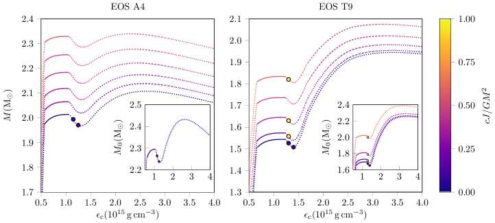
Figure 3: Left panel: Sequences of constant angular momentum, and zero entropy depicting the gravitational mass $M$ as a function of the central energy density $\epsilon_{c}$ for EOS A4. The colorbar corresponds to the dimensionless spin $a=cJ/GM^{2}$ along each sequence. For each sequence we highlight the additional stable models introduced by modifying the polytropic fit to the underlying $\text{A4}_{0}$ EOS using solid line segments. We mark the models that comprise our set of initial data using circles (dark blue for non-rotating and bright yellow for rotating). In the inset we show the rest mass $M_{0}$ as a function of central energy density $\epsilon_{\rm c}$ for sequences which correspond to our initial data for this EOS. Right panel: Same as left panel but for EOS T9.

In this section we discuss the methods for generating our initial data and the properties of the initial configurations we considered.

III.1 Methods

We construct initial data with the code of Cook et al. (1992, 1994a, 1994b), which solves Einstein’s equations coupled to the equations of hydrostationary equilibrium for a perfect fluid assuming stationarity and axisymmetry. The code adopts the following spacetime metric Cook et al. (1994a) (see Paschalidis and Stergioulas (2017) for a review of other line elements used in the literature)

$$ds^{2}=-e^{\gamma+\rho}dt^{2}+e^{2\alpha}(dr^{2}+r^{2}d\theta^{2})+e^{\gamma-\rho}r^{2}\sin^{2}\theta(d\phi-\omega dt)^{2},$$ (8)

where $r$, $t$, $\theta$, and $\phi$ correspond to the usual spherical coordinates, and $\gamma$, $\rho$, $\omega$, and $\alpha$ are metric potentials which are functions of $r$ and $\theta$ only. The perfect fluid stress-energy tensor is given by

$$T^{ab}=\rho_{0}hu^{a}u^{b}+Pg^{ab},$$ (9)

where $u^{a}$ is the fluid four velocity and $h$ is the specific enthalpy, given by

$$h=1+\varepsilon+\dfrac{P}{\rho_{0}},$$ (10)

where $\varepsilon$ is the specific internal energy . To close the system of equations, the EOSs described in Sec. II are supplied.

III.2 Equilibrium configurations

Using our EOSs A4 and T9 we build equilibrium configurations of compact stars. In Fig. 3, we show constant angular momentum sequences for the A4 EOS (left panel) and T9 EOS (right panel) for rigidly rotating stars. As demonstrated in the figure, our modified EOSs give rise to a third family of compact stars, including branches of stable and unstable twin stars. In addition, the inclusion of rotation results in a relative increase in mass for different regions of the EOS fits, as previously described for the underlying EOSs. More specifically, we find that the A4 EOS is most alike the $\text{A4}_{0}$ EOS beyond the phase transition region, and results in a close match of the maximum mass hybrid star with $\sim 0.2\%$ relative difference in the mass, while it results in a $\sim 2\%$ difference in the maximum mass star on the hadronic branch. On the other hand, the T9 EOS most closely matches the $\text{T9}_{0}$ EOS below the phase-transition region, resulting in a close match of the maximum mass hadronic star with less than $0.1\%$ relative difference in the mass, while it results in a $\sim 4\%$ relative difference in the maximum mass of the third-family branch. Thus, our fits provide good approximations to the underlying EOSs without the shortcoming of a zero sound speed over the phase transition region.

The key difference introduced into the EOSs by increasing the sound speed is a change from a sharp, first-order phase transition to a smoother transition between phases. As mentioned earlier, both sharp and smooth phase transitions are consistent with a high-density quark deconfinement phase transition, and each scenario has been considered in the study of hybrid stars in the past Hempel et al. (2009); Yasutake and Kashiwa (2009); Bhattacharyya et al. (2010); Yasutake et al. (2011). In the context of the turning-point instability, increasing the sound speed over the phase transition region leads to a nonzero first derivative $M^{\prime}(\epsilon_{c})$ over the span of the transition, where before it was 0, and hence the $\text{A4}_{0}$ and $\text{T9}_{0}$ EOSs contained only turning-point marginally unstable models. Compared to the original $\rm A4_{0}$ and $\rm T9_{0}$, our A4 and T9 EOSs have an extended second family of compact objects that in addition to neutron stars now also includes stars whose maximum density is above the phase transition threshold, and hence are hybrid stars. Moreover, the maximum mass configuration in the second family is also a hybrid star. This is a result of the mixed hadron-quark phase introduced by modifying of the original EOSs.

Table 2: Properties of the initial unstable equilibrium twin star configurations considered in this work. For each model we show the central energy density $\epsilon_{c}$ and rest-mass density $\rho_{0,\rm c}$ in units of ${10}^{15}\text{\,}\mathrm{g}\text{\,}{\mathrm{cm}}^{-3}$, the ADM mass $M$ and rest mass $M_{0}$ in units of $\text{\,}\mathrm{M}_{\odot}$, the compactness $C\equiv GM/R_{c}c^{2}$ (where $R_{c}$ is the equatorial circumferential radius), the ratio of polar to equatorial radii $r_{p}/r_{e}$, and dimensionless spin $a\equiv cJ/GM^{2}$. For each model, in the last two columns we also list the central rest-mass density (in units of ${10}^{15}\text{\,}\mathrm{g}\text{\,}{\mathrm{cm}}^{-3}$) of the lower (second family) and higher density (third family) stable stars with rest mass equal to the unstable configuration. The last line in the table corresponds to the minimum mass unstable hybrid twin star with the T9 EOS, which does not have a corresponding higher-density configuration on the stable third-family branch.

EOS	$\epsilon_{c}$	$\rho_{0,\rm c}$	$M$	$M_{0}$	$C$	$\frac{r_{p}}{r_{e}}$	$a$	$\rho_{0,c,\rm low}$	$\rho_{0,c\rm high}$
A4	1.15	0.97	1.99	2.27	0.21	1.00	0.00	0.61	1.21
	1.25	1.04	1.97	2.24	0.22	1.00	0.00	0.53	1.13
T9	1.30	1.12	1.53	1.68	0.17	1.00	0.00	0.73	1.25
T9	1.30	1.12	1.56	1.71	0.17	0.96	0.20	0.70	1.25
	1.30	1.12	1.63	1.80	0.17	0.87	0.40	0.76	1.28
	1.30	1.12	1.82	2.00	0.17	0.68	0.60	0.68	1.27
T9	1.40	1.19	1.50	1.65	0.17	1.00	0.00	0.62	–

In Fig. 3 we mark with filled circles the points along the constant angular momentum sequences which correspond to our set of initial data. This set samples a range of masses of twin stars on the unstable branch, with the lowest and highest mass stars having $M\approx 1.5M_{\odot}$, and $M\approx 2.0M_{\odot}$, respectively. Some of our models have rest masses which are greater than that of the corresponding maximum mass hadronic stars $M_{\rm max}^{\rm had}$, leading to the possibility that they settle into the stable hybrid configurations in the second family introduced after smoothing the phase transition transition (see insets in each panel of Fig. 3 for constant $J$ sequences which show the rest mass $M_{0}$ as a function of the energy density). In Fig. 3 we highlight these additional stable models using solid line segments along each constant angular momentum sequence. We discuss the possibility of settling into these additional stable configurations in Sec. V. Our rotating models (marked by yellow filled circles in the right panel of Fig. 3) are chosen by considering constant angular momentum sequences which contain stable stars on both the hybrid and hadronic branches and locating models which satisfy Eq. (1). We include relevant properties for the set of initial data in Tab. 2.

III.3 Initial perturbations

Table 3: Main set of cases considered in this work. For each model we list the model name (see text body for model naming convention), the EOS, the central energy density in units of ${10}^{15}\text{\,}\mathrm{g}\text{\,}{\mathrm{cm}}^{-3}$, the dimensionless spin $a=cJ/GM^{2}$, and the value of the perturbation parameter $\xi$ in Eq. (11). The final entry, model $\rm MMT9_{1.4}^{-2\%}$, corresponds to the evolution of the minimum-mass non-rotating hybrid star for the T9 EOS in the case where $2\%$ of the rest mass is removed at the start of the simulation.

Model	EOS	$\epsilon_{c}$	$a$	$\xi$
$\rm A4_{1.15}^{-0.01}$	A4	1.15	0.0	-0.01
$\rm A4_{1.15}^{0}$	A4	1.15	0.0	0.0
$\rm A4_{1.15}^{+0.01}$	A4	1.15	0.0	0.01
$\rm A4_{1.25}^{-0.01}$	A4	1.25	0.0	-0.01
$\rm A4_{1.25}^{0}$	A4	1.25	0.0	0.0
$\rm A4_{1.25}^{+0.01}$	A4	1.25	0.0	0.01
$\rm T9_{1.3}^{-0.01}$	T9	1.3	0.0	-0.01
$\rm T9_{1.3}^{0}$	T9	1.3	0.0	0.0
$\rm T9_{1.3}^{+0.01}$	T9	1.3	0.0	0.01
$\rm T9_{1.3}^{0.0}a_{0.2}$	T9	1.3	0.2	0.0
$\rm T9_{1.3}^{-0.01}a_{0.2}$	T9	1.3	0.2	-0.01
$\rm T9_{1.3}^{0.0}a_{0.4}$	T9	1.3	0.4	0.0
$\rm T9_{1.3}^{-0.01}a_{0.4}$	T9	1.3	0.4	-0.01
$\rm T9_{1.3}^{0.0}a_{0.6}$	T9	1.3	0.6	0.0
$\rm T9_{1.3}^{-0.01}a_{0.6}$	T9	1.3	0.6	-0.01
$\rm MMT9_{1.4}^{-2\%}$	T9	1.4	0.0	0.0

For each configuration presented in Tab. 2 we consider the effects of seeding a small perturbation at the start of the simulation. We focus on quasi-radial perturbations which are seeded by perturbing the pressure at $t=0$ everywhere in the star. The form of the pressure perturbation is

$$P(t=0,\mathbf{x})\longrightarrow(1+\xi)P(t=0,\mathbf{x}),$$ (11)

where $\mathbf{x}$ indicates the spatial coordinates, and $\xi$ can be either positive or negative in cases where we add or deplete pressure, respectively. Our main set of simulations is summarized in Tab. 3, and consists of 16 cases. The naming convention for the models presented in Tab. 3 is as follows. The model name begins with the EOS label, followed by a superscript corresponding to the value of the perturbation parameter in Eq. (11) and a subscript corresponding to the value of the initial central energy density (in units of ${10}^{15}\text{\,}\mathrm{g}\text{\,}{\mathrm{cm}}^{-3}$) which determines the model’s location on the unstable branch. For rotating configurations, the model name is followed by the letter ‘a’ (corresponding to the dimensionless spin)

$$a\equiv\dfrac{cJ}{GM^{2}},$$ (12)

and a subscript corresponding to the value of $a$. For example, the non-rotating model corresponding to the A4 EOS with $\epsilon_{\rm c}=$1.15\text{\times}{10}^{15}\text{\,}\mathrm{g}\text{\,}{\mathrm{cm}}^{-3}$$ under a $1\%$ positive pressure perturbation is labeled $\rm A4^{+0.01}_{1.15}$, while the rotating model corresponding to the T9 EOS with $\epsilon_{\rm c}=$1.3\text{\times}{10}^{15}\text{\,}\mathrm{g}\text{\,}{\mathrm{cm}}^{-3}$$ under a $1\%$ negative pressure perturbation and spin $a=0.4$ is labeled $\rm T9^{-0.01}_{1.3}a_{0.4}$. In Tab. 3 we also list the simulation $\rm MMT9_{1.4}^{-2\%}$, which corresponds to the evolution of the minimum mass non-rotating hybrid star for the T9 EOS, where $2\%$ of the initial rest mass is stripped at the start of the simulation (here we use $2\%$ and non 0.02 in the case label to indicate that it is not a pressure perturbation). Along with the simulations presented in Tab. 3 we also consider two simulations at varying grid resolutions corresponding to model $\rm A4^{-0.01}_{1.25}$, a set of simulations corresponding to stable hybrid stars used to asses the validity of each EOS, two simulations corresponding to different size initial perturbations for model $\rm T9_{1.3}^{-0.01}$, three simulations corresponding to stable branch hybrid twin stars used to consider the possibility of migration from the stable branch to the unstable regime, and several simulations corresponding to the lower and higher density equilibria with the same rest mass as that of particular models in Tab. 3 as comparison points. Our stable twin star and resolution studies are presented in App. A. Our study of dynamical migration from the stable hybrid branch is presented in App. B.

IV Evolution methods

In this section we describe the basic methods used in evolving the initial data outlined in Sec. III. We describe the evolution code, the grid hierarchy, and detail the different diagnostics used.

IV.1 Evolution code

To evolve the hydrodynamics and spacetime we use the code of Duez et al. (2005); Etienne et al. (2010a, 2015), which operates within the Cactus framework Allen et al. (2001) and employs Carpet Schnetter et al. (2004, 2006) for mesh refinement. The code solves the Einstein equations using the Baumgarte-Shapiro-Shibata-Nakamura formulation Shibata and Nakamura (1995); Baumgarte and Shapiro (1999) within the 3+1 formalism. Our gauge choice consists of “1+log” slicing for the lapse Bona et al. (1995) and the “Gamma-freezing” condition for the shift in first-order form Alcubierre et al. (2001, 2003); Etienne et al. (2008). The temporal evolution uses a fourth-order Runge-Kutta scheme with a Courant-Friedrichs-Lewy factor of 0.5. The fluid variables are evolved in flux-conservative form adopting high-resolution shock-capturing methods Etienne et al. (2010b, 2012). Our code is compatible with piecewise polytropic representations of realistic, cold, beta-equilibrated EOSs. We validate our approach to modify hybrid hadron-quark equations of state by evolving stable branch hybrid star models. We present the results of these evolutions in App. A. The code has been thoroughly tested in the past and demonstrated to be convergent. Of relevance to this work are the convergence tests in Paschalidis et al. (2011a).

IV.2 Grid hierarchy

For all evolutions in this work, we construct evolution grids, using fixed mesh refinement Schnetter et al. (2004, 2006), consisting of 7 nested boxes. The half-side length of the finest level is set to $1.5R_{c}$ (where $R_{c}$ is the initial hybrid star equatorial circumferential radius), and all subsequent levels have half-side length equal to twice that of the adjacent finer level. The canonical resolution used in our study is set such that the finest level contains at least 64 grid-points per $R_{c}$, so that the finest canonical grid spacing is given by $\Delta x_{1}=R_{c}/64$. All other levels have grid spacings $\Delta x_{n}=2\Delta x_{n-1}$, where $n\in(2,7)$ is the level number with larger $n$ meaning coarser level. In addition, we consider higher resolution simulations to assess convergence and invariance of our results with resolution. For higher resolution runs, we employ grids which are $1.25$ and $1.5$ times finer than the canonical-resolution grid, which we label the medium- and high-resolution cases, respectively. Note that there are at least 80 and 96 grid-points per $R_{c}$ for the medium- and high-resolution simulations, respectively. To reduce computational cost we employ reflection symmetry across the equatorial plane. To avoid singularities when converting the initial stellar solutions from spherical polar to the Cartesian coordinates used in the evolution, we shift the grid points in the y-direction by $\Delta y=0.001$ (in units where $(G/c^{2})${10}^{15}\text{\,}\mathrm{g}\text{\,}{\mathrm{cm}}^{-3}$$ equals 1), so that the origin is avoided. Such coordinate shifts have been shown to have a negligible effect on the dynamics of relativistic stars Espino and Paschalidis (2019).

IV.3 Diagnostics

We monitor several diagnostics to assess different aspects of the evolution including the evolution of the rest-mass density, the $L_{2}$ norm of the Hamiltonian and momentum constraints Etienne et al. (2008), and global conservation laws such as total rest-mass, total ADM mass, and angular momentum conservation. We also track the boundary between the hadronic and quark phases, which we define as the locus of points where the rest-mass density $\rho_{0}$ equals the value corresponding to the onset of the phase transition for a given EOS.

Although our initial configurations are in equilibrium, rotating models undergoing quasi-radial oscillations generate GWs. To investigate this, we extract GWs using the Newman-Penrose formalism Newman and Penrose (1962); Penrose (1963), in particular focusing on $s=-2$ spin-weighted spherical harmonic decompositions of the Newman-Penrose scalar $\Psi_{4}$. The coefficients of the spin-weighted decomposition are labeled $\Psi_{4}^{l,m}$, where $l$ and $m$ are the usual degree and order for the spherical harmonics. In all cases we focus on the dominant quasi-radial $l=2$, $m=0$ mode. We extract $\Psi_{4}^{l,m}$ from the numerical solution at fixed concentric spheres with increasing coordinate radii $r_{\rm ex}=\eta M$, where $\eta\in\left\{40,50,60,80,90,100\right\}$. For a suitable comparison to the GWs of similar systems Dimmelmeier et al. (2009); Haensel et al. (2016), we compute the gravitational wave strain $h$ from

$$\Psi_{4}=\ddot{h}_{+}-i\ddot{h}_{\times}.$$ (13)

adopting the fixed-frequency integration (FFI) Reisswig et al. (2011). The visualizations and GW analysis presented in this work were carried out using the kuibit Python package Bozzola (2021).

V Results

In this section we detail the results of the simulations listed in Tab. 3. We first discuss our non-rotating models, categorizing by the perturbation seeded at the beginning of the simulations. We highlight the key features in the evolution and point out the differences between the results for each EOS. We then present the results for rotating models and highlight the key differences in the dynamics introduced by rotation. Finally, we summarize the results of our study of the hybrid star minimum-mass instability.

V.1 Non-rotating models

Our set of non-rotating models consists of the first 9 entries in Tab. 3. The initial data for this set consists of three models: two correspond to the A4 EOS, and one to the T9 EOS. The initial data set also covers a range of central energy densities and masses in the unstable twin star branch. In general, we find that all non-rotating models in our study migrate toward the stable hadronic configuration, i.e., the neutron star with the same rest mass but lower maximum rest-mass density than the original configuration. Generally, adding (removing) pressure initially, such that $\xi>0$ ($\xi<0$), results in the configuration settling near the hadronic branch on a shorter (longer) timescale than cases wherein no perturbation was applied. Depending on the EOS and central energy density of the initial configuration, slight qualitative differences arise between the evolutions. However, all non-rotating models tend toward the hadronic branch (the second family of stable compact objects), showing that the outcome of the instability is independent of the perturbations we studied. In the following we consider the effect of each perturbation separately.

V.1.1 Equilibrium evolution

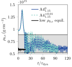
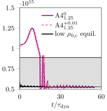
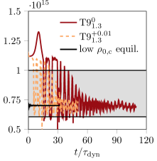
Figure 4: Left panel: Central rest-mass density $\rho_{0,\rm c}$ as a function of time (scaled by the dynamical time $\tau_{\rm dyn}$) for model $\rm A4_{1.15}^{0}$ under equilibrium evolution (solid lines) and model $\rm A4_{1.15}^{+0.01}$ with a positive pressure perturbation (dashed lines). Also shown is $\rho_{0,\rm c}$ for the lower-density equilibrium model with the same rest mass as that of the initial configuration (solid black line). We use horizontal black lines to mark the start (lower lines) and end (upper lines) of the phase transition and a gray band to mark the densities corresponding to the phase transition region. Center panel: Same as the left panel but for models $\rm A4_{1.25}^{0}$ and $\rm A4_{1.25}^{+0.01}$. Right panel: Same as the left and center panels but for models $\rm T9_{1.3}^{0}$ and $\rm T9_{1.3}^{+0.01}$.

In Fig. 4 we present the central rest-mass density as a function of time for the case of equilibrium evolution for all non-rotating models in our study. Note that in Fig. 4 the time is scaled by the dynamical time, given by $\tau_{\rm dyn}=1/\sqrt{\rho_{0,\rm max}(t=0)}$. The central rest-mass densities for models $\rm A4_{1.15}^{0}$, $\rm A4_{1.25}^{0}$, and $\rm T9_{1.3}^{0}$ are depicted in the left, center, and right panels of Fig. 4, respectively, using solid lines. We mark the densities corresponding to the phase transition region of the EOS using gray shaded regions in Fig. 4, such that central rest-mass densities below the gray shaded regions correspond to pure hadronic stars.

In the case of equilibrium evolution all non-rotating models in our study undergo an initial increase in the rest-mass density corresponding to contraction, which takes place early in the evolution. At this point the size of the quark core saturates, the EOS stiffens, and the models subsequently begin expanding. As the models expand the value of the central rest-mass density eventually becomes smaller than the threshold corresponding to the end of the phase transition $\rho_{0,\rm tr}^{f}$ and quickly drops to a value $\rho_{0,\rm c}\lesssim\rho_{0,\rm tr}^{i}$ (see Tab. 1 for the values of $\rho_{0,\rm tr}^{i}$ and $\rho_{0,\rm tr}^{f}$ for each EOS). The expansion reverts into a momentary collapse as the models begin to contract until $\rho_{0,\rm c}>\rho_{0,\rm tr}^{i}$, at which point the central rest-mass density jumps to a point above the end of the phase transition $\rho_{0,\rm c}\gtrsim\rho_{0,\rm tr}^{f}$. The models undergo several such bounces corresponding to radial oscillations while the core oscillates between the hadronic and quark phases. Eventually, the radial oscillations decay as the models settle into approximately steady states at lower central rest-mass densities.

The size and number of oscillations observed early in the evolution likely depends on the position of each model along the unstable branch (i.e., on the model’s central energy density and rest mass). Of the models considered, $\rm A4_{1.25}^{0}$ is the only one with rest mass lower than the maximum rest mass purely hadronic star – the configuration with central rest-mass density just below the phase transition threshold. In other words, models $\rm A4_{1.15}^{0}$ and $\rm T9_{1.3}^{0}$ have counterpart lower-density, stable equilibrium hybrid star models with the same rest mass, which are in the second family of compact objects (see solid segments of Fig. 3). We find significant oscillations throughout the evolutions of models $\rm A4_{1.15}^{0}$ and $\rm T9_{1.3}^{0}$ which peak inside the gray bands corresponding to the phase transition region in Fig. 4. However, we find a lack of such long-term oscillations in model $\rm A4_{1.25}^{0}$, possibly because this unstable twin star has a lower-density stable counterpart with max density below that of the phase transition threshold. Such a disparity in dynamics between unstable branch stars (whether or not their central regions oscillate within the phase transition region) may be tied to our EOSs where the quark deconfinement phase transition is not a first-order transition. For sharp, first-order phase transitions, all EOS models we are aware of produce unstable branch twin stars with corresponding lower-density neutron stars which have central rest-mass density lower than $\rho_{0,\rm tr}^{i}$. If the quark deconfinement phase transition is of first-order, the migration of unstable branch hybrid stars toward the hadronic branch may closely follow the evolution of model $\rm A4_{1.25}^{0}$. However, since the pasta phase reconstruction may be more natural, there may be a diversity in how unstable twin stars migrate toward the hadronic branch. The $\rm A4_{1.15}^{0}$ and $\rm T9_{1.3}^{0}$ models both undergo small but non-negligible late-time oscillations in the rest-mass density of approximately $\sim 5\%$ in amplitude. We evolved these models for more dynamical times than the $\rm A4_{1.25}^{0}$ model, which reveals that the amplitude of the rest-mass density oscillations continues to decrease, albeit at a slower rate compared to the initial oscillations.

For suitable comparisons we also consider the evolution of the stable lower-density equilibrium model with the same rest mass as that of the initial configuration of each model. We depict the central rest-mass density for these models with solid black lines in Fig. 4. In all cases the evolution of the lower-density counterparts show small ($\lesssim 1\%$) oscillations in the rest-mass density. It is worth noting that the final central rest-mass density of the lower-density counterparts agrees to within $\sim 0.08\%$, $\sim 1.5\%$, and $\sim 0.1\%$ with the final central rest-mass density of models $\rm A4_{1.15}^{0}$, $\rm A4_{1.25}^{0}$ and $\rm T9_{1.3}^{0}$, respectively. By the end of the evolutions it is clear that all unstable models are very close to their lower-density stable counterpart in the second family.

V.1.2 Positive initial pressure perturbation

The evolution of $\rho_{0,\rm c}$ for the case of positive pressure perturbations is shown by the dashed lines in Fig. 4. We generally find that adding a positive initial pressure perturbation results in evolutions that are similar to those without initial perturbation. Depending on the EOS, the key features of evolution may arise on a slightly shorter timescale. For instance, where model $\rm T9_{1.3}^{0.0}$ settled into a lower-density configuration with $\sim 5\%$ oscillations in the rest-mass density after $t\approx 60\tau_{\rm dyn}$, we find that adding pressure drives the initial configuration to a similar state by $t\approx 30\tau_{\rm dyn}$. The timescale on which models $\rm A4_{1.15}^{+0.01}$ and $\rm A4_{1.25}^{+0.01}$ settle to lower densities is almost identical to models $\rm A4_{1.15}^{0}$ and $\rm A4_{1.25}^{0}$, respectively.

Depending on the EOS, the early evolution in cases with positive pressure perturbations show small differences to the cases of equilibrium evolution. For models $\rm A4_{1.15}^{+0.01}$ and $\rm A4_{1.25}^{+0.01}$ we observe an initial small expansion, which is followed by contraction and subsequent evolution similar to the cases wherein no perturbations were excited. However, model $\rm T9_{1.3}^{+0.01}$ undergoes an initial expansion, without contraction, which coincides with an initial decrease in the central rest-mass density. The model continues expanding until the quark phase disappears from the stellar center. The model then undergoes a number of bounces and the evolution proceeds in a qualitatively similar fashion to that of model $\rm T9_{1.3}^{0}$.

The differences in the early stages of evolution between model $\rm T9_{1.3}^{+0.01}$ and those corresponding to the A4 EOS may be attributed to the EOS stiffness in the quark phase immediately above the phase transition region. The first polytropic segment after the phase transition region (listed in Tab. 1 as segment 10 and 9 for EOSs A4 and T9, respectively) corresponds to the part of the EOS that is sampled in the central region of these stars. As such, the central regions of the initial configurations are significantly stiffer for models built using the T9 EOS than for those built with the A4 EOS.

V.1.3 Pressure depletion

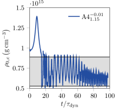
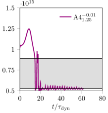
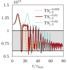
Figure 5: Left panel: Central rest-mass density $\rho_{0,\rm c}$ as a function of time (scaled by the dynamical time $\tau_{\rm dyn}$) for model $\rm A4_{1.15}^{-0.01}$ under a negative pressure perturbation. We use horizontal black lines to mark the start (lower lines) and end (upper lines) of the phase transition and a gray band to mark the densities corresponding to the phase transition region. Center panel: Same as the left panel but for model $\rm A4_{1.25}^{-0.01}$. Right panel: Same as the left and center panels but for model $\rm T9_{1.3}^{-0.01}$. Also shown are $\rho_{0,\rm c}$ for model $\rm T9_{1.3}^{-0.005}$ with $0.5\%$ pressure depletion (light orange dashed line) and $\rm T9_{1.3}^{-0.02}$ with $2\%$ pressure depletion (blue dotted line).

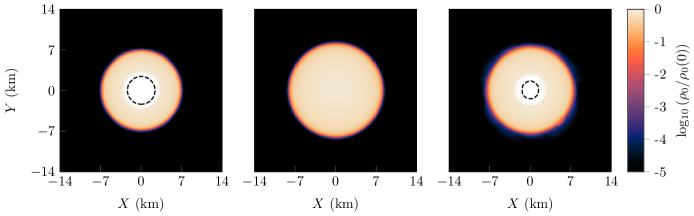
Figure 6: Left panel: Equatorial snapshot of the rest-mass density for model $\rm A4_{1.15}^{-0.01}$ at time $t\approx 10\tau_{\rm dyn}$, which corresponds to the peak of the central rest-mass density. We outline the region with rest-mass density larger than the end of the phase transition (corresponding to the quark core, shown in white) with a black dashed line. At this stage the model exhibits a large quark core. Center panel: Same as the left panel, but for time $t\approx 15\tau_{\rm dyn}$, which corresponds to the disappearance of the quark phase and the expansion of the model following the initial contraction. Right panel: Same as the left and center panels, but for time $t\approx 40\tau_{\rm dyn}$, which corresponds to a relative peak in the rest-mass density and the re-appearance of the quark core.

In this section we describe our results for an initial perturbation that depletes ($\xi<0$) a small fraction of the pressure everywhere. This is designed to test if the unstable configuration can be pushed to the stable twin star counterpart. In Fig. 5 we show the central rest-mass density in the case of pressure depletion. We generally find that relative to the equilibrium evolution, pressure depletion tends to delay the timescale on which some key features arise. Similarly to the cases of equilibrium evolution and positive pressure perturbations, the models considered under pressure depletion settle at lower central rest-mass densities toward the second family branch. For all models under pressure depletion we observe an initial increase in rest-mass density. This initial increase in rest-mass density leads to the growth of the quark core, such that a larger part of the core is above the densities of the phase transition region, where the EOS stiffens again. The stiffening of the EOS at these high densities leads to a bounce, and the configurations enter an expansion phase, which results in a decrease of the central rest-mass density. Once the central rest-mass density falls below the critical value corresponding to the end of the phase transition (upper solid black line in the left panel of Fig. 5), it quickly drops to the rest-mass density corresponding to the start of the phase of transition (lower solid black line) and the quark core disappears. As the core enters a softer part of the EOS, the pressure support becomes weaker, and the star quickly reverts into a momentary collapse. The cycle repeats and the maximum rest-mass density exhibits strong oscillations as the central region bounces between the quark and hadronic phases. Similar to cases wherein no explicit perturbation was excited, such oscillations eventually decay and the models settle to lower central rest-mass densities. Depending on the properties of the initial configurations (such as central energy density and mass), pressure depletion may induce a larger number of such oscillations compared to cases with no explicit perturbation.

The $\rm A4_{1.15}^{-0.01}$ model (left panel of Fig. 5) undergoes strong bounces between the quark and hadronic phases for the first $t\approx 60\tau_{\rm dyn}$ of evolution, while the oscillations in the central rest-mass density are damped as the model settles to the lower-density stable equilibrium model with the same rest mass as that of the initial configuration (note that for models $\rm A4_{1.15}^{0.0}$ and $\rm A4_{1.15}^{+0.01}$ the strong oscillations were damped after $t\approx 20\tau_{\rm dyn}$). Model $\rm T9_{1.3}^{-0.01}$ (right panel of Fig. 5) similarly exhibits strong oscillations for longer ($t\approx 40\tau_{\rm dyn}$) than models $\rm T9_{1.3}^{0.0}$ ($t\approx 30\tau_{\rm dyn}$) and $\rm T9_{1.3}^{+0.01}$ ($t\approx 20\tau_{\rm dyn}$). In the case of the $\rm A4_{1.25}^{-0.01}$ model (center panel of Fig. 5) we find that the configuration settles at the lower-density equilibrium model with the same rest mass as that of the initial configuration on a comparable (but slightly longer) timescale than the corresponding equilibrium evolution case. Model $\rm A4_{1.25}^{-0.01}$ shows oscillations of a comparable number, duration, and amplitude to model $\rm A4_{1.25}^{0.0}$, suggesting that this initial configuration has the highest propensity to migrate toward the stable second-family branch as discussed in Sec. V.1.1.

In Fig. 6 we show snapshots of equatorial contours of the rest-mass density at key points corresponding to the evolution of model $\rm A4_{1.15}^{-0.01}$. We outline the quark phase (shown in white), with $\rho_{0}>\rho_{0,\rm tr}^{f}$, using black dashed lines. The left panel of Fig. 6 depicts the saturation of the quark core size during the initial contraction stage of the model at $t\approx 10\tau_{\rm dyn}$. The center panel of Fig. 6 corresponds to the disappearance of the quark core during the expansion stage which follows the initial contraction stage at $t\approx 15\tau_{\rm dyn}$. The right panel of Fig. 6 depicts the time corresponding to a local-in-time peak in the rest-mass density at $t\approx 40\tau_{\rm dyn}$. All local-in-time maxima depicted in the left panel of Fig. 5 between $t\approx 20\tau_{\rm dyn}$ and $t\approx 60\tau_{\rm dyn}$ are consistent with the right panel of Fig. 6. Fig. 6 shows that the central region exhibits a quasi-periodic revival of the quark core as the model undergoes radial oscillations. The evolutions of unstable branch hybrid stars with a negative initial pressure perturbation suggests the ability of phase transitions giving rise to a third family to drive strong oscillation cycles in these stars. This could be a smoking gun signature of EOSs with sharp hadron/quark phase transitions leading to a third family of compact objects (as has also been suggested in Hanauske et al. (2018); Gieg et al. (2019), for example, following the merger of heavy neutron stars that form a remnant whose density is above the threshold for the quark deconfinement phase transition).

A common feature in all of the evolutions discussed thus far is that the amplitude of density oscillations decreases as the models tend toward a steady state, which suggests some form of energy dissipation. For a qualitative understanding of the role that heating may play in dissipating the stellar oscillations, we considered the ratio of total to cold polytropic pressure $P_{\rm tot}/P_{\rm cold}$ to reveal the relative size of the thermal contribution $P_{\rm th}$, computed through

$$P_{\rm tot}=P_{\rm cold}+P_{\rm th},$$ (14)

with a density cutoff of $\rho_{0}=$1\text{\times}{10}^{-3}\text{\,}\rho_{\rm 0,max}$$. In all cases, we find that the models develop warm atmospheres (with over $10\%$ thermal support), but that the bulk of the star remains cold (with less than $1\%$ thermal pressure support). Our resolution study showed that the oscillations are damped on approximately the same timescale independent of resolution. However, we cannot reliably conclude that the chief mechanism behind the damping of stellar oscillations is shock heating and that some numerical dissipation is not at play. We note that damping of such radial oscillations of stars have been reported in other cases where migration from an unstable to a stable branch can take place for neutron stars, e.g., Guercilena et al. (2017).

V.1.4 Effect of initial perturbation amplitude

To investigate the role of the amplitude of perturbations in Eq. (11), we also consider perturbations which are half as large ($\xi=-0.005$) and twice as large ($\xi=-0.02$) as that considered for model $\rm T9_{1.3}^{-0.01}$, corresponding to $0.5\%$ and $2\%$ pressure depletion, respectively. We ensure that for the additional levels of pressure depletion the Hamiltonian and momentum constraints remain small, and similar to the standard cases of pressure depletion (see App. A for a discussion of the constraints with and without pressure perturbations). We present the central rest-mass density for these cases with dashed orange ($\rm T9_{1.3}^{-0.005}$) and dotted blue ($\rm T9_{1.3}^{-0.02}$) lines in the right panel of Fig. 5. We find that changing the size of the perturbation affects the timescale on which the initial bounces occur. Specifically, with larger pressure depletion ($\rm T9_{1.3}^{-0.02}$), we find that the central rest-mass density reaches its first maximum on a slightly shorter timescale compared to the canonical pressure depletion case ($\rm T9_{1.3}^{-0.01}$). On the other hand, lower pressure depletion ($\rm T9_{1.3}^{-0.005}$) results in the first maximum being reached on a slightly longer timescale. The size of the density perturbations does not strongly affect the amplitude of the initial density maximum, but it affects the size of late-time oscillations. We find that the amplitude of the density oscillations for model $\rm T9_{1.3}^{-0.005}$ does not reach the initial maximum after the first bounce (similar to model $\rm T9_{1.3}^{-0.01}$), resulting in fewer and weaker bounces compared to model $\rm T9_{1.3}^{-0.02}$. On the other hand, model $\rm T9_{1.3}^{-0.02}$ reaches the peak value of $\rho_{0,\rm c}$ twice and exhibits stronger oscillations deeper into the the evolution than model $\rm T9_{1.3}^{-0.01}$. Ultimately, the oscillations for all pressure depletion cases are damped as the models tend toward the lower-density equilibrium models with the same rest mass as that of the initial configurations. We find that the initial increase in density is never large enough for the final configurations to reach densities near the counterpart stable twin star. This is despite the fact that the maximum density reached during the evolution exceeds the central density of the counterpart configuration in the third family. This is indicative of the natural propensity these unstable solutions have to migrate toward the second-family branch.

V.2 Rotating models

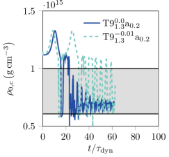
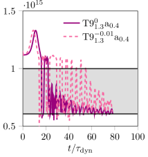
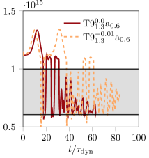
Figure 7: Left panel: Central rest-mass density $\rho_{0,c}$ as a function of time (scaled by the dynamical time $\tau_{\rm dyn}$) for models $\rm T9_{1.3}^{0}a_{0.2}$ with no initial perturbation (solid line) and $\rm T9_{1.3}^{-0.01}a_{0.2}$ with a negative initial pressure perturbation (dashed line). The lower and upper black horizontal lines correspond to the lower and upper bounds of the phase transition, respectively. The gray band corresponds to the phase transition region of the EOS. Center panel: Same as the left panel, but for models $\rm T9_{1.3}^{0}a_{0.4}$ and $\rm T9_{1.3}^{-0.01}a_{0.4}$. Right panel: Same as the left and center panels, but for models $\rm T9_{1.3}^{0}a_{0.6}$ and $\rm T9_{1.3}^{-0.01}a_{0.6}$.

In the case of rotation we focus on the T9 EOS. We consider models with the same central energy density as the non-rotating model of $\epsilon_{\rm c}=$1.3\text{\times}{10}^{15}\text{\,}\mathrm{g}\text{\,}{\mathrm{cm}}^{-3}$$ albeit with different values of the angular momentum. We consider these models both under equilibrium evolution and negative pressure perturbations. We find that all rotating models naturally migrate toward the second-family branch on a dynamical timescale. The rotating models we consider exhibit strong oscillations in the early stages of evolution which are eventually damped as the models tend toward their respective lower-density equilibrium counterparts. As in the non-rotating models discussed in Sec. V.1.3, we find that pressure depletion in rotating models incites strong oscillations. In particular, rotating models under pressure depletion exhibit prolonged oscillations in the rest-mass density when compared to the equilibrium evolution cases. In the following we present the results of our study on rotation, categorizing by the initial perturbation.

V.2.1 Equilibrium evolution

In the left, middle, and right panels of Fig. 7 we show the central rest-mass density for models $\rm T9_{1.3}^{0}a_{0.2}$, $\rm T9_{1.3}^{0}a_{0.4}$, and $\rm T9_{1.3}^{0}a_{0.6}$, respectively, using solid lines. In the case of equilibrium evolution, we find that rotating models exhibit oscillations early in the evolution which are eventually damped as the models settle toward configurations with lower central densities, similar to non-rotating models. The early-time oscillations in rest-mass density for models $\rm T9_{1.3}^{0}a_{0.2}$, $\rm T9_{1.3}^{0}a_{0.4}$, and $\rm T9_{1.3}^{0}a_{0.6}$ are significantly damped (such that the oscillations in $\rho_{\rm c,max}$ are approximately $1-2\%$) within $t\approx 40\tau_{\rm dyn}$, $t\approx 45\tau_{\rm dyn}$, and $t\approx 60\tau_{\rm dyn}$, respectively.

Similar to non-rotating models, the oscillations in rest-mass density are damped on a dynamical timescale. As with non-rotating models, we also find that the rest-mass density presented in Fig. 7 never reaches its pre-bounce value, suggesting that the models are temporarily bouncing to the additional stable configurations with central energy densities between the hadronic and quark phases.

V.2.2 Pressure depletion

The evolution of the central rest-mass density for models $\rm T9_{1.3}^{-0.01}a_{0.2}$, $\rm T9_{1.3}^{-0.01}a_{0.4}$, and $\rm T9_{1.3}^{-0.01}a_{0.6}$ is depicted using dashed lines in the left, center, and right panels of Fig. 7, respectively. Under pressure depletion with rotation, we observe a qualitatively similar evolution to non-rotating cases early on. We observe an initial contraction in the configuration which corresponds to an increasing central rest-mass density. The contraction eventually halts at a maximum and the central region proceeds to bounce between the hadronic and quark phases. For models $\rm T9_{1.3}^{-0.01}a_{0.2}$ and $\rm T9_{1.3}^{-0.01}a_{0.6}$ we observe two consecutive strong bounces early on, as the model returns to the peak rest-mass density once again after the initial contraction. In the late stages of evolution, the oscillations are damped. Despite the early-time strong oscillations for rotating models under pressure depletion, eventually they all tend to settle near their respective lower-density counterparts.

We find that rotating models with negative pressure perturbations tend to undergo strong oscillations of the central region between phases for a prolonged time. For models $\rm T9_{1.3}^{-0.01}a_{0.2}$, $\rm T9_{1.3}^{-0.01}a_{0.4}$ and $\rm T9_{1.3}^{-0.01}a_{0.6}$ we find strong oscillations (where oscillations in $\rho_{\rm c,max}$ are of approximately $50\%$ in amplitude) for the first $t\approx 60\tau_{\rm dyn}$, $t\approx 50\tau_{\rm dyn}$, and $t\approx 80\tau_{\rm dyn}$, respectively. After the stage of strong bouncing, the oscillations are damped. Rotating, radially oscillating compact stars can be potential sources of GWs. We discuss the prospects of detectability for rotating unstable branch hybrid stars in detail in Sec. VI.2.

As in the non-spinning cases, we find that the initial increase in density is large enough for the configurations to reach and exceed the central density of the counterpart stable twin star, but the solution does not settle there. For this reason we also investigate the stability of the stable twin star in App. B. We find that these configurations are dynamically stable (as expected from the turning point theorem), and they do not exhibit large oscillations that would lead them transition to the unstable regime. This suggests, that these stable twin star configurations may need to be reached in a quasi-static way for them to naturally form. However, this could be challenging in the case of a core-collapse supernova or the accretion induced collapse of a white dwarf or even in the case of a white dwarf–neutron star merger, because as the central density increases the hadronic branch is encountered first, and if the density increases further (e.g. due to compression) and crosses over into the phase transition, the EOS will soften, causing the star to undergo collapse until the density becomes high enough for a bounce to take place, and then enter the oscillation cycles we observed here.

Note that the size of the density perturbation influences the timescale over which the early-time strong oscillations persist, as discussed in Sec. V.1.3. As such, the interplay between the strong oscillations incited by pressure depletion and the natural tendency for rotating models to settle to lower central densities may depend sensitively on both the angular momentum of the initial configuration and the size of the initial perturbation. We leave a more in-depth investigation of the interplay between strong quasi-periodic oscillations and rotation for future work.

V.3 Minimum mass instability

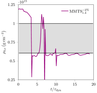
Figure 8: Central rest-mass density $\rho_{0,\rm c}$ for model $\rm MMT9_{1.4}^{-2\%}$ (minimum mass model for the T9 EOS in the case where $2\%$ of the rest mass was removed at the start of the evolution) as a function of time (scaled by the dynamical time $\tau_{\rm dyn}$). The gray band corresponds to the phase transition region, and the lower (upper) black line corresponds to the start (end) of that region.

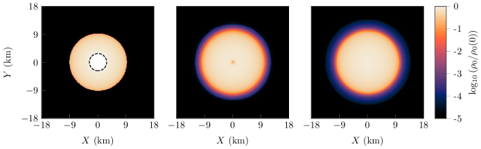
Figure 9: Left panel: Equatorial snapshot of the rest-mass density for model $\rm MMT9_{1.4}^{-2\%}$ (minimum mass model for the T9 EOS in the case where $2\%$ of the rest mass was depleted at the start of evolution) at time $t=0$. The white region surrounded by a dashed black line around the stellar center corresponds to the quark phase. Center panel: Same as the left panel but at time $t\approx 7\tau_{\rm dyn}$. At this stage the model has undergone maximal expansion and a small under-density can be seen to develop at the center. Right panel: Same as the left panel but at time $t\approx 19\tau_{\rm dyn}$ near the end of the evolution. By this stage the model has roughly settled to a lower-density steady state.

Neutron stars near the minimum-mass equilibrium configuration, located on the unstable branch between the stable white-dwarf and stable neutron-star families, undergo a dynamical instability if the mass is lowered below the minimum neutron star mass (e.g. if matter is stripped off the neutron star) Clark and Eardley (1977); Blinnikov et al. (1984); Colpi et al. (1989, 1990); Sumiyoshi et al. (1998). We consider this “minimum-mass instability” in the context of minimum-mass hybrid stars, which are analogously located between the stable neutron star and stable hybrid star families. The neutron star minimum-mass instability sets in for configurations in hydrostatic equilibrium wherein the timescale $\tau_{\beta}$ associated with the electroweak interactions that determines chemical equilibrium is comparable to the dynamical timescale. In cases where $\tau_{\beta}/\tau_{\rm dyn}\gg 1$, the evolution is determined by expansion on a secular timescale, as the configuration has ample time to oscillate about neighboring configurations in hydrostatic equilibrium without undergoing beta decay. On the other hand, if $\tau_{\beta}/\tau_{\rm dyn}\lesssim 1$, the configuration undergoes a dynamical instability which ultimately leads to a spectacular explosion Colpi et al. (1989, 1990); Sumiyoshi et al. (1998); Manukovskii (2010); Yudin et al. (2020). We note that a condition for the base EOSs in this work is chemical equilibrium between the quark and hadronic phases Alvarez-Castillo and Blaschke (2017), and as such the stellar configurations we consider are in cold beta-equilibrium.

For minimum-mass neutron stars, the conditions for the instability may be achieved by mass-stripping, which has the effect of lowering the total mass while keeping the ratio of electrons to baryons fixed. Dynamically, a removal of mass similar to that considered in Colpi et al. (1989, 1990) in the context of hybrid stars may take place in close or eccentric black hole-hybrid star binaries Lattimer and Schramm (1974); Clark and Eardley (1977); East et al. (2012, 2015). To incite an initial perturbation similar to that considered in Colpi et al. (1989, 1990) for the hybrid stars considered in our work, we place a rest-mass density cutoff $\rho_{\rm 0,cutoff}$ on the minimum mass, non-rotating configuration for the T9 EOS. To impose the density cutoff, we set all rest-mass densities below $\rho_{\rm 0,cutoff}$ to the value of the tenuous atmosphere at the start of the simulation. Motivated by findings which show that eccentric or close black hole-neutron star binaries can unbind $\mathcal{O}(10)\%$ or more of the rest mass of one of the binary components during close encounters East et al. (2012, 2015, 2016), we set $\rho_{\rm 0,cutoff}=$1\text{\times}{10}^{14}\text{\,}\mathrm{g}\text{\,}{\mathrm{cm}}^{-3}$$, such that approximately $2\%$ of the initial rest mass is removed. The removal of $2\%$ of the rest mass also ensures that the constraint violations remain small.

In Fig. 8 we show the central rest-mass density for model $\rm MMT9_{1.4}^{-2\%}$ as a function of time. In Fig. 9 we also show equatorial snapshots of the rest-mass density at times $t=0$ (left panel), $t\approx 7t_{\rm dyn}$ (center panel) and $t=19t_{\rm dyn}$ (right panel). We find an initial expansion of the model as the central rest-mass density decreases quickly, and falls below the upper density of the phase transition region, which marks the disappearance of the quark core. At the peak of the expansion, a small under-density momentarily develops at the center of the configuration (shown in the center panel of Fig. 9). The expansion eventually halts and the core partially re-collapses. The core oscillates strongly between the quark and hadronic phases, but eventually settles with a central density lower than that of the original minimum-mass hybrid solution (as shown in the right panel of Fig. 9). In short, we do not observe a runaway expansion of the model analogous to the explosions observed for minimum mass neutron stars. After $t\approx 10\tau_{\rm dyn}$ the model exhibits small ($\sim 5\%$) oscillations in the central rest mass density, close to the central rest-mass density corresponding to the hadronic-branch model with rest mass $M_{0}\approx 0.98M_{0}^{\rm MMT9}$, where $M_{0}^{\rm MMT9}$ is the rest mass of the initial minimum-mass hybrid solution. We find that the rest mass of the initial configuration, after $2\%$ has been removed, is conserved to within 1 part in $10^{5}$.

The evolution of model $\rm MMT9_{1.4}^{-2\%}$ suggests that there is enough binding energy present in the initial minimum-mass model to keep the configuration bound despite the initial expansion. We note that the results presented in this section are an exploratory case-study into the minimum-mass instability for hybrid stars. More studies are required to definitively state that the minimum-mass instability does not lead hybrid stars to explode.

VI Discussion

In this section we discuss the results presented in Sec. V. In particular, we discuss the final state of rotating models in the context of constant rest mass $M_{0}$ sequences and discuss the GW signals associated with the evolution of rotating models which exhibit strong oscillations.

VI.1 Final state in the context of evolutionary sequences

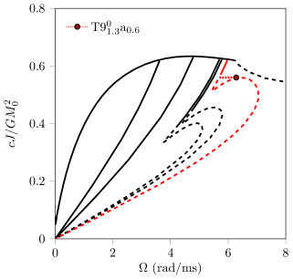
Figure 10: Dimensionless measure of spin, (where $J$ is the total angular momentum and $M_{0}$ is the rest mass) as a function of angular velocity for constant rest mass sequences corresponding to the T9 EOS. The solid (dashed) lines correspond to sequences that only include models with central rest-mass densities below (above) $\rho_{0,\rm tr}^{i}$ as listed in Tab. 1. The red solid and dashed lines correspond to the sequence with rest mass fixed to that of the initial configuration of model $\rm T9_{1.3}^{0}a_{0.6}$. We mark model $\rm T9_{1.3}^{0}a_{0.6}$ with a dark red circle. We also draw a (dotted) line of constant angular momentum representing the expected evolution of model $\rm T9_{1.3}^{0}a_{0.6}$.

A solution space feature associated with the quasi-radial turning-point instability is that unstable branch models near the turning-point may spin up as they lose angular momentum along sequences of constant rest mass $M_{0}$ (so called ‘evolutionary sequences’) Cook et al. (1994a, b). This type of evolution holds in situations where the dynamics happen on a long enough timescale that the models have time to settle into a series of neighboring equilibria as they evolve. However, in marginally stable or unstable cases where the timescale associated with the key features of evolution is shorter, the angular momentum is expected to remain approximately constant as the models spin up Glendenning et al. (1997); Zdunik et al. (2006). For EOSs with strong phase transitions this ‘back-bending’ instability is coupled to the dynamical migration of stars between phases Dimmelmeier et al. (2009). In this section we discuss the evolution and final states for the set of rotating models in our study in the context of their respective evolutionary sequences.

In Fig. 10 we show the dimensionless angular momentum as a function of the angular velocity for several evolutionary sequences corresponding to the T9 EOS. For each sequence, we use solid (dashed) lines to mark the segments where hadronic (hybrid) stars reside, such that their central rest-mass densities fall below (above) $\rho_{0,\rm tr}^{i}$ as listed in Tab. 1. We highlight the evolutionary sequence corresponding to the $\rm T9_{1.3}^{0}a_{0.6}$ model using red lines and mark the corresponding initial configuration with a circle of the same color. In Dimmelmeier et al. (2009) it was observed that marginally stable rotating configurations could be forced toward steady states in the stable hybrid branch by use of density perturbations. It was found that these configurations tend to spin up while keeping a roughly constant angular momentum as they settle into the stable hybrid branch. For the rotating models in our study we find that, even with pressure depletion (which tends to temporarily drive models away from the hadronic branch – the second family), rotating unstable configurations ultimately settle into the stable hadronic branch.

The tendency for the unstable branch models in our study to migrate toward the second-family branch happens on a dynamical timescale. The angular momentum in each of the rotating cases decreases by less than approximately $0.5\%$, consistent with the absence of angular momentum emission in gravitational waves from axisymmetric configurations, and with the level of angular momentum conservation that our code typically achieves. An approximation of the angular velocity using coordinate velocities, i.e., $\Omega=v^{\phi}=d\phi/dt$, reveals that our initial configurations tend to spin down as they settle into the hadronic branch. We note that the such an approximation of the angular velocity is not gauge invariant, and we only use it as a rough indicator to discern whether the angular velocity tends to decrease or increase as the models evolve. The initial configurations discussed in Dimmelmeier et al. (2009) are analogously positioned near the cusp of the red dashed line in Fig. 10 and evolve toward the right on a line of roughly constant angular momentum (for instance, see Fig. 4 of Dimmelmeier et al. (2009)). The $\rm T9_{1.3}^{0}a_{0.6}$ model (represented by the red circle in Fig. 10) instead evolves toward the left roughly along the dotted line corresponding to constant angular momentum. The migration of model $\rm T9_{1.3}^{0}a_{0.6}$ toward the stable hadronic branch happens on a dynamical timescale and we can interpret the configuration as quickly transitioning from its initial state to its final state (after a period of oscillation early on) while keeping $J$ roughly constant, suggesting that the model does not evolve along an evolutionary sequence. The final state of model $\rm T9_{1.3}^{0}a_{0.6}$ should roughly reside at the endpoint of the red dotted line which meets the solid red line (consisting of hadronic models) in Fig. 10. We note that the angular velocity of the model marked by the circle in Fig. 10 is much larger than that of the galactic population of neutron stars Hessels et al. (2006); Papitto et al. (2014). We focus on this model for illustrative purposes, and find that the same general arguments can be made for the models in our study with lower angular velocities.

VI.2 Gravitational waves

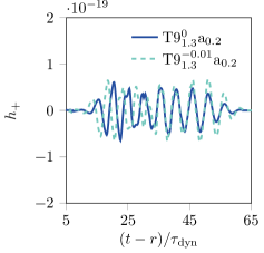
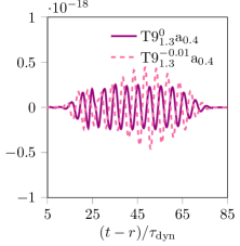
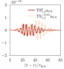
Figure 11: Left panel: Plus polarization of the GW strain $h_{+}$ as a function of time (scaled by the dynamical time $\tau_{\rm dyn}$) for models $\rm T9_{1.3}^{0}a_{0.2}$ (solid line) and $\rm T9_{1.3}^{-0.01}a_{0.2}$ (dashed line) at a distance of $10$ kpc assuming an ideal detector orientation. Center panel: Same as the left panel, but for models $\rm T9_{1.3}^{0}a_{0.4}$ and $\rm T9_{1.3}^{-0.01}a_{0.4}$. Right panel: Same as the left and center panels, but for models $\rm T9_{1.3}^{0}a_{0.6}$ and $\rm T9_{1.3}^{-0.01}a_{0.6}$.

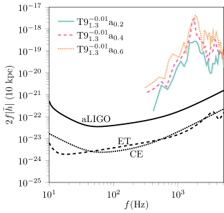
Figure 12: Characteristic strain $h_{\rm c}$ for a source at $10\text{\,}\mathrm{k}\mathrm{p}\mathrm{c}$ for models $\rm T9_{1.3}^{-0.01}a_{0.2}$ (blue solid line), $\rm T9_{1.3}^{-0.01}a_{0.4}$ (magenta dashed line) and $\rm T9_{1.3}^{-0.01}a_{0.6}$ (orange dotted line). We also show the noise curves for future GW observatories including Advanced LIGO (upper line, labeled aLIGO) Einstein Telescope (middle line, labeled ET), and Cosmic Explorer (lower line, labeled CE).

We now turn to the possibility that an unstable branch hybrid configuration could arise as a result of different astrophysical phenomena Takahara and Sato (1988); Gentile et al. (1993); Nakazato et al. (2008); Hempel et al. (2009); Yasutake and Kashiwa (2009); Paschalidis et al. (2009, 2011a, 2011b). Of particular interest is the prospect of white-dwarf accretion-induced collapse or that a WDNS merger results in compression of the neutron star Paschalidis et al. (2009, 2011a, 2011b); Blaschke et al. (2008); Bejger et al. (2011); Drago and Pagliara (2016), which moves part of its core into the phase transition region where the EOS softens and then the neutron star continues to shrink. The subsequent development may be the star dynamically crossing into the unstable twin star regime and undergoing strong oscillations like the ones discussed in this work. Moreover, it may be possible for stable twin stars to dynamically transition into the unstable regime if they are sufficiently close to the minimum mass twin star and are perturbed. Strongly oscillating rotating stars can be a promising source of gravitational waves, and the oscillations driven by the repeated changing of phase in unstable configurations can lead to a characteristic periodicity in the waves. In this section we discuss the gravitational wave radiation associated with the systems we consider as a preliminary consideration of the kinds of gravitational wave signals we may expect from systems that produce hybrid stars.

We generally find that the gravitational radiation associated with the evolution of all rotating models in our study may be detectable only out to the Andromeda galaxy. Depending on the rotation of the system in question, we find evidence of features in the GWs which may point to the evolution of unstable branch hybrid stars as a source. In Fig. 11 we show the plus polarization $h_{+}$ of the GW strain as a function of time for the rotating models in our study, assuming a source at $10\text{\,}\mathrm{k}\mathrm{p}\mathrm{c}$. The solid (dashed) lines in the left, center, and right panels of Fig. 11 correspond to models $\rm T9_{1.3}^{0}a_{0.2}$ ($\rm T9_{1.3}^{-0.01}a_{0.2}$), $\rm T9_{1.3}^{0}a_{0.4}$ ($\rm T9_{1.3}^{-0.01}a_{0.4}$), and $\rm T9_{1.3}^{0}a_{0.6}$ ($\rm T9_{1.3}^{-0.01}a_{0.6}$), respectively. We compute the strain using the FFI method Reisswig et al. (2011) and adopt a low-frequency cutoff $f_{0}=0.2/\tau_{\rm dyn}$ which is lower than the peak frequency observed in the power spectrum of all signals. We focus on the dominant $l=2$, $m=0$ mode and optimal orientation. We find that, as expected, models with stronger rotation produce stronger GWs. Moreover, models with initial negative pressure perturbations produce stronger gravitational waves than cases wherein no perturbation is considered, which is consistent with the stronger oscillations in the rest-mass density observed in cases with pressure depletion.

In Dimmelmeier et al. (2009) it was posited that the dynamical migration of marginally stable hadronic configurations toward the stable hybrid branch (labeled in that study as a ‘mini collapse’) led to a possibly detectable burst of GWs at current and future generation detectors for an event at a distance of $10\text{\,}\mathrm{k}\mathrm{p}\mathrm{c}$. In our cases we do not observe a ‘mini collapse’ scenario (since we don’t start with hadronic configurations), but expect the strength of the GWs to be comparable to the mini collapse scenario of Dimmelmeier et al. (2009) because of the similar size of oscillations within similar mass stars. Thus, we calculate the strain associated with sources at the same distance as Dimmelmeier et al. (2009) for comparison. The strong quasi-periodic oscillations observed throughout the evolution of all rotating models allows for rotating systems which produce gravitational waves with a strong periodicity. The signal associated with these systems builds up strength at roughly constant oscillation frequency as the central region continues to bounce between phases, thereby increasing the detectability of such sources. In Fig. 12 we show the characteristic strain $h_{\rm c}=2f\lvert\tilde{h}\rvert$ (where $\tilde{h}$ is the frequency-domain signal associated with the GWs in Fig. 11) for all rotating models with negative pressure perturbations at a distance of $10\text{\,}\mathrm{k}\mathrm{p}\mathrm{c}$ along with the noise curves of several future GW observatories. The peak frequency for all signals is $f_{\rm peak}\approx$2\text{\,}\mathrm{k}\mathrm{H}\mathrm{z}$$, which falls within a low-sensitivity band for these detectors. We note that the short lived hybrid star remnant observed in Gieg et al. (2019) underwent oscillations which produced GWs with a peak frequency of approximately $3\text{\,}\mathrm{k}\mathrm{H}\mathrm{z}$, which is comparable to our findings. For the distance considered, the GWs for the rotating cases in our study would be detectable by Advanced Ligo (aLIGO) Aasi et al. (2015), Einstein Telescope (ET) Maggiore et al. (2020) and Cosmic Explorer (CE) Reitze et al. (2019). Specifically, we assume a signal-to-noise ratio (SNR) detection threshold of 8 at each detector (see Moore et al. (2015) for the standard definition of SNR we use here). At this SNR threshold, all rotating models in our study are detectable at the three observatories we consider. The detectability increases for models with stronger rotation. We note that near monochromatic GWs may also be expected from oscillating neutron stars. We leave the exploration of how the signals associated with the oscillations of hybrid stars may be distinguishable from those associated with oscillating neutron stars to future work.

Following a GW signal associated with the inspiral of a WDNS, a distinct higher-frequency signal may be observed which could indicate that the remnant underwent strong oscillations between the hadronic and quark phases, similar to the rotating models in our study. We intend to study this scenario in a future work. For sources at a distance of $d_{\rm source}\gtrsim 1$ Mpc, only the models with high spin (models with $a\geq 0.4$) produce detectable signals at all observatories. At this increased distance, models $\rm T9_{1.3}^{0}a_{0.2}$ and $\rm T9_{1.3}^{-0.01}a_{0.2}$ are not detectable at aLIGO but are detectable at ET and CE, while all other rotating models in our study are detectable at the observatories we consider. Thus, third-generation observatories could potentially see such events out to the Andromeda galaxy.

VII Conclusion

Our simulations suggest that unstable branch hybrid configurations tend to migrate toward the hadronic branch – the second family of compact objects – on a dynamical timescale. We find that different types of perturbations drive unstable branch hybrid stars away from the stable hybrid (third-family) branch or incite models to temporarily undergo strong oscillations. Specifically, we find that quasi-radial perturbations induced by positive pressure perturbations drive the stars toward the hadronic (second-family) branch, and that pressure depletion temporarily drives the stars away from the stable hadronic branch. Despite being able to temporarily drive the stars away from settling into a second family configuration, we were not able to force any configurations to settle into a stable third-family model. This is despite the fact that during the evolution the maximum density reaches and exceeds the counterpart stable twin star central density.

In select cases we confirmed that the final states reached by models which tend toward the hadronic branch are consistent with evolutions of the corresponding stable lower-density equilibrium model with the same rest mass as that of the initial configuration. In cases exhibiting small oscillations near the end of the simulations, features of the evolution (such as a decaying amplitude of rest-mass density oscillations) suggest that given enough time, all models will settle into a configuration resembling their respective stable lower-density counterparts. We find that rotating models also naturally tend toward the second-family branch. In rotating cases with pressure depletion, we find that the quasi-periodic oscillations can persist on significant timescales.

After investigating the stability of the stable twin star, we find that these configurations are stable (as expected from the turning point theorem), and they do not exhibit large oscillations that would lead them to transition to the unstable regime. This suggests, that these stable twin star configurations may need to be reached in a quasi-static way for them to naturally form. However, this could be challenging in standard astrophysical scenarios where low mass hybrid stars may be born (such as systems which produce proto-neutron stars Takahara and Sato (1988); Gentile et al. (1993); Nakazato et al. (2008); Hempel et al. (2009); Yasutake and Kashiwa (2009); Most et al. (2019); Weih et al. (2020b), following white dwarf–neutron star mergers Paschalidis et al. (2009, 2011a, 2011b); Blaschke et al. (2008); Bejger et al. (2011); Drago and Pagliara (2016). This is because as the central density increases the hadronic branch is encountered first, and if the density increases further to cross over into the phase transition, the EOS softens, and the star may undergo collapse until the density becomes high enough for a bounce to take place and enter the oscillation cycles we observed here in the case of unstable twin stars. Our findings suggest that if the hadron-quark phase transition is over a large energy density range, it may be difficult to form stable twin stars in nature. If quark matter deconfinement takes place in compact star interiors, it appears that stable hybrid stars more massive than the twin star regime may be preferably formed. This also provides a alternative formation scenario for stable twin stars, whereby a massive hybrid star just above the maximum mass second-family configuration first forms, which subsequently loses mass (e.g., through winds) and enters the stable twin star regime.

Our results show that for sufficiently rapidly spinning stars, these quasi-periodic oscillations the stars may undergo, can produce GW signatures characteristic of sharp phase transition with a large jump in energy density (driven by the softening and stiffening of the EOS over) that can be detectable by ground based observatories as long as these sources are Galactic, but could be detectable out the Andromeda galaxy by third-generation observatories.

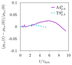
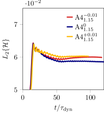
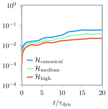
Figure 13: Left panel: Fractional change in the central rest mass density $\rho_{0,\rm c}$ for stable hybrid branch models $\rm A4_{2.0}^{0}$ (magenta solid line) and $\rm T9_{2.3}^{0}$ (blue dashed line). Center panel: $L_{2}$ norm of the Hamiltonian $\mathcal{H}$ constraint for models $\rm A4_{1.15}^{-0.01}$ (red line), $\rm A4_{1.15}^{0}$ (dark blue line), and $\rm A4_{1.15}^{+0.01}$ (yellow line) as a function of time (scaled by the dynamical time $\tau_{\rm dyn}$). The constraints in cases where a pressure perturbation was excited at $t=0$ are comparable to the case of equilibrium evolution. Right panel: $L_{2}$ norm of the Hamiltonian $\mathcal{H}$ constraint as a function of time (scaled by the dynamical time $\tau_{\rm dyn}$) for model $\rm A4_{1.25}^{-0.01}$ at three different grid resolutions. We show results for the canonical (blue line), medium (green line) and high (red line) resolution grids which employ 64, 80, and 96 grid points per hybrid star radius, respectively.

We conclude by pointing out caveats of the present study. Our work provides only some example cases of hybrid hadron quark EOSs that lead to the emergence of a third-family of compact objects. Since the solution space of hybrid stars is EOS-dependent Bozzola et al. (2019), a more extensive study should treat additional EOSs (with varying ranges over which the hadron-to-quark phase transition takes place), different types of perturbations, and probing other parts of the solution space of equilibrium models. For instance, one may consider a wider variety of rotating models to understand the interplay between rotation and their quasi-periodic oscillations. In addition, one can consider the role of rotation and the growth of non-axisymmetric instabilities (see Paschalidis et al. (2018) for a comprehensive review on the types of instabilities relevant to rotating relativistic stars). Finally, differential rotation and magnetic fields can be important following mergers, which significantly affect the dynamics of possible BNS merger remnants Paschalidis et al. (2015); Espino and Paschalidis (2019); Tsokaros et al. (2019); Ruiz et al. (2019); Nathanail (2020); Ruiz et al. (2020) or following a WDNS merger. We leave the investigation of a more extensive solution space on the dynamics and mergers to future studies.

VIII Acknowledgments

It is a pleasure to thank David Blaschke for useful discussions on construction methods for matching hadronic and quark phases. We are grateful to S. L. Shapiro for access to the code that we used to build equilibrium models for relativistic hybrid stars, and to D. Alvarez-Castillo, D. Blaschke and A. Sedrakian for access to the underlying equations of state. PE and VP acknowledge support from NSF Grant PHY-1912619. Simulations were in part performed on the Ocelote and ElGato clusters at the University of Arizona, the Comet cluster at SDSC, and the Stampede2 cluster at TACC through XSEDE grant TG-PHY190020. PE is in part supported by the Marshall Foundation Dissertation Fellowship.

Appendix A Test of stability and resolution study

To test that our modified EOSs allow for stable evolutions, we consider the evolution of a stable branch hybrid star with the A4 EOS with $\epsilon_{c}=$2.0\text{\times}{10}^{15}\text{\,}\mathrm{g}\text{\,}{\mathrm{cm}}^{-3}$$ (model $\rm A4_{2.0}^{0}$) and for the T9 EOS with $\epsilon_{c}=$2.3\text{\times}{10}^{15}\text{\,}\mathrm{g}\text{\,}{\mathrm{cm}}^{-3}$$ (model $\rm T9_{2.3}^{0}$). In the left panel of Fig. 13 we show the fractional change in central rest-mass density for models $\rm A4_{2.0}^{0}$ and $\rm T9_{2.3}^{0}$. We note that these models are not twin stars, and we discuss the stability of stable branch twin stars in App. B. We find that the test models are stable over several dynamical timescales, and showed oscillations in the rest-mass density of at most $2.5\%$ ($1\%$). These tests ensure that the migration of unstable branch hybrid stars toward the hadronic branch are not caused by a lack of stability of hybrid star models using our modified EOSs.

We also consider the effect of the initial pressure perturbations on the constraints during evolution. We focus on the cases of model $\rm A4_{1.15}^{0}$, $\rm A4_{1.15}^{-0.01}$, and $\rm A4_{1.15}^{+0.01}$. In the center panel of Fig. 13 we show the $L_{2}$ norm of the Hamiltonian $\mathcal{H}$ constraint for these models. We find that the constraints are initially small and quickly saturate to approximately constant values. The size and steady state value of the Hamiltonian constraint is only weakly affected by the inclusion of pressure perturbations. This behavior holds for all cases where we include initial perturbations, including the case where we perturb the initial solution with larger or smaller size negative pressure perturbations (see right panel of Fig. 5). As such, our systematic use of changes to the pressure of form Eq. (11) are justified as small perturbations to the initial equilibria that are smaller than the truncation error of the calculation as also illustrated by the convergence plot in the right panel of Fig. 13.

To assess the convergence of our solutions, we perform a resolution study of the $\rm A4_{1.25}^{-0.01}$ model. We consider two additional, higher resolution runs with 1.25 and 1.5 times the resolution of the canonical grid, which we label as our medium- and high-resolution runs, respectively. In the right panel of Fig. 13 we show the $L_{2}$ norm of the Hamiltonian and momentum constraints in the case of the $\rm A4_{1.25}^{-0.01}$ model for our canonical- (blue lines), medium- (green lines), and high- (red lines) resolution grids, which employ at least 64, 80, and 96 grid-points per hybrid star radius, respectively. We find that the salient features of evolution (including the initial contraction of the configuration and subsequent bounce between phases) are generally invariant through higher resolution simulations. Increasing the resolution leads to a slightly later initial bounce and a slightly smaller maximum amplitude of the central rest-mass density, but the evolution of the model is qualitatively invariant after increasing the resolution. We find that the constraints converge to zero with increased grid resolution at approximately second-order, as expected for our numerical scheme.

Appendix B Evolution of stable hybrid twin stars

As an exploration of possible transitions between families of compact stars, we consider the evolution of stable branch hybrid twin stars. We focus on the T9 EOS. We construct a model which is the stable hybrid twin star counterpart to the third entry on Tab. 2. We consider this model under both equilibrium evolution (which we label $\text{T9}_{1.48}^{0}$) and a large positive pressure perturbation of $5\%$ in an effort to drive the model toward a lower density equilibrium (which we label $\text{T9}_{1.48}^{+0.05}$). In Tab. 4, we list some relevant properties of the stable hybrid twin stars we consider.

Table 4: Properties of the stable hybrid models we consider, as a case study of possible dynamical transitions from stable hybrid twin stars to lower density equilibria. For each model, we list the model name, the size of the pressure perturbation parameter $\xi$ (see Eq. (11)), the central energy density $\epsilon_{\rm c}$ and rest-mass density $\rho_{0,\rm c}$ (in units of ${10}^{15}\text{\,}\mathrm{g}\text{\,}{\mathrm{cm}}^{-3}$), the gravitational mass $M$ and rest mass $M_{0}$ (in units of $M_{\odot}$), and the compactness $C$. All models in this case study are built using the T9 EOS.

Model	$\xi$	$\epsilon_{\rm c}$	$\rho_{0,\rm c}$	$M$	$M_{0}$	$C$
$\text{T9}_{1.48}^{0}$	0.00	1.48	1.25	1.53	1.68	0.18
$\text{T9}_{1.48}^{+0.05}$	0.05	1.48	1.25	1.53	1.68	0.18

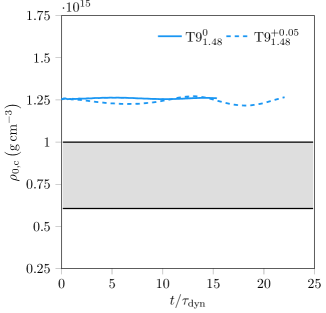
Figure 14: Central rest-mass density $\rho_{0,\rm c}$ as a function of time (scaled by the dynamical time $\tau_{\rm dyn}$) for the models on the stable hybrid branch listed in Tab. 4. In blue we show results for the evolution of models $\text{T9}_{1.48}^{0}$ and $\text{T9}_{1.48}^{+0.05}$ using solid and dashed lines, respectively.

In Fig. 14, we present the evolution of the maximum rest-mass density for the models listed in Tab. 4. The evolution of these models is both an important test of the stability of the stable branch hybrid stars built with our modified EOSs, and serves as a case study of whether stable branch hybrid stars could conceivably migrate to the unstable regime and thereby dynamically transition toward the stable hadronic branch. Our findings suggest that stable branch hybrid stars may not easily transition into the unstable branch. Model $\text{T9}_{1.48}^{0}$ exhibits very small radial oscillations over the simulation time of $t\sim 15\tau_{\rm dyn}$ (shown using the solid blue line in Fig. 14). Model $\text{T9}_{1.48}^{+0.05}$ undergoes much stronger oscillations than $\text{T9}_{1.48}^{0}$, but the central rest-mass density never dips below the value of $\rho_{0,\rm tr}^{f}$ for EOS T9 (see Tab. 1 for the value of $\rho_{0,\rm tr}^{f}$ for this EOS), indicating that the central region remains in the quark phase and that the configuration is oscillating about the initial stable hybrid branch model. Oscillations in the rest-mass density for model $\text{T9}_{1.42}^{+0.05}$ do not grow above $5\%$. The evolution of this model demonstrates that it is stable to radial perturbations, as predicted by the turning-point theorem. In conclusion, this case study demonstrates that it may require strong perturbations for configurations on the stable hybrid twin branch to dynamically transition to the unstable branch and thereby migrate toward lower density equilibria. On the other hand approaching these solutions dynamically from the second family requires strong perturbations whose outcome based on our study of the unstable twin stars is that the stable twin stars are not the preferred end states. Instead the second-family solutions appear to be the natural end states. This suggests that stable twin star solutions may be reached through quasi-static changes from heavier stable hybrid stars that lose mass, e.g., through winds, to end up into the twin star regime. A closer analysis of the dynamics of stable and marginally stable hybrid twin stars under different types of EOS descriptions and perturbations is warranted before we can be conclusively state that stable hybrid twin stars ubiquitously cannot transition to the unstable regime; we leave a more detailed investigation of dynamical transitions away from the stable hybrid branch to future work.

References

- Horowitz (2019) C. Horowitz, Annals Phys. 411, 167992 (2019), arXiv:1911.00411 [astro-ph.HE] .
- Raithel (2019) C. A. Raithel (2019) arXiv:1904.10002 [astro-ph.HE] .
- Baiotti (2019) L. Baiotti, Prog. Part. Nucl. Phys. 109, 103714 (2019), arXiv:1907.08534 [astro-ph.HE] .
- Radice et al. (2020) D. Radice, S. Bernuzzi, and A. Perego, Ann. Rev. Nucl. Part. Sci. 70, 95 (2020), arXiv:2002.03863 [astro-ph.HE] .
- Chatziioannou (2020) K. Chatziioannou, Gen. Rel. Grav. 52, 109 (2020), arXiv:2006.03168 [gr-qc] .
- Baym et al. (2018) G. Baym, T. Hatsuda, T. Kojo, P. D. Powell, Y. Song, and T. Takatsuka, Rept. Prog. Phys. 81, 056902 (2018), arXiv:1707.04966 [astro-ph.HE] .
- Collins and Perry (1975) J. C. Collins and M. J. Perry, Phys. Rev. Lett. 34, 1353 (1975).
- Heiselberg (2000) H. Heiselberg, Physics Reports 328, 237?327 (2000).
- Fukushima and Sasaki (2013) K. Fukushima and C. Sasaki, Prog. Part. Nucl. Phys. 72, 99 (2013), arXiv:1301.6377 [hep-ph] .
- Gerlach (1968) U. H. Gerlach, Phys. Rev. 172, 1325 (1968).
- Kampfer (1981) B. Kampfer, Journal of Physics A Mathematical General 14, L471 (1981).
- Schertler et al. (2000) K. Schertler, C. Greiner, J. Schaffner-Bielich, and M. H. Thoma, Nuclear Physics A 677, 463 (2000), astro-ph/0001467 .
- Glendenning and Kettner (2000) N. K. Glendenning and C. Kettner, A&A 353, L9 (2000), astro-ph/9807155 .
- Alford and Sedrakian (2017) M. Alford and A. Sedrakian, Physical Review Letters 119, 161104 (2017), arXiv:1706.01592 [astro-ph.HE] .
- Ayvazyan et al. (2013) N. S. Ayvazyan, G. Colucci, D. H. Rischke, and A. Sedrakian, A&A 559, A118 (2013), arXiv:1308.3053 [astro-ph.SR] .
- Blaschke et al. (2013) D. Blaschke, D. E. Alvarez-Castillo, and S. Benic, arXiv e-prints (2013), arXiv:1310.3803 [nucl-th] .
- Benić et al. (2015) S. Benić, D. Blaschke, D. E. Alvarez-Castillo, T. Fischer, and S. Typel, A&A 577, A40 (2015), arXiv:1411.2856 [astro-ph.HE] .
- Haensel et al. (2016) P. Haensel, M. Bejger, M. Fortin, and L. Zdunik, European Physical Journal A 52, 59 (2016), arXiv:1601.05368 [astro-ph.HE] .
- Bejger et al. (2017) M. Bejger, D. Blaschke, P. Haensel, J. L. Zdunik, and M. Fortin, A&A 600, A39 (2017), arXiv:1608.07049 [astro-ph.HE] .
- Kaltenborn et al. (2017) M. A. R. Kaltenborn, N.-U. F. Bastian, and D. B. Blaschke, Phys. Rev. D 96, 056024 (2017), arXiv:1701.04400 [astro-ph.HE] .
- Alvarez-Castillo and Blaschke (2017) D. E. Alvarez-Castillo and D. B. Blaschke, Phys. Rev. C 96, 045809 (2017), arXiv:1703.02681 [nucl-th] .
- Abgaryan et al. (2018) V. Abgaryan, D. Alvarez-Castillo, A. Ayriyan, D. Blaschke, and H. Grigorian, Universe 4, 94 (2018), arXiv:1807.08034 [astro-ph.HE] .
- Maslov et al. (2018) K. Maslov, N. Yasutake, A. Ayriyan, D. Blaschke, H. Grigorian, T. Maruyama, T. Tatsumi, and D. N. Voskresensky, arXiv e-prints (2018), arXiv:1812.11889 [nucl-th] .
- Blaschke and Chamel (2018) D. Blaschke and N. Chamel, in Astrophysics and Space Science Library, Astrophysics and Space Science Library, Vol. 457, edited by L. Rezzolla, P. Pizzochero, D. I. Jones, N. Rea, and I. Vidaña (2018) p. 337, arXiv:1803.01836 [nucl-th] .
- Alvarez-Castillo et al. (2019) D. E. Alvarez-Castillo, D. B. Blaschke, A. G. Grunfeld, and V. P. Pagura, Phys. Rev. D 99, 063010 (2019), arXiv:1805.04105 [hep-ph] .
- Paschalidis et al. (2018) V. Paschalidis, K. Yagi, D. Alvarez-Castillo, D. B. Blaschke, and A. Sedrakian, Phys. Rev. D97, 084038 (2018), arXiv:1712.00451 [astro-ph.HE] .
- Bejger et al. (2017) M. Bejger, D. Blaschke, P. Haensel, J. L. Zdunik, and M. Fortin, Astronomy and Astrophysics 600, A39 (2017).
- Montana et al. (2019) G. Montana, L. Tolos, M. Hanauske, and L. Rezzolla, Phys. Rev. D 99, 103009 (2019), arXiv:1811.10929 [astro-ph.HE] .
- Bozzola et al. (2019) G. Bozzola, P. L. Espino, C. D. Lewin, and V. Paschalidis, (2019), arXiv:1905.00028 [astro-ph.HE] .
- Irving et al. (2019) B. Irving, T. Kl hn, P. Jaikumar, M. Salinas, and W. Wei, Universe 5, 193 (2019).
- Bauswein et al. (2020) A. Bauswein, S. Blacker, V. Vijayan, N. Stergioulas, K. Chatziioannou, J. A. Clark, N.-U. F. Bastian, D. B. Blaschke, M. Cierniak, and T. Fischer, (2020), arXiv:2004.00846 [astro-ph.HE] .
- Chatziioannou and Han (2020) K. Chatziioannou and S. Han, Phys. Rev. D 101, 044019 (2020).
- Shahrbaf et al. (2020) M. Shahrbaf, D. Blaschke, A. G. Grunfeld, and H. R. Moshfegh, Phys. Rev. C 101, 025807 (2020).
- Abbott et al. (2020) B. P. Abbott, R. Abbott, T. D. Abbott, S. Abraham, F. Acernese, K. Ackley, C. Adams, V. B. Adya, C. Affeldt, M. Agathos, and et al., Classical and Quantum Gravity 37, 045006 (2020).
- Pereira et al. (2020) J. P. Pereira, M. Bejger, N. Andersson, and F. Gittins, “Tidal deformations of hybrid stars with sharp phase transitions and elastic crusts,” (2020), arXiv:2003.10781 [gr-qc] .
- Abbott et al. (2016) B. P. Abbott et al. (LIGO Scientific Collaboration and Virgo Collaboration), Phys. Rev. Lett. 116, 061102 (2016).
- Abbott et al. (2017a) B. P. Abbott et al., Astrophys. J. Lett. 848, L13 (2017a).
- Abbott et al. (2017b) B. P. Abbott et al., Astrophys. J. Lett. 848, L12 (2017b).
- Bauswein et al. (2017) A. Bauswein, O. Just, H.-T. Janka, and N. Stergioulas, Astrophys. J. 850, L34 (2017).
- Shibata et al. (2017) M. Shibata, S. Fujibayashi, K. Hotokezaka, K. Kiuchi, K. Kyutoku, Y. Sekiguchi, and M. Tanaka, Phys. Rev. D96, 123012 (2017), arXiv:1710.07579 [astro-ph.HE] .
- Margalit and Metzger (2017) B. Margalit and B. D. Metzger, The Astrophysical Journal Letters 850, L19 (2017).
- Abbott et al. (2018) B. P. Abbott et al. (Virgo, LIGO Scientific), (2018), arXiv:1805.11581 [gr-qc] .
- De et al. (2018) S. De, D. Finstad, J. M. Lattimer, D. A. Brown, E. Berger, and C. M. Biwer, Physical Review Letters 121 (2018), 10.1103/physrevlett.121.091102.
- Annala et al. (2017) E. Annala, T. Gorda, A. Kurkela, and A. Vuorinen, (2017), arXiv:1711.02644 [astro-ph.HE] .
- Annala et al. (2017) E. Annala, T. Gorda, A. Kurkela, and A. Vuorinen, ArXiv e-prints (2017), arXiv:1711.02644 [astro-ph.HE] .
- Raithel et al. (2018) C. Raithel, F. Ozel, and D. Psaltis, Astrophys. J. 857, L23 (2018), arXiv:1803.07687 [astro-ph.HE] .
- Rezzolla et al. (2018) L. Rezzolla, E. R. Most, and L. R. Weih, The Astrophysical Journal 852, L25 (2018).
- Ruiz et al. (2018) M. Ruiz, S. L. Shapiro, and A. Tsokaros, Phys. Rev. D97, 021501 (2018).
- Radice et al. (2018) D. Radice, A. Perego, K. Hotokezaka, S. A. Fromm, S. Bernuzzi, and L. F. Roberts, Astrophys. J. 869, 130 (2018), arXiv:1809.11161 [astro-ph.HE] .
- Capano et al. (2019) C. D. Capano, I. Tews, S. M. Brown, B. Margalit, S. De, S. Kumar, D. A. Brown, B. Krishnan, and S. Reddy, (2019), 10.1038/s41550-020-1014-6, arXiv:1908.10352 [astro-ph.HE] .
- Lattimer and Steiner (2014) J. M. Lattimer and A. W. Steiner, Astrophys. J. 784, 123 (2014), arXiv:1305.3242 [astro-ph.HE] .
- Ozel et al. (2016) F. Ozel, D. Psaltis, T. Guver, G. Baym, C. Heinke, and S. Guillot, Astrophys. J. 820, 28 (2016), arXiv:1505.05155 [astro-ph.HE] .
- zel and Freire (2016) F. zel and P. Freire, Ann. Rev. Astron. Astrophys. 54, 401 (2016), arXiv:1603.02698 [astro-ph.HE] .
- Miller and Lamb (2016) M. C. Miller and F. K. Lamb, Eur. Phys. J. A 52, 63 (2016), arXiv:1604.03894 [astro-ph.HE] .
- Gendreau et al. (2016) K. C. Gendreau et al., “The neutron star interior composition explorer (nicer): design and development,” (2016).
- Raaijmakers et al. (2019) G. Raaijmakers, T. E. Riley, A. L. Watts, S. K. Greif, S. M. Morsink, K. Hebeler, A. Schwenk, T. Hinderer, S. Nissanke, S. Guillot, Z. Arzoumanian, S. Bogdanov, D. Chakrabarty, K. C. Gendreau, W. C. G. Ho, J. M. Lattimer, R. M. Ludlam, and M. T. Wolff, The Astrophysical Journal 887, L22 (2019).
- Miller et al. (2019) M. C. Miller, F. K. Lamb, A. J. Dittmann, S. Bogdanov, Z. Arzoumanian, K. C. Gendreau, S. Guillot, A. K. Harding, W. C. G. Ho, J. M. Lattimer, R. M. Ludlam, S. Mahmoodifar, S. M. Morsink, P. S. Ray, T. E. Strohmayer, K. S. Wood, T. Enoto, R. Foster, T. Okajima, G. Prigozhin, and Y. Soong, The Astrophysical Journal 887, L24 (2019).
- Bogdanov et al. (2019a) S. Bogdanov, S. Guillot, P. S. Ray, M. T. Wolff, D. Chakrabarty, W. C. G. Ho, M. Kerr, F. K. Lamb, A. Lommen, R. M. Ludlam, R. Milburn, S. Montano, M. C. Miller, M. Baub ck, F. zel, D. Psaltis, R. A. Remillard, T. E. Riley, J. F. Steiner, T. E. Strohmayer, A. L. Watts, K. S. Wood, J. Zeldes, T. Enoto, T. Okajima, J. W. Kellogg, C. Baker, C. B. Markwardt, Z. Arzoumanian, and K. C. Gendreau, The Astrophysical Journal 887, L25 (2019a).
- Bogdanov et al. (2019b) S. Bogdanov, F. K. Lamb, S. Mahmoodifar, M. C. Miller, S. M. Morsink, T. E. Riley, T. E. Strohmayer, A. K. Tung, A. L. Watts, A. J. Dittmann, D. Chakrabarty, S. Guillot, Z. Arzoumanian, and K. C. Gendreau, The Astrophysical Journal 887, L26 (2019b).
- Burgio et al. (2018) G. F. Burgio, A. Drago, G. Pagliara, H.-J. Schulze, and J.-B. Wei, Astrophys. J. 860, 139 (2018).
- Drago and Pagliara (2018) A. Drago and G. Pagliara, Astrophys. J. Lett. 852, L32 (2018), arXiv:1710.02003 [astro-ph.HE] .
- Hanauske and Bovard (2018) M. Hanauske and L. Bovard, Journal of Astrophysics and Astronomy 39, 45 (2018).
- Montaña et al. (2019) G. Montaña, L. Tolós, M. Hanauske, and L. Rezzolla, Phys. Rev. D 99, 103009 (2019), arXiv:1811.10929 [astro-ph.HE] .
- De Pietri et al. (2019) R. De Pietri, A. Drago, A. Feo, G. Pagliara, M. Pasquali, S. Traversi, and G. Wiktorowicz, (2019), arXiv:1904.01545 [astro-ph.HE] .
- Annala et al. (2019) E. Annala, T. Gorda, A. Kurkela, J. N ttil , and A. Vuorinen, (2019), arXiv:1903.09121 [astro-ph.HE] .
- Han and Steiner (2019) S. Han and A. W. Steiner, Physical Review D 99 (2019), 10.1103/physrevd.99.083014.
- Essick et al. (2019) R. Essick, P. Landry, and D. E. Holz, (2019), arXiv:1910.09740 [astro-ph.HE] .
- Lin et al. (2006) L.-M. Lin, K. S. Cheng, M. C. Chu, and W. M. Suen, Astrophys. J. 639, 382 (2006), arXiv:astro-ph/0509447 .
- Abdikamalov et al. (2009) E. B. Abdikamalov, H. Dimmelmeier, L. Rezzolla, and J. C. Miller, Mon. Not. Roy. Astron. Soc. 394, 52 (2009), arXiv:0806.1700 [astro-ph] .
- Dimmelmeier et al. (2009) H. Dimmelmeier, M. Bejger, P. Haensel, and J. Zdunik, Mon. Not. Roy. Astron. Soc. 396, 2269 (2009), arXiv:0901.3819 [astro-ph.SR] .
- Bejger et al. (2009) M. Bejger, H. Dimmelmeier, P. Haensel, and J. Zdunik, in 12th Marcel Grossmann Meeting on General Relativity (2009) pp. 785–787.
- Weih et al. (2020a) L. R. Weih, M. Hanauske, and L. Rezzolla, Phys. Rev. Lett. 124, 171103 (2020a), arXiv:1912.09340 [gr-qc] .
- Most et al. (2019) E. R. Most, L. J. Papenfort, V. Dexheimer, M. Hanauske, S. Schramm, H. Stoecker, and L. Rezzolla, Phys. Rev. Lett. 122, 061101 (2019), arXiv:1807.03684 [astro-ph.HE] .
- Hanauske et al. (2018) M. Hanauske, Z. S. Yilmaz, C. Mitropoulos, L. Rezzolla, and H. St cker, EPJ Web Conf. 171, 20004 (2018).
- Most et al. (2020) E. R. Most, L. J. Papenfort, V. Dexheimer, M. Hanauske, H. St cker, and L. Rezzolla, Eur. Phys. J. A 56, 59 (2020), arXiv:1910.13893 [astro-ph.HE] .
- Dexheimer et al. (2019) V. Dexheimer, C. Constantinou, E. R. Most, L. J. Papenfort, M. Hanauske, S. Schramm, H. Stoecker, and L. Rezzolla, Universe 5, 129 (2019), arXiv:1905.12658 [nucl-th] .
- Bauswein et al. (2019) A. Bauswein, N.-U. F. Bastian, D. B. Blaschke, K. Chatziioannou, J. A. Clark, T. Fischer, and M. Oertel, Phys. Rev. Lett. 122, 061102 (2019).
- Bucciantini et al. (2019) N. Bucciantini, A. Drago, G. Pagliara, and S. Traversi, “Formation and evaporation of strangelets during the merger of two compact stars,” (2019), arXiv:1908.02501 [astro-ph.HE] .
- Gieg et al. (2019) H. Gieg, T. Dietrich, and M. Ujevic, Particles 2, 365 (2019), arXiv:1908.03135 [gr-qc] .
- Weih et al. (2020b) L. R. Weih, M. Hanauske, and L. Rezzolla, Physical Review Letters 124 (2020b), 10.1103/physrevlett.124.171103.
- Sorkin (1981) R. Sorkin, Astrophys. J. 249, 254 (1981).
- Friedman et al. (1988) J. L. Friedman, J. R. Ipser, and R. D. Sorkin, Astrophys. J. 325, 722 (1988).
- Schiffrin and Wald (2014) J. S. Schiffrin and R. M. Wald, Class. Quant. Grav. 31, 035024 (2014), arXiv:1310.5117 [gr-qc] .
- Prabhu et al. (2016) K. Prabhu, J. S. Schiffrin, and R. M. Wald, Class. Quant. Grav. 33, 185007 (2016), arXiv:1606.00859 [gr-qc] .
- Shapiro and Teukolsky (1983) S. L. Shapiro and S. A. Teukolsky, Research supported by the National Science Foundation. New York, Wiley-Interscience, 1983, 663 p. (1983).
- Takahara and Sato (1988) M. Takahara and K. Sato, Prog. Theor. Phys. 80, 861 (1988).
- Gentile et al. (1993) N. Gentile, M. Aufderheide, G. Mathews, F. Swesty, and G. Fuller, Astrophys. J. 414, 701 (1993).
- Nakazato et al. (2008) K. Nakazato, K. Sumiyoshi, and S. Yamada, Phys. Rev. D 77, 103006 (2008), arXiv:0804.0661 [astro-ph] .
- Hempel et al. (2009) M. Hempel, G. Pagliara, and J. Schaffner-Bielich, Physical Review D 80 (2009), 10.1103/physrevd.80.125014.
- Yasutake and Kashiwa (2009) N. Yasutake and K. Kashiwa, Phys. Rev. D 79, 043012 (2009), arXiv:0902.0111 [astro-ph.HE] .
- Paschalidis et al. (2009) V. Paschalidis, M. MacLeod, T. W. Baumgarte, and S. L. Shapiro, Phys. Rev. D 80, 024006 (2009), arXiv:0910.5719 [astro-ph.HE] .
- Paschalidis et al. (2011a) V. Paschalidis, Z. Etienne, Y. T. Liu, and S. L. Shapiro, Phys. Rev. D 83, 064002 (2011a), arXiv:1009.4932 [astro-ph.HE] .
- Paschalidis et al. (2011b) V. Paschalidis, Y. T. Liu, Z. Etienne, and S. L. Shapiro, Phys. Rev. D 84, 104032 (2011b), arXiv:1109.5177 [astro-ph.HE] .
- Blaschke et al. (2008) D. Blaschke, G. Poghosyan, and H. Grigorian, AIP Conf. Proc. 1068, 191 (2008), arXiv:0809.2309 [astro-ph] .
- Bejger et al. (2011) M. Bejger, J. L. Zdunik, P. Haensel, and M. Fortin, Astron. Astrophys. 536, A92 (2011), arXiv:1109.1179 [astro-ph.HE] .
- Drago and Pagliara (2016) A. Drago and G. Pagliara, Eur. Phys. J. A 52, 41 (2016), arXiv:1509.02134 [astro-ph.SR] .
- Alvarez-Castillo et al. (2019) D. E. Alvarez-Castillo, J. Antoniadis, A. Ayriyan, D. Blaschke, V. Danchev, H. Grigorian, N. K. Largani, and F. Weber, Astron. Nachr. 340, 878 (2019), arXiv:1912.08782 [astro-ph.HE] .
- Clark and Eardley (1977) J. P. A. Clark and D. M. Eardley, Astrophys. J. 215, 311 (1977).
- Blinnikov et al. (1984) S. I. Blinnikov, I. D. Novikov, T. V. Perevodchikova, and A. G. Polnarev, Soviet Astronomy Letters 10, 177 (1984), arXiv:1808.05287 [astro-ph.HE] .
- Colpi et al. (1989) M. Colpi, S. L. Shapiro, and S. A. Teukolsky, Astrophys. J. 339, 318 (1989).
- Colpi et al. (1990) M. Colpi, S. Shapiro, and S. Teukolsky, (1990).
- Sumiyoshi et al. (1998) K. Sumiyoshi, S. Yamada, H. Suzuki, and W. Hillebrandt, A&A 334, 159 (1998), arXiv:astro-ph/9707230 [astro-ph] .
- Cook et al. (1992) G. Cook, S. Shapiro, and S. Teukolsky, Astrophys. J. 398, 203 (1992).
- Cook et al. (1994a) G. Cook, S. Shapiro, and S. Teukolsky, Astrophys. J. 422, 227 (1994a).
- Cook et al. (1994b) G. Cook, S. Shapiro, and S. Teukolsky, Astrophys. J. 424, 823 (1994b).
- Colucci and Sedrakian (2013) G. Colucci and A. Sedrakian, Phys. Rev. C87, 055806 (2013), arXiv:1302.6925 [nucl-th] .
- Witten (1984) E. Witten, Phys. Rev. D 30, 272 (1984).
- Haensel et al. (1986) P. Haensel, J. L. Zdunik, and R. Schaefer, A&A 160, 121 (1986).
- Alcock et al. (1986) C. Alcock, E. Farhi, and A. Olinto, Astrophys. J. 310, 261 (1986).
- Zdunik (2000) J. L. Zdunik, A&A 359, 311 (2000), astro-ph/0004375 .
- Font et al. (1994) J. A. Font, J. M. Ibanez, A. Marquina, and J. M. Marti, A&A 282, 304 (1994).
- Bertil and Heinz-Otto Kreiss (2013) G. Bertil and J. O. Heinz-Otto Kreiss, Time-Dependent Problems and Difference Methods, 2nd Edition (Wiley, 2013).
- Glendenning (1992) N. K. Glendenning, Phys. Rev. D 46, 1274 (1992).
- Maslov et al. (2019) K. Maslov, N. Yasutake, A. Ayriyan, D. Blaschke, H. Grigorian, T. Maruyama, T. Tatsumi, and D. Voskresensky, Phys. Rev. C 100, 025802 (2019), arXiv:1812.11889 [nucl-th] .
- Colpi et al. (1993) M. Colpi, S. L. Shapiro, and S. A. Teukolsky, Astrophys. J. 414, 717 (1993).
- Douchin and Haensel (2001) F. Douchin and P. Haensel, Astronomy and Astrophysics 380, 151?167 (2001).
- Read et al. (2009) J. S. Read, B. D. Lackey, B. J. Owen, and J. L. Friedman, Phys. Rev. D 79, 124032 (2009).
- Paschalidis and Stergioulas (2017) V. Paschalidis and N. Stergioulas, Living Rev. Rel. 20, 7 (2017), arXiv:1612.03050 [astro-ph.HE] .
- Bhattacharyya et al. (2010) A. Bhattacharyya, I. N. Mishustin, and W. Greiner, Journal of Physics G: Nuclear and Particle Physics 37, 025201 (2010).
- Yasutake et al. (2011) N. Yasutake, G. F. Burgio, and H. J. Schulze, Physics of Atomic Nuclei 74, 1502?1507 (2011).
- Duez et al. (2005) M. D. Duez, Y. T. Liu, S. L. Shapiro, and B. C. Stephens, Phys. Rev. D72, 024029 (2005), arXiv:astro-ph/0503421 [astro-ph] .
- Etienne et al. (2010a) Z. B. Etienne, Y. T. Liu, and S. L. Shapiro, Phys. Rev. D 82, 084031 (2010a).
- Etienne et al. (2015) Z. B. Etienne, V. Paschalidis, R. Haas, P. Moesta, and S. L. Shapiro, Class. Quant. Grav. 32, 175009 (2015), arXiv:1501.07276 [astro-ph.HE] .
- Allen et al. (2001) G. Allen, D. Angulo, I. T. Foster, G. Lanfermann, C. Liu, T. Radke, E. Seidel, and J. Shalf, CoRR cs.DC/0108001 (2001).
- Schnetter et al. (2004) E. Schnetter, S. H. Hawley, and I. Hawke, Class. Quant. Grav. 21, 1465 (2004), arXiv:gr-qc/0310042 [gr-qc] .
- Schnetter et al. (2006) E. Schnetter, P. Diener, E. N. Dorband, and M. Tiglio, Class. Quant. Grav. 23, S553 (2006), arXiv:gr-qc/0602104 [gr-qc] .
- Shibata and Nakamura (1995) M. Shibata and T. Nakamura, Phys. Rev. D52, 5428 (1995).
- Baumgarte and Shapiro (1999) T. W. Baumgarte and S. L. Shapiro, Phys. Rev. D59, 024007 (1999), arXiv:gr-qc/9810065 [gr-qc] .
- Bona et al. (1995) C. Bona, J. Masso, E. Seidel, and J. Stela, Phys. Rev. Lett. 75, 600 (1995), arXiv:gr-qc/9412071 [gr-qc] .
- Alcubierre et al. (2001) M. Alcubierre, B. Bruegmann, D. Pollney, E. Seidel, and R. Takahashi, Phys. Rev. D64, 061501 (2001), arXiv:gr-qc/0104020 [gr-qc] .
- Alcubierre et al. (2003) M. Alcubierre, B. Bruegmann, P. Diener, M. Koppitz, D. Pollney, E. Seidel, and R. Takahashi, Phys. Rev. D67, 084023 (2003), arXiv:gr-qc/0206072 [gr-qc] .
- Etienne et al. (2008) Z. B. Etienne, J. A. Faber, Y. T. Liu, S. L. Shapiro, K. Taniguchi, and T. W. Baumgarte, Phys. Rev. D77, 084002 (2008), arXiv:0712.2460 [astro-ph] .
- Etienne et al. (2010b) Z. B. Etienne, Y. T. Liu, and S. L. Shapiro, Phys.Rev. D82, 084031 (2010b).
- Etienne et al. (2012) Z. B. Etienne, V. Paschalidis, Y. T. Liu, and S. L. Shapiro, Phys.Rev. D85, 024013 (2012).
- Espino and Paschalidis (2019) P. Espino and V. Paschalidis, Phys. Rev. D99, 083017 (2019), arXiv:1901.05479 [astro-ph.HE] .
- Newman and Penrose (1962) E. Newman and R. Penrose, J. Math. Phys. 3, 566 (1962).
- Penrose (1963) R. Penrose, Phys. Rev. Lett. 10, 66 (1963).
- Reisswig et al. (2011) C. Reisswig, C. D. Ott, U. Sperhake, and E. Schnetter, Physical Review D 83 (2011), 10.1103/physrevd.83.064008.
- Bozzola (2021) G. Bozzola, Journal of Open Source Software 6, 3099 (2021).
- Guercilena et al. (2017) F. Guercilena, D. Radice, and L. Rezzolla, Comput. Astrophys. Cosmol. 4, 3 (2017), arXiv:1612.06251 [gr-qc] .
- Manukovskii (2010) K. V. Manukovskii, Astronomy Letters 36, 191 (2010).
- Yudin et al. (2020) A. V. Yudin, T. L. Razinkova, and S. I. Blinnikov, Astronomy Letters 45, 847 (2020), arXiv:2005.04428 [astro-ph.HE] .
- Lattimer and Schramm (1974) J. Lattimer and D. Schramm, Astrophys. J. Lett. 192, L145 (1974).
- East et al. (2012) W. E. East, F. Pretorius, and B. C. Stephens, Physical Review D 85 (2012), 10.1103/physrevd.85.124009.
- East et al. (2015) W. E. East, V. Paschalidis, and F. Pretorius, Astrophys. J. 807, L3 (2015), arXiv:1503.07171 [astro-ph.HE] .
- East et al. (2016) W. E. East, V. Paschalidis, F. Pretorius, and S. L. Shapiro, prd 93, 024011 (2016), arXiv:1511.01093 [astro-ph.HE] .
- Glendenning et al. (1997) N. K. Glendenning, S. Pei, and F. Weber, Phys. Rev. Lett. 79, 1603 (1997).
- Zdunik et al. (2006) J. Zdunik, M. Bejger, P. Haensel, and E. Gourgoulhon, Astron. Astrophys. 450, 747 (2006), arXiv:astro-ph/0509806 .
- Hessels et al. (2006) J. W. T. Hessels, S. M. Ransom, I. H. Stairs, P. C. C. Freire, V. M. Kaspi, and F. Camilo, in American Astronomical Society Meeting Abstracts #207, American Astronomical Society Meeting Abstracts, Vol. 207 (2006) p. 209.07.
- Papitto et al. (2014) A. Papitto, D. F. Torres, N. Rea, and T. M. Tauris, A&A 566, A64 (2014), arXiv:1403.6775 [astro-ph.HE] .
- Aasi et al. (2015) J. Aasi et al. (LIGO Scientific), Class. Quant. Grav. 32, 074001 (2015), arXiv:1411.4547 [gr-qc] .
- Maggiore et al. (2020) M. Maggiore et al., JCAP 03, 050 (2020), arXiv:1912.02622 [astro-ph.CO] .
- Reitze et al. (2019) D. Reitze et al., Bull. Am. Astron. Soc. 51, 035 (2019), arXiv:1907.04833 [astro-ph.IM] .
- Moore et al. (2015) C. J. Moore, R. H. Cole, and C. P. L. Berry, Class. Quant. Grav. 32, 015014 (2015), arXiv:1408.0740 [gr-qc] .
- Paschalidis et al. (2015) V. Paschalidis, W. E. East, F. Pretorius, and S. L. Shapiro, Phys. Rev. D92, 121502 (2015), arXiv:1510.03432 [astro-ph.HE] .
- Tsokaros et al. (2019) A. Tsokaros, M. Ruiz, L. Sun, S. L. Shapiro, and K. Uryū, Phys. Rev. Lett. 123, 231103 (2019), arXiv:1907.03765 [gr-qc] .
- Ruiz et al. (2019) M. Ruiz, A. Tsokaros, V. Paschalidis, and S. L. Shapiro, Phys. Rev. D99, 084032 (2019), arXiv:1902.08636 [astro-ph.HE] .
- Nathanail (2020) A. Nathanail, The Astrophysical Journal 892, 35 (2020).
- Ruiz et al. (2020) M. Ruiz, A. Tsokaros, and S. L. Shapiro, Phys. Rev. D 101, 064042 (2020), arXiv:2001.09153 [astro-ph.HE] .