The Atacama Cosmology Telescope: Microwave Intensity and Polarization Maps
of the Galactic Center

Abstract

We present arcminute-resolution intensity and polarization maps of the Galactic center made with the Atacama Cosmology Telescope. The maps cover a 32 deg² field at 98, 150, and 224 GHz with $|l|\leq 4^{\circ}$, $|b|\leq 2^{\circ}$. We combine these data with Planck observations at similar frequencies to create coadded maps with increased sensitivity at large angular scales. With the coadded maps, we are able to resolve many known features of the Central Molecular Zone (CMZ) in both total intensity and polarization. We map the orientation of the plane-of-sky component of the Galactic magnetic field inferred from the polarization angle in the CMZ, finding significant changes in morphology in the three frequency bands as the underlying dominant emission mechanism changes from synchrotron to dust emission. Selected Galactic center sources, including Sgr A*, the Brick molecular cloud (G0.253+0.016), the Mouse pulsar wind nebula (G359.23-0.82), and the Tornado supernova remnant candidate (G357.7-0.1), are examined in detail. These data illustrate the potential for leveraging ground-based cosmic microwave background polarization experiments for Galactic science.

1 Introduction

Some of the most extreme interstellar environments in the Galaxy are found in the Galactic center (e.g., Battersby et al., 2020). The inner $\sim 500$ pc of the Milky Way is home to the Central Molecular Zone (CMZ), the densest concentration of molecular gas in the Galaxy, with a mean density of $\sim 10^{4}$ cm^-3 (Güsten, 1989; Ferrière et al., 2007). The surface density of dense gas greatly exceeds that found in nearby star-forming molecular clouds, Standard prescriptions predict that the CMZ should be an extremely active site of star formation, and yet the observed star formation rate is low; by some estimates, an order of magnitude or more below predictions (e.g., Longmore et al., 2013; Barnes et al., 2017; Nguyen et al., 2021, and references therein).

The apparently inefficient star formation in the CMZ makes this region an ideal testbed for star formation theories, with many factors proposed to explain the observations. These include the strong magnetic field in the Galactic center (Crutcher et al., 1996; Chuss et al., 2003; Ferrière, 2011), the rate of mass inflow to the CMZ (Sormani & Barnes, 2019), the strength and compressibility of turbulence in the CMZ (Federrath et al., 2017), and the possibility that we are observing a relatively quiescent period between episodic bursts of star formation (Kruijssen et al., 2014; Krumholz & Kruijssen, 2015). Furthermore, the CMZ is in some respects a nearby analog of nuclear rings in other galaxies, including high-redshift starbursts. The Galactic center is thus an opportunity for up-close study of the physics relevant to the cosmic history of star formation (Kruijssen & Longmore, 2013; Ginsburg et al., 2019).

The magnetic field in the vicinity of the Galactic center has long been studied with radio polarimetry (Ferrière, 2009; Morris, 2015). The so-called nonthermal radio filaments – thin strands of radio-frequency emission – were some of the earliest observations to shed light on the magnetic field structure toward the Galactic center. The nonthermal radio filaments are, for the most part, strikingly perpendicular to the Galactic plane, and the intrinsic magnetic field inferred from the Faraday de-rotated polarized synchrotron emission tends to lie parallel to the long axis of these filaments (Morris & Yusef-Zadeh, 1985; Yusef-Zadeh & Morris, 1987a; Lang et al., 1999).

Polarized dust emission provides a complementary means of probing the magnetic field structure in the CMZ. Interstellar dust grains emit partially polarized thermal radiation because they are aspherical and preferentially align their short axes parallel to the ambient magnetic field (Purcell, 1975). The polarization angle of the dust emission is thus a line-of-sight (LOS) integrated probe of the plane-of-sky component of the magnetic field orientation. Polarized dust emission has been measured at high angular resolution in small regions toward a number of CMZ molecular clouds (e.g., Novak et al., 2000, 2003; Chuss et al., 2003; Matthews et al., 2009; Roche et al., 2018). Recently, the balloon-borne experiment PILOT presented a 240 $\mu$m map of the polarized dust emission over the entire CMZ region at $2.2^{\prime}$ resolution (Mangilli et al., 2019), along with comparisons to the lower-resolution 353 GHz polarization data measured by the Planck satellite (Planck Collaboration Int. XIX, 2015).

The Atacama Cosmology Telescope (ACT) measures the polarized microwave sky with higher angular resolution than the Planck satellite and greater sensitivity on small scales. In this paper we present new dedicated maps of the Galactic center in total intensity and linear polarization in three ACT frequency bands. We combine the ACT data with Planck data to augment the map sensitivity on larger angular scales. The frequency coverage of the maps presented here probe a range of physical emission mechanisms, enabling a comprehensive view of the Galactic center environment. In polarization these maps probe both polarized dust and synchrotron emission, and in total intensity the maps additionally show features from free-free emission and molecular line emission from transition frequencies that fall within the ACT passbands. These data illustrate the potential of sensitive cosmic microwave background (CMB) polarization experiments for Galactic science.

We describe the ACT observations in Section 2 and the mapmaking and Planck coadd procedures in Section 3. In Sections 4 and 5, we present the maps in total intensity and polarization, respectively, and discuss derived properties, including emission mechanisms, magnetic field orientation, and polarization fraction. In Section 6, we identify notable Galactic center objects and compare to observations at other frequencies. We conclude in Section 7.

2 Observations

ACT is a 6-meter off-axis Gregorian telescope located at an elevation of 5190 m on Cerro Toco in the Atacama Desert in Chile (Fowler et al., 2007; Thornton et al., 2016). ACT scans the millimeter-wave sky with arcminute resolution, complementary to the full-sky lower angular-resolution measurements from satellite missions such as the Wilkinson Microwave Anisotropy Probe (WMAP; Bennett et al., 2013) and Planck (Planck Collaboration I, 2014).

In 2019, the target ACT observing fields were expanded to include the Galactic center region. Between 2019 June 6 and November 29, a total duration of $\sim 35$ hr of data were taken with three Advanced ACTPol dichroic detector arrays PA4, PA5, and PA6 (Henderson et al., 2016; Ho et al., 2017; Choi et al., 2018), at three frequency bands f090, f150, and f220 centered roughly at 98, 150, and 224 GHz, respectively. The beam full-width-half-maximum (FWHM) at each band is $2.0^{\prime}$, $1.4^{\prime}$, and $1^{\prime}$, respectively. The observation field extends roughly from $-89\degree$ to $-97\degree$ in declination and $-33\degree$ to $-25\degree$ in right ascension. This study focuses specifically on a 32 deg² field near the CMZ with Galactic longitude $|l|\leq 4^{\circ}$ and Galactic latitude $|b|\leq 2^{\circ}$.

In this paper we present the maps made using the nighttime observations only, which constitute roughly two-thirds of the total data collected. The daytime observations are affected by a time-dependent beam deformation due to the heating from the Sun that is challenging to correct for in detailed high-resolution maps, and hence those data are excluded from this analysis. Correcting for this beam deformation will be a subject of future study, and the daytime observations may be included for future versions of these maps.

3 Mapmaking

3.1 Mapmaking with ACT

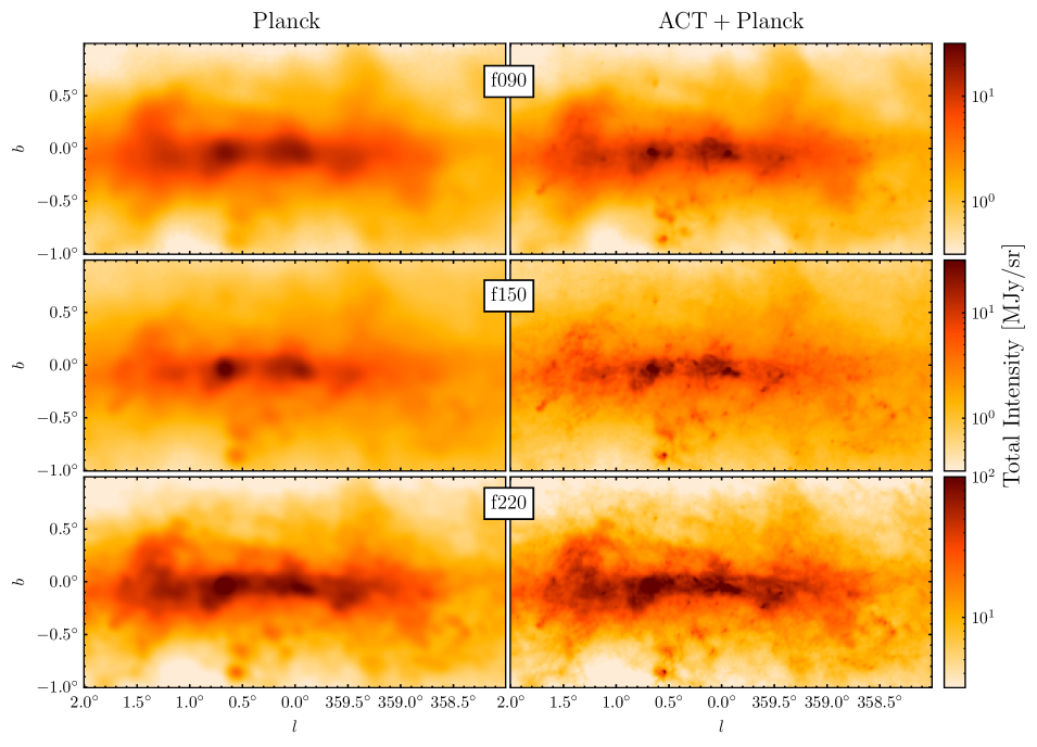
Figure 1: Comparison between Planck-only maps (left column) and ACT+Planck coadded maps (right column) in total intensity. Rows from top to bottom correspond to f090, f150, and f220 respectively. Each map extends from $|l|\leq 2^{\circ}$, $|b|\leq 1^{\circ}$ and is plotted on a logarithmic color scale from 0.3–30 MJy sr^-1 for f090 and f150, and from from 3–100 MJy sr^-1 for f220.

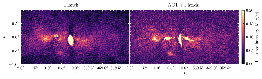
Figure 2: A side-by-side comparison between Planck only (left) and the ACT+Planck coadded (right) for f150 in polarized intensity.

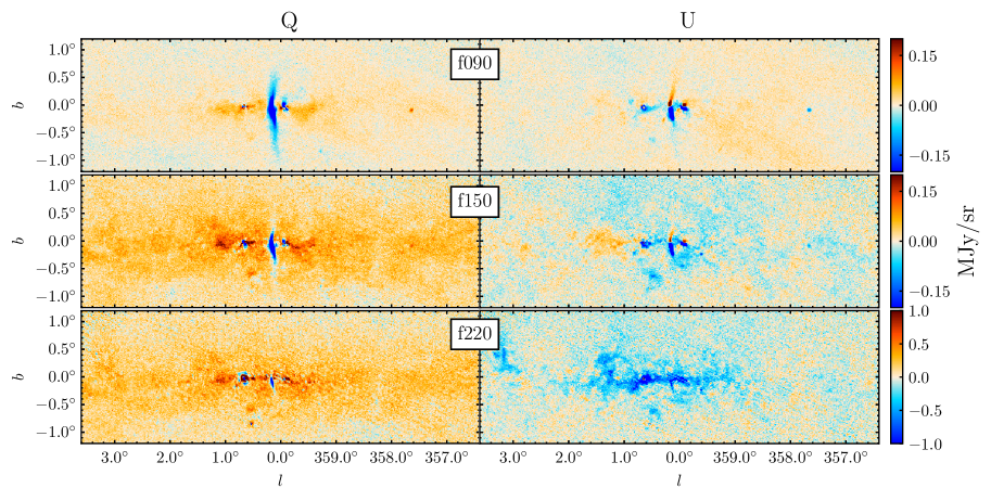
Figure 3: Polarization maps in Stokes $Q$ (left column) and $U$ (right column) in Galactic coordinates and using the IAU polarization convention. Top to bottom are the f090, f150, and f220 maps, respectively.

The instrument records observations in the form of time-ordered data (TOD) in units of $\sim$ 10 minutes. We largely follow the mapmaking pipeline as described in Aiola et al. (2020) with a few key differences, as we briefly summarize below.

First, we cut bad samples affected by glitches in each TOD. To prevent bright sources in the Galactic center region from being mistaken for glitches, we mask sources brighter than 5 mK with a radius of $3^{\prime}$ prior to applying the glitch finder. We also note that this mask is only applied when identifying glitches and not used during mapmaking. Timestreams with outlying statistical properties in terms of noise levels and optical responsiveness are then flagged and removed from the analysis. We further split the dataset into two independent subsets for each frequency band and detector array respectively, resulting in 12 datasets in total. We then obtain the sky maps for each dataset by solving the mapping equation,

$$d=Pm+n,$$ (1)

for a set of Stokes parameters ($I$, $Q$, $U$), where $d$ is the pre-processed time-streamed data, $P$ is the pointing matrix, $m$ is the output map of interest, and $n$ is the noise model. This equation yields a maximum-likelihood solution for $m$ by inverting

$$(P^{T}N^{-1}P)m=P^{T}N^{-1}d,$$ (2)

where $N$ is the detector-detector noise covariance.

There are two notable differences between the pipeline used in this study and that presented in Aiola et al. (2020). First, we have adopted a new calibration method that improves gain stability and reduces biases from thermal contamination as compared to the method in ACT Data Release (DR) 4 (Aiola et al., 2020) (see Appendix A for more details). The second difference relates to the handling of point sources and extended hot regions that are common in the Galactic center region but uncommon in CMB fields. Directly applying the mapmaking pipeline in ACT DR4 leads to stripes around the bright sources caused by model errors as explained in Næss (2019). This happens for two reasons: (1) A pixelated map does not capture the sub-pixel behavior of the sky. These residuals are proportional to the gradient of the signal across a pixel and are often fractionally small. However, if the sky is sufficiently bright, such as in the brightest parts of the Galactic center, they can still end up being large in absolute terms. Since the map $m$ in Equation 1 cannot capture these residuals, the model forces them to be interpreted as part of the noise $n$. (2) The correlated noise model used in the mapmaker induces a nonlocal response to the sub-pixel noise, leading to biases on the scale of the noise correlation length. To avoid this problem, we first identify the regions that source the strongest model errors, namely, the brightest parts of the Galaxy, and then eliminate model errors in these pixels by allocating an extra degree of freedom for each sample that hit them, as described in Næss (2019).

A caveat concerning these maps is that the bright parts of the Galaxy were not masked when building the noise model $N$. The noise model estimator assumes that the time-ordered data is noise dominated ($d\approx n$), and uses this to measure the noise covariance directly from $d$. This breaks down when the telescope scans across the Galactic center, resulting in an overestimate of the noise amplitude especially on smaller scales. This has two consequences: (1) The data are weighted sub-optimally in Equation (2), resulting in slightly higher noise. Since the maps are strongly signal dominated, this can be ignored. (2) Because the noise model is contaminated by the same signal it is applied to, there is a small loss in signal power in the maps; pixels where noise happens to add constructively to the signal have more power in $d$ than in pixels where they partially cancel. Since we use inverse-variance weighting, the latter are up-weighted compared to the former. The size of this effect is limited because the problematically bright regions make up a small fraction of the total samples used to build $N$. We have not measured the precise size of this effect, but estimate it to be $\lesssim 1\%$ based on experience with other high-signal-to-noise (S/N) regions, and hence we expect it to have negligible impact on the interpretation of the maps in this paper. This deficiency will be rectified in the upcoming ACT DR6 maps.

A final known issue requiring mitigation is temperature-to-polarization (T-to-P) leakage. ACT typically scans a given region of the sky both during its rising and setting. As the Galactic center region is at relatively low declination, rising scans and setting scans are poorly cross-linked (for more information on ACT scan strategy see Stevens et al. (2018)). Furthermore, the ACT beam is known to leak T-to-P at the percent level. This beam leakage effect averages down effectively in the nominal CMB maps, which are well cross-linked, but in the Galactic center region the T-to-P leakage is apparent at a $\sim 1$–$2\%$ level that contaminates the polarization maps in the bright Galactic plane. To reduce the contamination from beam leakage, we build a 2D leakage beam model for each dataset using observations of Uranus made in the same observation year (2019), and de-project the expected T-to-P leakage from the polarization maps in each dataset (see Appendix B for more details).

Following these methods, we produced two-way split maps of the Galactic center region at $0.5^{\prime}$ resolution in Plate Carreé (CAR) projection for each frequency band (f090, f150, f220) and detector array (PA4, PA5, PA6) resulting in a total of 12 maps.

3.2 Coadd with Planck

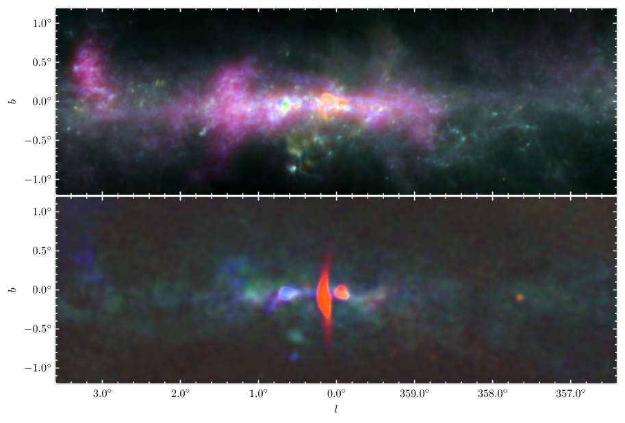
Figure 4: Multifrequency view of the Galactic center region in both total intensity (upper panel) and polarized intensity (lower panel). Red, green, and blue correspond to f090, f150, and f220, respectively. In the upper panel, the maps are scaled logarithmically from 0.2 to 2 MJy sr^-1 for f090, from 0.214 to 2.14 MJy sr^-1 for f150, and from 1.15 to 10.15 MJy sr^-1 for f220. The polarization maps shown in the lower panel are first smoothed with a Gaussian kernel (FWHM$=3.5^{\prime}$) and then scaled linearly from 0 to 1 MJy sr^-1 for f090, to 1.79 MJy sr^-1 for f150, and to 8.2 MJy sr^-1 for f220.

The large angular scales in the ACT maps are affected by atmospheric noise contamination and complicated co-variances at large scales. These modes can be recovered, however, by coadding ACT maps with maps from Planck, which dominate the S/N at large scales $\ell\lesssim 1000$. In particular, we have used a similar algorithm as presented in ACT DR5 (Naess et al., 2020), in combination with the Planck High Frequency Instrument (HFI) maps processed through the NPIPE pipeline (Planck Collaboration Int. LVII, 2020), which are two-way split maps featuring improved noise level and systematic control as compared to the previous Planck data releases.

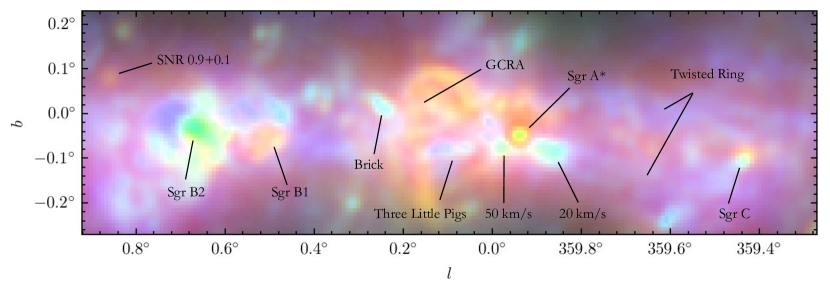
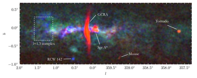
Figure 5: Upper panel: Known radio sources found in the Galactic center region. The background image shows a zoomed-in view of the multifrequency 3-color image presented in the upper panel of Figure 4. Lower panel: Annotations of selected radio and dusty sources in the multifrequency polarized intensity image (presented in the lower panel of Figure 4). Note that we used a smoothing with FWHM=$2^{\prime}$ to make objects more visible.

As the coadding algorithm is presented in detail in Naess et al. (2020), we only briefly summarize the steps and note differences here. First, we re-project the Planck maps and noise models from HEALPix (Górski et al., 2005) projection with $N_{\rm side}=2048$ into the ACT Galactic center observation footprint in CAR projection with $0.5^{\prime}$ pixelization using bi-cubic interpolation. We have used the same passbands as in Naess et al. (2020) and similarly matched the Planck 100 GHz maps with ACT f090 maps, 143 GHz with ACT f150, and 217 GHz with ACT f220. This process assumes that the ACT and Planck passbands are equivalent. We note that this introduces additional scale dependence to the effective band centers (Naess et al., 2020). This is expected to have negligible impact on the results presented here but is relevant for component-separation analysis, which will be the subject of follow-up work.

We then solve for the maximum-likelihood coadded maps using a block-diagonal equation

$$\begin{pmatrix}m_{0}\\ m_{1}\\ \vdots\end{pmatrix}=\begin{pmatrix}B_{0}\\ B_{1}\\ \vdots\end{pmatrix}B_{\rm out}^{-1}m+n,$$ (3)

where $m_{i}$ refers to each individual map, $B_{i}$ refers to its corresponding beam transfer function, and $m$ refers to the final coadded map with a desired beam $B_{\rm out}$, which is the ACT beam in this case. $n$ refers to the map noise, which is assumed to be Gaussian and block diagonal across individual maps, i.e., individual maps have independent noise realizations. Of the noise models presented in Naess et al. (2020), we have adopted the constant correlation noise model, though the choice makes little difference in practice as we are considering only a small patch of sky with close to uniform noise levels. We invert Equation (3) to find a maximum-likelihood solution to the coadded map at f090 and f150, respectively. Because the PA4 array had a poor detector yield over the course of the observation, maps at f220 are treated differently from the other two frequencies. The resulting excess noise in the ACT f220 maps leads to a lack of convergence when solving for a coadded map through a maximum likelihood approach. Therefore, we instead perform a straightforward inverse-variance weighting in Fourier space to obtain the coadded map at f220 (see Appendix C for more details).

One caveat in using the Planck HFI maps is that a cosmic infrared background (CIB) monopole model was deliberately included on a per-frequency basis due to a lack of sensitivity to the absolute emission level. We therefore subtracted the CIB monopole in each coadded map following Table 12 in Planck Collaboration et al. (2020a).

Band	Planck Dataset	ACT Dataset	Total
f090	100 GHz	f090 PA5+PA6	6
f150	143 GHz	f150 PA4+PA5+PA6	8
f220	217 GHz	f220 PA4	4

Table 1: Subsets of maps coadded at each frequency band. All input maps are two-way split maps. The column “total” shows the total number of maps coadded in each band. For example, 6 different maps went into making the f090 coadd map, consisting of two splits from ACT PA4, ACT PA5, and Planck 100 GHz, respectively.

This procedure yields a total of three coadded maps in both temperature and polarization at f090, f150, and f220, as summarized in Table 1. We present a side-by-side comparison between Planck maps and our three coadded maps in total intensity in Figure 1, and a similar comparison for polarized intensity for f150 in Figure 2. It is apparent that the addition of ACT data significantly improves the angular resolution of the maps in both temperature and polarization. The coadded polarization maps are presented in Figure 3 in Galactic coordinates. We use the IAU polarization convention, in which the polarization angle measures 0^∘ toward Galactic North and increases counter-clockwise (Hamaker & Bregman, 1996). The ACT Collaboration has adopted the IAU convention for all ACT data products since DR4. This is in contrast to the COSMO convention (Górski et al., 2005) adopted in, e.g., the Planck data releases, that is related to the IAU convention via a sign flip of Stokes $U$, i.e., $U_{\rm COSMO}=-U_{\rm IAU}$.

A detailed discussion of these maps is presented in Section 4 for total intensity maps and in Section 5 for polarization maps. The final coadded maps have median noise levels of $36\,\mu$K-arcmin at f090, $33\,\mu$K-arcmin at f150, and $270\,\mu$K-arcmin at f220.

4 Total intensity maps

Figure 1 shows the total intensity maps for both Planck-only and the coadded maps for our three frequency bands (f090, f150, f220). Many prominent features that were obscured or unresolved in the Planck maps become apparent with the addition of ACT data, and qualitative changes in map morphology with frequency are evident. The Galactic Center Radio Arc (GCRA), a prominent filament in the Galactic center, is visible at both f090 and f150 near the center of the coadded maps and to a lesser extent at f220, consistent with it being a strong source of synchrotron radiation Paré et al. (2019).

The ACT frequency coverage probes a variety of emission mechanisms, including synchrotron, free-free, thermal dust, and molecular line emission, at different levels in each of the three bands. To better visualize the different structures probed at each frequency band, we combine the coadded maps from three frequency bands into a multicolor image shown in the upper panel of Figure 4. The red, green, and blue image channels represent the f090, f150, and f220 maps, respectively, after appropriate rescaling. The intensity scaling (as detailed in the Figure 4 caption) was chosen to highlight structures in different bands and to make feature identification easier. An annotated zoom-in of the three-color intensity map in Figure 4 is provided in the top panel of Figure 5.

The coherent structures visible in the different colors of Figures 4 and 5 arise from spatial variations in the relative strengths of the various emission mechanisms. The radio spectrum of supernova remnants (SNRs) originates primarily from synchrotron emission (Weiler & Sramek, 1988), and thus objects like the SNR candidate G357.7-0.1 (“the Tornado”) (Milne, 1970) and SNR0.9+0.1 (Helfand & Becker, 1987) appear reddish yellow in Figure 4. Similarly, are strikingly highlighted in this color, consistent with their strong synchrotron emission spectrum. Pulsar wind nebulae (PWN), like the Crab Nebula, also emit highly polarized synchrotron emission with a flat spectral index (Gaensler & Slane, 2006), in contrast to SNRs, which generally emit synchrotron with a slightly lower polarization fraction and a steeper spectrum.

Thermal emission from interstellar dust dominates Galactic emission at far-infrared/submillimeter frequencies. Known molecular molecular clouds like the Brick (G0.253+0.016; e.g., Longmore et al., 2012), the 20 km s^-1 Cloud (G359.889-0.093) and 50 km s^-1 Cloud (G0.070-0.035; e.g., Güsten & Downes, 1980), and the Three Little Pigs (G0.145-0.086, G0.106-0.082, and G0.068-0.075; see, e.g., Battersby et al., 2020, for an overview of these molecular clouds) thus appear bright blue/green in Figure 5.

In general, however, the presence of strong molecular line emission in the CMZ precludes the simple interpretation that low frequencies correspond to synchrotron emission and high frequencies correspond to dust emission. Even in the relatively broad Planck and ACT passbands, line emission can dominate the total intensity in the Galactic center maps. Indeed, Planck Collaboration X (2016) found that 88.6 GHz HCN emission can alone account for up to 23 % of the total intensity in the Planck 100 GHz band in this region. CO(1–0) at 115.3 GHz and CO(2–1) at 230.5 GHz contribute significantly to the observed emission in the Planck 100 and 217 GHz bands, respectively (Planck Collaboration X, 2016), while other lines such as HCO⁺ (89.2 GHz), CS (98.0, 147.0, and 244.9 GHz), ¹³CO(1–0) (110.2 GHz), CN (113.2, 113.5 GHz), H₂CO (140.8 and 218.2 GHz), NO (150.2, 150.5 GHz), SiO (217.1 GHz), SO (219.9 GHz), and ¹³CO(2–1) (220.4 GHz), among others, are also known to be present in the Galactic center (e.g., Liszt & Turner, 1978; Sandqvist, 1989; Kramer et al., 1998; Lang et al., 2002; Takekawa et al., 2014; Pound & Yusef-Zadeh, 2018; Lu et al., 2021; Schuller et al., 2021) and will contribute to the observed emission in the ACT and Planck frequency channels.

The very bright CO(1–0) emission poses a particular challenge for our analysis, as it falls comfortably within the Planck 100 GHz passband but largely outside that of ACT f090 (see Naess et al., 2020, Figure 2). These two frequency channels have been combined without taking the differences in passbands into account, leading to CO(1–0) being emphasized on large Planck-dominated scales in the coadded map, but not on small ACT-dominated scales. This likely explains the haziness of the emission in purple in Figure 4, where the low-frequency channel (red) contains significant CO(1–0) emission in the Planck map but is dominated by other, less prominent emission mechanisms in the ACT map. A quantitative interpretation of the frequency spectra of particular regions in the Galactic center will therefore require careful consideration of bandpass effects, and possibly the use of external spectroscopic data (e.g., Dame et al., 2001; Eden et al., 2020) and/or the CO component maps from Planck (Planck Collaboration X, 2016). Such spectral analysis will be the subject of future work, and for now we urge caution when interpreting the colors in Figure 4 in terms of emission mechanisms or spectral indices.

5 Polarization maps

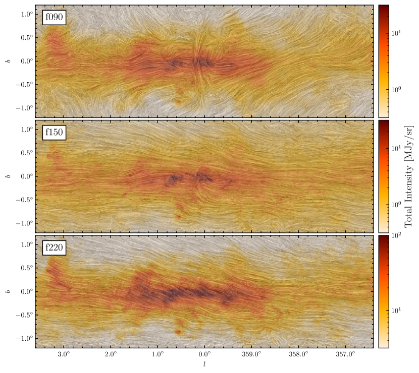
Figure 6: A visualization of magnetic field orientations using line-integral-convolution (LIC) with a $1^{\circ}$ kernel. Contours in the map trace magnetic orientations. Rows represent f090, f150, and f220 respectively. Total intensity maps are shown in the background with the same color scales in Figure 1.

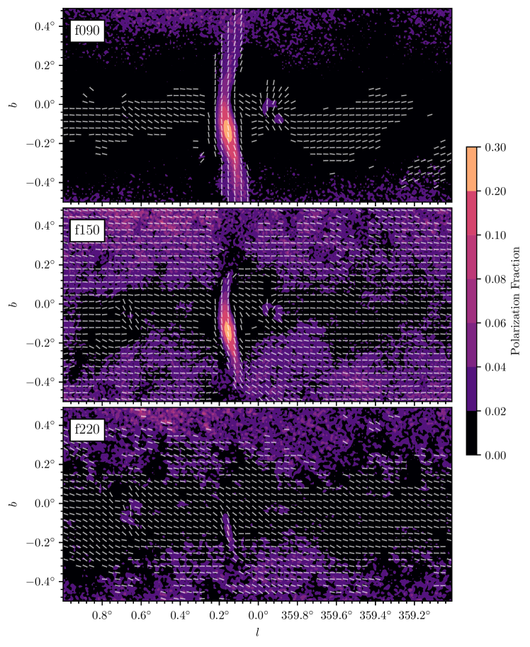
Figure 7: Polarization fractions (background) and magnetic field orientation (line segments) are shown for our three bands (f090, f150, and f220). To estimate the magnetic field orientations, the polarization field is smoothed with a Gaussian kernel FWHM=$2^{\prime}$, and then resampled with a pixel size of $2^{\prime}$. Line segments with large uncertainty in polarization angle $\delta\psi\geq 15^{\circ}$ are masked.

Figure 3 presents the full-resolution Stokes $Q$ and $U$ maps obtained through the mapmaking algorithm at each frequency band. A striking feature of the maps is the strong polarization signal of the GCRA, extending roughly from $b=-0.5^{\circ}$ to $b=0.5^{\circ}$ in both f090 and f150. The signal is weaker in f220, which is dominated by polarized dust emission. Strong polarized signals can be generally seen near the CMZ along the Galactic plane across all frequency bands, with especially prominent polarization features near regions such as Sgr A^∗ and Sgr B2. This suggests that the observed polarization signals are not dominated by diffuse emission along the LOS, but rather by emission directly from the CMZ. Since we are focusing on high S/N regions ($\gtrsim 3$) that are negligibly impacted by debiasing, we do not debias the polarization quantities (Plaszczynski et al., 2014).

To create a three-color polarization image analogous to that in total intensity, we first compute the polarized intensity $P=\sqrt{Q^{2}+U^{2}}$ in each band. We synthesize the three polarized intensity maps into a three-color image using f090, f150, and f220 as the red, green, and blue channels, respectively. The result is shown in the lower panel of Figure 4. The polarized emission has a strikingly different morphology than total intensity (see upper panel of Figure 4). The polarized GCRA stands out distinctively from the background in red, indicating dominance of f090, consistent with the prominence of synchrotron radiation in this region.

One quantity of interest is the polarization angle, defined as

$$\psi=\frac{1}{2}\arctan\left(\frac{U}{Q}\right).$$ (4)

The polarization angle is directly related to the plane-of-sky magnetic field orientation by a 90^∘ rotation. Dust grains tend to align their short axes parallel to the magnetic field, while they radiate photons preferentially polarized parallel to their long axes. The synchrotron polarization angle, or electric vector position angle, is similarly orthogonal to the local magnetic field orientation for optically thin emission. Hence, the magnetic field orientation is orthogonal to the polarization angle in both emission mechanisms. We note, however, that dust and synchrotron emission do not necessarily trace the same magnetic field, as they generally probe different volumes along the LOS. The observed magnetic field morphology at a given frequency depends on the relative contribution of different emission components, which in turn depends on the spatial distribution of dust density versus cosmic ray density and the underlying magnetic field orientation and strength (see Han (2017) for a review).

Figure 6 presents a visualization of the inferred magnetic field orientation in each of our bands using line integral convolution (LIC; Cabral & Leedom, 1993) with a kernel size of $0.5^{\circ}$. Each contour in the map traces the magnetic field orientation. The magnetic field is approximately parallel to the Galactic plane near the CMZ for both f090 and f150, and is noticeably tilted for f220 within the range $|l|\lesssim 1.5^{\circ}$. In particular, within a box of $|l|<1.5^{\circ}$, $|b|<0.15^{\circ}$ we measure the mean polarization angle to have a tilt of $\simeq 20^{\circ}$ with respect to the Galactic plane, consistent with the $\simeq 22^{\circ}$ tilt previously noted by, e.g., PILOT (Mangilli et al., 2019).

The f090 map is noticeably more disordered, with especially prominent features at the GCRA, where the plane-of-sky magnetic field is aligned with the orientation of the arc. This $90^{\circ}$ flip in polarization angle at the GCRA has been observed by the QUIET Collaboration (Ruud et al., 2015) at both 43 GHz and 97 GHz. This orthogonal feature is less prominent at f150 and disappears at f220, as expected from a synchrotron-dominated signal.

The polarization fraction $p=\sqrt{Q^{2}+U^{2}}/I$ in each band is shown in Figure 7. In each panel, we overlay the magnetic field orientation in the CMZ at $2^{\prime}$ resolution. Along the Galactic plane the polarization fraction is generally low, $p\lesssim 2\%$. This is consistent with the previous observations from, e.g., Planck (Planck Collaboration et al., 2020b) and PILOT (Mangilli et al., 2019) that found polarization fractions at the percent level ($\lesssim 1.5\%$) in the Galactic center region. We see coherent magnetic fields even within regions of relatively low polarization fraction, in agreement with both cloud-scale observations and the relatively few wide-area dust polarization measurements, both of which tend to find very ordered magnetic fields (Chuss et al., 2003; Pillai et al., 2015; Mangilli et al., 2019). The large-scale coherence in the inferred magnetic field direction suggests that the polarized emission is dominated by the CMZ. The low polarization fraction could be due to one of several effects, or to a combination of them. Perhaps the most likely is that the magnetic field orientation fluctuates both along the LOS and within the beam smoothing radius, resulting in depolarization. There are so many emitting regions along the LOS in the Galactic disk that small variations in the magnetic field orientation average out in the LOS integration, such that observed deviations from the mean magnetic field orientation are small. We note, however, that simulations of the Galactic magnetic field used to interpret PILOT data suggest that this effect may not be sufficient on its own to account for the entirety of the observed depolarization (Mangilli et al., 2019). Another possibility is that the mean field has a significant LOS component. Because magnetically aligned dust grains spin around their short axes, the net dust emission is more strongly polarized for regions with a predominantly plane-of-sky magnetic field than for regions where the magnetic field is more parallel to the LOS. However, a significant LOS magnetic field component would not be expected to dominate the entirety of the CMZ if the magnetic field has a significant azimuthal component. Finally, it may be that the mean field in the CMZ is itself a product of superimposed, misaligned structures that each have large-scale coherence, e.g., the twisted ring geometry proposed for the distribution of dust density in the CMZ (Molinari et al., 2011). While possible, such a scenario demands great uniformity in the relative total and polarized intensities in each component to avoid dispersion in the observed polarization angles. On balance, we favor a coherent magnetic field in the CMZ dust, with LOS disorder as the primary driver of low polarization fractions, but more detailed modeling of the present data is warranted to assess the relative importance of each of these effects.

6 Notable objects

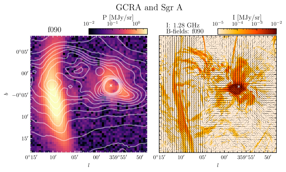
Figure 8: GCRA and Sgr A^∗. The left panel shows the polarized intensity in the region, measured from f090 coadded. Contours show levels of total intensity at f090 with a spacing of 2 MJy sr^-1 up to 30 MJy sr^-1. The right panel shows the inferred magnetic field orientations from the f090 map as line segments in $0.5^{\prime}$ pixelization (full resolution). Segments are shown with varying opacity that scales linearly with the S/N in polarized intensity and saturates when $S/N=3$. In the background we show a radio image of the region from MeerKAT (Heywood et al., 2019) which observes at 1.28 GHz in $6^{\prime\prime}$ pixelization. The expected location of Sgr A^∗ is indicated with a white cross mark in both panels. Note that the MeerKAT image is shown for visualization purposes only, as no primary beam corrections have been applied, and the entire Galactic plane is seen through the primary beam sidelobes. Caution should be taken when interpreting the numerical values in this image (see Heywood et al. (2019) for a detailed discussion).

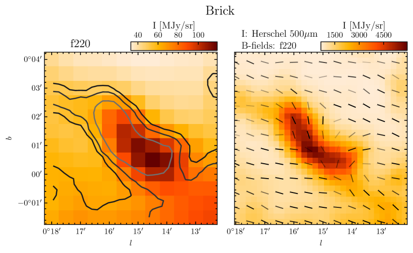
Figure 9: Molecular cloud known as “the Brick”. Left: total intensity measured from ACT+Planck f220 coadd map is plotted in the background. The Herschel $500\,\mu$m measurements (Molinari et al., 2016) are shown as contours indicating 50th, 70th, and 90th percentiles from lighter to darker contours. Right: total intensity measured by Herschel $500\,\mu$m is shown in the background. We show the magnetic field orientation inferred from the f220 map as line segments. Segments are shown with varying opacity that scales linearly with the S/N in polarized intensity and saturates when $S/N=3$.

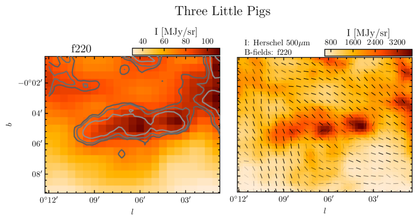
Figure 10: A cloud triad known as “the Three Little Pigs” consisting of G0.145-0.086 (“Straw Cloud”), G0.106-0.082 (“Sticks Cloud”), and G0.068-0.075 (“Stone Cloud”). The data are plotted following Figure 9, with the left panel showing the ACT+Planck f220 map with the Herschel 500 $\mu$m image overlaid as contours (indicating 50th, 70th, and 90th percentiles from lighter to darker colors), and the right panel showing the Herschel 500 $\mu$m map with the magnetic field orientations inferred from the f220 map overlaid as line segments. Segments are shown with varying opacity that scales linearly with the S/N in polarized intensity and saturates when S/N$=3$.

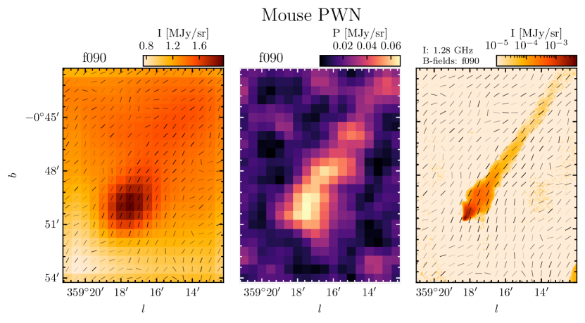
Figure 11: G359.23–0.82 or “the Mouse” is a pulsar wind nebula (PWN) traveling with high velocity ($\sim$300 km s^-1) with respect to ISM, causing a comet-like tail. The left panel shows the total intensity in f090 with magnetic field orientation over-plotted in line segments. Both the background and magnetic field are smoothed to a resolution of $2.2^{\prime}$ to increase the signal-to-noise ratio. Segments are shown with varying opacity that scales linearly with the S/N in polarized intensity and saturates when S/N$=3$. The middle panel shows the polarized intensity in f090 after smoothed to a resolution of $2.2^{\prime}$. The right panel shows a radio image of the region from MeerKAT (Heywood et al., 2019) which observes at 1.28 GHz in $6^{\prime\prime}$ pixelization, with the magnetic field orientation from f090 over-plotted as line segments similar to the leftmost panel.

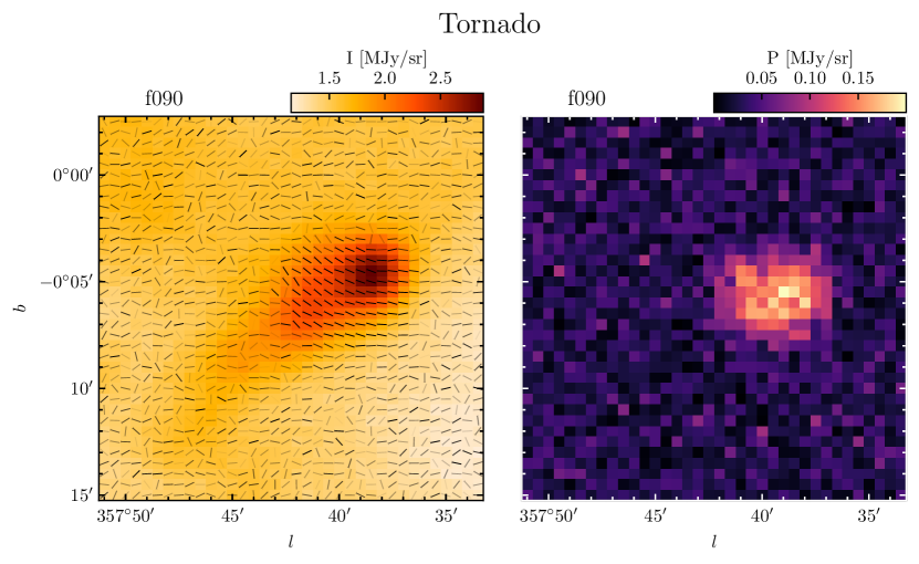
Figure 12: G357.7-0.1, or “the Tornado”, is typically classified as a supernova remnant. The left plot shows the total intensity in its neighborhood in f090 coadded map. Line segments indicate The right plot shows the magnetic field orientations inferred from f090. They are shown with varying opacity that scales linearly with the S/N in polarized intensity and saturates when S/N$=3$. The right panel shows the corresponding polarized intensity map in f090. Both maps are shown at the full resolution from mapmaking ($0.5^{\prime}$).

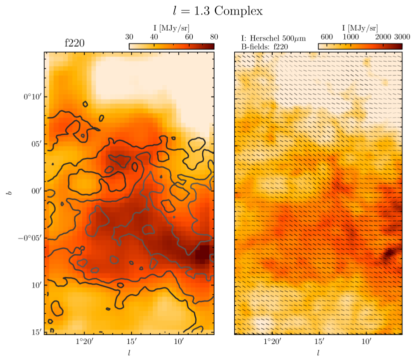
Figure 13: $l=1.3$ molecular complex. The left plot shows the total intensity in f220 (smoothed with FWHM=$1^{\prime}$) with contours indicating the 50th, 70th, 90th percentiles in the Herschel 500 $\mu$m map. The right plot shows the Herschel 500 $\mu$m map with magnetic field orientation inferred from the f220 map as an overlay, after smoothed to a resolution of $1.4^{\prime}$. Segments are shown with varying opacity that scales linearly with the S/N in polarized intensity and saturates when S/N$=3$.

With arcminute resolution in three frequency bands, we detect many known radio and infrared sources, some of which have not been previously observed at ACT frequencies. Although the main focus of this paper is presentation of the Galactic center coadded maps, in this section we demonstrate the fidelity of these maps and their broad potential for different scientific investigations by highlighting select objects. All objects discussed in this section are marked in Figure 5, which includes additional selected radio sources listed in LaRosa et al. (2000) and submillimeter sources from the CMZoom Survey (Battersby et al., 2020) visible in our maps. This list of notable sources is non-exhaustive, and in particular, our maps extend to a wider range in Galactic longitude than either the LaRosa et al. (2000) or Battersby et al. (2020) catalogs.

6.1 Sgr A and GCRA

Sagittarius A (Sgr A) is a complex radio source located at the center of our Galaxy. It consists of Sgr A East, an extended nonthermal source with a radius of $\sim 3^{\prime}$, and a thermal source Sgr A West, which has three-arm spiral morphology and lies within Sgr A East (e.g., Ekers et al., 1983; Yusef-Zadeh & Morris, 1987b; Anantharamaiah et al., 1991). Infrared monitoring of stellar orbits in the vicinity of Sgr A has also revealed the existence of a supermassive black hole Sgr A^∗ that lies within Sgr A West (e.g., Ghez et al., 2008) and acts as the dynamical center of our Galaxy (Backer & Sramek, 1999).

The region of sky surrounding Sgr A^∗ has been the subject of extensive multifrequency observations both in imaging and polarimetry (e.g., Stolovy et al., 1996; Bower & Backer, 1998; Melia et al., 2000; Baganoff et al., 2003; Chuss et al., 2003). Polarized observations in the millimeter bands, in particular, are important for understanding the accretion process near the black hole and associated relativistic emission (e.g., Agol, 2000; Melia et al., 2001). Linear polarization of Sgr A^∗ at millimeter wavelengths was first reported by the Submillimetre Common-User Bolometer Array (SCUBA; Aitken et al., 2000), which they interpret as synchrotron-dominated polarized emission sourced by the gas in the vicinity of the black hole. The observed polarization fraction of Sgr A^∗ is $\sim 3\%$ at 2 mm. Subsequent interferometric imaging surveys (e.g., Macquart et al., 2006; Marrone et al., 2006) measured a $\sim 2\%$ polarization fraction at 3.5 mm, and larger values at higher frequencies. Strong emission centered on Sgr A^∗ is visible in the coadded maps, showing up clearly in the multifrequency image with a yellow color in total intensity (see the upper panel in Figure 5), implying a predominance of synchrotron emission in the region. Its location indicates that the emission is likely dominated by Sgr A^∗ itself instead of the overlapping components in Sgr A that are unresolved with the ACT beam. Regions surrounding Sgr A^∗ are polarized at $2-4\%$ level, as seen in Figure 7 for f090 and f150, and show up as a reddish “blob” in the multifrequency polarimetry (see the lower panel in Figure 5). This may be due to synchrotron emission from the nearby nonthermal filaments within a beam smoothing radius. The polarized emission in the vicinity of Sgr A^∗ has a lower polarization fraction of $\sim 1.5\%$ at all three bands, consistent with the depolarization noted by SCUBA (Aitken et al., 2000) at 2 mm. The slightly lower polarization fraction seen in the ACT data is likely due to a beam depolarization effect from the larger ACT beam ($\sim 2^{\prime}$) in comparison to the SCUBA beam ($\sim 34^{\prime\prime}$ at 2 mm).

In Figure 8 we present a zoom-in view of the region surrounding Sgr A^∗. The left panel shows the polarized signal in f090 overlaid with contours from the total intensity in f090. Strong emission from Sgr A^∗ is seen in total intensity but not in polarization, where the emission is more diffuse and extends $\sim 3^{\prime}$ away from the central source. This is further evidence that the polarized signal in the vicinity of Sgr A^∗ is emitted by the surrounding non-thermal filaments, while the emission from Sgr A^∗ itself is highly depolarized. In the right panel we show the inferred magnetic field orientations from the polarized signal at f090 overlaid on top of a radio image of the same region from MeerKAT (Heywood et al., 2019), which observes at 1.28 GHz with a $6^{\prime\prime}$ beam. The magnetic field morphology inferred from our f090 map closely follows the underlying non-thermal filamentary structure. The morphology is also in broad agreement with previous Caltech Submillimeter Observatory (CSO; Chuss et al., 2003) observations at a wavelength of 350 $\mu$m with a $20^{\prime\prime}$ beam.

Figure 8 also shows the GCRA, a prominent radio feature located at $\sim l=0^{\circ}10^{\prime}$, which consists of a bundle of thin filaments running perpendicular to the Galactic plane (e.g., Yusef-Zadeh & Morris, 1987a; Anantharamaiah et al., 1991). The GCRA is known to be a highly polarized synchrotron source, though its origin is still poorly understood. The strong synchrotron emission implies that free electrons are present in the GCRA and are accelerated to relativistic speeds in the presence of a strong magnetic field in the region. Various models have been proposed to explain the source of electrons and the acceleration mechanism (see, e.g., Serabyn & Morris, 1994, for a review), though the matter is still under debate.

In millimeter bands, the GCRA has previously been detected at 7 mm (Reich et al., 2000), 3 mm (Pound & Yusef-Zadeh, 2018), and 2 mm (Staguhn et al., 2019), which the latter notes was the highest-frequency detection of the GCRA at the time. Polarized emission from the GCRA has also been previously detected at 2 and 3 mm by Culverhouse et al. (2011), and at 3 mm and 7 mm by Ruud et al. (2015). In our coadded maps, GCRA appears in total intensity in both f090 and f150. The associated polarized emission can also be seen clearly in f090 and f150 with polarization fractions reaching $\sim 30\%$. This is considerably higher than the $\sim 10\%$ peak polarization noted by the QUaD Galactic Plane Survey (Culverhouse et al., 2011) at the same frequencies, likely due to the improved angular resolution in our coadded maps ($2^{\prime}$ at f090, $1.4^{\prime}$ at f150) in comparison to Culverhouse et al. (2011) ($5^{\prime}$ at 100 GHz, $3.5^{\prime}$ at 150 GHz). The polarized emission from the southern portion of the GCRA is also visible in f220, which is likely the highest frequency at which this structure is detected to date (note especially the f220 $Q$ map in Figure 3). In addition to being fainter at 220 GHz on account of the falling synchrotron spectrum, the GCRA is also obscured by emission from dust along the LOS. The uniformity of the polarized emission observed in the Arc as seen in Figure 3 implies that a highly ordered magnetic field exists along the Arc that deviates sharply from the large-scale magnetic field geometry (see Figure 6). In particular, the magnetic field orientation inferred from f090 (as seen in the right panel of Figure 8) aligns closely with the filamentary structure perpendicular to the Galactic plane. This is in broad agreement with the morphology observed at 43 GHz and 96 GHz by QUIET with lower angular resolution (Ruud et al., 2015).

6.2 The Brick

G0.253+0.016, also known as “the Brick”, is a dense, massive molecular cloud in the CMZ, and a prominent infrared dark cloud (Carey et al., 1998; Longmore et al., 2012). In the context of understanding the low star formation rate in the Galactic center environment, the Brick is a particularly interesting case study. Despite its high mass $(>10^{5}M_{\sun})$ and density $(>10^{4}~{}\mathrm{cm}^{-3})$, evidence of star formation is nearly absent in the Brick, and thus it may provide an ideal opportunity to study the initial conditions of high-mass star formation (Lis et al., 1994; Longmore et al., 2012; Kauffmann et al., 2013; Mills et al., 2015; Walker et al., 2021). A number of factors have been invoked to explain the dearth of star formation in G0.253+0.016, including solenoidal turbulence driven by strong shear in the CMZ (Federrath et al., 2016; Kruijssen et al., 2019; Dale et al., 2019; Henshaw et al., 2019), or strong cloud-scale magnetic fields ($B\sim\mathrm{mG}$, Pillai et al., 2015).

The Brick stands out at high contrast to the background in the coadded total intensity maps at both 150 and 220 GHz. Our polarization measurements at these frequencies probe the magnetic field structure in the dust toward G0.253+0.016 at $\sim$arcminute scales. These observations complement $20^{\prime\prime}$ resolution polarization data at 350 $\mu$m from the Caltech Submilimeter Observatory (CSO; Dotson et al., 2010; Pillai et al., 2015). We find that the inferred magnetic field orientation is aligned parallel to the long axis of the Brick on the plane of the sky (Figure 9), and the polarization angles are very ordered in this region, in agreement with the CSO data at smaller angular scales. Pillai et al. (2015) use the strong coherence of the magnetic field orientation in the Brick to compare the inferred magnetic field strength to the gas velocity dispersion measured from $\mathrm{N_{2}H^{+}}$ emission (Kauffmann et al., 2013). Those authors find that magnetic fields dominate over turbulence in the Brick. The coherent magnetic field structure in our observations is consistent with the expectation that turbulence in the Brick is sub-Alfvénic at the scales probed by ACT. The ACT polarized emission is brightest at the northern part of the Brick, with a peak polarization fraction of $1.8\%$. The polarized intensity is lower in the southern portion of the cloud, and the SNR on the polarized intensity drops below 3. This depolarization may be due in part to unresolved polarization structure within the ACT beam, and/or to incoherent contributions to the polarized emission along the LOS.

6.3 The Three Little Pigs

The cloud triad G0.145-0.086, G0.106-0.082, and G0.068-0.075 visible in Figure 10 has been dubbed “the Three Little Pigs.” All three clouds have been noted as a set of compact dusty sources in the CMZoom Survey (Battersby et al., 2020), while G0.068-0.075 also appears in the SCUBA-2 Compact Source Catalog (Parsons et al., 2018). As Figure 10 illustrates, each cloud is also apparent in the 500 $\mu$m data from Herschel Infrared Galactic Plane Survey Herschel (Hi-GAL; Molinari et al., 2016). Interestingly, the $3^{\prime\prime}$ resolution 230 GHz observations with the Submillimeter Array as part of the CMZoom Survey have revealed a dearth of substructure in G0.145-0.086 (“Straw Cloud”), somewhat more substructure in G0.106-0.082 (“Sticks Cloud”), and yet more in G0.068-0.075 (“Stone Cloud”).

ACT f220 measurements give a first look at the magnetic field geometry in these clouds at arcminute resolution. The Straw Cloud, perhaps owing to a lower column density or lack of dense substructure, has a magnetic field orientation that deviates little from the large-scale field structure. In contrast, both the Sticks and Stone Clouds have polarization angles in their interiors that are highly misaligned with the large-scale magnetic field. Similar to the depolarization observed toward the Brick, the cancellation of polarized emission from dust in different regions within the cloud and/or other dust along the LOS may explain the low polarized intensities observed, particularly in the Stone Cloud.

6.4 The Mouse

G359.23–0.82, also known as “the Mouse”, is a PWN powered by the young X-ray source PSR J1747–2958 (Predehl & Kulkarni, 1995; Camilo et al., 2002). G359.23–0.82 was originally discovered in radio continuum data from the Very Large Array (VLA), and derives its nickname from its bright compact nebula “head” and extended radio “tail” (Yusef-Zadeh & Bally, 1987). The Mouse is strongly linearly polarized at centimeter wavelengths (Yusef-Zadeh & Gaensler, 2005). Distances to PSR J1747–2958 and the Mouse are uncertain, but they are not at the Galactic center: observations of neutral hydrogen absorption set the maximum distance to G359.23–0.82 at $\sim 5.5$ kpc (Uchida et al., 1992). Gaensler et al. (2004) argue for a distance of $\sim 5$ kpc, a value now commonly adopted (e.g., Klingler et al., 2018). At 5 kpc, the transverse velocity of PSR J1747–2958 is $306\pm 43$ km s^-1 (Hales et al., 2009). The Mouse is a striking example of a bow shock nebula, formed by the interaction of the pulsar with the ambient ISM as it travels at supersonic speeds (e.g., Gaensler & Slane, 2006).

The Mouse is a prominent object in the ACT f090 map, both in total and polarized intensity (Figure 11). In particular, polarized emission is detected significantly across the peak of the Mouse, which is expected for a PWN. Significant polarized emission is also detected along its tail, and exhibits a similar morphology as seen by MeerKAT at 1.28 GHz (Heywood et al., 2019) with a $6^{\prime\prime}$ beam, albeit at lower resolution in the ACT data. The implied magnetic field orientation in the f090 band is roughly parallel to the Mouse’s extended tail, consistent with observations at 3.5 and 6 cm by the VLA (Yusef-Zadeh & Gaensler, 2005). The Mouse is traveling eastward in declination, which is roughly toward the lower left-hand corner of Figure 11.

6.5 The Tornado

G357.7-0.1, “the Tornado,” is typically classified as a SNR, though its unusual properties have prevented a definitive explanation (Gaensler et al., 2003; Chawner et al., 2020). The Tornado has been long observed in radio imaging and polarimetry (e.g., Milne, 1970; Shaver et al., 1985; Law et al., 2008), which consistently show a bright “head” region and a “tail” region roughly $10^{\prime}$ in extent. Recently, mid- and far-infrared dust emission has been detected with Spitzer and Herschel, revealing a large dust reservoir in the head region ($\sim 17$ M_⊙) and consistent with interstellar matter swept up in a supernova blast wave (Chawner et al., 2020). The head of the Tornado has also been detected by Chandra in X-rays without evidence for embedded point sources (Gaensler et al., 2003), lending further credence to its classification as a SNR. However, the provenance of the tail is still unresolved (see Chawner et al., 2020, for a recent discussion).

The Tornado is prominent in the f090 and f150 Stokes $Q$ and $U$ maps, but not f220 (see Figure 3). Likewise, the region stands out in reddish brown in the three-color polarization map (Figure 5). This suggests the prominence of synchrotron emission in this source. A closer examination of the Tornado in the f090 band is presented in Figure 12. Here, we see the extended tail region in total intensity but not in polarization, while the head is prominent in both. This morphology is consistent with 4.9 GHz polarimetric observations by Shaver et al. (1985). The inferred magnetic field at f090 is approximately perpendicular to the extended tail in the eastern side of the Tornado, and is tilted toward the head on the western side. This is also in a broad agreement with the magnetic field morphology noted by (Shaver et al., 1985) at 4.9 GHz. We observe a maximum polarization fraction of the Tornado in f090 of $8.5\%\pm 1\%$, slightly lower than the $\sim 10\%$ observed at 4.9 GHz at significantly higher resolution ($12\times 26^{\prime\prime}$ beam, Shaver et al., 1985). It is likely that much of the difference is due to more beam depolarization in the ACT data.

6.6 $l=1.3$ Complex

The combination of ACT and Planck data used in the coadded maps enables large regions to be mapped with fidelity on both large and small angular scales. Likewise, the high sensitivity of the polarimetry permits mapping of more diffuse regions of molecular clouds, not just bright cores. These capabilities are highlighted in the $20\times 30^{\prime}$ maps of the $l=1.3$ complex in Figure 13.

The $l=1.3$ complex is a large, high-velocity-dispersion molecular cloud complex extending from roughly 1.2–1.6^∘ in Galactic longitude (Bally et al., 1988). The elevated abundance of SiO and high ratio of CO(3–2) to CO(1–0) emission in some clouds within the complex suggest the presence of strong shocks, perhaps from cloud-cloud collisions or supernova explosions (Huettemeister et al., 1998; Oka et al., 2001; Rodriguez-Fernandez et al., 2006; Tanaka et al., 2007; Parsons et al., 2018; Tsujimoto et al., 2021). This complex may sit at the intersection of a dust lane with the nuclear ring, supplying it with material (Huettemeister et al., 1998; Fux, 1999; Rodriguez-Fernandez et al., 2006; Liszt, 2008).

Total emission from the $l=1.3$ in f220 and Herschel 500 $\mu$m (Molinari et al., 2016) is presented in Figure 13, with good morphological correspondence between the two maps. In the right panel, we overlay the f220 magnetic field orientation on the higher resolution Herschel map. While many density structures show clear alignment with the magnetic field orientation, this is not universally observed. The highest intensity regions have comparatively low polarized intensities, suggesting elevated magnetic field disorder or a loss of grain alignment in the densest regions.

7 Summary and future prospects

We have presented new arcminute-resolution maps of the Galactic center region at microwave frequencies by combining data from ACT and Planck. Known radio features appear at high significance in both total intensity and polarization in three frequency bands. The polarization maps provide a frequency-dependent probe of magnetic fields, demonstrating a change in the observed magnetic field morphology as the fractional contributions of synchrotron radiation and thermal dust emission from different regions within the Galactic center along the LOS vary with frequency. With wide-field maps at higher angular resolution, we identified known radio sources and molecular clouds, some of which have not previously been observed in polarization at microwave frequencies. With three frequency bands, our total intensity maps reveal the rich physical environment in the CMZ with spatially varying combinations of different emission mechanisms, including synchrotron, free-free, dust, and molecular line emission in the CMZ. Separation of these emission components will be the subject of a follow-up paper.

The coadded maps produced in this work are now publicly available on the NASA Legacy Archive Microwave Background Data Analysis (LAMBDA; Miller & LAMBDA, 2018). These maps are suitable for tracing magnetic field morphology across the Galactic center region and measuring the total and polarized emission from individual sources. However, caution is urged for multifrequency analyses due to the bandpass mismatch between ACT and Planck that results in a slight scale-dependence of effective band centers for different emission mechanisms. As discussed in Section 4, CO(1-0) emission falls within the Planck 100 GHz passband but not f090, amplifying bandpass mismatch effects in the resulting coadded map.

ACT has continued to observe the Galactic center during 2020, collecting a similar amount of data to that used in this work. In addition, the daytime data from both 2019 and 2020 can, in principle, be corrected for thermal telescope distortions (Aiola et al., 2020), which would again double the total amount of data. Therefore, ACT maps with half the pixel noise variance of those presented here are possible based solely on data that has already been collected. Additionally, we plan to apply the mapping techniques used here to approximately 70 degrees of the Galactic plane covered by ACT from 2019 and 2020. Furthermore, the addition of the low-frequency array to ACT in 2020 (Li et al., 2018; Simon et al., 2018) will also allow us to map the Galactic plane at 27 GHz and 39 GHz, likely yielding new insights on the Galactic center environment.

The next observational step at these frequencies will be the Large Aperture Telescope of the Simons Observatory (Ade et al., 2019), anticipated to see first light in 2023 from the same site in Chile. This new instrument will have the same 6-meter diameter primary as ACT, but with an instrumented focal plane of 5 times larger area (Zhu et al., 2021). The nominal scan strategy will continuously cover the entire sky in the declination range between $+25^{\circ}$ and $-40^{\circ}$, providing coverage of over 100 degrees of the Galactic plane in five frequency bands in both total intensity and polarization. The five-year map noise should improve on ACT by roughly a factor of three. The Galactic center will be observed at higher frequencies by the CCAT-prime project (Choi et al., 2020) and will also be a good target for future balloon-borne instruments, which can achieve sub-arcminute resolution with similar sensitivity at even higher frequencies, e.g., BLAST Observatory (Lowe et al., 2020). By 2030, we can also anticipate data from CMB-S4 (CMB-S4 Collaboration et al., 2016), with an additional map noise improvement by a factor of four. This unrivaled combination of resolution, sky coverage, and sensitivity at microwave frequencies will enable many new inquiries into the properties of the Milky Way.

Appendix A Calibration method

In ACT DR4 (Aiola et al., 2020), the data were calibrated from raw data acquisition units to physical units with

$$d^{\rm pW}=d^{\rm DAQ}\times R_{\rm BS}\times g_{\rm atm}\times f,$$ (A1)

where $d^{\rm pW}$, $d^{\rm DAQ}$ represent detector data in physical unit and data acquisition unit respectively, $R_{\rm BS}$ represents the intrinsic responsivity of each detector measured from the most recent bias step, $g_{\rm atm}$ is the atmospheric correction factor and $f$ represents an optical flatfield. Both $g_{\rm atm}$ and $f$ are estimated from detector responsiveness to the atmospheric signal which is treated as a common mode for all detectors. In the presence of non-atmospheric thermal contamination signatures this approach to estimating the common mode may bias the calibration. Preliminary analyses on the Advanced ACT data collected after 2017 have shown evidences for the presence of such thermal contamination. Hence, the calibration method needs to be updated to account for this bias.

To circumvent the problem, we switch from a common-mode based calibration to a planet based approach, given by

$$d^{\rm pW}=d^{\rm DAQ}\times R_{\rm BS}\times f_{\rm p},$$ (A2)

where we have dropped the atmospheric correction $g_{\rm atm}$. $f_{\rm p}$ now represents an optical flatfield measured from detector responsiveness to emission from Uranus instead of the atmosphere. This leads to an improved calibration model and better gain stability, and this is expected to be the standard calibration method for future data releases of ACT.

One caveat to note is that ACT DR4 (and earlier) maps are calibrated to Planck maps in a final step. This step, however, is missing here due to the preliminary nature of the Advanced ACT data in 2019, but since the Planck calibration is found to be close to the planet calibrations for ACT DR4, and we are using an improved calibration model from DR4, we do not expect this to be a concern and estimate a $O(1\%)$ uncertainty in global gain calibration as a result.

Appendix B Beam leakage correction

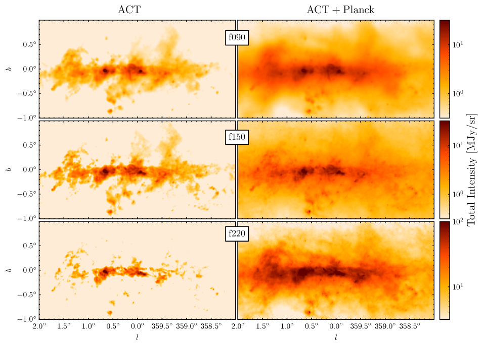
Figure 14:

To reduce the contamination in the polarization maps caused by beam leakage effects, we modeled the observed polarization maps $P_{\rm obs}$ as a sum of a beam-convolved sky map $P_{\rm sky}$ and a leakage component, given by

$$P_{\rm obs}(\mathbf{x})=P_{\rm sky}(\mathbf{x})+\int\frac{d^{2}k}{(2\pi)^{2}}~{}\tilde{T}_{\rm sky}(\mathbf{k})\tilde{B}_{\rm eff}(\mathbf{k})e^{-i\mathbf{k}\cdot\mathbf{x}},$$ (B1)

where the leakage component is a convolution of the beam-convolved temperature map $T_{\rm sky}$ with an effective beam $B_{\rm eff}$ given in Fourier space by

$$\tilde{B}_{\rm eff}(\mathbf{k})\equiv\tilde{B}_{T}^{-1}(\mathbf{k})\tilde{B}_{P}(\mathbf{k})~{}~{}~{}.$$ (B2)

This represents a combination of deconvolving the temperature beam $B_{T}$ and convolving with a leakage beam $B_{P}$. Our strategy is then to build a model of $\tilde{B}_{\rm eff}(\mathbf{k})$, convolve it with the temperature map, and deproject it from the observed polarization maps for each dataset.

As we assumed Uranus signal is unpolarized, any signal we measure in the polarization is a sign of T-to-P leakage. Hence, we modeled $\tilde{B}_{\rm eff}$ using observations of Uranus made in the same observation season, with the following steps:

1. We made Uranus planet maps for each Uranus observation in a source-centered reference frame with the scan direction as the horizontal axis.

2. We reprojected each planet map into the Galactic coordinate system. As the $Q$/$U$ reference frame needs to be rotated depending on the scan directions, and the Galactic center observations consist of two scan directions taken during rising and setting respectively, we accounted for the difference in scan directions by rotating the $Q$/$U$ reference frame for both rising and setting scan directions and performed a weighted average (for each planet map) depending on the total number of rising and setting scans made during Galactic center observations.

3. We stacked all reprojected Uranus maps for each dataset (per frequency band per array) with inverse-variance weighting to obtain estimates of $B_{T}$ and $B_{P}$ for each dataset.

4. We performed a real space cut to remove noise outside a radius of $r_{\rm max}$ in $B_{T}$ and $B_{P}$ for each dataset, then calculated $\tilde{B}_{\rm eff}(\mathbf{k})=\tilde{B}_{P}/\tilde{B}_{T}$ in Fourier space.

5. We further cleaned $\tilde{B}_{\rm eff}(\mathbf{k})$ with a $k$-space cut $k\leq k_{\rm max}$ to get rid of small scale noise in the beam model. We then re-filled the $k$-space outside $k_{\rm max}$ by mirroring the value at $k=k_{\rm max}$ with $\tilde{B}_{\rm eff}(\mathbf{k})|_{k>k_{\rm max}}=\tilde{B}_{\rm eff}(\mathbf{k}~{}k_{\rm max}/k)$. In practice, the details of the extrapolating function make little difference. This specific function is chosen to ensure that the transition at $k=k_{\rm max}$ is smooth, and it extends naturally to infinity.

In Table 2, we listed the choices of $r_{\rm max}$ and $k_{\rm max}$ for each dataset. As a result of these steps, we obtained $\tilde{B}_{\rm eff}(\mathbf{k})$ for each dataset respectively. Treating the coadded temperature map as the “true” sky model $T_{\rm sky}$ at each frequency band, we predicted the expected T-to-P leakage from the derived leakage beam model $\tilde{B}_{\rm eff}(\mathbf{k})$ and subsequently deprojected the expected leakage from each observed map.

array	freq	$r_{\rm max}$	$k_{\rm max}$
PA4	f150	5′	14500
PA4	f220	4′	20000
PA5	f090	8′	10500
PA5	f150	5′	16500
PA6	f090	8′	10500
PA6	f150	5′	16500

Table 2: Parameters used when building a 2D leakage beam model (in step 4 and step 5).

Appendix C Coadded f220 maps

Maps at f220 are much noisier than the two other bands, so using the same coadding pipeline results in a slow convergence. Instead, we adopted a simpler Fourier-based coadding algorithm. Denote the ACT f220 map as $m_{1}$, and Planck 217 GHz map as $m_{2}$. The coadd map $m_{\rm coadd}$ was obtained with a simple inverse-variance coadding as

$$m_{\rm coadd}=\left(N_{1}^{-1}+N_{2}^{-1}\right)^{-1}\left(N_{1}^{-1}m_{1}+N_{2}^{-1}m_{2}\right),$$ (C1)

where $N_{1}$ and $N_{2}$ are noise covariance matrices assumed for ACT and Planck maps respectively. Specifically, we assumed simple Fourier-based noise model with $N_{1}=w_{1}^{2}[1+(\ell/\ell_{\rm knee})^{-\alpha}]$ and $N_{2}=w_{2}^{2}b_{1}/b_{2}$, with $w_{1}=268.97~{}\mu$K^′, $w_{2}=124.22~{}\mu$K^′ the noise levels of ACT and Planck maps respectively, $\ell_{\rm knee}=4000$, and $\alpha=-3$. $b_{1}$ and $b_{2}$ represent the beam model in ACT and Planck respectively, and the factor $b_{1}/b_{2}$ in $N_{2}$ represents the effect of a combination of deconvolution of the Planck beam and convolution with the ACT beam in the Planck noise model. In addition, we further applied a high-pass Butterworth filter in the ACT map with $\ell_{c}=2500$ and $\alpha=-5$ along the two cross-linked scan directions with a width given by the beam FWHM in Fourier space. This helps suppress excess noise along the scan directions. We then applied an additional high-pass Butterworth filter with $\ell_{c}=200$ and $\alpha=-10$ to suppress the large-scale atmospheric noise in the ACT f220 map. Both of these filters are included in the ACT noise model $N_{\ell}$.

The inverse-variance map of the output coadd map was estimated using the same weighted average from Planck inverse-variance map ${\cal N}_{1}^{-1}$ and ACT inverse-variance map ${\cal N}_{2}^{-1}$, given by

$${\cal N}_{\rm coadd}=\overline{c}_{1}^{2}{\cal N}_{1}+\overline{c}_{2}^{2}{\cal N}_{2}$$ (C2)

with $\overline{c}_{1}$, $\overline{c}_{2}$ defined as the $\ell$-space mean of $c_{1,2}\equiv N_{1,2}^{-1}/(N_{1}^{-1}+N_{2}^{-1})$ from $\ell=2500$ to $5000$ where we expect to be dominated by white noise.

References

- Ade et al. (2019) Ade, P., Aguirre, J., Ahmed, Z., et al. 2019, J. Cosmology Astropart. Phys, 2019, 056, doi: 10.1088/1475-7516/2019/02/056
- Agol (2000) Agol, E. 2000, ApJ, 538, L121, doi: 10.1086/312818
- Aiola et al. (2020) Aiola, S., Calabrese, E., Maurin, L., et al. 2020, J. Cosmology Astropart. Phys, 2020, 047, doi: 10.1088/1475-7516/2020/12/047
- Aitken et al. (2000) Aitken, D. K., Greaves, J., Chrysostomou, A., et al. 2000, ApJ, 534, L173, doi: 10.1086/312685
- Anantharamaiah et al. (1991) Anantharamaiah, K. R., Pedlar, A., Ekers, R. D., & Goss, W. M. 1991, MNRAS, 249, 262, doi: 10.1093/mnras/249.2.262
- Backer & Sramek (1999) Backer, D. C., & Sramek, R. A. 1999, ApJ, 524, 805, doi: 10.1086/307857
- Baganoff et al. (2003) Baganoff, F. K., Maeda, Y., Morris, M., et al. 2003, ApJ, 591, 891, doi: 10.1086/375145
- Bally et al. (1991) Bally, J., Casement, S., Goss, W. M., et al. 1991, in Bulletin of the American Astronomical Society, Vol. 23, 890
- Bally et al. (1988) Bally, J., Stark, A. A., Wilson, R. W., & Henkel, C. 1988, ApJ, 324, 223, doi: 10.1086/165891
- Barnes et al. (2017) Barnes, A. T., Longmore, S. N., Battersby, C., et al. 2017, MNRAS, 469, 2263, doi: 10.1093/mnras/stx941
- Battersby et al. (2020) Battersby, C., Keto, E., Walker, D., et al. 2020, ApJS, 249, 35, doi: 10.3847/1538-4365/aba18e
- Bennett et al. (2013) Bennett, C. L., Larson, D., Weiland, J. L., et al. 2013, ApJS, 208, 20, doi: 10.1088/0067-0049/208/2/20
- Bower & Backer (1998) Bower, G. C., & Backer, D. C. 1998, ApJ, 496, L97, doi: 10.1086/311259
- Cabral & Leedom (1993) Cabral, B., & Leedom, L. C. 1993, in Proceedings of the 20th annual conference on Computer graphics and interactive techniques, 263–270
- Camilo et al. (2002) Camilo, F., Manchester, R. N., Gaensler, B. M., & Lorimer, D. R. 2002, ApJ, 579, L25, doi: 10.1086/344832
- Carey et al. (1998) Carey, S. J., Clark, F. O., Egan, M. P., et al. 1998, ApJ, 508, 721, doi: 10.1086/306438
- Chawner et al. (2020) Chawner, H., Howard, A. D. P., Gomez, H. L., et al. 2020, MNRAS, 499, 5665, doi: 10.1093/mnras/staa2925
- Choi et al. (2018) Choi, S. K., Austermann, J., Beall, J. A., et al. 2018, Journal of Low Temperature Physics, 193, 267, doi: 10.1007/s10909-018-1982-4
- Choi et al. (2020) Choi, S. K., Austermann, J., Basu, K., et al. 2020, Journal of Low Temperature Physics, 199, 1089, doi: 10.1007/s10909-020-02428-z
- Chuss et al. (2003) Chuss, D. T., Davidson, J. A., Dotson, J. L., et al. 2003, ApJ, 599, 1116, doi: 10.1086/379538
- CMB-S4 Collaboration et al. (2016) CMB-S4 Collaboration, Abazajian, K. N., Adshead, P., et al. 2016, arXiv e-prints, arXiv:1610.02743. https://arxiv.org/abs/1610.02743
- Crutcher et al. (1996) Crutcher, R. M., Roberts, D. A., Mehringer, D. M., & Troland, T. H. 1996, ApJ, 462, L79, doi: 10.1086/310031
- Culverhouse et al. (2011) Culverhouse, T., Ade, P., Bock, J., et al. 2011, ApJS, 195, 8, doi: 10.1088/0067-0049/195/1/8
- Dale et al. (2019) Dale, J. E., Kruijssen, J. M. D., & Longmore, S. N. 2019, MNRAS, 486, 3307, doi: 10.1093/mnras/stz888
- Dame et al. (2001) Dame, T. M., Hartmann, D., & Thaddeus, P. 2001, ApJ, 547, 792, doi: 10.1086/318388
- Dotson et al. (2010) Dotson, J. L., Vaillancourt, J. E., Kirby, L., et al. 2010, ApJS, 186, 406, doi: 10.1088/0067-0049/186/2/406
- Eden et al. (2020) Eden, D. J., Moore, T. J. T., Currie, M. J., et al. 2020, MNRAS, 498, 5936, doi: 10.1093/mnras/staa2734
- Ekers et al. (1983) Ekers, R. D., van Gorkom, J. H., Schwarz, U. J., & Goss, W. M. 1983, A&A, 122, 143
- Federrath et al. (2016) Federrath, C., Rathborne, J. M., Longmore, S. N., et al. 2016, ApJ, 832, 143, doi: 10.3847/0004-637X/832/2/143
- Federrath et al. (2017) Federrath, C., Rathborne, J. M., Longmore, S. N., et al. 2017, in The Multi-Messenger Astrophysics of the Galactic Centre, ed. R. M. Crocker, S. N. Longmore, & G. V. Bicknell, Vol. 322, 123–128, doi: 10.1017/S1743921316012357
- Ferrière (2009) Ferrière, K. 2009, A&A, 505, 1183, doi: 10.1051/0004-6361/200912617
- Ferrière (2011) Ferrière, K. 2011, in Astrophysical Dynamics: From Stars to Galaxies, ed. N. H. Brummell, A. S. Brun, M. S. Miesch, & Y. Ponty, Vol. 271, 170–178, doi: 10.1017/S1743921311017583
- Ferrière et al. (2007) Ferrière, K., Gillard, W., & Jean, P. 2007, A&A, 467, 611, doi: 10.1051/0004-6361:20066992
- Fowler et al. (2007) Fowler, J. W., Niemack, M. D., Dicker, S. R., et al. 2007, Appl. Opt., 46, 3444, doi: 10.1364/AO.46.003444
- Fux (1999) Fux, R. 1999, A&A, 345, 787. https://arxiv.org/abs/astro-ph/9903154
- Gaensler et al. (2003) Gaensler, B. M., Fogel, J. K. J., Slane, P. O., et al. 2003, ApJ, 594, L35, doi: 10.1086/378260
- Gaensler & Slane (2006) Gaensler, B. M., & Slane, P. O. 2006, ARA&A, 44, 17, doi: 10.1146/annurev.astro.44.051905.092528
- Gaensler et al. (2004) Gaensler, B. M., van der Swaluw, E., Camilo, F., et al. 2004, ApJ, 616, 383, doi: 10.1086/424906
- Gardner & Whiteoak (1975) Gardner, F. F., & Whiteoak, J. B. 1975, MNRAS, 171, 29P, doi: 10.1093/mnras/171.1.29P
- Ghez et al. (2008) Ghez, A. M., Salim, S., Weinberg, N. N., et al. 2008, ApJ, 689, 1044, doi: 10.1086/592738
- Ginsburg et al. (2019) Ginsburg, A., Mills, E. A. C., Battersby, C. D., Longmore, S. N., & Kruijssen, J. M. D. 2019, BAAS, 51, 220. https://arxiv.org/abs/1903.04525
- Górski et al. (2005) Górski, K. M., Hivon, E., Banday, A. J., et al. 2005, ApJ, 622, 759, doi: 10.1086/427976
- Güsten (1989) Güsten, R. 1989, in The Center of the Galaxy, ed. M. Morris, Vol. 136, 89
- Güsten & Downes (1980) Güsten, R., & Downes, D. 1980, A&A, 87, 6
- Hales et al. (2009) Hales, C. A., Gaensler, B. M., Chatterjee, S., van der Swaluw, E., & Camilo, F. 2009, ApJ, 706, 1316, doi: 10.1088/0004-637X/706/2/1316
- Hamaker & Bregman (1996) Hamaker, J. P., & Bregman, J. D. 1996, A&AS, 117, 161
- Han (2017) Han, J. L. 2017, ARA&A, 55, 111, doi: 10.1146/annurev-astro-091916-055221
- Helfand & Becker (1987) Helfand, D. J., & Becker, R. H. 1987, ApJ, 314, 203, doi: 10.1086/165050
- Henderson et al. (2016) Henderson, S. W., Allison, R., Austermann, J., et al. 2016, Journal of Low Temperature Physics, 184, 772, doi: 10.1007/s10909-016-1575-z
- Henshaw et al. (2019) Henshaw, J. D., Ginsburg, A., Haworth, T. J., et al. 2019, MNRAS, 485, 2457, doi: 10.1093/mnras/stz471
- Heywood et al. (2019) Heywood, I., Camilo, F., Cotton, W. D., et al. 2019, Nature, 573, 235, doi: 10.1038/s41586-019-1532-5
- Ho et al. (2017) Ho, S.-P. P., Austermann, J. A., Beall, J. A., et al. 2017, in Proc. SPIE, Vol. 9914, Millimeter, Submillimeter, and Far-Infrared Detectors and Instrumentation for Astronomy VIII, 991418, doi: 10.1117/12.2233113
- Huettemeister et al. (1998) Huettemeister, S., Dahmen, G., Mauersberger, R., et al. 1998, A&A, 334, 646. https://arxiv.org/abs/astro-ph/9803054
- Kauffmann et al. (2013) Kauffmann, J., Pillai, T., & Zhang, Q. 2013, ApJ, 765, L35, doi: 10.1088/2041-8205/765/2/L35
- Klingler et al. (2018) Klingler, N., Kargaltsev, O., Pavlov, G. G., et al. 2018, ApJ, 861, 5, doi: 10.3847/1538-4357/aac6e0
- Kramer et al. (1998) Kramer, C., Staguhn, J., Ungerechts, H., & Sievers, A. 1998, in The Central Regions of the Galaxy and Galaxies, ed. Y. Sofue, Vol. 184, 173
- Kruijssen & Longmore (2013) Kruijssen, J. M. D., & Longmore, S. N. 2013, MNRAS, 435, 2598, doi: 10.1093/mnras/stt1634
- Kruijssen et al. (2014) Kruijssen, J. M. D., Longmore, S. N., Elmegreen, B. G., et al. 2014, MNRAS, 440, 3370, doi: 10.1093/mnras/stu494
- Kruijssen et al. (2019) Kruijssen, J. M. D., Dale, J. E., Longmore, S. N., et al. 2019, MNRAS, 484, 5734, doi: 10.1093/mnras/stz381
- Krumholz & Kruijssen (2015) Krumholz, M. R., & Kruijssen, J. M. D. 2015, MNRAS, 453, 739, doi: 10.1093/mnras/stv1670
- Lang et al. (2002) Lang, C. C., Goss, W. M., & Morris, M. 2002, AJ, 124, 2677, doi: 10.1086/344159
- Lang et al. (1999) Lang, C. C., Morris, M., & Echevarria, L. 1999, ApJ, 526, 727, doi: 10.1086/308012
- LaRosa et al. (2000) LaRosa, T. N., Kassim, N. E., Lazio, T. J. W., & Hyman, S. D. 2000, AJ, 119, 207, doi: 10.1086/301168
- Law et al. (2008) Law, C. J., Yusef-Zadeh, F., Cotton, W. D., & Maddalena, R. J. 2008, ApJS, 177, 255, doi: 10.1086/533587
- Li et al. (2018) Li, Y., Austermann, J. E., Beall, J. A., et al. 2018, in Society of Photo-Optical Instrumentation Engineers (SPIE) Conference Series, Vol. 10708, Proc. SPIE, 107080A, doi: 10.1117/12.2313942
- Lis et al. (1994) Lis, D. C., Menten, K. M., Serabyn, E., & Zylka, R. 1994, ApJ, 423, L39, doi: 10.1086/187230
- Liszt (2008) Liszt, H. S. 2008, A&A, 486, 467, doi: 10.1051/0004-6361:200809748
- Liszt & Spiker (1995) Liszt, H. S., & Spiker, R. W. 1995, ApJS, 98, 259, doi: 10.1086/192160
- Liszt & Turner (1978) Liszt, H. S., & Turner, B. E. 1978, ApJ, 224, L73, doi: 10.1086/182762
- Longmore et al. (2012) Longmore, S. N., Rathborne, J., Bastian, N., et al. 2012, ApJ, 746, 117, doi: 10.1088/0004-637X/746/2/117
- Longmore et al. (2013) Longmore, S. N., Bally, J., Testi, L., et al. 2013, MNRAS, 429, 987, doi: 10.1093/mnras/sts376
- Lowe et al. (2020) Lowe, I., Coppi, G., Ade, P. A. R., et al. 2020, in Society of Photo-Optical Instrumentation Engineers (SPIE) Conference Series, Vol. 11445, Society of Photo-Optical Instrumentation Engineers (SPIE) Conference Series, 114457A, doi: 10.1117/12.2576146
- Lu et al. (2021) Lu, X., Li, S., Ginsburg, A., et al. 2021, ApJ, 909, 177, doi: 10.3847/1538-4357/abde3c
- Macquart et al. (2006) Macquart, J.-P., Bower, G. C., Wright, M. C. H., Backer, D. C., & Falcke, H. 2006, ApJ, 646, L111, doi: 10.1086/506932
- Mangilli et al. (2019) Mangilli, A., Aumont, J., Bernard, J. P., et al. 2019, A&A, 630, A74, doi: 10.1051/0004-6361/201935072
- Marrone et al. (2006) Marrone, D. P., Moran, J. M., Zhao, J.-H., & Rao, R. 2006, in Journal of Physics Conference Series, Vol. 54, Journal of Physics Conference Series, 354–362, doi: 10.1088/1742-6596/54/1/056
- Matthews et al. (2009) Matthews, B. C., McPhee, C. A., Fissel, L. M., & Curran, R. L. 2009, ApJS, 182, 143, doi: 10.1088/0067-0049/182/1/143
- Melia et al. (2000) Melia, F., Liu, S., & Coker, R. 2000, ApJ, 545, L117, doi: 10.1086/317888
- Melia et al. (2001) —. 2001, ApJ, 553, 146, doi: 10.1086/320644
- Miller & LAMBDA (2018) Miller, N., & LAMBDA. 2018, in American Astronomical Society Meeting Abstracts, Vol. 231, American Astronomical Society Meeting Abstracts #231, 430.05
- Mills et al. (2015) Mills, E. A. C., Butterfield, N., Ludovici, D. A., et al. 2015, ApJ, 805, 72, doi: 10.1088/0004-637X/805/1/72
- Milne (1970) Milne, D. K. 1970, Australian Journal of Physics, 23, 425, doi: 10.1071/PH700425
- Molinari et al. (2011) Molinari, S., Bally, J., Noriega-Crespo, A., et al. 2011, ApJ, 735, L33, doi: 10.1088/2041-8205/735/2/L33
- Molinari et al. (2016) Molinari, S., Schisano, E., Elia, D., et al. 2016, A&A, 591, A149, doi: 10.1051/0004-6361/201526380
- Morris & Serabyn (1996) Morris, M., & Serabyn, E. 1996, ARA&A, 34, 645, doi: 10.1146/annurev.astro.34.1.645
- Morris & Yusef-Zadeh (1985) Morris, M., & Yusef-Zadeh, F. 1985, AJ, 90, 2511, doi: 10.1086/113955
- Morris (2015) Morris, M. R. 2015, Manifestations of the Galactic Center Magnetic Field, 391, doi: 10.1007/978-3-319-10614-4_32
- Naess et al. (2020) Naess, S., Aiola, S., Austermann, J. E., et al. 2020, Journal of Cosmology and Astroparticle Physics, 2020, 046–046, doi: 10.1088/1475-7516/2020/12/046
- Nguyen et al. (2021) Nguyen, H., Rugel, M. R., Menten, K. M., et al. 2021, A global view on star formation: The GLOSTAR Galactic plane survey IV. Radio continuum detections of young stellar objects in the Galactic Centre region. https://arxiv.org/abs/2105.03212
- Novak et al. (2000) Novak, G., Dotson, J. L., Dowell, C. D., et al. 2000, ApJ, 529, 241, doi: 10.1086/308231
- Novak et al. (2003) Novak, G., Chuss, D. T., Renbarger, T., et al. 2003, ApJ, 583, L83, doi: 10.1086/368156
- Næss (2019) Næss, S. K. 2019, Journal of Cosmology and Astroparticle Physics, 2019, 060–060, doi: 10.1088/1475-7516/2019/12/060
- Oka et al. (2001) Oka, T., Hasegawa, T., Sato, F., Tsuboi, M., & Miyazaki, A. 2001, PASJ, 53, 787, doi: 10.1093/pasj/53.5.787
- Paré et al. (2019) Paré, D. M., Lang, C. C., Morris, M. R., Moore, H., & Mao, S. A. 2019, ApJ, 884, 170, doi: 10.3847/1538-4357/ab45ed
- Parsons et al. (2018) Parsons, H., Dempsey, J. T., Thomas, H. S., et al. 2018, ApJS, 234, 22, doi: 10.3847/1538-4365/aa989c
- Pedlar et al. (1989) Pedlar, A., Anantharamaiah, K. R., Ekers, R. D., et al. 1989, ApJ, 342, 769, doi: 10.1086/167635
- Pillai et al. (2015) Pillai, T., Kauffmann, J., Tan, J. C., et al. 2015, ApJ, 799, 74, doi: 10.1088/0004-637X/799/1/74
- Planck Collaboration et al. (2020a) Planck Collaboration, Aghanim, N., Akrami, Y., et al. 2020a, A&A, 641, A3, doi: 10.1051/0004-6361/201832909
- Planck Collaboration et al. (2020b) —. 2020b, A&A, 641, A12, doi: 10.1051/0004-6361/201833885
- Planck Collaboration I (2014) Planck Collaboration I. 2014, A&A, 571, A1, doi: 10.1051/0004-6361/201321529
- Planck Collaboration X (2016) Planck Collaboration X. 2016, A&A, 594, A10, doi: 10.1051/0004-6361/201525967
- Planck Collaboration Int. XIX (2015) Planck Collaboration Int. XIX. 2015, A&A, 576, A104, doi: 10.1051/0004-6361/201424082
- Planck Collaboration Int. LVII (2020) Planck Collaboration Int. LVII. 2020, A&A, 643, 42, doi: 10.1051/0004-6361/202038073
- Plaszczynski et al. (2014) Plaszczynski, S., Montier, L., Levrier, F., & Tristram, M. 2014, MNRAS, 439, 4048, doi: 10.1093/mnras/stu270
- Pound & Yusef-Zadeh (2018) Pound, M. W., & Yusef-Zadeh, F. 2018, MNRAS, 473, 2899, doi: 10.1093/mnras/stx2490
- Predehl & Kulkarni (1995) Predehl, P., & Kulkarni, S. R. 1995, A&A, 294, L29
- Purcell (1975) Purcell, E. M. 1975, Interstellar grains as pinwheels., ed. G. B. Field & A. G. W. Cameron, 155–167
- Reich et al. (2000) Reich, W., Sofue, Y., & Matsuo, H. 2000, PASJ, 52, 355, doi: 10.1093/pasj/52.2.355
- Roche et al. (2018) Roche, P. F., Lopez-Rodriguez, E., Telesco, C. M., Schödel, R., & Packham, C. 2018, MNRAS, 476, 235, doi: 10.1093/mnras/sty129
- Rodriguez-Fernandez et al. (2006) Rodriguez-Fernandez, N. J., Combes, F., Martin-Pintado, J., Wilson, T. L., & Apponi, A. 2006, A&A, 455, 963, doi: 10.1051/0004-6361:20064813
- Ruud et al. (2015) Ruud, T. M., Fuskeland, U., Wehus, I. K., et al. 2015, ApJ, 811, 89, doi: 10.1088/0004-637X/811/2/89
- Sandqvist (1989) Sandqvist, A. 1989, A&A, 223, 293
- Schuller et al. (2021) Schuller, F., Urquhart, J. S., Csengeri, T., et al. 2021, MNRAS, 500, 3064, doi: 10.1093/mnras/staa2369
- Scoville et al. (1975) Scoville, N. Z., Solomon, P. M., & Penzias, A. A. 1975, ApJ, 201, 352, doi: 10.1086/153892
- Serabyn & Morris (1994) Serabyn, E., & Morris, M. 1994, ApJ, 424, L91, doi: 10.1086/187282
- Shaver et al. (1985) Shaver, P. A., Salter, C. J., Patnaik, A. R., van Gorkom, J. H., & Hunt, G. C. 1985, Nature, 313, 113, doi: 10.1038/313113a0
- Simon et al. (2018) Simon, S. M., Beall, J. A., Cothard, N. F., et al. 2018, Journal of Low Temperature Physics, 193, 1041, doi: 10.1007/s10909-018-1963-7
- Sormani & Barnes (2019) Sormani, M. C., & Barnes, A. T. 2019, MNRAS, 484, 1213, doi: 10.1093/mnras/stz046
- Staguhn et al. (2019) Staguhn, J., Arendt, R. G., Dwek, E., et al. 2019, ApJ, 885, 72, doi: 10.3847/1538-4357/ab451b
- Stevens et al. (2018) Stevens, J. R., Goeckner-Wald, N., Keskitalo, R., et al. 2018, in Society of Photo-Optical Instrumentation Engineers (SPIE) Conference Series, Vol. 10708, Millimeter, Submillimeter, and Far-Infrared Detectors and Instrumentation for Astronomy IX, ed. J. Zmuidzinas & J.-R. Gao, 1070841, doi: 10.1117/12.2313898
- Stolovy et al. (1996) Stolovy, S. R., Hayward, T. L., & Herter, T. 1996, ApJ, 470, L45, doi: 10.1086/310285
- Takekawa et al. (2014) Takekawa, S., Oka, T., Tanaka, K., et al. 2014, ApJS, 214, 2, doi: 10.1088/0067-0049/214/1/2
- Tanaka et al. (2007) Tanaka, K., Kamegai, K., Nagai, M., & Oka, T. 2007, PASJ, 59, 323, doi: 10.1093/pasj/59.2.323
- Thornton et al. (2016) Thornton, R. J., Ade, P. A. R., Aiola, S., et al. 2016, ApJS, 227, 21, doi: 10.3847/1538-4365/227/2/21
- Tsujimoto et al. (2021) Tsujimoto, S., Oka, T., Takekawa, S., et al. 2021, ApJ, 910, 61, doi: 10.3847/1538-4357/abe61e
- Uchida et al. (1992) Uchida, K., Morris, M., & Yusef-Zadeh, F. 1992, AJ, 104, 1533, doi: 10.1086/116337
- Walker et al. (2021) Walker, D. L., Longmore, S. N., Bally, J., et al. 2021, MNRAS, 503, 77, doi: 10.1093/mnras/stab415
- Weiler & Sramek (1988) Weiler, K. W., & Sramek, R. A. 1988, ARA&A, 26, 295, doi: 10.1146/annurev.aa.26.090188.001455
- Yusef-Zadeh & Bally (1987) Yusef-Zadeh, F., & Bally, J. 1987, Nature, 330, 455, doi: 10.1038/330455a0
- Yusef-Zadeh & Gaensler (2005) Yusef-Zadeh, F., & Gaensler, B. M. 2005, Advances in Space Research, 35, 1129, doi: 10.1016/j.asr.2005.03.003
- Yusef-Zadeh & Morris (1987a) Yusef-Zadeh, F., & Morris, M. 1987a, ApJ, 322, 721, doi: 10.1086/165767
- Yusef-Zadeh & Morris (1987b) —. 1987b, ApJ, 320, 545, doi: 10.1086/165572
- Yusef-Zadeh et al. (1984) Yusef-Zadeh, F., Morris, M., & Chance, D. 1984, Nature, 310, 557, doi: 10.1038/310557a0
- Zhu et al. (2021) Zhu, N., Bhandarkar, T., Coppi, G., et al. 2021, arXiv e-prints, arXiv:2103.02747. https://arxiv.org/abs/2103.02747