Spectral Normalisation for Deep Reinforcement Learning:
An Optimisation Perspective

Abstract

Most of the recent deep reinforcement learning advances take an RL-centric perspective and focus on refinements of the training objective. We diverge from this view and show we can recover the performance of these developments not by changing the objective, but by regularising the value-function estimator. Constraining the Lipschitz constant of a single layer using spectral normalisation is sufficient to elevate the performance of a Categorical-DQN agent to that of a more elaborated Rainbow agent on the challenging Atari domain. We conduct ablation studies to disentangle the various effects normalisation has on the learning dynamics and show that is sufficient to modulate the parameter updates to recover most of the performance of spectral normalisation. These findings hint towards the need to also focus on the neural component and its learning dynamics to tackle the peculiarities of Deep Reinforcement Learning.

1 Introduction

Deep Reinforcement Learning has made considerable strides in recent years, scaling up to complex games as Go and Starcraft. However, besides relying on neural network function approximation, by and large the community has taken an RL-centric stance, with a plethora of approaches from prioritised replay (Schaul et al., 2016) to improving exploration (Fortunato et al., 2018; Osband et al., 2016). Many of these advances have been collated in the Rainbow agent (Hessel et al., 2018), a strong single-threaded Deep Reinforcement Learning (DRL) algorithm on the Atari Arcade Learning Environment (ALE) benchmark (Bellemare et al., 2013). We take an orthogonal approach by focusing instead on the neural network learning dynamics. Most of modern deep learning assumes the optimisation of an objective on a finite and fixed data-set where i.i.d. sampling is possible. These assumptions are rarely satisfied in DRL, where data is non-stationary, the observed samples tend to be highly correlated, and sometimes the updates do not form a gradient vector field (Czarnecki et al., 2019; Bengio et al., 2020). These shortcomings are often reflected in practice, as attested by multiple reports of narrow good hyper-parameter ranges for optimisation (Henderson et al., 2018b, a), under-generalisation in Temporal-difference learning (TD) (Bengio et al., 2020), and, as opposed to the supervised setting, ineffective regularisation where Batch Normalisation (BN), dropout or L2 hurt performance (Bhatt et al., 2019; Liu et al., 2019; Cobbe et al., 2019). We emphasise the importance of studying the learning dynamics of neural networks in DRL by showing the gains such studies can provide.

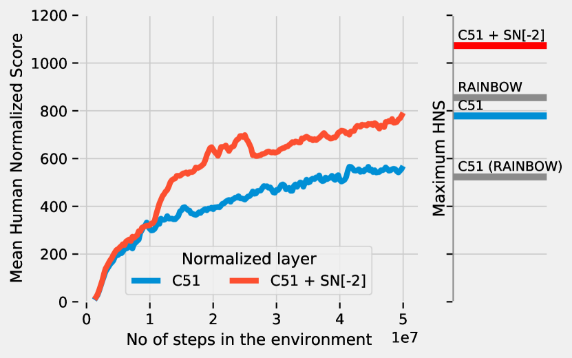
Figure 1: Optimisation rivals algorithmic improvements.
Left: Average Human Normalised Score (HNS) per time-step for C51 with Spectral Normalisation (SN). Right: Comparison of Maximum HNS reported in the literature (same as in Table 1). Average over 54 Arcade Learning Environment (ALE) games.

In our paper we explore Spectral Normalisation (SN), one such technique originating in the Generative Adversarial Networks (GANs) literature (Miyato et al., 2018), another field having to deal with non-stationarity and challenging optimisation dynamics. SN was primarily used for its regularisation effect of controlling the smoothness of the function. In (Farnia et al., 2018) authors rely on SN as a defense against adversarial examples, (Anil et al., 2019) for improving estimation of Wasserstein distance and (Yu et al., 2020) to regularise model-based Reinforcement Learning (RL).

However SN also decouples the norm of the weight vector from its direction, therefore affecting optimisation in subtle ways, especially in the case of adaptive, momentum based methods (Rosca et al., 2020).

Our main contributions in this paper are:

Efficiency of SN in DRL. We show that SN can lead to performance gains that rivals other algorithmic improvements such as those collated in the Rainbow agent (Fig. 1). We additionally provide code to ensure reproducibility.

Optimisation effect of SN. We investigate the role of SN and argue that its effect is primarily an optimisation one. Although we identify a small correlation between smoothness and performance in our careful ablation studies, we argue the effect of smoothness is secondary. In particular, we can mimic the impact of SN on the parameter updates without changing the function represented by the neural network, hence without smoothness constraints, recovering the performance of SN.

Reducing hyper-parameter sensitivity. We show through large scale experiments that SN can extend Adam’s range of usable hyper-parameters.

2 Background

2.1 Value based deep reinforcement learning

An RL problem is usually described as a Markov Decision Process (MDP) $\mathcal{M}=(\mathcal{S},{\cal A},P,r,{\rho_{0}},\gamma)$ consisting of state space $\mathcal{S}$, the set of all possible actions ${\cal A}$, a transition distribution $P(s^{\prime}|s,a)$ and a reward function $r:{\cal S}\times{\cal A}\rightarrow\mathbb{R}$. The goal of an agent is to find a policy $\pi$ that maximises the expected sum of discounted rewards: $Q^{\pi}(s,a)=\mathbb{E}_{s_{0}\sim{\rho_{0}},a_{t}~{}\sim\pi\left(s_{t}\right)}\left[\sum_{t=0}\gamma^{t}r(s_{t},a_{t})\right]$. An important class of algorithms rely on state-action values to find $\pi$. These approaches focus on minimising the temporal difference (TD) error to learn the $Q$-function and define $\pi$ greedily with respect to it. We are particularly interested in scenarios where $Q$ is approximated by a neural network. The prototypical algorithm is DQN (Mnih et al., 2015), where $Q$ is learned by minimising:

$${\cal L}(\theta)=\underset{\scriptsize(s,a,r,s^{\prime})\sim{\cal D}}{\mathbb{E}}\Big{(}Q_{\theta}(s,a)-\big{(}r+\gamma\max_{a^{\prime}}Q_{\theta^{\prime}}(s^{\prime},a^{\prime})\big{)}\Big{)}^{2}$$ (1)

In TD error (Eq. 1), the bootstrapped term uses held-back parameters $\theta^{\prime}$ to bring extra stability. During training random batches of transitions are sampled from the last million experiences which are kept in a replay buffer $\mathcal{D}$. This mitigates, but does not enforce the i.i.d. and stationarity assumption required by stochastic gradient descent.

Since DQN first reported human-level results on the ALE Atari environment, several refinements of the algorithm were proposed. A remarkable line of research proposes to model the distribution of the state-action value rather than just its mean. For example, C51 (Bellemare et al., 2017) predicts a categorical distribution of expected returns. Rainbow (Hessel et al., 2018) integrates several advances on top of C51: prioritised experience replay for improved data sampling (Schaul et al., 2016), n-step returns for lower variance bootstrap targets, double Q-learning for unbiasing estimates (Van Hasselt et al., 2016), disambiguation of state-action value estimates (Wang et al., 2016) and noisy nets for improved exploration (Fortunato et al., 2018).

An often overlooked aspect is that the emergence of RMSProp (Tieleman & Hinton, 2012) and Adam (Kingma & Ba, 2014) adaptive optimisation algorithms is closely linked with the recent success of DRL.

2.2 Spectral Normalisation

Spectral Normalisation (SN) is an approach for controlling the Lipschitz constant of certain families of parametric functions such as linear operators. While it can be defined more generally, for our purpose we will consider a function to be Lipschitz continuous in the $\ell_{2}$ norm if $\lVert f(\bm{x}_{1})-f(\bm{x}_{2})\rVert_{2}\leq k\lVert\bm{x}_{1}-\bm{x}_{2}\rVert_{2}$ and we call $k$ the Lipschitz constant of the function. A linear map $\bm{y}=\mathbf{W}\bm{x}$ is 1-Lipschitz ($k=1$) if $\lVert\mathbf{W}\bm{x}\rVert_{2}\leq\lVert\bm{x}\rVert_{2}$ for any $\bm{x}$. This makes it apparent that normalising the spectral radius (largest singular value) of $\mathbf{W}$ enforces the 1-Lipschitz constraint on the linear map $\mathbf{\hat{W}}=\mathbf{W}/\left\lVert\mathbf{W}\right\rVert_{2}=\rho^{-1}\mathbf{W}$. This holds for convolutions as they are linear operators. A function is $k$-Lipschitz if the largest singular value of $\lVert\mathbf{J}_{\mathbf{xy}}\rVert$ is bounded by $k$. We make use of this relation to characterise the local smoothness of the learned neural networks in Sec. 5.2.

The Lipschitz constant of a composition of two functions, $f_{1}$ with Lipschitz constant $k_{1}$ and $f_{2}$ with constant $k_{2}$, will be bounded by the product $k_{1}\cdot k_{2}$. This implies that the Lipschitz constant of a neural network can be bounded by setting the Lipschitz constant of each layer. For a complete overview over the Lipschitz constant of various layers, pooling and common activation functions including ReLU we refer to (Anil et al., 2019; Gouk et al., 2020).

3 Methods

Computing the spectral radius at each training step would be prohibitive, therefore we approximate it with one step of power iteration (Golub & van der Vorst, 2000) at every forward pass. The algorithm is sketched below with $\mathbf{u}$ and $\mathbf{v}$ being the right, and left singural vectors.

$$\mathbf{v} \leftarrow\mathbf{W}\mathbf{u}^{(t-1)}; \alpha \leftarrow\lVert\mathbf{v}\rVert; \mathbf{v}^{(t)} \leftarrow\alpha^{-1}\mathbf{v}$$

$$\mathbf{u} \leftarrow\mathbf{W}^{\intercal}\mathbf{v}^{(t)}; \rho \leftarrow\lVert\mathbf{u}\rVert; \mathbf{u}^{(t)} \leftarrow\rho^{-1}\mathbf{u}$$

We then use the spectral radius estimation to perform a hard projection of the parameters: $\mathbf{\hat{W}}=\mathbf{W}/\max(\lambda,\;\rho)$. In all our experiments $\lambda=1$ if not specified otherwise. For convolutional layers we adapt the procedure in (Gouk et al., 2020) and the two matrix-vector multiplications are replaced by convolutional and transposed convolutional operations.

3.1 Relaxations of Spectral Normalisation

Our first experiments with SN quickly highlighted several interesting observations. First, constraining all layers has a negative impact on the agent’s performance. This is not surprising, a priori there is no reason for the true $Q$-functions to be smooth. Actions can often lead to drastic changes in the score, where taking a single action at time $t$ forfeits the game while the same action at previous step might carry no significance, as for example in Pong when the paddle is close to the ball or in MS-PacMan when a ghost is close to the agent. This require very different values for close-by states, making the optimal $Q$ function non-smooth.

These initial findings made it apparent that controlling the amount of regularisation is required. To address similar issues, (Gouk et al., 2020) proposes changing the projection rule to $\mathbf{\hat{W}}_{i}=\mathbf{W}_{i}/\max(\lambda_{i},\lVert\mathbf{W}_{i}\rVert_{2})$ and conduct a hyper-parameter search for the layer specific constants $\lambda_{i}$.

In contrast, we apply the normalisation only on a few layers of the network. We found it best to apply normalisation to the layers with the largest number of weights (Figs. 2, 4). For value functions networks in DRL, such as the classic Deep Q-Networks (DQN) architecture, this tends to be the layer before the output layer. We further motivate and discuss our design decisions in Sec. 5.3.

Because of the bias towards normalising layers deeper in the network we will refer to the index of the layer being normalised in a notation akin to Python list indexing syntax. For layers of any depth SN[-1] will refer to the output layer and SN[-2] to the one before it, while SN[-2,-3] refers to both layers being normalised together.

4 Spectral Normalisation on the Atari suite

Our intuition is that SN plays a dual role: one of smoothing the function and one of altering the optimisation dynamics of the neural network. This dual role has already been hinted to in other settings with non-stationary effects, such as GANs (Rosca et al., 2020). DRL is also characterised by problematic data shifts during training, therefore we seek to find out whether SN has a positive effect for RL-agents as well, and isolate its effect to SN’s ability to either smooth the function or to affect the optimisation process.

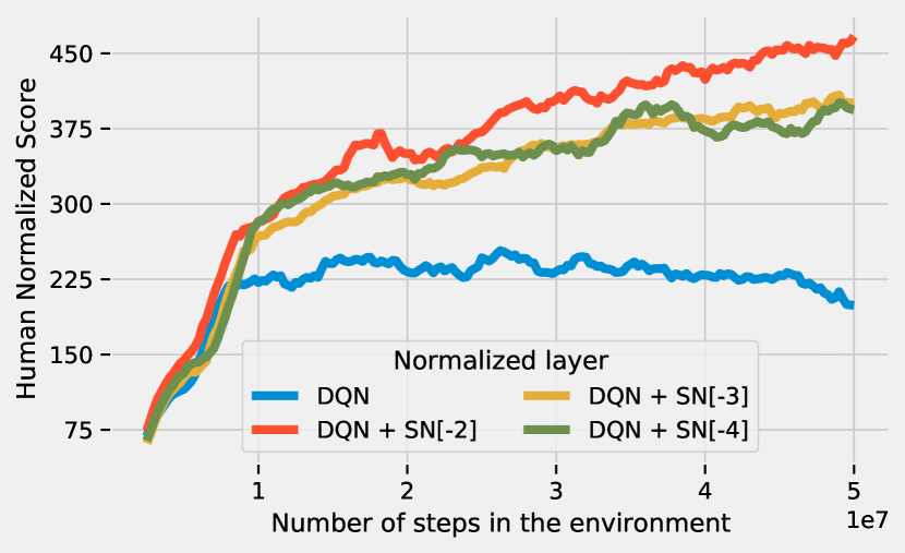
Figure 2: Human Normalised Score for a DQN-Adam baseline with SN applied on three different layers. Average over 54 Atari games.

To this end, we evaluate SN on the Arcade Learning Environment (ALE) (Bellemare et al., 2013). This collection of Atari games is varied and complex enough to ensure the generality of our claims and observations. Normalising only the penultimate layer (SN[-2]) while keeping everything else fixed enhances the performance of Categorical DQN (C51) beyond that of Rainbow(Fig. 1, Table 1) an agent that aggregates the advantages of many other RL advances on top of C51.

Agent	Mean	Median
DQN (Wang et al., 2016)	216.84	78.37
DQN-Adam∗	358.45	119.45
DQN-Adam SN[-2]	719.95	178.18
C51 (Hessel et al., 2018)	523.06	146.73
C51 (Bellemare et al., 2017)	633.49	174.84
C51∗	778.68	182.26
Rainbow (Hessel et al., 2018)	855.11	227.05
C51 SN[-2]	1073.18	248.45

Table 1: Mean and median Human Normalised Score on 54 Atari games with random starts evaluation. References indicate the sources for the scores for each algorithm. We mark our own implementations of the baseline with $\ast$. Our agents are evaluated with the protocol in (Hessel et al., 2018).

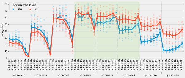
(a)

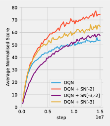
(b)

Figure 3: Left: SN decreases hyper-parameter sensitivity in Adam. Each $\{\eta,\epsilon\}$ combination is used to train 6 models of different depth and width on four MinAtar games, two seeds each. Dots represent the average maximum normalised score over the four games. Right: SN networks are more adaptable. On a $15$M steps training run the normalised agents continue to learn, adapting to increasingly difficult dynamics while the baseline plateaus. Each line is an average of 10 seeds over four MinAtar games and four different model sizes.

SN also demonstrates strong performance in the case of non-distributional value-based methods. Results on smaller environments suggested that SN is less effective in conjunction with RMSProp therefore we train a DQN agent using the Adam optimiser instead of RMSProp. We use the optimiser settings and other hyper-parameters found in Dopamine (Castro et al., 2018) as detailed in appendix C.2. We keep the rest of the training and evaluation protocol similar to that of the other algorithms we compare with. Note that with this change we are not weakening the baseline. We show that applying SN to any of the hidden layers significantly improves upon the DQN baseline (Fig. 2). Moreover, the performance closes in on our own implementation of C51 further suggesting that performance gains coming from optimisation and regularisation advances may be comparable to those achieved by RL-centric methods. We consolidate all these results in Table 1 on a subset of 54 games . We note that we did not fine-tune our normalised variants but rather reused the same hyper-parameters as for the baseline. These hyper-parameters are the result of careful tuning reported in the literature and are detailed in appendix C. We also report results for DQN trained with RMSprop in Sec. C.3.

The mean and median Human Normalised Score have been critiqued in the past (Machado et al., 2018; Toromanoff et al., 2019) because they can be dominated by some large normalised scores. However we notice that with very few exceptions ($3/54$ for DQN and $11/54$ games for C51, Fig. C) normalising at most one of the network’s layers will not degrade the performance compared to the baseline but instead it will improve upon it, often substantially.

5 Analysis of results

In order to understand the strong performance of SN in Atari we proceed to answer several questions employing both large-scale experiments and technical arguments: How is SN interfering with optimisation? Is smoothness a factor in the performance we are observing? And are other regularisation methods leading to similar empirical gains?

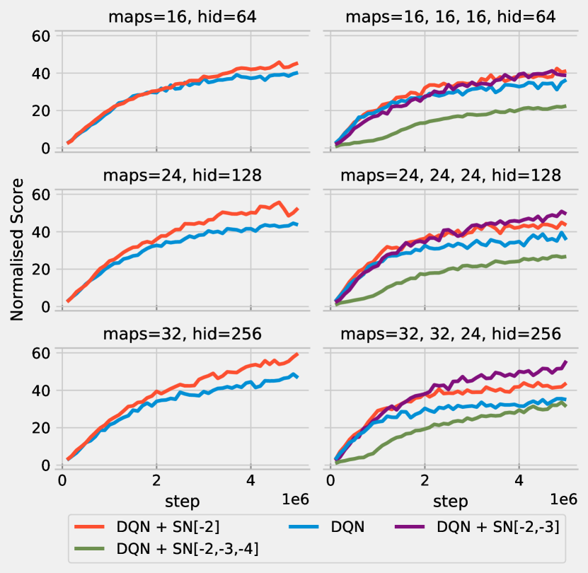
Figure 4: SN shows gains for all model sizes. We note two regimes of the DQN baseline ( ): for shallow models performance increases with the width of the model; for deeper models performance stagnates with increasing depth and width. In both regimes applying SN on individual ( ) or multiple ( ) layers improves on DQN suggesting a regularisation effect we could not reproduce with other methods (Fig. 16). Normalising too many layers ( ) decreases the capacity and is detrimental to learning. Normalised scores of 4 games $\times$ 10 seeds. Details in Fig. 12.

Since the large scale study we require would have been prohibitive in ALE, all the experiments in this section if not mentioned otherwise are using for evaluation the MinAtar environment (Young & Tian, 2019) which reproduces five games from ALE complete with their non-stationary dynamics but without the visual complexity. MinAtar was found to be well-suited for reproducing the ablations of recent DRL contributions originally made on ALE (Obando-Ceron & Castro, 2020) and therefore we adopt it for our purposes.

Most of the MinAtar results we report are averages of normalised scores over four games. All agents employ an architecture with at least one convolutional layer and two final linear layers. When varying the depth of the architecture we only adjust the number of convolutional layers. When varying the width we increase the number of both feature maps and units in the linear layers.

5.1 Spectral Normalisation decreases hyper-parameter sensitivity

We characterise empirically the impact SN has on an agent’s performance with a wide variety of architectures and optimisation settings. In particular, we consider six models of different depths and widths, many learning rates and epsilon values for both Adam and RMSProp with and without SN or layer [-2] or layers [-2,-3] for four different games, two seeds for each configuration, resulting in $14000$ DQN agents. Fig. 3 reveals several interesting observations:

1. SN almost never degrades the performance of the baseline therefore it can be safely used in existing agents.

2. SN extends the usable range of Adam’s hyper-parameters. Assuming ideal hyper-parameters for the un-normalised network, which typically reside in a very narrow hyper-parameter subspace, applying SN does not harm performance. However the normalised model performs well within a significantly larger range, highlighted by the green band in Fig. 3, while the baseline degrades dramatically.

3. SN allows for increased adaptability to changing dynamics in the environment. MinAtar share with ALE the property of increasing in difficulty as the policy improves. On a 15M training run (Fig. 3, right) SN demonstrates it can continue to learn better policies while the baseline plateaus. This finding is also supported on Atari (Fig. 2).

5.2 Smoothness and performance are weakly correlated

The Lipschitz constant of a neural network can be at most the product of the Lipschitz constants of its layers. Since in this work we normalise only a subset of layers, we naturally ask whether it is enough to produce smoother functions. Also, we seek to answer whether performance correlates with the smoothness of the function.

While the exact computation of $k$ for a network is NP-hard (Virmaux & Scaman, 2018) we can compute a local smoothness measure with respect to the data distribution. To approximate the smoothness of our learned value functions we trained agents equipped with twelve different model sizes. For each game-architecture combination we trained a DQN baseline and normalised various layers, 10 seeds each, resulting in 2400 trained agents. We then used the best checkpoint for each combination to sample 100k steps in the game and compute for each state $\mathbf{s}$ the norm of the gradient of the state-action value with respect to the state and we report the largest norm encountered.

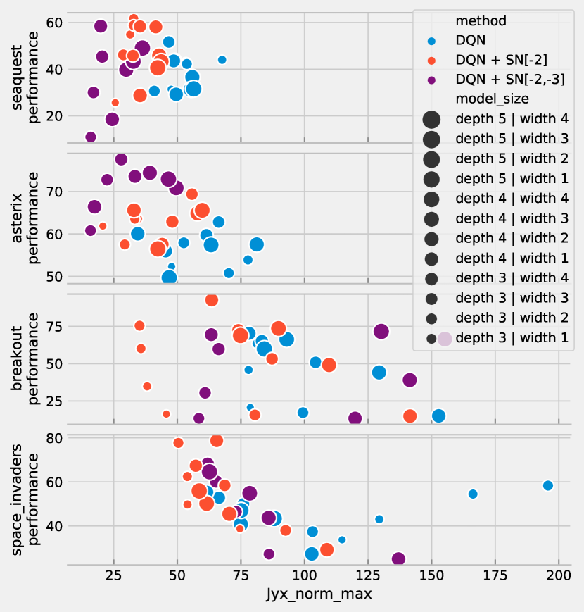
Figure 5: SN does not consistently produce smoother networks. Often normalising a subset of the network’s layers makes the network less smooth than the baseline while performance improves still. MinAtar games, average over 10 seeds, for completeness refer to Fig. 14

We note that while a slight correlation can be measured using Spearman’s rank, SN does not generally produce smoother networks. The relation between performance and smoothness is not consistent across MDPs, ranging from strong dependence in Space Invaders to no correlation in Breakout (see Fig. 5). The baseline of a three-layer network exhibits a higher empirical norm of the Jacobian than any of the normalised models but this is not the case for deeper models. For models larger than three layers the top-performing normalised experiments exhibit a smoothness similar to that of the baseline but also increased performance. A detailed description of the setup and results can be found in appendix B.3. In conclusion, smoothness does not fully account for the higher performance brought by SN.

To further explore a possible connection between smoothness and performance we did several experiments with other regularisation methods. First we perform a careful tuning of Gradient Penalty (GP) (Gulrajani et al., 2017) as an alternative method of imposing smoothness constraints on the learned action-value functions and we found it generally hurts performance and at best it makes no difference. We then considered Batch Normalisation (BN) (Ioffe & Szegedy, 2015) for its ability to control the Lipschitz constant of the loss function w.r.t. the parameters (Santurkar et al., 2018), but also generally thought to improve the optimisation properties of neural networks (Arora et al., 2018). We once again found it degrades performance, which is also consistent with the DRL literature in the small batch-size regime (Bhatt et al., 2019). We give the full details in supplementary B.4.

5.3 Limitations of 1-Lipschitz networks and practical considerations

Fig. 4 characterises the performance of SN as a function of the model size and the number of normalised layers. SN generally leads to a good performance when a small number of layers are targeted. However, normalising more than half of the number of layers in a depth-5 network results in degraded behaviour suggesting a too strong regularisation effect (see Appendix Fig. 12).

We find this to be consistent with prior work showing that when ReLU networks are constrained to be 1-Lipschitz by applying SN to all their layers, it reduces the range of functions they can express (Huster et al., 2018; Anil et al., 2019). Related, smoothness regularisation methods are generally employed with small coefficients in order to avoid performance penalties. For example Spectral Norm Regularisation (SR) in (Yoshida & Miyato, 2017) uses a coefficient $\lambda=0.01$ and the orthogonality regularisation in Parseval Networks (Cissé et al., 2017) uses a $\beta\in\{0.0001,0.0003\}$ which can make the network to be far from 1-Lipschitz as discussed in (Anil et al., 2019). When SN is deployed in the adversarial robustness task (Gouk et al., 2020), the optimal $\lambda_{i}$ values for different layer types were found in the range $\{2,..,50\}$, a considerable departure from the 1-Lipschitz bound for the entire network. We find these reports of relaxing the 1-Lipschitz constraint consistent with our selective SN design choice.

5.4 Spectral Normalisation has primarily an optimisation effect

We claim that SN improves the performance of the value-function estimator by affecting the optimisation dynamics. Precisely, SN provides a scheduler that adapts the size and the direction of the optimisation step as the weights increase during training. In the case of Adam (Kingma & Ba, 2014) SN could be compensating for how curvature is being approximated in the late training regime by the expected squared gradient which should vanish at convergence.

We start by comparing the gradients of the normalised neural network with those of its standard counterpart. We then build two incremental approximations to SN which directly affect the optimisation step using the spectral radius. We provide empirical evidence that these data-dependent alterations of the optimiser recover and sometimes surpass the performance boost from SN, supporting our optimisation interpretation of the method.

Consider a feed-forward estimator with $L$ parametric layers (for brevity we will assume linear projections, although everything applies to convolutions as well). All except the last layer are followed by rectifiers.

$$\mathbf{a}_{0} \triangleq\mathbf{x}$$ (2)

$$\mathbf{z}_{i} =\mathbf{W}_{i}\mathbf{a}_{i-1}+\mathbf{b}_{i} 1\leq i\leq L$$ (3)

$$\mathbf{a}_{i} =\operatorname{ReLU}\left(\mathbf{z}_{i}\right) 1\leq i<L$$ (4)

We impose that a subset of layers $\mathcal{S}\subseteq\left\{1,2,\ldots,L\right\}$ are individually $k$-Lipschitz continuous by using normalised parameters $\forall i\in\mathcal{S}:\mathbf{\hat{W}}_{i}=\rho_{i}^{-1}\mathbf{W}_{i}$ with $\rho_{i}=\max\left(\langle\rho\left(\mathbf{W}_{i}\right)\rangle,k\right)$. We use $\rho\left(\cdot\right)$ to denote the spectral radius (i.e. the largest singular value of $\mathbf{W}_{i}$) and $\langle\cdot\rangle$ for the stop gradient function, using hat notations for all the quantities in the normalised network: $\mathbf{\hat{z}}_{i}=\mathbf{\hat{W}}_{i}\mathbf{\hat{a}}_{i-1}+\mathbf{b}_{i}$. Since the bias is not scaled along with the weights, the sign of the pre-activations is not preserved ($\left[\mathbf{z}_{i}>0\right]\neq\left[\mathbf{\hat{z}}_{i}>0\right]$) therefore one cannot write an explicit relation between $\frac{\partial{\mathcal{L}}}{\partial{\mathbf{W}_{i}}}$ and $\frac{\partial{\hat{\mathcal{L}}}}{\partial{\mathbf{W}_{i}}}$. We will now make a slight modification to SN such that writing such a relation becomes possible.

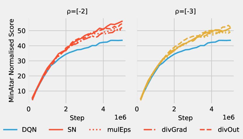
Figure 6: Spectral schedulers recover SN performance. Average normalised scores over MinAtar games and four different models. Refer to Fig.18 for completion.

Bias scaling.

Consider the following alteration of the spectral normalisation procedure presented above. As before, we perform spectral normalisation on a subset of layers $\mathcal{S}$. In addition, for each normalised layer $l\in\mathcal{S}$ we also scale the bias terms of subsequent layers $i>l$ with $\rho_{l}^{-1}$ as shown in Eq. 7. By doing so we can relate the pre-activations $\mathbf{\hat{z}}_{i}$ on all layers to those from the unnormalised Multi-Layer Perceptron (MLP) described in Eq. 3:

$$\rho^{-1}_{i:j} \triangleq\prod_{i\leq k\leq j\wedge k\in\mathcal{S}}\rho^{-1}_{k}$$ (5)

$$\mathbf{\hat{z}}_{i} =\rho_{i}^{-1}\left(\mathbf{W}_{i}\mathbf{\hat{a}}_{i-1}+\rho^{-1}_{1:i-1}\mathbf{b}_{i}\right)$$ (6)

$$=\rho_{i}^{-1}\mathbf{W}_{i}\mathbf{\hat{a}}_{i-1}+\rho_{1:i}\mathbf{b}_{i}=\rho^{-1}_{1:i}\mathbf{z}_{i}$$ (7)

$$\hat{\mathcal{L}} \triangleq\operatorname{loss}\left(\mathbf{\hat{z}}_{L}\right)=\operatorname{loss}\left(\rho^{-1}_{1:i}\mathbf{z}_{i}\right)$$ (8)

We can now compute the gradients w.r.t. the unnormalised parameters for both the standard estimator and the normalised one with scaled biases:

SN+bias scaling

$$\frac{\partial{\mathcal{L}}}{\partial{\mathbf{W}_{i}}} =\mathbf{J}_{i}\boldsymbol{\delta}_{L}\mathbf{a}_{i-1}^{\intercal} \frac{\partial{\hat{\mathcal{L}}}}{\partial{\mathbf{W}_{i}}} =\rho^{-1}\mathbf{J}_{i}\boldsymbol{\hat{\delta}}_{L}\mathbf{a}_{i-1}^{\intercal}$$ (9)

$$\frac{\partial{\mathcal{L}}}{\partial{\mathbf{b}_{i}}} =\mathbf{J}_{i}\boldsymbol{\delta}_{L} \frac{\partial{\hat{\mathcal{L}}}}{\partial{\mathbf{b}_{i}}} =\rho^{-1}\mathbf{J}_{i}\boldsymbol{\hat{\delta}}_{L}$$ (10)

where $\rho^{-1}\triangleq\prod_{i\in\mathcal{S}}\rho_{i}^{-1}$; the jacobian w.r.t. estimator’s outputs: $\boldsymbol{\hat{\delta}}_{L}\triangleq\frac{\partial{\hat{\mathcal{L}}}}{\partial{\mathbf{\hat{z}}_{L}}}$; and $\mathbf{J}_{i}\triangleq\prod_{j=i}^{L-1}\left[\operatorname{diag}\left(\left[\mathbf{z}_{j}>0\right]\right)\mathbf{W}_{j+1}^{\intercal}\right]$.

Output scaling.

The right-hand expressions in Eq. 9 and 10 show that SN+bias scaling is computationally equivalent with simply scaling the un-normalised network’s output with $\rho^{-1}$. Doing so yields the same gradients as SN+bias scaling, reducing the importance of the depths where weights are conditioned. We refer to this approximations as divOut. We argue that outside some pathological cases, the bias terms easily adapt to the layer’s mean activation in both cases therefore SN and divOut should have similar behaviours. Indeed, experiments performed on MinAtar confirm that the divOut approximation recovers the performance of SN (see Figure 6). Inspecting the performance on multiple architectures and normalisations we also observe that divOut fails to learn when SN fails (Fig. 18 in Appendix). We therefore consider SN + bias scaling (and its equivalent formulation divOut) a reasonable proxy to study the effects of SN.

The gradient scaling effect.

Eq. 9, and 10 show that the effect SN+bias scaling has on the updates is two-fold. First, gradients are scaled by $\rho^{-1}$. Second, the model changes, therefore the jacobians of the loss function with respect to the network’s output changes: $\boldsymbol{\delta}_{L}\neq\boldsymbol{\hat{\delta}}_{L}$. We argue that specifically for DQN where the TD-error is put in a Huber cost, there is no evident scaling relation between $\boldsymbol{\delta}_{L}$ and $\boldsymbol{\hat{\delta}}_{L}$ (for values larger than 1, the gradient is just the sign of $y-t$). We therefore isolate the first effect, i.e. scaling the gradients with the inverse spectral radius before passing it to the gradient based optimiser, in a scheduler we name divGrad.

We again evaluate this scheduler using multiple architectures and sets of spectral radii on the games in MinAtar. The averaged learning curves in Figure 6 demonstrate that this gradient scaling effect of SN is sufficient to explain the performance gain, indicating that SN actually proposes better optimisation steps rather than conditioning the network in a better subspace.

We also notice that divGrad improves the performance of DQN event when the spectral norms of all hidden layers are considered, case in which SN fails to train (Figure 7).

Interactions with Adam.

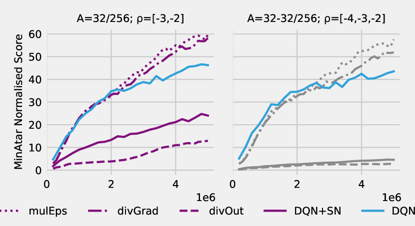
Figure 7: Spectral schedulers improve performance even when the radii of all layers are used. In these cases SN fails to train. Minatar Normalised Score for two models. Refer to Fig.18 for completion.

In order to account for the surprising performance of divGrad, we study its effect when the optimiser used is Adam (Kingma & Ba, 2014) (Eqs. 11, 12, 13), the recent first choice for optimising DRL algorithms. To do that we compare an optimisation step in a regular MLP with the same quantity when gradients are inversely scaled with the spectral radius.

$$\mathbf{v}_{t+1} \longleftarrow\beta_{1}\mathbf{v}_{t}+\left(1-\beta_{1}\right)\mathbf{g}_{t}$$ (11)

$$\mathbf{s}_{t+1} \longleftarrow\beta_{2}\mathbf{s}_{t}+\left(1-\beta_{2}\right)\mathbf{g}^{2}_{t}$$ (12)

$$\Delta\mathbf{W}_{t} \triangleq\eta\frac{\left(1-\beta_{1}^{t}\right)^{-1}\mathbf{v}_{t+1}}{\sqrt{\left(1-\beta_{2}^{t}\right)^{-1}\mathbf{s}_{t+1}}+\epsilon}$$ (13)

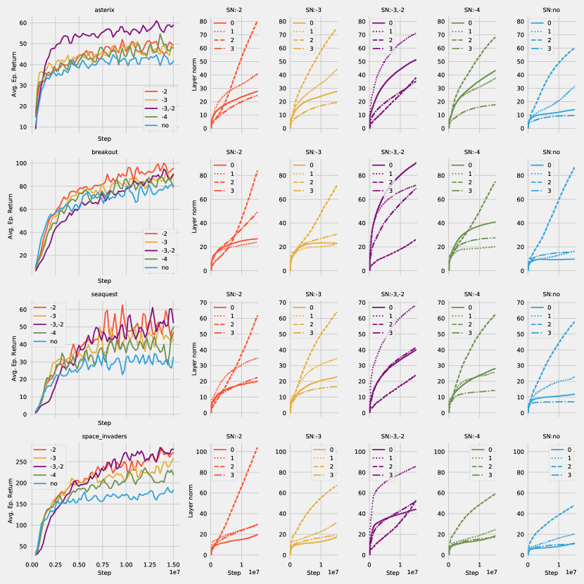
Figure 13: All spectral radii for the 15M experiment on MinAtar using a 4-layer architecture (conv=24-24,fc=128). Colors code the subsets of layers that are normalised (consistent with the rest of the document), while line styles code the four layers. Note how the penultimate layer has the largest spectral norm across all normalisation variants. 10 seeds.

The spectral radius changes slowly during training (Fig.13 in Appendix), making it reasonable to approximate the exponentially decayed sums in $\hat{\mathbf{v}}_{t}$, and $\hat{\mathbf{v}}_{t}$:

$$\mathbf{v}^{{}^{\prime}}_{t+1} \approx\rho_{t}^{-1}\mathbf{v}_{t+1}$$ (14)

$$\mathbf{s}^{{}^{\prime}}_{t+1} \approx\rho_{t}^{-2}\mathbf{s}_{t+1}$$ (15)

$$\Delta\mathbf{W}_{t}^{{}^{\prime}} \approx\eta\frac{\left(1-\beta_{1}^{t}\right)^{-1}\mathbf{v}_{t+1}}{\sqrt{\left(1-\beta_{2}^{t}\right)^{-1}\mathbf{s}_{t+1}}+\rho_{t}\epsilon}$$ (16)

It means that (in a instantaneous comparison with the gradient for the unregularized network) the step size when applying gradient scaling with a slowly increasing $\rho$ reduces the learning rate while making the projection closer and closer to SGD with momentum. Or, equivalently, as learning progresses the curvature approximation in the denominator is dominated by the uniform scale factor $\rho\epsilon$. We therefore propose a scheduler (mulEps) where we multiply the $\epsilon$ term by the product of spectral radii as in Eq. 16 , expecting a close behaviour to that of divGrad. Experiments on MinAtar confirm this, providing a possible interpretation for the efficiency of SN, namely that it modulates $\epsilon$.

While in Supervised Learning (SL) $\epsilon$ is mostly used for numerical stability, its role in dealing with unreliable approximation of the curvature has been considered. Since gradient statistics are typically assumed to be unreliable early in training (Liu et al., 2019), a decreasing schedule for the damping factor was suggested in (Martens & Grosse, 2015). However these heuristics do not seem to match the needs of DRL. This is emphasised by the typical use of much higher $\epsilon$ in DRL (Bellemare et al., 2017; Mnih et al., 2015) and by our findings, suggesting the modulation of $\epsilon$.

6 Related work

SN and its penalty term formulation Spectral Norm Regularisation (SR) (Yoshida & Miyato, 2017), have been mostly researched in the context of regularisation for example as a defense against adversarial examples (Tsuzuku et al., 2018; Farnia et al., 2018; Gouk et al., 2020), to improve the stability of Generative Adversarial Network (GAN) training (Kurach et al., 2019) or to improve robustness of uncertainty estimates (Liu et al., 2020). It was recently used in DRL (Yu et al., 2020) also in the context of robust uncertainty estimation for model based RL. However the optimisation effect investigated in Sec. 5 has not been considered. (Rosca et al., 2020) provides a thorough overview of the current understanding of smoothness constraints, applications and methods, including SN.

Probably the most related method that has been extensively studied from an optimisation perspective is Weight Normalisation (WN) (Salimans & Kingma, 2016). Similary to SN they rely on a hard projection $\mathbf{\hat{W}}_{i}=g\mathbf{v}/\lVert\mathbf{v}\rVert_{F}$, with the exception that $g$ is learned and the use of a simpler Frobenius matrix norm. The authors also report results on a subset of ALE environments for DQN, showing gains over the baseline. (Miyato et al., 2018) contrasts SN and WN and argue that the Frobenius norm encourages a loss in the number of usable features of the learned representations. Our experiments support this argument: measuring the effective rank (Kumar et al., 2020) shows a faster loss of feature rank for the baseline agent compared to any SN agent (Fig. 21 in Appendix). Since WN fuels a loss in rank we believe this might explain the performance difference between the two.

SN together with WN and Batch Normalisation (BN) (Ioffe & Szegedy, 2015), are part of a larger family of normalisation methods that make the layer invariant to change in the scale of the parameters. In (Van Laarhoven, 2017; Hoffer et al., 2018; Arora et al., 2018) the authors study the effect of L2 regularisation in BN and WN networks deriving an effective learning rate $\eta^{\prime}=\eta/\lVert\mathbf{W}\rVert$ that depends on the evolution of the weight norm. They also show that the norm interacts with the damping factor in adaptive algorithms, including Adam, such that $\epsilon^{\prime}=\epsilon\lVert\mathbf{W}\rVert$ effectively behaving as a scheduler on these hyper-parameters. Our analysis in Sec. 5.4 looks at the relation between the regular and normalised update steps and identifies a similar scaling factor of the damping term, while preserving the learning rate.

The damping term $\epsilon$ has been often overlooked in SL and relegated only to numerical stability, however in DRL it is usually set rather high in both Adam and RMSprop without a justification. We believe part of the gains we report is due to the implicit scheduling of $\epsilon$. We corroborate this finding with work on accurate approximation of the curvature of the loss function where scheduling the Tikhonov damping is proposed. For example, in K-FAC, the damping value starts high and it is decreased as the information about curvature improves (Martens, 2010; Martens & Grosse, 2015). The $\epsilon$ term in Adam has a similar purpose but on a weaker approximation of the curvature based on the Empirical Fisher Information Matrix (Pascanu & Bengio, 2014; Kunstner et al., 2019). Our study in Sec. 5.4 suggests that in DRL this approximation is even more deficient and does not improve during training, as in general we see a benefit from the monotonic increase of the damping factor.

Recent works address the optimisation issues specific to TD learning. (Bengio et al., 2020) discusses the negative interplay between the adaptive methods from SL (RMSprop, Adam) and TD(0). Others propose optimisers for RL, but they are either restricted to linear estimators (Givchi & Palhang, 2014; Sun et al., 2020), or they show no empirical advantages (Romoff et al., 2020).

7 Conclusion

We identify and characterise the strong performance boost when applying Spectral Normalisation (SN) on the network DRL agents use for state-action value estimation. Through careful ablations on a large number of architectures and settings we disentangle between smoothness and optimisation effects. We find that rather than restricting the irregularities of the network function, SN changes the optimisation dynamics providing a good scheduler. We also derive explicit schedulers by moving the spectral norm in the update step of Adam and show that these recover the performance of SN. These observations suggest there is much to gain by designing better adapting optimisers for DRL.

Appendix A Methods

A.1 Computing the spectral norm

Power Iteration.

Computing the dominant singular value at each step would be expensive, therefore spectral normalisation is usually performed through power iteration. For each set of weights $\mathbf{W}_{i}\in\mathbb{R}^{N_{i}\times N_{i-1}}:i\in\mathcal{S}$ the corresponding left and right singular vectors are stored, and two extra matrix-vector multiplications for each normalised layer are performed at each forward pass (see Formulas 17, 18). At inference time there is no extra computational cost.

$$\mathbf{v} \leftarrow\mathbf{W}_{i}\mathbf{u}^{(t-1)}; \alpha \leftarrow\lVert\mathbf{v}\rVert; \mathbf{v}^{(t)} \leftarrow\alpha^{-1}\mathbf{v}$$ (17)

$$\mathbf{u} \leftarrow\mathbf{W}_{i}^{\intercal}\mathbf{v}^{(t)}; \rho \leftarrow\lVert\mathbf{u}\rVert; \mathbf{u}^{(t)} \leftarrow\rho^{-1}\mathbf{u}$$ (18)

For convolutional layers we adapt the procedure in (Gouk et al., 2020) and the two matrix-vector multiplications are replaced by convolutional and transposed convolutional operations.

Backpropagating through the norm.

Since the parameters that are tuned during optimisation are the unnormalised weights $\mathbf{W}_{i}$, we investigated if there are any advantages in backpropagating through the power iteration step, i.e. considering the partial derivative $\frac{\partial\mathbf{\hat{W}}_{i}}{\partial\rho_{i}}\frac{\partial\rho_{i}}{\partial\mathbf{W}_{i}}$ when computing the gradient. Precisely, we verified if dropping the second term in the right-hand side of Formula 19 biases the gradient.

$$\frac{\partial\mathcal{L}}{\partial\mathbf{W}_{i}}=\rho_{i}^{-1}\frac{\partial\mathcal{L}}{\partial\mathbf{\hat{W}}_{i}}-\rho_{i}^{-2}\mathbf{u}\mathbf{v}^{\intercal}\left(vec\left(\frac{\partial\mathcal{L}}{\partial\mathbf{\hat{W}}_{i}}\right)vec\left(\mathbf{W}_{i}\right)\right)$$ (19)

In a batch of experiments performed on a subset of games of Atari we noticed no loss in performance when dropping the Jacobian from the power iteration.

A.2 Computing the norm of the Jacobians

Experiments in Sec. 5.2 used the maximum norm of the jacobians w.r.t. the inputs as an indirect metric for network function’s smoothness. For each network we collected thousands of states (on-policy), computing the maximum euclidean norm of the jacobian w.r.t. the inputs: $\max_{i,\mathbf{x}}||\frac{\partial q_{i}\left(\mathbf{x};\theta\right)}{\partial\mathbf{x}}||_{2}$. Note that we used the euclidean norm (and not the operator norm) to measure smoothness.

Appendix B MinAtar experiments

Game selection.

MinAtar (Young & Tian, 2019) benchmark is a collection of five games that reproduce the dynamics of Arcade Learning Environment (ALE) counterparts, albeit in a smaller observational space. Out of Asterix, Breakout, Seaquest, Space Invaders and Freeway we excluded the latter from all our experiments since all the agents performed essentially the same on this game.

Network architecture.

All experiments on MinAtar are using a convolutional network with $L_{C}$ convolutional layers with the same number of channels, a hidden linear layer, and the output layer. The number of input channels is game-dependent in MinAtar. All convolutional layers have a kernel size of $3$ and a stride of $1$. All hidden layers have rectified linear units. Whenever we vary depth we change the number of convolutional layers $L_{C}$, keeping the two linear layers. When the width is varied we change the width of both convolutional layers (e.g. 16/24/32 channels) and the penultimate linear layer. All convolutional layers are always identically scaled.

We list all the architectures used in various experiments described in this section in Table 6.

General hyper-parameter settings.

In all our MinAtar experiments we used the same set of hyper-parameters returned by a small grid search around the initial values published by (Young & Tian, 2019). We list the values we settled on in Table 2. For the rest of this section we only mention how we deviate from this set of hyper-parameters and settings for each of the experiments that follow.

Hyper-parameter	Value
discount $\gamma$	0.99
update frequency	4
target update frequency	4,000
starting $\epsilon$	1.0
final $\epsilon$	0.01
$\epsilon$ steps	250,000
$\epsilon$ schedule	linear
warmup steps	5,000
replay size	100,000
history length	1
cost function	MSE Loss
optimiser	Adam
learning rate $\eta$	0.00025
damping term $\epsilon$	0.0003125
$\beta_{1},\beta_{2}$	(0.9, 0.999)
validation steps	125000
validation $\epsilon$	0.001

Table 2: MinAtar general hyper-parameter settings.

MinAtar Normalised Score.

In our work we present many MinAtar experiments as averages over the four games we tested on. Since in MinAtar the range of the expected returns is game dependent we normalise the score. Inspired by the Human Normalised Score in (Mnih et al., 2015) we take the largest score ever recorded by a baseline agent in our experiments and use it to compute $\text{MNS}=100\times(\text{score}_{\text{agent}}-\text{score}_{\text{random}})/(\text{score}_{\text{max}}-\text{score}_{\text{random}})$. We can then use the resulting MinAtar Normalised Score whenever we need to report performance aggregates over the games.

Game	Max	Random
Asterix	78.90	0.49
Breakout	122.88	0.52
Seaquest	93.91	0.09
Space Invaders	360.92	2.86

Table 3: MinAtar maximum and random scores used for computing the MinAtar Normalised Score.

B.1 Large optimiser hyper-parameter sweep

For the large optimiser hyper-parameter sweep we train a DQN agent with six different architectures as listed in Table 6. For each architecture we then trained on all combinations of optimisation hyper-parameters (from the lists below), both normalised and baseline agents, two seeds each. We generated values for the learning rate using a geometric progression in the following ranges:

Optimiser	Hyper-parameters
Adam	$\eta$: $\{0.00001,...,0.00215\}$ $\epsilon$: $\{0.00001,...,0.01\}$
RMSprop	$\eta$: $\{0.00001,...,0.001\}$ $\epsilon$: $\{0.00001,...,0.0316\}$ $\alpha\in\{0.95\}$ centered: yes
Adam	$\eta$: $\{0.00001,...,0.001\}$

Table 4: Hyper-parameters ranges for the large optimiser sweep.

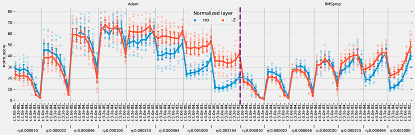
Figure 8: Spectral Normalisation increases the range of effective optimisation settings. Each configuration is used to train 6 models of different depth and width on four MinAtar games, two seeds each. Dots represent the average maximum normalised score over the four games.

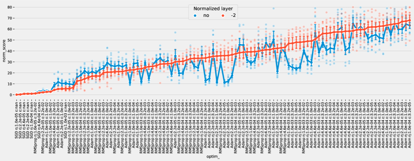
Figure 9: Spectral Normalisation improves on the baseline on a wide range of optimisation settings. Each optimisation setting is used to train 6 models of different depths and widths on four MinAtar games, two seeds each. Dots represent the average MinAtar Normalised Score achieved over four games. We sort by the mean performance of the SN experiment and show the baseline stays mostly under this curve in the region of high performance optimiser configurations.

Figure 8 illustrates our findings. In the case of Adam optimiser we can see that normalising one layer does not degrade the performance of the baseline and allows for larger learning rates. A similar observation can be made for RMSprop and exploring learning rates larges than $0.001$ should clarify to what degree the trend already visibile continues.

Figure 9 is a different visualisation of the same results. Here we sort the x-axis by the mean normalised score of an optimiser configuration for the DQN agents equipped with SN and plot both the performance of the baseline and the normalised experiments. We show that the performance of the normalised agent generally outperforms the baseline, especially in the right half of the plot corresponding with higher performance agents.

B.2 Effect on model capacity

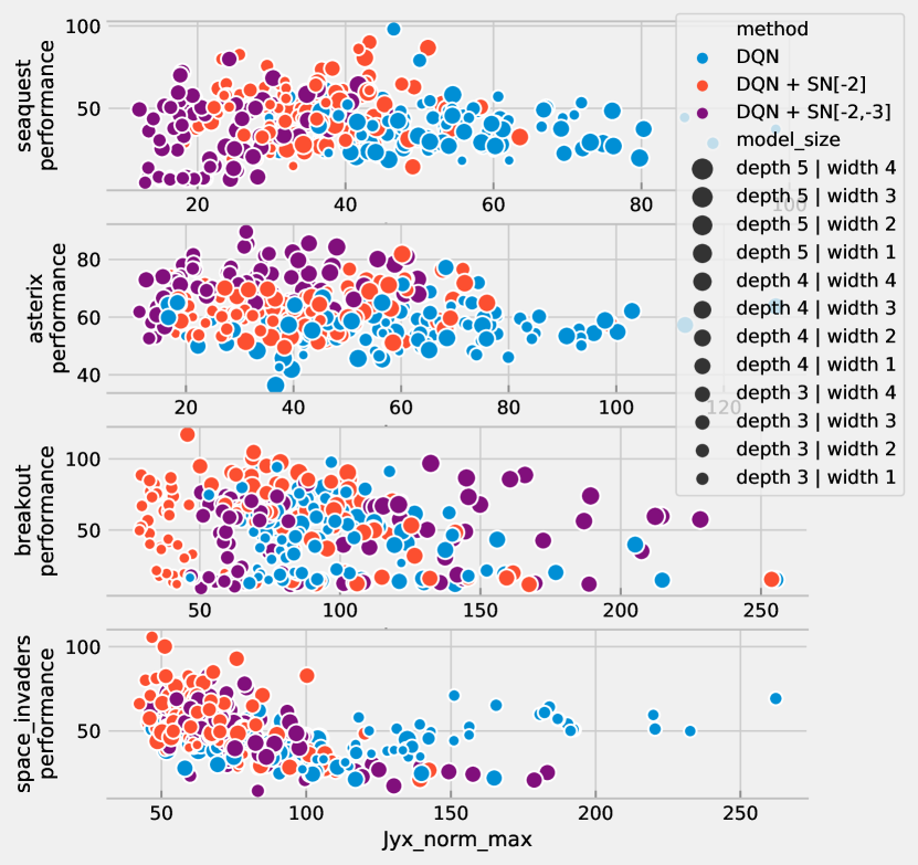
Figure 14: Applying SN on a layer subset does not consistently produce smoother networks. Often normalising a subset of the network’s layers makes the network less smooth than the baseline while performance improves still. Each point in the graph represents the maximum performance achieved by a single seed. Detailed view of Fig. 5

.

For understanding the effect of SN on model capacity we train DQN agents with 12 different model sizes of three different depths and four different widths. We apply SN on various layer subsets and report in Figure 12 the MinAtar Normalised Score averaged over the four games. All the other parameters remain the same as described at the beginning of this section. Each resulting game-architecture combination was trained on $10$ seeds.

B.3 Smoothness and performance are weakly correlated

In Figure 14 we plot the peak performance and the norm of the Jacobian for each of the seeds in the experiment we discuss in Section B.3 instead of averages.

Computing a correlation measure for all the normalisation schemes in the experiment is complicated by the fact that any selection we make affects the correlation we want to measure. Limiting ourselves to just the baseline and DQN[-2], the normalisation scheme we have shown repeatedly that it does not hurt performance, we computed the Spearman rank-order correlation we report in Table 5.

Game	Spearman Rank
Asterix	-0.129
Breakout	-0.199
Seaquest	-0.151
Space Invaders	-0.453

Table 5: Correlation between the norm of the Jacobian and peak performance for each game.

B.4 Other regularisation methods

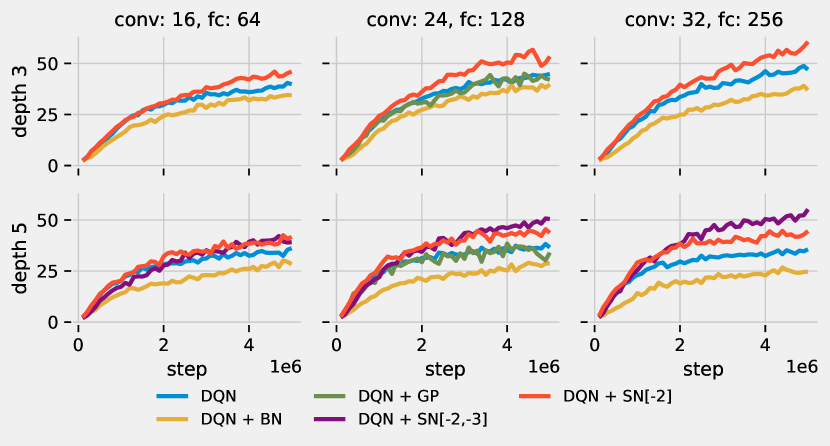
Figure 16: Regularization does not recover Spectral Normalization performance. Performance on MinAtar games of SN, GP and BN. Each line is an average over normalized scores of each game. Ten seeds for each configuration.

As briefly touched upon in Section 5.2, we investigated whether other regularisation methods imposing smoothness constraints can have similar effects on the agent’s performance. To this end we ran experiments with both Gradient Penalty (GP) and Batch Normalisation (BN) on several architectures (Table 6).

Batch Normalisation.

For each of the architectures we employed Batch Normalisation (BN) after the ReLU activation of every convolutional or linear layer except the output.

Gradient Penalty.

We did extensive experimentation and penalty coefficient tuning for Gradient Penalty regularisation. Specifically we tried penalising the norm of the sum of the gradients of all actions (the way GP is usually implemented in other domains), regularising the expected norm of each Q-value with respect to the state and also regularising the norm of the gradient of the Q-value associated with the optimal action. In all cases we swept through a wide range of penalty coefficients $\lambda$ with various degree of success. In Figure 16 we report the results of the best setting we could identify.

Relaxations to 1-Lipschitz normalisation.

We run a small experiment with a three layer network to investigate the relaxation introduced by (Gouk et al., 2020): $\mathbf{\hat{W}}_{i}=\mathbf{W}_{i}/\max(\lambda_{i},\lVert\mathbf{W}_{i}\rVert_{2})$. Figure 10 shows that for increased $\lambda_{i}$ values (which we keep equal for every layer) we are able to get good performance even when normalising all the layers of the network, further confirming our initial observation that controlling the amount of regularisation is important to achieving optimal performance and that achieving 1-Lipschitz functions is not critical in this setup. The increased computation required when approximating $\rho$ for all the layers and the addition of one hyper-parameter per layer determined us to not pursue this setup further.

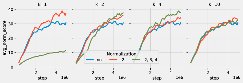
Figure 10: Relaxing the 1-Lipschitz condition recovers the performance for fully normalised networks. Average MinAtar Normalised Score of SN with different target Lipschitz constants. Each line is an average over normalised scores of 4 games $\times$ 10 seeds.

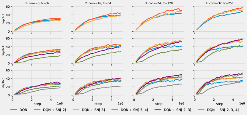
Figure 12: Spectral Normalization shows gains for all model sizes. Looking at the baseline ( DQN), we observe two performance regimes on MinAtar: for shallow, depth 3 models, performance increases with the width of the model; for deeper models performance generally stagnates with increasing depth and width. In both regimes applying SN on individual ( , ) or multiple ( ) layers improves upon the baseline suggesting a regularisation effect we could not reproduce with other regularisation methods. Notice that the strong regularisation resulted from applying SN to input layers ( ) or too many layers ( ) can however degrade performance. Each line is an average over normalized scores of 4 games $\times$ 10 seeds. Detailed view of Fig. 4.

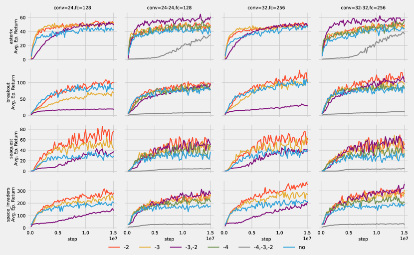
Figure 11: Performance curves of DQN agents using four different architectures trained for 15M steps. This plot shows that baseline plateaus, while spectrally normalised variants generally don’t. See Fig. 13 for plots of the spectral radii for the same experiments.

B.5 Adaptability to changing dynamics

We noticed that in most experiments on MinAtar the DQN agent reaches its peak performance within the standard 5M steps and then it plateaus. Most of these training curves end in flat performance regimes. In contrast, when SN is used on a single hidden layer, not only that agents surpass the baseline performance, but they also show continuous improvement with no signs of plateauing. We therefore asked what happens if we extend the training period and trained agents for 15M steps. As anticipated, our long training experiments show that SN agents show steep learning curves even after large numbers of steps (Fig. 11), supporting our claim that SN yields a better adapting optimiser.

B.6 Spectral Schedulers

For the experiments with the schedulers proposed in Sec. 5.4 we used the four estimator architectures in Table 6. We detail the MinAtar Normalised Score for various subsets of layers considered in the comparison in Figure 18. In a single subplot the lines represent the performance of the baseline, SN, and spectral schedulers, all using the same spectral radii. Observe that divOut has a close behaviour to that of SN not only on average, but also on a case base. In contrast, the mulEps and divGrad optimisers converge even when all hidden layers are normalised.

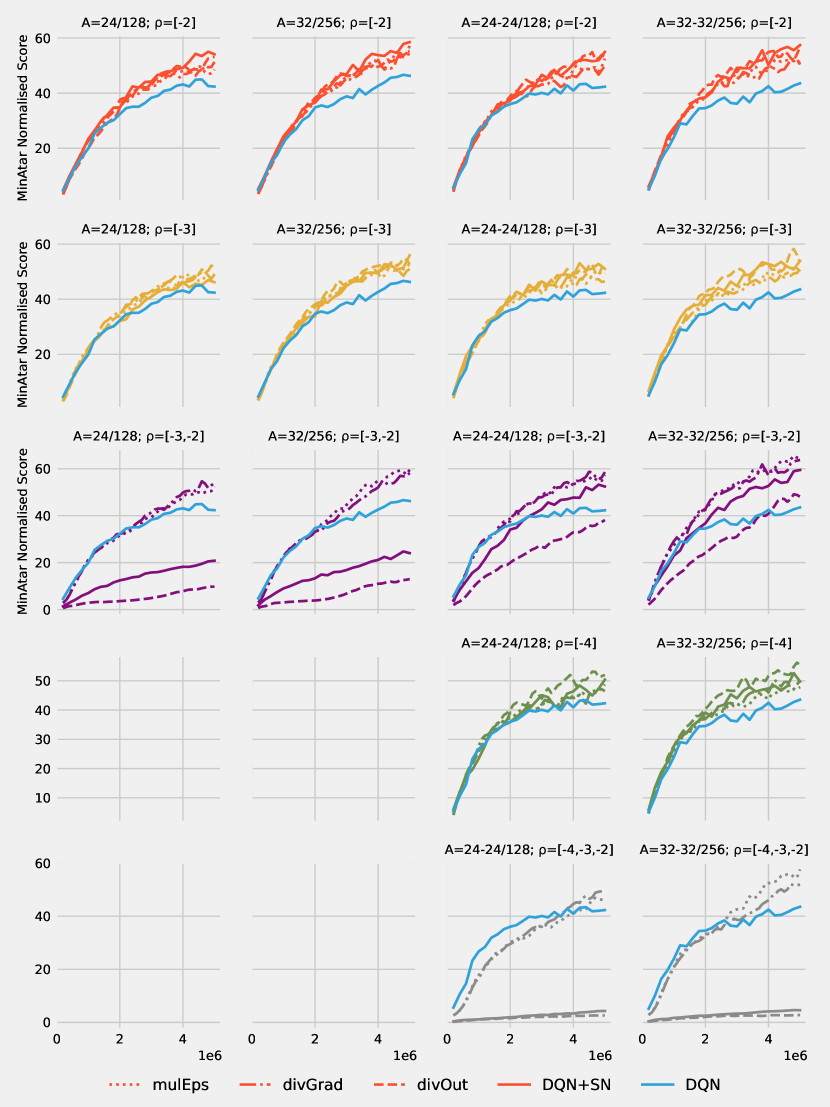
Figure 18: MinAtar Normalised Scored for the four architectures in Table 6 and various subsets of layers whose spectral radii are used for SN or spectral schedulers. Notice that divOut behaves similarly to SN (even when they fail to train), while mulEps and divGrad converge even when all hidden layers are normalised.

Experiment	No of conv layers	Conv width	FC width
Large optimisation sweep (B.1)	1 2 3 4 2 3	24 24 24 24 32 32	128 128 128 128 256 256
Regularisation (B.4)	1 3 1 3 1 3	16 16 24 24 32 32	64 64 128 128 256 256
Spectral schedulers (B.6) and long training run (B.5)	1 2 1 2	24 24 32 32	128 128 256 256

Table 6: Architecture sets used in the experiments described in this section.

Appendix C Atari experiments

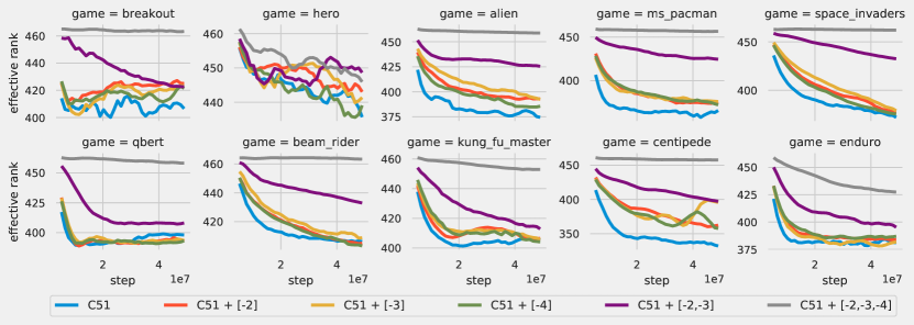
Figure 21: Spectral Normalisation preserves the Effective Rank of the features. Evolution of the effective rank of the features before the last linear layer of an C51 agent trained on 10 Atari games.

C.1 Evaluation protocols on Atari

In our work we mostly compare our Arcade Learning Environment (ALE) results with the Rainbow agent, therefore we adopt the evaluation protocol from (Hessel et al., 2018). Every 250K training steps in the environment we suspend the learning and evaluate the agent on 125K steps (or 500K frames). All the agents we train on ALE follow this validation protocol, the only difference being the validation epsilon value: $\epsilon=0.001$ for C51 and DQN-Adam which we directly compare to Rainbow and uses the same value and $\epsilon=0.05$ for DQN-RMSProp which follows the exact same hyper-parameters from (Mnih et al., 2015).

A major difference between the Rainbow protocol and the null op starts protocol used in earlier works is that in previous works the agent is evaluated for 30 or 100 (Van Hasselt et al., 2016) episodes and is allowed to play up to $18,000$ frames (5 minutes of emulator time) or by the end of the episode, whatever came first, whereas we always evaluate for up to $500,000$ frames.

Episodes are limited at 108K steps, the agent receives a game over signal when losing a life as in previous works and we use the null op starts to induce stochasticity in ALE games both at training and evaluation time (Van Hasselt et al., 2016).

C.2 DQN-Adam

Next, we wanted to showcase SN on an algorithm with a simpler objective such as DQN. However our initial experiments on MinAtar suggested that SN has a greater impact on Adam than on the RMSProp optimiser used in DQN (Mnih et al., 2015). Since we also wanted to be able to compare our results with those of Rainbow we use similar hyper-parameters to those in (Hessel et al., 2018). We list the full details in Table 7 especially since these hyper-parameters differ considerably from the the original DQN agent.

Hyper-parameter	Value
discount $\gamma$	0.99
update frequency	4
target update frequency	8000
starting $\epsilon$	1.0
final $\epsilon$	0.01
$\epsilon$ steps	250000
$\epsilon$ schedule	linear
warmup steps	20000
replay size	1M
batch size	32
history length	4
cost function	SmoothL1Loss
optimiser	Adam
learning rate $\eta$	0.00025
damping term $\epsilon$	0.0003125
$\beta_{1},\beta_{2}$	(0.9, 0.999)
validation steps	125000
validation $\epsilon$	0.001

Table 7: DQN-Adam hyper-parameters.

C.3 DQN - RMSprop

We also applied SN to a DQN agent optimised with RMSprop as in the original (Mnih et al., 2015). In conjunction with RMSprop the impact of SN seems minimal, far from the impressive improvement observed for the DQN-Adam agent. We leave for future work explaining the interaction between normalisation and RMSProp. See Table 8 for comparing the Human Normalised Score of DQN-RMSprop to other agents, and Fig. 22 for individual plots per game.

Agent	Mean	Median
DQN∗	357.36	102.94
DQN SN[-2]	375.37	105.19
DQN (Wang et al., 2016)	216.84	78.37
DQN-Adam∗	358.45	119.45
DQN-Adam SN[-2]	719.95	178.18

Table 8: Mean and median Human Normalised Score on 54 Atari games with random starts evaluation. References indicate the sources for the scores for each algorithm. We mark our own implementations of the baseline with $\ast$. Our agents are evaluated with the protocol in (Hessel et al., 2018). Note that the scores we report for our own implementation of DQN baseline are different from those reported in (Mnih et al., 2015) because the evaluation protocol has changed.

C.4 Effective rank

Authors of (Kumar et al., 2020) is making the case that for TD-learning with function approximation trained with SGD the neural network is being implicitly under-parametrised early in training. Empirically they show this by looking at the effective rank of the feature matrix $\bm{\Phi}$ which they approximate with the number of first $k$ singular values of $\bm{\Phi}$ that capture $99\%$ variance of all the singular values: $\sum_{i}^{k}\sigma_{i}(\bm{\Phi})\;/\;\sum_{j}^{d}\sigma_{j}(\bm{\Phi})\geq 0.99$. In this case the feature matrix $\bm{\Phi}$ is the input to the last linear layer in our neural network.

We perform their experiment, this time with a C51 agent with and without normalised layers looking to better understand the regularisation effects of normalisation. Figure 21 shows an evolution of the effective rank for the baseline agent that is consistent with the report of (Kumar et al., 2020). Interestingly, the baseline agent is consistently the one making use of fewer and fewer dimensions in the feature space as training progresses while the normalised agents preserve the rank. We further corroborate this finding with that of (Miyato et al., 2018) which is arguing that one of the possible disadvantages of Weight Normalisation (WN) as opposed to SN is that it prematurely producing sparse representations. Our experiments shows further shows that SN helps with preserving the rank of the features early on in training even when compared to an un-normalised agent.

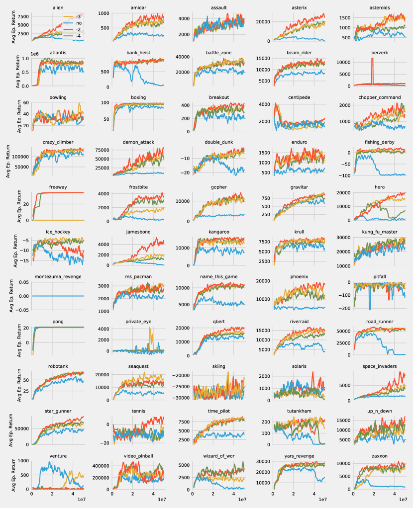
Figure 19: Performance curves of a DQN baseline optimised with Adam with SN applied on three different layers.

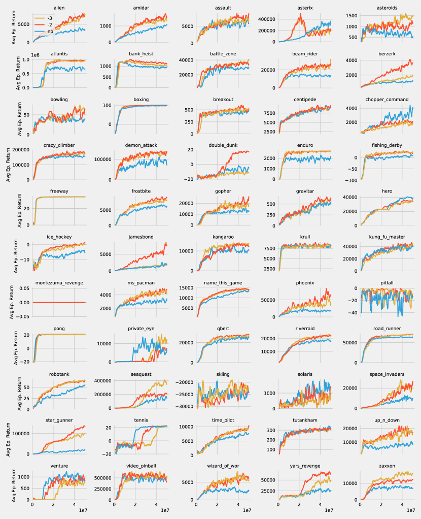
Figure 20: Performance curves of a C51 baseline with SN applied on three different layers.

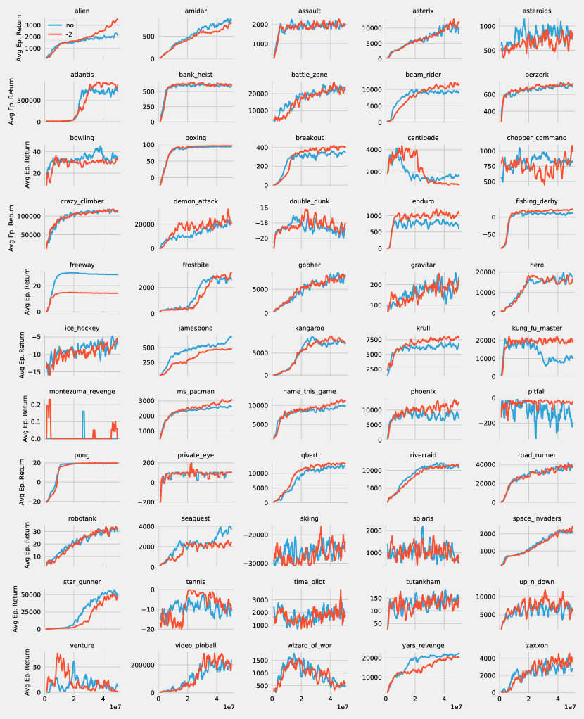
Figure 22: Performance curves of a DQN baseline optimised with RMSprop as in (Mnih et al., 2015) with SN applied on the penultimate layer.

References

- Anil et al. (2019) Anil, C., Lucas, J., and Grosse, R. Sorting out lipschitz function approximation. In International Conference on Machine Learning, pp. 291–301. PMLR, 2019.
- Arora et al. (2018) Arora, S., Li, Z., and Lyu, K. Theoretical analysis of auto rate-tuning by batch normalization. arXiv preprint arXiv:1812.03981, 2018.
- Bellemare et al. (2013) Bellemare, M. G., Naddaf, Y., Veness, J., and Bowling, M. The arcade learning environment: An evaluation platform for general agents. Journal of Artificial Intelligence Research, 47:253–279, 2013.
- Bellemare et al. (2017) Bellemare, M. G., Dabney, W., and Munos, R. A distributional perspective on reinforcement learning, 2017.
- Bengio et al. (2020) Bengio, E., Pineau, J., and Precup, D. Interference and generalization in temporal difference learning. ArXiv, abs/2003.06350, 2020.
- Bhatt et al. (2019) Bhatt, A., Argus, M., Amiranashvili, A., and Brox, T. Crossnorm: Normalization for off-policy td reinforcement learning. arXiv preprint arXiv:1902.05605, 2019.
- Castro et al. (2018) Castro, P. S., Moitra, S., Gelada, C., Kumar, S., and Bellemare, M. G. Dopamine: A research framework for deep reinforcement learning. arXiv preprint arXiv:1812.06110, 2018.
- Cissé et al. (2017) Cissé, M., Bojanowski, P., Grave, E., Dauphin, Y., and Usunier, N. Parseval networks: Improving robustness to adversarial examples. ArXiv, abs/1704.08847, 2017.
- Cobbe et al. (2019) Cobbe, K., Klimov, O., Hesse, C., Kim, T., and Schulman, J. Quantifying generalization in reinforcement learning. In ICML, 2019.
- Czarnecki et al. (2019) Czarnecki, W. M., Pascanu, R., Osindero, S., Jayakumar, S., Swirszcz, G., and Jaderberg, M. Distilling policy distillation. In The 22nd International Conference on Artificial Intelligence and Statistics, pp. 1331–1340. PMLR, 2019.
- Farnia et al. (2018) Farnia, F., Zhang, J. M., and Tse, D. Generalizable adversarial training via spectral normalization. arXiv preprint arXiv:1811.07457, 2018.
- Fortunato et al. (2018) Fortunato, M., Azar, M. G., Piot, B., Menick, J., Osband, I., Graves, A., Mnih, V., Munos, R., Hassabis, D., Pietquin, O., Blundell, C., and Legg, S. Noisy networks for exploration. ArXiv, abs/1706.10295, 2018.
- Givchi & Palhang (2014) Givchi, A. and Palhang, M. Quasi newton temporal difference learning. In ACML, 2014.
- Golub & van der Vorst (2000) Golub, G. H. and van der Vorst, H. A. Eigenvalue computation in the 20th century. Journal of Computational and Applied Mathematics, 123(1):35 – 65, 2000. ISSN 0377-0427. doi: https://doi.org/10.1016/S0377-0427(00)00413-1. URL http://www.sciencedirect.com/science/article/pii/S0377042700004131. Numerical Analysis 2000. Vol. III: Linear Algebra.
- Gouk et al. (2020) Gouk, H., Frank, E., Pfahringer, B., and Cree, M. J. Regularisation of neural networks by enforcing lipschitz continuity. Machine Learning, pp. 1–24, 2020.
- Gulrajani et al. (2017) Gulrajani, I., Ahmed, F., Arjovsky, M., Dumoulin, V., and Courville, A. C. Improved training of wasserstein gans. In Guyon, I., Luxburg, U. V., Bengio, S., Wallach, H., Fergus, R., Vishwanathan, S., and Garnett, R. (eds.), Advances in Neural Information Processing Systems, volume 30, pp. 5767–5777. Curran Associates, Inc., 2017. URL https://proceedings.neurips.cc/paper/2017/file/892c3b1c6dccd52936e27cbd0ff683d6-Paper.pdf.
- Henderson et al. (2018a) Henderson, P., Islam, R., Bachman, P., Pineau, J., Precup, D., and Meger, D. Deep reinforcement learning that matters. ArXiv, abs/1709.06560, 2018a.
- Henderson et al. (2018b) Henderson, P., Romoff, J., and Pineau, J. Where did my optimum go?: An empirical analysis of gradient descent optimization in policy gradient methods. ArXiv, abs/1810.02525, 2018b.
- Hessel et al. (2018) Hessel, M., Modayil, J., Hasselt, H. V., Schaul, T., Ostrovski, G., Dabney, W., Horgan, D., Piot, B., Azar, M. G., and Silver, D. Rainbow: Combining improvements in deep reinforcement learning. In AAAI, 2018.
- Hoffer et al. (2018) Hoffer, E., Banner, R., Golan, I., and Soudry, D. Norm matters: efficient and accurate normalization schemes in deep networks. arXiv preprint arXiv:1803.01814, 2018.
- Huster et al. (2018) Huster, T. P., Chiang, C. J., and Chadha, R. Limitations of the lipschitz constant as a defense against adversarial examples. In Nemesis/UrbReas/SoGood/IWAISe/GDM@PKDD/ECML, 2018.
- Ioffe & Szegedy (2015) Ioffe, S. and Szegedy, C. Batch normalization: Accelerating deep network training by reducing internal covariate shift. In International conference on machine learning, pp. 448–456. PMLR, 2015.
- Kingma & Ba (2014) Kingma, D. P. and Ba, J. Adam: A method for stochastic optimization. arXiv preprint arXiv:1412.6980, 2014.
- Kumar et al. (2020) Kumar, A., Agarwal, R., Ghosh, D., and Levine, S. Implicit under-parameterization inhibits data-efficient deep reinforcement learning. arXiv preprint arXiv:2010.14498, 2020.
- Kunstner et al. (2019) Kunstner, F., Hennig, P., and Balles, L. Limitations of the empirical fisher approximation for natural gradient descent. In Wallach, H., Larochelle, H., Beygelzimer, A., d'Alché-Buc, F., Fox, E., and Garnett, R. (eds.), Advances in Neural Information Processing Systems, volume 32, pp. 4156–4167. Curran Associates, Inc., 2019. URL https://proceedings.neurips.cc/paper/2019/file/46a558d97954d0692411c861cf78ef79-Paper.pdf.
- Kurach et al. (2019) Kurach, K., Lučić, M., Zhai, X., Michalski, M., and Gelly, S. A large-scale study on regularization and normalization in gans. In International Conference on Machine Learning, pp. 3581–3590. PMLR, 2019.
- Liu et al. (2020) Liu, J. Z., Lin, Z., Padhy, S., Tran, D., Bedrax-Weiss, T., and Lakshminarayanan, B. Simple and principled uncertainty estimation with deterministic deep learning via distance awareness. arXiv preprint arXiv:2006.10108, 2020.
- Liu et al. (2019) Liu, Z., Li, X., Kang, B., and Darrell, T. Regularization matters in policy optimization – an empirical study on continuous control, 2019.
- Machado et al. (2018) Machado, M. C., Bellemare, M. G., Talvitie, E., Veness, J., Hausknecht, M., and Bowling, M. Revisiting the arcade learning environment: Evaluation protocols and open problems for general agents. Journal of Artificial Intelligence Research, 61:523–562, 2018.
- Martens (2010) Martens, J. Deep learning via hessian-free optimization. In ICML, volume 27, pp. 735–742, 2010.
- Martens & Grosse (2015) Martens, J. and Grosse, R. Optimizing neural networks with kronecker-factored approximate curvature. In International conference on machine learning, pp. 2408–2417. PMLR, 2015.
- Miyato et al. (2018) Miyato, T., Kataoka, T., Koyama, M., and Yoshida, Y. Spectral normalization for generative adversarial networks, 2018.
- Mnih et al. (2015) Mnih, V., Kavukcuoglu, K., Silver, D., Rusu, A. A., Veness, J., Bellemare, M. G., Graves, A., Riedmiller, M., Fidjeland, A. K., Ostrovski, G., et al. Human-level control through deep reinforcement learning. nature, 518(7540):529–533, 2015.
- Obando-Ceron & Castro (2020) Obando-Ceron, J. S. and Castro, P. S. Revisiting rainbow: Promoting more insightful and inclusive deep reinforcement learning research. ArXiv, abs/2011.14826, 2020.
- Osband et al. (2016) Osband, I., Blundell, C., Pritzel, A., and Roy, B. V. Deep exploration via bootstrapped dqn. In NIPS, 2016.
- Pascanu & Bengio (2014) Pascanu, R. and Bengio, Y. Revisiting natural gradient for deep networks. In International Conference on Learning Representations 2014 (Conference Track), April 2014. URL http://arxiv.org/abs/1301.3584.
- Romoff et al. (2020) Romoff, J., Henderson, P., Kanaa, D., Bengio, E., Touati, A., Bacon, P., and Pineau, J. Tdprop: Does jacobi preconditioning help temporal difference learning? ArXiv, abs/2007.02786, 2020.
- Rosca et al. (2020) Rosca, M., Weber, T., Gretton, A., and Mohamed, S. A case for new neural network smoothness constraints, 2020.
- Salimans & Kingma (2016) Salimans, T. and Kingma, D. P. Weight normalization: A simple reparameterization to accelerate training of deep neural networks. arXiv preprint arXiv:1602.07868, 2016.
- Santurkar et al. (2018) Santurkar, S., Tsipras, D., Ilyas, A., and Madry, A. How does batch normalization help optimization? In Advances in neural information processing systems, pp. 2483–2493, 2018.
- Schaul et al. (2016) Schaul, T., Quan, J., Antonoglou, I., and Silver, D. Prioritized experience replay. CoRR, abs/1511.05952, 2016.
- Sun et al. (2020) Sun, T., Shen, H., Chen, T., and Li, D. Adaptive temporal difference learning with linear function approximation. arXiv preprint arXiv:2002.08537, 2020.
- Tieleman & Hinton (2012) Tieleman, T. and Hinton, G. Lecture 6.5—RmsProp: Divide the gradient by a running average of its recent magnitude. COURSERA: Neural Networks for Machine Learning, 2012.
- Toromanoff et al. (2019) Toromanoff, M., Wirbel, E., and Moutarde, F. Is deep reinforcement learning really superhuman on atari? leveling the playing field, 2019.
- Tsuzuku et al. (2018) Tsuzuku, Y., Sato, I., and Sugiyama, M. Lipschitz-Margin Training: Scalable Certification of Perturbation Invariance for Deep Neural Networks. In Bengio, S., Wallach, H., Larochelle, H., Grauman, K., Cesa-Bianchi, N., and Garnett, R. (eds.), Advances in Neural Information Processing Systems 31, pp. 6542–6551. Curran Associates, Inc., 2018.
- Van Hasselt et al. (2016) Van Hasselt, H., Guez, A., and Silver, D. Deep reinforcement learning with double q-learning. In Proceedings of the AAAI conference on artificial intelligence, volume 30, 2016.
- Van Laarhoven (2017) Van Laarhoven, T. L2 regularization versus batch and weight normalization. arXiv preprint arXiv:1706.05350, 2017.
- Virmaux & Scaman (2018) Virmaux, A. and Scaman, K. Lipschitz regularity of deep neural networks: analysis and efficient estimation. In Bengio, S., Wallach, H., Larochelle, H., Grauman, K., Cesa-Bianchi, N., and Garnett, R. (eds.), Advances in Neural Information Processing Systems, volume 31, pp. 3835–3844. Curran Associates, Inc., 2018. URL https://proceedings.neurips.cc/paper/2018/file/d54e99a6c03704e95e6965532dec148b-Paper.pdf.
- Wang et al. (2016) Wang, Z., Schaul, T., Hessel, M., Hasselt, H., Lanctot, M., and Freitas, N. Dueling network architectures for deep reinforcement learning. In International conference on machine learning, pp. 1995–2003. PMLR, 2016.
- Yoshida & Miyato (2017) Yoshida, Y. and Miyato, T. Spectral norm regularization for improving the generalizability of deep learning. ArXiv, abs/1705.10941, 2017.
- Young & Tian (2019) Young, K. and Tian, T. Minatar: An atari-inspired testbed for thorough and reproducible reinforcement learning experiments. arXiv preprint arXiv:1903.03176, 2019.
- Yu et al. (2020) Yu, T., Thomas, G., Yu, L., Ermon, S., Zou, J., Levine, S., Finn, C., and Ma, T. Mopo: Model-based offline policy optimization, 2020.