Outlier Detection for Functional Data with R Package fdaoutlier

Oluwasegun Ojo, Rosa E. Lillo, Antonio Fernandez-Anta Outlier Detection for Functional Data with R Package fdaoutlier Outlier detection is one of the standard exploratory analysis tasks in functional data analysis. We present the R package fdaoutlier which contains implementations of some of the latest techniques for detecting functional outliers. The package makes it easy to detect different types of outliers (magnitude, shape, and amplitude) in functional data, and some of the implemented methods can be applied to both univariate and multivariate functional data. We illustrate the main functionality of the R package with common functional datasets in the literature. functional data analysis, outlier detection, fdaoutlier, R functional data analysis, outlier detection, fdaoutlier, R Oluwasegun Ojo
Global Computing Group
IMDEA Networks Institute
and
Universidad Carlos III de Madrid
E-mail:
URL: https://statimatics.com/about

1 Introduction

Outlier detection is a common task when carrying out exploratory data analysis. Identifying possible outliers is essential during the exploratory analysis process, because outliers can significantly bias any statistical analysis. The process of dealing with identified outliers may also provide new insights into the data generating process’s nature. In functional data analysis (FDA), observations are treated as functions observed on a domain. These functional observations can exhibit various outlyingness properties as pointed out by hubert2015multivariate. For instance, an observation can be shifted from the mass of the data. Such outliers are referred to as magnitude outliers in the FDA literature. On the other hand, an observation can be a shape outlier because it differs in shape from the mass of the data (even if it lies completely inside the mass of the data). For periodic functional observations, an observation may be outlying because it has an amplitude different from the mass of the data. Finally, any of the aforementioned outlyingness properties can be exhibited by a functional observation in a subset of the domain or all through the domain. Consequently, identifying outliers in FDA is challenging as there are many possible ways a functional observation can exhibit outlyingness.

Much work has been done regarding identifying outliers in the FDA context, with their corresponding software implementations made available in R (Rcore). A number of these methods have been obvious applications of a notion of functional depths, which induces a centre outward ordering on a sample of curves. For instance, the functional boxplot (sun2011functional) uses the (modified) band depth to define a 50% central region for the sample of curves with outliers identified as curves lying outside 1.5 times the central region in any part of the domain. In R, the functional boxplot is available in the fda package (fdapackage) with options to use the fast exact (modified) band depth defined by bands of two functions, proposed in sun2012exact.

The fda.usc package (fda.usc) in R implements three functional outlier detection methods. The first method, proposed in febrero2007functional, uses a likelihood ratio statistics to detect outlying curves (with cutoff determined by a bootstrap procedure). The two other methods identify outliers by comparing the depth values of the functions to a cutoff also obtained by a bootstrap procedure, based on either trimming of suspicious curves or placing more weights on the deeper curves (febrero2008). These three methods are also implemented in the rainbow package (hanlinshang2011rj), as well as the functional bagplot and the functional highest density region plot (hyndman2010bagplot). The rainbow package also contains the integrated square forecast errors method for detecting functional outliers proposed in hyndmanullah2018 (see also hyndman2010bagplot).

nagy07depth proposed the $j^{th}$ order integrated and infimal depths for identifying shape outliers, with implementations available in the ddalpha package (pokotylo2019ddalpha). rousseeuw2018measure in their work proposed a directional outlyingness (DO) measure, its functional extension (fDO), and the variability of directional outlyingness (vDO). Then, they used the functional outlier map, a scatter plot of the fDO versus vDO, to identify outliers with cutoffs determined by the standardized logarithm of the combined functional outlyingness(LCFO) measure. The functional outlier map can also be used with the adjusted outlyingness (AO) measure proposed in brys2005robustification (see also hubert2008outlier, and hubert2015multivariate hubert2015multivariate), rather than the DO measure. These methods are available in the mrfDepth package (mrfdepth). Finally, the roahd package (ieva2019roahd) contains an implementation of the outliergram method proposed in arribas2014shape, as well as its multivariate generalisation proposed in ieva2020component.

More recently proposed outlier detection methods include: the directional outlyingness for multivariate functional data proposed in dai2019directional and further elaborated into the magnitude-shape plot (MS-Plot) in dai2018multivariate; the total variate depth (TVD) and modified shape similarity index (MSS) proposed in huang2019decomposition; and the CRO-FADALARA method, based on archetypoids proposed in vinue2020robust, and available in the adamethods package (ada). dai2020sequential also proposed detecting and classifying outliers using some sequence of transformations, e.g., shifting a curve to its centre and normalising it using the $L_{2}$ norm.

The objective of this paper is to describe the fdaoutlier package which aims to extend the available facility for outlier detection (in the FDA context) for R, with implementations of some of the latest outlier detection methods. The fdaoutlier package’s main contributions are:

• Implementations of the directional outlyingness and MS-Plot outlier detection methods proposed in dai2019directional and dai2018multivariate.

• An implementation of the TVD and MSS proposed in huang2019decomposition. The fdaoutlier implementation of TVD/MSS is written in C++ using R’s .Call interface which leads to significant computational efficiency as TVD and MSS are computationally intensive.

• An implementation of the sequential tranformation method described in dai2020sequential.

• An implementation of the massive unsupervised outlier detection (MUOD) method proposed in azcorra2018unsupervised.

• Various depth and ordering methods, including extremal depth, one and two-sided extreme rank length depth, directional quantile, among others, useful for ordering functional observations (e.g., in functional boxplots).

In the next section, we describe the theoretical background of the implemented outlier detection methods and demonstrate their implementations in fdaoutlier using simulated data. In Section 3, we apply fdaoutlier on two common datasets in the FDA outlier detection literature, replicating some of the analyses done in the literature. We then conclude in Section 4 with some remarks and a future outlook of fdaoutlier.

2 Outlier detection methods

We provide a brief primer of the implemented methods in the fdaoutlier package, and then describe their implementations. For illustrating the methods, we use the convenience functions simulation_model1() - simulation_model9() implemented in fdaoutlier to generate data with different types of outliers. These functions are useful for the rapid development and testing of new outlier detection methods and were curated from the functional outlier detection literature. Figure 1 shows plots of sample data generated by these nine models produced by calling simulation_model*(plot = TRUE).

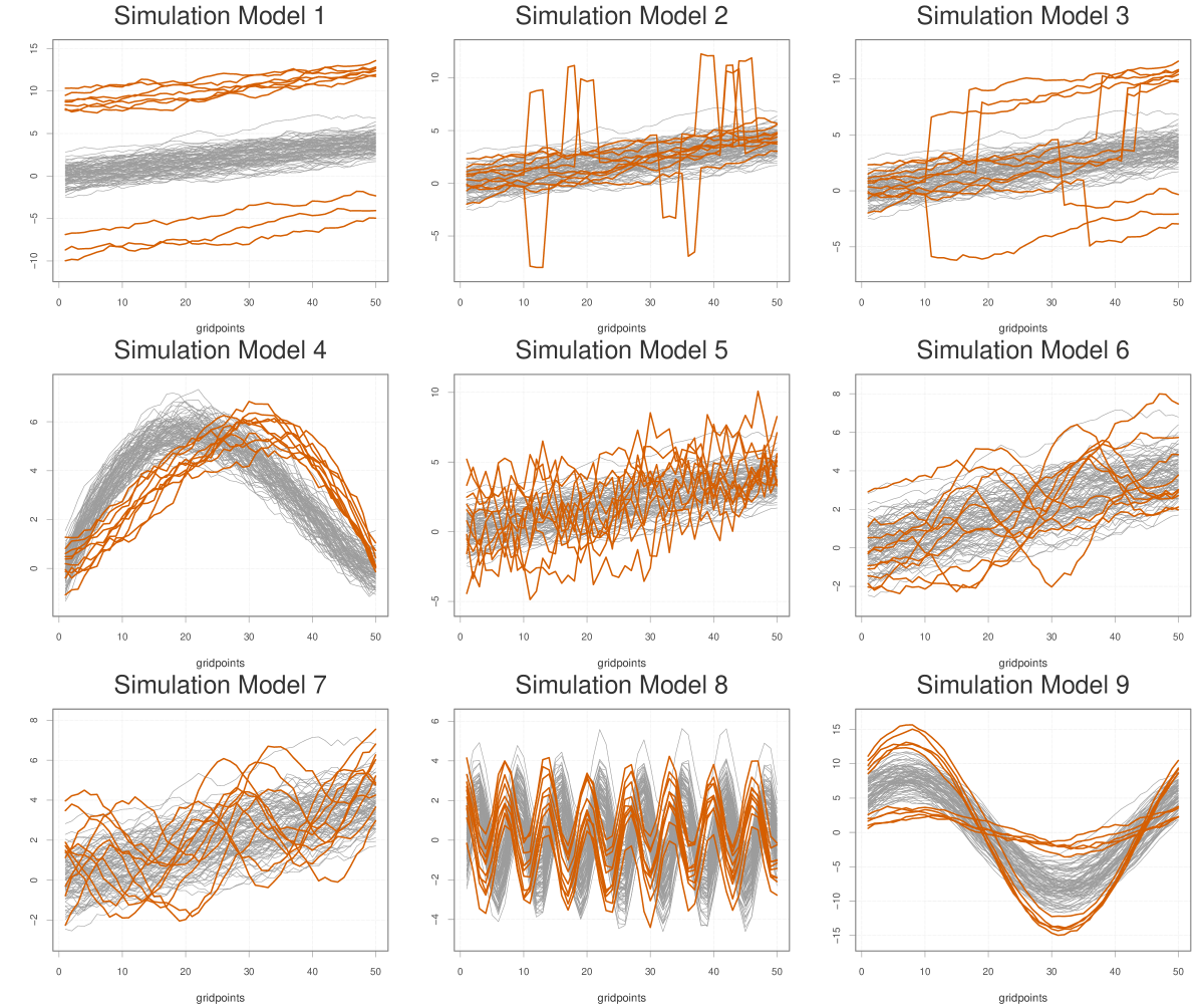
Figure 1: Simulation models: Plot of sample of data generated by each simulated model in fdaoutlier. Curves in orange are outliers.

2.1 Directional outlyingness and MS-Plot

The directional outlyingess for multivariate functional data proposed in dai2019directional provides a way to measure not only the point-wise outlyingness of a functional observations but also the direction of outlyingness of that observation with respect to (w.r.t.) the rest of the data. Formally, let $\textbf{Y}:I\rightarrow\mathbb{R}^{p}$ be a stochastic process in the space of real continuous functions $C(I,\mathbb{R}^{p})$ defined on a compact interval $I$. Let the probability distribution of Y be $F_{\textbf{Y}}$. At each evaluation point, $t\in I$, $\textbf{Y}(t)$ is a $p$-variate vector with probability distribution $F_{\textbf{Y}(t)}$. The directional outlyingness for multivariate data is defined as:

$$\textbf{O}(\textbf{Y},F_{\textbf{Y}})=o(\textbf{Y},F_{\textbf{Y}})\cdot\textbf{v},$$ (1)

where $o(\textbf{Y},F_{\textbf{Y}})$ is the outlyingness of Y w.r.t. to $F_{\textbf{Y}}$ and v is the spatial depth defined at point $t$ by

$$\textbf{v}(t)=\frac{|\textbf{Y}(t)-\textbf{Z}(t)|}{||\textbf{Y}(t)-\textbf{Z}(t)||},$$ (2)

with $\textbf{Z}(t)$ being the unique median of $\textbf{Y}(t)$ w.r.t. $F_{\textbf{Y}(t)}$ (deepest point of $F_{\textbf{Y}(t)}$). $\textbf{v}(t)$ is a unit vector pointing from $\textbf{Z}(t)$ to $\textbf{Y}(t)$. dai2019directional recommends using a distance-based outlyingness measure, like the Stahel-Donoho outlyingness defined by:

$$\mathit{SDO}(\textbf{Y}(t),F_{\textbf{Y}(t)})=\sup\limits_{||\textbf{u}||=1}\frac{||\textbf{u}^{\top}\textbf{Y}(t)-\text{median}(\textbf{u}^{\top}\textbf{Y}(t))||}{\text{mad}(\textbf{u}^{\top}\textbf{Y}(t))}.$$ (3)

Thus, the Stahel-Donoho type directional outlyingness is given by:

$$\textbf{O}(\textbf{Y},F_{\textbf{Y}})=\mathit{SDO}(\textbf{Y},F_{\textbf{Y}})\cdot\textbf{v}.$$ (4)

Then the functional directional outlyingness (FO) is defined, to capture the overall outlyingness for functional data, as:

$$\text{FO}(\textbf{Y},F_{\textbf{Y}})=\int_{I}||\textbf{O}(\textbf{Y}(t),F_{\textbf{Y}(t)})||^{2}w(t)dt,$$ (5)

where $w(t)$ is a weight function defined on $I$. The mean directional outlyingness (MO) and variation of directional outlyingness (VO) were defined as :

$$\textbf{MO}(\textbf{Y},F_{\textbf{Y}})=\int_{I}\textbf{O}(\textbf{Y}(t),F_{\textbf{Y}(t)})w(t)dt,$$ (6)

and

$$\text{VO}(\textbf{Y},F_{\textbf{Y}})=\int_{I}||\textbf{O}(\textbf{Y}(t),F_{\textbf{Y}(t)})-\textbf{MO}(\textbf{Y},F_{\textbf{Y}})||^{2}w(t)dt.$$ (7)

These quantities measure the magnitude outlyingness and shape outlyingness of a functional observation, respectively. dai2019directional further showed the relationship:

$$\text{FO}(\textbf{Y},F_{\textbf{Y}})=||\textbf{MO}(\textbf{Y},F_{\textbf{Y}})||^{2}+\text{VO}(\textbf{Y},F_{\textbf{Y}}),$$ (8)

which decomposes the total functional outlyingness into the magnitude outlyingness and the shape outlyingness.

In practice, the functional observations are obseved at a finite number of points, say $k$, on $I$, i.e., at points $t_{1},t_{2},\ldots,t_{k}\in I$. The finite dimensional version of $\textbf{MO}(\textbf{Y},F_{\textbf{Y}})$ is defined as:

$$\textbf{MO}_{k}(\textbf{Y},F_{\textbf{Y}})=\frac{1}{k}\sum\limits_{i=1}^{k}\textbf{O}(\textbf{Y}(t_{i}),F_{\textbf{Y}(t_{i})})w(t_{i}),$$ (9)

and the finite dimensional version of VO can defined in a similar manner.

After obtaining the MO and VO for each curve, MS-Plot is then a scatterplot of the points $(\textbf{MO}^{\top},\text{VO})^{\top}$. To detect outliers, a multivariate data whose columns are the MOs and VOs is formed, and a robust Mahalanobis distance is computed for each of the $(\textbf{MO}^{\top},\text{VO})^{\top}$ pair in this data. The robust covariance matrix is estimated using the minimum covariate determinant (MCD) estimator (rousseeuw1999fast). The distribution of these robust distances is approximated using the F distribution (hardinrocke3005). Any observation with a robust distance greater than the cutoff obtained from the tails of the F distribution is flagged as an outlier.

The directional outlyingness and MS-Plot methods procedures are implemented mainly through the dir_out() and msplot() functions in fdaoutlier. These functions accept a matrix or data frame of dimension $n\times p$ for a univariate functional data, or an array of dimension $n\times p\times d$ for multivariate functional data (where $n$ is the number of functions/curves, $p$ is the number of evaluation points in the domain, and $d$ is the dimension of the functional data with, $d\geq 2$ for multivariate functional data). The dir_out() function computes the directional outlyingness matrix $\textbf{O}(\textbf{Y},F_{\textbf{Y}})$, the mean directional outlyingness $\textbf{MO}(\textbf{Y},F_{\textbf{Y}})$ and the variation of directional $\text{VO}(\textbf{Y},F_{\textbf{Y}})$, while the msplot() function finds outliers using the mean and variation of outlyingness with the F approximation.

We illustrate identifying outliers with msplot() using simulation_model5() to generate data of 100 curves, out of which 10 are shape outliers with a different covariance structure. The generated curves are observed on 50 domain points over the interval $[0,1]$. A call to simulation_model5() returns a list containing the matrix of generated data and a vector containing the indices of the true outliers. R> simdata <- simulation_model5(n = 100, p = 50, + outlier_rate = 0.1, seed = 2) R> dt <- simdata$dataR>dim(dt)\Soutput[1]10050\Sinput R>simdata$true_{o}utliers\Soutput[1]6102021343848496693Nextwepassthegenerateddatatothe\code{msplot()}functiontodetecttheoutliersin\code{dt}.Bydefault,\code{msplot()}alsoproducesaplotoftheVOagainsttheMO(or$||MO ||$inthecaseofamultivariatefunctionaldata)andreturnsalistcontaining\code{outliers}whichisavectoroftheindicesofdetectedoutliers.Theplottingfunctioncanbeturnedoffbysettingtheparameter\code{plot=FALSE}.\Schunk\Sinput R>ms<-msplot(dts=dt,return_{m}vdir=T,plot=FALSE)R>ms$outliers\Soutput[1]610202134384849516693100Settingtheadditionalparameter\code{return_{m}vdir=TRUE}ensuresthatvectorsofthemeanandvariationofoutlyingness(MOandVO)ofeachcurvearereturnedby\code{msplot()}(amatrixisreturnedfor\textbf{MO}inthecaseofamultivariatefunctionaldata).\Schunk\Sinput R>head(ms$mean_{o}utlyingness)\Soutput[1]0.04718408-0.761346121.305028070.204141530.81537363[6]2.27956644\Sinput R>head(ms$var_{o}utlyingness)\Soutput[1]0.21158060.17774220.20153000.38986910.15506512.2730378\begin{figure}[t!]\centering\includegraphics{article-msplot1}\@@toccaption{{\lx@tag[ ]{{2}}{MS-Plot:PlotoftheVOagainsttheMO.}}}\@@caption{{\lx@tag[: ]{{Figure 2}}{MS-Plot:PlotoftheVOagainsttheMO.}}}\@add@centering\end{figure}\par TheMS-Plotproducedbythe\code{msplot()}functionwhentheparameter\code{plot=TRUE}isshowninFigure~{}\ref{fig:msplot}.Additionalparameters\code{plot_{t}itle},\code{title_{c}ex},\code{show_{l}egend},\code{ylabel}and\code{xlabel}canbepassedto\code{msplot()}tofurthercustomisetheMS-Plotgenerated.\par IftheaimistocomputeeithertheMOandVOorthedirectionaloutlyingnessmatrix(orarrayformultivariatefunctionaldata),withouttheneedforidentifyingoutliers,thenthe\code{dir_{o}ut()}function,whichiscalledby\code{msplot()}canbeuseddirectly.Thisreturnsalistcontainingthemeanandvarianceofoutlyingness,andthedirectionaloutlyingnessmatrix(iftheparameter\code{return_{d}ir_{m}atrix=TRUE}).\Schunk\Sinput R>simdir<-dir_{o}ut(dts=dt,return_{d}ir_{m}atrix=T)R>head(simdir$mean_{o}utlyingness)\Soutput[1]0.04718408-0.761346121.305028070.204141530.81537363[6]2.27956644\Sinput R>head(simdir$var_{o}utlyingness)\Soutput[1]0.21158060.17774220.20153000.38986910.15506512.2730378\Sinput R>dim(simdir$dirout_{m}atrix)\Soutput[1]10050$

2.2 Total variation depth and modified shape similarity index

Suppose $Y:I\rightarrow\mathbb{R}$ is a stochastic process defined on the interval $I$ in $\mathbb{R}$. Let the distribution of $Y$ be $F_{Y}$. For a function $y$, let $R_{y}(t)$ be the indicator function:

$$R_{y}(t)=\mathbbm{1}\{Y(t)\leq y(t)\},$$ (10)

for $t\in I$. The functional total variation depth (huang2019decomposition) of the function $y$ w.r.t. $F_{Y}$ is then defined as:

$$\mathit{TVD}(y,F_{Y})=\int_{I}D_{y}(t)w(t)dt,$$ (11)

where $w(t)$ is a weight function and $D_{y}(t)$ is the pointwise total variation depth given by:

$$D_{y}(t)=\textrm{var}\{R_{y}(t)\}=\mathbb{P}\{Y(t)\leq y(t)\}\mathbb{P}\{Y(t)>y(t)\}.$$ (12)

The constant weight function $w(t)=\frac{1}{|I|}$ is suggested in (huang2019decomposition) but other weight functions (that place more emphasis on different regions of the interval) can be used in the formulation of the functional total variation depth. The pointwise total variation depth $D_{y}(t)$ can be decomposed into a shape and magnitude component by breaking up the variance $\textrm{var}\{R_{y}(t)\}$ using the law of total variance:

$$D_{y}(t)=\textrm{var}\{R_{y}(t)\}=\textrm{var}[\mathbb{E}\{R_{y}(t)|R_{y}(s)\}]+\mathbb{E}[\textrm{var}\{R_{y}(t)|R_{y}(s)\}],$$ (13)

for $s,t\in I$ and $s=t-\Delta$. The shape similarity index of the functional observation $y$ in a given time span $\Delta$ is then the weighted ratio of the shape component $\textrm{var}[\mathbb{E}\{R_{y}(t)|R_{y}(s)\}]$ to the total variation depth over the interval $I$:

$$\mathit{SS}(y,\Delta)=\int_{I}S_{y}(t,\Delta)v(t,\Delta)dt,$$ (14)

where

$$S_{y}(t,\Delta)=\begin{cases}\textrm{var}[\mathbb{E}\{R_{y}(t)|R_{y}(s)\}]/D_{y}(t)&D_{y}(t)\neq 0\\ 1&D_{y}(t)=0,\\ \end{cases}$$

and the weight function $v(t,\Delta)$ is the normalised changes in $y(t)$ over the interval $I$:

$$v(t,\Delta)=\frac{|y(t)-y(t-\Delta)|}{\int_{I}|y(t)-y(t-\Delta)|}.$$

The shape similarity index is a measure of shape outlyingness with small indices associated with shape outliers. However, when $D_{y}(t)$ is very small, the shape similarity index may not be small enough, so huang2019decomposition further defined the modified shape similarity index (MSS) by shifting $(y(t-\Delta),y(t))$ to the centre. The modified shape similarity index is defined as:

$$\mathit{MSS}(y,\Delta)=\int_{I}S_{\tilde{y}}(t,\Delta)v(t,\Delta)dt,$$ (15)

where $\widetilde{y}$ is given by:

$$\widetilde{y}(s,\Delta)=\begin{cases}\textrm{median}\{Y(s)\}&s=t\\ f(s)-f(s+\Delta)+\textrm{median}[Y(s+\Delta)]&s=t-\Delta,\end{cases}$$

and

$$S_{\tilde{y}}(t,\Delta)=\textrm{var}(\mathbb{E}[R_{\tilde{y}}(t)|R_{\tilde{y}}(s)])/D_{\tilde{y}}(t)\}.$$

Details of the empirical versions of the total variation depth, the shape similarity index and its modified version are presented in the Appendix of huang2019decomposition. The total variation depth and the modified similarity index are implemented in the total_variation_depth() function of fdaoutlier using C++ through R’s .Call interface for faster and efficient computation. This function accepts only a matrix, and calling it suffices to compute both the total variation depth and the modified shape similarity index. total_variation_depth() returns a list containing both the total variation depth and the modified shape similarity index: R> tvdepth <- total_variation_depth(dt) R> head(tvdepth$mss)\Soutput[1]0.63882170.62086590.69752330.68536330.66183130.2167154\Sinput R>head(tvdepth$tvd)\Soutput[1]0.2245780.1564840.1143860.1979320.1789260.072398Inordertoidentifyoutliers,shapeoutliersarefirstidentifiedandremovedusingaclassicalboxplotonthemodifiedshapesimilarityindices.Afunctionalboxplotisthenusedontheremainingcurves(toidentifymagnitudeoutliers)usingthetotalvariationdepthtoidentifytheir$50%$centralregion(relativetotheoriginalnumberofcurves).The\code{tvdmss()}functionimplementsthesestepstodetectthemagnitudeandshapeoutliers.Itreturnsafunctioncontainingtheindicesofthemagnitudeoutliers,shapeoutliers,andthecombined(shapeandmagnitude)outliers.Thisisillustratedusingthegenerateddata\code{dt}fromtheprevioussection.\Schunk\Sinput R>tvoutlier<-tvdmss(dts=dt)R>tvoutlier$shape_{o}utliers\Soutput[1]6102021343848496693\Sinput R>tvoutlier$magnitude_{o}utliers\Soutput NULL\Sinput R>tvoutlier$outliers\Soutput[1]6102021343848496693Inthiscasethetotalvariationdepthidentifiesalltheshapeoutlierscorrectlyanddoesnotdetectanymagnitudeoutlierswhencomparedtotheindexofthetrueoutliersofthegenerateddata:\par\Schunk\Sinput R>simdata$true_{o}utliers\Soutput[1]6102021343848496693\par Additionalargumentscanbepassedtotheparameters\code{emp_{f}actor_{m}ss},\code{emp_{f}actor_{t}vd},and\code{central_{r}egion_{t}vd}of\code{tvdmss()}tocontroltheclassicalboxplotofthemodifiedshapesimilarityindexandthefunctionalboxplotofthetotalvariationdepth.\par$

2.3 Outlier detection using sequential transformations

dai2020sequential proposed using some sequence of tranformations on the functional data to identify and classify functional outliers. By transforming the functional data, it is possible to turn shape outliers into magnitude outliers, consequently making it easier to identify shape outliers. More formally, let $\{Y_{i}\}_{i=1}^{n}$ be a set of functional observations in the space of continous functions $C(I)$ defined on an interval $I\in\mathbb{R}$. Suppose that $Y_{i}\sim F_{Y}$, and let $\Gamma$ be a transformation that is also defined on $C(I)$. Furthermore, let $F_{\Gamma(Y)}$ be the distribution of the transformed data $\{\Gamma(Y_{i})\}_{i=1}^{n}$. dai2020sequential proposed the following algorithm for functional outlier detection and taxonomy.

1 Identify from $\{Y_{i}\}_{i=1}^{n}$ the magnitude outliers using the functional boxplot, and denote the set of identified outliers by $S_{0}$. These are the $\Gamma_{0}-$outliers (magnitude outliers).

2 Apply transformation $\Gamma_{1}$ on $\{Y_{i}\}_{i=1}^{n}$ to get $\{\Gamma_{1}(Y_{i})\}_{i=1}^{n}$.

3 Repeat step 1 on $\{\Gamma_{1}(Y_{i})\}_{i=1}^{n}$ to obtain the set of detected outliers $S_{1}$; $S_{1}\setminus S_{0}$ are the $\Gamma_{1}-$shape outliers.

4 Apply transformation $\Gamma_{2}$ on $\{\Gamma_{1}(Y_{i})\}_{i=1}^{n}$ to get $\{\Gamma_{2}\circ\Gamma_{1}(Y_{i})\}_{i=1}^{n}$.

5

6Repeat step 1 on $\{\Gamma_{2}\circ\Gamma_{1}(Y_{i})\}_{i=1}^{n}$ to obtain the set of detected outliers $S_{2}$; $S_{2}\setminus S_{1}\cup S_{0}$ are the $\Gamma_{2}\circ\Gamma_{1}-$shape outliers.

7

8Repeat steps 4 and 5 if more transformations are considered.

Algorithm 1 Functional outlier detection using sequential transformations.

dai2020sequential proposed the following useful (sequence of) transformations to identify and classify outliers:

Shifting and normalization of Curves: $\mathcal{T}_{2}\circ\mathcal{T}_{1}\circ\mathcal{T}_{0}(Y_{i})$

This sequence involves first identifying the magnitude outliers using functional boxplot. This is the $\mathcal{T}_{0}$ transformation and the identified outliers are the $\mathcal{T}_{0}$ outliers (magnitude outliers). The second transformation $\mathcal{T}_{1}$ involves shifting the raw curves $Y_{i}$ to their centres:

$$\mathcal{T}_{1}(Y)(t)=Y(t)-\lambda(I)^{-1}\int_{I}Y(t)dt,$$ (16)

where $\lambda(I)$ is the Lebesgue measure of the interval $I$. The $\mathcal{T}_{1}$ outliers are then identified using functional boxplot (step 3 of Algorithm 1). The third transformation $\mathcal{T}_{2}$ involves normalizing the centered curves, i.e., $\{\mathcal{T}_{1}(Y_{i})\}_{i=1}^{n}$, with their $L_{2}$ norms:

$$\mathcal{T}_{2}(Y)(t)=\frac{\mathcal{T}_{1}(Y)(t)}{\left[\int_{I}\{\mathcal{T}_{1}(Y)(t)\}^{2}dt\right]^{1/2}}.$$ (17)

Derivatives of curves: $\mathcal{D}_{2}\circ\mathcal{D}_{1}\circ\mathcal{D}_{0}(Y_{i})$

The $\mathcal{D}_{0}$ transformation first involves identifying the magnitude outliers using a functional boxplot without transforming the data (same as $\mathcal{T}_{0}$). These are the $\mathcal{D}_{0}$ outliers. The second transformation $\mathcal{D}_{1}$ involves finding the derivative of the curves, and the third transformation $\mathcal{D}_{2}$ computes the derivative of $\mathcal{D}_{1}(Y_{i})$ again. After each transformation, outliers are identified using functional boxplot as indicated in Algorithm 1. $\mathcal{D}_{1}$ and $\mathcal{D}_{2}$ transforms are implemented in fdaoutlier by differencing the observed points of the functions on the domain.

Directional outlyingness: $\mathcal{O}(\textbf{Y}(t))$

For multivariate functional data $\{\textbf{Y}_{i}\}_{i=1}^{n}$ taking values in $\mathbb{R}^{d}$, the directional outlyingness transformation $\mathcal{O}$ is especially useful. This transformation changes the multivariate functional observation $\textbf{Y}_{i}$ to univariate functional data $Y_{i}$ by finding the pointwise directional outlyingness described in Section 2.1 (dai2019directional). The univariate functional data (of the outlyingness values) can then be investigated for outliers, e.g., using functional boxplot with a one-sided ordering like the (one-sided) extreme rank length depth (see mari2017, and dai2020sequential dai2020sequential).

Other transformations and sequences suggested in dai2020sequential include elimination of phase variations using a warping function:

$$\mathcal{R}(Y)(t)=Y(r(t)),$$ (18)

where $r(t)$ is a warping function on $I$. Eliminating phase variations using $\mathcal{R}(Y)$ may make it easier to detect shape outliers. Other possible sequences of transformations are: $\mathcal{D}_{1}\circ\mathcal{T}_{1}\circ\mathcal{T}_{0}(Y)$ and $\mathcal{D}_{2}\circ\mathcal{D}_{1}\circ\mathcal{T}_{2}\circ\mathcal{T}_{1}\circ\mathcal{T}_{0}(Y)$.

In the intermediate steps of identifying outliers using functional boxplots, possible depths and outlyingness measures that can be used to order the functions are: modified band depth of Romo_depths (MBD), $j^{th}$ order integrated depth of nagy07depth $(FD_{j})$, the $L^{\infty}$ depth (long2015), and extreme rank length depth (ERLD) of (mari2017). Other methods include the robust Mahalanobis distance (RMD) of the $(\textbf{MO}^{\top},\text{VO})^{\top}$ pair, obtained from the directional outlyingness in Section 2.1, and directional quantile (DQ) (mari2017). DQ, RMD, and $L^{\infty}$ are distance-based, while MBD, $FD_{j}$, and ERLD are based on ranks. dai2020sequential suggested using the distance-based methods, especially when the number of evaluation points on the interval $I$ is small, as rank-based methods might suffer from a large number of ties. The distance-based methods also achieved the best results for detecting shape outliers in the simulation tests consisting of various shape outliers conducted in dai2020sequential. However, some transformations may require the use of specific ordering methods, e.g., the one-sided ERLD is best used with the $\mathcal{O}$ transformation since it generates univariate functional data made up of point-wise directional outlyingness, and we want to consider only large values of these curves as extremes (rather than use a typical functional depth like MBD which considers both small and large values of curves as extremes). The fdaoutlier package implements all the transformations mentioned in dai2020sequential except for the $\mathcal{R}(Y)(t)$ transformation which involves the use of a warping function. The ordering measures: band depth (BD) and MBD, $L^{\infty}$, $DQ$, RMD, TVD, and ERLD (both one and two-sided) are available in fdaoutlier for ordering the functions in the intermediate functional boxplots.

The seq_transform() function in fdaoutlier finds outliers using sequential transformations. Like the other functions in fdaoutlier, seq_transform() accepts a matrix or data frame (of size $n$ observations by $p$ evaluation points) for a univariate functional data and an array (of size $n$ observation by $p$ evaluation points by $d$ dimension). The sequence of transformations to apply on the data is specified to the sequence parameter which accepts a character vector containing a combination of the following strings: "T0", "D0", "T1", "T2", "D1", "D2", and "O". The strings "T0", "T1" and "T2" represent the tranformations $\mathcal{T}_{0}$, $\mathcal{T}_{1}$ and $\mathcal{T}_{2}$ respectively, while the strings "D0", "D1", and "D2" represent $\mathcal{D}_{0}$, $\mathcal{D}_{1}$ and $\mathcal{D}_{2}$ respectively. The string "O" indicates the outlyingness transformation $\mathcal{O}(\textbf{Y})(t)$. Thus, to specify the sequence of tranformations: $\mathcal{D}_{1}\circ\mathcal{T}_{1}\circ\mathcal{T}_{0}(Y)$, one should pass the argument c("T0", "T1", "D1") to the parameter sequence in the call to seq_tranform(), i.e., set sequence = c("T0", "T1", "D1"). We provide some examples below on the use of the seq_transform() function for detecting outliers using some suggested sequences in dai2020sequential.

First we generate some data with outliers from simulation_model4(): R> simdata4 <- simulation_model4(n = 100, p = 50, outlier_rate = 0.05, + deterministic = T, seed = 50) R> dt4 <- simdata4$dataNext,wecallthe\code{seq_{t}ransform()}usingthesequence$T_2 ∘T_1 ∘T_0(Y)(t)$andspecifyingmodifiedbanddepthastheorderingfunctionofchoicefortheintermediatefunctionalboxplots.\Schunk\Sinput R>seq1<-seq_{t}ransform(dts=dt4,+sequence=c("T0","T1","T2"),+depth_{m}ethod="mbd")R>seq1$outliers\Soutput$T0integer(0)\par$T1[1]4353\par$T2[1]435396\code{seq_{t}ransform()}returnsalistofnamedlists,witheachnamedlistscontainingtheindicesoftheoutliersfoundateachstepofthesequenceoftransformations.Thenamesofthelistsarethedifferenttransformationsconductedateachstep.Inthisexample,thesequence$T_2 ∘T_1 ∘T_0(Y)(t)$(withmodifiedbanddepth)identifiesonlythreeofthefivetrueoutlierscontainedinthesimulateddata:\Schunk\Sinput R>unique(unlist(seq1$outliers))\Soutput[1]435396\Sinput R>simdata4$true_{o}utliers\Soutput[1]2043537096Nextwetrythesequence$D_1 ∘T_1 ∘T_0(Y)(t)$butnowwiththetotalvariationdepthintheintermediatefunctionalboxplot:\Schunk\Sinput R>seq2<-seq_{t}ransform(dts=dt4,+sequence=c("T0","T1","D1"),+depth_{m}ethod="tvd")R>seq2$outliers\Soutput$T0integer(0)\par$T1[1]4353\par$D1integer(0)Thesequence$D_1 ∘T_1 ∘T_0(Y)(t)$withtotalvariationdepthidentifiesonlytwoofthefivetrueoutliersasseenbelow:\Schunk\Sinput R>unique(unlist(seq2$outliers))\Soutput[1]4353\Sinput R>simdata4$true_{o}utliers\Soutput[1]2043537096\par Anothersuggestedsequenceisthesequence$D_2 ∘D_1 ∘D_0(Y)(t)$.Weusethissequencebutnowwiththe$L^∞$depthastheorderingfunction:\Schunk\Sinput R>seq3<-seq_{t}ransform(dts=dt4,+sequence=c("D0","D1","D2"),+depth_{m}ethod="linfinity")R>seq3$outliers\Soutput$D0integer(0)\par$D1integer(0)\par$D2integer(0)Thistime,thesequence$D_2 ∘D_1 ∘D_0(Y)(t)$doesnotidentifyanyoftheoutliers.Thisisnotsurprisingasthesequence$D_2 ∘D_1 ∘D