Challenges for CDM: An update
Abstract
A number of challenges to the standard CDM model have been emerging during the past few years as the accuracy of cosmological observations improves. In this review we discuss in a unified manner many existing signals in cosmological and astrophysical data that appear to be in some tension ( or larger) with the standard CDM model as specified by the Cosmological Principle, General Relativity and the Planck18 parameter values. In addition to the well-studied challenge of CDM (the Hubble tension) and other well known tensions (the growth tension, and the lensing amplitude anomaly), we discuss a wide range of other less discussed less-standard signals which appear at a lower statistical significance level than the tension some of them known as ’curiosities’ in the data) which may also constitute hints towards new physics. For example such signals include cosmic dipoles (the fine structure constant , velocity and quasar dipoles), CMB asymmetries, BAO Ly tension, age of the Universe issues, the Lithium problem, small scale curiosities like the core-cusp and missing satellite problems, quasars Hubble diagram, oscillating short range gravity signals etc. The goal of this pedagogical review is to collectively present the current status (2022 update) of these signals and their level of significance, with emphasis on the Hubble tension and refer to recent resources where more details can be found for each signal. We also briefly discuss theoretical approaches that can potentially explain some of these signals.
I Introduction
The concordance or standard Cold Dark Matter (CDM) cosmological model (Peebles, 1984; Peebles and Ratra, 2003; Carroll, 2001) is a well defined, predictive and simple cosmological model (see Bull et al., 2016, for a review). It is defined by a set of simple assumptions:
-
•
The Universe consists of radiation (photons, neutrinos), ordinary matter (baryons and leptons), cold (non-relativistic) dark matter (CDM) (Zwicky, 1933, 1937; Freeman, 1970; Rubin and Ford, 1970; Rubin et al., 1980; Bosma, 1981; Bertone et al., 2005) being responsible for structure formation and cosmological constant (Carroll et al., 1992; Carroll, 2001), a homogeneous form of energy which is responsible for the late time observed accelerated expansion. The cosmological constant is currently associated with a dark energy or vacuum energy whose density remains constant even in an expanding background (see Peebles and Ratra, 2003; Padmanabhan, 2003, 2005; Weinberg, 1989, for a review).
-
•
General Relativity (GR) (Einstein, 1917) is the correct theory that describes gravity on cosmological scales. Thus, the action currently relevant on cosmological scales reads
(1) where is the fine structure constant, is Newton’s constant, is the electromagnetic field-strength tensor and is the Lagrangian density for all matter fields .
-
•
The Cosmological Principle (CP) states that the Universe is statistically homogeneous and isotropic in space and matter at sufficiently large scales ().
-
•
There are six independent (free) parameters: the baryon and cold dark matter energy densities (where is the dimensionless Hubble constant and is the density of component relative to the critical density, ), the angular diameter distance to the sound horizon at last scattering , the amplitude and tilt of primordial scalar fluctuations and the reionization optical depth .
-
•
The spatial part of the cosmic metric is assumed to be flat described by the Friedmann-Lematre-Roberson-Walker (FLRW) metric
(2) which emerges from the CP.
Assuming this form of the metric and Einstein’s field equations with a -term we obtain the Friedmann equations which may be written as
(3) (4) where is the scale factor (with the redshift). The cosmological constant may also be viewed as a cosmic dark energy fluid with equation of state parameter
(5) where and are the energy density and the pressure of the dark energy respectively.
-
•
A primordial phase of cosmic inflation (a period of rapid accelerated expansion) is also assumed in order to address the horizon and flatness problems (Starobinsky, 1987; Guth, 1981; Linde, 1982; Albrecht and Steinhardt, 1987). During this period, Gaussian scale invariant primordial fluctuations are produced from quantum fluctuations in the inflationary epoch.
Fundamental generalizations of the standard CDM model may be produced by modifying the defining action (1) by generalizing the fundamental constants to dynamical variables in the existing action or adding new terms. Thus the following extensions of CDM emerge:
-
•
Promoting Newton’s constant to a dynamical degree of freedom by allowing it to depend on a scalar field as where the dynamics of is determined by kinetic and potential terms added to the action. This class of theories is known as ’scalar-tensor theories’ with its most general form with second order dynamical equations the Horndeski theories (Horndeski, 1974; Deffayet et al., 2011) (see also Kase and Tsujikawa, 2019; Kobayashi, 2019, for a comprehensive review).
-
•
Promoting the cosmological constant to a dynamical degree of freedom by the introduction of a scalar field (quintessence) with and the introduction of a proper kinetic term.
- •
-
•
Addition of new terms to the action which may be functions of the Ricci scalar, the torsion scalar or other invariants () (Starobinsky, 1987; Nojiri and Odintsov, 2006, 2011; De Felice and Tsujikawa, 2010; Sotiriou and Faraoni, 2010; Ferraro and Fiorini, 2007; Nesseris et al., 2013; Cai et al., 2016; Capozziello, 2002).
The CDM model has been remarkably successful in explaining most properties of a wide range of cosmological observations including the accelerating expansion of the Universe (Riess et al., 1998; Perlmutter et al., 1999), the power spectrum and statistical properties of the cosmic microwave background (CMB) anisotropies (Page et al., 2003), the spectrum and statistical properties of large scale structures of the Universe (Bernardeau et al., 2002; Bull et al., 2016) and the observed abundances of different types of light nuclei hydrogen, deuterium, helium, and lithium (Schramm and Turner, 1998; Steigman, 2007; Iocco et al., 2009; Cyburt et al., 2016).
Despite of its remarkable successes and simplicity, the validity of the cosmological standard model CDM is currently under intense investigation (see Abdalla et al., 2022; Buchert et al., 2016; Di Valentino et al., 2021c; Schöneberg et al., 2021; Anchordoqui et al., 2021; Schmitz, 2022, for a review). This is motivated by a range of profound theoretical and observational difficulties of the model.
The most important theoretical difficulties that plague CDM are the fine tuning (Weinberg, 1989; Martin, 2012; Burgess, 2015) and coincidence problems (Steinhardt, 1997; Velten et al., 2014). The first fundamental problem is associated with the fact that there is a large discrepancy between observations and theoretical expectations on the value of the cosmological constant (at least orders of magnitude) (Weinberg, 1989; Copeland et al., 2006; Martin, 2012; Sola, 2013) and the second is connected to the coincidence between the observed vacuum energy density and the matter density which are approximately equal nowadays despite their dramatically different evolution properties. The anthropic principle has been considered as a possible solution to these problems. It states that these ’coincidences’ result from a selection bias towards the existence of human life in the context of a multiverse (Susskind, 2003; Weinberg, 1987).
In addition to the above theoretical challenges, there are signals in cosmological and astrophysical data that appear to be in some tension ( or larger) with the standard CDM model as specified by the Planck18 parameter values (Aghanim et al., 2020e, a). The most intriguing large scale tensions are the following111We use the term ’curiosity’ as a term describing a discrepancy between datasets in CDM best fit parameter values at a level with a statistical significance . (Abdalla et al., 2022) (see also Di Valentino et al., 2021g, f, for a recent overview of the main tensions):
-
•
The Hubble tension (): (see Section II) Using a distance ladder approach, the local (late or low redshift) measurements of the Hubble constant are measured to values that are significantly higher than those inferred using the angular scale of fluctuations of the CMB in the context of the CDM model. Combined local direct measurements of are in tension (or more if combinations of local measurements are used) with CMB indirect measurements of (Wong et al., 2020; Di Valentino, 2021; Riess, 2019). The Planck/CDM best fit value is (Aghanim et al., 2020e) while the local measurements using Cepheid calibrators by the SH0ES Team indicate () (Riess et al., 2021b) (see Di Valentino et al., 2021c; Shah et al., 2021; Saridakis et al., 2021, for a review). In the previous analysis by the SH0ES Team (Riess et al., 2021a) using the Gaia Early Data Release (EDR) parallaxes (Gaia Collaboration et al., 2020) a value of is obtained, at a tension with the prediction from Planck18 CMB observations. A wide range of local observations appear to be consistently larger than the Planck/CDM measurement of at various levels of statistical significance (Wong et al., 2020; Di Valentino, 2021; Riess, 2019). Theoretical models addressing the Hubble tension utilize either a recalibration of the Planck/CDM standard ruler (the sound horizon) assuming new physics before the time of recombination (Karwal and Kamionkowski, 2016; Poulin et al., 2019; Agrawal et al., 2019) or a deformation of the Hubble expansion rate at late times (Alestas et al., 2020a; Di Valentino et al., 2016b) or a transition/recalibration of the SnIa absolute luminosity due to late time new physics (Marra and Perivolaropoulos, 2021) (see in Perivolaropoulos, 2021a, for a relevant talk). Also, for more detailed discussions of the proposed new-physics models see in (Verde et al., 2019; Di Valentino et al., 2021c; Schöneberg et al., 2021; Anchordoqui et al., 2021).
-
•
The growth tension (): (see Subsection III.1) Direct measurements of the growth rate of cosmological perturbations (Weak Lensing, Redshift Space Distortions (peculiar velocities), Cluster Counts) indicate a lower growth rate than that indicated by the Planck/CDM parameter values at a level of about (Joudaki et al., 2018b; Abbott et al., 2018d; Basilakos and Nesseris, 2017). In the context of General Relativity such lower growth rate would imply a lower matter density and/or a lower amplitude of primordial fluctuation spectrum than that indicated by Planck/CDM (Macaulay et al., 2013; Nesseris et al., 2017; Kazantzidis and Perivolaropoulos, 2018; Skara and Perivolaropoulos, 2020).
-
•
CMB anisotropy anomalies (): (see Subsection III.2) These anomalies include lack of power on large angular scales, small vs large scales tension (different best fit values of cosmological parameters), cold spot anomaly, hints for a closed Universe (CMB vs BAO), anomaly on super-horizon scales, quadrupole-octopole alignment, anomalously strong ISW effect, cosmic hemispherical power asymmetry, lensing anomaly, preference for odd parity correlations, parity violating rotation of CMB linear polarization (cosmic birefringence) etc. (see Schwarz et al., 2016; Akrami et al., 2020b, for a review).
-
•
Cosmic dipoles (): (see Subsection III.3) The large scale velocity flow dipole (Watkins et al., 2009; Kashlinsky et al., 2009), the Hubble flow variance in the cosmic rest frame (Wiltshire et al., 2013), the dipole anisotropy in radio source count (Bengaly et al., 2018), the quasar density dipole (Secrest et al., 2021) and the fine structure constant dipole (quasar spectra) (King et al., 2012; Webb et al., 2011) indicate that the validity of the cosmological principle may have to be reevaluated.
- •
-
•
Parity violating rotation of CMB linear polarization (Cosmic Birefringence): (see Subsection III.5) The recent evidence of the non zero value of birefringence poses a problem for standard CDM cosmology and indicates a hint of a new ingredient beyond this standard model. In particular using a novel method developed in Minami et al. (2019); Minami (2020); Minami and Komatsu (2020b), a non-zero value of the isotropic cosmic birefringence deg ( C.L) was recently detected in the Planck18 polarization data at a statistical significance level by Minami and Komatsu (2020a).
-
•
Small-scale curiosities: (see Subsection III.6) Observations on galaxy scales indicate that the CDM model faces several problems (core-cusp problem, missing satellite problem, too big to fail problem, angular momentum catastrophe, satellite planes problem, baryonic Tully-Fisher relation problem, void phenomenon etc.) in describing structures at small scales (see Del Popolo and Le Delliou, 2017; Bullock and Boylan-Kolchin, 2017, for a review).
-
•
Age of the Universe: (see Subsection III.7) The age of the Universe as obtained from local measurements using the ages of oldest stars in the Milky Way (MW) appears to be marginally larger and in some tension with the corresponding age obtained using the CMB Planck18 data in the context of CDM cosmology (Verde et al., 2013).
- •
-
•
Quasars Hubble diagram (): (see Subsection III.9) The distance modulus-redshift relation for the sample of 1598 quasars at higher redshift () is in some tension with the concordance CDM model indicating some hints for phantom late time expansion (Risaliti and Lusso, 2019; Banerjee et al., 2021b; Lusso et al., 2019).
- •
- •
-
•
Colliding clusters with high velocity (): (see Subsection III.12) The El Gordo (ACT-CL J0102-4915) galaxy cluster at is in its formation process which occurs by a collision of two subclusters with mass ratio merging at a very high velocity . Such cluster velocities at such a redshift are extremely rare in the context of CDM as demonstrated by Asencio et al. (2020) using the estimation of Kraljic and Sarkar (2015) for the expected number of merging clusters from interrogation of the DarkSky simulations.
The well known Hubble tension and the other less discussed curiosities of CDM at a lower statistical significance level may hint towards new physics (see Huterer and Shafer, 2018, for a review).
In the context of the above observational puzzles the following strategic questions emerge
-
•
What are the current cosmological and astrophysical datasets that include the above non-standard signals?
-
•
What is the statistical significance of each signal?
-
•
Is there a common theoretical framework that may explain simultaneously many non-standard signals?
These questions will be discussed in what follows. There have been previous works (Perivolaropoulos, 2008, 2011) collecting and discussing signals in data that are at some statistical level in tension with the standard CDM model but these are by now outdated and the more detailed and extended update provided by the present review may be a useful resource.
The plan of this review is the following: In the next section (II) we focus on the Hubble tension. We provide a list of observational probes that can lead to measurements of the Hubble constant, point out the current tension level among different probes and discuss some of the possible generic extensions of CDM model that can address this tension. In section III we present the current status of other less significant tensions, their level of significance and refer to recent resources where more details can be found for each signal. We also discuss possible theoretical approaches that can explain the non-standard nature of these signals. Finally, in section IV we conclude and discuss potential future directions of the reviewed research.
In Table LABEL:acronym of of the Appendix A we list the acronyms used in this review.
II Hubble tension
II.1 Methods for measuring and data
The measurement of the Hubble constant which is the local expansion rate of the Universe, is of fundamental importance to cosmology. This measurement has improved in accuracy through number of probes (see Weinberg et al., 2013, for a review of most well established probes).
Distances to cosmological objects constitute the most common way to probe the cosmic metric and the expansion history of the Universe. In this subsection we review the use of the two main cosmological distances used to probe the cosmic expansion history.
-
•
Luminosity distance
Consider a luminous cosmological source of absolute luminosity (emitted power) and an observer (Fig. 1) at a distance from the luminous source. In a static cosmological setup, the power radiated by the luminous source is conserved and distributed in the spherical shell with area and therefore the apparent luminosity (energy flux) detected by the observer is
(6) 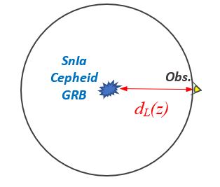
Figure 1: The luminosity distance is obtained from the apparent and absolute luminosities. Eq. (6) defines the quantity known as luminosity distance. It is straightforward to show that in an expanding flat Universe, where the energy is not conserved due to the increase of the photon wavelength and period with time, the luminosity distance can be expressed as (Dodelson, 2003; Perivolaropoulos, 2006)
(7) The luminosity distance is an important cosmological observable that is measured using standard candles (see Subsection II.1.1)
-
•
Angular diameter distance
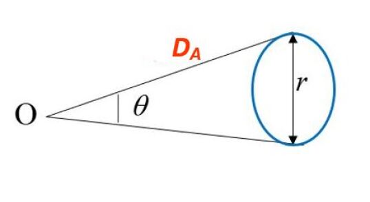
Figure 2: The angular diameter distance is obtained from the angular and physical scales. Consider a source (standard ruler) with a physical scale that subtends an angle in the sky (Fig. 2). In Euclidean space, assuming that is small, the physical angular diameter distance is defined as (e.g. Dodelson, 2003; Hobson et al., 2006)
(8) A particularly useful standard ruler is the sound horizon at recombination calibrated by the peaks of the CMB anisotropy spectrum and observed either directly through the CMB anisotropies or through its signatures in the large scale structure (Baryon Acoustic Oscillations (BAO)) (see Subsection II.1.2).
It is straightforward to show that in an expanding flat Universe the physical angular diameter distance can be expressed as (e.g. Dodelson, 2003)
(9)
The luminosity and angular diameter distances can be measured using standard candles and standard rulers thus probing the cosmic expansion rate at both the present time () and at higher redshifts ().
II.1.1 Standard candles as probes of luminosity distance
The luminosity distance to a source may be probed using standardizable candles like Type Ia supernovae (SnIa) () (Riess et al., 1998; Perlmutter et al., 1999; Betoule et al., 2014; Scolnic et al., 2018) and gamma-ray bursts (GRBs) () (Amati et al., 2008, 2019; Salvaterra et al., 2009; Tanvir et al., 2009; Samushia and Ratra, 2010; Schaefer, 2007; Cucchiara et al., 2011; Wang et al., 2016c; Demianski et al., 2017; Tang et al., 2019; Cardone et al., 2010; Khadka and Ratra, 2020a; Khadka et al., 2021; Dainotti et al., 2013; Dainotti and Del Vecchio, 2017; Dirirsa et al., 2019; Demianski et al., 2021; Cao et al., 2022b; Luongo et al., 2021; Cao et al., 2022a; Liu et al., 2022; Hu et al., 2021; Dai et al., 2021; Luongo and Muccino, 2021).
Surveys can indicate the distance-redshift relation of SnIa by measuring their peak luminosity that is tightly correlated with the shape of their characteristic light curves (luminosity as a function of time after the explosion) and the redshifts of host galaxies. The latest and largest SnIa dataset available that incorporates data from six different surveys is the Pantheon sample consisting of a total of SnIa in the redshift range (the number of SnIa with is only six) (Scolnic et al., 2018). More recently, the Pantheon+ sample which comprises 18 different samples has been released (Brout et al., 2022; Scolnic et al., 2021) (see also Peterson et al., 2021; Brownsberger et al., 2021). Brout et al. (2022); Scolnic et al. (2021) present 1701 light curves of distinct SnIa in the redshift range including SnIa which are in very nearby galaxies () with measured Cepheid distances. For determination of the SH0ES team (Riess et al., 2021b) use as calibrator sample SnIa in the Cepheid hosts and SnIa in the Hubble flow () from the Pantheon+ sample.
The apparent magnitude222The apparent magnitude of an astrophysical source detected with flux is defined as (10) where is a reference flux (zero point). The absolute magnitude of an astrophysical source is the apparent magnitude the source would have if it was placed at a distance of from the observer. of SnIa in the context of a specified form of , is related to their luminosity distance of Eq. (7) in Mpc as
| (11) |
Using now the dimensionless Hubble free luminosity distance
| (12) |
the apparent magnitude can be written as
| (13) |
The use of Eq. (13) to measure using the measured apparent magnitudes of SnIa requires knowledge of the value of the SnIa absolute magnitude which can be obtained using calibrators of local SnIa at (closer than the start of the Hubble flow) in the context of a distance ladder (e.g. Sandage et al., 2006) using calibrators like Cepheid stars.
In the cosmic distance ladder approach each step of the distance ladder uses parallax methods and/or the known intrinsic luminosity of a standard candle source to determine the absolute (intrinsic) luminosity of a more luminous standard candle residing in the same galaxy. Thus highly luminous standard candles are calibrated for the next step in order to reach out to high redshift luminosity distances.
II.1.1.1 SnIa standard candles and their calibration
-
•
SnIa-Cepheid: Geometric anchors may be used to calibrate the Cepheid variable star standard candles at the local Universe (primary distance indicators) whose luminosities are correlated with their periods of variability333The period–luminosity (PL) relation is also called the Leavitt law (Leavitt, 1908; Leavitt and Pickering, 1912).. The MW, the Large Magellanic Cloud (LMC) and NGC 4258 are used as distance geometric anchor galaxies. For Cepheids in the anchor galaxies there are three different ways of geometric distance calibration of their luminosities: trigonometric parallaxes in the MW (Benedict et al., 2007; van Leeuwen et al., 2007; Casertano et al., 2016; Riess et al., 2014; Lindegren et al., 2016; Riess et al., 2018b, a, 2021a), Detached Eclipsing Binary Stars (DEBs) in the LMC (Pietrzyński et al., 2019) and water masers (see Subsection II.1.5) in NGC 4258 (Yuan et al., 2022; Reid et al., 2019). The DEBs technique relies on surface-brightness relations and is a one-step distance determination to nearby galaxies independent from Cepheids (Pietrzyński et al., 2013).
Using the measured distances of the calibrated Cepheid stars the intrinsic luminosity of nearby SnIa residing in the same galaxies as the Cepheids is obtained. This SnIa calibration which fixes is then used for SnIa at distant galaxies to measure () and ().
-
•
SnIa-TRGB: Instead of Cepheid variable stars, the Tip of the Red Giant Branch (TRGB) stars in the Hertzsprung-Russell diagram (Beaton et al., 2016; Freedman et al., 2020) and Miras (Huang et al., 2018, 2019) (see also Czerny et al., 2018, for a review) can be used as calibrators of SnIa. The Red Giant stars have nearly exhausted the hydrogen in their cores and have just began helium burning (helium flash phase). Their brightness can be standardized using parallax methods and they can serve as bright standard candles visible in the local Universe for the subsequent calibration of SnIa.
-
•
SnIa-Miras: Miras (named for the prototype star Mira) are highly evolved low mass variable stars at the tip of asymptotic giant branch (AGB) stars (e.g. Iben and Renzini, 1983). The water megamaser as distance indicator (see Subsection II.1.5) can be used to calibrate the Mira period–luminosity (PL) relation (Huang et al., 2018). Miras with short period ( days) have low mass progenitors and are present in all galaxy types or in the halos of galaxies, eliminating the necessity for low inclination SnIa host galaxies.
-
•
SBF: Another method to determine the Hubble constant based on calibration of the peak absolute magnitude of SnIa is the Surface Brightness Fluctuations (SBF) method (Jensen et al., 2001; Cantiello et al., 2018; Khetan et al., 2021). SBF is a secondary444Nearby Cepheids or stellar population models are used for the empirical or theoretical calibration of the SBF distances respectively. luminosity distance indicator that uses stars in the old stellar populations (II) and can reach larger distances than Cepheids even inside the Hubble flow region where the recession velocity is larger than local peculiar velocities () (Tonry and Schneider, 1988; Tonry et al., 1997; Blakeslee et al., 1999; Mei et al., 2005; Biscardi et al., 2008; Blakeslee et al., 2009; Blakeslee, 2012). For SBF calibration Blakeslee et al. (2021) use both Cepheids and TRGB demonstrating that these calibrators are consistent with each other.
Assume that a galaxy includes a finite number of stars covering a range of luminosity. Using SBF in the galaxy image for the determination of its distance, the ratio of the second and first moments of the stellar luminosity function in the galaxy is used along with the mean flux per star as follows (Tonry and Schneider, 1988; Blakeslee et al., 1999)
(14) where
(15) where is the expectation number of stars with luminosity . Thus SBF can be viewed as providing an average brightness. A galaxy with double distance appears with double smoothness due to the effect of averaging.
II.1.1.2 Alternative cosmological standard candles
-
•
SneII: An independent method to determine the Hubble constant utilizes Type II supernovae (SneII) as cosmic distance indicators (de Jaeger et al., 2020a). SneII are characterised by the presence of hydrogen lines in their spectra (Filippenko, 1997, 2000). This feature distinguishes SneII from other types of supernovae. Their light curve shapes include a plateau of varying steepness and length differ significantly from those of SnIa. The use of SneII as standard candles is motivated by the fact that they are more abundant than SnIa (Li et al., 2011; Graur et al., 2017) (although - mag fainter Richardson et al., 2014) and are produced by different stellar populations than SnIa which are more difficult to standardize. The SneII progenitors (red super giant stars) however are better understood than those of SnIa.
Different SneII distance-measurement techniques have been proposed and tested. These include, the expanding photosphere method (Kirshner and Kwan, 1974; Eastman et al., 1996; Dessart and Hillier, 2005), the spectral-fitting expanding atmosphere method (Baron et al., 2004; Dessart et al., 2008), the standardized candle method (Hamuy and Pinto, 2002), the photospheric magnitude method (Rodríguez et al., 2014) and the photometric color method (de Jaeger et al., 2015). For example, the standardized candle method is based on the relation between the luminosity and the expansion velocity of the photosphere (Hamuy and Pinto, 2002; Olivares E. et al., 2010; de Jaeger et al., 2017, 2020b).
-
•
GRBs: In addition to SnIa and SneII, GRBs are widely proposed as standard candles to trace the Hubble diagram at high redshifts (Lamb and Reichart, 2000; Basilakos and Perivolaropoulos, 2008; Wang et al., 2015; Khadka and Ratra, 2020a; Khadka et al., 2021). However GRBs distance calibration is not easy and various cosmology independent methods (e.g. Liu and Wei, 2015) or phenomenological relations (e.g. Amati et al., 2002; Ghirlanda et al., 2004) have been proposed for their calibration.
II.1.1.3 Using SnIa to measure and :
The best fit values of the parameter and the deceleration parameter may be obtained555 is the deceleration parameter (Camarena and Marra, 2020b) using local distance ladder measurements (e.g. Cepheid calibration up to ) to measure directly , low measurements of the SnIa apparent magnitude and a kinematic local expansion of () as (e.g. Weinberg, 2008)
| (16) |
Alternatively, may be fixed to its CDM value and may be fit as a single parameter (Riess et al., 2011, 2016, 2019).
Using higher SnIa the best fit parameters of CDM may be obtained by fitting the CDM expansion rate
| (17) |
where is the matter density parameter today.
Using Eqs. (7), (12) and (17), the Hubble free luminosity distance can be written as
| (18) |
A key assumption in the use of SnIa in the measurement of and is that they are standardizable and after proper calibration they have a fixed absolute magnitude independent of redshift666The possibility for intrinsic luminosity evolution of SnIa with redshift was first pointed out by Tinsley (1968). Also, the assumption that the luminosity of SnIa is independent of host galaxy properties (e.g. host age, host morphology, host mass) and local star formation rate has been discussed in Kang et al. (2020); Rose et al. (2019); Jones et al. (2018); Rigault et al. (2020); Kim et al. (2018).. This assumption has been tested in Colgáin (2019); Kazantzidis and Perivolaropoulos (2019, 2020); Sapone et al. (2021); Koo et al. (2020); Kazantzidis et al. (2021); Luković et al. (2020); Tutusaus et al. (2019, 2017); Drell et al. (2000).
Using the degenerate combination
| (19) |
into Eq. (13) we obtain
| (20) |
The theoretical prediction (20) may now be used to compare with the observed data and to obtain the best fits for the parameters and . Using the maximum likelihood analysis the best fit values for these parameters may be found by minimizing the quantity
| (21) |
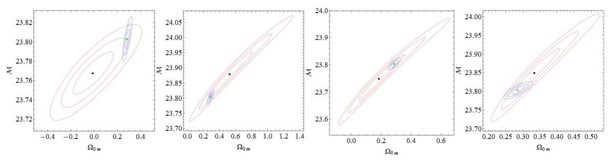
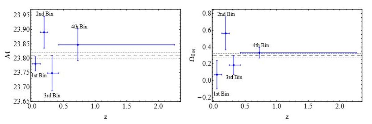
The results from the recent analysis by Kazantzidis and Perivolaropoulos (2020) using the latest SnIa (Pantheon) data (Scolnic et al., 2018) (consisting of 1048 datapoints in the redshift range sorting them from lowest to highest redshift and dividing them in four equal uncorrelated bins) in the context of a CDM model are shown in Figs. 3 and 4777For as indicated by Cepheid calibrators (Camarena and Marra, 2020b) of SnIa at and the SnIa local determination (Riess et al., 2019) Kazantzidis and Perivolaropoulos (2020) find which is consistent with the full Pantheon SnIa best fit shown in Fig. 3.. An oscillating signal for and () is apparent in Fig. 4 and its statistical significance may be quantified using simulated data (Kazantzidis et al., 2021; Koo et al., 2020).
The presence of large scale inhomogeneities at low including voids or a supercluster (Grande and Perivolaropoulos, 2011) can be a plausible physical explanation for this curious behavior. In the context of a local void model the analysis by Kazantzidis and Perivolaropoulos (2020) indicated that the value of increases by which is less than the required to address the Hubble tension. The bias and systematics induced by such inhomogeneities on the Hubble diagram within a well-posed fully relativistic framework (light cone averaging formalism Gasperini et al., 2011) has been discussed in Fanizza et al. (2020).
Marra and Perivolaropoulos (2021) have pointed out that this tension is related to the mismatch between the SnIa absolute magnitude calibrated by Cepheids at (Camarena and Marra, 2020b, 2021)
| (22) |
and the SnIa absolute magnitude using the parametric free inverse distance ladder calibrating SnIa absolute magnitude using the sound horizon scale (Camarena and Marra, 2020a)
| (23) |
Thus a transition in the absolute magnitude with amplitude may provide a solution to this tension (see Subsection II.2.4 and in Alestas et al., 2021b; Marra and Perivolaropoulos, 2021). Alternatively if this discrepancy is not due to systematics (Follin and Knox, 2018; Verde et al., 2019), it could be an indication of incorrect estimate of the sound horizon scale due e.g. to early dark energy (Chudaykin et al., 2020) or to late phantom dark energy (Alestas et al., 2020a).
Note also that Rameez and Sarkar (2021) find discrepancies between ’Joint Light-curve Analysis’ (JLA) SnIa and Pantheon SnIa datasets which imply an uncertainty in the calibration of the absolute magnitude or equivalently of the Hubble constant which is large enough to undermine the claim for Hubble tension.
II.1.1.4 Observational data - Constraints:
-
•
SnIa-Cepheid: Using the analysis of the Hubble Space Telescope (HST) observations (Sandage et al., 2006) the Hubble constant value has been measured from Cepheid-calibrated supernovae (using 70 long-period Cepheids in the LMC) by the Supernovae for the Equation of State (SH0ES) of dark energy collaboration (Riess et al., 2011, 2016, 2019). The analysis by the SH0ES Team using this local model-independent measurement refers (Riess et al., 2021b), which results in tension with the value estimated by CMB Planck18 (Aghanim et al., 2020e) assuming the CDM model while in previous analysis by SH0ES Team (Riess et al., 2021a) using the Gaia Early Data Release (EDR) parallaxes (Gaia Collaboration et al., 2020) and reaching precision by improving the calibration a value of is obtained, a tension with the prediction from Planck18 CMB observations. Riess et al. (2018b) analysing the HST data, using Cepheids as distance calibrators reports . A reanalysis of the SH0ES collaboration results using a cosmographic method allowing also the deceleration parameter to be a free parameter by Camarena and Marra (2021) leads to .
Breuval et al. (2020) considered companion and average cluster parallaxes instead of direct Cepheid parallaxes and obtained (ZP) when all Cepheids are considered and (ZP) for fundamental mode pulsators only (where ZP is the second Gaia data release (GDR2) (Brown et al., 2018) parallax zero point).
Various other previous estimates of have been obtained by treatments of the distance ladder (Dhawan et al., 2018; Burns et al., 2018; Feeney et al., 2018). In particular, Dhawan et al. (2018) find (statistical) (systematic) using SnIa as standard candles in the near-infrared (NIR), Burns et al. (2018) find analysing the final data release of the Carnegie Supernova Project888https://csp.obs.carnegiescience.edu (CSP) I (Krisciunas et al., 2017) and Feeney et al. (2018) find using a Bayesian hierarchical model of the local distance ladder.
-
•
SnIa-TRGB: The Carnegie–Chicago Hubble Program999https://carnegiescience.edu/projects/carnegie-hubble-program (CCHP) (Beaton et al., 2016) using calibration of SnIa with the TRGB method estimates (Freedman et al., 2019) and a revision of their measurements has lead to (Freedman et al., 2020). Recently, the updated TRGB calibration applied to a distant sample of SnIa from the CCHP lead to a value of the Hubble constant of (Freedman, 2021). Using the LMC and the NGC 4258 as TRGB calibration of the SnIa distance ladder, the SH0ES team finds (Yuan et al., 2019) and (Reid et al., 2019) respectively. Freedman (2021); Freedman et al. (2020); Hoyt (2021) argue that the difference in the derived value of by SH0ES team compared to CCHP was due to incorrect assumptions regarding calibration of the TRGB in the LMC made by Yuan et al. (2019). A value of is obtained by Kim et al. (2020) using peculiar velocities and TRGB distances of 33 galaxies located between the Local Group and the Virgo cluster () (mainly the sample of Virgo infall galaxies from Karachentsev et al., 2018).
More recently, Soltis et al. (2021) have reported a measurement of using the TRGB distance indicator calibrated from the European Space Agency (ESA) Gaia mission Early Data Release 3 (EDR3) trigonometric parallax of Omega Centauri (Gaia Collaboration et al., 2020). Anand et al. (2021) find combining TRGB measurements with either the Pantheon or CSP samples of supernova. Finally, Jones et al. (2022) using NIR only cosmological analysis and TRGB distances to calibrate the SnIa luminosity of the CSP and RAISIN (an anagram for “SnIa in the IR”) samples (Jones et al., 2017; Brout et al., 2019) and Dhawan et al. (2022) using TRGB calibration of SnIa observed by the Zwicky Transient Facility (ZTF) (Bellm et al., 2018; Graham et al., 2019) report and respectively.
-
•
SnIa-Miras: Calibration of SnIa in the host NGC 1559 galaxy with the Miras method using a sample of 115 oxygen-rich Miras101010Miras can be divided into oxygen- and carbon-rich Miras. discovered in maser host NGC 4258 galaxy, has lead to a measurement of the Hubble constant as (Huang et al., 2019).
-
•
SBF: Calibrating the SnIa luminosity with SBF method and extending it into the Hubble flow by using a sample of SnIa in the redshift range , extracted from the Combined Pantheon Sample has lead to the measurement (stat) (sys) by Khetan et al. (2021). Previously Cantiello et al. (2018) combining distance measurement with the corrected recession velocity of NGC reported a Hubble constant . A new measurement of the Hubble constant has recently been obtained based on a set of SBF (Blakeslee et al., 2021) distances extending out to .
-
•
SneII: SneII have also been used for the determination of . Using SneII as cosmological standardisable candles with host-galaxy distances measured from Cepheid variables or the TRGB the Hubble constant was measured to be (de Jaeger et al., 2020a). More recently, de Jaeger et al. (2022) find using 13 SneII.
II.1.2 Sound horizon as standard ruler: early time calibrators
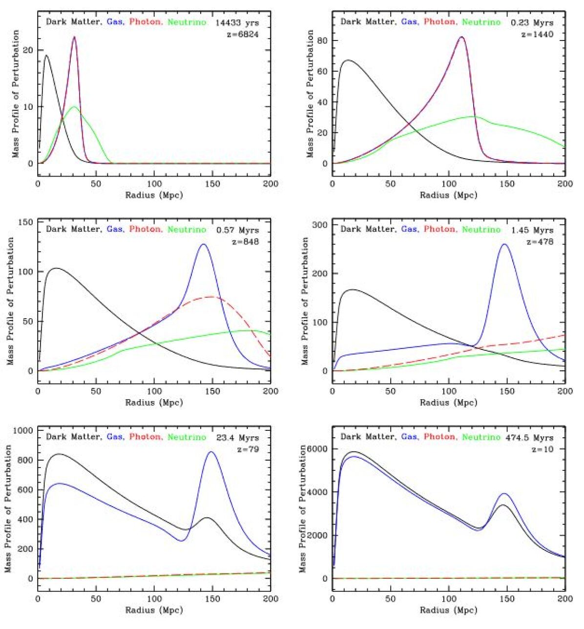
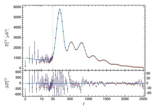
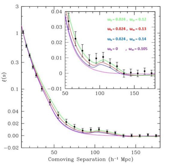
Before recombination (), the primeval plasma of coupled baryons to photons (baryon-photon fluid) oscillates as spherical sound waves emanating from baryon gas perturbations are driven by photon pressure. At recombination when the Universe has cooled enough the electrons and protons combine to form hydrogen (e.g. Peebles, 1968), photons decouple from baryons and propagate freely since the pressure becomes negligible. Thus the spherical sound wave shells of baryons become frozen. This process which was first detected in the galaxy power spectrum by Cole et al. (2005); Eisenstein et al. (2005) is illustrated in Fig. 5. It inflicts a unique Baryon Acoustic Oscillations (BAO) scale on the CMB anisotropy spectrum peaks shown in Fig. 6 and on the matter large scale structure (LSS) power spectrum on large scales at the radius of the sound horizon (the distance that the sound waves have traveled before recombination). This scale emerges as a peak in the correlation function 111111The correlation function is defined as the excess probability of one galaxy to be found within a given distance of another. Using the Landy-Szalay estimator (Landy and Szalay, 1993) this function can be computed (Eisenstein et al., 2005) (24) where is the comoving galaxy separation distance and , and correspond to the number of galaxy pairs with separations in real-real, random-random and real-random catalogs, respectively. as illustrated in Fig. 7 or equivalently as damped oscillations in the LSS power spectrum (Eisenstein and Hu, 1998; Eisenstein et al., 2005; Meiksin et al., 1999; Matsubara, 2004).
The characteristic BAO scale is also imprinted in the Lyman- (Ly) forest absorption lines of neutral hydrogen in the intergalactic medium (IGM) detected in quasar (QSO) spectra.
The measured angular scale of the sound horizon at the drag epoch when photon pressure vanishes can be used to probe the Hubble expansion rate using the standard ruler relation (e.g. Peebles, 1980; Amendola and Tsujikawa, 2015)
| (25) |
where is the comoving angular diameter distance to last scattering (at redshift ) and is the radius of sound horizon at last scattering.
The radius of the sound horizon at last scattering can be calculated by the distance that sound can travel from the Big Bang, , to time at the drag epoch when the photon pressure can no longer prevent gravitational instability in baryons. This happens shortly after the time of the last scattering when the optical depth due to Thomson scattering reaches unity (Eisenstein and Hu, 1998). Thus (Aubourg et al., 2015)
| (26) |
where the drag redshift corresponds to time , , and denote the densities for baryon, cold dark matter and radiation (photons) respectively and is the sound speed in the photon-baryon fluid given by (Efstathiou and Bond, 1999; Komatsu et al., 2009)
| (27) |
The expansion rate depends on the ratio of the matter density to radiation density and the sound speed determined by the baryon-to-photon ratio. Both the matter-to-radiation ratio and the baryon-to-photon ratio can be estimated from the details of the acoustic peaks in CMB anisotropy power spectrum (e.g. Hu and Dodelson, 2002). Thus the CMB is possible to lead to an independent determination of the radius of sound horizon. Alternatively an independent determination of the radius of sound horizon can obtained using primordial deuterium measurements (Addison et al., 2013, 2018). Now using the Eqs. (9) and (25) we can write the angular size of the sound horizon as
| (28) |
where is the dimensionless normalized Hubble parameter and for a flat CDM model is given by
| (29) |
Eq. (28) indicates that there is a degeneracy between , and . Thus can not be derived using the BAO data alone which constrain and the degeneracy is broken when is fixed using either CMB power spectra (Zarrouk et al., 2018) or deuterium abundance (Addison et al., 2013, 2018).
For example is inferred from Planck18 TT,TE,EE+lowE CMB data (Aghanim et al., 2020e). Using the independent determination of , measuring the angular acoustic scale from the location of the first acoustic peak in the CMB spectrum and fitting the integral in Eq. (28) using low z BAO or SnIa data, the Hubble constant can be derived. This is the ’inverse distance ladder’ approach (Aubourg et al., 2015; Cuesta et al., 2015; Cai et al., 2022a) which uses the sound horizon scale calibrated by the CMB peaks or by Big Bang Nucleosynthesis (BBN) (Schöneberg et al., 2019) instead of the SnIa absolute magnitude calibrated by Cepheid stars to obtain .
The deformation of the expansion rate before recombination using additional components like early dark energy that increase in Eq. (26) and thus decrease and increase the predicted value of for fixed measured in Eq. (28), has been used as a possible approach to the solution of the Hubble tension. A challenge for this class of models is the required fine-tuning so that the evolution of returns quickly to its standard form after recombination for consistency with lower cosmological probes and growth measurements (Pogosian et al., 2010). The assumed increase of at early times has been claimed to lead to a worsened growth tension (Jedamzik et al., 2021) as discussed below even though the issue is under debate (Smith et al., 2021; Chudaykin et al., 2021).
II.1.2.1 Observational data - Constraints
-
•
CMB: The measurement of the Hubble constant using the sound horizon at recombination as standard ruler calibrated by the CMB anisotropy spectrum is model dependent and is based on assumptions about the nature of dark matter and dark energy as well as on an uncertain list of relativistic particles (see Chang et al., 2022b, for a review). The best fit value obtained by the Planck18/CDM CMB temperature, polarization, and lensing power spectra is (Aghanim et al., 2020e). The measurements of the CMB from the combination Atacama Cosmology Telescope (ACT)121212https://act.princeton.edu and Wilkinson Microwave Anisotropy Probe (WMAP) estimated the Hubble constant to be and from ACT alone to be (Aiola et al., 2020). Note that the analysis of the nine-year data release of WMAP (Hinshaw et al., 2013) alone prefers a value for the Hubble constant . More recently, Balkenhol et al. (2021) obtain CMB-based constraints on Hubble parameter using combined South Pole Telescope131313https://pole.uchicago.edu (SPT), Planck, and ACT DR4 datasets. Dutcher et al. (2021) find using SPT-3G data alone, while a previous analysis of SPT data by Henning et al. (2018) results in .
-
•
BAO: The analysis of the wiggle patterns of BAO is an independent way of measuring cosmic distance using the CMB sound horizon as a standard ruler. This measurement has improved in accuracy through a number of galaxy surveys which detect this cosmic distance scale: the Sloan Digital Sky Survey (SDSS) supernova survey (York et al., 2000; Tegmark et al., 2006) encompassing the Baryon Oscillation Spectroscopic Survey (BOSS) which has completed three different phases (Dawson et al., 2013). Its fourth phase (SDSS-IV) (Blanton et al., 2017) encompasses the Extended Baryon Oscillation Spectroscopic Survey (eBOSS) (Dawson et al., 2016) (see also Alam et al., 2021a; Gil-Marin et al., 2020; Neveux et al., 2020; Raichoor et al., 2020; Hou et al., 2020), the WiggleZ Dark Energy Survey (Drinkwater et al., 2010; Blake et al., 2011a, 2012), the -degree Field Galaxy Redshift Survey (dFGRS) (Colless et al., 2001; Cole et al., 2005), the -degree Field Galaxy Survey (dFGS) (Jones et al., 2009; Beutler et al., 2011, 2012).
More recently, BAO measurements have been extended in the context of quasar redshift surveys and Ly absorption lines of neutral hydrogen in the IGM detected in QSO spectra using the complete eBOSS survey. The measurement of BAO scale using first the auto-correlation of Ly function (Delubac et al., 2015; de Sainte Agathe et al., 2019; Bautista et al., 2017) and then the Ly-quasar cross-correlation function (Font-Ribera et al., 2014; Blomqvist et al., 2019) or both the auto- and cross-correlation functions (du Mas des Bourboux et al., 2020) pushed BAO measurements to higher redshifts (). Recent studies present BAO measurements from the Ly using the eBOSS sixteenth data release (DR) (Ahumada et al., 2020) of the SDSS IV (e.g. du Mas des Bourboux et al., 2020).
As discussed in subsection II.1.2 BAO data alone cannot constrain because BAO observations measure the combination rather than and individually (where is the radius of sound horizon). Using the CMB calibrated physical scale of the sound horizon and the combination of BAO with SnIa data (i.e inverse distance ladder) the value was reported which is in agreement with the value obtained by CMB data alone (Aubourg et al., 2015). The analysis by Wang et al. (2017) using a combination of BAO measurements from 6dFGS (Beutler et al., 2011), Main Galaxy Sample (MGS) (Ross et al., 2015), BOSS DR12 and eBOSS DR14 quasar sample in a flat CDM cosmology reports . Using BAO measurements and CMB data from WMAP, Zhang and Huang (2019) reported the constraints of . The analysis by Addison et al. (2018) combining galaxy and Ly forest BAO with a precise estimate of the primordial deuterium abundance (BBN) results in for the flat CDM model. Alam et al. (2021b) find using BOSS galaxy and eBOSS, with the BBN prior independent from the CMB anisotropies. D’Amico et al. (2020) obtain performing a analysis for the cosmological parameters of the DR12 BOSS data using the Effective Field Theory of Large-Scale Structure (EFTofLSS) formalism141414The EFTofLSS formalism can provide a prediction of the LSS clustering in the mildly non-linear regime (D’Amico et al., 2021a; Baumann et al., 2012; Carrasco et al., 2012; Porto et al., 2014; Perko et al., 2016). and Colas et al. (2020) obtain assuming a BBN prior on the baryon fraction of the energy density instead of the baryon/dark-matter ratio.
Recently, Pogosian et al. (2020) report the constraints of using BAO data, including the released eBOSS DR16, and CMB data from Plank. Zhang et al. (2022) infer imposing BBN priors on the baryon density and combining the BOSS Full Shape with the BAO measurements from BOSS and eBOSS. Also, a new analysis of galaxy 2-point functions in the BOSS survey, including full-shape information and post-reconstruction BAO by Chen et al. (2022) results in and a full-shape analysis of BOSS DR12 by Philcox and Ivanov (2022) results in . A previous analysis of BOSS DR12 on anisotropic galaxy clustering in Fourier space by Ivanov et al. (2020c) gives . Finally, analyzing the BOSS DR12 galaxy power spectra using a new approach based on the horizon scale at matter-radiation equality Farren et al. (2021) find and adding Planck lensing Philcox et al. (2021) find .
II.1.3 Time delays: gravitational lensing
Gravitational lensing time-delay cosmography can be used to measure . This approach was first proposed by Refsdal (1964) and recently implemented by Shajib et al. (2020); Wong et al. (2020); Birrer et al. (2020) (see also Treu and Marshall, 2016; Suyu et al., 2018, for clear reviews).
Strong gravitational lensing (Refsdal, 1964) arises from the gravitational deflection of light rays of a background source when an intervening lensing mass distribution (e.g. a massive galaxy or cluster of galaxies) exists along the line of sight. The light rays go through different paths such that multiple images of the background source appear around the intervening lens (Oguri, 2019).
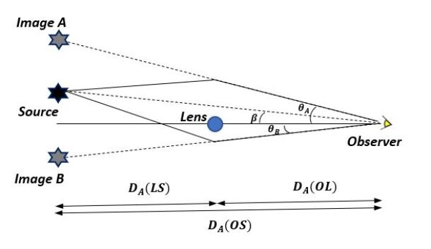
The time delay between two images and by a single deflector originating from the same source at angle shown in Fig. 8 is given as (Suyu et al., 2010)
| (30) |
where is the lens redshift, is the angular diameter distance to the lens, is the angular diameter distance to the source, is the angular diameter distance between the lens and the source and is the Fermat potential (e.g. Suyu et al., 2010)
| (31) |
with the lensing potential at the image direction. The time delay in Eq. (30) is thus connected to the time delay distance defined as (e.g. Suyu et al., 2010, 2017)
| (32) |
This distance is inversely proportional to
| (33) |
and thus its measurement constrains . Strongly lensed quasars (bright and time variable sources) lensed by a foreground lensing mass are used to measure the above observable time delay on cosmologically interesting scales (Keeton and Kochanek, 1997; Kochanek, 2003; Oguri, 2007; Bonvin et al., 2017; Wong et al., 2020). Active galactic nuclei (AGN) constitute another background source which may be used to measure the time delay (Kochanek et al., 2006; Fassnacht et al., 1999; Eigenbrod et al., 2006). Recently, Qi et al. (2022) proposed the strongly lensed SnIa as a precise late-universe probe to improve the measurements on the Hubble constant and cosmic curvature. The inference of from is relatively insensitive to the assumed background cosmology.
Note that a source of systematic effects in time delay cosmography is the uncertainty of the mass along the line of sight modeling with respect to the mass sheet transformation (MST). This is a mathematical degeneracy (e.g. Falco et al., 1985; Gorenstein et al., 1988; Saha and Williams, 2006; Schneider and Sluse, 2014; Kochanek, 2002, 2020) and can bias the strong lensing determination of Hubble constant (Kochanek, 2021).
II.1.3.1 Observational data - Constraints:
Strong gravitational lensing time delay measurements of are consistent with the local measurements using late time calibrators and in mild tension with Planck (e.g. Bonvin et al., 2017). The method of the measurement of Lenses in COSMOGRAIL’s Wellspring (HLiCOW) collaboration (Wong et al., 2020) is independent of the cosmic distance ladder and is based on time delays between multiple images of the same source, as occurs in strong gravitational lensing.
Using joint analysis of six gravitationally lensed quasars with measured time delays from the COSmological MOnitoring of GRAvItational Lenses (COSMOGRAIL) project, the value was obtained which is in tension with Planck CMB. Assuming the Universe is flat and using lensing systems from the lensing program HLiCOW and the Pantheon supernova compilation a value of was reported by the analysis of Ref. (Liao et al., 2019). A similar value of was found using updated HLiCOW dataset consisting of six lenses (Liao et al., 2020). The reanalysis of the four publicly released lenses distance posteriors from the H0LiCOW by Yang et al. (2020b) leads to . The analysis of the strong lens system DES by Shajib et al. (2020) for strong lensing insights into dark energy survey collaboration (STRIDES), infers in the CDM cosmology. The analysis by Birrer et al. (2020) based on the strong lensing and using Time-Delay COSMOgraphy (TDCOSMO151515TDCOSMO collaboration (Millon et al., 2020) was formed by members of H0LiCOW, STRIDES, COSMOGRAIL and SHARP., 161616http://www.tdcosmo.org/) data set alone infers and using a joint hierarchical analysis of the TDCOSMO and Sloan Lens ACS (SLACS) (Bolton et al., 2006) sample reports . Chen et al. (2019) based on a joint analysis of 3 strong lensing system, using ground-based adaptive optics (AO) from SHARP AO effort and the HST find . A reanalysis of six of the TDCOSMO lenses using a power-law mass profile model results in (Millon et al., 2020). Analysing strongly, quadruply lensing systems Denzel et al. (2021) present a determination of the Hubble constant which is consistent with both early and late Universe observations. The value was reported by Qi et al. (2021) by combining the observations of ultra-compact structure in radio quasars and strong gravitational lensing with quasars acting as background source.
II.1.4 Standard sirens: gravitational waves
An independent and potentially highly effective approach for the measurement of and the Hubble constant is the use of gravitational wave (GW) observations and in particular those GW bursts that have an electromagnetic counterpart (standard sirens) (Schutz, 1986; Holz and Hughes, 2005; Dalal et al., 2006; Nissanke et al., 2010, 2013). In analogy with the traditional standard candles, it is possible to use standard sirens to directly measure the luminosity distance of the GW source.
Standard sirens involve the combination of a GW signal and its independently observed electromagnetic (EM) counterpart. Such counterpart may involve short gamma-ray bursts (SGRBs) signal from binary neutron star mergers (Eichler et al., 1989) or associated isotropic kilonova emission (Coulter et al., 2017; Soares-Santos et al., 2017) and enables the immediate identification of the host galaxy. In contrast to traditional standard candles such as SnIa calibrated by Cepheid variables, standard sirens do not require any form of cosmological distance ladder. Instead they are calibrated in the context of general relativity through the observed GW waveform.
The simultaneous observations of the GW signal and its EM counterpart (multi-messenger observations) of nearby compact-object merger leads to a measurement of the luminosity distance which depends on the inclination angle of the binary orbit with respect to the line of sight and the redshift (measured using photons) of the host galaxy respectively. An EM counterpart detected with a GW observation can further constrain the inclination angle and may also indicate the source’s sky position and the GW merger’s time and phase (e.g. Nissanke et al., 2013).
In the case of GW events with small enough localization volumes without an observed EM counterpart (dark sirens) (Chen et al., 2018) a statistical analysis over a set of potential host galaxies within the event localization region may provide redshift information. A candidate for such statistical method is a merger of stellar-mass binary black holes171717The stability analysis of the structures around black holes have been widely employed in the literature (see e.g. Kiuchi et al., 2011; Belczynski et al., 2016; Cunha et al., 2017; Aretakis, 2011; Alestas et al., 2020b). (BBH) which is usually not expected to result in bright EM counterparts unless it takes place in significantly gaseous environment (Graham et al., 2020). For example, GW190521 (Abbott et al., 2020c) is a possible candidate with EM counterpart corresponding to a stellar-origin BBH merger in active galactic nucleus (AGN) disks (McKernan et al., 2019) detected by ZTF (Bellm et al., 2018; Graham et al., 2019).
Alternatively, in the absence of an EM counterpart the redshift can be determined by exploiting information on the properties of the source (e.g. the knowledge of neutron star equation of state) to derive frequency-dependent features in the waveform (Messenger and Read, 2012) or using the gravitational waveform to determine the redshift of the mass distribution of the sources (Taylor and Gair, 2012; Farr et al., 2019). Also, Leandro et al. (2022) use an alternative method, presented in Ding et al. (2019), for redshift determination by the statistical knowledge of the redshift distribution of sources. Trott and Huterer (2021) argue that any absolute determination of may be biased due to the fundamental degeneracy between redshift and and therefore can not lead to reliable determination of . According to Trott and Huterer (2021) the reliable determination of with GW can only be achieved using standard sirens.
The luminosity distance-redshift relation Eq. (7) determines the Universe’s expansion history and the associated cosmological parameters including the Hubble constant (Abbott et al., 2017a; Fishbach et al., 2019). In particular using the mergers of binary neutron stars (BNS), or a binary of a neutron star with a stellar-mass black hole (NS-BH), which are excellent standard sirens, both the luminosity distance (from the gravitational wave waveform) and redshift of the host galaxy (from the electromagnetic counterpart) can be measured.
Using a BNS or a NS-BH merger, the distance to the source can be estimated from the detected amplitude (r.m.s. - averaged over detector and source orientations) of the GW signal by the expression (Schutz, 1986; Andersson and Kokkotas, 1996; Jaranowski et al., 1996; Kokkotas and Stergioulas, 2005; Kokkotas, 2008)
| (34) |
where is the gravitational wave frequency, is the timescale of frequency change, is a known numerical constant. Assuming a flat181818In an open (closed) Universe the distance in Hubble’s law is given () Universe the luminosity distance can then be obtained from the relation
| (35) |
For nearby sources, the recession velocity using the Hubble’s law is determined by the expression
| (36) |
and using Eqs. (7), (12) and (35) is given by
| (37) |
At low redshifts using the local expansion Eq. (16) we obtain
| (38) |
which is approximated for (or ) as
| (39) |
Using Eqs. (36) and (38), the equation for the determination of as a function of observables, and is (e.g. Zhang et al., 2017)
| (40) |
where the deceleration parameter may be set by a fit to the GW data or may be fixed to its Planck/CDM best fit form ().
II.1.4.1 Observational data - Constraints:
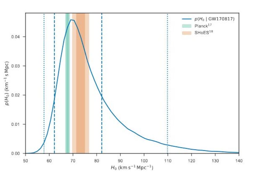
The first multi-messenger detection of a BNS merger, GW170817, by LIGO (Aasi et al., 2015) and Virgo (Acernese et al., 2015) interferometers enabled the first standard siren measurement of the Hubble constant . Using the BNS merger GW170817, the distance to the source was estimated to be (i.e. at redshift ) from the detected amplitude (r.m.s. - averaged over detector and source orientations) of the GW signal by the Eq. (34) (Abbott et al., 2017a). Also using the Hubble flow velocity inferred from measurement of the redshift of the host galaxy, NGC 4993 (NGC 4993 was identified as the unique host galaxy), the Hubble constant was determined to be (Abbott et al., 2017a) (see Fig. 9) by using Eq. (39).
Using continued monitoring of the the radio counterpart of GW17081 combining with earlier GW and EM data Hotokezaka et al. (2019) obtain a improved measurement of . Note that using the BNS merger GW170817 in Fishbach et al. (2019) and a statistical analysis (as first proposed in Schutz (1986)) over a catalog of potential host galaxies, the Hubble constant was determined to be . Using density-estimation Likelihood-Free Inference (LFI) Gerardi et al. (2021) focused on the inference of the cosmological expansion from GW-selected catalogues of BNS mergers with EM counterparts.
Also using the BBH merger GW170814 as a standard (dark) siren in the absence of an electromagnetic counterpart, combined with a photometric redshift catalog from the Dark Energy Survey (DES) (Abbott et al., 2018c) the analysis by Soares-Santos et al. (2019) results in . Using multiple GW observations (the BNS event GW170817 and the BBH events observed by advanced LIGO and Virgo in their first and second observing runs) in Abbott et al. (2021a) the Hubble constant was constrained as . Using the event GW190814 from merger of a black hole with a lighter compact object the Hubble constant was measured to be (Abbott et al., 2020a). In Mukherjee et al. (2020) the BBH merger GW190521 was analysed choosing the NRSur7dq4 waveform191919NRSur7dq4 is a numerical relativity surrogate 7-dimensional approximate waveform model of binary black hole merger with mass ratios (Varma et al., 2019). This model is made publicly available through the gwsurrogate (see https://pypi.org/project/gwsurrogate) and surfinBH (see https://pypi.org/project/surfinBH) Python packages. for the estimation of luminosity distance, after marginalizing over matter density when the CDM model is considered and using its EM counterpart ZTF19abanrhr202020The ZTF19abanrhr event was reported by ZTF (Bellm et al., 2018). This candidate EM counterpart is flare after a kicked BBH merger in the accretion disk of an AGN (McKernan et al., 2019) with peak luminosity occurred days after the BBH event GW19052. The ZTF19abanrhr was first observed after days from the GW detection at the sky direction (, ) and was associated with an AGN J124942.3 + 344929 at redshift (Graham et al., 2020). as identified in Graham et al. (2020) the Hubble constant was measured to be . The same study (Mukherjee et al., 2020) choosing different types of waveform finds and . Combining their results with the binary neutron star event GW170817 leads to . In Chen et al. (2020) for the same GW-EM event, assuming a flat wCDM model has obtained .
The analysis by Abbott et al. (2021b) using 47 gravitational-wave sources from the Third LIGO–Virgo–KAGRA Gravitational-Wave Transient Catalog (GWTC–3), infers . Palmese et al. (2021) find using the best available gravitational wave events, uniform galaxy catalog from the Dark Energy Spectroscopic Instrument (DESI) (Aghamousa et al., 2016a, b) Legacy Survey and combining with the GW170817. The value for GW190521 event was reported, and was obtained when combing the GW190521 with the results of the neutron star merger GW170817 (Gayathri et al., 2021). More recently, Mukherjee et al. (2022) report combining the bright standard siren measurement from GW170817 with a better measurement of peculiar velocity.
II.1.5 Megamaser technique
Observations of water megamasers which are found in the accretion disks around supermassive black holes (SMBHs) in active galactic nuclei (AGN) have been demonstrated to be powerful one-step geometric probes for measuring extragalactic distances (Herrnstein et al., 1999; Humphreys et al., 2013; Reid et al., 2013).
Assuming a Keplerian circular orbit around the SMBH, the centripetal acceleration and the velocity of a masing cloud are given as (Reid et al., 2013)
| (41) |
| (42) |
where is the Newton’s constant, is the mass of the central supermassive black hole, and is the distance of a masing cloud from the supermassive black hole.
The angular scale subtended by is given by
| (43) |
where is the distance to the galaxy.
Thus, from the velocity and acceleration measurements obtained from the maser spectrum, the distance to the maser may be determined
| (44) |
where is measured from the change in Doppler velocity with time by monitoring the maser spectrum on month timescales. Using Hubble’s law the Hubble constant may be approximated as (Reid et al., 2013)
| (45) |
where is the measured recessional velocity.
In order to constrain the Hubble constant the Megamaser Cosmology Project (MCP) (Reid et al., 2009) uses angular diameter distance measurements to disk megamaser-hosting galaxies well into the Hubble flow (). These distances are independent of standard candle distances and their measurements do not rely on distance ladders, gravitational lenses or the CMB (Pesce et al., 2020). Early measurements of using masers tended to favor lower values of while more recent measurements favor higher values as shown e.g. in Table LABEL:hubblevalue.
II.1.5.1 Observational data - Constraints:
Recently, the Megamaser Cosmology Project (MCP) (Reid et al., 2009) using geometric distance measurements to megamaser-hosting galaxies and assuming a global velocity uncertainty of associated with peculiar motions of the maser galaxies constrains the Hubble constant to be (Pesce et al., 2020). Previously the MCP reported results on galaxies, UGC with (Reid et al., 2013), NGC with (Kuo et al., 2013), NGC with (Kuo et al., 2015) and NGC with (Gao et al., 2016). Reid et al. (2019) use a improved distance estimation of the maser galaxy NGC (also known as Messier ) to calibrate the Cepheid-SN Ia distance ladder combined with geometric distances from MW parallaxes and DEBs in the LMC. The measured value of the Hubble constant is .
II.1.6 Tully-Fisher relation (TFR) as distance indicator
The Tully-Fisher (TF) method is a historically useful distance indicator based on the empirical relation between the intrinsic total luminosity (or the stellar mass) of a spiral galaxy212121Similarly, in the case of a elliptical galaxy the Faber–Jackson (FJ) empirical power-law relation (where is the luminosity of galaxy, the velocity dispersion of its stars and is a index close to ) (Faber and Jackson, 1976) can be used as a distance indicator. The FJ relation is the projection of the fundamental plane (FP) of elliptical galaxies which defined as (where is the effective radius and is the mean surface brightness within ) (Djorgovski and Davis, 1987). and its rotation velocity (or neutral hydrogen (HI) emission line width) (Tully and Fisher, 1977). This method has been used widely in measuring extragalactic distances (e.g. Sakai et al., 2000).
The Baryonic Tully Fisher relation (BTFR) (McGaugh et al., 2000; Verheijen, 2001; Gurovich et al., 2004; McGaugh, 2005) connects the rotation speed and total baryonic mass (stars plus gas) of a spiral galaxy as
| (46) |
where (with McGaugh et al., 2000; McGaugh, 2005; Lelli et al., 2016b) is a parameter and is the zero point in a log-log BTFR plot. This relation has been measured for hundreds of galaxies. The rotation speed can be measured independently of distance while the total baryonic mass may be used as distance indicator since it is connected to the intrinsic luminosity. Thus, the BTFR is a useful cosmic distance indicator approximately independent of redshift and thus can be used to obtain .
The BTFR has a smaller amount of scatter with a corresponding better accuracy as a distance indicator than the classic TF relation (Lelli et al., 2016b). In addition the BTFR recovers two decades in velocity and six decades in mass (McGaugh et al., 2000; McGaugh, 2005, 2012; Iorio et al., 2016; Lelli et al., 2019; Schombert et al., 2020).
A simple heuristic analytical derivation for the BTFR is obtained (Aaronson et al., 1979) by considering a star rotating with velocity in a circular orbit of radius around a central mass . Then the star velocity is connected with the central mass as
| (47) |
where is Newton’s constant and the surface density which may be shown to be approximately constant (Freeman, 1970). From Eqs. (46) and (47) we have
| (48) |
which indicates that the zero point intercept of the BTFR can probe both galaxy formation dynamics (through e.g. ) and possible fundamental constant dynamics (through ) (Alestas et al., 2021a).
II.1.6.1 Observational data - Constraints:
The analysis by Kourkchi et al. (2020) using infrared (IR) data of sample galaxies and the Tully Fisher relation determined the value of Hubble constant to be . In Schombert et al. (2020) a value of was found using Baryonic Tully Fisher relation for independent Spitzer photometry and accurate rotation curves (SPARC) galaxies222222The SPARC catalogue contains nearby (up to distances of ) late-type galaxies (spirals and irregulars) (Lelli et al., 2016a, b). The SPARC data are publicly available at http://astroweb.cwru.edu/SPARC. (up to distances of ).
II.1.7 Extragalactic background light -ray attenuation
This method is based on the fact that the extragalactic background light (EBL) which is a diffuse radiation field that fills the Universe from ultraviolet (UV) through infrared wavelength induces opacity for very high energy (VHE) photons () induced by photon-photon interaction (Hauser and Dwek, 2001). In this process a -ray and an EBL photon in the intergalactic medium may annihilate and produce an electron-positron pair (Gould and Schréder, 1966). The induced attenuation in the spectra of -ray sources is characterized by an optical depth that scales as (where is the photon density of the EBL, is the Thomson cross section, and is the distance from the -ray source to Earth). The cosmic evolution and the matter content of the Universe determine the -ray optical depth and the amount of -ray attenuation along the line of sight (Domínguez et al., 2019; Zeng and Yan, 2019). Thus a derivation of can be obtained by measuring the -ray optical depth with the -ray telescopes (Domínguez and Prada, 2013). This derivation is independent and complementary to that based on the distance ladder and cosmic microwave background (CMB) and seems to favor lower values of as shown in Table LABEL:hubblevalue.
II.1.7.1 Observational data - Constraints:
II.1.8 Cosmic chronometers
Cosmic chronometers are objects whose evolution history is known. For instance such objects are some types of galaxies. The observation of these objects at different redshifts and the corresponding differences in their evolutionary state has been used to obtain the value of at each redshift .
The cosmic chronometer technique for the determination of was originally suggested in Jimenez and Loeb (2002) and is based on the quasi-local () measurements along the Hubble flow of the Hubble parameter expressed as
| (49) |
Thus, the expansion rate may be obtained by measuring the age difference between two old and passively evolving galaxies232323These galaxies form only a few new stars and become fainter and redder with time. The time that has elapsed since they stopped star formation can be deduced. which are separated by a small redshif interval , to infer the (Moresco et al., 2012, 2016).
This approach determines the independent of the early-Universe physics and is not based on the distance ladder (e.g. Jimenez and Loeb, 2002; Chen et al., 2017; Farooq et al., 2017; Yu et al., 2018; Gómez-Valent and Amendola, 2018). The estimated values are more consistent with the values estimated from recent CMB and BAO data than those values estimated from SnIa. The value of can not be derived using the cosmic chronometers observations alone because there is a background degeneracy between and and this degeneracy is broken when these observations are combined.
II.1.8.1 Observational data - Constraints:
In Chen et al. (2017) the value of Hubble constant was found to be in the flat CDM model relying on measurements and their extrapolation to redshift zero. Analysing data determined by the cosmic chronometric (CCH) method, and data by BAO observations and using the Gaussian Process (GP) method (Seikel et al., 2012; Shafieloo et al., 2012; Yahya et al., 2014; Joudaki et al., 2018a) to determine a continuous function the Hubble constant is estimated to be by Yu et al. (2018). Also using the GP an extension of this analysis by Gómez-Valent and Amendola (2018), including the measurements obtained from Pantheon compilation and HST CANDELS and CLASH Multi-Cycle Treasury (MCT) programs, finds which is more consistent again with the lower range of values for . The GP method (Rasmussen and Williams, 2005) is used as a ’non-parametric’ technique which does not assume any parametrization or any cosmological model (see Ó Colgáin and Sheikh-Jabbari, 2021, for a discussion about GP as model independent method). The GP modeling approach has been performed by several authors to reconstruct cosmological parameters and thus to extract cosmological information directly from data (see e.g Benisty et al., 2022b; Escamilla-Rivera et al., 2021; Ren et al., 2022; Holsclaw et al., 2010b; Keeley et al., 2020b; Holsclaw et al., 2010a; Bengaly, 2022; Zhang and Xia, 2016; Busti et al., 2014; Seikel and Clarkson, 2013; Sahni et al., 2014; L’Huillier and Shafieloo, 2017; L’Huillier et al., 2018; Marques et al., 2019; Renzi and Silvestri, 2020; Benisty, 2021; Bonilla et al., 2021b, a; Sun et al., 2021; Escamilla-Rivera et al., 2021; Dhawan et al., 2021; Mukherjee and Banerjee, 2021; Keeley et al., 2021; Avila et al., 2021; Ruiz-Zapatero et al., 2022; Sharma et al., 2022; Renzi et al., 2021; Nunes et al., 2020; L’Huillier et al., 2020; Belgacem et al., 2020b; Pinho et al., 2018; Cai et al., 2017b; Haridasu et al., 2018; Zhang and Li, 2018; Wang and Meng, 2017b; Shafieloo et al., 2018; Bengaly et al., 2020a; Bengaly, 2020; Briffa et al., 2020; Li et al., 2021a).
Recently, a analysis by Moresco et al. (2022) reports and for a generic open wCDM and for a flat CDM respectively. The analysis by Moresco et al. (2022) examine the possible effects that can systematically bias the measurement and can affect the CC method. It should be pointed out however that the quality and reliability of cosmic chronometer data has been challenged by some authors. This is partly due to the fact that these datapoints are not model independent and are obtained by combining several datasets (Gómez-Valent and Amendola, 2018). This has improved significantly in the context of the aforementioned analysis by Moresco et al. (2022) where a detailed study of the covariance matrix and the effects of systematics has been implemented.
II.1.9 HII galaxy measurements
The ionized hydrogen gas (HII) galaxies (HIIG) emit massive and compact bursts generated by the violent star formation (VSF) in dwarf irregular galaxies. The HIIG measurements can be used to probe the background evolution of the Universe. This method of determination is based on the standard candle calibration provided by a (luminosity-velocity dispersion) relation. This relation exists in HIIGs and Giant extragalactic HII regions (GEHR) in nearby spiral and irregular galaxies. The turbulent emission line ionized gas velocity dispersion of the prominent Balmer lines242424The Balmer series, or Balmer lines is one of a set of six named series describing the spectral line emissions of the hydrogen atom. This is characterized by the electron transitioning from to (where n is the principal quantum number of the electron. The transitions to and to are called H-alpha and H-beta respectively. H-alpha () and H-beta () relates with its integrated emission line luminosity (Melnick et al., 2000; Siegel et al., 2005; Plionis et al., 2011; Chávez et al., 2012, 2014; Terlevich et al., 2015; Wei et al., 2016; Chávez et al., 2016; Yennapureddy and Melia, 2017; González-Morán et al., 2019). The relationship between and has a small enough scatter to define a cosmic distance indicator (that can be utilized out to ) independently of redshift and can be approximated as (Chávez et al., 2012, 2014; Terlevich et al., 2015; Wei et al., 2016; Leaf and Melia, 2018; Chávez et al., 2016; Yennapureddy and Melia, 2017; Ruan et al., 2019a; González-Morán et al., 2019)
| (50) |
where and are constants representing the slope and the logarithmic luminosity at .
From Eq. (6) the luminosity is given by
| (51) |
Thus using Eq. (50), the distance modulus of an HIIG can be obtained (Wei et al., 2016; Leaf and Melia, 2018; Chávez et al., 2016; Yennapureddy and Melia, 2017; Ruan et al., 2019a; González-Morán et al., 2019)
| (52) |
This observational distance modulus can be compared with the theoretical distance modulus. From the Eq. (11) this is given
| (53) |
Using now the dimensionless Hubble free luminosity distance Eq. (12) this can be written as
| (54) |
In order to obtain the best fit values for the parameters and this theoretical prediction may now be used to compared with the observed data. Using the maximum likelihood analysis the best fit values for these parameters may be found in the usual manner by minimizing the quantity
| (55) |
where is the uncertainty of the measurement.
II.1.9.1 Observational data - Constraints:
Using HII galaxy measurements as a new distance indicator and implementing the model-independent GP, the Hubble constant was found to be which is more consistent with the recent local measurements (Wang and Meng, 2017a). Using data of giant HII regions in galaxies with Cepheid determined distances the best estimate of the Hubble parameter is (Fernández Arenas et al., 2018).
II.1.10 Combinations of data
The Hubble constant values at CL through direct and indirect measurements obtained by the different methods described in subsection II.1 are shown in Table LABEL:hubblevalue and described in more detail below in Fig. 10. Also the relative probability density value of was derived by recently published studies in the literature are shown in Fig. 11.
Cosmological parameter degeneracies from each individual probe can be broken using combination of probes. The multi-probe analysis are crucial for independent determination and are required in order to reduce systematic uncertainties (Suyu et al., 2012; Chen and Ratra, 2011) (see Moresco et al., 2022, for a review).
The analysis by Wong et al. (2020) using a combination of SHES and HLiCOW results reports which raises the Hubble tension to between late Universe determinations of and Planck. This has been discredited by Kochanek (2021) who points out that an artificial reduction of the allowed degrees of freedom can lead to very precise but inaccurate estimates of based on gravitational lens time delays.
The analysis by Abbott et al. (2018b) using a combination of the Dark Energy Survey (DES) (Troxel et al., 2018; Abbott et al., 2018d; Krause et al., 2017) clustering and weak lensing measurements with BAO and BBN experiments assuming a flat CDM model with minimal neutrino mass ( ) finds which is consistent with the value obtained with CMB data.
Using an extension of the standard GP formalism, and a combination of low-redshift expansion rate data (SnIa+BAO+CC) the Hubble constant was estimated to be by Haridasu et al. (2018). Using an alternative method Baxter and Sherwin (2021) analysing the current CMB lensing data from Planck combined with Pantheon supernovae and using conservative priors, find an independent constraint of . Analysing low-redshift cosmological data from SnIa, BAO, strong gravitanional lensing, measurements using cosmic chronometers and growth measurements from LSS observations for CDM model Dutta et al. (2019) find which is in tension with various low and high redshift observations.
| Dataset | [ ] | Year | Refs. | |||
|---|---|---|---|---|---|---|
| Planck CMB | 2020 | (Aghanim et al., 2020e) | ||||
| Planck CMB+lensing | 2020 | (Aghanim et al., 2020e) | ||||
| Planck+SPT+ACT CMB | 2021 | (Balkenhol et al., 2021) | ||||
| eBOSS+Planck CMB | 2020 | (Pogosian et al., 2020) | ||||
| SPT-3G CMB | 2021 | (Dutcher et al., 2021) | ||||
| ACT CMB | 2020 | (Aiola et al., 2020) | ||||
| ACT+WMAP CMB | 2020 | (Aiola et al., 2020) | ||||
| SPT CMB | 2018 | (Henning et al., 2018) | ||||
| WMAP9 CMB | 2013 | (Hinshaw et al., 2013) | ||||
| BAO+WMAP CMB | 2019 | (Zhang and Huang, 2019) | ||||
| BOSS correlation function+BAO+BBN | 2022 | (Zhang et al., 2022) | ||||
| P+BAO+BBN | 2022 | (Chen et al., 2022) | ||||
| P+Bispectrum+BAO+BBN | 2022 | (Philcox and Ivanov, 2022) | ||||
| BAO+BBN | 2018 | (Addison et al., 2018) | ||||
| BOSS DR12+BBN | 2020 | (D’Amico et al., 2020) | ||||
| BOSS DR12+BBN | 2020 | (Colas et al., 2020) | ||||
| BOSS DR12+BBN | 2020 | (Ivanov et al., 2020c) | ||||
| BOSS+eBOSS+BBN | 2020 | (Alam et al., 2021b) | ||||
| LSS standard ruler | 2022 | (Farren et al., 2021) | ||||
| LSS standard ruler+lensing | 2020 | (Philcox et al., 2021) | ||||
| BAO+RSD | 2017 | (Wang et al., 2017) | ||||
| SnIa-Cepheid | 2022 | (Riess et al., 2021b) | ||||
| SnIa-Cepheid | 2021 | (Camarena and Marra, 2021) | ||||
| SnIa-Cepheid | 2021 | (Riess et al., 2021a) | ||||
| SnIa-Cepheid | 2019 | (Riess et al., 2019) | ||||
| SnIa-Cepheid | 2018 | (Riess et al., 2018b) | ||||
| SnIa-Cepheid | 2020 | (Breuval et al., 2020) | ||||
| SnIa-Cepheid | 2020 | (Breuval et al., 2020) | ||||
| SnIa-TRGB | 2022 | (Dhawan et al., 2022) | ||||
| SnIa-TRGB | 2022 | (Jones et al., 2022) | ||||
| SnIa-TRGB | 2021 | (Anand et al., 2021) | ||||
| SnIa-TRGB | 2021 | (Freedman, 2021) | ||||
| SnIa-TRGB | 2021 | (Kim et al., 2020) | ||||
| SnIa-TRGB | 2020 | (Soltis et al., 2021) | ||||
| SnIa-TRGB | 2020 | (Freedman et al., 2020) | ||||
| SnIa-TRGB | 2019 | (Freedman et al., 2019) | ||||
| SnIa-TRGB | 2019 | (Reid et al., 2019) | ||||
| SnIa-TRGB | 2019 | (Yuan et al., 2019) | ||||
| SnIa-Miras | 2020 | (Huang et al., 2019) | ||||
| SBF | 2021 | (Blakeslee et al., 2021) | ||||
| SBF | 2020 | (Khetan et al., 2021) | ||||
| SBF | 2018 | (Cantiello et al., 2018) | ||||
| SneII | 2022 | (de Jaeger et al., 2022) | ||||
| SneII | 2020 | (de Jaeger et al., 2020a) | ||||
| Time-delay (TD) lensing | 2021 | (Denzel et al., 2021) | ||||
| TD lensing | 2020 | (Wong et al., 2020) | ||||
| TD lensing | 2020 | (Liao et al., 2020) | ||||
| TD lensing | 2020 | (Liao et al., 2019) | ||||
| TD lensing | 2020 | (Yang et al., 2020b) | ||||
| TD lensing | 2020 | (Millon et al., 2020) | ||||
| TD lensing | 2021 | (Qi et al., 2021) | ||||
| TD lensing | 2020 | (Shajib et al., 2020) | ||||
| TD lensing | 2020 | (Birrer et al., 2020) | ||||
| TD lensing+SLACS | 2020 | (Birrer et al., 2020) | ||||
| TD lensing+SLACS | 2019 | (Chen et al., 2019) | ||||
| GW Standard Sirens | 2022 | (Mukherjee et al., 2022) | ||||
| GW Standard Sirens | 2021 | (Abbott et al., 2021b) | ||||
| GW Standard Sirens | 2021 | (Palmese et al., 2021) | ||||
| GW Standard Sirens | 2021 | (Gayathri et al., 2021) | ||||
| GW Standard Sirens | 2020 | (Abbott et al., 2020a) | ||||
| GW Standard Sirens | 2020 | (Mukherjee et al., 2020) | ||||
| GW Standard Sirens | 2020 | (Mukherjee et al., 2020) | ||||
| GW Standard Sirens | 2020 | (Chen et al., 2020) | ||||
| GW Standard Sirens | 2019 | (Abbott et al., 2021a) | ||||
| GW Standard Sirens | 2019 | (Soares-Santos et al., 2019) | ||||
| GW Standard Sirens | 2019 | (Hotokezaka et al., 2019) | ||||
| GW Standard Sirens | 2019 | (Fishbach et al., 2019) | ||||
| GW Standard Sirens | 2017 | (Abbott et al., 2017a) | ||||
| Masers | 2020 | (Pesce et al., 2020) | ||||
| Masers | 2019 | (Reid et al., 2019) | ||||
| Masers | 2016 | (Gao et al., 2016) | ||||
| Masers | 2015 | (Kuo et al., 2015) | ||||
| Masers | 2013 | (Kuo et al., 2013) | ||||
| Masers | 2013 | (Reid et al., 2013) | ||||
| Tully Fisher | 2020 | (Kourkchi et al., 2020) | ||||
| Tully Fisher | 2020 | (Schombert et al., 2020) | ||||
| -ray attenuation | 2019 | (Domínguez et al., 2019) | ||||
| -ray attenuation | 2019 | (Zeng and Yan, 2019) | ||||
| HII galaxy | 2018 | (Fernández Arenas et al., 2018) | ||||
| HII galaxy | 2017 | (Wang and Meng, 2017a) | ||||
| Cosmic chronometers, flat CDM with systematics | 2022 | (Moresco et al., 2022) | ||||
| Cosmic chronometers, open CDM with systematics | 2022 | (Moresco et al., 2022) | ||||
| Cosmic chronometers, without systematics | 2018 | (Gómez-Valent and Amendola, 2018) | ||||
| Cosmic chronometers, without systematics | 2018 | (Yu et al., 2018) | ||||
| Cosmic chronometers, without systematics | 2017 | (Chen et al., 2017) | ||||
| H(z)+BAO+SN-Pantheon+SN-DES+QSO+HIIG+ GRB | 2022 | (Cao and Ratra, 2022) | ||||
| CMB (-independent)+lensing+Pantheon | 2021 | (Baxter and Sherwin, 2021) | ||||
| SnIa-Cepheid and TD lensing | 2020 | (Wong et al., 2020) | ||||
| SnIa+BAO+TD lensing+cosmic chronometers+ LSS | 2019 | (Dutta et al., 2019) | ||||
| BAO+BBN+WL-CC | 2018 | (Abbott et al., 2018b) | ||||
| SnIa+BAO+CC | 2018 | (Haridasu et al., 2018) |
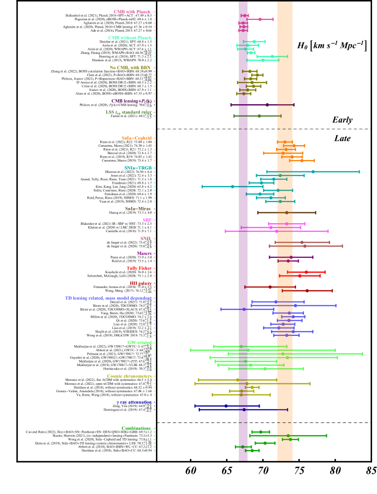
More recently, the joint analysis of lower-redshift, non-CMB, data such as BAO, , SnIa, QSO, HII and GRBs by Cao and Ratra (2022) gives a model-independent determinations of the Hubble constant, (see also Cao et al., 2021b, 2022c, a, 2020, for previous joint analyses).
Many other estimates of have been obtained in the literature within the standard CDM model or in alternative scenarios by using joint analysis (Bonilla et al., 2021a; Renzi and Silvestri, 2020). In addition, many analyses using various combinations of data assuming a CDM model or a extended model beyond CDM cosmology investigate whether the tension persists (or not). For example Okamatsu et al. (2021) use non-CMB data and specifically adopt the data from BAO, BBN, and SnIa to study the tension. They show that this tension exists in a broad framework beyond the standard CDM model.
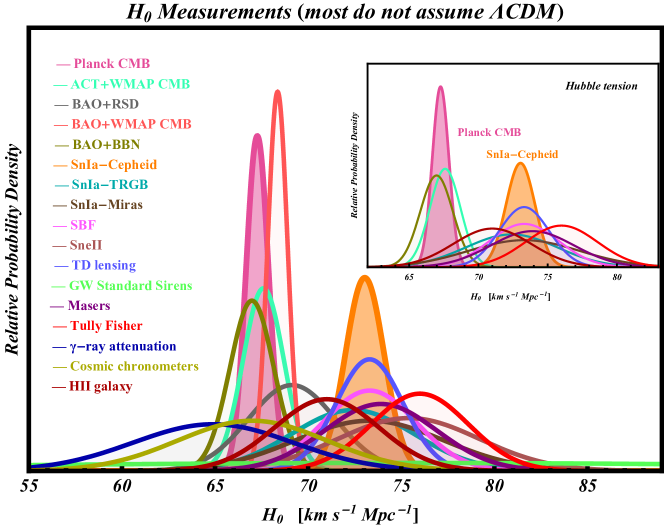
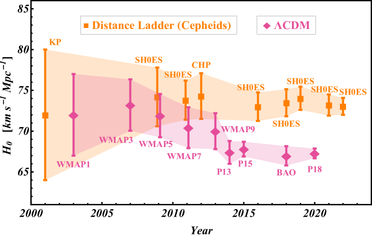
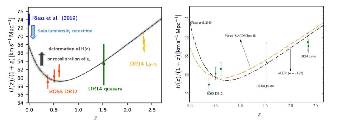
II.1.11 The current status - Historic evolution
Hubble’s initial value in 1929 for the expansion rate, now called the Hubble constant, was approximately . From the 1970s, through the 80s and into the 90s the value of was estimated to be between 50 and 100 (Tully, 1988). Of interest is the historical Hubble constant debate between, for example, long series of papers by Gérard de Vaucouleurs, who claimed that the value of is (e.g. de Vaucouleurs and Peters, 1985; de Vaucouleurs, 1986), and Allan Sandage , who claimed the value is (Sandage and Tammann, 1975, 1984) (see Turner, 2022, for a historical review).
During the last decades there has been remarkable progress in measuring the Hubble constant. The available technology and measurement methods determine the accuracy of this quantity. The Hubble constant as a function of publication date, using a set of different methods is shown in Fig. 12. The values of determined in the late Universe with a calibration based on the Cepheid distance scale and the derived values of from analysis of the CMB anisotropy spectrum data are shown. The uncertainties in these values have been decreasing for both methods and the recent measurements disagree beyond .
Furthermore the comoving Hubble expansion rate as a function of redshift obtained from the Planck CMB is shown in Fig. 13 along with a few relevant data-points demonstrating the Hubble tension.
The basic strategic questions emerge
These important Hubble tension questions will be discussed in the next subsection.
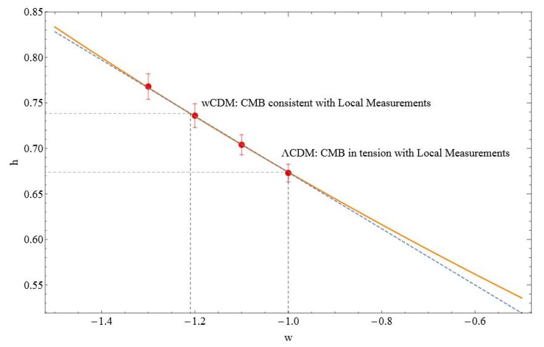
II.2 Theoretical models
A wide range of models have been used to address the tension by introducing additional degrees of freedom to CDM model where additional parameters are allowed to vary such as quintessence (Fujii, 1982; Ford, 1987; Wetterich, 1995, 1988; Ratra and Peebles, 1988; Chiba et al., 1997; Ferreira and Joyce, 1997, 1998; Copeland et al., 1998; Caldwell et al., 1998; Zlatev et al., 1999; Tsujikawa, 2013; Scherrer, 2022; Steinhardt et al., 1999; Liddle and Scherrer, 1999), in which a scalar field plays the role of dark energy or modified gravity (Esposito-Farese and Polarski, 2001; Amendola et al., 2007; Fay et al., 2007; Nojiri and Odintsov, 2007; Perivolaropoulos, 2005; Boisseau et al., 2000), in which General Relativity is modified on cosmological scales (see Copeland et al., 2006; Bamba et al., 2012, for a review).
The extensions of CDM model which can be used to resolve the Hubble constant tension fall into two categories: models with late time and models with early time modification (in the epoch before the recombination) (see Verde et al., 2019; Di Valentino et al., 2021c; Schöneberg et al., 2021, for a review).
The models with late time modification can be divided in four broad classes: deformations of the Hubble expansion rate at late times (e.g. late time phantom dark energy Alestas et al., 2020a; Di Valentino et al., 2016b), deformations of the Hubble expansion rate with additional interactions/degrees of freedom (e.g. interacting dark energy Di Valentino et al. 2017b; Yang et al. 2020f and decaying dark matter Berezhiani et al. 2015), deformations of the Hubble expansion rate due to inhomogeneous/anisotropic modifications (e.g. inhomogeneous causal horizons Fosalba and Gaztañaga, 2020) and transition/recalibration of the SnIa absolute luminosity (Kazantzidis and Perivolaropoulos, 2020) (or combination of the previous classes e.g. late phantom transition Alestas et al., 2021b).
Model selection statistical tools and approaches include the Akaike Information Criterion (AIC) (Akaike, 1974), the Bayesian Information Criterion (BIC) (Schwarz, 1978) and the Deviance Information Criterion (DIC) (Spiegelhalter et al., 2002) and Bayesian model comparison (e.g. Nesseris and Garcia-Bellido, 2013; Saini et al., 2004; Mehrabi and Said, 2022; Keeley and Shafieloo, 2021; Koo et al., 2022). These tools have been developed and used to test, discriminate and compare the proposed models (Liddle, 2004, 2007; Arevalo et al., 2017; Kerscher and Weller, 2019) (see also Abdalla et al., 2022, for a list of statistical tools).
II.2.1 Late time deformations of the Hubble expansion rate
These late time models for the solution of the Hubble tension use a late time smooth deformation of the Hubble expansion rate Planck18/CDM so that it can match the locally measured value of while keeping the radius of the sound horizon at the last scattering surface (see Subsection II.1.2). Many of these models effectively fix the comoving distance to the last scattering surface and the matter energy density to values consistent with Planck/CDM to maintain consistency with the CMB anisotropy spectrum while introducing late time phantom dark energy to deform so that it matches the local measurements of . The required phantom behavior of such deformations can not be provided by minimally coupled quintessence models and therefore such models have been shown to be unable to resolve the Hubble tension (Banerjee et al., 2021a; Lee et al., 2022). These models have three problems
-
•
They tend to worsen the fit to low z distance probes such as BAO and SnIa (e.g. Alestas et al., 2020a)
-
•
They tend to worsen level of the growth tension (Alestas and Perivolaropoulos, 2021).
- •
Thus, these models can not fully resolve the Hubble tension (see also Alestas et al., 2022a, 2021a; Yang et al., 2021d; Benevento et al., 2020; Efstathiou, 2021; Arendse et al., 2020; Theodoropoulos and Perivolaropoulos, 2021; Krishnan et al., 2021b; Bernal et al., 2021; Vagnozzi et al., 2021c; Cai et al., 2022b, a; Escamilla-Rivera et al., 2021; Benisty et al., 2022b).
Physical models where the deformation of may be achieved include the following: phantom dark energy (e.g. Alestas et al., 2020a) (see in Paragraph II.2.1.1), running vacuum model (e.g. Sola and Stefancic, 2006) (see in Paragraph II.2.1.2), phenomenologically emergent dark energy (Li and Shafieloo, 2019) (see in Paragraph II.2.1.3), vacuum phase transition (e.g. Di Valentino et al., 2018b) (see in Paragraph II.2.1.4), phase transition in dark energy (e.g. Khosravi et al., 2019) (see in Paragraph II.2.1.5). Plethora of late dark energy models with an equation of state ( or ) both constant or dynamical with redshift (e.g. Martinelli and Tutusaus, 2019) were proposed to address the Hubble tension. Recently, using a model-independent approach and a fully analytical analysis Heisenberg et al. (2022a, b) derive a set of necessary conditions that any late dark energy model must satisfy in order to potentially address both the Hubble and the growth tensions. In particular, solving the tension requires at some and solving both the and tensions demands time-varying dark energy equation of state which cross the phantom divide. However Alestas and Perivolaropoulos (2021) have shown that deformation approaches to the Hubble tension tend to worsen the growth tension.
The following models may be classified in this class of theories: the holographic dark energy (Guo et al., 2019; Dai et al., 2020; Colgáin and Sheikh-Jabbari, 2021; van Putten, 2017, 2019; da Silva and Silva, 2021a; Hernández-Almada et al., 2021; Adhikary et al., 2021), the considering Chevallier - Polarski - Linder (CPL) (Chevallier and Polarski, 2001; Linder, 2003; Kitazawa, 2020) parameterization (Yang et al., 2019c), the considering dependence on non-vanishing spatial curvature (Miao and Huang, 2018), the phantom brane dark energy (Alam et al., 2017b; Bag et al., 2021), the negative cosmological constant (Visinelli et al., 2019; Calderón et al., 2021; Sen et al., 2021), the negative dark energy (Dutta et al., 2020), the graduated dark energy (Akarsu et al., 2020), the simple-graduated dark energy (Acquaviva et al., 2021), the CDM model (sign-switching) (Akarsu et al., 2021), the transitional dark energy (Keeley et al., 2019), the frame dependent dark energy (Adler, 2019), the running with redshift (Dainotti et al., 2021; Krishnan et al., 2021a), the varying gravitational constant (Sakr and Sapone, 2022), the deviation from the cold dark matter (Elizalde et al., 2021) and the phantom crossing (Di Valentino et al., 2021d). For example in the case of the holographic dark energy model (Dai et al., 2020) and phantom crossing (Di Valentino et al., 2021d) models the tension on appears to be significantly alleviated within even though the three problems mentioned above do remain.
II.2.1.1 Phantom dark energy:
The deformation of through the implementation of late time phantom dark energy (Alestas et al., 2020a; Di Valentino et al., 2016b, 2017a, 2020e; Vagnozzi, 2020; Huang and Wang, 2016) can address the Hubble tension as shown in Fig. 13.
The analysis by Alestas et al. (2020a) indicates that mildly phantom models with mean equation of state parameter have the potential to alleviate this tension. It was shown that the best fit value of in the context of the CMB power spectrum is degenerate with a constant equation of state parameter . The CMB anisotropy spectrum was shown to be unaffected when changing provided that specific parameter combinations remain unchanged. These cosmological parameters fix to high accuracy the form of the CMB anisotropy spectrum. The values of these parameters as determined by the Planck/CDM CMB temperature power spectrum are the following (Aghanim et al., 2020e).
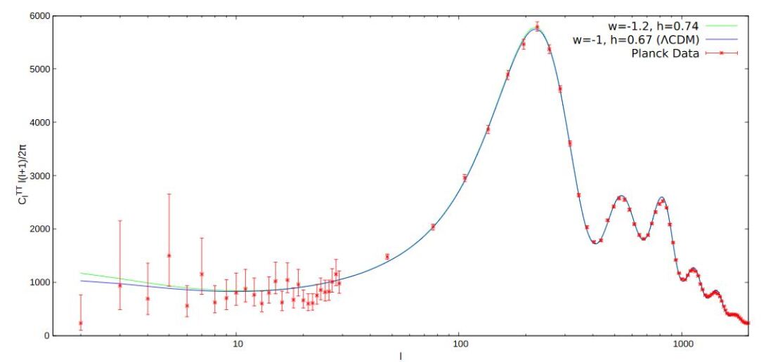
| (56) | |||
| (57) | |||
| (58) | |||
| (59) | |||
| (60) |
where is the energy density of component and is the comoving angular diameter distance.
Using the Eq. (9) the comoving angular diameter distance to the recombination surface is ()
| (61) |
where is the redshift of recombination and is the dimensionless Hubble parameter which in general takes the form
| (62) |
where and determines the evolution of dark energy.
In the context of a simple one parameter parametrization where the equation of state remains constant in time and redshift (wCDM model), takes the simple form
| (63) |
If the four energy densities Eqs. (56), (57), (58) and (59) and the observed value of the comoving angular diameter Eq. (60) are fixed then they provide the analytically predicted best fit value of the Hubble parameter (or ) given the dark energy equation of state parameter where ,… are the parameters entering the parametrization. Thus assuming a flat Universe () and solving the following equation with respect to
| (64) |
it is straightforward to derive the degeneracy function shown in Fig. 14 (continuous orange line). In the range , is approximated as a straight line (dashed blue line in Fig. 14)
| (65) |
For , this linear degeneracy equation leads to the best fit dimensionless Hubble constant as expected while for the corresponding predicted CMB best fit is which is consistent with the value obtained by local distance ladder measurements. The invariance of the CMB power spectrum when the cosmological parameters are varied along the above described degeneracy directions is shown in Fig. 15. This method of Alestas et al. (2020a) can be used to find general degeneracy relations between and and fixing gives infinite , forms that can potentially resolve the problem if they can also properly fit the low date (e.g. BAO, SnIa, Cepheid value of absolute luminosity ). Low distance data (BAO and SnIa) will determine which one of these forms is observationally favored. However, none of these forms can provide a quality of fit to low z data equally good or better than CDM despite the introduced additional parameters. In addition, these models suffer from the other two problems mentioned above (worse growth tension and lower value of SnIa absolute magnitude).
II.2.1.2 Running vacuum model:
The running vacuum models (RVM) (Sola and Stefancic, 2006, 2005; Shapiro et al., 2005; Shapiro and Sola, 2008, 2009; Basilakos et al., 2012; Perico et al., 2013; Basilakos et al., 2016; Perico et al., 2013; Tsiapi and Basilakos, 2019; Banerjee et al., 2021c; Farrugia et al., 2020; Basilakos et al., 2020a; Lima et al., 2013; Moreno-Pulido and Solà, 2020; Basilakos et al., 2019; Mavromatos, 2021a; Rezaei et al., 2021; Mavromatos and Solà Peracaula, 2021a, b; Shapiro and Sola, 2004; Basilakos et al., 2020b) (see Peracaula, 2022; Sola, 2011, 2013; Solà and Gómez-Valent, 2015; Sola, 2015; Solà, 2016; Mavromatos, 2022, 2021b, for a review) attempts to address both the Hubble constant tension (Solà et al., 2017b) and the growth tension using a mechanism that has common features with the IDE models (e.g. Solà et al., 2015, 2017a; Gómez-Valent and Solà, 2017; Gómez-Valent and Solà Peracaula, 2018; Solà Peracaula, 2021; Solà Peracaula et al., 2021) (for relaxing the growth tension, see Subsection III.1.2).
The RVM of the cosmic evolution is well motivated by the generic idea of renormalization group formalism which is used in Quantum Field Theory (QFT) (Sola, 2008; Shapiro and Sola, 2000, 2002) (see also Moreno-Pulido and Solà, 2020; Moreno-Pulido and Peracaula, 2022, for a approach using adiabatic regularization and renormalization techniques). In the RVM the cosmological constant, the corresponding vacuum energy density and pressure are assumed to be functions of the Hubble rate e.g. a power series of the Hubble rate and its cosmic time derivative with even time derivatives of the scale factor (Gómez-Valent et al., 2015)
| (66) |
and respectively.
For the current Universe the vacuum energy density can be written in the relatively simple form (e.g. Solà and Gómez-Valent, 2015; Gómez-Valent et al., 2015; Solà Peracaula et al., 2018; Solà et al., 2017b)
| (67) |
where (with the current value) is an integration constant which is fixed by the boundary condition (with the current value) and is a dimensionless running parameter which characterizes the dynamics of the vacuum at low energy. For the vacuum energy remains constant at all times and for the vacuum energy density decreases with the time. In QFT the running parameter is (Sola, 2008) but in RVM it has been treated as a free parameter by fitting to the observational data (e.g. Gómez-Valent et al., 2015; Solà Peracaula et al., 2018).
II.2.1.3 Phenomenologically emergent dark energy:
Phenomenologically emergent dark energy (PEDE) is a zero freedom dark energy scenario proposed by Li and Shafieloo (2019). In this model the dark energy density has the following form
| (68) |
where .
The dark energy in this model has no effective presence in the past and emerges at the later times and with the same number (six) of parameters compared to the spatially flat CDM scenario. It has the potential for alleviating the tension (Li and Shafieloo, 2019; Pan et al., 2020b; Yang et al., 2021a; Liu and Miao, 2020; Rezaei et al., 2020; Yang et al., 2021b; Di Valentino et al., 2021a). The generalised emergent dark energy (GEDE) model has one extra dimensionless free parameter including both CDM model as well as the PEDE model as two of its special limits introduced by Li and Shafieloo (2020). In the GEDE model the dark energy density has the following form (Yang et al., 2021c)
| (69) |
where is the transition redshift where dark energy density equals to matter density. For and this model recovers CDM and PEDE model respectively. Using the latest observational Hubble dataset Hernández-Almada et al. (2020) revisited and constrained the free parameters of the PEDE and GEDE models.
Other versions of the PEDE model are the Modified Emergent Dark Energy (MEDE) (Benaoum et al., 2022) and the Transitional Dark Energy (TDE) (Zhou et al., 2022) models. The MEDE model with one extra degree of freedom reduces the Hubble tension to (Benaoum et al., 2022) even though it also suffers from the three problems of the late time deformation models.
II.2.1.4 Vacuum phase transition:
Vacuum phase transition (Di Valentino et al., 2018b, 2020b, 2021e, 2021a) based on vacuum metamorphosis (VM) or vacuum cold dark matter model (VCDM) (Parker and Raval, 2000; Parker and Vanzella, 2004; Caldwell et al., 2006) has the potential to address the tension. This mechanism with six free parameters as the spatially flat CDM. It also assumes a phase transition in the nature of the vacuum similar to Sakharov’s induced gravity (Sakharov, 1991). The phase transition occurs when the evolving Ricci scalar curvature becomes equal to the value of scalar field mass squared (Di Valentino et al., 2018b)
| (70) |
where the dot corresponds to the derivative with respect to cosmic time . After the transition the Ricci scalar curvature remains constant with and this changes the expansion rate below () due to the phase transition
| (71) |
| (72) |
where and is the transition redshift.
II.2.1.5 Phase transition in dark energy:
-
•
Phase transition in dark energy explored by Khosravi et al. (2019); Banihashemi et al. (2019, 2020); Moshafi et al. (2021) can address the Hubble tension. Generalizing this model by assigning a more realistic time evolution of dark energy Banihashemi et al. (2021) propose the critically emergent dark energy (CEDE) model.
In Farhang and Khosravi (2021) the form of phase transition parametrized phenomenologically by a hyperbolic tangent function. This scenario for dark energy is similar used independently as PEDE and GEDE.
-
•
Late dark energy (LDE) transition (Benevento et al., 2020) at redshifts can reduce the Hubble tension. This class of deformation models has a more intense form of the third problem of the deformation class as they predict a significantly lower value of the SnIa absolute magnitude than the other deformation models (Alestas et al., 2021b; Camarena and Marra, 2021).
In this scenario the true Hubble constant is given by (Mortonson et al., 2009; Benevento et al., 2020)
(73) where is the prediction for a flat CDM model in the context of a CMB sound horizon calibration.
In Benevento et al. (2020); Dhawan et al. (2020) it was shown that this model can not fully resolve the Hubble problem as it would imply a transition in the SnIa apparent magnitude which is not observed. These models however become viable in the context of a SnIa absolute magnitude transition (Alestas et al., 2021b; Marra and Perivolaropoulos, 2021).
II.2.2 Deformations of the Hubble expansion rate with additional interactions/degrees of freedom
There exist several varieties of the models for the solution of the Hubble tension which use deformations of the Hubble expansion rate with additional interactions/degrees of freedom. For example the interacting dark energy models (e.g. Di Valentino et al., 2017b; Yang et al., 2020f) (see in Paragraph II.2.2.1) with an extra non-gravitational interaction between the components of the Universe and the decaying dark matter models (e.g. Berezhiani et al., 2015) (see in Paragraph II.2.2.2) with additional degrees of freedom are able to alleviate the Hubble constant tension.
The following models may be classified in this class of theories: multi-interacting dark energy (Lucca, 2021), new interacting dark energy (Gao et al., 2021), interacting vacuum energy (Kumar, 2021), metastable dark energy (Li et al., 2019c; Yang et al., 2020e), Quintom dark energy (Panpanich et al., 2021), cannibal dark matter (Buen-Abad et al., 2018a), baryons-dark energy interacting (Jiménez et al., 2020) (see also Vagnozzi et al., 2020; Ferlito et al., 2022), swampland conjectures (Ó Colgáin et al., 2019; Colgáin and Yavartanoo, 2019; Agrawal et al., 2021), nonlocal gravity (Belgacem et al., 2018, 2020a), late time transitions in the quintessence field (Di Valentino et al., 2019a), Galileon gravity (Renk et al., 2017; Zumalacarregui, 2020; Peirone et al., 2019; Frusciante et al., 2020; Heisenberg and Villarrubia-Rojo, 2021), gravity (Odintsov et al., 2021; D’Agostino and Nunes, 2020; Wang, 2021; Jiménez Cruz and Escamilla-Rivera, 2021), gravity (Nunes, 2018; Wang and Mota, 2020; Ren et al., 2021; Cai et al., 2020; Hashim et al., 2021; Briffa et al., 2020; Benisty et al., 2022a; Bahamonde et al., 2022; Ren et al., 2022), gravity (Escamilla-Rivera and Levi Said, 2020), gravity (Mandal et al., 2020), Brans-Dicke gravity (Solà Peracaula et al., 2019, 2020), minimal theory of massive gravity (de Araujo et al., 2021), scale–dependent gravity (Alvarez et al., 2021), unimodular gravity (Perez et al., 2021; Linares Cedeño and Nucamendi, 2021), the screened fifth forces (Desmond et al., 2019; Desmond and Sakstein, 2020), the minimally modified gravity (De Felice et al., 2021), the Lifshitz cosmology (Berechya and Leonhardt, 2021), the Milne cosmology (Vishwakarma, 2020), 4D Gauss-Bonnet gravity (Wang and Mota, 2021), the generalized Chaplygin gas (Yang et al., 2019f), the unified cosmologies (Yang et al., 2019e), the -gravity (Gurzadyan and Stepanian, 2019, 2021), the -model (Benetti et al., 2019, 2021), the bulk viscous cosmology (Elizalde et al., 2020; da Silva and Silva, 2021b; Yang et al., 2019b; Normann and Brevik, 2021) and the surface tension hypothesis (Ortiz, 2020). For instance in the case of the metastable dark energy (Yang et al., 2020e), generalized Chaplygin gas (Yang et al., 2019f) and Galileon gravity (Renk et al., 2017) models the tension on appears to be significantly alleviated to within about even though the there problems of the deformation models remain to be addressed.
II.2.2.1 Interacting dark energy:
In the cosmological interacting dark energy (IDE) models (Nunes et al., 2022; Linton et al., 2021; Hogg and Bruni, 2021; Mancini and Pourtsidou, 2021; Sharma and Sur, 2022; Carrilho et al., 2021b, a; Amendola, 2000; Wang and Meng, 2005; Salvatelli et al., 2013; Costa et al., 2014; Pourtsidou et al., 2013; Pettorino, 2013; Salvatelli et al., 2014; Kumar and Nunes, 2016; Xia and Wang, 2016; Kumar and Nunes, 2017; Van De Bruck and Mifsud, 2018; Di Valentino et al., 2017b; Yang et al., 2017c, 2019g, 2018c, 2018a, 2018b; Li et al., 2019b; An et al., 2019; Gonzalez et al., 2018; Kumar et al., 2019; Pan et al., 2019b; Yang et al., 2019a, 2020f; Gómez-Valent et al., 2020; Aljaf et al., 2021; Di Valentino et al., 2020c; Martinelli et al., 2019; Di Valentino et al., 2021b; Yao and Meng, 2020, 2021; Lucca and Hooper, 2020; Yang et al., 2020d, c; Amirhashchi and Yadav, 2020; Johnson et al., 2022; Pan et al., 2019a) (see Wang et al., 2016a; Bolotin et al., 2014, for a review) the dark components of the Universe i.e dark matter (DM) and dark energy (DE) have an extra non-gravitational interaction. The IDE model was proposed to address the coincidence problem (e.g. Comelli et al., 2003; Huey and Wandelt, 2006; Cai and Wang, 2005; Pavon and Zimdahl, 2005; Zhang, 2005; del Campo et al., 2006; Berger and Shojaei, 2006; del Campo et al., 2009; He and Wang, 2008). In addition the interaction between the dark fluids has been shown to be effective in substantially alleviating the Hubble constant tension (Yang et al., 2018a, b; Di Valentino et al., 2017b, 2020d; Pan et al., 2019a; Kumar and Nunes, 2016; Yang et al., 2020f; Lucca and Hooper, 2020; Wang et al., 2021; Gariazzo et al., 2021; Nunes and Di Valentino, 2021; Guo et al., 2021; Pan et al., 2020c) or in addressing the structure growth tension between the values inferred from the CMB and the WL measurements (Pourtsidou and Tram, 2016; An et al., 2018; Barros et al., 2019; Camera et al., 2019) (see Subsection III.1.2) or in solving the two tensions simultaneously (Kumar and Nunes, 2017; Kumar et al., 2019; Di Valentino et al., 2020c).
In IDE cosmology assuming spatially flat Friedmann-Lematre-Roberson-Walker background and pressureless dark matter () the equations of evolution of the dark matter and dark energy densities and respectively are given by (Gavela et al., 2009)
| (74) |
| (75) |
where the dot corresponds to the derivative with respect to cosmic time , is the equation of state of dark energy and represents the interaction rate between the dark sectors (i.e. the rate of energy transfer between the dark fluids). For energy flows from dark matter to dark energy, whereas for the energy flow is opposite.
These models combine the deformation of with an extra modification of the growth rate of perturbations due to the tuned evolution of induced by the interaction term . This additional tuning allows for a simultaneous improvement of the growth tension in contrast to models that involve a simple deformation.
Various phenomenological IDE models were proposed in the literature where the rate of the interaction has a variety of possible functional forms (Pan et al., 2020a). For example in some classes of IDE models the rate of the interaction is proportional to the energy density of dark energy (Kumar and Nunes, 2017; Kumar et al., 2019; Yang et al., 2020f; Di Valentino et al., 2020c) or cold dark matter (Kumar and Nunes, 2016) (where is a constant and in the CDM cosmology), or some combination of the two. Note that in the case of functional form instabilities develop in the dark sector perturbations at early times (He et al., 2009).
II.2.2.2 Decaying dark matter:
Decaying dark matter into dark radiation (i.e. an unknown relativistic species that is not directly detectable), which has been first analysed by Ichiki et al. (2004) and studied by Chen:2020iwm; Chudaykin et al. (2018); Bjaelde et al. (2012); Wang et al. (2014); Anchordoqui et al. (2015); Xiao et al. (2020); Choi et al. (2020b, a); Nygaard et al. (2021), provides a promising scenario to relieve the Hubble constant tension (e.g. Berezhiani et al., 2015). Also, it has been shown that this scenario can resolve the growth tension (Enqvist et al., 2015; Abellán et al., 2022) or the two tensions simultaneously (Pandey et al., 2020) by a similar mechanism as in the IDE models. However, using the Planck data the analysis of the model by Poulin et al. (2016); Chudaykin et al. (2016) has shown that the cosmological tensions are only slightly alleviated (see Bringmann et al., 2018, for a different result).
In these models assuming spatially flat Friedmann-Lematre-Roberson-Walker Universe, pressureless dark matter, and equation of state of dark radiation , the equations of evolution of the dark matter and dark radiation densities and respectively are given by (Gavela et al., 2009)
| (76) |
| (77) |
where is the decay rate of dark matter particles (with the particle’s lifetime). In the literature a variety of possible functional forms of the decay rate has been explored (Enqvist et al., 2015; Lesgourgues et al., 2016; Poulin et al., 2016; Bringmann et al., 2018). For example in some cases the decay rate is proportional to the Hubble rate, (Pandey et al., 2020). Constraints on the decay rate of dark matter have been obtained by the analysis of Ando and Ishiwata (2015); Enqvist et al. (2015).
A model with decaying dark matter into dark radiation in early/late Universe ( / , where is the time of last scattering) increases/decreases the expansion rate at high/low redshifts as it predicts a smaller matter content and a larger radiation content as time evolves (the early/late Universe is dominated by the radiation/matter and the dark radiation density decreases more rapidly than the matter density, and ). In the case of , the faster cosmological expansion decreases the scale of the sound horizon in Eq. (26) because the baryon-to-photon ratio, and thus in Eq. (27), is tightly constrained by CMB fluctuations and BBN (Ade et al., 2016e). In the context of the degeneracy shown in Eq. (28) the lower scale of the sound horizon yields a larger value of . In the case of , the lower dimensionless normalized Hubble rate in the late-time leads to a larger value of since and must be kept fixed in Eq. (28). Accordingly, both early and late decaying dark matter model are able to alleviate the Hubble constant tension (see Anchordoqui, 2021; Anchordoqui et al., 2022, for a detailed discussion).
There are alternative decaying dark matter models such as the light dark matter (Alcaniz et al., 2021), the dynamical dark matter (Desai et al., 2020), the many-body or -body decaying cold dark matter scenarios (Blackadder and Koushiappas, 2014) and the decaying warm dark matter scenario (Blinov et al., 2020). In the -body decaying cold dark matter scenario the decaying dark matter produces two particles, one massive warm dark matter particle and one massless relativistic particle (dark radiation). This scenario can address the Hubble constant tension (Vattis et al., 2019; Clark et al., 2021b; Haridasu and Viel, 2020) and the growth tension (Abellán et al., 2021).
A self-interacting dark matter model with a light force mediator coupled to dark radiation studied by Binder et al. (2018); Hryczuk and Jodłowski (2020). This model can simultaneously reduce the tension between CMB and low-redshift astronomical observations of and .
Jaeckel and Yin (2021a) pointed out that a dark particle from reheating (Jaeckel and Yin, 2021b) can alleviate the tension through its decay to relativistic component which contributes to the dark radiation.
Recently, Ly- constraints on possible models of dark-matter physics have been evaluated by Dienes et al. (2021). In particular the Ly- bounds on different classes of dark-matter velocity distributions have been obtained.
II.2.3 Deformations of the Hubble expansion rate with inhomogeneous/anisotropic modifications
Models where the cosmological principle and the FLRW metric are relaxed by considering inhomogeneous/anisotropic modifications have the potential to resolve the Hubble problem (Kasai and Futamase, 2019). Physical models where the deformation of may be achieved with inhomogeneous/anisotropic modifications, include the following: Chameleon dark energy (e.g. Cai et al., 2021) (see in Paragraph II.2.3.1), cosmic voids (Wu and Huterer, 2017) (see also Paragraph II.2.3.2) and inhomogeneous causal horizons (Fosalba and Gaztañaga, 2020) (see also Paragraph II.2.3.3), charged dark matter (Jiménez et al., 2021; Beltran Jimenez et al., 2020, 2021), Bianchi type I spacetime (Akarsu et al., 2019) and emerging spatial curvature (Heinesen and Buchert, 2020; Bolejko, 2018).
II.2.3.1 Chameleon dark energy:
Chameleon dark energy (Khoury and Weltman, 2004b, a) (see also Brax et al., 2007; Banerjee et al., 2010; Das and Banerjee, 2008; Brax et al., 2010; Wang et al., 2012; Upadhye et al., 2012; Khoury, 2013; Vagnozzi et al., 2021d; Benisty and Davis, 2022) attempts to address the Hubble constant tension by introducing a cosmic inhomogeneity in the Hubble expansion rate at late-time from the chameleon field coupled to the local matter overdensities (Cai et al., 2021). This field trapped at a higher potential energy density acts as an effective cosmological constant and results in a faster local expansion rate than that of the background with lower matter density.
II.2.3.2 Cosmic voids:
In cosmic void models the local departs significantly from the cosmic mean because of the presence of an under-dense region (local void) (Lombriser, 2020). However in Wu and Huterer (2017); Kenworthy et al. (2019) it was shown that this alternative theory is inconsistent with current observations. The analysis was based on the assumption of the validity of standard CDM and a study of the sample variance in the local measurements of the Hubble constant this alternative theory has been shown inconsistent with current observations. Wu and Huterer (2017) estimated that the required radius of void to resolve the tension in is about and density contrast of which is inconsistent at with the CDM cosmology (Kenworthy et al., 2019; Haslbauer et al., 2020).
In the context of this inconsistency, Haslbauer et al. (2020) considered a cosmological Milgromian dynamics or modified Newtonian dynamics (MOND) model (Milgrom, 1983) with the presence of sterile neutrinos252525Sterile neutrinos are a special kind of neutrino with right handed chirality that might interact only through gravity (Dodelson and Widrow, 1994; Boyarsky et al., 2009) (see Kusenko, 2009; Abazajian et al., 2012; Drewes, 2013, for a review). They have been proposed to resolve some anomalies in neutrino data. to show that the Keenan-Barger-Cowie (KBC) void262626The KBC void (Keenan et al., 2013) is a large local underdensity between and (i.e. ) around the Local Group. has the potential to resolve the Hubble tension.
II.2.3.3 Inhomogeneous Causal Horizons:
Fosalba and Gaztañaga (2020) proposed a simple solution to the tension based on causally disconnected regions of the CMB temperature anisotropy maps from Planck (Aghanim et al., 2020b). It was pointed out that CMB maps show ’causal horizons’ where cosmological parameters have distinct values. This could be justified by the fact that these regions of the Universe have never been in causal contact. Thus it was shown that the Hubble constant takes values which differ up to among different causally disconnected regions. These cosmological parameter inhomogeneities are in agreement with the model of the Universe proposed in Gaztanaga (2020) (see also Gaztanaga 2021a, b, 2022 for details) where the cosmological constant is simply formulated as a boundary term in the Einstein equations and where ’Causal Horizons’ naturally arise. Thus if there are similar ’causal horizons’ in the local universe (i.e, ), then variations between the local and high-z measures of are indeed to be expected (Fosalba and Gaztañaga, 2020).
II.2.4 Late time modifications - Transition/Recalibration of the SnIa absolute luminosity
This class of models can address the problems of the deformation models (especially the low problem) by assuming a rapid variation (transition) of the SnIa intrinsic luminosity and absolute magnitude due e.g. to a gravitational physics transition at a redshift (Marra and Perivolaropoulos, 2021; Alestas et al., 2021b, a).
II.2.4.1 Gravity and evolution of the SnIa intrinsic luminosity:
As shown in the recent analysis by Kazantzidis and Perivolaropoulos (2020) there are abnormal features which may be interpreted as evolution of the measured parameter combination (see Section II.1.1). This measured parameter combination in Eq. (19) depends on the absolute magnitude and on the Hubble constant ( and are degenerate parameters). Any variation of the parameter is due to a variation of which could be induced by a varying (where is the local value of the Newton’s constant ). If the calibrated SnIa absolute magnitude were truly constant then the parameter should also be constant (independent of redshift).
A possible variation of the absolute magnitude and equivalently of the absolute luminosity
| (78) |
could be due to a variation of the fine structure constant or the Newton’s constant .
If the absolute luminosity is proportional to the Chandrasekhar mass we have (Garcia-Berro et al., 1999; Gaztanaga et al., 2002)
| (79) |
Thus will increase as decreases272727 Adopting a semi-analytical model which takes into account the stretch of SnIa light curves but assumes fixed mass of Ni, obtains SnIa light curves in the context of modified gravity Wright and Li (2018) have claimed that will increase as increases..
Under these assumptions, we obtain
| (80) |
where corresponds to a reference local value of the absolute magnitude and is the relative effective gravitational constant (with the strength of the gravitational interaction and the locally measured Newton’s constant).
Then, the Eq. (19) takes the following form
| (81) |
and the apparent magnitude Eq. (20) can be written as
| (82) |
A mild tension at level in the best fit value of was found in between the low-redshfit () data and the full Pantheon dataset in the context of a CDM model. This tension can be interpreted as (Kazantzidis and Perivolaropoulos, 2020)
-
•
a locally higher value of by about , corresponding to a local matter underdensity.
-
•
a time variation of Newton’s constant which implies an evolving Chandrasekhar mass and thus an evolving absolute luminosity L and absolute magnitude M of low z SnIa.
In addition, the oscillating features shown in Fig. 4 hint also to the possibility of evolutionary effects of . As discussed below such evolutionary effects if they exist in the form of a transition may provide a solution to the Hubble and growth tensions.
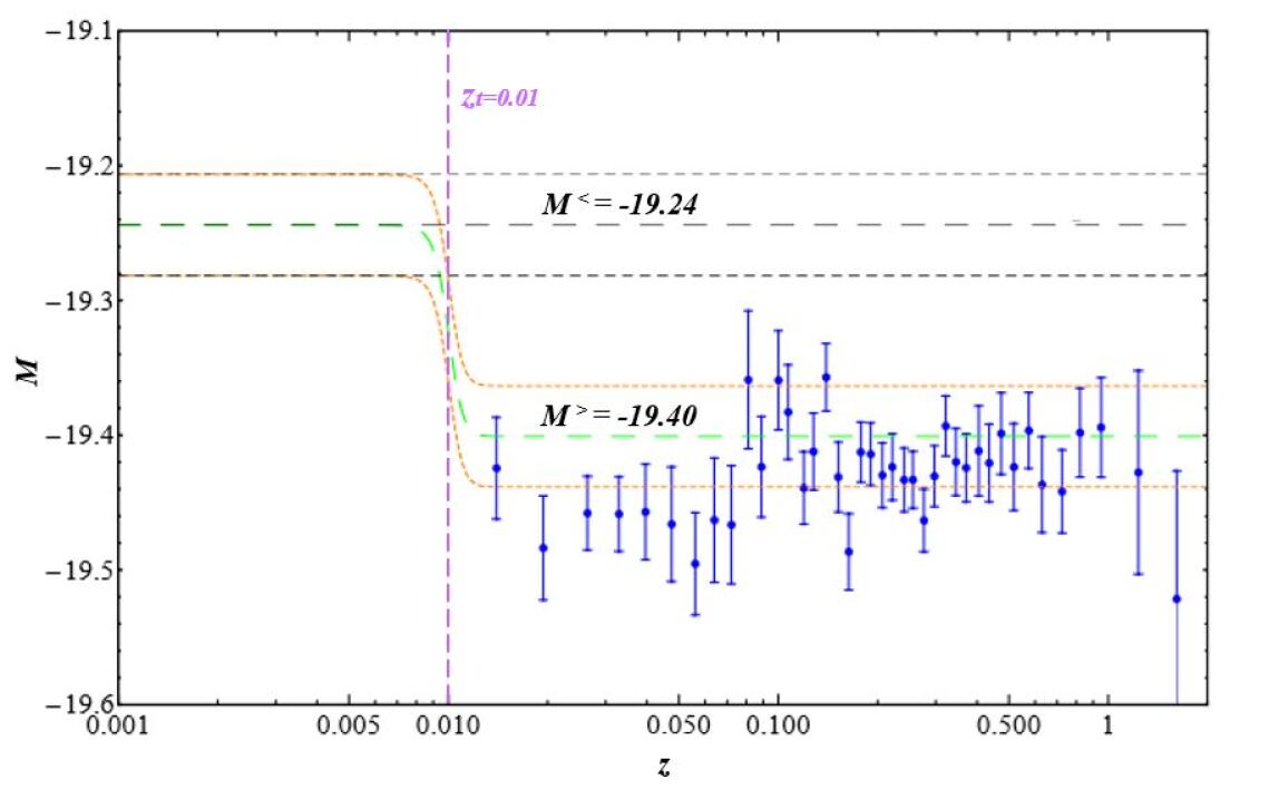
II.2.4.2 Transition of the SnIa absolute magnitude at a redshift :
Recently, Marra and Perivolaropoulos (2021) have proposed that a rapid transition (abrupt deformation) at a transition redshift in the value of the SnIa absolute magnitude of the form
| (83) |
(where is the Heaviside step function) due to a rapid transition of the gravitational constant can address the Hubble tension.
In particular the analysis by Marra and Perivolaropoulos (2021) has shown that a rapid transition in the value of the relative effective gravitational constant at is sufficient to induce the required reduction of
| (84) |
where is the SnIa absolute magnitude of Eq. (22) calibrated by Cepheids at (Camarena and Marra, 2020b, 2021) and is the SnIa absolute magnitude of Eq. (23) using the parametric-free inverse distance ladder of Camarena and Marra (2020a). Fig. 16 shows the Pantheon SnIa absolute magnitudes for a Planck/CDM luminosity distance (Scolnic et al., 2018) obtained from
| (85) |
where are the apparent magnitude datapoints.
The data are in disagreement with the SnIa absolute magnitude calibrated by Cepheids but they become consistent if there is a transition in the absolute magnitude with amplitude (Marra and Perivolaropoulos, 2021). Thus, this class of -transition models avoids the -problem of late time deformation models.
Assuming the power law dependence Eq. (79) and using RSD and WL data (Abbott et al., 2019b; Skara and Perivolaropoulos, 2020; Alestas et al., 2020a) reported a best fit value ( corresponds to and corresponds to ) in the context of a CDM background . The analysis by Marra and Perivolaropoulos (2021) showed that a rapid increase of the effective gravitational constant roughly 150 million years ago can also solve - growth tension.
Recently, Alestas and Perivolaropoulos (2021) have demonstrated that this model has an advantage over both early time and late time deformations of to fully resolve the Hubble tension while at the same time improving the level of the - growth tension. In addition it has the potential to provide equally good fit to low distance probes such as BAO and SnIa as the Planck18/CDM model.
More recently, Perivolaropoulos and Skara (2022) generalized the symmetron screening mechanism282828For reviews of modified gravity theories with screening mechanisms, such as the Vainshtein (Vainshtein, 1972; Arkani-Hamed et al., 2003; Deffayet et al., 2002) and the chameleon (Khoury and Weltman, 2004b, a; Gubser and Khoury, 2004; Brax et al., 2004b, a; Upadhye et al., 2006; Mota and Shaw, 2006, 2007; Brax et al., 2008, 2010) models see (Khoury, 2010; Burrage and Sakstein, 2018; Sakstein, 2013; Brax et al., 2012; Jain and Khoury, 2010; Davis et al., 2012; Hui et al., 2009; Burrage and Sakstein, 2016; Joyce et al., 2015; Brax et al., 2021; Baker et al., 2021; Sakstein, 2018) and for screening effects see (Renevey et al., 2021). (Hinterbichler and Khoury, 2010; Hinterbichler et al., 2011) by allowing for an explicit symmetry breaking of the symmetron potential. The explicit symmetry breaking can create an asymmeron wall network pinned on matter overdensities separating regions with distinct gravitational properties which could constitute a physical mechanism for the realization of gravitational transitions in redshift space that could help in the resolution of the Hubble and growth tensions. Another theoretical model leading to a gravitational transition could include a pressure non-crushing cosmological singularity in the recent past Odintsov and Oikonomou (2022).
II.2.4.3 Late (low-redshift) phantom transition:
The late (low-redshift) phantom transition (Alestas et al., 2021b) is a late time approach involving a combination of the previous two classes: the transition of the SnIa absolute luminosity and the deformation of the Hubble expansion rate . A rapid phantom transition of the dark energy equation of state parameter at a transition redshift of the form
| (86) |
with and a similar transition in the value of the SnIa absolute magnitude of the form
| (87) |
with due to evolving fundamental constants can address the Hubble tension (Alestas et al., 2021b). Where is the Heaviside step function, is the SnIa absolute magnitude Eq. (22) calibrated by Cepheids (Camarena and Marra, 2021, 2020b) at and , are parameters to be fit by the data. Alestas et al. (2021b) find , for which imply a lower value of at (about ) compared to the pure -transition model.
The late (low-redshift) phantom transition (LwMPT) can lead to a resolution of the Hubble tension in a more consistent manner than smooth deformations of the Hubble tension and other types of late time transitions such as the Hubble expansion rate transition (Benevento et al., 2020; Dhawan et al., 2020). Its main advantages include the consistency in the predicted value of the SnIa absolute magnitude M and the potential for simultaneous resolution of the growth tension.
Mortsell et al. (2021a, b); Perivolaropoulos and Skara (2021) have analyzed the color-luminosity relation of Cepheids in anchor galaxies and SnIa host galaxies by identifying the color-luminosity relation for each individual galaxy instead of enforcing a universal color-luminosity relation to correct the NIR Cepheid magnitudes. A systematic brightening of Cepheids at distances larger than about which could be enough to resolve the Hubble tension was found. In addition, Perivolaropoulos and Skara (2021) investigating the effects of variation of the Cepheid calibration empirical parameters (the color-luminosity parameter or the Cepheid absolute magnitude) find hints for the presence of a fundamental physics transition taking place at a time more recent than 100 Myrs ago. The magnitude of the transition lead to value of that is consistent with the CMB inferred value thus eliminating the Hubble tension. The distance range/timescale corresponding to this transition is consistent with solar system history data (Perivolaropoulos, 2022) indicating an increase of the rate of impactors on the Moon and Earth surfaces by about a factor of 2-3 during the past 100Myrs which correspond to (Shoemaker, 1998; Gehrels, 1995; McEwen et al., 1997; Grier et al., 2001; Ward and Day, 2007; Mazrouei et al., 2019; Bottke et al., 2007) and low redshift galaxy surveys data (Alestas et al., 2022b). Such a transition is also consistent with a recent analysis by Alestas et al. (2021a) indicating a transition in the context of the Tully-Fisher data.
In particular, using a robust dataset of 118 Tully-Fisher datapoints Alestas et al. (2021a) have demonstrated that evidence for a transition in the evolution of BTFR appears at a level of more than . Such effect could be interpreted as a transition of the effective Newton’s constant. The amplitude and sign of the gravitational transition are consistent with the mechanisms for the resolution of the Hubble and growth tension discussed above (Marra and Perivolaropoulos, 2021; Alestas et al., 2021b) (see in Perivolaropoulos, 2021b, for a talk of the tensions of the CDM and a gravitational transition ).
II.2.5 Early time modifications of sound horizon
Modifying the scale of sound horizon (i.e. the scale of the standard ruler) by introducing new physics before recombination that deform at prerecombination redshifts can increase the CMB inferred value of (Bernal et al., 2016; Poulin et al., 2018a; Aylor et al., 2019; Knox and Millea, 2020) and thus resolve the Hubble tension. Such deformation may be achieved by introducing various types of additional to the standard model components (see Asadi et al., 2022, for a review). These models have the problem of predicting stronger growth of perturbations than implied by dynamical probes like redshift space distortion (RSD) and weak lensing (WL) data and thus may worsen the - growth tension (Jedamzik et al., 2021; Alestas and Perivolaropoulos, 2021).
A wide range of mechanisms has been proposed for the decrease of the the sound horizon scale at recombination. These mechanisms include the introduction of early dark energy, extra neutrinos or some other dark sector at recombination, features in the primordial power spectrum, modified scenarios of recombination etc. The following models and theories may be classified in this class of mechanisms: early dark energy (e.g. Poulin et al., 2019) (see Paragraph II.2.5.1), dark radiation (e.g. Green et al., 2019) (see Paragraph II.2.5.2), neutrino self-interactions (e.g Kreisch et al., 2020) (see Paragraph II.2.5.3), large primordial non-Gaussianities (Adhikari and Huterer, 2020) (see Paragraph II.2.5.4), Heisenberg’s uncertainty principle (Capozziello et al., 2020) (see Paragraph II.2.5.5), early modified gravity (Braglia et al., 2021) (see Paragraph II.2.5.6), cosmological inflation physics (Tanin and Tenkanen, 2021; Aresté Saló et al., 2021; Hazra et al., 2019; Tram et al., 2017; Di Valentino and Bouchet, 2016; Di Valentino and Mersini-Houghton, 2017; Guo and Zhang, 2017; Chiang and Slosar, 2018; Di Valentino et al., 2018c; Liu and Huang, 2020; Keeley et al., 2020a; Ye et al., 2021a; Takahashi and Yin, 2021a), dark matter - photon coupling (Kumar et al., 2018; Yadav, 2019), dark matter-neutrino interactions (Paul et al., 2021), interacting dark radiation (Blinov and Marques-Tavares, 2020), ultralight dark photon (Flambaum and Samsonov, 2019), primordial black holes (Nesseris et al., 2020; Flores and Kusenko, 2021), primordial magnetic fields (Jedamzik and Saveliev, 2019; Jedamzik and Pogosian, 2020; Thiele et al., 2021), non-standard recombination (Liu et al., 2020a), unparticles dark energy (Artymowski et al., 2021), varying fundamental constants (Franchino-Viñas and Mosquera, 2021; Hart and Chluba, 2018; Sekiguchi and Takahashi, 2021; Hart and Chluba, 2020, 2022), early-time thermalization of cosmic components (Velten et al., 2021), CMB monopole temperature shift (Ivanov et al., 2020a), open and hotter universe (Bose and Lombriser, 2021; Bengaly et al., 2020b), Axi-Higgs cosmology (Fung et al., 2021b, a), string Cosmology (Anchordoqui, 2020; Anchordoqui et al., 2020) and dark massive vector fields (Anchordoqui and Perez Bergliaffa, 2019). In this list of proposed cosmological models the tension on is alleviated with a significance ranging from the to the level.
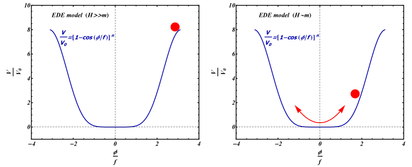
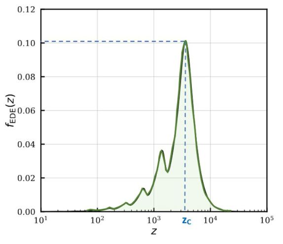
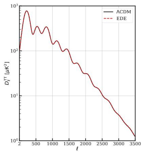
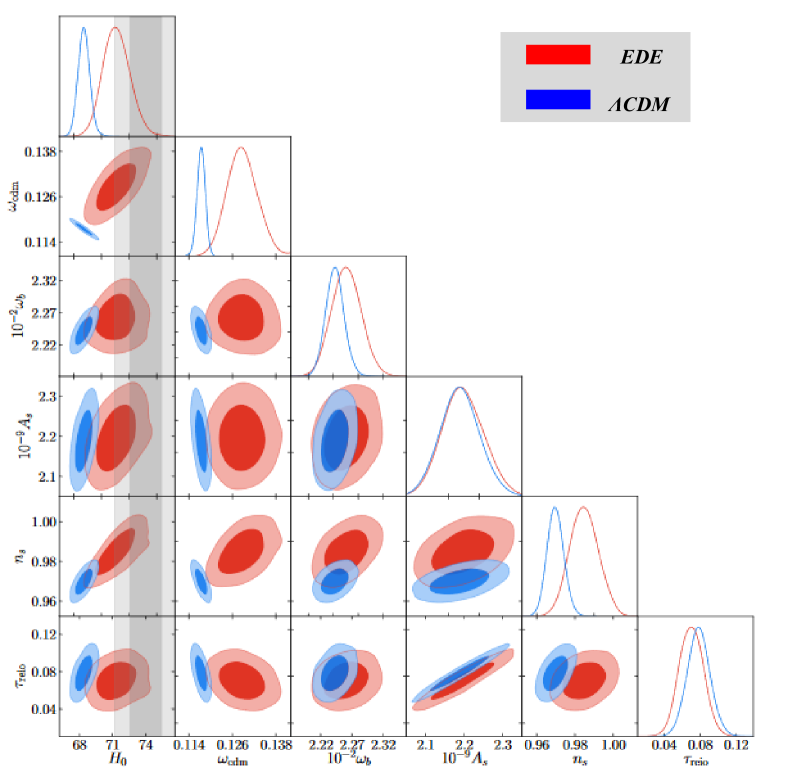
II.2.5.1 Early dark energy:
In the early dark energy (EDE) model (Klypin et al., 2021; Herold et al., 2021; La Posta et al., 2021; Gómez-Valent et al., 2021; Fondi et al., 2022; Hill et al., 2021; Poulin et al., 2021; Nojiri et al., 2021; Moss et al., 2021; Pettorino et al., 2013; Poulin et al., 2019; Karwal and Kamionkowski, 2016; Sakstein and Trodden, 2020; Agrawal et al., 2019; Lin et al., 2019; Berghaus and Karwal, 2020; Smith et al., 2020; Lucca, 2020; Alexander and McDonough, 2019; Mörtsell and Dhawan, 2018; Kaloper, 2019; Murgia et al., 2021; Gogoi et al., 2021; Haridasu et al., 2021; Smith et al., 2022) an additional dynamical scalar field behaves like a cosmological constant at early times (near matter-radiation equality but before recombination). This field decays rapidly after recombination thus leaving the rest of the expansion history practically unaffected up to a rescaling which modifies . This rescaling allows for the resolution of the Hubble constant tension. Using the Eq. (26) in a EDE model the radius of sound horizon at last scattering can be calculated by
| (88) |
The baryon-to-photon ratio, and thus in Eq. (27), is tightly constrained by CMB fluctuations and BBN (Ade et al., 2016e). As a consequence a EDE phase before and around the recombination epoch would increase and thus decrease the scale of the sound horizon in Eq. (88). In the context of the degeneracy shown in Eq. (28) this decrease of leads to an increased value of for a fixed measured value of .
An EDE model can be implemented by several functional forms of scalar field which contribute to the cosmic energy shortly before matter-radiation equality. Possible functional forms of scalar field are the axion-like potential (higher-order periodic potential) inspired by string axiverse scenarios for dark energy (Marsh, 2011, 2016; Kamionkowski et al., 2014; Karwal and Kamionkowski, 2016; Poulin et al., 2018b), the single axion-like particle potential consisting of two cosine functions which unifies the inflaton and DM while reheating the universe (Daido et al., 2017, 2018), the power-law potential (Agrawal et al., 2019), the acoustic dark energy (Lin et al., 2019, 2020; Yin, 2022), the -attractor-like potential (Braglia et al., 2020b) and others.
Poulin et al. (2019) consider two physical models. One that involves an oscillating scalar field and another with a slowly-rolling scalar field. In the case of the first model of the proposal of Poulin et al. (2019), the potential of the scalar field is a generalization of the axion potential of the form
| (89) |
where is the field mass (for ultralight scalar field ) and is a decay constant.
Consider the time evolution of the EDE scalar field which may be written as
| (90) |
where the dot and the prime denote the derivatives with respect to cosmic time and field respectively.
At early times, deep in the radiation era the field is initially frozen in its potential due to Hubble friction () and acts as a cosmological constant with equation of state (hence the name Early Dark Energy), but when the Hubble parameter drops below some value () at a critical redshift (for EDE this happens when for ) the field becomes dynamical and begins to oscillate around its minimum which is locally (Fig. 17). It thus begins to behave like a fluid with an equation of state (Turner, 1983)
| (91) |
The energy density of the field dilutes as and thus when , and dilutes as cold dark matter (, ), as radiation (, ) and faster than radiation ( with , ) respectively. Also when the energy density dilutes as free scalar field (stiff matter (Chavanis, 2015)) (, ) i.e. the scalar field is fully dominated by its kinetic energy.
The EDE models are parameterized by the critical redshift , the dimensionless quantity (with the initial value of the scalar field and ) and the peak EDE energy density fraction of the Universe which is given by
| (92) |
where is the EDE energy density which evolves as (Poulin et al., 2018b, 2019)
| (93) |
The fractional contribution of EDE to the cosmic energy budget as a function of redshift, i.e. , is shown in Fig. 18 (from the analysis by Ivanov et al., 2020b). Clearly, for the EDE contributes the most to the total energy density (), for the EDE is not dynamically important while for decays away as radiation or faster than radiation leaving the later evolution of the Universe relatively unchanged. By construction, the EDE models can nicely match the CMB TT power spectrum of CDM and therefore of Planck as illustrated in Fig. 19. The black solid and the red dashed lines (almost identical) correspond to CDM model with and EDE model with respectively (Ivanov et al., 2020b).
EDE models face the fine-tuning issues (Sakstein and Trodden, 2020) and suffer from a coincidence problem (Pettorino et al., 2013). Sakstein and Trodden (2020); Carrillo González et al. (2021) proposed a natural explanation for this coincidence using the idea of neutrino-assisted early dark energy.
EDE modifies growth and at early times (around recombination) and higher matter density is required to compensate for this effect in the CMB. Higher matter density contradicts the required low value of matter density at late times from weak lensing and growth data as shown in Fig. 20. In particular the analysis by Hill et al. (2020); Clark et al. (2021a) has shown that an EDE model can not practically resolve the Hubble tension because it results in higher value of the late-time density fluctuation amplitude and thus the tension with LSS dynamical probes WL, RSD and CC data can get worse. In addition Jedamzik et al. (2021) argued that any model which attempts to reconcile the CMB inferred value of by solely reducing the sound horizon results into tension with either the BAO or the galaxy weak lensing data. Thus, a compelling and full resolution of the Hubble tension may require multiple modifications (more than just the size of the sound horizon) of the CDM cosmology.
Recent studies by Smith et al. (2021); Chudaykin et al. (2021) reexamining the above issue and using combined data method show that the EDE scenario remains a potential candidate solution to the Hubble tension. Future observations will provide data with improved quality and thus will enable more detailed tests of the EDE model.
Many alternative models have been proposed to implement the basic EDE scenario such as Chain EDE (Freese and Winkler, 2021), Axion EDE (D’Amico et al., 2021b; Jiang and Piao, 2022), Anti-de Sitter EDE (Wang and Piao, 2022; Ye and Piao, 2020a; Ye et al., 2021b; Ye and Piao, 2020b; Jiang and Piao, 2021, 2022), assisted quintessence EDE (Sabla and Caldwell, 2021), EDE with extra radiation (Seto and Toda, 2021a), EDE in the framework of the ultralight scalar decay to massless fields (Gonzalez et al., 2020) and New EDE (NEDE) (Niedermann and Sloth, 2022, 2021a, 2021b, 2020, 2021c) which can potentially address the Hubble tension. In NEDE a vacuum first-order phase transition of the NEDE scalar field is assumed to have taken place before recombination in the early Universe. The NEDE sudden transition can be described by a scalar field whose potential at some critical point develops two non-degenerate minima (true and false vacuum)292929It has recently been pointed out (Marra and Perivolaropoulos, 2021; Alestas et al., 2021b, 2022b; Perivolaropoulos and Skara, 2022; Perivolaropoulos, 2022; Perivolaropoulos and Skara, 2021; Alestas et al., 2021a) that a similar mechanism in the context of the ultra late transition taking place at a redshift can lead to a resolution of the Hubble tension.. Allali et al. (2021) develop a phenomenological dark sector with decaying dark energy and ultra-light axions which addresses the Hubble tension similarly to the EDE and NEDE scenarios and simultaneously can resolve the tension. Karwal et al. (2022); Sabla and Caldwell (2022); McDonough et al. (2021) argue that a EDE model may require a more complicated dynamics in order to soften both the and tensions. In particular, McDonough et al. (2021) introduced the Early Dark Sector (EDS) model considering an EDE-dependence of the mass of dark matter. The considering form of the potential is given by Eq. (89) (with ) and the form of the field-dependent mass given by
| (94) |
as motivated by the the Swampland Distance Conjecture (SDC) (Ooguri and Vafa, 2007) and its extension to axions (Klaewer and Palti, 2017; Scalisi and Valenzuela, 2019; Blumenhagen et al., 2017; Baume and Palti, 2016).
II.2.5.2 Dark radiation:
Modifications in the light relic sector can relieve the tension by changing the early-time dynamics of the Universe (Lancaster et al., 2017; Buen-Abad et al., 2018b). The dark radiation model assumes an increased number of light relics (Ghosh et al., 2021; Wyman et al., 2014; Archidiacono et al., 2013; Ackerman et al., 2009; Blennow et al., 2012; Conlon and Marsh, 2013; Vogel and Redondo, 2014; Dvorkin et al., 2014; Leistedt et al., 2014; Bernal et al., 2016; Aloni et al., 2021; Feng et al., 2017; Vagnozzi, 2020; Seto and Toda, 2021b; Giarè et al., 2021; Aboubrahim et al., 2022) which are weakly interacting components of radiation (i.e. relativistic species). For example the addition of hidden photons, sterile neutrinos (Feng et al., 2022; Carneiro et al., 2019; Gelmini et al., 2021, 2020), Goldstone bosons, Majoron (Fernandez-Martinez et al., 2021), axions (Gu et al., 2021; D’Eramo et al., 2018; Cuesta et al., 2021) which are predicted in many extensions of the Standard Model (SM) increases the value in the effective number of relativistic particles beyond its canonical expectation value (Mangano et al., 2005; de Salas and Pastor, 2016; Akita and Yamaguchi, 2020; Escudero Abenza, 2020; Bennett et al., 2021; Froustey et al., 2020). These extra particles modify the time of matter-radiation equality and would lead to a lower sound horizon. As a consequence a lower expansion rate of the Universe and a higher value of emerges from early-time physics (Green et al., 2019) (see Eq. (28)).
Another interesting approach was presented by Lesgourgues et al. (2016); Cyr-Racine et al. (2014); Schewtschenko et al. (2016); Buen-Abad et al. (2015); Chacko et al. (2016); Ko and Tang (2016, 2017); Tang (2016); Buen-Abad et al. (2018b); Krall et al. (2017); Archidiacono et al. (2017, 2019); Ko et al. (2017); Becker et al. (2021); Choi et al. (2021), in which dark matter (DM) interacts with a new form of dark radiation (DR) aimed at solving tension. Assuming the Effective Theory of Structure Formation (ETHOS) paradigm (Cyr-Racine et al., 2016; Vogelsberger et al., 2016) the interaction between the dark matter and dark radiation components is a 2-to-2 scattering DM + DR DM + DR.
II.2.5.3 Neutrino self-interactions:
The strong (massive) neutrino self-interactions cosmological model can provide a larger value of and smaller , hence can resolve the tensions between cosmological datasets (Kreisch et al., 2020). The strong neutrino self-interactions were proposed in Cyr-Racine and Sigurdson (2014) and further studied in Lancaster et al. (2017); Oldengott et al. (2017). The introduction of strong self-interacting neutrinos increases the value in the effective number of relativistic particles without extra neutrino species. This model modifies the standard neutrino free-streaming in the early Universe. The onset of neutrino free-streaming is delayed until close to the matter radiation equality epoch. This late-decoupling of the neutrinos shifts the CMB power spectra peaks towards smaller scales as compared to CDM model. This shift modifies the scale of sound horizon that can resolve the Hubble constant tension (Kreisch et al., 2020).
Furthermore self-interactions between the neutrinos or between other additional light relics was studied by Das and Ghosh (2021); Roy Choudhury et al. (2021); Mazumdar et al. (2020); Forastieri et al. (2019); He et al. (2020); Berbig et al. (2020); Lyu et al. (2021); Hannestad et al. (2014); Archidiacono et al. (2015); Chu et al. (2015); Blinov et al. (2019); Ghosh et al. (2020); Brinckmann et al. (2020); Archidiacono et al. (2020); Corona et al. (2021); Archidiacono et al. (2016b, a). The strong neutrino self-interactions models are basically excluded by various existing data or experimental tests (Blinov et al., 2019; Lyu et al., 2021; Brune and Päs, 2019; Deppisch et al., 2020; Brdar et al., 2020). The analysis by Brinckmann et al. (2020) leads to conclusion that these models can not ease the Hubble tension more effectively than the CDM approach alone.
Models with nonstandard neutrinos - dark matter interactions were studied by Huang and Rodejohann (2021); Escudero and Witte (2021); Boyarsky et al. (2021); Mangano et al. (2006); Wilkinson et al. (2014); Mosbech et al. (2021); Stadler et al. (2019); Choi et al. (2019); Di Valentino et al. (2018a); Arias-Aragon et al. (2021); Escudero and Witte (2020). These models increase the value in the effective number of relativistic particle and thus can provide a solution to the Hubble problem. However, in this class of models it is not possible to solve simultaneously the Hubble and growth tensions (Di Valentino et al., 2018a).
II.2.5.4 Large primordial non-Gaussianities:
The presence of large primordial non-Gaussianity in the CMB can affect the higher-order -point correlation functions statistics. A non-vanishing primordial trispectrum () which is the Fourier transform of the connected four-point correlation function leads to the non-Gaussian covariance of the angular power spectrum estimators (Hu, 2001; Smith et al., 2015; Adhikari et al., 2018). The trispectrum is nonzero when there is a strong coupling between long-wavelength (super-CMB) modes and short-wavelength modes. The non-Gaussian covariance scenario (Super-CDM model) has two extra free parameters relative to those in CDM and provides a larger value of reducing tension with late Universe measurements of the Hubble constant (Adhikari and Huterer, 2020).
II.2.5.5 Heisenberg’s uncertainty principle:
The Heisenberg’s uncertainty principle (Heisenberg, 1927; Robertson, 1929) and the generalized uncertainty Principle (Mead, 1964; Maggiore, 1993b, a, 1994; Kempf et al., 1995; Hinrichsen and Kempf, 1996; Kempf, 1997, 1996; Snyder, 1947; Yang, 1947; Karolyhazy, 1966; Adler et al., 2001; Ashoorioon et al., 2005b; Ashoorioon and Mann, 2005a, b; Ashoorioon et al., 2005a; Nozari et al., 2012; Faizal et al., 2016; Ali et al., 2015; Mohammadi et al., 2017; Faizal, 2016; Lake, 2019; Zhao et al., 2017b; Vagenas et al., 2018; Lake, 2020) (see Tawfik and Diab, 2015, for a review) can provide constraints to the values for certain pairs of physical quantities of a particle and raise the possibility of the existence of observational signatures in cosmological data (e.g. Perivolaropoulos, 2017a; Skara and Perivolaropoulos, 2019). Capozziello et al. (2020) have argued that the Heisenberg’s uncertainty principle can provide an explanation for the Hubble constant tension. In particular the authors equate the luminosity distance (expanded for low as in Eqs. (12) and (16)) with the photon (assumed massive) Compton wavelength
| (95) |
and express the corresponding effective “rest mass” of the photon as a function of the cosmological redshift
| (96) |
Thus, choosing , fixing and setting and in Eq. (96) find and respectively303030The current upper limit on the photon mass is (Tanabashi et al., 2018).. Thus using these results infer that the tension on the measurements can be the effect of the uncertainty on the photon mass i.e.
| (97) |
Note that the non-zero photon mass could emerge through the Heisenberg’s uncertainty principle and through the recent analysis of the Standard-Model Extension313131For studies of the massive photons in the Standard-Model Extension, see Helayël-Neto and Spallicci (2019); Spallicci et al. (2021). (Bonetti et al., 2017, 2018).
II.2.5.6 Early modified gravity:
A scalar tensor modified gravity model can be described by the following action
| (98) |
where, is the Ricci scalar, is the cosmological constant, is the action for matter fields, is a scalar field non-minimally coupled to the Ricci scalar, is the coupling to the Ricci scalar and is the potential for the scalar field. A variety of possible types of the non-minimal coupling of the scalar field to the Ricci and of the potential for the scalar field which can alleviate the tension by reducing the sound horizon scale through modified early cosmic expansion, has been considered in the literature (Ballardini et al., 2020; Braglia et al., 2020a; Rossi et al., 2019; Ballesteros et al., 2020; Abadi and Kovetz, 2021).
In particular Braglia et al. (2021) introduce a model of early modified gravity323232It should not be confused with the previously introduced differed model with the same name ’Early Modified Gravity’ (Brax et al., 2014; Pettorino and Amendola, 2015; Lima et al., 2016). In this model gravity is allowed to be modified after BBN, before and during recombination.. This model has a non-minimal coupling of the form (Braglia et al., 2021)
| (99) |
and a quartic potential
| (100) |
where and are dimensionless parameters. For this model reduces to the EDE model of Agrawal et al. (2019). In the early modified gravity model, gravity changes with redshift in such a way that the estimate from CMB can have larger values. Braglia et al. (2021) have shown that this model can resolve the Hubble tension and at the same time, in contrast to an EDE model, results in lower value of the late-time density fluctuation amplitude and thus the tension with LSS dynamical probes WL, RSD and CC data can be at least partially resolved. In general early modified gravity model compared to the EDE can provide a better fit to LSS data and can imply better predictions on LSS observables.
III Other Tensions - Curiosities
In this section we provide a list of the non-standard signals in cosmological data and the curiosities of the CDM cosmology beyond the Hubble tension which is currently the most widely studied and among the most statistically significant tensions. In many cases the signals are controversial and there is currently debate in the literature on the possible physical or systematic origin of these signals. For completeness we refer to all signals we could identify in the literature referring also to references that dispute the physical origin of these signals.
III.1 Growth tension
The Planck/CDM parameter values in the context of GR indicate stronger growth of cosmological perturbations than the one implied by observational data of dynamical probes. In this section we review the observational evidence for this tension also known as the tension or simply ’growth tension’.
III.1.1 Methods and data
The value of the growth parameter combination (where is discussed in more detail in what follows) is found by weak lensing (WL) (Hall, 2021; Asgari et al., 2020; Köhlinger et al., 2017; Joudaki et al., 2018b; Hildebrandt et al., 2017; Abbott et al., 2018d, 2020d), cluster counts (CC) (Rapetti et al., 2009; Rozo et al., 2010; Mantz et al., 2010; Ade et al., 2016d; Costanzi et al., 2019, 2021) and redshift space distortion (RSD) data (Macaulay et al., 2013; Basilakos and Nesseris, 2017; Nesseris et al., 2017; Sagredo et al., 2018; Kazantzidis and Perivolaropoulos, 2018, 2019; Perivolaropoulos and Kazantzidis, 2019; Skara and Perivolaropoulos, 2020; Arjona et al., 2020) to be lower compared to the Planck CMB (TT,TE,EE+lowE) value (Aghanim et al., 2020e) at a level of about as shown333333The definition with has been uniformly used for all points. In those cases where has been used in some references, the value of with was recalculated (along with the uncertainties) using the constraints on and shown in those references, assuming their errors and are Gaussian. The errors of the constraints are propagated according to , with . in Table 2 and in Fig. 21 (see Di Valentino et al., 2021f; Abdalla et al., 2022, for a recent review of this tension). The tension is also confirmed by the latest ACT+WMAP CMB analysis (Aiola et al., 2020) which finds .
This is also expressed by the fact that dynamical cosmological probes (WL, RSD, CC) favor lower value of the matter density parameter (Alam et al., 2021a) than geometric probes (CMB, BAO, SnIa). This could be a signal of weaker gravity than the predictions of General Relativity in the context of a CDM background (Macaulay et al., 2013; Tsujikawa, 2015; Nesseris et al., 2017; Kazantzidis and Perivolaropoulos, 2018; Skara and Perivolaropoulos, 2020) (for a recent study on a weak gravity in the context of a CDM background, see Gannouji et al., 2021).
| Dataset | Refs. | ||||||
| CMB Planck TT,TE,EE+lowE | (Aghanim et al., 2020e) | ||||||
| CMB Planck TT,TE,EE+lowE+lens. | (Aghanim et al., 2020e) | ||||||
| CMB ACT+WMAP | (Aiola et al., 2020) | ||||||
| WL KiDS-1000 | - | - | (Asgari et al., 2021) | ||||
| WL KiDS + VIKING + DES-Y1 | - | - | (Asgari et al., 2020) | ||||
| WL KiDS + VIKING + DES-Y1 | - | - | (Joudaki et al., 2020) | ||||
| WL KiDS+VIKING-450 | - | - | (Wright et al., 2020) | ||||
| WL KiDS+VIKING-450 | - | - | (Hildebrandt et al., 2020) | ||||
| WL KiDS-450 | - | - | (Köhlinger et al., 2017) | ||||
| WL KiDS-450 | - | - | (Hildebrandt et al., 2017) | ||||
| WL DES-Y3 | (Amon et al., 2022; Secco et al., 2022) | ||||||
| WL DES-Y1 | - | - | (Troxel et al., 2018) | ||||
| WL HSC-TPCF | (Hamana et al., 2020) | ||||||
| WL KiDS-1000 pseudo- | - | - | (Loureiro et al., 2021) | ||||
| WL HSC-pseudo- | - | - | (Hikage et al., 2019) | ||||
| WL CFHTLenS | - | - | (Joudaki et al., 2017a) | ||||
| WL+CMB lensing DES-Y3+SPT+Planck | (Chang et al., 2022a) | ||||||
| WL+GC343434 HSC-Y1+SDSSS-III/BOSS DR11 | (Miyatake et al., 2021) | ||||||
| WL+GC+CMB lensing353535KiDS+DES+eBOSS+Planck | (García-García et al., 2021) | ||||||
| WL+GC KiDS-1000 pt | (Heymans et al., 2021) | ||||||
| WL+GC KiDS-450 pt | (Joudaki et al., 2018b) | ||||||
| WL+GC KiDS+GAMA pt | (van Uitert et al., 2018) | ||||||
| WL+GC DES-Y3 pt | (Abbott et al., 2022) | ||||||
| WL+GC DES-Y1 pt | (Abbott et al., 2018d) | ||||||
| WL+GC KiDS+VIKING-450+BOSS | (Tröster et al., 2020) | ||||||
| GC BOSS DR12 bispectrum | (Philcox and Ivanov, 2022) | ||||||
| GC BOSS+eBOSS | - | - | (Ivanov, 2021) | ||||
| GC BOSS galaxy power spectrum | (Ivanov et al., 2020c) | ||||||
| GC BOSS power spectra | (Chen et al., 2022) | ||||||
| GC BOSS DR12 | (Tröster et al., 2020) | ||||||
| GC+CMB lensing DESI+Plank | - | - | (White et al., 2022) | ||||
| GC+CMB lensing unWISE+Plank | (Krolewski et al., 2021) | ||||||
| CC AMICO KiDS-DR3 | (Lesci et al., 2022) | ||||||
| CC SDSS-DR8 | (Costanzi et al., 2019) | ||||||
| CC ROSAT (WtG) | (Mantz et al., 2015) | ||||||
| CC DES-Y1 | (Abbott et al., 2020d) | ||||||
| CC XMM-XXL | (Pacaud et al., 2018) | ||||||
| CC SPT-tSZ | (Bocquet et al., 2019) | ||||||
| CC Planck tSZ | (Salvati et al., 2018) | ||||||
| CC Planck tSZ | (Ade et al., 2016d) | ||||||
| RSD+BAO+Pantheon+CC | (Nunes and Vagnozzi, 2021) | ||||||
| RSD+BAO+Pantheon | (Nunes and Vagnozzi, 2021) | ||||||
| RSD | (Nunes and Vagnozzi, 2021) | ||||||
| RSD | (Benisty, 2021) | ||||||
| RSD | (Kazantzidis and Perivolaropoulos, 2018) |
The observational evidence for weaker growth indicated by the dynamical probes of the cosmic expansion and the gravitational law on cosmological scales may be reviewed as follows:
III.1.1.1 Weak lensing:
The weak gravitational lensing from matter fluctuations along the line of sight slightly distorts the shapes (shear) and size (magnification) of distant galaxies (see Bartelmann and Schneider, 2001; Kilbinger, 2015; Mandelbaum, 2018, for a review). This distortion is a powerful and principal cosmological probe of the mass distribution which can be predicted theoretically (Bacon et al., 2000; Kaiser et al., 2000; Wittman et al., 2000; van Waerbeke et al., 2000). Using various statistical methods shape distortions can be measured by analyzing the angular shear correlation function, or its Fourier transform, the shear power spectrum (Hikage et al., 2019; Asgari et al., 2021). A special type of WL is the galaxy-galaxy lensing (GGL) (Brainerd et al., 1996; Hudson et al., 1998) which is the slight distortion of shapes of source galaxies in the background of a lens galaxy arising from the gravitational deflection of light due to the gravitational potential of the lens galaxy along the line of sight.
The WL surveys, the Kilo Degree Survey (KiDS) (de Jong et al., 2013, 2015, 2017; Kuijken et al., 2015), the Subaru Hyper Suprime-Cam lensing survey (HSC) (Miyazaki et al., 2015; Aihara et al., 2018) and the Dark Energy Survey (DES) (Abbott et al., 2005; Jarvis et al., 2016) provide data useful for cosmic shear studies. In particular WL measurements of obtained from the shear catalogues by the lensing analysis of the Canada-France-Hawaii Telescope Lensing (CFHTLenS) (Heymans et al., 2012; Hildebrandt et al., 2012; Erben et al., 2013; Heymans et al., 2013; Miller et al., 2013; Joudaki et al., 2017a) and the KiDS (Hildebrandt et al., 2017; Köhlinger et al., 2017) appear to be lower compared to the Planck value at a level of about . The analysis by Hildebrandt et al. (2017) adopting a spatially flat CDM model and using the KiDS- data reports which results in tension with the value estimated by Planck. This KiDS-Planck discordance has also been investigated in Köhlinger et al. (2017) where applying the quadratic estimator to KiDS-450 shear data reports which is in tension with the Planck20 results at the level.
Using a combination of the measurements of KiDS-450 and VISTA Kilo-Degree infrared Galaxy Survey (VIKING) (Arnaboldi et al., 2007), Hildebrandt et al. (2020) find which is discrepant with measurements from the Planck analysis at the level. For the KiDS+VIKING-450 (or KV450) Wright et al. (2020) report an updated constraint of . Meanwhile, using the DES first year (DES-Y1) data assuming a CDM model Troxel et al. (2018) report which is in tension363636This tension was calculated by Lemos et al. (2021). The authors have explored a number of different methods to quantify the tension relative to the best-fit Planck2018 cosmology. with the Planck18 result. The constraint on from the combined tomographic weak lensing analysis of KiDS + VIKING + DES-Y1 adopting a flat CDM model by Joudaki et al. (2020) is which is in tension with Planck18 result and by Asgari et al. (2020) is which is in tension with Planck18 result. Analysing the most recent KiDS cosmic shear data release (KiDS-1000 Kuijken et al. 2019) alone and assuming a spatially flat CDM model the value was estimated by Asgari et al. (2021). Analysing the first-year data of HSC in the context of the flat CDM model and using the pseudo-spectrum (pseudo-) method373737For a realistic experiment the pseudo- statistics from cut-sky maps which provide incomplete data are applied in order to obtain unbiased estimates of the angular power and cross-power spectra by correcting for the convolution with the survey window (see Hivon et al., 2002; Brown et al., 2005; Alonso et al., 2019; Wandelt et al., 2001, for details of this method)., Hikage et al. (2019) find and adopting the standard two-point correlation functions (TPCF) estimators, , Hamana et al. (2020) find . Recently, a analysis of the KiDS-1000 data using pseudo- method by Loureiro et al. (2021) has lead to . The latest cosmic shear analysis of the DES third Year (DES-Y3) (Amon et al., 2022; Secco et al., 2022) in the context of the CDM model constrains the clustering amplitude as . Also, recently Chang et al. (2022a) found using the cross-correlations of galaxy positions and shears from DES-Y3 with CMB lensing maps from SPT and Planck.
The analysis of galaxy clustering and weak gravitational lensing of the DES-Y1 data combining three two-point functions (the so-called pt analysis) of gravitational lensing and galaxy positions (the cosmic shear correlation function, the galaxy clustering angular autocorrelation function, the galaxy-galaxy lensing cross-correlation function) by Abbott et al. (2018d) gives and in flat CDM model. This value is in tension with Planck18 result. In the latest analysis by Abbott et al. (2022) the constraints and in flat CDM model are obtained using an improvement in signal-to-noise of the DES-Y3 pt data relative to DES-Y1 by a factor of . Also, Heymans et al. (2021) using pt analysis of KiDS-1000+BOSS+ 2-degree Field Lensing Survey383838https://2dflens.swin.edu.au (dFLenS) (Blake et al., 2016) data finds . While previous analyses pt of KiDS+GAMA data and KiDS-450+BOSS+dFLenS data by van Uitert et al. (2018) and Joudaki et al. (2018b) obtained and respectively. A combined analysis of KiDS+VIKING-450+BOSS data by Tröster et al. (2020) resulted in . Performing a Joint analysis of galaxy-galaxy weak lensing and galaxy clustering from first-year data of HSC and SDSSS-III/BOSS DR11 Miyatake et al. (2021) found . Also, from a combined analysis of KiDS-1000 and DES-Y1 cosmic shear and galaxy clustering, eBOSS quasars, DESI, Planck CMB lensing data García-García et al. (2021) obtains a constraint .
III.1.1.2 Cluster counts:
Galaxy clusters which are related to peaks in the matter density field on large scales constitute a probe of the growth history of structures (Evrard, 1989; Peebles et al., 1989) (see Allen et al., 2011; Kravtsov and Borgani, 2012, for a review). Current analyses from the number counts of galaxy clusters use catalogs from surveys at different wavelengths of the electromagnetic spectrum. Such surveys include Planck393939https://www.cosmos.esa.int, South Pole Telescope (SPT) and Atacama Cosmology Telescope (ACT) in the microwave (millimeter) via the thermal Sunyaev-Zel’dovich (tSZ) effect404040The inverse Compton scattering between CMB photons and hot electrons in the intracluster medium (ICM) (see Birkinshaw, 1999; Carlstrom et al., 2002; Mroczkowski et al., 2019, for a review) (Sunyaev and Zeldovich, 1970, 1972, 1980), extended Roentgen survey with an imaging telescope array (eROSITA414141https://www.mpe.mpg.de/eROSITA) (Predehl et al., 2010; Merloni et al., 2012; Pillepich et al., 2012; Hofmann et al., 2017) in the X-ray that finds extended sources and measures the X-ray luminosity and temperature, Sloan Digital Sky Survey424242https://www.sdss.org/ (SDSS) and Dark Energy Survey434343https://www.darkenergysurvey.org (DES) in the optical/NIR. These surveys find peaks in the galaxy distribution and measure the richness of the corresponding clusters. The microwave/tSZ and X-ray surveys detection techniques are based on the hot ICM (Hasselfield et al., 2013; Bleem et al., 2015) and in some cases require auxiliary data to obtain useful constraints e.g. redshift estimates (see Klein et al., 2018; Bleem et al., 2020, for recent methods).
The CC method is based on the predicted halo abundance (number density) of halos with mass less than at redshift which is also known as the halo mass function (HMF). This formalism was originally introduced by Press and Schechter (Press and Schechter, 1974). A general mathematical form for the comoving number density expression of haloes is (e.g. Jenkins et al., 2001; Sheth and Tormen, 2002; White, 2002; Warren et al., 2006; Tinker et al., 2008)
| (101) |
where is the mean matter density of the Universe, is the rms variance of the linear density field smoothed on a spherical volume containing a mass , and is a model-dependent ‘universal’ halo multiplicity function444444For a publicly available cluster toolkit Python package, see in https://cluster-toolkit.readthedocs.io/en/latest/source/massfunction.html.. There are numerous parametrizations of the multiplicity function based on numerical N-body simulations or theoretical models. A popular parametrization provided by Tinker et al. (2008) is
| (102) |
where are four free parameters that depend on the halo definition and need to be calibrated.
Measurements of the abundance of galaxy clusters provide consistent constraints on the density of matter , the root mean square density fluctuation , the parameter combination (e.g. Kilbinger et al., 2013; Hikage et al., 2019; Asgari et al., 2021) (where and ), the dark energy equation-of-state and the sum of the neutrino masses (massive neutrinos can suppress the matter power spectrum on small scales and this directly affect the growth of cosmic structure) (Weinberg et al., 2013). More recently, Sabti et al. (2022, 2021) used a method of clustering measurements at higher redshift () based on UV galaxy luminosity function data from the Hubble Space Telescope (see e.g. Atek et al., 2018; Bouwens et al., 2015). They derive the large-scale matter clustering amplitude to be .
Using cluster abundance analysis in the SDSS DR8 for a flat CDM cosmological model with massive neutrinos Costanzi et al. (2019) find . Mantz et al. (2015) using Weighting the Giant (WtG) (von der Linden et al., 2014; Applegate et al., 2014) lensing analysis of the X-ray ROentgen SATellite (ROSAT) cluster catalogs (Truemper, 1993) find . The analysis of the counts and weak lensing signal of of the DES-Y1 dataset by Abbott et al. (2020d) gives and in flat CDM. Also, assuming a flat CDM model and performing a galaxy cluster abundance analysis in the AMICO KiDS-DR3 catalogue Lesci et al. (2022) obtains .
Using galaxy clusters observed in millimeter wavelengths through the tSZ effect Salvati et al. (2018) report assuming CDM model. The analysis of the Planck 2015 cluster counts via the tSZ signal by Ade et al. (2016d) finds . Recently, assuming a flat CDM model, in which the total neutrino mass is a free parameter, the analysis of SPT tSZ cluster counts by Bocquet et al. (2019) results in . Using X-ray clusters detected from the XMM-XXL survey (Pierre et al., 2016) for a flat CDM cosmological model Pacaud et al. (2018) report . Also, constraints on structure growth parameter combination from cluster abundance data have been obtained by de Haan et al. (2016); Abdullah et al. (2020a); Kirby et al. (2019); Schellenberger and Reiprich (2017); Ntampaka et al. (2019); Zubeldia and Challinor (2019). For example using GalWCat19 (Abdullah et al., 2020b), a catalog of 1800 galaxy clusters was derived from the SDSS-DR13 (Albareti et al., 2017) and assuming a flat CDM cosmology Abdullah et al. (2020a) measured the matter density and the amplitude of fluctuations to be (systematic) and (systematic) respectively.
III.1.1.3 Redshift space distortion-Galaxy clustering:
Peculiar motions of galaxies falling towards overdense region generate large scale galaxy clustering, anisotropic in redshift space. Measuring this illusory anisotropy that distorts the distribution of galaxies in redshift space (i.e. RSD) we can quantify the galaxy velocity field. This important probe of LSS can be used to constrain the growth rate of cosmic structures (Kaiser, 1987; Hamilton, 1992, 1997).
In particular the RSD is sensitive to the cosmological growth rate of matter density perturbations which depends on the theory of gravity and is defined as (Wang and Steinhardt, 1998; Linder, 2005; Polarski and Gannouji, 2008)
| (103) |
where is the scale factor, is the matter overdensity field (with is the matter density of the background) and is the growth index (e.g. Lahav et al., 1991). The nearly constant and scale-independent value corresponds to General Relativity (GR) prediction in the context of CDM (e.g. Linder, 2005).
The observable combination is measured at various redshifts by different surveys as a probe of the growth of matter density perturbations. The theoretically predicted value of this product can be obtained from the solution of the equation (Nesseris and Sapone, 2015)
| (104) |
using the definition
| (105) |
where is Newton’s constant as measured by local experiments, is the effective gravitational coupling which is related to the growth of matter perturbation, is the redshift dependent rms fluctuations of the linear density field within spheres of radius and is its value today.
Hence, the more robust bias free quantity is given by
| (106) |
RSD growth data in the form of 454545For an extensive compilation of RSD data points , see in Skara and Perivolaropoulos (2020) and for other compilations, see in Basilakos and Nesseris (2016); Nesseris et al. (2017); Kazantzidis and Perivolaropoulos (2018); Sagredo et al. (2018); Kazantzidis et al. (2019). Also for a publicly available RSD likelihood for MontePython see in Arjona et al. (2020); Cardona et al. (2021). have been provided by wide variety of surveys including the -degree Field Galaxy Redshift Survey (dFGRS) (Peacock et al., 2001; Hawkins et al., 2003), VIMOS-VLT Deep Survey (VVDS) (Guzzo et al., 2008), SDSS (Tegmark et al., 2006; Samushia et al., 2012; Reid et al., 2012; Tojeiro et al., 2012; Chuang et al., 2013; Howlett et al., 2015), WiggleZ (Blake et al., 2011b), dFGS (Beutler et al., 2012; Johnson et al., 2014), Galaxy and Mass Assembly (GAMA) (Simpson et al., 2016), BOSS (White et al., 2015; Alam et al., 2017a; Li et al., 2016; Gil-Marín et al., 2017), Subaru Fiber Multi-Object Spectrograph (FMOS) galaxy redshift survey (FastSound) (Okumura et al., 2016), VIMOS Public Extra-galactic Redshift Survey (VIPERS) (de la Torre et al., 2013; Pezzotta et al., 2017; Mohammad et al., 2018), eBOSS (Zhao et al., 2019; Tamone et al., 2020; Zhao et al., 2021; Bautista et al., 2020; Zhao et al., 2020; de Mattia et al., 2021; Alam et al., 2021a), DESI (Aghamousa et al., 2016a, b). Using such data the and parameters in the context of a CDM background can be constrained. Thus, Kazantzidis and Perivolaropoulos (2018) using a compilation of RSD datapoints find the CDM best fit value and . Benisty (2021) using RSD selected data and assuming CDM model report , and which are in tension with the Planck 2018 results. Recently, using RSD data and the RSD+BAO+Pantheon and RSD+BAO+Pantheon+CC dataset combinations Nunes and Vagnozzi (2021) find , and respectively.
Galaxy clustering methods, such as the galaxy power spectrum and bispectrum have also been used to constrain . Constraints from the BOSS galaxy power spectrum (Ivanov et al., 2020c) gave and from BOSS DR12 bispectrum (Philcox and Ivanov, 2022) gave . Previous analysis of the BOSS DR12 data by Tröster et al. (2020) gave . A analysis of the power spectrum of eBOSS by Ivanov (2021) resulted in . Recently, using the BOSS power spectra Chen et al. (2022) found . Also, the combination of the auto- and cross-correlation signal of unWISE 464646Wide-field Infrared Survey Explorer (WISE) (Wright et al., 2010) is a NASA infrared astronomy space telescope and is mapping the whole sky. galaxies (Schlafly et al., 2019) and Planck CMB lensing maps (Aghanim et al., 2020f) by Krolewski et al. (2021) gave . Finally, using the luminous red galaxies of the DESI in combination with Planck CMB lensing maps White et al. (2022) found .
Clearly, as seen in Table 2 and in Fig. 21 the analyses of RSD data gives values in tension with CMB measurements at level more than , in agreement with other dynamical cosmological probes (WL and CC).
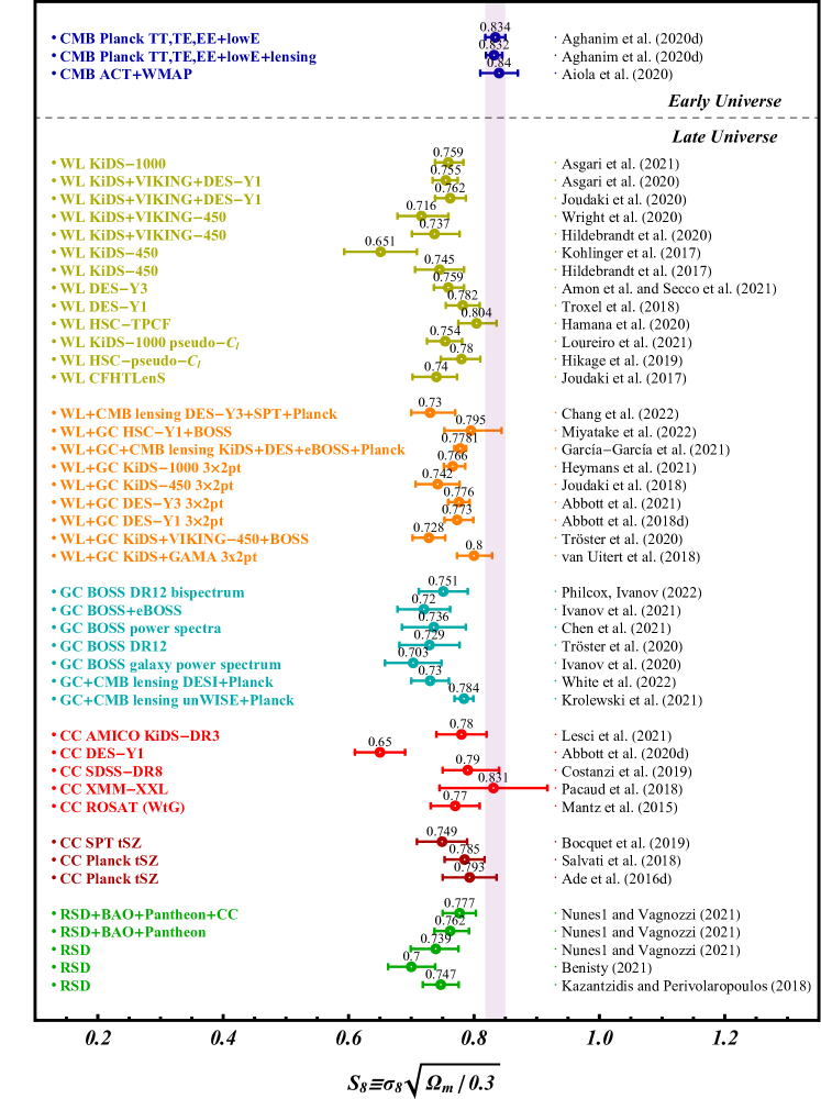
III.1.2 Theoretical models
Non-gravitational mechanisms can address the tension (see Ishak, 2019, for a review). Such mechanisms include the following:
-
•
Dynamical dark energy models (Roy et al., 2022; Linder, 2003; Cooray and Huterer, 1999; Efstathiou, 1999; Astier, 2001; Chevallier and Polarski, 2001; Weller and Albrecht, 2002; Feng et al., 2006; Nesseris and Perivolaropoulos, 2005; Jassal et al., 2005; Barboza and Alcaniz, 2008; Yang et al., 2017b; Melia, 2017; Yang et al., 2018d; Pan et al., 2018; Rezaei et al., 2017; Joudaki et al., 2017b; Du et al., 2019; Vagnozzi et al., 2018; Zhao et al., 2017a; Lambiase et al., 2019; Ooba et al., 2019; Yang et al., 2019d; Benisty and Staicova, 2021; D’Amico et al., 2021a) and running vacuum models (Solà et al., 2015, 2017a; Gómez-Valent and Solà, 2017; Gómez-Valent and Solà Peracaula, 2018; Wang et al., 2018; Colgáin et al., 2021; Solà Peracaula et al., 2021; Beltrán Jiménez et al., 2021), which modify the cosmological background to a form different from CDM (see Subsection II.2.1). This modification may involve the presence of dynamical dark energy dominant at late cosmological times or at times before recombination.
-
•
Interacting dark energy models, which modify the equation for the evolution of linear matter fluctuations as well as the cosmological background (Pourtsidou and Tram, 2016; An et al., 2018; Barros et al., 2019; Camera et al., 2019) as discussed in Subsection II.2.2. This class of models can address the structure growth tension between the values inferred from the CMB and the WL measurements.
-
•
Effects of massive neutrinos (Marulli et al., 2011; Battye and Moss, 2014; Costanzi et al., 2014; Joudaki et al., 2017b; Zennaro et al., 2018; Poulin et al., 2018a; Diaz Rivero et al., 2019; Biswas et al., 2019) which are relativistic at early times and contribute to radiation while at late times they become non-relativistic but with significant velocities (hot dark matter) (see Lesgourgues and Pastor, 2006; Wong, 2011; Lesgourgues and Pastor, 2012, 2014, for a review). The change of radiation to hot dark matter affects the Hubble expansion. Simultaneously the residual streaming velocities are still large enough at late times to slow down the growth of structure (Bond et al., 1980). This effect of massive neutrinos slows down the growth as required by the RSD data and relieves the tension coming from WL data (Diaz Rivero et al., 2019).
-
•
Primordial magnetic fields (Jedamzik and Saveliev, 2019; Banerjee and Jedamzik, 2004) (see Durrer and Neronov, 2013; Subramanian, 2016; Vachaspati, 2021, for a review) induce additional mildly non-linear, small-scale baryon inhomogeneities present in the plasma before recombination. The required field results in a reduction of the sound horizon scale at recombination and has the potential to resolve both the and tension (Jedamzik and Pogosian, 2020; Rashkovetskyi et al., 2021; Thiele et al., 2021).
-
•
Non-thermal dark radiation (Das et al., 2021b) seems to help alleviate the tension to a great extent. However, the inclusion of BAO data reduces significantly the quality of fit of this model.
In addition to these non-gravitational mechanisms discussed above that can slow down growth at low redshifts a possible interesting new fundamental physics approach can also reduce the tension. Such an approach is most likely to affect three basic observable parameters: the Hubble parameter (with the dark energy equation of state parameter), as well as the effective Newton constants for growth of perturbations
| (107) |
and lensing
| (108) |
where is the locally measured value of the Newton’s constant. According to CDM , , .
The Bardeen potentials (Bardeen, 1980) (the Newtonian potential and the spatial curvature potential ) appear in the scalar perturbed Friedmann-Lemaître-Robertson-Walker (FLRW) metric in the conformal Newtonian gauge (Mukhanov et al., 1992; Ma and Bertschinger, 1995; Esposito-Farese and Polarski, 2001)
| (109) |
The LSS probes are sensitive to the Bardeen potentials and . In particular the WL probe is sensitive to . The galaxy clustering arises from the gravitational attraction of matter and is sensitive only to the potential . The RSD probe is sensitive to the rate of growth of matter density perturbations (see Eq. (103)) and provides measurements of (see Eq. (106)) that depends on the potential .
At linear level, in modified gravity models, using the perturbed metric Eq. (109) and the gravitational field equations the following phenomenological equations in Fourier space emerge for the scalar perturbation potentials defining the functions and on subhorizon scales (i.e. )
| (110) |
| (111) |
where is the matter density of the background, the comoving matter density contrast defined as which is gauge-invariant (Pogosian et al., 2010), is the equation-of-state parameter and is the irrotational component of the peculiar velocity (Boisseau et al., 2000).
Using the gravitational slip parameter (or anisotropic stress parameter) which describes the possible inequality (Pogosian and Silvestri, 2008; Jain and Khoury, 2010) of the two Bardeen potentials that may occur in modified gravity theories
| (112) |
the two LSS parameters and are related via
| (113) |
The the Hubble parameter is usually parametrized as wCDM
| (114) |
while the two LSS parameters and do not have a commonly accepted parametrization. A model and scale independent parametrization for and which reduce to the GR value at early times and at the present time as indicated by solar system (ignoring possible screening effects) and BBN constraints ( and for and for ) (Muller et al., 2008; Pitjeva and Pitjev, 2013; Gannouji et al., 2006) is of the form (Nesseris and Perivolaropoulos, 2007; Nesseris et al., 2017; Kazantzidis and Perivolaropoulos, 2018; Skara and Perivolaropoulos, 2020)
| (115) |
| (116) |
where and are parameters to be fit and and are integer parameters with and .
Alternatively, a rapid transition parametrization is of the form (Alestas et al., 2021b; Marra and Perivolaropoulos, 2021)
| (117) |
| (118) |
where is the Heaviside step function, is a transition redshift, and correspond to and and correspond to .
Various studies utilize modified gravity theories including Teleparallel theories of gravity474747Many authors have studied the extensions of the Teleparallel gravity such as the scalar-torsion theories of gravity (Geng et al., 2012, 2011; Gonzalez-Espinoza et al., 2021; Paliathanasis, 2021; Skugoreva et al., 2015; Kofinas et al., 2015; Leon et al., 2022) and the Teleparallel Horndeski theories (Dialektopoulos et al., 2021; Bernardo et al., 2021; Bahamonde et al., 2021a, 2020, 2019). (D’Agostino and Luongo, 2018; Gonzalez-Espinoza et al., 2018) (see Bahamonde et al., 2021b, for a review), Horndeski theories (Kennedy et al., 2018; Linder, 2018) or theories beyond Horndeski (D’Amico et al., 2017) to reduce the effective Newton’s constant at low redshifts and slow down growth at low redshifts. The above parametrizations can be realized in the context of physical models based on the above theories.
III.2 CMB anisotropy anomalies
There is a wide range of other less discussed no-standard signals and statistical anomalies of the large angle fluctuations in the CMB (Rassat et al., 2014) with a typical to significance. As mentioned a main assumption of the CDM model is that the fluctuations are Gaussian and statistically homogeneous and isotropic. Diverse anomalies have been noticed in the CMB at large angular scales by the space missions Cosmic Background Explorer (COBE) (Mather et al., 1990), Wilkinson Microwave Anisotropy Probe (WMAP) (Bennett et al., 2003b) and Planck satellite (Adam et al., 2016), which appear to violate this assumption (see Schwarz et al., 2016; Akrami et al., 2020b, for a review). Perivolaropoulos (2014) presents possible explanations of the observed CMB anomalies and Cayuso and Johnson (2020) explore the kinetic and the polarized Sunyaev-Zel’dovich effects as potential probes of physical models of these anomalies.
In what follows we discuss some of these signals. Note that some of these may not be independent484848The covariance of CMB anomalies in the standard CDM model has been studied by Muir et al. (2018). This study focusing on the correlation of observed anomalies (i.e. the relationship or connection between all of them) examines the independence of large-angle CMB feature quantities.. Some of these signals have been attributed to the look-elsewhere effect. Based on this effect any large dataset will have a small number of peculiar features when there is a careful search for such features. However, this argument may not be applicable when the considered statistics are simple and generic as are most of the signals discussed below (see Bayer and Seljak, 2020; Peiris, 2014; Gross and Vitells, 2010, for a detailed discussion).
III.2.1 Hints for a closed Universe (CMB vs BAO)
The Universe under the assumption of the cosmological principle is described by the Friedmann-Lemaître-Roberson-Walker (FLRW) metric
| (119) |
where characterizes the constant spatial curvature of the spatial slices with corresponding to open hyperbolic space (negative spatial curvature), flat Euclidean space (zero spatial curvature), and closed hyperspherical space (positive spatial curvature) respectively. The curvature density parameter is defined as so that a closed Universe corresponds to and an open Universe to . This parameter plays a crucial role in determining the evolution of the Universe, and is closely related with the early Universe physics.
The Planck temperature and polarization data (Aghanim et al., 2020e) show a preference () for a closed Universe () in the context of CDM. In particular using these data from Planck the curvature density parameter was constrained to be at C.L (Aghanim et al., 2020e, d). This anomaly may be connected with other asymmetries of the CMB anisotropy spectrum discussed below. The preference for closed universe however disappears when the CMB data are combined with the BAO data. Di Valentino et al. (2021h, 2019b); Handley (2019) pointed out that Planck+BAO can give a biased result because Planck and BAO are in disagreement at more than . Combining Planck18 data with recent BAO measurements the curvature density parameter was estimated to be (Di Valentino et al., 2021h, 2019b; Handley, 2019) in agreement with a spatially flat Universe. Using the full-shape galaxy power spectrum measurements , Vagnozzi et al. (2021a) has also confirmed that the Planck data are in tension with both the full-shape power spectrum and BAO with respect to . The recent study by Efstathiou and Gratton (2020) confirms the tension between Planck and BAO data in the context of cosmic curvature. Efstathiou and Gratton (2020) used a new statistical analysis (the alternative Planck CamSpec likelihood TTTEEE instead of Plik as discussed in Efstathiou and Gratton (2019)) to show that Planck favors a closed Universe at more than CL. However, Planck+BAO was again found to be in agreement with a spatially flat Universe with thus confirming previous studies by Di Valentino et al. (2019b); Handley (2019) .
In an effort to further investigate this tension between Planck and BAO data, the analysis of Vagnozzi et al. (2021b) combined Planck18 CMB temperature and polarization data with cosmic chronometer measurements and was lead to confirm that the Universe is consistent with spatial flatness to () level.
III.2.2 Anomalously strong ISW effect
The decay of cosmological large-scale gravitational potential causes the integrated Sachs-Wolfe (ISW) effect (Sachs and Wolfe, 1967) which imprints tiny secondary anisotropies to the primary fluctuations of the CMB and is a complementary probe of dark energy (Kofman and Starobinsky, 1985; Fosalba and Gaztanaga, 2004; Giannantonio et al., 2008; Kable et al., 2021). Using a stacking technique in the CMB data (see Marcos-Caballero et al., 2016; Ade et al., 2016c, for a detailed discussion) anomalously strong integrated Sachs–Wolfe (ISW) signal () has been detected for supervoids and superclusters on scales larger than (Granett et al., 2008a, b). This stronger than expected within standard CDM signal of the ISW effect first emphasised in Hunt and Sarkar (2010) has been studied by Nadathur et al. (2012); Flender et al. (2013); Ilic et al. (2013); Cai et al. (2017c); Kovács et al. (2022); Kovács (2018); Kovács et al. (2019); Dong et al. (2020).
In particular the analysis by Kovács et al. (2019) for DES data alone found an excess ISW imprinted profile with amplitude (where corresponds to the CDM prediction). Also a combination with independent BOSS data leads to . This is in tension with CDM cosmology.
The average expansion rate approximation (AvERA) inhomogeneous cosmological simulation (Rácz et al., 2017) uses the separate Universe conjecture to calculates the spatial average of the expansion rate of local mini-Universes predicts. It indicates under the inhomogeneity assumption, about times higher ISW effect than CDM depending on the index of the spherical power spectrum (Beck et al., 2018). Thus large scale spatial inhomogeneities could provide an explanation to this ISW excess signal. Giannantonio et al. (2012) use angular cross-correlation techniques and combines several tracer catalogues to report .
Vagnozzi (2021) investigated the early Integrated Sachs-Wolfe (eISW) effect (see e.g. Bowen et al., 2002; Galli et al., 2010) which is assumed to occur soon after recombination (), due to the presence of a non-negligible radiation. Constraints were thus imposed on the parameter introduced by Hou et al. (2013). Using Planck CMB data, this parameter was constrained to , in perfect agreement with CDM. Note that in previous studies the parameter was constrained to using data from WMAP7+SPT (Hou et al., 2013), to from the Planck 2015 data release (Cabass et al., 2015), and to from the Planck 2018 temperature data alone (Kable et al., 2020).
In general the reported amplitude varies in the literature depending on the dataset and the assumptions of the analysis. Further investigation of this issue is needed.
III.2.3 CMB cold spot
The cold (blue) spot was first found in WMAP 1-year temperature data by Vielva et al. (2004) and was confirmed in Planck data (Ade et al., 2014b, 2016c; Akrami et al., 2020b) in the southern hemisphere at the galactic longitude and latitude . It is a statistical anomaly of the large-angle fluctuations in the CMB indicating non-Gaussian features. This inconsistency with Gaussian simulations has a p-value of .
The cold spot is an unusually large region of low temperature with the mean temperature decrement and is not consistent with the prediction of gaussianity of the standard CDM model (Cruz et al., 2005, 2006, 2007).
Zhang and Huterer (2010); Nadathur et al. (2014); Kovács (2018) pointed out that the anomalous nature of the cold spot corresponds to a rather cold area with an angular radius in the sky of about from the centre surrounded by a hot ring.
Possible approaches for the explanation of the Cold Spot include: non-Gaussian feature due to a large statistical fluctuation (Vielva et al., 2004), an artifact of inflation (Cruz et al., 2005), the foreground (Cruz et al., 2006; Hansen et al., 2012), multiple voids (Naidoo et al., 2016), the imprint of a supervoid (about radius completely empty void at ) through the ISW effect (Inoue and Silk, 2006, 2007; Rudnick et al., 2007; Granett et al., 2008a), the axis of rotation of the Universe (Jaffe et al., 2005), cosmic texture (Cruz et al., 2005; Zhao, 2013), adiabatic perturbation on the last scattering surface (Valkenburg, 2012) (see Cruz et al., 2009; Vielva, 2010, for a review).
III.2.4 Cosmic hemispherical power asymmetry
The cosmic hemispherical power asymmetry (or dipolar asymmetry) is a directional dependency of the CMB angular power spectrum (Eriksen et al., 2004; Hansen et al., 2004; Eriksen et al., 2007; Paci et al., 2010). The continuous dipolar modulation of hemispherical power asymmetry corresponds to a hemispherical temperature variance asymmetry (signal in the CMB temperature field) (Eriksen et al., 2004; Hansen et al., 2004; Monteserin et al., 2008; Hoftuft et al., 2009; Akrami et al., 2014; Bernui et al., 2014; Ade et al., 2016c; Akrami et al., 2020b; O’Dwyer et al., 2019).
The dipolar modulated/observed CMB temperature fluctuation in the direction which appears to extend to can be expressed as (Gordon, 2007; Bennett et al., 2011; Akrami et al., 2014)494949Note that the hemispherical dipole is distinct from the usual CMB dipole. In the former case the power spectrum is assumed modulated discontinuously across a circle on the sky and in the second the actual temperature map has a component modulated by a smooth cosine function across the sky (Bennett et al., 2011).
| (120) |
where is a statistically unmodulated/isotropic temperature fluctuation, denotes the amplitude of dipolar modulation and corresponds to the dipolar modulation between the line-of-sight (LOS) of the observer (with unit vector ) and the preferred dipolar direction (with unit vector ). The amplitude of dipolar modulation is large at large angular scales (), small at small angular scales and vanishes by a multipole moment of (Ade et al., 2014b, 2016c; Akrami et al., 2020b). The scale dependence of the hemispherical power asymmetry was suggested by Erickcek et al. (2008b); Liddle and Cortês (2013); Lyth (2015); Wang et al. (2016b); Mukherjee and Souradeep (2016); Yang et al. (2017a); Byrnes et al. (2016b, c, a); Ashoorioon and Koivisto (2016); Jazayeri et al. (2017) and was investigated by Shiraishi et al. (2016); Li et al. (2019a).
According to the hemispherical asymmetry nearly aligned with the Ecliptic, the temperature fluctuations are larger on one side of the CMB sky than on the other, resulting in an unexpected dipole configuration in the CMB power spectrum with an anomalously lower value of the variance in the northern sky compared to the southern sky (Ade et al., 2014b). The preferred direction for the asymmetry from the Planck18 data is in galactic coordinates and the amplitude is with statistically significant at the level (Akrami et al., 2020b). This amplitude is times higher than expected asymmetry due to cosmic variance () and it is inconsistent with isotropy () at the level. The hemispherical power asymmetry in CMB can be explained by assuming a superhorizon perturbation (Gordon et al., 2005; Gordon, 2007) or asymmetric initial states of the quantum perturbations (Ashoorioon and Koivisto, 2016).
III.2.5 Quadrupole-octopole alignment
The fluctuations in the standard CDM model are Gaussian and statistically isotopic. Thus in harmonic space the quadrupole () and octopole () harmonics are expected to have independent and random orientations and shapes. The quadrupole and octopole have been observed to be planar and unexpectedly aligned with each other (de Oliveira-Costa et al., 2004; Schwarz et al., 2004; Copi et al., 2006, 2007, 2010, 2015b). This implies a violation of statistical isotropy.
In particular in this low multipole moment anomaly the quadrupole and octopole planes are found to be mutually aligned with the direction of the cosmic dipole or CMB dipole (see Subsection III.3 and Table 3) and perpendicular to the Ecliptic (Schwarz et al., 2016).
In order to study this large-angle anomaly one can use the maximum angular momentum dispersion (de Oliveira-Costa et al., 2004)
| (121) |
where the CMB map is represented by a wave function
| (122) |
Here correspond to the spherical harmonic coefficients of the CMB map in a coordinate system with its -axis in the the -direction.
The preferred axis is the axis around which the angular momentum dispersion is maximized. The directions of the quadrupole and the octopole are (de Oliveira-Costa et al., 2004)
| (123) |
| (124) |
with
| (125) |
This unexpected alignment of the and directions has only a probability of happening.
An approach in the analysis of this large-angle anomaly may also involve the use the multipole vectors (Copi et al., 2004) (an alternative to the spherical harmonics) where each multipole order is represented by unit vectors i.e a dipole can be constructed by a vector, a quadrupole by the product of two vectors/dipoles, an octopole from three vectors/dipoles etc.
The alignment of low multipoles indicates the existence of a preferred direction in the CMB temperature anisotropy. Furthermore possible relation between the quadrupole-octopole alignment and the dipolar asymmetry has been investigated by Hoftuft et al. (2009); Gordon (2007). A negligible relation between these anomalies was reported. However the analysis by Marcos-Caballero and Martínez-González (2019) has shown that a particular dipolar modulation including the scale dependence may be connected with the quadrupole-octopole alignment.
III.2.6 Lack of large-angle CMB temperature correlations
There is a lack of large-angle CMB temperature correlations as first was observed by COBE satellite (Hinshaw et al., 1996) and was confirmed by the WMAP (Bennett et al., 2003a; Spergel et al., 2003) and Planck (Ade et al., 2016c; Akrami et al., 2020b) temperature maps in the range to . This is in tension with the CDM prediction.
This anomaly is directly connected to the temperature two-point angular correlation function of the CMB at large angular scale () which is unexpectedly close to zero (Copi et al., 2009, 2010, 2015a). In angular space the two-point angular correlation function is defined as
| (126) |
where the average is over all pairs of directions with , are the Legendre polynomials and is the angular power spectrum
| (127) |
with the spherical harmonic coefficients of the temperature fluctuations.
The simplest and most useful statistic is first introduced in the WMAP first-year release (Spergel et al., 2003) in order to measure the deviation of the angular correlation function from zero at angular scales . It is defined as
| (128) |
with and .
A number of alternative statistics have been proposed in the literature (Hajian, 2007; Efstathiou et al., 2010; Gruppuso, 2014; Akrami et al., 2020b). For example a generalization of the statistic suggested by Copi et al. (2013). This statistic known as uses the two-point angular correlation function between fluctuations in the temperature and the Stokes parameter505050The Stokes parameters Q and U (for the Stokes parameters formalism see Jackson, 1998) are used to describe the state of CMB polarization (e.g. Zaldarriaga and Seljak, 1997; Dodelson, 2003). These parameters are directly related to the E and B modes (Kamionkowski et al., 1997; Lewis et al., 2002; Bunn et al., 2003). The polarization amplitude is given by . , , which can be expressed in terms of the two-point angular power spectrum, (with the gradient mode of polarization). The significance of a test statistic can be quantified by using the p-value515151The probability value or p-value is the probability of measuring a test statistic equal to or more extreme as the observed one, considering that the null hypothesis is correct (Ade et al., 2014b). It provides the lower value of significance at which the model would be ruled out. A low p-value means that there is strong indication of new physics beyond the null hypothesis., suggested by Ade et al. (2014b).
No sufficient explanation has yet been suggested for this large-angle anomaly. Copi et al. (2016) study the ISW effect, Aurich et al. (2021); Bernui et al. (2018) explore a non-trivial spatial topology of the Universe and Pranav et al. (2019) study the topology of the Planck CMB temperature fluctuations in order to find a possible explanation to the suppression of large-angle CMB temperature correlations. Also the low observed power in the quadrupole is a potential explanation for the lack of correlation in the temperature maps. Copi et al. (2009) argue that there is a cancellation between the combined contributions of with multipoles and the contributions of with multipoles .
III.2.7 Anomaly on super-horizon scales
Pranav (2021) analysed the topological characteristics of the CMB temperature fluctuation. Using mathematical investigations on persistent homology to describe the cosmic mass distribution and performing experiments on Planck 2020 data release 4 (DR4) (based on the NPIPE data processing pipeline Akrami et al. 2020d), Pranav (2021) claimed a detection of an anomalous topological signature in the Planck CMB maps indicating non-Gaussian fluctuations. In particular Pranav (2021) reports an anomaly in the behavior of the loops (a deviation in the number of loops) in the observed sky compared to the analysis of the redshift evolution of structure on simulations when the CDM model is considered.
III.2.8 The lensing anomaly
The recent Planck release by Aghanim et al. (2020e) has confirmed the higher compared to that expected in the standard CDM model, anomalous, lensing contribution in the CMB power spectra which is quantified by the phenomenological parameter, (Calabrese et al., 2008; Zaldarriaga and Seljak, 1998). This weak lensing parameter rescales the lensing potential power spectrum as525252Note that this is not the usual but it is the additional contribution due to lensing.
| (129) |
where corresponds to unlensed while is the expected lensed result (Calabrese et al., 2008) measuring the lensing effect in the CMB temperature power spectrum.
Since the main impacts of lensing on the CMB temperature power spectrum are to add power at small scales and to smooth the structure of the acoustic peaks and troughs (the peaks are reduced slightly, and the troughs between them filled in) (Lewis and Challinor, 2006; Ade et al., 2016b) the adding of parameter changes the amount of smoothing of the CMB primary spectra peaks and troughs. A higher lensing amplitude () than predicted in the flat CDM cosmology () by roughly (at the level of ) has been found in the temperature power spectra by the Planck team (Aghanim et al., 2020e).
It should be noted that the oscillatory residuals between the Planck temperature power spectra and the best-fit CDM model in the multipole range are in opposite phase compared to the CMB and thus phenomenologically similar to the effects of gravitational lensing (Aghanim et al., 2017; Motloch and Hu, 2020).
A plausible explanation of the anomalous lensing amplitude is a positive curvature (closed Universe) which was investigated by Di Valentino et al. (2021h, 2019b); Handley (2019). Other possible sources which explain the lensing anomaly by mimicking a lensing effect are: a component of cold dark matter isocurvature (CDI) perturbation with a blue tilt (see Akrami et al., 2020c, for a detailed discussion) and oscillations in the primordial power spectrum which have the same frequency but opposite phase with the acoustic peaks (Aghanim et al., 2020e). All these effects are degenerate with the smoothing effect of lensing.
Furthermore, the modified gravity models could be candidates for a solution of the lensing anomaly (Ade et al., 2016e; Di Valentino et al., 2016a; Moshafi et al., 2021; Di Valentino et al., 2020a). In particular the hints for (where the current value of parameter which modifies the equation for the lensing potential i.e. Eq. (110)) are directly connected to the lensing anomaly as characterized by (Di Valentino et al., 2016a, 2020a).
III.2.9 High-low l consistency
Addison et al. (2016) pointed out that there are internal inconsistencies in the Planck TT power spectrum. The CDM parameter values derived by the high part of the CMB anisotropy spectrum () are in tension with the corresponding values of these parameters derived from the low part of the spectrum (). For example the low multipoles predict a lower value of the cold dark matter density parameter than the high multipoles, with discrepancy at (Addison et al., 2016). In addition it has been shown that the value of predicted by Planck from , , disagrees with the value predicted by Planck from , at the level. Thus it is found that the value of depends on the CMB -range examined.
III.2.10 The preference for odd parity correlations
There is an anomalous power excess (deficit) of odd (even) multipoles in the CMB anisotropy spectrum on the largest angular scales (), (Land and Magueijo, 2005; Kim and Naselsky, 2010b, a, 2011; Gruppuso et al., 2011, 2018; Akrami et al., 2020b). A map consisting of odd (even) multipoles possesses odd (even) parity thus this effect may be considered as power (spectrum) asymmetry between even and odd parity map which is known as parity asymmetry.
In order to compare even and odd multipoles Kim and Naselsky (2010a) consider the parity asymmetry statistic defined as the ratio of quantities and which represent the mean power in even and odd only multipoles respectively for the range
| (130) |
A different statistic to quantify the parity asymmetry has been proposed by Aluri and Jain (2012).
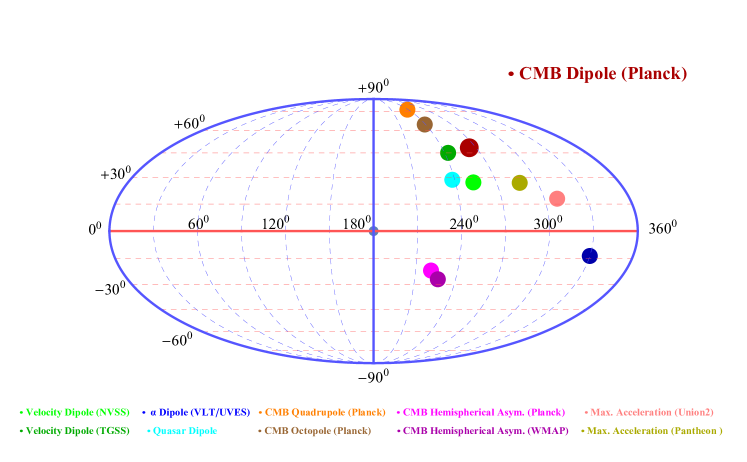
III.3 Cosmic dipoles
There have been studies pointing out the presence of signals which indicate the violation of the cosmological principle. A physical mechanism producing such violation on Hubble scales is studied by Bueno Sanchez and Perivolaropoulos (2011). Various other possible mechanisms have been suggested to explain the observed violations of statistical isotropy e.g. superhorizon perturbations which introduce a preferred direction in our Universe (Gordon et al., 2005; Erickcek et al., 2008a) (see also Perivolaropoulos, 2014, for a review). The dipole amplitudes and the directions (galactic coordinates) from the different cosmological observations described below are shown in Fig. 22 and along with the corresponding references in Table 3.
| Observations | Amplitude | Refs. | |||||
|---|---|---|---|---|---|---|---|
| CMB Dipole (Planck) | (Aghanim et al., 2020b, c) | ||||||
| Velocity Radio Dipole (TGSS) | (Bengaly et al., 2018) | ||||||
| Velocity Radio Dipole (NVSS) | (Bengaly et al., 2018) | ||||||
| Velocity Radio Dipole (NVSS) | (Colin et al., 2017) | ||||||
| Velocity Radio Dipole (NVSS) | (Tiwari and Nusser, 2016) | ||||||
| Quasar Dipole | (Secrest et al., 2021) | ||||||
| Dipole (VLT/UVES) | (King et al., 2012) | ||||||
| CMB Quadrupole (Planck SMICA535353Spectral Matching Independent Component Analysis (SMICA) is a method to extract the CMB component (Akrami et al., 2020a) described in Cardoso et al. (2008).) | (Ade et al., 2014b) | ||||||
| CMB Octopole (Planck SMICA) | (Ade et al., 2014b) | ||||||
| CMB Hemispher. Asym. (Planck) | (Akrami et al., 2020b) | ||||||
| CMB Hemispher. Asym. (WMAP) | (Axelsson et al., 2013) | ||||||
| Maximum Acceleration (Pantheon) | (Kazantzidis and Perivolaropoulos, 2020) | ||||||
| Maximum Acceleration (Union2) | (Antoniou and Perivolaropoulos, 2010) |
The physical origin of these dipoles is described in the following subsections.
III.3.1 Velocity radio dipole
A large scale velocity flow dipole545454For peculiar velocities as variation of the Hubble expansion produced by nearby nonlinear structures see in Wiltshire et al. (2013) and for dipole anisotropy in radio source count, see in Bengaly et al. (2018). was pointed out in Watkins et al. (2009); Kashlinsky et al. (2009). The dipole moment of the peculiar velocity field (dipole bulk flow) which is a sensitive probe of the amplitude and growth rate of fluctuations on large scales (Koda et al., 2014) was investigated by Watkins et al. (2009); Feldman et al. (2010); Kashlinsky et al. (2009, 2010); Nusser and Davis (2011); Ma and Scott (2013); Turnbull et al. (2012); Kashlinsky et al. (2012); Hong et al. (2014). In many cases the results are controversial and there is a debate in the literature on the consistency with the CDM model.
A recent detailed analysis has indicated that ’tilted observers’ within the bulk flow can be misled into inferring acceleration (Tsagas, 2011; Tsagas and Kadiltzoglou, 2015; Tsagas et al., 2021) (see also Asvesta et al., 2022, for observational constraints of the deceleration parameter in a tilted universe).
Colin et al. (2019) use SnIa JLA data to demonstrate that the indications for cosmic acceleration found in the SnIa data disappears if a bulk flow induced anisotropy is allowed in the SnIa data. Thus, a bulk flow dipole (at ) aligned with the local bulk flow is identified while any monopole (which can be attributed to ) is consistent with zero (at ).555555A recent model independent analysis of SnIa data (Pantheon) data Arjona and Nesseris (2020) implementing machine learning has confirmed a detection of the accelerated expansion even though that analysis did not allow for anisotropic dipole effects.
It is usually assumed that our local (solar system) peculiar motion with respect to the CMB rest frame produces the CMB dipole anisotropy () (Kogut et al., 1993; Fixsen et al., 1996) (also known as solar dipole Aghanim et al., 2016, 2020c). In the standard model, this implies that the LSS distribution should have a similar kinematic dipole known as the velocity dipole or radio dipole which arises from the Doppler boosting of the CMB monopole and from special relativistic aberration effects (Itoh et al., 2010).
In order to describe the origin of this dipole, a population of sources with power-law spectra depending on frequency is usually assumed
| (131) |
where is the flux density and 565656The individual spectral index should not be confused with the fine-structure constant . is an individual spectral index with typically assumed value (Bacon et al., 2020). The integral source counts per unit solid angle above some limiting flux density can be approximated by a power law
| (132) |
where and can be different for each survey. An observer moving with velocity with respect to the frame in which these sources are isotropically distributed sees a dipole anisotropy over the sky with amplitude (Ellis and Baldwin, 1984)
| (133) |
According to the most recent measurements the inferred velocity of the Sun relative to the CMB rest frame is (Aghanim et al., 2020b, c)
| (134) |
| (135) |
along the direction with galactic longitude and latitude or , (Aghanim et al., 2020b, c).
The CMB rest frame is conventionally taken to correspond to the standard of cosmic rest frame and is assumed to be statistically homogeneous and isotropic in the context of the FLRW model. In this rest frame the Hubble flow should be most uniform (minimum Hubble variation frame) and the comoving observers should not see a kinematic dipole. However it has been observed (Wiltshire et al., 2013; McKay and Wiltshire, 2016) that the dipole structure of the velocity field is less in the reference frame of the Local Group of galaxies than in the CMB frame. This persistence of the dipole structure of the velocity flow in the CMB frame at large distances is not unexpected if we are located in an underdensity (Kraljic and Sarkar, 2016).
According to the standard model if the Universe is isotropic our velocity with respect to the CMB rest frame and our velocity relative to the LSS should be identical. However, as was first noted by Singal (2011), while the direction of the radio dipole is consistent with that of the CMB, the velocity of our local motion obtained from the radio dipole exceeds that obtained from the CMB dipole. Radio continuum surveys which sample the Universe at intermediate redshifts () have been used as an excellent probe to large scale isotropy and a discrepancy between the predicted and measured amplitudes of the velocity have been revealed (Gibelyou and Huterer, 2012; Rubart and Schwarz, 2013; Tiwari et al., 2014; Tiwari and Nusser, 2016; Colin et al., 2017; Bengaly et al., 2018). In particular the analysis by Bengaly et al. (2018) has shown that the radio dipole using the sky distribution of radio sources from the NRAO VLA Sky Survey (NVSS) dataset (Condon et al., 1998) and TIFR GMRT Sky Survey (TGSS) dataset (Bengaly et al., 2018; Intema et al., 2017; Singal, 2019a) is and times larger than predicted by the mock realisations within the context of CDM cosmology respectively. The above observed discrepancy between the radio and CMB dipoles has been confirmed by independent groups and could imply the existence of an anisotropic Universe.
Possible explanations of the violation of statistical isotropy are: systematics due to the incomplete sky coverage of the radio continuum surveys (Blake and Wall, 2002; Gibelyou and Huterer, 2012; Tiwari and Nusser, 2016), intrinsic dipole in the local LSS (Fernández-Cobos et al., 2014), nearby nonlinear structures of voids and walls and filaments (Wiltshire et al., 2013), remnant of the pre-inflationary Universe (Turner, 1991) and superhorizon perturbation (Ghosh, 2014; Das et al., 2021a).
III.3.2 Quasar dipole
The distribution of quasars across the sky may provide independent probe of the cosmological principle (Singal, 2019b). As previously discussed there is an expected anisotropy related to the CMB dipole anisotropy (about 1 part in 1000) due to our motion with respect to the CMB rest frame.
Secrest et al. (2021) used mid-infrared data from the Wide-field Infrared Survey Explorer (WISE) (Wright et al., 2010) to create reliable AGN/quasar catalogs and a custom quasar sample from the new CatWISE2020 data release (Eisenhardt et al., 2020). It was shown that there is a statistically significant dipole in the density of distant quasars with direction which is away from the direction of the CMB dipole. Its amplitude was found to be , times larger than predicted, with statistical significance at the level (or with a p-value of ) for a normal distribution. This result is in conflict with the cosmological principle.
III.3.3 Fine structure constant dipole
In the past years there has been interest in the possibility of the variation of the fine structure constant (where , , , and are the electron charge, the vacuum permittivity, the reduced Planck’s constant, and the speed of light) (Murphy et al., 2003; Webb et al., 2011; Molaro et al., 2013; Berengut et al., 2013; Webb et al., 2014; Evans et al., 2014; Bainbridge et al., 2017; Hu et al., 2019; Milaković et al., 2020; Lee et al., 2021) (for review of varying fine structure constant, see Martins, 2017).
The analysis by King et al. (2012); Webb et al. (2011) uses the “many multiplet” (MM) method (Webb et al., 1999; Dzuba et al., 1999; Webb et al., 2001; Murphy et al., 2001) to analyze quasar absorption line spectra obtained using the Ultraviolet and Visual Echelle Spectrograph (UVES) (Dekker et al., 2000) on the Very Large Telescope (VLT). It indicates both the violation of the cosmological principle and the spatial variation of the fine structure constant which is approximated as a spatial dipole with direction and amplitude , preferred over a simple monopole model with significance at the (for possible systematics in this analysis, see Cameron and Pettitt, 2012; Kanekar et al., 2012; Levshakov et al., 2012).
The variation of across the sky was shown to be well fit by an angular dipole model of the form (King et al., 2012)
| (136) |
where is the present local value, is the angle with respect to the dipole direction, is the angular amplitude of the dipole term and is a monopole term.
It is worth to note that the analysis by Martins and Pinho (2017) suggests that there are no robust indications of time or space variations of . However recent measurements of quasar absorption-line spectra indicate a spatially dependent value of fine structure constant at a significance level over a simple monopole (no-variation) model (Dumont and Webb, 2017; Wilczynska et al., 2020). In addition, it is found that the fine structure constant dipole is anomalously aligned with other dipoles and the preferred direction in is correlated with the one in the distribution of SNIa (Mariano and Perivolaropoulos, 2012, 2013).
III.4 BAO curiosities
As mentioned above (see Subsection II.1.2) the BAO measurements can be classified in two classes: galaxy BAO and Ly BAO (with Ly auto-correlation function and Ly-quasar cross-correlation function). A discrepancy between the BAO peak position in the Ly at an effective redshift of and the CMB predictions from Planck/CDM cosmological model has been found (Font-Ribera et al., 2014; Aubourg et al., 2015; du Mas des Bourboux et al., 2017).
For example, Aubourg et al. (2015) use the Ly auto-correlation function and the Ly-quasar cross-correlation function to report the measurements of the BAO scale in the line-of-sight direction
| (137) |
and in the transverse direction
| (138) |
where is the Hubble distance and is the comoving angular diameter distance. These values are in tension with CMB predictions and by Planck 2015 flat CDM cosmology (Ade et al., 2016a).
The galaxy BAO peak position in the matter correlation function (see Eq. (24) and Fig. 7) and the measurements and were found to be consistent with CMB predictions. This discrepancy between galaxy and Ly BAO constitutes the BAO anomaly which has been investigated in Cuceu et al. (2019); Evslin (2017); Addison et al. (2018).
Using new Ly BAO measurements from the BOSS survey and from its extended version eBOSS in the SDSS DR the tension with CMB predictions was reduced to (Blomqvist et al., 2019; de Sainte Agathe et al., 2019) and from eBOSS in the SDSS DR to only (du Mas des Bourboux et al., 2020).
Evslin (2017) argues that this anomaly arises by cosmological effects at and the tension is caused by evolution of dark energy equation of state for redshift range .
III.5 Parity violating rotation of CMB linear polarization (Cosmic Birefringence)
In the standard model of elementary particles and fields, parity violation is observed only in the weak interaction sector (Lee and Yang, 1956; Wu et al., 1957). A certain class of quintessence models should generically generate such parity asymmetric physics (Carroll et al., 1990; Carroll, 1998). In particular a parity violating (nearly) massless axionlike scalar field (dark matter or dark energy) would rotate CMB polarisation angles of CMB photons as they travel from the last scattering surface () to the present by a non-zero angle (cosmic birefringence).
A Chern–Simons coupling between a time-dependent axionlike field and the electromagnetic tensor and its dual in the Lagrangian density (e.g. Ni, 1977; Turner and Widrow, 1988; Carroll et al., 1990)
| (139) |
induces a cosmic isotropic birefringence angle (e.g. Harari and Sikivie, 1992; Fujita et al., 2021a)
| (140) |
and produces a non-zero observed spectrum (Lue et al., 1999)
| (141) |
where is a Chern-Simons coupling constant which has mass-dimension , is the dual of the electromagnetic tensor of , and and are the times at present and last scattering surface, respectively.
Using a novel method developed in Minami et al. (2019); Minami (2020); Minami and Komatsu (2020b), a non-zero value of the isotropic cosmic birefringence ( C.L) was recently detected in the Planck18 polarization data at a statistical significance level by Minami and Komatsu (2020a). More recently, using the latest Planck public data release 4 (Akrami et al., 2020e) a birefringence angle of ( C.L) was reported by Diego-Palazuelos et al. (2022).
These recent evidences of the non zero value of birefringence poses a problem for standard CDM cosmology and indicates a hint of a new ingredient beyond this model.
An axion or an axion-like particle with a weak coupling to photon as a possible source of the cosmic birefringence was investigated by Fujita et al. (2021b) and a two-axion alignment model with periodic potential was investigated by Obata (2021). Takahashi and Yin (2021b) showed that if an ultralight axion coupled to photons forms domain walls due to inflationary fluctuations, the domain-wall network can explain the hint for isotropic cosmic birefringence found by Minami and Komatsu (2020a). This model predicts a testable peculiar anisotropic cosmic birefringence as well. In contrast to the approach of Fujita et al. (2021b), this scenario explains the birefringence with the photon anomalous coefficient of the axion-like particle . Furthermore, birefringence inducing axion-like particles could be candidates for an early dark energy resolution to the Hubble tension (Fujita et al., 2021b). Bianchini et al. (2020); Namikawa et al. (2020) study the anisotropic birefringence and constraints are derived. The axion field fluctuations over space and time generate anisotropic birefringence.
III.6 Small-scale curiosities
On small scales (on scales of hundreds of and below) the predictions of CDM model are in many cases inconsistent with observations (Kroupa et al., 2010; Weinberg et al., 2015; Nakama et al., 2017). In particular observations on galaxy scales indicate that the CDM model faces several problems in describing structures at small scales () (see Kroupa, 2012, 2015; Del Popolo and Le Delliou, 2017; Bullock and Boylan-Kolchin, 2017; Salucci, 2019, for a review). Alternative models that modify the nature of dark matter have been used to solve these problems e.g. warm (Bode et al., 2001; Abazajian, 2006; Viel et al., 2005; Schneider et al., 2014; Viel et al., 2013), fuzzy (Hu et al., 2000; Hui et al., 2017; Schive et al., 2014; Iršič et al., 2017), self-interacting (Carlson et al., 1992; Blennow et al., 2017; Garcia-Cely and Chu, 2017; Tulin and Yu, 2018) and meta-cold dark matter (Strigari et al., 2007) (see also de Martino et al., 2020, for a review). Other models which have the potential to provide a solution to these problems have been proposed by Foot and Vagnozzi (2015, 2016); Sawala et al. (2016); Schewtschenko et al. (2016); Vogelsberger et al. (2016); Archidiacono et al. (2017). In particular Foot and Vagnozzi (2015, 2016) argued that the existence of a dissipative hidden dark matter sector (dark matter coupled to a massless dark photon) can solve some of these problems (core-cusp, missing satellites, and plane of satellites problem).
These small scale signals include the following:
III.6.1 The core-cusp curiosity
The core-cusp curiosity (Moore, 1994; Flores and Primack, 1994; de Blok, 2010) (see also Cooke et al. 2022; Lelli 2022) refers to a discrepancy between the density of a dark matter halo profile of low-mass galaxies in N-body simulations (an important tool for evaluating the predictions of the CDM model) with (cusp profile)575757The well know Navarro–Frenk–White profile (Navarro et al., 1996b, 1997) is cusped with . (Navarro et al., 1997, 1996a; Moore et al., 1999b; Ferrero et al., 2012) and the astronomical observed profile with (core profile) (Moore, 1994; Davis et al., 1985; Navarro et al., 1997, 1996a; Flores and Primack, 1994; Battaglia et al., 2008; Walker and Penarrubia, 2011; Amorisco and Evans, 2012; Genina et al., 2017). McGaugh and de Blok (1998) probe this problem in low surface brightness galaxies.
III.6.2 The missing satellites problem (or dwarf galaxy problem)
The missing satellites problem (or dwarf galaxy problem) (Kauffmann et al., 1993; Klypin et al., 1999; Moore et al., 1999a; Bullock, 2010) refers to an over-abundance of the predicted number of halo substructures in detailed collisionless N-body simulations compared to the observed number of satellite galaxies in the Local Group. In particular the CDM model predicts orders of magnitude larger number of satellites () than the observed number of dwarf galaxies () (Mateo, 1998; Moore et al., 1999a).
III.6.3 The Too Big To Fail (TBTF) problem
The Too Big To Fail (TBTF) problem (Boylan-Kolchin et al., 2011, 2012; Garrison-Kimmel et al., 2014; Papastergis et al., 2015; Tollerud et al., 2014; Kaplinghat et al., 2019) refers to an inconsistency between the predicted mass of dark matter subhaloes in CDM theory and the observed central mass of brightest satellite galaxies in the Local Group (Garrison-Kimmel et al., 2014; Papastergis et al., 2015) (also in the MW Boylan-Kolchin et al. 2011, 2012 or in the Andromeda (M31) Tollerud et al. 2014).
In particular the CDM predicted central densities of the most massive dark matter subhalos are systematically larger than the inferred from kinematics of the brightest Local Group satellites (Read et al., 2006; Boylan-Kolchin et al., 2012; Garrison-Kimmel et al., 2014). An observed bright satellite is more likely to reside in subhalos with lower mass than is expected in a CDM model. The simulated massive dark matter subhalos ’failed’ to form a comparatively bright satellite galaxy.
This problem is possibly related to the missing satellites problem but it is a distinct problem which dependents on the internal structure of subhalos or the central shapes of density profiles of satellite halos (Garrison-Kimmel et al., 2014).
Alternative models that modify the nature of dark matter have been investigated to solve this problem: non-trivial dark matter physics (Lovell et al., 2017; Bozek et al., 2019), interaction between the dark matter and dark radiation components (Schewtschenko et al., 2016; Vogelsberger et al., 2016), self-interacting dark matter (Zavala et al., 2013; Vogelsberger et al., 2012) and fuzzy dark matter (Schive et al., 2014)
III.6.4 The problem of satellite planes
In the problem of satellite planes (Kroupa et al., 2005; Ibata et al., 2014; Conn et al., 2013; Pawlowski et al., 2014; Pawlowski, 2018) several satellite galaxies of the MW, of neighboring Andromeda galaxy (M31), and of Centaurus A (CenA) are part of thin plane that is approximately perpendicular to the Galactic disk. Moreover measurement of the motions of satellite galaxies has shown that their orbits appear to be correlated (Pawlowski et al., 2012; Ibata et al., 2013; Sohn et al., 2020). This flattened structure and coherent motions of satellite galaxy systems is in inconsistency with the prediction of the CDM model as inferred from simulations (Pawlowski, 2018). The simulations based on CDM cosmology indicate uncorrelated and close to isotropic satellite structures (Libeskind et al., 2005; Zentner et al., 2005). In these simulations the observed structure formations with spatial and kinematic coherence distribution are very rare with a probability (Pawlowski et al., 2014; Pawlowski, 2018).
III.6.5 The angular momentum catastrophe
The angular momentum catastrophe (van den Bosch et al., 2001) concerns a catastrophic angular momentum loss of gas during disk galaxies formation in Smooth Particle Hydrodynamics (SPH) (Monaghan, 1992) simulations. The formed disks in simulations according to the predictions of CDM have smaller scale lengths by a factor of compared with observed ones (Bullock et al., 2001). An axion dark matter model may resolve this discrepancy between the observed and predicted angular momentum distributions of baryons (ordinary cold dark matter) in the dwarf galaxies (Banik and Sikivie, 2013).
III.6.6 Baryonic Tully-Fisher Relation (BTFR)
Baryonic Tully-Fisher Relation (BTFR) (McGaugh, 2011; Lelli et al., 2016b). As mentioned above, the well known Tully-Fisher (TF) (Tully and Fisher, 1977) empirical relation connects the velocity of rotation of a spiral galaxy with its intrinsic luminosity while the Baryonic Tully-Fisher Relation (BTFR) (McGaugh et al., 2000; Verheijen, 2001; Gurovich et al., 2004) Eq. (46) is a scaling relation between the observed total baryonic mass (stars plus gas) of a spiral galaxy and its rotation velocity (see Subsection II.1.6). The problem for CDM model as inferred from simulations (e.g. Dutton, 2012) is that the BTFR leads to existence of a higher intrinsic scatter () and a lower slope () compared to the observed ( and ) (Lelli et al., 2016b). McGaugh (2012) suggests the Modified Newtonian Dynamics (MOND) (Milgrom, 1983) as a possible solution to this problem. However some simulations or semi-analytic approaches of galaxy formation within a CDM cosmological context can reproduce a realistic BTFR slope but not its small scatter (e.g. Sales et al., 2017; Di Cintio and Lelli, 2016; Geha et al., 2006; Santos-Santos et al., 2016).
III.6.7 The void phenomenon
The void phenomenon(Peebles, 2001) refers to the emptiness of voids (the number of small galaxies in the void). Cosmological N-body simulations in the context of CDM have established a clear prediction (Gottloeber et al., 2003) that many small dark matter haloes should reside in voids (Peebles, 2005, 2007). This is consistent with observations on large scales but is inconsistent with observations on small scales. In particular the local void contains much fewer galaxies than expected from CDM theory (Tikhonov and Klypin, 2009).
III.7 Age of the Universe
A lower limit can be set on the age of the Universe by the ages of the oldest stars (or oldest astrophysical objects) because on cosmological timescales they form shortly after the Big Bang. In the context of CDM cosmology, the standard theory (Haiman et al., 1996; Bromm et al., 2002; Abel et al., 2002; Bromm and Larson, 2004; Bromm, 2013) and cosmological numerical simulations (Yoshida et al., 2003; Hirano et al., 2015; Xu et al., 2016) predict that the first stars, the so-called population III (Pop III), formed in dark matter minihaloes of typical mass at redshifts (about million years after the Big Bang i.e. about around the end of the cosmic dark ages) (for models indicating late, , Pop III star formation, see Tornatore et al., 2007; Johnson, 2010).
The age of the Universe as obtained from local measurements using the ages of oldest observed stars (the so-called population II (Pop II)) in the MW appears to be larger and in some tension with the corresponding age of the Universe obtained using the CMB Planck data in the context of CDM (Verde et al., 2013).
The age of the Universe in the flat CDM model is an observable determined by the integral
| (142) |
where is the cosmic time corresponding to redshift . Thus the age of the Universe is .
For example the age of the MW Population II halo, metal deficient, high velocity subgiant HD- (also known as Methuselah star) is estimated to be by Bond et al. (2013) and using new sets of stellar models is estimated to be by VandenBerg et al. (2014). These estimates of the age of this star are slightly higher () than the age of Universe inferred by CMB Planck18 data (Aghanim et al., 2020e) but within the errors it does not conflict with this age.
Despite of the above indications the analysis by Jimenez et al. (2019) using new parallaxes from the Gaia space mission (Perryman et al., 2001; Prusti et al., 2016) in place of the older HST, reports a revision of the age of HD- to which is more compatible with the age inferred by Planck data. Also the analysis by Valcin et al. (2020) using populations of stars in globular clusters (very-low-metallicity stars) reports age of the Universe constrained to be larger than .
Clearly, Eq. (142) indicates that in a CDM Universe the quantities , and are related. Therefore the determination of the age of older objects based on local Universe observations provides a test of the current cosmological model and plays an important role in the studies of Hubble and spatial curvature tensions (Jimenez et al., 2019; Di Valentino et al., 2019b, 2021h; Wei and Melia, 2022).
III.8 The Lithium problem
It has long been known (since the early 80’s) that absorption lines in the photospheres of old, metal-poor (Population II) halo stars in the Milky Way’s halo indicate times less primordial abundance of lithium isotope compared to the prediction of the standard BBN theory (Cyburt et al., 2003; Asplund et al., 2006; Cyburt et al., 2008). The observed value of the lithium abundance585858Usually in the literature the abundance of lithium is expressed by where is the number density of atoms and is the solar hydrogen abundance. (Zyla et al., 2020) is smaller than the theoretically expected value (Pitrou et al., 2018) at a level . This constitutes the lithium problem (Fields, 2011). No such problem exists for the observed abundances of other light elements (or ), , and that are in broad quantitative agreement with BBN predictions + WMAP/Planck cosmic baryon density which is deduced by the CMB (Cyburt et al., 2016; Tanabashi et al., 2018).
A number of theoretical or experimental studies in the literature have attempted to address the lithium problem (e.g. Hammache et al., 2013; Pizzone et al., 2014; Yamazaki et al., 2014; Kusakabe et al., 2014; Poulin and Serpico, 2015; Sato et al., 2017a; Goudelis et al., 2016; Salvati et al., 2016; Hou et al., 2017; Coc and Vangioni, 2017; Mori and Kusakabe, 2019; Hayakawa et al., 2020; Ishikawa et al., 2020; Iliadis and Coc, 2020). For example the analysis by Clara and Martins (2020) shows that the variations in Nature’s fundamental constants on primordial nucleosynthesis provide a possible solution to the lithium problem. Specifically, they determined that if the value of the fine-structure constant at the primordial nucleosynthesis epoch was larger than the present one by ten parts per million of relative variation, the lithium problem could be resolved.
It was also proposed by Di Bari et al. (2013) that decaying dark matter into dark radiation in the early Universe can solve the long-standing lithium problem, leaving completely unaffected the abundance of other light elements. This mechanism was also proposed to alleviate the tension (see Subsection II.2.1) but is severely constrained by the Planck data (Anchordoqui, 2021).
Measurements of lithium (e.g. Sbordone et al., 2010; Melendez et al., 2010) may not be representative of the cosmological production mechanism (Spite et al., 2012; Iocco, 2012). It is thus possible that the solution to the lithium problem lies in the effects of stars in the lithium abundance. Therefore a precise knowledge of the stellar formation process and physics of stellar atmosphere is necessary to provide a fully satisfactory solution. Thus, possible solutions to this persistent problem can be classified into four categories (see Fields, 2011; Cyburt et al., 2016; Mathews et al., 2020, for a review):
-
•
Cosmological solutions (e.g. new theory beyond the standard BBN including variations of fundamental constants) (Franchino-Viñas and Mosquera, 2021; Clara and Martins, 2020; Larena et al., 2007; Kohri and Takayama, 2007; Berengut et al., 2010; Kawasaki and Kusakabe, 2011; Cheoun et al., 2011; Coc et al., 2007; Hou et al., 2017; Luo et al., 2019)
- •
- •
-
•
Extensions of the standard model (e.g. simultaneous imposition of photon cooling after BBN, X-particle decay and a primordial magnetic field (Yamazaki et al., 2014, 2017), destruction of 7Be due to the decay of a sterile neutrino (Salvati et al., 2016) and including new particles or interactions (Goudelis et al., 2016).
III.9 Quasars Hubble diagram
The quasar distances can be estimated from their X-ray (coronal) emission generated by a plasma of hot relativistic electrons around the accretion disk. The emission is induced through inverse-Compton scattering processes and UV emission generated by the accretion disk where the gravitational energy of the infalling material is partially converted to radiation (Risaliti and Lusso, 2019; Lusso et al., 2019).
In recent years model independent derivation595959Yang et al. (2020a) argued that even though the data used in this approach are valid, their analysis involves significant uncertainties as it may lead to spurious artificial tensions. of the distance modulus–redshift relation using high- quasars () as distance indicators (quasars Hubble diagram) provides a new bright standard candle in the higher redshifts and earlier times beyond SnIa. The method used is based on a non-linear relation between the X-ray and the UV emissions at low redshift which is of the form (Avni and Tananbaum, 1986; Lusso et al., 2010; Steffen et al., 2006; Risaliti and Lusso, 2015, 2019)
| (143) |
where and are the rest-frame monochromatic luminosities at and at , respectively (Avni and Tananbaum, 1986). Also (Steffen et al., 2006; Lusso et al., 2010; Salvestrini et al., 2019; Vignali et al., 2003; Vagnetti et al., 2010; Bisogni et al., 2021; Risaliti and Lusso, 2019) and are fitting parameters of the luminosities.
Extending a Hubble diagram up to redshift shows hints for phantom dark energy (Risaliti and Lusso, 2019; Banerjee et al., 2021b; Lusso et al., 2019). In particular the distance modulus-redshift relation for a sample of quasars at higher redshift () is in disagreement with the concordance model at a significance level606060The analyses of the high quasar data has lead to a wide range of conclusions (Melia, 2019; Yang et al., 2020a; Khadka and Ratra, 2020b; Li et al., 2021b; Velten and Gomes, 2020). For example Yang et al. (2020a) concludes that the log polynomial expansion generically fails to recover flat CDM beyond , thus implying that the previously derived tension may be artificial. (Risaliti and Lusso, 2019). Moreover, the analysis by Lusso et al. (2019) building a Hubble diagram by combining three samples of Pantheon, quasars, and gamma-ray bursts (GRBs) reported tension at more than the statistical level with the flat CDM model.
However Khadka and Ratra (2021) using an updated, larger QSO dataset (Lusso et al., 2020) containing QSO measurements with redshifts up to have demonstrated that the - relation parameter values depend on the cosmological model thus cannot be used to constrain cosmological parameters. Recently Khadka and Ratra (2022) demonstrated that the parameter values of the largest of seven sub-samples in this QSO dataset depend on the cosmological model while the second and third biggest sub-samples appear standardizable.
III.10 Oscillating signals in short range gravity experiments
The most constraining test of gravity at very short distance (sub-millimeter) scales looking for departures from Newtonian gravity is implemented via torsion balance experiments. A reanalysis of short range gravity experiments has indicated the presence of an oscillating force signal with sub-millimeter wavelength (Perivolaropoulos, 2017b; Antoniou and Perivolaropoulos, 2017). In particular Perivolaropoulos (2017b) has indicated the presence of a signal at level of spatially oscillating new force residuals in the torsion balance data of the Washington experiment (Kapner et al., 2007). As an extension of the previous analysis the study by Antoniou and Perivolaropoulos (2017) using Monte Carlo simulation and analysing the data of the Stanford Optically Levitated Microsphere Experiment (SOLME) which involves force measurements an optically levitated microsphere as a function of its distance from a gold coated silicon cantilever (Rider et al., 2016) reports a oscillating signal at about level.
The sub-millimeter scale of the quantum nature of dark energy may be written as
| (144) |
where it is assumed that and .
Thus, if the accelerating expansion of the Universe is connected with effects of modified gravity due to quantum gravity (Addazi et al., 2021) it would be natural to expect some modification of Newton’s law at the submillimeter scale.
The deviations from Newton’s law of gravitation is usually described in the context of scalar-tensor (Esposito-Farese and Polarski, 2001; Gannouji et al., 2006) and flat extra dimension theories (Arkani-Hamed et al., 1998, 1999; Antoniadis et al., 1998; Perivolaropoulos and Sourdis, 2002; Perivolaropoulos, 2003; Floratos and Leontaris, 1999; Kehagias and Sfetsos, 2000) by a short range Yukawa type potential of the form
| (145) |
where and are parameters to be constrained by the data.
Alternatively, a power law ansatz may also generalize the gravitational potential to the form
| (146) |
This power law parametrization is motivated by some brane world models (Donini and Marimón, 2016; Benichou and Estes, 2012; Bronnikov et al., 2006; Nojiri and Odintsov, 2002).
For the Yukawa gravitational potential becomes oscillating and takes the form
| (147) |
where is a parameter.
Recently a reanalysis of the data of the Washington experiment searching for modifications of Newton’s Law on sub-millimeter scales by Perivolaropoulos and Kazantzidis (2019) has indicated that a spatially oscillating signal is hidden in this dataset. In addition it is shown that even though this signal cannot be explained in the context of standard modified gravity theories616161For a free massive scalar Perivolaropoulos and Skara (2020) investigate the physical conditions that can eliminate the tachyonic instabilities or at least drastically change their lifetime. (viable scalar tensor and theories), it occurs naturally in nonlocal (infinite derivative) gravity theories (Edholm et al., 2016; Kehagias and Maggiore, 2014; Frolov and Zelnikov, 2016) that predict such spatial oscillations without the presence of ghosts (instabilities) and has a well-defined Newtonian limit.
The origin of oscillating signals could be due to three possible effects:
-
•
A statistical fluctuation of the data.
-
•
A periodic distance-dependent systematic feature in the data.
-
•
A signal for a short distance modification of GR (e.g. non-local modified theory of gravity).
In the later case, it is important to identify modified theories that are consistent with such an oscillating signal and are not associated with instabilities (e.g. Tomboulis, 1997; Biswas et al., 2014).
III.11 Anomalously low baryon temperature
The Experiment to Detect the Global Epoch of Reionization Signature (EDGES) collaboration (Bowman et al., 2018) report anomalously low baryon temperature at (half of its expected value). This temperature was inferred from the detection of global (sky-averaged) - absorption signal which is centred at a frequency of . The absorption depth of cosmic CMB photons at redshifts range estimated by EDGES is more than twice the maximal value expected in the CDM model, at significance.
III.12 Colliding clusters with high velocity
Observed galaxy clusters like the massive () high-redshift () interacting pair known as El Gordo (ACT-CL J0102-4915) (Menanteau et al., 2012) have a very high relative velocity. This implies that formation of large structures may have taken place earlier than expected in CDM cosmology. Asencio et al. (2020) based on light cone tomography estimated that the too-early formation of El Gordo rules out CDM cosmology at confidence. The early and rapid formation of clusters which consist of two colliding massive galaxy clusters at a high redshift may constitute a problem of the CDM model. Asencio et al. (2020) argue that MOND with light sterile neutrinos model as suggested by Haslbauer et al. (2020) can resolve this issue.
| Experiments | Type | Probes | Redshift | Wavelengths | Operator | Duration | Refs. | |||||||
|---|---|---|---|---|---|---|---|---|---|---|---|---|---|---|
| Euclid | Space | WL, BAO | ESA | (Laureijs et al., 2011) | ||||||||||
| Vera C. Rubin Obs. | Ground | WL, BAO | LSST | (Abell et al., 2009) | ||||||||||
| Gaia | Space | Astrometry | ESA | (Prusti et al., 2016) | ||||||||||
| JWST | Space | WL | NASA-ESA-CSA | (Gardner et al., 2006) | ||||||||||
| GAUSS | Space | WL pt | (Blanchard et al., 2021) |
| Experiments | Type | Detectors | Frequencies626262The main CMB channels have frequencies with spectrum peak at a frequency of . | Resolution636363 The angular resolution is a function of frequency, with lower frequencies having a worse angular resolution. | Sensitivity646464The sensitivity is a function of frequency and its estimates scaled to assuming that the noise is white. | Sky | Duration | Refs. | ||||||||
| () | () | () | Cover | |||||||||||||
| Planck | Space | All | 2009-2013 | (Aghanim et al., 2020b) | ||||||||||||
| CMB S4 | Ground | (Abazajian et al., 2016) | ||||||||||||||
| SO LAT | Ground | (Ade et al., 2019) | ||||||||||||||
| SO SATs | Ground | 0.5 | (Ade et al., 2019) | |||||||||||||
| SPT-3G: | Ground | 1 | (Benson et al., 2014) |
| Experiments | Type/Detectors | Arms | Frequencies656565GW spectrum could span a wide range of frequencies, thus there are numerous proposed detectors, including pulsar timing arrays (PTAs) (Detweiler, 1979; Foster and Backer, 1990; Hellings and Downs, 1983) ( to ) such as Square Kilometre Array (SKA) (Janssen et al., 2015) (with the three collaborations, North American Nanohertz Observatory for Gravitational-waves (NANOGrav) (McLaughlin, 2013), European Pulsar Timing Array (EPTA) (Desvignes et al., 2016) and Parkes Pulsar Timing Array (PPTA) (Hobbs, 2013) members of the International Pulsar Timing Array (IPTA) (Verbiest et al., 2016)) and atom interferometery such as Atomic Experiments for Dark Matter and Gravity Exploration (AEDGE) (El-Neaj et al., 2020). | Location | Duration | Refs. | ||||||||
| () | ||||||||||||||
| Adv. LIGO | Ground/Laser interf. | Hanford, USA | (Aasi et al., 2015) | |||||||||||
| Adv. LIGO | Ground/Laser interf. | Livingston, USA | (Aasi et al., 2015) | |||||||||||
| Adv. Virgo | Ground/Laser interf. | Pisa, Italy | (Acernese et al., 2015) | |||||||||||
| KAGRA | Undergr./Laser interf. | Kamioka, Japan | (Somiya, 2012) | |||||||||||
| CE | Ground/Laser interf. | USA | (Abbott et al., 2017b) | |||||||||||
| LISA | Space/Laser interf. | Heliocentric orbit | (Amaro-Seoane et al., 2017) | |||||||||||
| Taiji | Space/Laser interf. | Heliocentric orbit | (Hu and Wu, 2017) | |||||||||||
| TianQin | Space/Laser interf. | Geocentric orbit | (Luo et al., 2016) | |||||||||||
| DECIGO | Space/Laser interf. | Heliocentric orbit | (Kawamura et al., 2011, 2006) | |||||||||||
| ET | Undergr./Laser interf. | (Punturo et al., 2010) |
IV Conclusions-Discussion-Outlook
In the present review, we discussed in a unified manner many existing curiosities in cosmological and astrophysical data that appear to be in some tension ( or larger) with the standard CDM model as specified by the Planck18 parameter values. The Hubble tension is the most significant observational indication that the current standard model CDM may need to be modified after more than 20 years since its establishment.
In addition to the well known tensions ( tension, tension and anomaly), we provided a list of the non-standard cosmological signals in cosmological data. We presented the current status of these signals and their level of significance and also referred to recent resources where more details can be found for each signal. These signals have a lower statistical significance level than the tension but may also constitute hints towards new physics. We also briefly discussed possible theoretical approaches that have been considered in order to explain the non-standard nature of these signals.
We also discussed the possible generic extensions of CDM model. Generic extensions of CDM may allow for a redshift dependence of the parameters , , and as well as a possible large scale spatial dependence of these parameters which could violate the cosmological principle. Varying fundamental constants can potentially address the Hubble tension, the fine structure constant dipole, the lithium problem, the growth tension, the curious SnIa signals (variation of the SnIa absolute magnitude ), quasar signals and the ISW CMB signal.
The strategic approach required for the identification of new physics may include the following three steps:
-
•
Tune current missions towards verification or rejection of non-standard signals.
-
•
Identify favored parametrizations of , , , assuming that at least some of the non-standard signals are physical.
-
•
Identify theoretical models (field Lagrangians) that are consistent with these parametrizations that can address simultaneously more than one of these tensions. Interestingly, for example only a small subset of modified gravity models is consistent with the weak gravity + CDM background (Wittner et al., 2020; Pizzuti et al., 2019; Gannouji et al., 2021, 2018) suggested in the context of the tension.
In the next decades new observational data from existing and upcoming missions/experiments (see Tables 4, 5 and 6) will improve measurements and open up a wide range of new directions in the explanation of the curiosities of CDM cosmology and understanding of cosmological physics. Here we provide an incomplete list of these missions:
-
•
Euclid: The European Space Agency (ESA) Euclid mission (Laureijs et al., 2011) is planned for launch in July-December 2022. The goals of Euclid are to investigate the nature of dark matter, dark energy and gravity and thus to provide a better knowledge of the origin of the accelerated expansion of the Universe (Laureijs et al., 2011; Refregier, 2009; Cimatti et al., 2009; Sartoris et al., 2016; Amendola et al., 2013). The optical and NIR Euclid survey using the cosmological WL and BAO probes will detect a high number of galaxy clusters up to redshift (and possibly higher) in a redshift range that is sensitive to dark energy (Adam et al., 2019) and will provide consistent growth rate data in both the low-z and high-z regimes. Therefore, Euclid will improve significantly the constraints on cosmological parameters such as and the mass density parameter with a precision of for CDM (Sartoris et al., 2016). The Euclid survey will also measure the equation of state parameter of dark energy with higher precision () than precursor surveys. Stochastic inhomogeneities are expected to lead to an intrinsic uncertainty in the values of cosmological parameters obtained with such high redshift surveys. The corresponding cosmic variance in the context of Euclid for the measurement of has been shown to be limited to about (Fanizza et al., 2021). Thus Euclid and other deep surveys () will provide an estimation of the which will be more precise than the low redshift surveys (). Such improved constraints from Euclid in combination with contemporary surveys (Martinelli et al., 2020, 2021; Nesseris et al., 2021) will allow the verification or rejection of many of the non-standard signals discussed in this review and will also help distinguish among the favored theoretical models that have been proposed for the explanation of these signals.
-
•
Vera C. Rubin Observatory Legacy Survey of Space and Time: The Large Synoptic Survey Telescope (LSST), recently renamed the Vera C. Rubin Observatory LSST (Ivezić et al., 2019; Abell et al., 2009) is a future survey of the southern sky planned for the beginning in 2022. The Vera C. Rubin Observatory based in Chile with an ( effective) telescope in six bands, targeting at least of high galactic latitude sky, will provide databases including billion galaxies with arcsecond pixel sampling (Marshall et al., 2017). The main cosmological goals of the Vera C. Rubin Observatory ground-based project are to investigate the nature of dark matter and the dynamical behavior of dark energy by measuring WL and BAO (Marshall et al., 2017). Vera C. Rubin observatory will detect enormous number of galaxies and in combination with the Euclid BAO survey will probe an unprecedented range of redshifts. These surveys can determine in bins of redshift and their dark energy constraining power could be orders of magnitude greater than that of precursor surveys (Abate et al., 2012). The provided improved constraints on cosmological parameters allow to address potential systematics and to ensure that any measured tension is robust. In addition, the Vera C. Rubin project would be a useful tool in testing the models which have been used to explain these tensions.
-
•
CMB-S4: The fourth generation666666Planck was the third generation space mission which mapped the anisotropies of CMB. (Stage-) ground-based CMB experiment (CMB-S4) (Abazajian et al., 2016, 2019, 2022), is planned to start observations in 2027. It is anticipated to be the definitive CMB polarization experiment. The goals of CMB-S4 are to detect the signature of primordial gravitational waves in order to shed light on models of inflation, to search for previously undiscovered light relic particles in order to study the dark Universe, to map normal and dark matter in the cosmos separately and to explore the time-variable millimeter-wave sky (Abazajian et al., 2016). The CMB-S4 survey in combination with external cluster surveys which are sensitive to different redshift ranges such as the Vera C. Rubin will provide detailed cluster data (Abazajian et al., 2016). These data will be used to study the growth of cluster scale perturbations, to improve constraints on cosmological parameters and to test the alternative models or extensions of CDM which can be used to clarify the origin of many of the tensions and non-standard signals referred in the present review. The CMB-S4 will also contribute to neutrino cosmology providing compelling sensitivity in the constraint of the effective number of relativistic species, and of the sum of the neutrino masses (see Aghanim et al. 2020e; Di Valentino and Melchiorri 2021, for cosmological constraints and Capozzi et al. 2021, for three-neutrino analysis). This project has also the potential to constrain at confidence level (Abazajian et al., 2019). Planck has provided a constraint at confidence level using temperature and polarization TT, TE, EE + lowE data (Aghanim et al., 2020e). The improved constraints on will enable us to test the scenarios with modifications of CDM model in the light relic sector.
-
•
Gaia: The Gaia satellite was launched at the end of 2013 (Perryman et al., 2001; Prusti et al., 2016). This European Space Agency (ESA) mission Gaia provides data that allow us to determine with high accuracy positions, parallaxes and proper motions for more than billion sources. There have been two data releases GDR (Brown et al., 2016) and GDR (Brown et al., 2018) of Gaia results. Using quasars Lindegren et al. (2018) found that the GDR suffer from the parallax zero point (ZP) error. Riess et al. (2021a) refer to this additional error as parallax offset because it is not a single value but depends on the color or/and magnitude of the source and its position on the sky. Riess et al. (2018a) found that the parallax offset can be measured directly from the Cepheids, but with a reduced precision of the distance scale from GDR2. This reduction leads to a increased uncertainty of the determination of value by a factor of .
Recently the Gaia team presented the Gaia Early Data Release 3 (EDR3) (the full Gaia DR3 release is expected in 2022) (Gaia Collaboration et al., 2020) with improved parallaxes since GDR. Using the EDR parallaxes and Cepheid PL relation the latest analysis of the SH0ES Team (Riess et al., 2021a) achieved a precision of in the geometric calibration of Cepheid luminosities. The precision of the geometric calibration of Cepheids will approach by Gaia DR4 (Riess et al., 2021a). This higher precision will be sufficient to confirm the present tension.
-
•
James Webb Space Telescope: The James Webb Space Telescope (JWST or ’Webb’) (Sabelhaus and Decker, 2004; Gardner et al., 2006) is a joint NASA-ESA-CSA (National Aeronautics and Space Administration -European Space Agency-Canadian Space Agency) large, cold (under ), infrared optimized (), space telescope and its launch is currently planned for 31 October 2021. JWST is a scientific successor to HST and will extend its discoveries to higher redshifts. It is nearly twice as big as HST with gold-plated primary mirror much larger than of HST.
The two main goals of this upcoming, next-generation telescope are to look much closer to the Big Bang and to investigate the light from the first stars and galaxies that formed in the Universe (see Gardner et al., 2006, for other goals). The observational data of this mission will essentially enhance our understanding of the formation and evolution of galaxies, stars, and planetary systems. The JWST will detect galaxies out to a redshift of . It will probably be able to detect Pop III stars (see Subsection III.7) in the high-redshift galaxies (Zackrisson et al., 2011; Rydberg et al., 2013) in a mass range as pair-instability supernovae (Whalen et al., 2013; Hartwig et al., 2018). Various projects using the JWST observations will provide stronger nucleosynthesis constraints inside the first supernova (Bromm, 2013) and constraints on the nature of dark matter (Schultz et al., 2014; Maio and Viel, 2015). These constraints and other unprecedented information from JWST could potentially help address the lithium problem, explain small-scale curiosities and improve constraints on the age of Universe.
-
•
Simons Observatory: The Simons Observatory (SO) (Galitzki et al., 2018; Ade et al., 2019; Abitbol et al., 2019) is a next generation CMB ground-based experiment. SO consists of one Large Aperture Telescope (LAT) and three Small Aperture Telescopes (SATs) at the Atacama Desert, Chile. It will provide more accurate measurements of the primary CMB temperature and polarization signals. The main targets of SO as described by Ade et al. (2019) are: primordial perturbations, effective number of relativistic species, neutrino mass, deviations from CDM, galaxy evolution (feedback efficiency and non-thermal pressure in massive halos) and reionization (measurement of duration). Also a goal of SO survey is to provide a catalog of galaxy clusters and more than extragalactic sources. The sky region from SO survey overlaps with many surveys such as LSST, DES, DESI and Euclid at different wavelengths (Ade et al., 2019). This overlap is extremely beneficial as it will allow data cross correlation tests (for a detailed discussion, see Dodelson et al., 2016). Like CMB-S4, SO will provide improved constraints on the effective number of relativistic species , the sum of the neutrino masses and the dark energy equation of state ( see Ade et al., 2019, for the forecast constraints on cosmological parameters). Also the SO and CMB-S4 experiments will measure the primordial tensor-to-scalar ratio to a target sensitivity of (for an model). This will be an improvement by a factor of approximately compared to Planck sensitivity. In addition the uncertainty of the determinations of from SO will be two and five times better than that inferred from Planck and local direct measurement respectively. Therefore, the SO data will enable us to improve constraints on extensions of CDM which alleviate its tensions and curiosities. In addition the improved quality of lensing data from SO as well as CMB-S4 will improve our understanding of the CMB anisotropy anomalies.
-
•
SPT-3G: This is a third generation CMB experiment (Benson et al., 2014; Dutcher et al., 2021). It uses the third survey camera SPT-3G which was installed on the South Pole Telescope (SPT) in 2017. The SPT-3G with the 10-meter diameter telescope targets at least region of low-foreground sky in three spectral bands centered at 95, 150, and with detectors (10 times more than its predecessor SPTpol Austermann et al. 2012; Keisler et al. 2015).
Its scientific goals aim to constrain the physics of the cosmic inflation, to explore the neutrino sector, and to constrain the relativistic energy density of the Universe (Benson et al., 2014; Dutcher et al., 2021). The SPT-3G survey in combination with the deep and wide optical survey DES, will provide detailed data on scales which may be used to test General Relativity. The SPT-3G will also provide stringent and improved constraints on the effective number of relativistic species, and on the sum of the neutrino masses by synergy with Planck.
-
•
GAUSS: This space mission concept combines the WL and galaxy clustering probes using three two-point correlation functions (pt analysis) of gravitational lensing and galaxy positions: the cosmic shear, the galaxy clustering and galaxy-galaxy lensing. GAUSS aims to fully map the cosmic web up to redshift and to provide a catalog with the spectroscopic redshifts and the shapes of billions of galaxies (Blanchard et al., 2021) increased by a factor of approximately compared to DESI which measures the spectra of million galaxies and quasars (Aghamousa et al., 2016a). The very large sky coverage and the high galaxy density provided by the GAUSS will facilitate the construction of the 3D matter power spectrum of all scales (large and small) in detail. The pt correlation functions in combination with 3D matter power spectrum will provide stronger constraints and break parameter degeneracies (Blanchard et al., 2021). The constraining power of the GAUSS will be an order of magnitude larger than that of any currently planned projects such as Euclid and Vera C. Rubin Observatory.
-
•
Laser Interferometer Gravitational-Wave Observatory: The Laser Interferometer Gravitational-Wave Observatory (LIGO) proposed by Abramovici et al. (1992) is a large-scale experiment that uses ground-based laser interferometers with long orthogonal arms to detect GWs676767Another class of GW detectors are the resonant mass antennas (Pizzella, 1997; Maggiore, 2000; Aguiar, 2011; Astone et al., 2010) in the frequency range from to few . The principle of operation of mass resonance detectors is related to the periodic dimensional changes caused by the ripple effect of GWs on solid bodies. The Weber bar (Weber, 1960) is a first generation resonant mass detector, the ALLEGRO (Mauceli et al., 1996), NAUTILUS (Amaldi et al., 1990; Astone et al., 1996, 1997), EXPLORER (Ciufolini and Fidecaro, 1997), AURIGA (Cerdonio et al., 1997), NIOBE (Blair et al., 1995; Heng et al., 1996) are the second generation and Mario Schenberg (Aguiar et al., 2002), MiniGRAIL (de Waard et al., 2003) are the third generation..
There are two identical LIGO instruments, one in Hanford (LHO) and one in Livingston (LLO) separated by roughly . The principle of operation of laser interferometers (Gertsenshtein and Pustovoit, 1962; Moss et al., 1971) is similar to that of a simple interferometer, such as that used by Michelson and Morley. Detection of GWs with strain amplitude by a ground detector with arms of length requires length change measurement (Gertsenshtein and Pustovoit, 1962)
(148) For the period between 2002 and 2010, the two LIGO observatories were unable to detect GWs. The detectors were later replaced by much improved Advanced LIGO versions (Aasi et al., 2015; Harry, 2010). The improved detectors that officially went into operation in 2015 have about ten times the sensitivity to detect GWs in the frequency range around compared to the initial LIGO interferometers (Aasi et al., 2015). In addition Advanced LIGO extends the low frequency end from down to . Much of the research and development work for LIGO/Advanced LIGO projects was based on the groundbreaking work of the GEO 600 detector (Willke et al., 2002; Affeldt et al., 2014) which is a interferometer in Hanover, Germany.
On February 11, 2016 the LIGO Scientific Collaboration (Abbott et al., 2009) and the Virgo Collaboration (Giazotto, 1990; Acernese et al., 2008) announced the first directly observed GWs from a signal detected on September 14, 2015 by the Advanced LIGO devices (the Virgo was not working at the time due to an upgrade). The detected signal was named GW150914 and its source was the merger of two stellar-mass BHs (Abbott et al., 2016).
The Advanced Virgo (Acernese et al., 2015) with arm length interferometer contributes to the reliability of Advanced LIGO experimental device detections allowing for greater accuracy in locating the source in the sky (triangulation i.e 3-detector localization) (Singer and Price, 2016) and more accurate reconstruction of the signal waveform (for the relevant method, see Cornish and Littenberg, 2015; Littenberg and Cornish, 2015; Cornish et al., 2021; Dálya et al., 2021; Ghonge et al., 2020). For example, in the case of the event GW170814 the three detectors improved the sky localization of the source, reducing the area of the credible region from using only the two LIGO detectors to using all three LIGO/Virgo detectors and reduced the luminosity distance uncertainty from to (Abbott et al., 2017c).
In 2019 the Advanced LIGO (Aasi et al., 2015), the Advanced Virgo (Acernese et al., 2015) and the Japanese successor of the Tama300 (Ando et al., 2001; Arai, 2008), Kamioka Gravitational (KAGRA) wave detector (Aso et al., 2013; Somiya, 2012; Akutsu et al., 2020) (previously called LCGT Kuroda 2010) signed collaboration agreement to begin joint observation. The LIGO, Virgo and KAGRA collaboration will be probably complemented by other interferometers like the planned Indian LIGO by the Indian Initiative in Gravitational Wave Observations (IndIGO) consortium (Unnikrishnan, 2013). In addition a future third-generation ground-based detector the Cosmic Explorer (CE) (Abbott et al., 2017b; Reitze et al., 2019b, a) is envisioned to begin operation in the 2030s in the USA. It will contribute to the GW Astronomy beyond LIGO. CE with ten times longer arms () than Advanced LIGO’s will amplify the amplitude of the observed signals (Essick et al., 2017; Chamberlain and Yunes, 2017) and will significantly increase the sensitivity of the observations (Reitze et al., 2019a, b).
Many events ( compact binary coalescences) were observed by the Advanced LIGO/Virgo interferometers during three observing run periods (O1, O2 and O3)686868For the first Gravitational Wave Transient Catalog (GWTC-1) during O1 and O2, see Abbott et al. (2019a), for second Gravitational Wave Transient Catalog (GWTC-2) from the first part of the third observing run (O3a), see Abbott et al. (2020b) and for third Gravitational Wave Transient Catalog (GWTC-3) from the second part of the third observing run (O3a), see Abbott et al. (2021c). The full three-detector network provided data which enabled the standard siren measurement of the Hubble constant (see Subsections II.1.4). These data are not yet sufficiently constraining the Hubble constant but in the future they are expected to improve significantly.
-
•
Laser Interferometer Space Antenna: The Laser Interferometer Space Antenna (LISA) (Caprini et al., 2016; Amaro-Seoane et al., 2017) is a large-scale space mission proposed by ESA, planned for launch in 2034. It will consist of three spacecrafts placed in an equilateral triangle with arms million kilometers long which will be placed near the Earth in a heliocentric orbit. In order to pave the way for the LISA mission ESA launched LISA Pathfinder in 2015 and it was operational from 2016 to 2017 (Armano et al., 2016, 2018). The results from scientific research show that LISA Pathfinder works exactly five times better than required, with a successful demonstration of the basic technologies for a large gravitational wave observatory.
LISA is designed to detect GWs in the frequency range from to (Amaro-Seoane et al., 2013, 2012) targeting very different source populations from ground-based detectors such as LIGO, Virgo and KAGRA which operate in the frequency range696969The frequency range from to is unobservable by any proposed ground based detectors, due to seismic noise. from to (Abbott et al., 2018a).
There are many different sources of GWs (see Sathyaprakash and Schutz, 2009; Guzzetti et al., 2016; Cai et al., 2017a, for a review of GW physics). LIGO and Virgo can detect the merger events of binaries with masses while LISA will be able to detect the merger of massive BHs () with higher signal-to-noise ratio (SNR) and thus to perform precision tests in the strong gravity regime of CDM model. LISA will detect events lasting weeks, months or years allowing us to observe a much larger volume of the Universe. It may improve our understanding of the early Universe. In addition the LISA mission will be able to detect sources like primordial BHs () which correspond to the mHz frequency (Bartolo et al., 2019a, b; Cai et al., 2019). This possibility can help to test primordial BH dark matter scenario. Finally, LISA and the Big Bang Observer (BBO) (Crowder and Cornish, 2005; Harry et al., 2006), which is a proposed LISA’s successor will detect many other known or currently unknown exotic sources. Thus it will enable us to explore alternative gravity theories and to address the problems of the CDM cosmology.
-
•
Taiji: Taiji (Ruan et al., 2020a; Hu and Wu, 2017) meaning ‘supreme ultimate’ is a Chinese large-scale space mission, planned for launch in 2033. Like LISA, Taiji is a laser interferometric GW detector which will consist of three spacecraft placed in an equilateral triangle with arms million kilometers long in orbit around the Sun. Taiji will detect GWs in the frequency range from to . Like LISA, Taiji can detect many possible GW sources such as a stochastic GW background generated in the early Universe and the merger of two super massive BHs.
-
•
TianQin : TianQin (Luo et al., 2016; Mei et al., 2020) is a Chinese large-scale space mission. It aims to launch a laser interferometric GW detector around 2035. Like other space-base observatories, TianQin observatory consist of three spacecrafts placed in an equilateral triangle with arms long but in geocentric orbit with an orbital radius of about (Luo et al., 2016; Mei et al., 2020). TianQin aims to detect GWs in the frequency range from to (overlapping with that of LISA near and with that of DECIGO near ). It will search for GW signals from various cosmological sources such as the inspiral of supermassive BBH (Feng et al., 2019), stellar-mass BBH (Liu et al., 2020b), the merger of massive BBHs (Wang et al., 2019) and stochastic GW background originating from primordial BHs (Di and Gong, 2018) and/or cosmic strings (Olmez et al., 2010). As a precursor mission of TianQin, TianQin-1 experimental satellite has been launched on 20 December 2019. The results from scientific research shows that TianQin-1 satellite has exceeded all of its mission requirements.
-
•
Deci-hertz Interferometer Gravitational wave Observatory: The DECi-hertz Interferometer Gravitational wave Observatory (DECIGO) is a Japanese large-scale space mission (Kawamura et al., 2011, 2008a, 2008b, 2006) which was proposed by Seto et al. (2001) and is planned for launch in 2027. DECIGO consists of four clusters (with two of them at the same position) and each cluster consists of three spacecrafts placed in an equilateral triangle with arm lengths in heliocentric orbit (Kawamura et al., 2021). As a precursor mission of DECIGO, B-DECIGO (smaller version of DECIGO) will be launched before 2030 with arm lengths orbiting around the earth at altitude above the surface of the earth (Sato et al., 2017b; Kawamura et al., 2019, 2021).
DECIGO is designed to detect GWs in the frequency range from to which is located in a gap between the frequency band of the LISA/Taiji and ground-based detectors such as advanced LIGO, advanced Virgo, and KAGRA. It aims to observe the primordial gravitational waves i.e. the beginning of the universe ( right after the birth of the Universe), the formation of giant black holes in the center of galaxies and the compact binaries, such as white dwarf binaries (Farmer and Phinney, 2003).
-
•
Einstein Telescope: Einstein Telescope (ET) or Einstein Observatory is a European proposed underground laser interferometric GW detector (Punturo et al., 2010). It will be located underground at a depth of about in order to reduce the seismic noises. ET will consist of three nested detectors placed in an equilateral triangle, each in turn composed of two interferometers with arms long. Using two arms in each side of the triangle will enable the determination of the polarisation of GWs. As a third-generation observatory is targeting a sensitivity 10 times better than of current second-generation laser-interferometric detectors such as advanced LIGO, advanced Virgo, and KAGRA (Hild et al., 2010). ET will reduce thermal noise compared to the first and second generations of GW detectors by operating the mirrors at cryogenic temperatures as low as (Hild et al., 2011). It is planned to start observations in 2035 with two candidate sites: north of Lula in Sardinia (Italy) and in Meuse-Rhine Euroregion (the border area of Belgium, Germany, and the Netherlands) (Amann et al., 2020). ET will detect GWs in the frequency range from to . This will allow the detection of BNS up to a redshift of , stellar-mass BBH at , and intermediate-mass BBH () at . The observations of these standard sirens will be useful to calibrate the cosmic distance ladder and will improve the estimation of the Hubble constant.
Cosmology is entering an even more exciting era! The combination of the existing puzzling observational signals discussed in this review, along with the upcoming revolutionary improvement in the quality and quantity of data creates anticipation for exciting new effects and new physics discoveries in the coming two decades.
Acknowledgements
Special thanks are due to Subir Sarkar for extensive and detailed comments. We also thank George Alestas, Thomas Buchert, Eoin Ó Colgáin, Subinoy Das, Pablo Fosalba, Lavrentios Kazantzidis, Pavel Kroupa, Robert Piccioni, Umesh Kumar Sharma, Shahin Sheikh-Jabbari, Sunny Vagnozzi and Wen Yin for useful comments. This research is co-financed by Greece and the European Union (European Social Fund-ESF) through the Operational Programme ”Human Resources Development, Education and Lifelong Learning 2014-2020” in the context of the project ”Scalar fields in Curved Spacetimes: Soliton Solutions, Observational Results and Gravitational Waves” (MIS 5047648).
Appendix A Appendix
In this appendix we present the list of used acronyms.
| Acronym | Meaning | Acronym | Meaning | |||
|---|---|---|---|---|---|---|
| ACS | Advanced Camera for Surveys | KiDS | Kilo Degree Survey | |||
| ACT | Atacama Cosmology Telescope | LAT | Large Aperture Telescope | |||
| AEDGE | Atomic Experiments for Dark Matter and Gravity Exploration | LDE | Late Dark Energy | |||
| AGB | Asymptotic Giant Branch | LIGO | Laser Interferometer Gravitational-Wave Observatory | |||
| AGN | Active Galactic Nucleus | LISA | Laser Interferometer Space Antenna | |||
| AIC | Akaike Information Criterion | LMC | Large Magellanic Cloud | |||
| AO | Adaptive Optics | LOS | Line-Of-Sight | |||
| AvERA | Average Expansion Rate Approximation | LSS | Large Scale Structure | |||
| BAO | Baryon Accoustic Oscillations | LSST | Large Synoptic Survey Telescope | |||
| BBH | Binary Black Holes | LwMPT | Late Phantom Transition | |||
| BBN | Big Bang Nucleosynthesis | MCP | Megamaser Cosmology Project | |||
| BBO | Big Bang Observer | MCT | Multi-Cycle Treasury | |||
| BH | Black Hole | MEDE | Modified Emergent Dark Energy | |||
| BIC | Bayesian Information Criterion | MGS | Main Galaxy Sample | |||
| BNS | Binary Neutron Stars | MM | Many Multiplet | |||
| BOSS | Baryon Oscillation Spectroscopic Survey | MST | Mass Sheet Transformation | |||
| BTFR | Baryonic Tully Fisher Relation | MW | Milky Way | |||
| CC | Cluster Counts | NANOGrav | North American Nanohertz Observatory for Gravitational-waves | |||
| CCH | Cosmic CHronometric | NASA | National Aeronautics and Space Administration | |||
| CCHP | Carnegie–Chicago Hubble Program | NEDE | New Early Dark Energy | |||
| CDI | Cold Dark matter Isocurvature | NIR | Near InfraRed | |||
| CDM | Cold Dark Matter | NRAO | National Radio Astronomy Observatory | |||
| CE | Cosmic Explorer | NS | Neutron Star | |||
| CFHTLenS | Canada-France-Hawaii Telescope Lensing | NVSS | NRAO VLA Sky Survey | |||
| CHP | Carnegie Hubble Program | |||||
| CL | Confidence Level | PEDE | Phenomenologically Emergent Dark Energy | |||
| CMB | Cosmic Microwave Backgroun | PL | Period–Luminosity | |||
| COBE | Cosmic Background Explorer | PTAs | Pulsar Timing Arrays | |||
| COSMOGRAIL | COSmological MOnitoring of GRAvItational Lenses | QFT | Quantum Field Theory | |||
| CP | Cosmological Principle | QSO | Quasi-Stellar Object (quasar) | |||
| CPL | Chevallier - Polarski - Linder | ROSAT | ROentgen SATellite | |||
| CSA | Canadian Space Agency | RSD | Redshift Space Distortions | |||
| CSP | Carnegie Supernova Project | RVM | Running Vacuum Model | |||
| DE | Dark Energy | SATs | Small Aperture Telescopes | |||
| DEBs | Detached Eclipsing Binary stars | |||||
| DECIGO | DECi-hertz Interferometer Gravitational wave Observatory | SBF | Surface Brightness Fluctuations | |||
| DES | Dark Energy Survey | SDSS | Sloan Digital Sky Survey | |||
| DESI | Dark Energy Spectroscopic Instrument | SH0ES | Supernovae for the Equation of State | |||
| DIC | Deviance Information Criterion | |||||
| DM | Dark Matter | SKA | Square Kilometre Array | |||
| EBL | Extragalactic Background Light | SLACS | Sloan Lens ACS Survey | |||
| eBOSS | Extended Baryon Oscillation Spectroscopic Survey | SM | Standard Model | |||
| EDE | Early Dark Energy | SMBH | SuperMassive Black Hole | |||
| EDGES | Experiment to Detect the Global Epoch of Reionization Signature | SnIa | Supernova Type Ia | |||
| EDR | Early Data Release | SneII | Supernovae Type II | |||
| EDS | Early Dark Sector | |||||
| EFTofLSS | Effective Field Theory of Large-Scale Structure | SNR | Signal-to-Noise Ratio | |||
| EM | ElectroMagnetic | SO | Simons Observatory | |||
| EPTA | European Pulsar Timing Array | SOLME | Stanford Optically Levitated Microsphere Experiment | |||
| eROSITA | extended ROentgen Survey with an Imaging Telescope Array | SPH | Smooth Particle Hydrodynamics | |||
| ESA | European Space Agency | SPT | South Pole Telescope | |||
| ET | Einstein Telescope | STRIDES | STRong-lensing Insights into Dark Energy Survey | |||
| ETHOS | Effective THeory Of Structure formation | TBTF | Too Big To Fail | |||
| FJ | Faber–Jackson | TD | Time-Delay | |||
| FLRW | Friedmann-Lematre-Roberson-Walker | TDCOSMO | Time-Delay COSMOgraphy | |||
| FMOS | Fiber Multi-Object Spectrograph | TDE | Transitional Dark Energy | |||
| FP | Fundamental Plane | TFR | Tully-Fisher Relation | |||
| GAMA | Galaxy and Mass Assembly | TGSS | TIFR GMRT Sky Survey | |||
| GAUSS | Gravitation And the Universe from large Scale-Structures | TIFR | Tata Institute of Fundamental Research | |||
| GDR | Gaia Data Release | TPCF | Two-Point Correlation Functions | |||
| GEDE | Generalised Emergent Dark Energy | TRGB | Tip of the Red Giant Branch | |||
| GEHR | Giant Extragalactic HII Region | tSZ | thermal Sunyaev-Zel’dovich | |||
| GGL | Galaxy-Galaxy Lensing | UV | Ultraviolet | |||
| GMRT | Giant Metrewave Radio Telescope | UVES | Ultraviolet and Visual Echelle Spectrograph | |||
| GP | Gaussian Process | VCDM | Vacuum Cold Dark Matter | |||
| GR | General Relativity | VHE | Very High Energy | |||
| GRB | Gamma-Ray Burst | VIKING | VISTA Kilo-Degree Infrared Galaxy | |||
| GW | Gravitational Waves | VIMOS | VIsible MultiObject Spectrograph | |||
| GWTC | Gravitational Wave Transient Catalog | VIPERS | VIMOS Public Extra-galactic Redshift Survey | |||
| HMF | Halo Mass Function | VISTA | Visible and Infrared Survey Telescope for Astronomy | |||
| HSC | Subaru Hyper Suprime-Cam lensing survey | VLT | Very Large Telescope | |||
| HST | Hubble Space Telescope | VM | Vacuum Metamorphosis | |||
| HLiCOW | Lenses in COSMOGRAIL’s Wellspring | VSF | Violent Star Formation | |||
| ICM | IntraCluster Medium | VVDS | VIMOS-VLT Deep Survey | |||
| IDE | Interacting Dark Energy | WISE | Wide-field Infrared Survey Explorer | |||
| IGM | InterGalactic Medium | WL | Weak Lensing | |||
| ISW | Integrated Sachs–Wolfe | WMAP | Wilkinson Microwave Anisotropy Probe | |||
| JWST | James Webb Space Telescope | WtG | Weighting the Giant | |||
| IndIGO | Indian Initiative in Gravitational wave Observations consortium | ZTF | Zwicky Transient Facility | |||
| IPTA | International Pulsar Timing Array | dFGRS | -degree Field Galaxy Redshift Survey | |||
| JLA | Joint Light-curve Analysis | dFlenS | -degree Field Lensing Survey | |||
| KAGRA | Kamioka Gravitational | dFGS | -degree Field Galaxy Survey |
References
- Aaronson et al. (1979) Aaronson, M., J. Huchra, and J. Mould (1979), Astroph. J. 229, 1.
- Aasi et al. (2015) Aasi, J., et al. (LIGO Scientific) (2015), Class. Quant. Grav. 32, 074001, arXiv:1411.4547 [gr-qc] .
- Abadi and Kovetz (2021) Abadi, T., and E. D. Kovetz (2021), Phys. Rev. D 103 (2), 023530, arXiv:2011.13853 [astro-ph.CO] .
- Abate et al. (2012) Abate, A., et al. (LSST Dark Energy Science) (2012), arXiv:1211.0310 [astro-ph.CO] .
- Abazajian (2006) Abazajian, K. (2006), Phys. Rev. D 73, 063513, arXiv:astro-ph/0512631 .
- Abazajian et al. (2019) Abazajian, K., et al. (2019), arXiv:1907.04473 [astro-ph.IM] .
- Abazajian et al. (2022) Abazajian, K., et al. (CMB-S4) (2022), Astrophys. J. 926 (1), 54, arXiv:2008.12619 [astro-ph.CO] .
- Abazajian et al. (2012) Abazajian, K. N., et al. (2012), arXiv:1204.5379 [hep-ph] .
- Abazajian et al. (2016) Abazajian, K. N., et al. (CMB-S4) (2016), arXiv:1610.02743 [astro-ph.CO] .
- Abbott et al. (2017a) Abbott, B., et al. (LIGO Scientific, Virgo, 1M2H, Dark Energy Camera GW-E, DES, DLT40, Las Cumbres Observatory, VINROUGE, MASTER) (2017a), Nature 551 (7678), 85, arXiv:1710.05835 [astro-ph.CO] .
- Abbott et al. (2019a) Abbott, B., et al. (LIGO Scientific, Virgo) (2019a), Phys. Rev. X 9 (3), 031040, arXiv:1811.12907 [astro-ph.HE] .
- Abbott et al. (2009) Abbott, B. P., et al. (LIGO Scientific) (2009), Rept. Prog. Phys. 72, 076901, arXiv:0711.3041 [gr-qc] .
- Abbott et al. (2016) Abbott, B. P., et al. (LIGO Scientific, Virgo) (2016), Phys. Rev. Lett. 116 (6), 061102, arXiv:1602.03837 [gr-qc] .
- Abbott et al. (2017b) Abbott, B. P., et al. (LIGO Scientific) (2017b), Class. Quant. Grav. 34 (4), 044001, arXiv:1607.08697 [astro-ph.IM] .
- Abbott et al. (2017c) Abbott, B. P., et al. (LIGO Scientific, Virgo) (2017c), Phys. Rev. Lett. 119 (14), 141101, arXiv:1709.09660 [gr-qc] .
- Abbott et al. (2018a) Abbott, B. P., et al. (KAGRA, LIGO Scientific, VIRGO) (2018a), Living Rev. Rel. 21 (1), 3, arXiv:1304.0670 [gr-qc] .
- Abbott et al. (2021a) Abbott, B. P., et al. (LIGO Scientific, Virgo) (2021a), Astrophys. J. 909 (2), 218, arXiv:1908.06060 [astro-ph.CO] .
- Abbott et al. (2020a) Abbott, R., et al. (LIGO Scientific, Virgo) (2020a), Astrophys. J. Lett. 896 (2), L44, arXiv:2006.12611 [astro-ph.HE] .
- Abbott et al. (2020b) Abbott, R., et al. (LIGO Scientific, Virgo) (2020b), arXiv:2010.14527 [gr-qc] .
- Abbott et al. (2020c) Abbott, R., et al. (LIGO Scientific, Virgo) (2020c), Astrophys. J. Lett. 900 (1), L13, arXiv:2009.01190 [astro-ph.HE] .
- Abbott et al. (2021b) Abbott, R., et al. (LIGO Scientific, VIRGO, KAGRA) (2021b), arXiv:2111.03604 [astro-ph.CO] .
- Abbott et al. (2021c) Abbott, R., et al. (LIGO Scientific, VIRGO, KAGRA) (2021c), arXiv:2111.03606 [gr-qc] .
- Abbott et al. (2005) Abbott, T., et al. (DES) (2005), arXiv:astro-ph/0510346 .
- Abbott et al. (2018b) Abbott, T., et al. (DES) (2018b), Mon. Not. Roy. Astron. Soc. 480 (3), 3879, arXiv:1711.00403 [astro-ph.CO] .
- Abbott et al. (2018c) Abbott, T., et al. (DES, NOAO Data Lab) (2018c), Astrophys. J. Suppl. 239 (2), 18, arXiv:1801.03181 [astro-ph.IM] .
- Abbott et al. (2020d) Abbott, T., et al. (DES) (2020d), Phys. Rev. D 102 (2), 023509, arXiv:2002.11124 [astro-ph.CO] .
- Abbott et al. (2018d) Abbott, T. M. C., et al. (DES) (2018d), Phys. Rev. D98 (4), 043526, arXiv:1708.01530 [astro-ph.CO] .
- Abbott et al. (2019b) Abbott, T. M. C., et al. (DES) (2019b), Mon. Not. Roy. Astron. Soc. 483 (4), 4866, arXiv:1712.06209 [astro-ph.CO] .
- Abbott et al. (2022) Abbott, T. M. C., et al. (DES) (2022), Phys. Rev. D 105 (2), 023520, arXiv:2105.13549 [astro-ph.CO] .
- Abdalla et al. (2022) Abdalla, E., et al. (2022), in 2022 Snowmass Summer Study, arXiv:2203.06142 [astro-ph.CO] .
- Abdullah et al. (2020a) Abdullah, M. H., A. Klypin, and G. Wilson (2020a), Astrophys. J. 901 (2), 90, arXiv:2002.11907 [astro-ph.CO] .
- Abdullah et al. (2020b) Abdullah, M. H., G. Wilson, A. Klypin, L. Old, E. Praton, and G. Ali (2020b), Astrophys. J. Suppl. 246 (1), 2, arXiv:1907.05061 [astro-ph.CO] .
- Abel et al. (2002) Abel, T., G. L. Bryan, and M. L. Norman (2002), Science 295, 93, arXiv:astro-ph/0112088 .
- Abell et al. (2009) Abell, P. A., et al. (LSST Science, LSST Project) (2009), arXiv:0912.0201 [astro-ph.IM] .
- Abellán et al. (2021) Abellán, G. F., R. Murgia, and V. Poulin (2021), Phys. Rev. D 104 (12), 123533, arXiv:2102.12498 [astro-ph.CO] .
- Abellán et al. (2022) Abellán, G. F., R. Murgia, V. Poulin, and J. Lavalle (2022), Phys. Rev. D 105 (6), 063525, arXiv:2008.09615 [astro-ph.CO] .
- Abitbol et al. (2019) Abitbol, M. H., et al. (Simons Observatory) (2019), Bull. Am. Astron. Soc. 51, 147, arXiv:1907.08284 [astro-ph.IM] .
- Aboubrahim et al. (2022) Aboubrahim, A., M. Klasen, and P. Nath (2022), arXiv:2202.04453 [astro-ph.CO] .
- Abramovici et al. (1992) Abramovici, A., et al. (1992), Science 256, 325.
- Acernese et al. (2008) Acernese, F., et al. (2008), Class. Quant. Grav. 25, 114045.
- Acernese et al. (2015) Acernese, F., et al. (VIRGO) (2015), Class. Quant. Grav. 32 (2), 024001, arXiv:1408.3978 [gr-qc] .
- Ackerman et al. (2009) Ackerman, L., M. R. Buckley, S. M. Carroll, and M. Kamionkowski (2009), Phys. Rev. D 79, 023519, arXiv:0810.5126 [hep-ph] .
- Acquaviva et al. (2021) Acquaviva, G., O. Akarsu, N. Katirci, and J. A. Vazquez (2021), Phys. Rev. D 104 (2), 023505, arXiv:2104.02623 [astro-ph.CO] .
- Adam et al. (2016) Adam, R., et al. (Planck) (2016), Astron. Astrophys. 594, A1, arXiv:1502.01582 [astro-ph.CO] .
- Adam et al. (2019) Adam, R., et al. (Euclid) (2019), Astron. Astrophys. 627 (627), A23, arXiv:1906.04707 [astro-ph.CO] .
- Addazi et al. (2021) Addazi, A., et al. (2021), Prog. Part. Nucl. Phys. 103948, 2022, arXiv:2111.05659 [hep-ph] .
- Addison et al. (2016) Addison, G., Y. Huang, D. Watts, C. Bennett, M. Halpern, G. Hinshaw, and J. Weiland (2016), Astrophys. J. 818 (2), 132, arXiv:1511.00055 [astro-ph.CO] .
- Addison et al. (2018) Addison, G., D. Watts, C. Bennett, M. Halpern, G. Hinshaw, and J. Weiland (2018), Astrophys. J. 853 (2), 119, arXiv:1707.06547 [astro-ph.CO] .
- Addison et al. (2013) Addison, G. E., G. Hinshaw, and M. Halpern (2013), Mon. Not. Roy. Astron. Soc. 436, 1674, arXiv:1304.6984 [astro-ph.CO] .
- Ade et al. (2016a) Ade, P., et al. (Planck) (2016a), Astron.Astrophys. 594, A13, arXiv:1502.01589 [astro-ph.CO] .
- Ade et al. (2016b) Ade, P., et al. (Planck) (2016b), Astron. Astrophys. 594, A15, arXiv:1502.01591 [astro-ph.CO] .
- Ade et al. (2016c) Ade, P., et al. (Planck) (2016c), Astron. Astrophys. 594, A16, arXiv:1506.07135 [astro-ph.CO] .
- Ade et al. (2016d) Ade, P., et al. (Planck) (2016d), Astron. Astrophys. 594, A24, arXiv:1502.01597 [astro-ph.CO] .
- Ade et al. (2019) Ade, P., et al. (Simons Observatory) (2019), JCAP 02, 056, arXiv:1808.07445 [astro-ph.CO] .
- Ade et al. (2014a) Ade, P. A. R., et al. (Planck) (2014a), Astron. Astrophys. 571, A16, arXiv:1303.5076 [astro-ph.CO] .
- Ade et al. (2014b) Ade, P. A. R., et al. (Planck) (2014b), Astron. Astrophys. 571, A23, arXiv:1303.5083 [astro-ph.CO] .
- Ade et al. (2016e) Ade, P. A. R., et al. (Planck) (2016e), Astron. Astrophys. 594, A14, arXiv:1502.01590 [astro-ph.CO] .
- Adhikari et al. (2018) Adhikari, S., A.-S. Deutsch, and S. Shandera (2018), Phys. Rev. D 98 (2), 023520, arXiv:1805.00037 [astro-ph.CO] .
- Adhikari and Huterer (2020) Adhikari, S., and D. Huterer (2020), Phys. Dark Univ. 28, 100539, arXiv:1905.02278 [astro-ph.CO] .
- Adhikary et al. (2021) Adhikary, P., S. Das, S. Basilakos, and E. N. Saridakis (2021), Phys. Rev. D 104 (12), 123519, arXiv:2104.13118 [gr-qc] .
- Adler et al. (2001) Adler, R. J., P. Chen, and D. I. Santiago (2001), Gen. Rel. Grav. 33, 2101, arXiv:gr-qc/0106080 [gr-qc] .
- Adler (2019) Adler, S. L. (2019), Phys. Rev. D 100 (12), 123503, arXiv:1905.08228 [astro-ph.CO] .
- Affeldt et al. (2014) Affeldt, C., et al. (2014), Class. Quant. Grav. 31 (22), 224002.
- Aghamousa et al. (2016a) Aghamousa, A., et al. (DESI) (2016a), arXiv:1611.00036 [astro-ph.IM] .
- Aghamousa et al. (2016b) Aghamousa, A., et al. (DESI) (2016b), arXiv:1611.00037 [astro-ph.IM] .
- Aghanim et al. (2016) Aghanim, N., et al. (Planck) (2016), Astron. Astrophys. 596, A107, arXiv:1605.02985 [astro-ph.CO] .
- Aghanim et al. (2017) Aghanim, N., et al. (Planck) (2017), Astron. Astrophys. 607, A95, arXiv:1608.02487 [astro-ph.CO] .
- Aghanim et al. (2020a) Aghanim, N., et al. (Planck) (2020a), Astron. Astrophys. 641, A1, arXiv:1807.06205 [astro-ph.CO] .
- Aghanim et al. (2020b) Aghanim, N., et al. (Planck) (2020b), Astron. Astrophys. 641, A1, arXiv:1807.06205 [astro-ph.CO] .
- Aghanim et al. (2020c) Aghanim, N., et al. (Planck) (2020c), Astron. Astrophys. 641, A3, arXiv:1807.06207 [astro-ph.CO] .
- Aghanim et al. (2020d) Aghanim, N., et al. (Planck) (2020d), Astron. Astrophys. 641, A5, arXiv:1907.12875 [astro-ph.CO] .
- Aghanim et al. (2020e) Aghanim, N., et al. (Planck) (2020e), Astron. Astrophys. 641, A6, [Erratum: Astron.Astrophys. 652, C4 (2021)], arXiv:1807.06209 [astro-ph.CO] .
- Aghanim et al. (2020f) Aghanim, N., et al. (Planck) (2020f), Astron. Astrophys. 641, A8, arXiv:1807.06210 [astro-ph.CO] .
- Agrawal et al. (2019) Agrawal, P., F.-Y. Cyr-Racine, D. Pinner, and L. Randall (2019), arXiv:1904.01016 [astro-ph.CO] .
- Agrawal et al. (2021) Agrawal, P., G. Obied, and C. Vafa (2021), Phys. Rev. D 103 (4), 043523, arXiv:1906.08261 [astro-ph.CO] .
- Aguiar (2011) Aguiar, O. D. (2011), Res. Astron. Astrophys. 11, 1, arXiv:1009.1138 [astro-ph.IM] .
- Aguiar et al. (2002) Aguiar, O. D., et al. (2002), Class. Quant. Grav. 19, 1949.
- Ahumada et al. (2020) Ahumada, R., et al. (SDSS-IV) (2020), Astrophys. J. Suppl. 249 (1), 3, arXiv:1912.02905 [astro-ph.GA] .
- Aihara et al. (2018) Aihara, H., et al. (2018), Publ. Astron. Soc. Jap. 70, S8, arXiv:1702.08449 [astro-ph.IM] .
- Aiola et al. (2020) Aiola, S., et al. (ACT) (2020), JCAP 12, 047, arXiv:2007.07288 [astro-ph.CO] .
- Akaike (1974) Akaike, H. (1974), IEEE Transactions on Automatic Control 19 (6), 716.
- Akarsu et al. (2020) Akarsu, Ö., J. D. Barrow, L. A. Escamilla, and J. A. Vazquez (2020), Phys. Rev. D 101 (6), 063528, arXiv:1912.08751 [astro-ph.CO] .
- Akarsu et al. (2021) Akarsu, O., S. Kumar, E. Özülker, and J. A. Vazquez (2021), Phys. Rev. D 104 (12), 123512, arXiv:2108.09239 [astro-ph.CO] .
- Akarsu et al. (2019) Akarsu, Ö., S. Kumar, S. Sharma, and L. Tedesco (2019), Phys. Rev. D 100 (2), 023532, arXiv:1905.06949 [astro-ph.CO] .
- Akita and Yamaguchi (2020) Akita, K., and M. Yamaguchi (2020), JCAP 08, 012, arXiv:2005.07047 [hep-ph] .
- Akrami et al. (2014) Akrami, Y., Y. Fantaye, A. Shafieloo, H. K. Eriksen, F. K. Hansen, A. J. Banday, and K. M. Górski (2014), Astrophys. J. Lett. 784, L42, arXiv:1402.0870 [astro-ph.CO] .
- Akrami et al. (2020a) Akrami, Y., et al. (Planck) (2020a), Astron. Astrophys. 641, A4, arXiv:1807.06208 [astro-ph.CO] .
- Akrami et al. (2020b) Akrami, Y., et al. (Planck) (2020b), Astron. Astrophys. 641, A7, arXiv:1906.02552 [astro-ph.CO] .
- Akrami et al. (2020c) Akrami, Y., et al. (Planck) (2020c), Astron. Astrophys. 641, A10, arXiv:1807.06211 [astro-ph.CO] .
- Akrami et al. (2020d) Akrami, Y., et al. (Planck) (2020d), Astron. Astrophys. 643, A42, arXiv:2007.04997 [astro-ph.CO] .
- Akrami et al. (2020e) Akrami, Y., et al. (Planck) (2020e), Astron. Astrophys. 643, A42, arXiv:2007.04997 [astro-ph.CO] .
- Akutsu et al. (2020) Akutsu, T., et al. (KAGRA) (2020), arXiv:2008.02921 [gr-qc] .
- Alam et al. (2017a) Alam, S., et al. (BOSS) (2017a), Mon. Not. Roy. Astron. Soc. 470 (3), 2617, arXiv:1607.03155 [astro-ph.CO] .
- Alam et al. (2021a) Alam, S., et al. (eBOSS) (2021a), Phys. Rev. D 103 (8), 083533, arXiv:2007.08991 [astro-ph.CO] .
- Alam et al. (2021b) Alam, S., et al. (eBOSS) (2021b), Phys. Rev. D 103 (8), 083533, arXiv:2007.08991 [astro-ph.CO] .
- Alam et al. (2017b) Alam, U., S. Bag, and V. Sahni (2017b), Phys. Rev. D 95 (2), 023524, arXiv:1605.04707 [astro-ph.CO] .
- Albareti et al. (2017) Albareti, F. D., et al. (SDSS) (2017), Astrophys. J. Suppl. 233 (2), 25, arXiv:1608.02013 [astro-ph.GA] .
- Albrecht and Steinhardt (1987) Albrecht, A., and P. J. Steinhardt (1987), Adv. Ser. Astrophys. Cosmol. 3, 158.
- Alcaniz et al. (2021) Alcaniz, J., N. Bernal, A. Masiero, and F. S. Queiroz (2021), Phys. Lett. B 812, 136008, arXiv:1912.05563 [astro-ph.CO] .
- Alestas et al. (2021a) Alestas, G., I. Antoniou, and L. Perivolaropoulos (2021a), Universe 7, 366, arXiv:2104.14481 [astro-ph.CO] .
- Alestas et al. (2022a) Alestas, G., D. Camarena, E. Di Valentino, L. Kazantzidis, V. Marra, S. Nesseris, and L. Perivolaropoulos (2022a), Phys. Rev. D 105 (6), 063538, arXiv:2110.04336 [astro-ph.CO] .
- Alestas et al. (2020a) Alestas, G., L. Kazantzidis, and L. Perivolaropoulos (2020a), Phys. Rev. D 101 (12), 123516, arXiv:2004.08363 [astro-ph.CO] .
- Alestas et al. (2021b) Alestas, G., L. Kazantzidis, and L. Perivolaropoulos (2021b), Phys. Rev. D 103 (8), 083517, arXiv:2012.13932 [astro-ph.CO] .
- Alestas et al. (2020b) Alestas, G., G. V. Kraniotis, and L. Perivolaropoulos (2020b), Phys. Rev. D 102 (10), 104015, arXiv:2005.11702 [gr-qc] .
- Alestas and Perivolaropoulos (2021) Alestas, G., and L. Perivolaropoulos (2021), Mon. Not. Roy. Astron. Soc. 504, 3956, arXiv:2103.04045 [astro-ph.CO] .
- Alestas et al. (2022b) Alestas, G., L. Perivolaropoulos, and K. Tanidis (2022b), arXiv:2201.05846 [astro-ph.CO] .
- Alexander and McDonough (2019) Alexander, S., and E. McDonough (2019), Phys. Lett. B797, 134830, arXiv:1904.08912 [astro-ph.CO] .
- Ali et al. (2015) Ali, A. F., M. Faizal, and M. M. Khalil (2015), JCAP 1509 (09), 025, arXiv:1505.06963 [gr-qc] .
- Aljaf et al. (2021) Aljaf, M., D. Gregoris, and M. Khurshudyan (2021), Eur. Phys. J. C 81 (6), 544, arXiv:2005.01891 [astro-ph.CO] .
- Allali et al. (2021) Allali, I. J., M. P. Hertzberg, and F. Rompineve (2021), Phys. Rev. D 104 (8), L081303, arXiv:2104.12798 [astro-ph.CO] .
- Allen et al. (2011) Allen, S. W., A. E. Evrard, and A. B. Mantz (2011), Ann. Rev. Astron. Astrophys. 49, 409, arXiv:1103.4829 [astro-ph.CO] .
- Aloni et al. (2021) Aloni, D., A. Berlin, M. Joseph, M. Schmaltz, and N. Weiner (2021), arXiv:2111.00014 [astro-ph.CO] .
- Alonso et al. (2019) Alonso, D., J. Sanchez, and A. Slosar (LSST Dark Energy Science) (2019), Mon. Not. Roy. Astron. Soc. 484 (3), 4127, arXiv:1809.09603 [astro-ph.CO] .
- Aluri and Jain (2012) Aluri, P. K., and P. Jain (2012), Mon. Not. Roy. Astron. Soc. 419, 3378, arXiv:1108.5894 [astro-ph.CO] .
- Alvarez et al. (2021) Alvarez, P. D., B. Koch, C. Laporte, and A. Rincón (2021), JCAP 06, 019, arXiv:2009.02311 [gr-qc] .
- Amaldi et al. (1990) Amaldi, E., et al. (1990), Europhys. Lett. 12, 5.
- Amann et al. (2020) Amann, F., et al. (2020), Rev. Sci. Instrum. 91 (9), 9, arXiv:2003.03434 [physics.ins-det] .
- Amaro-Seoane et al. (2012) Amaro-Seoane, P., et al. (2012), Class. Quant. Grav. 29, 124016, arXiv:1202.0839 [gr-qc] .
- Amaro-Seoane et al. (2013) Amaro-Seoane, P., et al. (2013), GW Notes 6, 4, arXiv:1201.3621 [astro-ph.CO] .
- Amaro-Seoane et al. (2017) Amaro-Seoane, P., et al. (LISA) (2017), arXiv:1702.00786 [astro-ph.IM] .
- Amati et al. (2019) Amati, L., R. D’Agostino, O. Luongo, M. Muccino, and M. Tantalo (2019), Mon. Not. Roy. Astron. Soc. 486 (1), L46, arXiv:1811.08934 [astro-ph.HE] .
- Amati et al. (2008) Amati, L., C. Guidorzi, F. Frontera, M. Della Valle, F. Finelli, R. Landi, and E. Montanari (2008), Mon. Not. Roy. Astron. Soc. 391, 577, arXiv:0805.0377 [astro-ph] .
- Amati et al. (2002) Amati, L., et al. (2002), Astron. Astrophys. 390, 81, arXiv:astro-ph/0205230 .
- Amendola (2000) Amendola, L. (2000), Phys. Rev. D 62, 043511, arXiv:astro-ph/9908023 .
- Amendola et al. (2007) Amendola, L., R. Gannouji, D. Polarski, and S. Tsujikawa (2007), Phys. Rev. D 75, 083504, arXiv:gr-qc/0612180 .
- Amendola and Tsujikawa (2015) Amendola, L., and S. Tsujikawa (2015), Dark Energy: Theory and Observations (Cambridge University Press).
- Amendola et al. (2013) Amendola, L., et al. (Euclid Theory Working Group) (2013), Living Rev. Rel. 16, 6, arXiv:1206.1225 [astro-ph.CO] .
- Amirhashchi and Yadav (2020) Amirhashchi, H., and A. K. Yadav (2020), arXiv:2001.03775 [astro-ph.CO] .
- Amon et al. (2022) Amon, A., et al. (DES) (2022), Phys. Rev. D 105 (2), 023514, arXiv:2105.13543 [astro-ph.CO] .
- Amorisco and Evans (2012) Amorisco, N. C., and N. W. Evans (2012), Mon. Not. Roy. Astron. Soc. 419, 184, arXiv:1106.1062 [astro-ph.CO] .
- An et al. (2019) An, R., A. A. Costa, L. Xiao, J. Zhang, and B. Wang (2019), Mon. Not. Roy. Astron. Soc. 489 (1), 297, arXiv:1809.03224 [astro-ph.CO] .
- An et al. (2018) An, R., C. Feng, and B. Wang (2018), JCAP 02, 038, arXiv:1711.06799 [astro-ph.CO] .
- Anand et al. (2021) Anand, G. S., R. B. Tully, L. Rizzi, A. G. Riess, and W. Yuan (2021), arXiv:2108.00007 [astro-ph.CO] .
- Anchordoqui (2020) Anchordoqui, L. A. (2020), arXiv:2005.01217 [astro-ph.CO] .
- Anchordoqui (2021) Anchordoqui, L. A. (2021), Phys. Rev. D 103 (3), 035025, arXiv:2010.09715 [hep-ph] .
- Anchordoqui et al. (2020) Anchordoqui, L. A., I. Antoniadis, D. Lüst, J. F. Soriano, and T. R. Taylor (2020), Phys. Rev. D 101, 083532, arXiv:1912.00242 [hep-th] .
- Anchordoqui et al. (2015) Anchordoqui, L. A., V. Barger, H. Goldberg, X. Huang, D. Marfatia, L. H. M. da Silva, and T. J. Weiler (2015), Phys. Rev. D 92 (6), 061301, [Erratum: Phys.Rev.D 94, 069901 (2016)], arXiv:1506.08788 [hep-ph] .
- Anchordoqui et al. (2022) Anchordoqui, L. A., V. Barger, D. Marfatia, and J. F. Soriano (2022), arXiv:2203.04818 [astro-ph.CO] .
- Anchordoqui et al. (2021) Anchordoqui, L. A., E. Di Valentino, S. Pan, and W. Yang (2021), JHEAp 32, 121, arXiv:2107.13932 [astro-ph.CO] .
- Anchordoqui and Perez Bergliaffa (2019) Anchordoqui, L. A., and S. E. Perez Bergliaffa (2019), Phys. Rev. D 100 (12), 123525, arXiv:1910.05860 [astro-ph.CO] .
- Andersson and Kokkotas (1996) Andersson, N., and K. D. Kokkotas (1996), Phys. Rev. Lett. 77, 4134, arXiv:gr-qc/9610035 .
- Ando et al. (2001) Ando, M., et al. (TAMA) (2001), Phys. Rev. Lett. 86, 3950, arXiv:astro-ph/0105473 .
- Ando and Ishiwata (2015) Ando, S., and K. Ishiwata (2015), JCAP 05, 024, arXiv:1502.02007 [astro-ph.CO] .
- Antoniadis et al. (1998) Antoniadis, I., N. Arkani-Hamed, S. Dimopoulos, and G. R. Dvali (1998), Phys. Lett. B 436, 257, arXiv:hep-ph/9804398 .
- Antoniou and Perivolaropoulos (2010) Antoniou, I., and L. Perivolaropoulos (2010), JCAP 12, 012, arXiv:1007.4347 [astro-ph.CO] .
- Antoniou and Perivolaropoulos (2017) Antoniou, I., and L. Perivolaropoulos (2017), Phys. Rev. D 96 (10), 104002, arXiv:1708.02117 [gr-qc] .
- Applegate et al. (2014) Applegate, D. E., A. von der Linden, P. L. Kelly, M. T. Allen, S. W. Allen, P. R. Burchat, D. L. Burke, H. Ebeling, A. Mantz, and R. G. Morris (2014), Mon. Not. Roy. Astron. Soc. 439 (1), 48, arXiv:1208.0605 [astro-ph.CO] .
- Arai (2008) Arai, K. (TAMA) (2008), J. Phys. Conf. Ser. 120, 032010.
- de Araujo et al. (2021) de Araujo, J. C. N., A. De Felice, S. Kumar, and R. C. Nunes (2021), Phys. Rev. D 104 (10), 104057, arXiv:2106.09595 [astro-ph.CO] .
- Archidiacono et al. (2017) Archidiacono, M., S. Bohr, S. Hannestad, J. H. Jørgensen, and J. Lesgourgues (2017), JCAP 11, 010, arXiv:1706.06870 [astro-ph.CO] .
- Archidiacono et al. (2016a) Archidiacono, M., S. Gariazzo, C. Giunti, S. Hannestad, R. Hansen, M. Laveder, and T. Tram (2016a), JCAP 08, 067, arXiv:1606.07673 [astro-ph.CO] .
- Archidiacono et al. (2020) Archidiacono, M., S. Gariazzo, C. Giunti, S. Hannestad, and T. Tram (2020), JCAP 12, 029, arXiv:2006.12885 [astro-ph.CO] .
- Archidiacono et al. (2013) Archidiacono, M., E. Giusarma, S. Hannestad, and O. Mena (2013), Adv. High Energy Phys. 2013, 191047, arXiv:1307.0637 [astro-ph.CO] .
- Archidiacono et al. (2015) Archidiacono, M., S. Hannestad, R. S. Hansen, and T. Tram (2015), Phys. Rev. D 91 (6), 065021, arXiv:1404.5915 [astro-ph.CO] .
- Archidiacono et al. (2016b) Archidiacono, M., S. Hannestad, R. S. Hansen, and T. Tram (2016b), Phys. Rev. D 93 (4), 045004, arXiv:1508.02504 [astro-ph.CO] .
- Archidiacono et al. (2019) Archidiacono, M., D. C. Hooper, R. Murgia, S. Bohr, J. Lesgourgues, and M. Viel (2019), JCAP 10, 055, arXiv:1907.01496 [astro-ph.CO] .
- Arendse et al. (2020) Arendse, N., et al. (2020), Astron. Astrophys. 639, A57, arXiv:1909.07986 [astro-ph.CO] .
- Aresté Saló et al. (2021) Aresté Saló, L., D. Benisty, E. I. Guendelman, and J. d. Haro (2021), JCAP 07, 007, arXiv:2102.09514 [astro-ph.CO] .
- Aretakis (2011) Aretakis, S. (2011), Commun. Math. Phys. 307, 17, arXiv:1110.2007 [gr-qc] .
- Arevalo et al. (2017) Arevalo, F., A. Cid, and J. Moya (2017), Eur. Phys. J. C 77 (8), 565, arXiv:1610.09330 [astro-ph.CO] .
- Arias-Aragon et al. (2021) Arias-Aragon, F., E. Fernandez-Martinez, M. Gonzalez-Lopez, and L. Merlo (2021), Eur. Phys. J. C 81 (1), 28, arXiv:2009.01848 [hep-ph] .
- Arjona et al. (2020) Arjona, R., J. García-Bellido, and S. Nesseris (2020), Phys. Rev. D 102 (10), 103526, arXiv:2006.01762 [astro-ph.CO] .
- Arjona and Nesseris (2020) Arjona, R., and S. Nesseris (2020), Phys. Rev. D 101 (12), 123525, arXiv:1910.01529 [astro-ph.CO] .
- Arkani-Hamed et al. (1998) Arkani-Hamed, N., S. Dimopoulos, and G. R. Dvali (1998), Phys. Lett. B 429, 263, arXiv:hep-ph/9803315 .
- Arkani-Hamed et al. (1999) Arkani-Hamed, N., S. Dimopoulos, and G. R. Dvali (1999), Phys. Rev. D 59, 086004, arXiv:hep-ph/9807344 .
- Arkani-Hamed et al. (2003) Arkani-Hamed, N., H. Georgi, and M. D. Schwartz (2003), Annals Phys. 305, 96, arXiv:hep-th/0210184 .
- Armano et al. (2016) Armano, M., et al. (2016), Phys. Rev. Lett. 116 (23), 231101.
- Armano et al. (2018) Armano, M., et al. (2018), Astropart. Phys. 98, 28, arXiv:1711.07427 [astro-ph.IM] .
- Arnaboldi et al. (2007) Arnaboldi, M., M. J. Neeser, L. C. Parker, P. Rosati, M. Lombardi, J. P. Dietrich, and W. Hummel (2007), The Messenger 127, 28.
- Artymowski et al. (2021) Artymowski, M., I. Ben-Dayan, and U. Kumar (2021), Phys. Rev. D 103 (12), L121303, arXiv:2010.02998 [hep-ph] .
- Asadi et al. (2022) Asadi, P., et al. (2022), arXiv:2203.06680 [hep-ph] .
- Asencio et al. (2020) Asencio, E., I. Banik, and P. Kroupa (2020), Mon. Not. Roy. Astron. Soc. 500 (4), 5249, arXiv:2012.03950 [astro-ph.CO] .
- Asgari et al. (2020) Asgari, M., et al. (2020), Astron. Astrophys. 634, A127, arXiv:1910.05336 [astro-ph.CO] .
- Asgari et al. (2021) Asgari, M., et al. (KiDS) (2021), Astron. Astrophys. 645, A104, arXiv:2007.15633 [astro-ph.CO] .
- Ashoorioon et al. (2005a) Ashoorioon, A., J. L. Hovdebo, and R. B. Mann (2005a), Nucl. Phys. B727, 63, arXiv:gr-qc/0504135 [gr-qc] .
- Ashoorioon et al. (2005b) Ashoorioon, A., A. Kempf, and R. B. Mann (2005b), Phys. Rev. D71, 023503, arXiv:astro-ph/0410139 [astro-ph] .
- Ashoorioon and Koivisto (2016) Ashoorioon, A., and T. Koivisto (2016), Phys. Rev. D 94 (4), 043009, arXiv:1507.03514 [astro-ph.CO] .
- Ashoorioon and Mann (2005a) Ashoorioon, A., and R. B. Mann (2005a), Phys. Rev. D71, 103509, arXiv:gr-qc/0410053 [gr-qc] .
- Ashoorioon and Mann (2005b) Ashoorioon, A., and R. B. Mann (2005b), Nucl. Phys. B716, 261, arXiv:gr-qc/0411056 [gr-qc] .
- Aso et al. (2013) Aso, Y., Y. Michimura, K. Somiya, M. Ando, O. Miyakawa, T. Sekiguchi, D. Tatsumi, and H. Yamamoto (KAGRA) (2013), Phys. Rev. D 88 (4), 043007, arXiv:1306.6747 [gr-qc] .
- Asplund et al. (2006) Asplund, M., D. L. Lambert, P. E. Nissen, F. Primas, and V. V. Smith (2006), Astrophys. J. 644, 229, arXiv:astro-ph/0510636 .
- Astier (2001) Astier, P. (2001), Phys. Lett. B 500, 8, arXiv:astro-ph/0008306 .
- Astone et al. (1996) Astone, P., et al. (1996), Phys. Lett. B 385, 421.
- Astone et al. (1997) Astone, P., et al. (1997), Astropart. Phys. 7, 231.
- Astone et al. (2010) Astone, P., et al. (2010), Phys. Rev. D 82, 022003, arXiv:1002.3515 [gr-qc] .
- Asvesta et al. (2022) Asvesta, K., L. Kazantzidis, L. Perivolaropoulos, and C. G. Tsagas (2022), arXiv:2202.00962 [astro-ph.CO] .
- Atek et al. (2018) Atek, H., J. Richard, J.-P. Kneib, and D. Schaerer (2018), Mon. Not. Roy. Astron. Soc. 479 (4), 5184, arXiv:1803.09747 [astro-ph.GA] .
- Aubourg et al. (2015) Aubourg, E., et al. (2015), Phys. Rev. D 92 (12), 123516, arXiv:1411.1074 [astro-ph.CO] .
- Aurich et al. (2021) Aurich, R., T. Buchert, M. J. France, and F. Steiner (2021), Class. Quant. Grav. 38 (22), 225005, arXiv:2106.13205 [astro-ph.CO] .
- Austermann et al. (2012) Austermann, J. E., et al. (2012), in Millimeter, Submillimeter, and Far-Infrared Detectors and Instrumentation for Astronomy VI, Society of Photo-Optical Instrumentation Engineers (SPIE) Conference Series, Vol. 8452, edited by W. S. Holland and J. Zmuidzinas, p. 84521E, arXiv:1210.4970 [astro-ph.IM] .
- Avila et al. (2021) Avila, F., A. Bernui, R. C. Nunes, E. de Carvalho, and C. P. Novaes (2021), Mon. Not. Roy. Astron. Soc. 509 (2), 2994, arXiv:2111.08541 [astro-ph.CO] .
- Avni and Tananbaum (1986) Avni, Y., and H. Tananbaum (1986), Astroph. J. 305, 83.
- Axelsson et al. (2013) Axelsson, M., Y. Fantaye, F. K. Hansen, A. J. Banday, H. K. Eriksen, and K. M. Gorski (2013), Astrophys. J. Lett. 773, L3, arXiv:1303.5371 [astro-ph.CO] .
- Aylor et al. (2019) Aylor, K., M. Joy, L. Knox, M. Millea, S. Raghunathan, and W. L. K. Wu (2019), Astrophys. J. 874 (1), 4, arXiv:1811.00537 [astro-ph.CO] .
- Bacon et al. (2000) Bacon, D. J., A. R. Refregier, and R. S. Ellis (2000), Mon. Not. Roy. Astron. Soc. 318, 625, arXiv:astro-ph/0003008 .
- Bacon et al. (2020) Bacon, D. J., et al. (SKA) (2020), Publ. Astron. Soc. Austral. 37, e007, arXiv:1811.02743 [astro-ph.CO] .
- Bag et al. (2021) Bag, S., V. Sahni, A. Shafieloo, and Y. Shtanov (2021), Astrophys. J. 923 (2), 212, arXiv:2107.03271 [astro-ph.CO] .
- Bahamonde et al. (2021a) Bahamonde, S., M. Caruana, K. F. Dialektopoulos, V. Gakis, M. Hohmann, J. Levi Said, E. N. Saridakis, and J. Sultana (2021a), Phys. Rev. D 104 (8), 084082, arXiv:2105.13243 [gr-qc] .
- Bahamonde et al. (2021b) Bahamonde, S., K. F. Dialektopoulos, C. Escamilla-Rivera, G. Farrugia, V. Gakis, M. Hendry, M. Hohmann, J. L. Said, J. Mifsud, and E. Di Valentino (2021b), arXiv:2106.13793 [gr-qc] .
- Bahamonde et al. (2020) Bahamonde, S., K. F. Dialektopoulos, M. Hohmann, and J. Levi Said (2020), Class. Quant. Grav. 38 (2), 025006, arXiv:2003.11554 [gr-qc] .
- Bahamonde et al. (2022) Bahamonde, S., K. F. Dialektopoulos, M. Hohmann, J. L. Said, C. Pfeifer, and E. N. Saridakis (2022), arXiv:2203.00619 [gr-qc] .
- Bahamonde et al. (2019) Bahamonde, S., K. F. Dialektopoulos, and J. Levi Said (2019), Phys. Rev. D100 (6), 064018, arXiv:1904.10791 [gr-qc] .
- Bainbridge et al. (2017) Bainbridge, M. B., et al. (2017), Universe 3 (2), 32, arXiv:1702.01757 [astro-ph.CO] .
- Baker et al. (2021) Baker, T., et al. (2021), Rev. Mod. Phys. 93 (1), 015003, arXiv:1908.03430 [astro-ph.CO] .
- Balkenhol et al. (2021) Balkenhol, L., et al. (SPT-3G) (2021), Phys. Rev. D 104 (8), 083509, arXiv:2103.13618 [astro-ph.CO] .
- Ballardini et al. (2020) Ballardini, M., M. Braglia, F. Finelli, D. Paoletti, A. A. Starobinsky, and C. Umiltà (2020), JCAP 10, 044, arXiv:2004.14349 [astro-ph.CO] .
- Ballesteros et al. (2020) Ballesteros, G., A. Notari, and F. Rompineve (2020), JCAP 11, 024, arXiv:2004.05049 [astro-ph.CO] .
- Bamba et al. (2012) Bamba, K., S. Capozziello, S. Nojiri, and S. D. Odintsov (2012), Astrophys. Space Sci. 342, 155, arXiv:1205.3421 [gr-qc] .
- Banerjee et al. (2021a) Banerjee, A., H. Cai, L. Heisenberg, E. O. Colgáin, M. M. Sheikh-Jabbari, and T. Yang (2021a), Phys. Rev. D 103 (8), L081305, arXiv:2006.00244 [astro-ph.CO] .
- Banerjee et al. (2021b) Banerjee, A., E. O. Colgáin, M. Sasaki, M. M. Sheikh-Jabbari, and T. Yang (2021b), Phys. Lett. B 818, 136366, arXiv:2009.04109 [astro-ph.CO] .
- Banerjee et al. (2010) Banerjee, N., S. Das, and K. Ganguly (2010), Pramana 74, L481, arXiv:0801.1204 [gr-qc] .
- Banerjee and Jedamzik (2004) Banerjee, R., and K. Jedamzik (2004), Phys. Rev. D 70, 123003, arXiv:astro-ph/0410032 .
- Banerjee et al. (2021c) Banerjee, S., D. Benisty, and E. I. Guendelman (2021c), Bulg. J. Phys. 48 (2), 117, arXiv:1910.03933 [gr-qc] .
- Banihashemi et al. (2021) Banihashemi, A., N. Khosravi, and A. Shafieloo (2021), JCAP 06, 003, arXiv:2012.01407 [astro-ph.CO] .
- Banihashemi et al. (2019) Banihashemi, A., N. Khosravi, and A. H. Shirazi (2019), Phys. Rev. D99 (8), 083509, arXiv:1810.11007 [astro-ph.CO] .
- Banihashemi et al. (2020) Banihashemi, A., N. Khosravi, and A. H. Shirazi (2020), Phys. Rev. D 101 (12), 123521, arXiv:1808.02472 [astro-ph.CO] .
- Banik and Sikivie (2013) Banik, N., and P. Sikivie (2013), Phys. Rev. D 88, 123517, arXiv:1307.3547 [astro-ph.GA] .
- Barboza and Alcaniz (2008) Barboza, E. M., Jr., and J. S. Alcaniz (2008), Phys. Lett. B 666, 415, arXiv:0805.1713 [astro-ph] .
- Bardeen (1980) Bardeen, J. M. (1980), Phys. Rev. D 22, 1882.
- Barkana et al. (2018) Barkana, R., N. J. Outmezguine, D. Redigolo, and T. Volansky (2018), Phys. Rev. D 98 (10), 103005, arXiv:1803.03091 [hep-ph] .
- Baron et al. (2004) Baron, E. A., P. E. Nugent, D. Branch, and P. H. Hauschildt (2004), Astrophys. J. Lett. 616, L91, arXiv:astro-ph/0410153 .
- Barros et al. (2019) Barros, B. J., L. Amendola, T. Barreiro, and N. J. Nunes (2019), JCAP 01, 007, arXiv:1802.09216 [astro-ph.CO] .
- Barrow and Graham (2013) Barrow, J. D., and A. A. H. Graham (2013), Phys. Rev. D 88, 103513, arXiv:1307.6816 [gr-qc] .
- Barrow and Lip (2012) Barrow, J. D., and S. Z. W. Lip (2012), Phys. Rev. D 85, 023514, arXiv:1110.3120 [gr-qc] .
- Barrow et al. (2002) Barrow, J. D., H. B. Sandvik, and J. Magueijo (2002), Phys. Rev. D 65, 063504, arXiv:astro-ph/0109414 .
- Bartelmann and Schneider (2001) Bartelmann, M., and P. Schneider (2001), Phys. Rept. 340, 291, arXiv:astro-ph/9912508 [astro-ph] .
- Bartolo et al. (2019a) Bartolo, N., V. De Luca, G. Franciolini, A. Lewis, M. Peloso, and A. Riotto (2019a), Phys. Rev. Lett. 122 (21), 211301, arXiv:1810.12218 [astro-ph.CO] .
- Bartolo et al. (2019b) Bartolo, N., V. De Luca, G. Franciolini, M. Peloso, D. Racco, and A. Riotto (2019b), Phys. Rev. D 99 (10), 103521, arXiv:1810.12224 [astro-ph.CO] .
- Basilakos et al. (2016) Basilakos, S., N. E. Mavromatos, and J. Solà (2016), Universe 2 (3), 14, arXiv:1505.04434 [gr-qc] .
- Basilakos et al. (2019) Basilakos, S., N. E. Mavromatos, and J. Solà Peracaula (2019), PoS CORFU2018, 044, arXiv:1905.05685 [hep-ph] .
- Basilakos et al. (2020a) Basilakos, S., N. E. Mavromatos, and J. Solà Peracaula (2020a), Phys. Rev. D 101 (4), 045001, arXiv:1907.04890 [hep-ph] .
- Basilakos et al. (2020b) Basilakos, S., N. E. Mavromatos, and J. Solà Peracaula (2020b), Phys. Lett. B 803, 135342, arXiv:2001.03465 [gr-qc] .
- Basilakos and Nesseris (2016) Basilakos, S., and S. Nesseris (2016), Phys. Rev. D 94 (12), 123525, arXiv:1610.00160 [astro-ph.CO] .
- Basilakos and Nesseris (2017) Basilakos, S., and S. Nesseris (2017), Phys. Rev. D 96 (6), 063517, arXiv:1705.08797 [astro-ph.CO] .
- Basilakos and Perivolaropoulos (2008) Basilakos, S., and L. Perivolaropoulos (2008), Mon. Not. Roy. Astron. Soc. 391, 411, arXiv:0805.0875 [astro-ph] .
- Basilakos et al. (2012) Basilakos, S., D. Polarski, and J. Sola (2012), Phys. Rev. D 86, 043010, arXiv:1204.4806 [gr-qc] .
- Battaglia et al. (2008) Battaglia, G., A. Helmi, E. Tolstoy, M. Irwin, V. Hill, and P. Jablonka (2008), Astrophys. J. Lett. 681, L13, arXiv:0802.4220 [astro-ph] .
- Battye and Moss (2014) Battye, R. A., and A. Moss (2014), Phys. Rev. Lett. 112 (5), 051303, arXiv:1308.5870 [astro-ph.CO] .
- Baumann et al. (2012) Baumann, D., A. Nicolis, L. Senatore, and M. Zaldarriaga (2012), JCAP 07, 051, arXiv:1004.2488 [astro-ph.CO] .
- Baume and Palti (2016) Baume, F., and E. Palti (2016), JHEP 08, 043, arXiv:1602.06517 [hep-th] .
- Bautista et al. (2017) Bautista, J. E., et al. (2017), Astron. Astrophys. 603, A12, arXiv:1702.00176 [astro-ph.CO] .
- Bautista et al. (2020) Bautista, J. E., et al. (2020), Mon. Not. Roy. Astron. Soc. 500 (1), 736, arXiv:2007.08993 [astro-ph.CO] .
- Baxter and Sherwin (2021) Baxter, E. J., and B. D. Sherwin (2021), Mon. Not. Roy. Astron. Soc. 501 (2), 1823, arXiv:2007.04007 [astro-ph.CO] .
- Bayer and Seljak (2020) Bayer, A. E., and U. Seljak (2020), JCAP 10, 009, arXiv:2007.13821 [physics.data-an] .
- Beaton et al. (2016) Beaton, R. L., et al. (2016), Astrophys. J. 832 (2), 210, arXiv:1604.01788 [astro-ph.CO] .
- Beck et al. (2018) Beck, R., I. Csabai, G. Rácz, and I. Szapudi (2018), Mon. Not. Roy. Astron. Soc. 479 (3), 3582, arXiv:1801.08566 [astro-ph.CO] .
- Becker et al. (2021) Becker, N., D. C. Hooper, F. Kahlhoefer, J. Lesgourgues, and N. Schöneberg (2021), JCAP 02, 019, arXiv:2010.04074 [astro-ph.CO] .
- Bekenstein (1982) Bekenstein, J. D. (1982), Phys. Rev. D 25, 1527.
- Belczynski et al. (2016) Belczynski, K., et al. (2016), Astron. Astrophys. 594, A97, arXiv:1607.03116 [astro-ph.HE] .
- Belgacem et al. (2020a) Belgacem, E., Y. Dirian, A. Finke, S. Foffa, and M. Maggiore (2020a), JCAP 04, 010, arXiv:2001.07619 [astro-ph.CO] .
- Belgacem et al. (2018) Belgacem, E., Y. Dirian, S. Foffa, and M. Maggiore (2018), JCAP 1803 (03), 002, arXiv:1712.07066 [hep-th] .
- Belgacem et al. (2020b) Belgacem, E., S. Foffa, M. Maggiore, and T. Yang (2020b), Phys. Rev. D 101 (6), 063505, arXiv:1911.11497 [astro-ph.CO] .
- Bellm et al. (2018) Bellm, E. C., et al. (2018), Publications of the Astronomical Society of the Pacific 131 (995), 018002.
- Beltran Jimenez et al. (2020) Beltran Jimenez, J., D. Bettoni, and P. Brax (2020), Int. J. Mod. Phys. D 29 (14), 2043010, arXiv:2007.11029 [gr-qc] .
- Beltran Jimenez et al. (2021) Beltran Jimenez, J., D. Bettoni, and P. Brax (2021), Class. Quant. Grav. 38 (13), 134001, arXiv:2103.03627 [astro-ph.CO] .
- Beltrán Jiménez et al. (2021) Beltrán Jiménez, J., D. Bettoni, D. Figueruelo, F. A. Teppa Pannia, and S. Tsujikawa (2021), Phys. Rev. D 104 (10), 103503, arXiv:2106.11222 [astro-ph.CO] .
- Benaoum et al. (2022) Benaoum, H. B., W. Yang, S. Pan, and E. Di Valentino (2022), Int. J. Mod. Phys. D 31 (03), 2250015, arXiv:2008.09098 [gr-qc] .
- Benedict et al. (2007) Benedict, G. F., B. E. McArthur, M. W. Feast, T. G. Barnes, T. E. Harrison, R. J. Patterson, J. W. Menzies, J. L. Bean, and W. L. Freedman (2007), Astron. J. 133, 1810, [Erratum: Astron.J. 133, 2980 (2007)], arXiv:astro-ph/0612465 .
- Benetti et al. (2021) Benetti, M., H. Borges, C. Pigozzo, S. Carneiro, and J. Alcaniz (2021), JCAP 08, 014, arXiv:2102.10123 [astro-ph.CO] .
- Benetti et al. (2019) Benetti, M., W. Miranda, H. A. Borges, C. Pigozzo, S. Carneiro, and J. S. Alcaniz (2019), JCAP 12, 023, arXiv:1908.07213 [astro-ph.CO] .
- Benevento et al. (2020) Benevento, G., W. Hu, and M. Raveri (2020), Phys. Rev. D 101 (10), 103517, arXiv:2002.11707 [astro-ph.CO] .
- Bengaly (2022) Bengaly, C. (2022), Phys. Dark Univ. 35, 100966, arXiv:2111.06869 [gr-qc] .
- Bengaly et al. (2018) Bengaly, C., R. Maartens, and M. Santos (2018), JCAP 04, 031, arXiv:1710.08804 [astro-ph.CO] .
- Bengaly (2020) Bengaly, C. A. P. (2020), Mon. Not. Roy. Astron. Soc. 499 (1), L6, arXiv:1912.05528 [astro-ph.CO] .
- Bengaly et al. (2020a) Bengaly, C. A. P., C. Clarkson, and R. Maartens (2020a), JCAP 05, 053, arXiv:1908.04619 [astro-ph.CO] .
- Bengaly et al. (2020b) Bengaly, C. A. P., J. E. Gonzalez, and J. S. Alcaniz (2020b), Eur. Phys. J. C 80 (10), 936, arXiv:2007.13789 [astro-ph.CO] .
- Benichou and Estes (2012) Benichou, R., and J. Estes (2012), Phys. Lett. B 712, 456, arXiv:1112.0565 [hep-th] .
- Benisty (2021) Benisty, D. (2021), Phys. Dark Univ. 31, 100766, arXiv:2005.03751 [astro-ph.CO] .
- Benisty and Davis (2022) Benisty, D., and A.-C. Davis (2022), Phys. Rev. D 105 (2), 024052, arXiv:2108.06286 [astro-ph.CO] .
- Benisty et al. (2022a) Benisty, D., E. I. Guendelman, A. van de Venn, D. Vasak, J. Struckmeier, and H. Stoecker (2022a), Eur. Phys. J. C 82 (3), 264, arXiv:2109.01052 [astro-ph.CO] .
- Benisty et al. (2022b) Benisty, D., J. Mifsud, J. L. Said, and D. Staicova (2022b), arXiv:2202.04677 [astro-ph.CO] .
- Benisty and Staicova (2021) Benisty, D., and D. Staicova (2021), arXiv:2107.14129 [astro-ph.CO] .
- Bennett et al. (2003a) Bennett, C., et al. (WMAP) (2003a), Astrophys. J. Suppl. 148, 1, arXiv:astro-ph/0302207 .
- Bennett et al. (2003b) Bennett, C., et al. (WMAP) (2003b), Astrophys. J. 583, 1, arXiv:astro-ph/0301158 .
- Bennett et al. (2011) Bennett, C. L., et al. (2011), Astrophys. J. Suppl. 192, 17, arXiv:1001.4758 [astro-ph.CO] .
- Bennett et al. (2013) Bennett, C. L., et al. (WMAP) (2013), Astrophys. J. Suppl. 208, 20, arXiv:1212.5225 [astro-ph.CO] .
- Bennett et al. (2021) Bennett, J. J., G. Buldgen, P. F. De Salas, M. Drewes, S. Gariazzo, S. Pastor, and Y. Y. Y. Wong (2021), JCAP 04, 073, arXiv:2012.02726 [hep-ph] .
- Benson et al. (2014) Benson, B. A., et al. (SPT-3G) (2014), Proc. SPIE Int. Soc. Opt. Eng. 9153, 91531P, arXiv:1407.2973 [astro-ph.IM] .
- Berbig et al. (2020) Berbig, M., S. Jana, and A. Trautner (2020), Phys. Rev. D 102 (11), 115008, arXiv:2004.13039 [hep-ph] .
- Berechya and Leonhardt (2021) Berechya, D., and U. Leonhardt (2021), Mon. Not. Roy. Astron. Soc. 507 (3), 3473, arXiv:2008.04789 [gr-qc] .
- Berengut et al. (2010) Berengut, J. C., V. V. Flambaum, and V. F. Dmitriev (2010), Phys. Lett. B 683, 114, arXiv:0907.2288 [nucl-th] .
- Berengut et al. (2013) Berengut, J. C., V. V. Flambaum, A. Ong, J. K. Webb, J. D. Barrow, M. A. Barstow, S. P. Preval, and J. B. Holberg (2013), Phys. Rev. Lett. 111 (1), 010801, arXiv:1305.1337 [astro-ph.CO] .
- Berezhiani et al. (2015) Berezhiani, Z., A. Dolgov, and I. Tkachev (2015), Phys. Rev. D 92 (6), 061303, arXiv:1505.03644 [astro-ph.CO] .
- Berger and Shojaei (2006) Berger, M. S., and H. Shojaei (2006), Phys. Rev. D 73, 083528, arXiv:gr-qc/0601086 .
- Berghaus and Karwal (2020) Berghaus, K. V., and T. Karwal (2020), Phys. Rev. D 101 (8), 083537, arXiv:1911.06281 [astro-ph.CO] .
- Bernal et al. (2021) Bernal, J. L., L. Verde, R. Jimenez, M. Kamionkowski, D. Valcin, and B. D. Wandelt (2021), Phys. Rev. D 103 (10), 103533, arXiv:2102.05066 [astro-ph.CO] .
- Bernal et al. (2016) Bernal, J. L., L. Verde, and A. G. Riess (2016), JCAP 1610 (10), 019, arXiv:1607.05617 [astro-ph.CO] .
- Bernardeau et al. (2002) Bernardeau, F., S. Colombi, E. Gaztanaga, and R. Scoccimarro (2002), Phys. Rept. 367, 1, arXiv:astro-ph/0112551 .
- Bernardo et al. (2021) Bernardo, R. C., J. L. Said, M. Caruana, and S. Appleby (2021), JCAP 10, 078, arXiv:2107.08762 [gr-qc] .
- Bernui et al. (2018) Bernui, A., C. P. Novaes, T. S. Pereira, and G. D. Starkman (2018), arXiv:1809.05924 [astro-ph.CO] .
- Bernui et al. (2014) Bernui, A., A. F. Oliveira, and T. S. Pereira (2014), JCAP 10, 041, arXiv:1404.2936 [astro-ph.CO] .
- Bertone et al. (2005) Bertone, G., D. Hooper, and J. Silk (2005), Phys. Rept. 405, 279, arXiv:hep-ph/0404175 [hep-ph] .
- Betoule et al. (2014) Betoule, M., et al. (SDSS) (2014), Astron. Astrophys. 568, A22, arXiv:1401.4064 [astro-ph.CO] .
- Beutler et al. (2011) Beutler, F., C. Blake, M. Colless, D. H. Jones, L. Staveley-Smith, L. Campbell, Q. Parker, W. Saunders, and F. Watson (2011), Mon. Not. Roy. Astron. Soc. 416, 3017, arXiv:1106.3366 [astro-ph.CO] .
- Beutler et al. (2012) Beutler, F., C. Blake, M. Colless, D. H. Jones, L. Staveley-Smith, G. B. Poole, L. Campbell, Q. Parker, W. Saunders, and F. Watson (2012), Mon. Not. Roy. Astron. Soc. 423, 3430, arXiv:1204.4725 [astro-ph.CO] .
- Bianchini et al. (2020) Bianchini, F., et al. (SPT) (2020), Phys. Rev. D 102 (8), 083504, arXiv:2006.08061 [astro-ph.CO] .
- Binder et al. (2018) Binder, T., M. Gustafsson, A. Kamada, S. M. R. Sandner, and M. Wiesner (2018), Phys. Rev. D97 (12), 123004, arXiv:1712.01246 [astro-ph.CO] .
- Birkinshaw (1999) Birkinshaw, M. (1999), Phys. Rept. 310, 97, arXiv:astro-ph/9808050 .
- Birrer et al. (2020) Birrer, S., et al. (2020), Astron. Astrophys. 643, A165, arXiv:2007.02941 [astro-ph.CO] .
- Biscardi et al. (2008) Biscardi, I., G. Raimondo, M. Cantiello, and E. Brocato (2008), Astrophys. J. 678, 168, arXiv:0802.2509 [astro-ph] .
- Bisogni et al. (2021) Bisogni, S., E. Lusso, F. Civano, E. Nardini, G. Risaliti, M. Elvis, and G. Fabbiano (2021), Astron. Astrophys. 655, A109, arXiv:2109.03252 [astro-ph.GA] .
- Biswas et al. (2019) Biswas, R., K. Heitmann, S. Habib, A. Upadhye, A. Pope, and N. Frontiere (2019), arXiv:1901.10690 [astro-ph.CO] .
- Biswas et al. (2014) Biswas, T., A. Conroy, A. S. Koshelev, and A. Mazumdar (2014), Class. Quant. Grav. 31, 015022, [Erratum: Class.Quant.Grav. 31, 159501 (2014)], arXiv:1308.2319 [hep-th] .
- Bjaelde et al. (2012) Bjaelde, O. E., S. Das, and A. Moss (2012), JCAP 10, 017, arXiv:1205.0553 [astro-ph.CO] .
- Blackadder and Koushiappas (2014) Blackadder, G., and S. M. Koushiappas (2014), Phys. Rev. D90 (10), 103527, arXiv:1410.0683 [astro-ph.CO] .
- Blair et al. (1995) Blair, D. G., E. N. Ivanov, M. E. Tobar, P. J. Turner, F. van Kann, and I. S. Heng (1995), Phys. Rev. Lett. 74, 1908.
- Blake and Wall (2002) Blake, C., and J. Wall (2002), Nature 416, 150, arXiv:astro-ph/0203385 .
- Blake et al. (2011a) Blake, C., et al. (2011a), Mon. Not. Roy. Astron. Soc. 418, 1707, arXiv:1108.2635 [astro-ph.CO] .
- Blake et al. (2011b) Blake, C., et al. (2011b), Mon. Not. Roy. Astron. Soc. 415, 2876, arXiv:1104.2948 [astro-ph.CO] .
- Blake et al. (2012) Blake, C., et al. (2012), Mon. Not. Roy. Astron. Soc. 425, 405, arXiv:1204.3674 [astro-ph.CO] .
- Blake et al. (2016) Blake, C., et al. (2016), Mon. Not. Roy. Astron. Soc. 462 (4), 4240, arXiv:1608.02668 [astro-ph.CO] .
- Blakeslee (2012) Blakeslee, J. (2012), Astrophys. Space Sci. 341, 179, arXiv:1202.0581 [astro-ph.CO] .
- Blakeslee et al. (1999) Blakeslee, J. P., E. A. Ajhar, and J. L. Tonry (1999), Astrophys. Space Sci. Libr. 237, 181, arXiv:astro-ph/9807124 .
- Blakeslee et al. (2021) Blakeslee, J. P., J. B. Jensen, C.-P. Ma, P. A. Milne, and J. E. Greene (2021), Astrophys. J. 911 (1), 65, arXiv:2101.02221 [astro-ph.CO] .
- Blakeslee et al. (2009) Blakeslee, J. P., A. Jordan, S. Mei, P. Cote, L. Ferrarese, L. Infante, E. W. Peng, J. L. Tonry, and M. J. West (2009), Astrophys. J. 694, 556, arXiv:0901.1138 [astro-ph.CO] .
- Blanchard et al. (2021) Blanchard, A., et al. (2021), Exper. Astron. 51 (3), 1623, arXiv:2102.03931 [astro-ph.CO] .
- Blanton et al. (2017) Blanton, M. R., et al. (SDSS) (2017), Astron. J. 154 (1), 28, arXiv:1703.00052 [astro-ph.GA] .
- Bleem et al. (2020) Bleem, L., et al. (SPT, DES) (2020), Astrophys. J. Suppl. 247 (1), 25, arXiv:1910.04121 [astro-ph.CO] .
- Bleem et al. (2015) Bleem, L. E., et al. (SPT) (2015), Astrophys. J. Suppl. 216 (2), 27, arXiv:1409.0850 [astro-ph.CO] .
- Blennow et al. (2017) Blennow, M., S. Clementz, and J. Herrero-Garcia (2017), JCAP 03, 048, arXiv:1612.06681 [hep-ph] .
- Blennow et al. (2012) Blennow, M., E. Fernandez-Martinez, O. Mena, J. Redondo, and P. Serra (2012), JCAP 07, 022, arXiv:1203.5803 [hep-ph] .
- Blinov et al. (2020) Blinov, N., C. Keith, and D. Hooper (2020), JCAP 06, 005, arXiv:2004.06114 [astro-ph.CO] .
- Blinov et al. (2019) Blinov, N., K. J. Kelly, G. Z. Krnjaic, and S. D. McDermott (2019), Phys. Rev. Lett. 123 (19), 191102, arXiv:1905.02727 [astro-ph.CO] .
- Blinov and Marques-Tavares (2020) Blinov, N., and G. Marques-Tavares (2020), JCAP 09, 029, arXiv:2003.08387 [astro-ph.CO] .
- de Blok (2010) de Blok, W. J. G. (2010), Adv. Astron. 2010, 789293, arXiv:0910.3538 [astro-ph.CO] .
- Blomqvist et al. (2019) Blomqvist, M., et al. (2019), Astron. Astrophys. 629, A86, arXiv:1904.03430 [astro-ph.CO] .
- Blumenhagen et al. (2017) Blumenhagen, R., I. Valenzuela, and F. Wolf (2017), JHEP 07, 145, arXiv:1703.05776 [hep-th] .
- Bocquet et al. (2019) Bocquet, S., et al. (SPT) (2019), Astrophys. J. 878 (1), 55, arXiv:1812.01679 [astro-ph.CO] .
- Bode et al. (2001) Bode, P., J. P. Ostriker, and N. Turok (2001), Astrophys. J. 556, 93, arXiv:astro-ph/0010389 .
- Boisseau et al. (2000) Boisseau, B., G. Esposito-Farese, D. Polarski, and A. A. Starobinsky (2000), Phys. Rev. Lett. 85, 2236, arXiv:gr-qc/0001066 .
- Bolejko (2018) Bolejko, K. (2018), Phys. Rev. D 97 (10), 103529, arXiv:1712.02967 [astro-ph.CO] .
- Bolotin et al. (2014) Bolotin, Y. L., A. Kostenko, O. A. Lemets, and D. A. Yerokhin (2014), Int. J. Mod. Phys. D 24 (03), 1530007, arXiv:1310.0085 [astro-ph.CO] .
- Bolton et al. (2006) Bolton, A. S., S. Burles, L. V. E. Koopmans, T. Treu, and L. A. Moustakas (2006), Astrophys. J. 638, 703, arXiv:astro-ph/0511453 .
- Bond et al. (2013) Bond, H. E., E. P. Nelan, D. A. VandenBerg, G. H. Schaefer, and D. Harmer (2013), Astrophys. J. Lett. 765, L12, arXiv:1302.3180 [astro-ph.SR] .
- Bond et al. (1980) Bond, J. R., G. Efstathiou, and J. Silk (1980), Phys. Rev. Lett. 45, 1980.
- Bonetti et al. (2017) Bonetti, L., L. R. dos Santos Filho, J. A. Helayël-Neto, and A. D. A. M. Spallicci (2017), Phys. Lett. B 764, 203, arXiv:1607.08786 [hep-ph] .
- Bonetti et al. (2018) Bonetti, L., L. R. dos Santos Filho, J. A. Helayël-Neto, and A. D. A. M. Spallicci (2018), Eur. Phys. J. C 78 (10), 811, arXiv:1709.04995 [hep-th] .
- Bonilla et al. (2021a) Bonilla, A., S. Kumar, and R. C. Nunes (2021a), Eur. Phys. J. C 81 (2), 127, arXiv:2011.07140 [astro-ph.CO] .
- Bonilla et al. (2021b) Bonilla, A., S. Kumar, R. C. Nunes, and S. Pan (2021b), arXiv:2102.06149 [astro-ph.CO] .
- Bonvin et al. (2017) Bonvin, V., et al. (2017), Mon. Not. Roy. Astron. Soc. 465 (4), 4914, arXiv:1607.01790 [astro-ph.CO] .
- van den Bosch et al. (2001) van den Bosch, F. C., A. Burkert, and R. A. Swaters (2001), Mon. Not. Roy. Astron. Soc. 326, 1205, arXiv:astro-ph/0105082 .
- Bose and Lombriser (2021) Bose, B., and L. Lombriser (2021), Phys. Rev. D 103 (8), L081304, arXiv:2006.16149 [astro-ph.CO] .
- Bosma (1981) Bosma, A. (1981), Astron. J. 86, 1825.
- Bottke et al. (2007) Bottke, W. F., D. Vokrouhlický, and D. Nesvorný (2007), Nature 449, 48.
- du Mas des Bourboux et al. (2017) du Mas des Bourboux, H., et al. (2017), Astron. Astrophys. 608, A130, arXiv:1708.02225 [astro-ph.CO] .
- du Mas des Bourboux et al. (2020) du Mas des Bourboux, H., et al. (2020), Astrophys. J. 901 (2), 153, arXiv:2007.08995 [astro-ph.CO] .
- Bouwens et al. (2015) Bouwens, R. J., et al. (2015), Astrophys. J. 803 (1), 34, arXiv:1403.4295 [astro-ph.CO] .
- Bowen et al. (2002) Bowen, R., S. H. Hansen, A. Melchiorri, J. Silk, and R. Trotta (2002), Mon. Not. Roy. Astron. Soc. 334, 760, arXiv:astro-ph/0110636 .
- Bowman et al. (2018) Bowman, J. D., A. E. E. Rogers, R. A. Monsalve, T. J. Mozdzen, and N. Mahesh (2018), Nature 555 (7694), 67, arXiv:1810.05912 [astro-ph.CO] .
- Boyarsky et al. (2019) Boyarsky, A., D. Iakubovskyi, O. Ruchayskiy, A. Rudakovskyi, and W. Valkenburg (2019), Phys. Rev. D 100 (12), 123005, arXiv:1904.03097 [astro-ph.CO] .
- Boyarsky et al. (2021) Boyarsky, A., M. Ovchynnikov, N. Sabti, and V. Syvolap (2021), Phys. Rev. D 104 (3), 035006, arXiv:2103.09831 [hep-ph] .
- Boyarsky et al. (2009) Boyarsky, A., O. Ruchayskiy, and M. Shaposhnikov (2009), Ann. Rev. Nucl. Part. Sci. 59, 191, arXiv:0901.0011 [hep-ph] .
- Boyd et al. (2010) Boyd, R. N., C. R. Brune, G. M. Fuller, and C. J. Smith (2010), Phys. Rev. D 82, 105005, arXiv:1008.0848 [astro-ph.CO] .
- Boylan-Kolchin et al. (2011) Boylan-Kolchin, M., J. S. Bullock, and M. Kaplinghat (2011), Mon. Not. Roy. Astron. Soc. 415, L40, arXiv:1103.0007 [astro-ph.CO] .
- Boylan-Kolchin et al. (2012) Boylan-Kolchin, M., J. S. Bullock, and M. Kaplinghat (2012), Mon. Not. Roy. Astron. Soc. 422, 1203, arXiv:1111.2048 [astro-ph.CO] .
- Bozek et al. (2019) Bozek, B., et al. (2019), Mon. Not. Roy. Astron. Soc. 483 (3), 4086, arXiv:1803.05424 [astro-ph.GA] .
- Braglia et al. (2020a) Braglia, M., M. Ballardini, W. T. Emond, F. Finelli, A. E. Gumrukcuoglu, K. Koyama, and D. Paoletti (2020a), Phys. Rev. D 102 (2), 023529, arXiv:2004.11161 [astro-ph.CO] .
- Braglia et al. (2021) Braglia, M., M. Ballardini, F. Finelli, and K. Koyama (2021), Phys. Rev. D 103 (4), 043528, arXiv:2011.12934 [astro-ph.CO] .
- Braglia et al. (2020b) Braglia, M., W. T. Emond, F. Finelli, A. E. Gumrukcuoglu, and K. Koyama (2020b), Phys. Rev. D 102 (8), 083513, arXiv:2005.14053 [astro-ph.CO] .
- Brainerd et al. (1996) Brainerd, T. G., R. D. Blandford, and I. Smail (1996), Astrophys. J. 466, 623, arXiv:astro-ph/9503073 .
- Brax et al. (2014) Brax, P., C. van de Bruck, S. Clesse, A.-C. Davis, and G. Sculthorpe (2014), Phys. Rev. D 89 (12), 123507, arXiv:1312.3361 [astro-ph.CO] .
- Brax et al. (2004a) Brax, P., C. van de Bruck, A. C. Davis, J. Khoury, and A. Weltman (2004a), AIP Conf. Proc. 736 (1), 105, arXiv:astro-ph/0410103 .
- Brax et al. (2004b) Brax, P., C. van de Bruck, A.-C. Davis, J. Khoury, and A. Weltman (2004b), Phys. Rev. D 70, 123518, arXiv:astro-ph/0408415 .
- Brax et al. (2007) Brax, P., C. van de Bruck, A.-C. Davis, D. F. Mota, and D. J. Shaw (2007), Phys. Rev. D 76, 124034, arXiv:0709.2075 [hep-ph] .
- Brax et al. (2008) Brax, P., C. van de Bruck, A.-C. Davis, and D. J. Shaw (2008), Phys. Rev. D 78, 104021, arXiv:0806.3415 [astro-ph] .
- Brax et al. (2010) Brax, P., C. van de Bruck, D. F. Mota, N. J. Nunes, and H. A. Winther (2010), Phys. Rev. D 82, 083503, arXiv:1006.2796 [astro-ph.CO] .
- Brax et al. (2021) Brax, P., S. Casas, H. Desmond, and B. Elder (2021), Universe 8 (1), 11, arXiv:2201.10817 [gr-qc] .
- Brax et al. (2012) Brax, P., A.-C. Davis, B. Li, and H. A. Winther (2012), Phys. Rev. D86, 044015, arXiv:1203.4812 [astro-ph.CO] .
- Brdar et al. (2020) Brdar, V., M. Lindner, S. Vogl, and X.-J. Xu (2020), Phys. Rev. D 101 (11), 115001, arXiv:2003.05339 [hep-ph] .
- Breuval et al. (2020) Breuval, L., et al. (2020), Astron. Astrophys. 643, A115, arXiv:2006.08763 [astro-ph.SR] .
- Briffa et al. (2020) Briffa, R., S. Capozziello, J. Levi Said, J. Mifsud, and E. N. Saridakis (2020), Class. Quant. Grav. 38 (5), 055007, arXiv:2009.14582 [gr-qc] .
- Brinckmann et al. (2020) Brinckmann, T., J. H. Chang, and M. LoVerde (2020), arXiv:2012.11830 [astro-ph.CO] .
- Bringmann et al. (2018) Bringmann, T., F. Kahlhoefer, K. Schmidt-Hoberg, and P. Walia (2018), Phys. Rev. D 98 (2), 023543, arXiv:1803.03644 [astro-ph.CO] .
- Broggini et al. (2012) Broggini, C., L. Canton, G. Fiorentini, and F. L. Villante (2012), JCAP 06, 030, arXiv:1202.5232 [astro-ph.CO] .
- Bromm (2013) Bromm, V. (2013), Rept. Prog. Phys. 76, 112901, arXiv:1305.5178 [astro-ph.CO] .
- Bromm et al. (2002) Bromm, V., P. S. Coppi, and R. B. Larson (2002), Astrophys. J. 564, 23, arXiv:astro-ph/0102503 .
- Bromm and Larson (2004) Bromm, V., and R. B. Larson (2004), Ann. Rev. Astron. Astrophys. 42, 79, arXiv:astro-ph/0311019 .
- Bronnikov et al. (2006) Bronnikov, K. A., S. A. Kononogov, and V. N. Melnikov (2006), Gen. Rel. Grav. 38, 1215, arXiv:gr-qc/0601114 .
- Brout et al. (2019) Brout, D., et al. (DES) (2019), Astrophys. J. 874 (1), 106, arXiv:1811.02378 [astro-ph.IM] .
- Brout et al. (2022) Brout, D., et al. (2022), arXiv:2202.04077 [astro-ph.CO] .
- Brown et al. (2018) Brown, A., et al. (Gaia) (2018), Astron. Astrophys. 616, A1, arXiv:1804.09365 [astro-ph.GA] .
- Brown et al. (2016) Brown, A. G. A., et al. (Gaia) (2016), Astron. Astrophys. 595 (Gaia Data Release 1), A2, arXiv:1609.04172 [astro-ph.IM] .
- Brown et al. (2005) Brown, M. L., P. G. Castro, and A. N. Taylor (2005), Mon. Not. Roy. Astron. Soc. 360, 1262, arXiv:astro-ph/0410394 .
- Brownsberger et al. (2021) Brownsberger, S., D. Brout, D. Scolnic, C. W. Stubbs, and A. G. Riess (2021), arXiv:2110.03486 [astro-ph.CO] .
- Brune and Päs (2019) Brune, T., and H. Päs (2019), Phys. Rev. D 99 (9), 096005, arXiv:1808.08158 [hep-ph] .
- Buchert et al. (2016) Buchert, T., A. A. Coley, H. Kleinert, B. F. Roukema, and D. L. Wiltshire (2016), Int. J. Mod. Phys. D 25 (03), 1630007, arXiv:1512.03313 [astro-ph.CO] .
- Buen-Abad et al. (2018a) Buen-Abad, M. A., R. Emami, and M. Schmaltz (2018a), Phys. Rev. D 98 (8), 083517, arXiv:1803.08062 [hep-ph] .
- Buen-Abad et al. (2015) Buen-Abad, M. A., G. Marques-Tavares, and M. Schmaltz (2015), Phys. Rev. D 92 (2), 023531, arXiv:1505.03542 [hep-ph] .
- Buen-Abad et al. (2018b) Buen-Abad, M. A., M. Schmaltz, J. Lesgourgues, and T. Brinckmann (2018b), JCAP 01, 008, arXiv:1708.09406 [astro-ph.CO] .
- Bueno Sanchez and Perivolaropoulos (2011) Bueno Sanchez, J. C., and L. Perivolaropoulos (2011), Phys. Rev. D 84, 123516, arXiv:1110.2587 [astro-ph.CO] .
- Bull et al. (2016) Bull, P., et al. (2016), Phys. Dark Univ. 12, 56, arXiv:1512.05356 [astro-ph.CO] .
- Bullock (2010) Bullock, J. S. (2010), arXiv:1009.4505 [astro-ph.CO] .
- Bullock and Boylan-Kolchin (2017) Bullock, J. S., and M. Boylan-Kolchin (2017), Ann. Rev. Astron. Astrophys. 55, 343, arXiv:1707.04256 [astro-ph.CO] .
- Bullock et al. (2001) Bullock, J. S., A. Dekel, T. S. Kolatt, A. V. Kravtsov, A. A. Klypin, C. Porciani, and J. R. Primack (2001), Astrophys. J. 555, 240, arXiv:astro-ph/0011001 .
- Bunn et al. (2003) Bunn, E. F., M. Zaldarriaga, M. Tegmark, and A. de Oliveira-Costa (2003), Phys. Rev. D 67, 023501, arXiv:astro-ph/0207338 .
- Burgess (2015) Burgess, C. (2015), in 100e Ecole d’Ete de Physique: Post-Planck Cosmology, pp. 149–197, arXiv:1309.4133 [hep-th] .
- Burns et al. (2018) Burns, C. R., et al. (CSP) (2018), Astrophys. J. 869 (1), 56, arXiv:1809.06381 [astro-ph.CO] .
- Burrage and Sakstein (2016) Burrage, C., and J. Sakstein (2016), JCAP 11, 045, arXiv:1609.01192 [astro-ph.CO] .
- Burrage and Sakstein (2018) Burrage, C., and J. Sakstein (2018), Living Rev. Rel. 21 (1), 1, arXiv:1709.09071 [astro-ph.CO] .
- Busti et al. (2014) Busti, V. C., C. Clarkson, and M. Seikel (2014), Mon. Not. Roy. Astron. Soc. 441, 11, arXiv:1402.5429 [astro-ph.CO] .
- Byrnes et al. (2016a) Byrnes, C., G. Domènech, M. Sasaki, and T. Takahashi (2016a), JCAP 12, 020, arXiv:1610.02650 [astro-ph.CO] .
- Byrnes et al. (2016b) Byrnes, C. T., D. Regan, D. Seery, and E. R. M. Tarrant (2016b), Phys. Rev. D 93 (12), 123003, arXiv:1601.01970 [astro-ph.CO] .
- Byrnes et al. (2016c) Byrnes, C. T., D. Regan, D. Seery, and E. R. M. Tarrant (2016c), JCAP 06, 025, arXiv:1511.03129 [astro-ph.CO] .
- Cabass et al. (2015) Cabass, G., M. Gerbino, E. Giusarma, A. Melchiorri, L. Pagano, and L. Salvati (2015), Phys. Rev. D 92 (6), 063534, arXiv:1507.07586 [astro-ph.CO] .
- Cai et al. (2017a) Cai, R.-G., Z. Cao, Z.-K. Guo, S.-J. Wang, and T. Yang (2017a), Natl. Sci. Rev. 4 (5), 687, arXiv:1703.00187 [gr-qc] .
- Cai et al. (2021) Cai, R.-G., Z.-K. Guo, L. Li, S.-J. Wang, and W.-W. Yu (2021), Phys. Rev. D 103 (12), 121302, arXiv:2102.02020 [astro-ph.CO] .
- Cai et al. (2022a) Cai, R.-G., Z.-K. Guo, S.-J. Wang, W.-W. Yu, and Y. Zhou (2022a), arXiv:2202.12214 [astro-ph.CO] .
- Cai et al. (2022b) Cai, R.-G., Z.-K. Guo, S.-J. Wang, W.-W. Yu, and Y. Zhou (2022b), Phys. Rev. D 105 (2), L021301, arXiv:2107.13286 [astro-ph.CO] .
- Cai et al. (2019) Cai, R.-g., S. Pi, and M. Sasaki (2019), Phys. Rev. Lett. 122 (20), 201101, arXiv:1810.11000 [astro-ph.CO] .
- Cai et al. (2017b) Cai, R.-G., N. Tamanini, and T. Yang (2017b), JCAP 05, 031, arXiv:1703.07323 [astro-ph.CO] .
- Cai and Wang (2005) Cai, R.-G., and A. Wang (2005), JCAP 03, 002, arXiv:hep-th/0411025 .
- Cai et al. (2017c) Cai, Y.-C., M. Neyrinck, Q. Mao, J. A. Peacock, I. Szapudi, and A. A. Berlind (2017c), Mon. Not. Roy. Astron. Soc. 466 (3), 3364, arXiv:1609.00301 [astro-ph.CO] .
- Cai et al. (2016) Cai, Y.-F., S. Capozziello, M. De Laurentis, and E. N. Saridakis (2016), Rept. Prog. Phys. 79 (10), 106901, arXiv:1511.07586 [gr-qc] .
- Cai et al. (2020) Cai, Y.-F., M. Khurshudyan, and E. N. Saridakis (2020), Astrophys. J. 888, 62, arXiv:1907.10813 [astro-ph.CO] .
- Calabrese et al. (2008) Calabrese, E., A. Slosar, A. Melchiorri, G. F. Smoot, and O. Zahn (2008), Phys. Rev. D77, 123531, arXiv:0803.2309 [astro-ph] .
- Calderón et al. (2021) Calderón, R., R. Gannouji, B. L’Huillier, and D. Polarski (2021), Phys. Rev. D 103 (2), 023526, arXiv:2008.10237 [astro-ph.CO] .
- Caldwell et al. (1998) Caldwell, R., R. Dave, and P. J. Steinhardt (1998), Phys. Rev. Lett. 80, 1582, arXiv:astro-ph/9708069 .
- Caldwell et al. (2006) Caldwell, R. R., W. Komp, L. Parker, and D. A. T. Vanzella (2006), Phys. Rev. D 73, 023513, arXiv:astro-ph/0507622 .
- Camarena and Marra (2020a) Camarena, D., and V. Marra (2020a), Mon. Not. Roy. Astron. Soc. 495 (3), 2630, arXiv:1910.14125 [astro-ph.CO] .
- Camarena and Marra (2020b) Camarena, D., and V. Marra (2020b), Phys. Rev. Res. 2 (1), 013028, arXiv:1906.11814 [astro-ph.CO] .
- Camarena and Marra (2021) Camarena, D., and V. Marra (2021), 10.1093/mnras/stab1200, arXiv:2101.08641 [astro-ph.CO] .
- Camera et al. (2019) Camera, S., M. Martinelli, and D. Bertacca (2019), Phys. Dark Univ. 23, 100247, arXiv:1704.06277 [astro-ph.CO] .
- Cameron and Pettitt (2012) Cameron, E., and T. Pettitt (2012), arXiv:1207.6223 [astro-ph.CO] .
- del Campo et al. (2006) del Campo, S., R. Herrera, G. Olivares, and D. Pavon (2006), Phys. Rev. D 74, 023501, arXiv:astro-ph/0606520 .
- del Campo et al. (2009) del Campo, S., R. Herrera, and D. Pavon (2009), JCAP 01, 020, arXiv:0812.2210 [gr-qc] .
- Cantiello et al. (2018) Cantiello, M., et al. (2018), Astrophys. J. Lett. 854 (2), L31, arXiv:1801.06080 [astro-ph.GA] .
- Cao et al. (2022a) Cao, S., M. Dainotti, and B. Ratra (2022a), Mon. Not. Roy. Astron. Soc. 512, 439, arXiv:2201.05245 [astro-ph.CO] .
- Cao et al. (2022b) Cao, S., N. Khadka, and B. Ratra (2022b), Mon. Not. Roy. Astron. Soc. 510 (2), 2928, arXiv:2110.14840 [astro-ph.CO] .
- Cao and Ratra (2022) Cao, S., and B. Ratra (2022), arXiv:2203.10825 [astro-ph.CO] .
- Cao et al. (2021a) Cao, S., J. Ryan, N. Khadka, and B. Ratra (2021a), Mon. Not. Roy. Astron. Soc. 501 (1), 1520, arXiv:2009.12953 [astro-ph.CO] .
- Cao et al. (2020) Cao, S., J. Ryan, and B. Ratra (2020), Mon. Not. Roy. Astron. Soc. 497 (3), 3191, arXiv:2005.12617 [astro-ph.CO] .
- Cao et al. (2021b) Cao, S., J. Ryan, and B. Ratra (2021b), Mon. Not. Roy. Astron. Soc. 504 (1), 300, arXiv:2101.08817 [astro-ph.CO] .
- Cao et al. (2022c) Cao, S., J. Ryan, and B. Ratra (2022c), Mon. Not. Roy. Astron. Soc. 509, 4745, arXiv:2109.01987 [astro-ph.CO] .
- Capozzi et al. (2021) Capozzi, F., E. Di Valentino, E. Lisi, A. Marrone, A. Melchiorri, and A. Palazzo (2021), Phys. Rev. D 104 (8), 083031, arXiv:2107.00532 [hep-ph] .
- Capozziello (2002) Capozziello, S. (2002), Int. J. Mod. Phys. D 11, 483, arXiv:gr-qc/0201033 .
- Capozziello et al. (2020) Capozziello, S., M. Benetti, and A. D. A. M. Spallicci (2020), Found. Phys. 50 (9), 893, arXiv:2007.00462 [gr-qc] .
- Caprini et al. (2016) Caprini, C., et al. (2016), JCAP 04, 001, arXiv:1512.06239 [astro-ph.CO] .
- Cardona et al. (2021) Cardona, W., R. Arjona, A. Estrada, and S. Nesseris (2021), JCAP 05, 064, arXiv:2012.05282 [astro-ph.CO] .
- Cardone et al. (2010) Cardone, V. F., M. G. Dainotti, S. Capozziello, and R. Willingale (2010), Mon. Not. Roy. Astron. Soc. 408, 1181, arXiv:1005.0122 [astro-ph.CO] .
- Cardoso et al. (2008) Cardoso, J., M. Le Jeune, J. Delabrouille, M. Betoule, and G. Patanchon (2008), IEEE Journal of Selected Topics in Signal Processing 2 (5), 735.
- Carlson et al. (1992) Carlson, E. D., M. E. Machacek, and L. J. Hall (1992), Astrophys. J. 398, 43.
- Carlstrom et al. (2002) Carlstrom, J. E., G. P. Holder, and E. D. Reese (2002), Ann. Rev. Astron. Astrophys. 40, 643, arXiv:astro-ph/0208192 .
- Carneiro et al. (2019) Carneiro, S., P. C. de Holanda, C. Pigozzo, and F. Sobreira (2019), Phys. Rev. D100 (2), 023505, arXiv:1812.06064 [astro-ph.CO] .
- Carrasco et al. (2012) Carrasco, J. J. M., M. P. Hertzberg, and L. Senatore (2012), JHEP 09, 082, arXiv:1206.2926 [astro-ph.CO] .
- Carrilho et al. (2021a) Carrilho, P., K. Carrion, B. Bose, A. Pourtsidou, J. C. Hidalgo, L. Lombriser, and M. Baldi (2021a), 10.1093/mnras/stac641, arXiv:2111.13598 [astro-ph.CO] .
- Carrilho et al. (2021b) Carrilho, P., C. Moretti, B. Bose, K. Markovič, and A. Pourtsidou (2021b), JCAP 10, 004, arXiv:2106.13163 [astro-ph.CO] .
- Carrillo González et al. (2021) Carrillo González, M., Q. Liang, J. Sakstein, and M. Trodden (2021), JCAP 04, 063, arXiv:2011.09895 [astro-ph.CO] .
- Carroll (1998) Carroll, S. M. (1998), Phys. Rev. Lett. 81, 3067, arXiv:astro-ph/9806099 .
- Carroll (2001) Carroll, S. M. (2001), Living Rev. Rel. 4, 1, arXiv:astro-ph/0004075 .
- Carroll et al. (1990) Carroll, S. M., G. B. Field, and R. Jackiw (1990), Phys. Rev. D 41, 1231.
- Carroll et al. (1992) Carroll, S. M., W. H. Press, and E. L. Turner (1992), Ann. Rev. Astron. Astrophys. 30, 499.
- Casertano et al. (2016) Casertano, S., et al. (2016), Astrophys. J. 825 (1), 11, arXiv:1512.09371 [astro-ph.SR] .
- Cayuso and Johnson (2020) Cayuso, J. I., and M. C. Johnson (2020), Phys. Rev. D 101 (12), 123508, arXiv:1904.10981 [astro-ph.CO] .
- Cerdonio et al. (1997) Cerdonio, M., et al. (1997), Class. Quant. Grav. 14, 1491.
- Chacko et al. (2016) Chacko, Z., Y. Cui, S. Hong, T. Okui, and Y. Tsai (2016), JHEP 12, 108, arXiv:1609.03569 [astro-ph.CO] .
- Chakraborty et al. (2011) Chakraborty, N., B. D. Fields, and K. A. Olive (2011), Phys. Rev. D 83, 063006, arXiv:1011.0722 [astro-ph.CO] .
- Chamberlain and Yunes (2017) Chamberlain, K., and N. Yunes (2017), Phys. Rev. D 96 (8), 084039, arXiv:1704.08268 [gr-qc] .
- Chang et al. (2022a) Chang, C., et al. (DES, SPT) (2022a), arXiv:2203.12440 [astro-ph.CO] .
- Chang et al. (2022b) Chang, C. L., et al. (2022b), in 2022 Snowmass Summer Study, arXiv:2203.07638 [astro-ph.CO] .
- Chavanis (2015) Chavanis, P.-H. (2015), Phys. Rev. D 92 (10), 103004, arXiv:1412.0743 [gr-qc] .
- Chávez et al. (2016) Chávez, R., M. Plionis, S. Basilakos, R. Terlevich, E. Terlevich, J. Melnick, F. Bresolin, and A. L. González-Morán (2016), Mon. Not. Roy. Astron. Soc. 462 (3), 2431, arXiv:1607.06458 [astro-ph.CO] .
- Chávez et al. (2012) Chávez, R., E. Terlevich, R. Terlevich, M. Plionis, F. Bresolin, S. Basilakos, and J. Melnick (2012), Mon. Not. Roy. Astron. Soc. 425, 56, arXiv:1203.6222 [astro-ph.CO] .
- Chávez et al. (2014) Chávez, R., R. Terlevich, E. Terlevich, F. Bresolin, J. Melnick, M. Plionis, and S. Basilakos (2014), Mon. Not. Roy. Astron. Soc. 442 (4), 3565, arXiv:1405.4010 [astro-ph.GA] .
- Chen and Ratra (2011) Chen, G., and B. Ratra (2011), Publ. Astron. Soc. Pac. 123, 1127, arXiv:1105.5206 [astro-ph.CO] .
- Chen et al. (2019) Chen, G. C. F., et al. (2019), Mon. Not. Roy. Astron. Soc. 490 (2), 1743, arXiv:1907.02533 [astro-ph.CO] .
- Chen et al. (2018) Chen, H.-Y., M. Fishbach, and D. E. Holz (2018), Nature 562 (7728), 545, arXiv:1712.06531 [astro-ph.CO] .
- Chen et al. (2020) Chen, H.-Y., C.-J. Haster, S. Vitale, W. M. Farr, and M. Isi (2020), arXiv:2009.14057 [astro-ph.CO] .
- Chen et al. (2022) Chen, S.-F., Z. Vlah, and M. White (2022), JCAP 02 (02), 008, arXiv:2110.05530 [astro-ph.CO] .
- Chen et al. (2017) Chen, Y., S. Kumar, and B. Ratra (2017), Astrophys. J. 835 (1), 86, arXiv:1606.07316 [astro-ph.CO] .
- Cheoun et al. (2011) Cheoun, M.-K., T. Kajino, M. Kusakabe, and G. J. Mathews (2011), Phys. Rev. D 84, 043001, arXiv:1104.5547 [astro-ph.CO] .
- Chevallier and Polarski (2001) Chevallier, M., and D. Polarski (2001), Int. J. Mod. Phys. D10, 213, arXiv:gr-qc/0009008 [gr-qc] .
- Chiang and Slosar (2018) Chiang, C.-T., and A. Slosar (2018), arXiv:1811.03624 [astro-ph.CO] .
- Chiba et al. (1997) Chiba, T., N. Sugiyama, and T. Nakamura (1997), Mon. Not. Roy. Astron. Soc. 289, L5, arXiv:astro-ph/9704199 .
- Choi et al. (2020a) Choi, G., M. Suzuki, and T. T. Yanagida (2020a), Phys. Rev. D 101 (7), 075031, arXiv:2002.00036 [hep-ph] .
- Choi et al. (2020b) Choi, G., M. Suzuki, and T. T. Yanagida (2020b), Phys. Lett. B 805, 135408, arXiv:1910.00459 [hep-ph] .
- Choi et al. (2021) Choi, G., T. T. Yanagida, and N. Yokozaki (2021), JHEP 01, 127, arXiv:2010.06892 [hep-ph] .
- Choi et al. (2019) Choi, K.-Y., J. Kim, and C. Rott (2019), Phys. Rev. D 99 (8), 083018, arXiv:1903.03302 [astro-ph.CO] .
- Chu et al. (2015) Chu, X., B. Dasgupta, and J. Kopp (2015), JCAP 10, 011, arXiv:1505.02795 [hep-ph] .
- Chuang et al. (2013) Chuang, C.-H., et al. (2013), Mon. Not. Roy. Astron. Soc. 433, 3559, arXiv:1303.4486 [astro-ph.CO] .
- Chudaykin et al. (2020) Chudaykin, A., D. Gorbunov, and N. Nedelko (2020), JCAP 08, 013, arXiv:2004.13046 [astro-ph.CO] .
- Chudaykin et al. (2021) Chudaykin, A., D. Gorbunov, and N. Nedelko (2021), Phys. Rev. D 103 (4), 043529, arXiv:2011.04682 [astro-ph.CO] .
- Chudaykin et al. (2016) Chudaykin, A., D. Gorbunov, and I. Tkachev (2016), Phys. Rev. D 94, 023528, arXiv:1602.08121 [astro-ph.CO] .
- Chudaykin et al. (2018) Chudaykin, A., D. Gorbunov, and I. Tkachev (2018), Phys. Rev. D 97 (8), 083508, arXiv:1711.06738 [astro-ph.CO] .
- Cimatti et al. (2009) Cimatti, A., R. Laureijs, B. Leibundgut, S. Lilly, R. Nichol, A. Refregier, P. Rosati, M. Steinmetz, N. Thatte, and E. Valentijn (2009), arXiv:0912.0914 [astro-ph.CO] .
- Ciufolini and Fidecaro (1997) Ciufolini, I., and F. Fidecaro (1997), Proceedings of the International Conference on Gravitational Waves: Sources and Detectors : Cascina (Pisa), Italy 19-23 March 1996, Edoardo Amaldi Foundation series (World Scientific).
- Clara and Martins (2020) Clara, M., and C. Martins (2020), Astron. Astrophys. 633, L11, arXiv:2001.01787 [astro-ph.CO] .
- Clark et al. (2021a) Clark, S. J., K. Vattis, J. Fan, and S. M. Koushiappas (2021a), arXiv:2110.09562 [astro-ph.CO] .
- Clark et al. (2021b) Clark, S. J., K. Vattis, and S. M. Koushiappas (2021b), Phys. Rev. D 103 (4), 043014, arXiv:2006.03678 [astro-ph.CO] .
- Coc et al. (2012) Coc, A., S. Goriely, Y. Xu, M. Saimpert, and E. Vangioni (2012), Astrophys. J. 744, 158, arXiv:1107.1117 [astro-ph.CO] .
- Coc et al. (2007) Coc, A., N. J. Nunes, K. A. Olive, J.-P. Uzan, and E. Vangioni (2007), Phys. Rev. D 76, 023511, arXiv:astro-ph/0610733 .
- Coc and Vangioni (2017) Coc, A., and E. Vangioni (2017), Int. J. Mod. Phys. E 26 (08), 1741002, arXiv:1707.01004 [astro-ph.CO] .
- Colas et al. (2020) Colas, T., G. D’amico, L. Senatore, P. Zhang, and F. Beutler (2020), JCAP 06, 001, arXiv:1909.07951 [astro-ph.CO] .
- Cole et al. (2005) Cole, S., et al. (2dFGRS) (2005), Mon. Not. Roy. Astron. Soc. 362, 505, arXiv:astro-ph/0501174 .
- Colgáin (2019) Colgáin, E. O. (2019), JCAP 09, 006, arXiv:1903.11743 [astro-ph.CO] .
- Colgáin and Sheikh-Jabbari (2021) Colgáin, E. O., and M. M. Sheikh-Jabbari (2021), Class. Quant. Grav. 38 (17), 177001, arXiv:2102.09816 [gr-qc] .
- Colgáin et al. (2021) Colgáin, E. O., M. M. Sheikh-Jabbari, and L. Yin (2021), Phys. Rev. D 104 (2), 023510, arXiv:2104.01930 [astro-ph.CO] .
- Colgáin and Yavartanoo (2019) Colgáin, E. O., and H. Yavartanoo (2019), Phys. Lett. B 797, 134907, arXiv:1905.02555 [astro-ph.CO] .
- Colin et al. (2017) Colin, J., R. Mohayaee, M. Rameez, and S. Sarkar (2017), Mon. Not. Roy. Astron. Soc. 471 (1), 1045, arXiv:1703.09376 [astro-ph.CO] .
- Colin et al. (2019) Colin, J., R. Mohayaee, M. Rameez, and S. Sarkar (2019), Astron. Astrophys. 631, L13, arXiv:1808.04597 [astro-ph.CO] .
- Colless et al. (2001) Colless, M., et al. (2DFGRS) (2001), Mon. Not. Roy. Astron. Soc. 328, 1039, arXiv:astro-ph/0106498 .
- Comelli et al. (2003) Comelli, D., M. Pietroni, and A. Riotto (2003), Phys. Lett. B 571, 115, arXiv:hep-ph/0302080 .
- Condon et al. (1998) Condon, J. J., W. D. Cotton, E. W. Greisen, Q. F. Yin, R. A. Perley, G. B. Taylor, and J. J. Broderick (1998), Astron. J. 115, 1693.
- Conlon and Marsh (2013) Conlon, J. P., and M. C. D. Marsh (2013), JHEP 10, 214, arXiv:1304.1804 [hep-ph] .
- Conn et al. (2013) Conn, A. R., et al. (2013), Astrophys. J. 766, 120, arXiv:1301.7131 [astro-ph.CO] .
- Cooke et al. (2022) Cooke, L. H., et al. (2022), 10.1093/mnras/stac588, arXiv:2203.00694 [astro-ph.GA] .
- Cooray and Huterer (1999) Cooray, A. R., and D. Huterer (1999), Astrophys. J. Lett. 513, L95, arXiv:astro-ph/9901097 .
- Copeland et al. (1998) Copeland, E. J., A. R. Liddle, and D. Wands (1998), Phys. Rev. D 57, 4686, arXiv:gr-qc/9711068 .
- Copeland et al. (2006) Copeland, E. J., M. Sami, and S. Tsujikawa (2006), Int. J. Mod. Phys. D15, 1753, arXiv:hep-th/0603057 [hep-th] .
- Copi et al. (2007) Copi, C., D. Huterer, D. Schwarz, and G. Starkman (2007), Phys. Rev. D 75, 023507, arXiv:astro-ph/0605135 .
- Copi et al. (2006) Copi, C. J., D. Huterer, D. Schwarz, and G. Starkman (2006), Mon. Not. Roy. Astron. Soc. 367, 79, arXiv:astro-ph/0508047 .
- Copi et al. (2009) Copi, C. J., D. Huterer, D. J. Schwarz, and G. D. Starkman (2009), Mon. Not. Roy. Astron. Soc. 399, 295, arXiv:0808.3767 [astro-ph] .
- Copi et al. (2010) Copi, C. J., D. Huterer, D. J. Schwarz, and G. D. Starkman (2010), Adv. Astron. 2010, 847541, arXiv:1004.5602 [astro-ph.CO] .
- Copi et al. (2013) Copi, C. J., D. Huterer, D. J. Schwarz, and G. D. Starkman (2013), Mon. Not. Roy. Astron. Soc. 434, 3590, arXiv:1303.4786 [astro-ph.CO] .
- Copi et al. (2015a) Copi, C. J., D. Huterer, D. J. Schwarz, and G. D. Starkman (2015a), Mon. Not. Roy. Astron. Soc. 451 (3), 2978, arXiv:1310.3831 [astro-ph.CO] .
- Copi et al. (2015b) Copi, C. J., D. Huterer, D. J. Schwarz, and G. D. Starkman (2015b), Mon. Not. Roy. Astron. Soc. 449 (4), 3458, arXiv:1311.4562 [astro-ph.CO] .
- Copi et al. (2004) Copi, C. J., D. Huterer, and G. D. Starkman (2004), Phys. Rev. D 70, 043515, arXiv:astro-ph/0310511 .
- Copi et al. (2016) Copi, C. J., M. O’Dwyer, and G. D. Starkman (2016), Mon. Not. Roy. Astron. Soc. 463 (3), 3305, arXiv:1605.09732 [astro-ph.CO] .
- Cornish and Littenberg (2015) Cornish, N. J., and T. B. Littenberg (2015), Class. Quant. Grav. 32 (13), 135012, arXiv:1410.3835 [gr-qc] .
- Cornish et al. (2021) Cornish, N. J., T. B. Littenberg, B. Bécsy, K. Chatziioannou, J. A. Clark, S. Ghonge, and M. Millhouse (2021), Phys. Rev. D 103 (4), 044006, arXiv:2011.09494 [gr-qc] .
- Corona et al. (2021) Corona, M. A., R. Murgia, M. Cadeddu, M. Archidiacono, S. Gariazzo, C. Giunti, and S. Hannestad (2021), arXiv:2112.00037 [astro-ph.CO] .
- Costa et al. (2014) Costa, A. A., X.-D. Xu, B. Wang, E. G. M. Ferreira, and E. Abdalla (2014), Phys. Rev. D 89 (10), 103531, arXiv:1311.7380 [astro-ph.CO] .
- Costanzi et al. (2014) Costanzi, M., B. Sartoris, M. Viel, and S. Borgani (2014), JCAP 10, 081, arXiv:1407.8338 [astro-ph.CO] .
- Costanzi et al. (2019) Costanzi, M., et al. (DES) (2019), Mon. Not. Roy. Astron. Soc. 488 (4), 4779, arXiv:1810.09456 [astro-ph.CO] .
- Costanzi et al. (2021) Costanzi, M., et al. (DES, SPT) (2021), Phys. Rev. D 103 (4), 043522, arXiv:2010.13800 [astro-ph.CO] .
- Coulter et al. (2017) Coulter, D., et al. (2017), Science 358, 1556, arXiv:1710.05452 [astro-ph.HE] .
- Crowder and Cornish (2005) Crowder, J., and N. J. Cornish (2005), Phys. Rev. D 72, 083005, arXiv:gr-qc/0506015 .
- Cruz et al. (2007) Cruz, M., L. Cayon, E. Martinez-Gonzalez, P. Vielva, and J. Jin (2007), Astrophys. J. 655, 11, arXiv:astro-ph/0603859 .
- Cruz et al. (2009) Cruz, M., E. Martinez-Gonzalez, and P. Vielva (2009), 10.1007/978-3-642-11250-8-37, arXiv:0901.1986 [astro-ph.CO] .
- Cruz et al. (2005) Cruz, M., E. Martinez-Gonzalez, P. Vielva, and L. Cayon (2005), Mon. Not. Roy. Astron. Soc. 356, 29, arXiv:astro-ph/0405341 .
- Cruz et al. (2006) Cruz, M., M. Tucci, E. Martinez-Gonzalez, and P. Vielva (2006), Mon. Not. Roy. Astron. Soc. 369, 57, arXiv:astro-ph/0601427 .
- Cucchiara et al. (2011) Cucchiara, A., A. J. Levan, D. B. Fox, N. R. Tanvir, T. N. Ukwatta, E. Berger, T. Krühler, A. Küpcü Yoldaş, X. F. Wu, K. Toma, J. Greiner, F. E. Olivares, A. Rowlinson, L. Amati, T. Sakamoto, K. Roth, A. Stephens, A. Fritz, J. P. U. Fynbo, J. Hjorth, D. Malesani, P. Jakobsson, K. Wiersema, P. T. O’Brien, A. M. Soderberg, R. J. Foley, A. S. Fruchter, J. Rhoads, R. E. Rutledge, B. P. Schmidt, M. A. Dopita, P. Podsiadlowski, R. Willingale, C. Wolf, S. R. Kulkarni, and P. D’Avanzo (2011), Astroph. J. 736 (1), 7, arXiv:1105.4915 [astro-ph.CO] .
- Cuceu et al. (2019) Cuceu, A., J. Farr, P. Lemos, and A. Font-Ribera (2019), JCAP 1910 (10), 044, arXiv:1906.11628 [astro-ph.CO] .
- Cuesta et al. (2021) Cuesta, A. J., M. E. Gómez, J. I. Illana, and M. Masip (2021), arXiv:2109.07336 [hep-ph] .
- Cuesta et al. (2015) Cuesta, A. J., L. Verde, A. Riess, and R. Jimenez (2015), Mon. Not. Roy. Astron. Soc. 448 (4), 3463, arXiv:1411.1094 [astro-ph.CO] .
- Cunha et al. (2017) Cunha, P. V. P., C. A. R. Herdeiro, and E. Radu (2017), Phys. Rev. D 96 (2), 024039, arXiv:1705.05461 [gr-qc] .
- Cyburt et al. (2003) Cyburt, R. H., B. D. Fields, and K. A. Olive (2003), Phys. Lett. B 567, 227, arXiv:astro-ph/0302431 .
- Cyburt et al. (2004) Cyburt, R. H., B. D. Fields, and K. A. Olive (2004), Phys. Rev. D 69, 123519, arXiv:astro-ph/0312629 .
- Cyburt et al. (2008) Cyburt, R. H., B. D. Fields, and K. A. Olive (2008), JCAP 11, 012, arXiv:0808.2818 [astro-ph] .
- Cyburt et al. (2016) Cyburt, R. H., B. D. Fields, K. A. Olive, and T.-H. Yeh (2016), Rev. Mod. Phys. 88, 015004, arXiv:1505.01076 [astro-ph.CO] .
- Cyr-Racine et al. (2014) Cyr-Racine, F.-Y., R. de Putter, A. Raccanelli, and K. Sigurdson (2014), Phys. Rev. D 89 (6), 063517, arXiv:1310.3278 [astro-ph.CO] .
- Cyr-Racine and Sigurdson (2014) Cyr-Racine, F.-Y., and K. Sigurdson (2014), Phys. Rev. D 90 (12), 123533, arXiv:1306.1536 [astro-ph.CO] .
- Cyr-Racine et al. (2016) Cyr-Racine, F.-Y., K. Sigurdson, J. Zavala, T. Bringmann, M. Vogelsberger, and C. Pfrommer (2016), Phys. Rev. D 93 (12), 123527, arXiv:1512.05344 [astro-ph.CO] .
- Czerny et al. (2018) Czerny, B., et al. (2018), Space Sci. Rev. 214 (1), 32, arXiv:1801.00598 [astro-ph.GA] .
- D’Agostino and Luongo (2018) D’Agostino, R., and O. Luongo (2018), Phys. Rev. D 98 (12), 124013, arXiv:1807.10167 [gr-qc] .
- D’Agostino and Nunes (2020) D’Agostino, R., and R. C. Nunes (2020), Phys. Rev. D 101 (10), 103505, arXiv:2002.06381 [astro-ph.CO] .
- Dai et al. (2020) Dai, W.-M., Y.-Z. Ma, and H.-J. He (2020), Phys. Rev. D 102, 121302, arXiv:2003.03602 [astro-ph.CO] .
- Dai et al. (2021) Dai, Y., X.-G. Zheng, Z.-X. Li, H. Gao, and Z.-H. Zhu (2021), 10.1051/0004-6361/202140895, arXiv:2111.05544 [astro-ph.HE] .
- Daido et al. (2017) Daido, R., F. Takahashi, and W. Yin (2017), JCAP 05, 044, arXiv:1702.03284 [hep-ph] .
- Daido et al. (2018) Daido, R., F. Takahashi, and W. Yin (2018), JHEP 02, 104, arXiv:1710.11107 [hep-ph] .
- Dainotti and Del Vecchio (2017) Dainotti, M., and R. Del Vecchio (2017), New Astron. Rev. 77, 23, arXiv:1703.06876 [astro-ph.HE] .
- Dainotti et al. (2013) Dainotti, M. G., V. F. Cardone, E. Piedipalumbo, and S. Capozziello (2013), Mon. Not. Roy. Astron. Soc. 436, 82, arXiv:1308.1918 [astro-ph.HE] .
- Dainotti et al. (2021) Dainotti, M. G., B. De Simone, T. Schiavone, G. Montani, E. Rinaldi, and G. Lambiase (2021), Astrophys. J. 912, 150, arXiv:2103.02117 [astro-ph.CO] .
- Dainotti et al. (2022) Dainotti, M. G., B. De Simone, T. Schiavone, G. Montani, E. Rinaldi, G. Lambiase, M. Bogdan, and S. Ugale (2022), Galaxies 10 (1), 24, arXiv:2201.09848 [astro-ph.CO] .
- Dalal et al. (2006) Dalal, N., D. E. Holz, S. A. Hughes, and B. Jain (2006), Phys. Rev. D 74, 063006, arXiv:astro-ph/0601275 .
- Dálya et al. (2021) Dálya, G., P. Raffai, and B. Bécsy (2021), Class. Quant. Grav. 38 (6), 065002, arXiv:2006.06256 [astro-ph.HE] .
- D’Amico et al. (2020) D’Amico, G., J. Gleyzes, N. Kokron, D. Markovic, L. Senatore, P. Zhang, F. Beutler, and H. Gil-Marín (2020), JCAP 05, 005, arXiv:1909.05271 [astro-ph.CO] .
- D’Amico et al. (2017) D’Amico, G., Z. Huang, M. Mancarella, and F. Vernizzi (2017), JCAP 02, 014, arXiv:1609.01272 [astro-ph.CO] .
- D’Amico et al. (2021a) D’Amico, G., L. Senatore, and P. Zhang (2021a), JCAP 01, 006, arXiv:2003.07956 [astro-ph.CO] .
- D’Amico et al. (2021b) D’Amico, G., L. Senatore, P. Zhang, and H. Zheng (2021b), JCAP 05, 072, arXiv:2006.12420 [astro-ph.CO] .
- Das and Ghosh (2021) Das, A., and S. Ghosh (2021), JCAP 07, 038, arXiv:2011.12315 [astro-ph.CO] .
- Das et al. (2021a) Das, K. K., K. Sankharva, and P. Jain (2021a), JCAP 07, 035, arXiv:2101.11016 [astro-ph.CO] .
- Das and Banerjee (2008) Das, S., and N. Banerjee (2008), Phys. Rev. D 78, 043512, arXiv:0803.3936 [gr-qc] .
- Das et al. (2021b) Das, S., A. Maharana, V. Poulin, and R. Kumar (2021b), arXiv:2104.03329 [astro-ph.CO] .
- Davis et al. (2012) Davis, A.-C., E. A. Lim, J. Sakstein, and D. Shaw (2012), Phys. Rev. D 85, 123006, arXiv:1102.5278 [astro-ph.CO] .
- Davis et al. (1985) Davis, M., G. Efstathiou, C. S. Frenk, and S. D. M. White (1985), Astrophys. J. 292, 371.
- Dawson et al. (2013) Dawson, K. S., et al. (BOSS) (2013), Astron. J. 145, 10, arXiv:1208.0022 [astro-ph.CO] .
- Dawson et al. (2016) Dawson, K. S., et al. (2016), Astron. J. 151, 44, arXiv:1508.04473 [astro-ph.CO] .
- De Felice et al. (2021) De Felice, A., S. Mukohyama, and M. C. Pookkillath (2021), Phys. Lett. B 816, 136201, arXiv:2009.08718 [astro-ph.CO] .
- De Felice and Tsujikawa (2010) De Felice, A., and S. Tsujikawa (2010), Living Rev. Rel. 13, 3, arXiv:1002.4928 [gr-qc] .
- de Vaucouleurs (1986) de Vaucouleurs, G. (1986), in Galaxy Distances and Deviations from Universal Expansion, NATO Advanced Study Institute (ASI) Series C, Vol. 180, edited by B. F. Madore and R. B. Tully, pp. 1–6.
- de Vaucouleurs and Peters (1985) de Vaucouleurs, G., and W. L. Peters (1985), Astroph. J. 297, 27.
- Deffayet et al. (2002) Deffayet, C., G. R. Dvali, G. Gabadadze, and A. I. Vainshtein (2002), Phys. Rev. D 65, 044026, arXiv:hep-th/0106001 .
- Deffayet et al. (2011) Deffayet, C., X. Gao, D. A. Steer, and G. Zahariade (2011), Phys. Rev. D 84, 064039, arXiv:1103.3260 [hep-th] .
- Dekker et al. (2000) Dekker, H., S. D’Odorico, A. Kaufer, B. Delabre, and H. Kotzlowski (2000), in Optical and IR Telescope Instrumentation and Detectors, Vol. 4008, edited by M. Iye and A. F. M. Moorwood, International Society for Optics and Photonics (SPIE) pp. 534 – 545.
- Del Popolo and Le Delliou (2017) Del Popolo, A., and M. Le Delliou (2017), Galaxies 5 (1), 17, arXiv:1606.07790 [astro-ph.CO] .
- Delubac et al. (2015) Delubac, T., et al. (BOSS) (2015), Astron. Astrophys. 574, A59, arXiv:1404.1801 [astro-ph.CO] .
- Demianski et al. (2017) Demianski, M., E. Piedipalumbo, D. Sawant, and L. Amati (2017), Astron. Astrophys. 598, A112, arXiv:1610.00854 [astro-ph.CO] .
- Demianski et al. (2021) Demianski, M., E. Piedipalumbo, D. Sawant, and L. Amati (2021), Mon. Not. Roy. Astron. Soc. 506 (1), 903, arXiv:1911.08228 [astro-ph.CO] .
- Denzel et al. (2021) Denzel, P., J. P. Coles, P. Saha, and L. L. R. Williams (2021), Mon. Not. Roy. Astron. Soc. 501 (1), 784, arXiv:2007.14398 [astro-ph.CO] .
- Deppisch et al. (2020) Deppisch, F. F., L. Graf, W. Rodejohann, and X.-J. Xu (2020), Phys. Rev. D 102 (5), 051701, arXiv:2004.11919 [hep-ph] .
- D’Eramo et al. (2018) D’Eramo, F., R. Z. Ferreira, A. Notari, and J. L. Bernal (2018), JCAP 1811 (11), 014, arXiv:1808.07430 [hep-ph] .
- Desai et al. (2020) Desai, A., K. R. Dienes, and B. Thomas (2020), Phys. Rev. D 101 (3), 035031, arXiv:1909.07981 [astro-ph.CO] .
- Desmond et al. (2019) Desmond, H., B. Jain, and J. Sakstein (2019), Phys. Rev. D100 (4), 043537, arXiv:1907.03778 [astro-ph.CO] .
- Desmond and Sakstein (2020) Desmond, H., and J. Sakstein (2020), Phys. Rev. D 102 (2), 023007, arXiv:2003.12876 [astro-ph.CO] .
- Dessart and Hillier (2005) Dessart, L., and D. J. Hillier (2005), Astron. Astrophys. 439, 671, arXiv:astro-ph/0505465 .
- Dessart et al. (2008) Dessart, L., et al. (2008), Astrophys. J. 675, 644, arXiv:0711.1815 [astro-ph] .
- Desvignes et al. (2016) Desvignes, G., et al. (2016), Mon. Not. Roy. Astron. Soc. 458 (3), 3341, arXiv:1602.08511 [astro-ph.HE] .
- Detweiler (1979) Detweiler, S. L. (1979), Astrophys. J. 234, 1100.
- Dhawan et al. (2021) Dhawan, S., J. Alsing, and S. Vagnozzi (2021), Mon. Not. Roy. Astron. Soc. 506 (1), L1, arXiv:2104.02485 [astro-ph.CO] .
- Dhawan et al. (2020) Dhawan, S., D. Brout, D. Scolnic, A. Goobar, A. G. Riess, and V. Miranda (2020), Astrophys. J. 894 (1), 54, arXiv:2001.09260 [astro-ph.CO] .
- Dhawan et al. (2018) Dhawan, S., S. W. Jha, and B. Leibundgut (2018), Astron. Astrophys. 609, A72, arXiv:1707.00715 [astro-ph.CO] .
- Dhawan et al. (2022) Dhawan, S., et al. (2022), arXiv:2203.04241 [astro-ph.CO] .
- Di and Gong (2018) Di, H., and Y. Gong (2018), JCAP 07, 007, arXiv:1707.09578 [astro-ph.CO] .
- Di Bari et al. (2013) Di Bari, P., S. F. King, and A. Merle (2013), Phys. Lett. B 724, 77, arXiv:1303.6267 [hep-ph] .
- Di Cintio and Lelli (2016) Di Cintio, A., and F. Lelli (2016), Mon. Not. Roy. Astron. Soc. 456 (1), L127, arXiv:1511.06616 [astro-ph.GA] .
- Di Valentino (2021) Di Valentino, E. (2021), Mon. Not. Roy. Astron. Soc. 502 (2), 2065, arXiv:2011.00246 [astro-ph.CO] .
- Di Valentino et al. (2018a) Di Valentino, E., C. Bøehm, E. Hivon, and F. R. Bouchet (2018a), Phys. Rev. D97 (4), 043513, arXiv:1710.02559 [astro-ph.CO] .
- Di Valentino and Bouchet (2016) Di Valentino, E., and F. R. Bouchet (2016), JCAP 10, 011, arXiv:1609.00328 [astro-ph.CO] .
- Di Valentino et al. (2019a) Di Valentino, E., R. Z. Ferreira, L. Visinelli, and U. Danielsson (2019a), Phys. Dark Univ. 26, 100385, arXiv:1906.11255 [astro-ph.CO] .
- Di Valentino et al. (2021a) Di Valentino, E., S. Gariazzo, C. Giunti, O. Mena, S. Pan, and W. Yang (2021a), arXiv:2110.03990 [astro-ph.CO] .
- Di Valentino et al. (2020a) Di Valentino, E., S. Gariazzo, O. Mena, and S. Vagnozzi (2020a), JCAP 07 (07), 045, arXiv:2005.02062 [astro-ph.CO] .
- Di Valentino et al. (2018b) Di Valentino, E., E. V. Linder, and A. Melchiorri (2018b), Phys. Rev. D97 (4), 043528, arXiv:1710.02153 [astro-ph.CO] .
- Di Valentino et al. (2020b) Di Valentino, E., E. V. Linder, and A. Melchiorri (2020b), Phys. Dark Univ. 30, 100733, arXiv:2006.16291 [astro-ph.CO] .
- Di Valentino and Melchiorri (2021) Di Valentino, E., and A. Melchiorri (2021), arXiv:2112.02993 [astro-ph.CO] .
- Di Valentino et al. (2018c) Di Valentino, E., A. Melchiorri, Y. Fantaye, and A. Heavens (2018c), Phys. Rev. D 98 (6), 063508, arXiv:1808.09201 [astro-ph.CO] .
- Di Valentino et al. (2017a) Di Valentino, E., A. Melchiorri, E. V. Linder, and J. Silk (2017a), Phys. Rev. D96 (2), 023523, arXiv:1704.00762 [astro-ph.CO] .
- Di Valentino et al. (2017b) Di Valentino, E., A. Melchiorri, and O. Mena (2017b), Phys. Rev. D96 (4), 043503, arXiv:1704.08342 [astro-ph.CO] .
- Di Valentino et al. (2021b) Di Valentino, E., A. Melchiorri, O. Mena, S. Pan, and W. Yang (2021b), Mon. Not. Roy. Astron. Soc. 502 (1), L23, arXiv:2011.00283 [astro-ph.CO] .
- Di Valentino et al. (2020c) Di Valentino, E., A. Melchiorri, O. Mena, and S. Vagnozzi (2020c), Phys. Dark Univ. 30, 100666, arXiv:1908.04281 [astro-ph.CO] .
- Di Valentino et al. (2020d) Di Valentino, E., A. Melchiorri, O. Mena, and S. Vagnozzi (2020d), Phys. Rev. D 101 (6), 063502, arXiv:1910.09853 [astro-ph.CO] .
- Di Valentino et al. (2016a) Di Valentino, E., A. Melchiorri, and J. Silk (2016a), Phys. Rev. D 93 (2), 023513, arXiv:1509.07501 [astro-ph.CO] .
- Di Valentino et al. (2016b) Di Valentino, E., A. Melchiorri, and J. Silk (2016b), Phys. Lett. B761, 242, arXiv:1606.00634 [astro-ph.CO] .
- Di Valentino et al. (2019b) Di Valentino, E., A. Melchiorri, and J. Silk (2019b), Nature Astron. 4 (2), 196, arXiv:1911.02087 [astro-ph.CO] .
- Di Valentino et al. (2020e) Di Valentino, E., A. Melchiorri, and J. Silk (2020e), JCAP 01, 013, arXiv:1908.01391 [astro-ph.CO] .
- Di Valentino et al. (2021c) Di Valentino, E., O. Mena, S. Pan, L. Visinelli, W. Yang, A. Melchiorri, D. F. Mota, A. G. Riess, and J. Silk (2021c), Class. Quant. Grav. 38 (15), 153001, arXiv:2103.01183 [astro-ph.CO] .
- Di Valentino and Mersini-Houghton (2017) Di Valentino, E., and L. Mersini-Houghton (2017), JCAP 03, 020, arXiv:1612.08334 [astro-ph.CO] .
- Di Valentino et al. (2021d) Di Valentino, E., A. Mukherjee, and A. A. Sen (2021d), Entropy 23 (4), 404, arXiv:2005.12587 [astro-ph.CO] .
- Di Valentino et al. (2021e) Di Valentino, E., S. Pan, W. Yang, and L. A. Anchordoqui (2021e), Phys. Rev. D 103 (12), 123527, arXiv:2102.05641 [astro-ph.CO] .
- Di Valentino et al. (2021f) Di Valentino, E., et al. (2021f), Astropart. Phys. 131, 102604, arXiv:2008.11285 [astro-ph.CO] .
- Di Valentino et al. (2021g) Di Valentino, E., et al. (2021g), Astropart. Phys. 131, 102605, arXiv:2008.11284 [astro-ph.CO] .
- Di Valentino et al. (2021h) Di Valentino, E., et al. (2021h), Astropart. Phys. 131, 102607, arXiv:2008.11286 [astro-ph.CO] .
- Dialektopoulos et al. (2021) Dialektopoulos, K. F., J. L. Said, and Z. Oikonomopoulou (2021), 10.1140/epjc/s10052-022-10201-7, arXiv:2112.15045 [gr-qc] .
- Diaz Rivero et al. (2019) Diaz Rivero, A., V. Miranda, and C. Dvorkin (2019), Phys. Rev. D 100 (6), 063504, arXiv:1903.03125 [astro-ph.CO] .
- Diego-Palazuelos et al. (2022) Diego-Palazuelos, P., et al. (2022), Phys. Rev. Lett. 128 (9), 091302, arXiv:2201.07682 [astro-ph.CO] .
- Dienes et al. (2021) Dienes, K. R., F. Huang, J. Kost, B. Thomas, and H.-B. Yu (2021), arXiv:2112.09105 [astro-ph.CO] .
- Ding et al. (2019) Ding, X., M. Biesiada, X. Zheng, K. Liao, Z. Li, and Z.-H. Zhu (2019), JCAP 04, 033, arXiv:1801.05073 [astro-ph.CO] .
- Dirirsa et al. (2019) Dirirsa, F. F., S. Razzaque, F. Piron, M. Arimoto, M. Axelsson, D. Kocevski, F. Longo, M. Ohno, and S. Zhu (2019), Astrophys. J. 887, 13, arXiv:1910.07009 [astro-ph.HE] .
- Djorgovski and Davis (1987) Djorgovski, S., and M. Davis (1987), Astrophys. J. 313, 59.
- Dodelson (2003) Dodelson, S. (2003), Modern Cosmology (Academic Press, Amsterdam).
- Dodelson et al. (2016) Dodelson, S., K. Heitmann, C. Hirata, K. Honscheid, A. Roodman, U. Seljak, A. Slosar, and M. Trodden (2016), arXiv:1604.07626 [astro-ph.CO] .
- Dodelson and Widrow (1994) Dodelson, S., and L. M. Widrow (1994), Phys. Rev. Lett. 72, 17, arXiv:hep-ph/9303287 .
- Domínguez and Prada (2013) Domínguez, A., and F. Prada (2013), Astrophys. J. Lett. 771, L34, arXiv:1305.2163 [astro-ph.CO] .
- Domínguez et al. (2019) Domínguez, A., R. Wojtak, J. Finke, M. Ajello, K. Helgason, F. Prada, A. Desai, V. Paliya, L. Marcotulli, and D. Hartmann (2019), 10.3847/1538-4357/ab4a0e, arXiv:1903.12097 [astro-ph.CO] .
- Dong et al. (2020) Dong, F., Y. Yu, J. Zhang, X. Yang, and P. Zhang (2020), Mon. Not. Roy. Astron. Soc. 500 (3), 3838, arXiv:2006.14202 [astro-ph.CO] .
- Donini and Marimón (2016) Donini, A., and S. G. Marimón (2016), Eur. Phys. J. C 76 (12), 696, arXiv:1609.05654 [hep-ph] .
- Drell et al. (2000) Drell, P. S., T. J. Loredo, and I. Wasserman (2000), Astrophys. J. 530, 593, arXiv:astro-ph/9905027 .
- Drewes (2013) Drewes, M. (2013), Int. J. Mod. Phys. E 22, 1330019, arXiv:1303.6912 [hep-ph] .
- Drinkwater et al. (2010) Drinkwater, M. J., et al. (2010), Mon. Not. Roy. Astron. Soc. 401, 1429, arXiv:0911.4246 [astro-ph.CO] .
- Du et al. (2019) Du, M., W. Yang, L. Xu, S. Pan, and D. F. Mota (2019), Phys. Rev. D 100 (4), 043535, arXiv:1812.01440 [astro-ph.CO] .
- Dumont and Webb (2017) Dumont, V., and J. K. Webb (2017), Mon. Not. Roy. Astron. Soc. 468 (2), 1568, arXiv:1701.03176 [astro-ph.CO] .
- Dunkley et al. (2009) Dunkley, J., et al. (WMAP) (2009), Astrophys. J. Suppl. 180, 306, arXiv:0803.0586 [astro-ph] .
- Durrer and Neronov (2013) Durrer, R., and A. Neronov (2013), Astron. Astrophys. Rev. 21, 62, arXiv:1303.7121 [astro-ph.CO] .
- Dutcher et al. (2021) Dutcher, D., et al. (SPT-3G) (2021), Phys. Rev. D 104 (2), 022003, arXiv:2101.01684 [astro-ph.CO] .
- Dutta et al. (2019) Dutta, K., A. Roy, Ruchika, A. A. Sen, and M. Sheikh-Jabbari (2019), Phys. Rev. D 100 (10), 103501, arXiv:1908.07267 [astro-ph.CO] .
- Dutta et al. (2020) Dutta, K., Ruchika, A. Roy, A. A. Sen, and M. M. Sheikh-Jabbari (2020), Gen. Rel. Grav. 52 (2), 15, arXiv:1808.06623 [astro-ph.CO] .
- Dutton (2012) Dutton, A. A. (2012), Mon. Not. Roy. Astron. Soc. 424, 3123, arXiv:1206.1855 [astro-ph.CO] .
- Dvorkin et al. (2014) Dvorkin, C., M. Wyman, D. H. Rudd, and W. Hu (2014), Phys. Rev. D 90 (8), 083503, arXiv:1403.8049 [astro-ph.CO] .
- Dzuba et al. (1999) Dzuba, V. A., V. V. Flambaum, and J. K. Webb (1999), Phys. Rev. Lett. 82, 888, arXiv:physics/9802029 .
- Eastman et al. (1996) Eastman, R. G., B. P. Schmidt, and R. Kirshner (1996), Astroph. J. 466, 911.
- Edholm et al. (2016) Edholm, J., A. S. Koshelev, and A. Mazumdar (2016), Phys. Rev. D 94 (10), 104033, arXiv:1604.01989 [gr-qc] .
- Efstathiou (1999) Efstathiou, G. (1999), Mon. Not. Roy. Astron. Soc. 310, 842, arXiv:astro-ph/9904356 .
- Efstathiou (2021) Efstathiou, G. (2021), Mon. Not. Roy. Astron. Soc. 505 (3), 3866, arXiv:2103.08723 [astro-ph.CO] .
- Efstathiou and Bond (1999) Efstathiou, G., and J. R. Bond (1999), Mon. Not. Roy. Astron. Soc. 304, 75, arXiv:astro-ph/9807103 .
- Efstathiou and Gratton (2019) Efstathiou, G., and S. Gratton (2019), arXiv:1910.00483 [astro-ph.CO] .
- Efstathiou and Gratton (2020) Efstathiou, G., and S. Gratton (2020), 10.1093/mnrasl/slaa093, arXiv:2002.06892 [astro-ph.CO] .
- Efstathiou et al. (2010) Efstathiou, G., Y.-Z. Ma, and D. Hanson (2010), Mon. Not. Roy. Astron. Soc. 407, 2530, arXiv:0911.5399 [astro-ph.CO] .
- Eichler et al. (1989) Eichler, D., M. Livio, T. Piran, and D. N. Schramm (1989), Nature 340, 126.
- Eigenbrod et al. (2006) Eigenbrod, A., F. Courbin, S. Dye, G. Meylan, D. Sluse, P. Saha, C. Vuissoz, and P. Magain (2006), Astron. Astrophys. 451, 747, arXiv:astro-ph/0510641 .
- Einstein (1917) Einstein, A. (1917), Sitzungsber. Preuss. Akad. Wiss. Berlin (Math. Phys. ) 1917, 142.
- Eisenhardt et al. (2020) Eisenhardt, P. R. M., F. Marocco, J. W. Fowler, A. M. Meisner, J. D. Kirkpatrick, N. Garcia, T. H. Jarrett, R. Koontz, E. J. Marchese, S. A. Stanford, D. Caselden, M. C. Cushing, R. M. Cutri, J. K. Faherty, C. R. Gelino, A. H. Gonzalez, A. Mainzer, B. Mobasher, D. J. Schlegel, D. Stern, H. I. Teplitz, and E. L. Wright (2020), The Astrophysical Journal Supplement Series 247 (2), 69.
- Eisenstein and Hu (1998) Eisenstein, D. J., and W. Hu (1998), Astrophys. J. 496, 605, arXiv:astro-ph/9709112 .
- Eisenstein et al. (2007) Eisenstein, D. J., H.-j. Seo, and M. J. White (2007), Astrophys. J. 664, 660, arXiv:astro-ph/0604361 .
- Eisenstein et al. (2005) Eisenstein, D. J., et al. (SDSS) (2005), Astrophys. J. 633, 560, arXiv:astro-ph/0501171 [astro-ph] .
- El-Neaj et al. (2020) El-Neaj, Y. A., et al. (AEDGE) (2020), EPJ Quant. Technol. 7, 6, arXiv:1908.00802 [gr-qc] .
- Elizalde et al. (2021) Elizalde, E., J. Gluza, and M. Khurshudyan (2021), arXiv:2104.01077 [astro-ph.CO] .
- Elizalde et al. (2020) Elizalde, E., M. Khurshudyan, S. D. Odintsov, and R. Myrzakulov (2020), Phys. Rev. D 102 (12), 123501, arXiv:2006.01879 [gr-qc] .
- Ellis and Baldwin (1984) Ellis, G. F. R., and J. E. Baldwin (1984), Monthly Notices of the Royal Astronomical Society 206 (2), 377, https://academic.oup.com/mnras/article-pdf/206/2/377/18187025/mnras206-0377.pdf .
- Enqvist et al. (2015) Enqvist, K., S. Nadathur, T. Sekiguchi, and T. Takahashi (2015), JCAP 1509, 067, arXiv:1505.05511 [astro-ph.CO] .
- Erben et al. (2013) Erben, T., et al. (2013), Mon. Not. Roy. Astron. Soc. 433, 2545, arXiv:1210.8156 [astro-ph.CO] .
- Erickcek et al. (2008a) Erickcek, A. L., S. M. Carroll, and M. Kamionkowski (2008a), Phys. Rev. D 78, 083012, arXiv:0808.1570 [astro-ph] .
- Erickcek et al. (2008b) Erickcek, A. L., M. Kamionkowski, and S. M. Carroll (2008b), Phys. Rev. D 78, 123520, arXiv:0806.0377 [astro-ph] .
- Eriksen et al. (2004) Eriksen, H., F. Hansen, A. Banday, K. Gorski, and P. Lilje (2004), Astrophys. J. 605, 14, [Erratum: Astrophys.J. 609, 1198 (2004)], arXiv:astro-ph/0307507 .
- Eriksen et al. (2007) Eriksen, H. K., A. J. Banday, K. M. Gorski, F. K. Hansen, and P. B. Lilje (2007), Astrophys. J. Lett. 660, L81, arXiv:astro-ph/0701089 .
- Escamilla-Rivera and Levi Said (2020) Escamilla-Rivera, C., and J. Levi Said (2020), Class. Quant. Grav. 37 (16), 165002, arXiv:1909.10328 [gr-qc] .
- Escamilla-Rivera et al. (2021) Escamilla-Rivera, C., J. Levi Said, and J. Mifsud (2021), JCAP 10, 016, arXiv:2105.14332 [astro-ph.CO] .
- Escudero and Witte (2020) Escudero, M., and S. J. Witte (2020), Eur. Phys. J. C 80 (4), 294, arXiv:1909.04044 [astro-ph.CO] .
- Escudero and Witte (2021) Escudero, M., and S. J. Witte (2021), arXiv:2103.03249 [hep-ph] .
- Escudero Abenza (2020) Escudero Abenza, M. (2020), JCAP 05, 048, arXiv:2001.04466 [hep-ph] .
- Esposito-Farese and Polarski (2001) Esposito-Farese, G., and D. Polarski (2001), Phys. Rev. D 63, 063504, arXiv:gr-qc/0009034 .
- Essick et al. (2017) Essick, R., S. Vitale, and M. Evans (2017), Phys. Rev. D 96 (8), 084004, arXiv:1708.06843 [gr-qc] .
- Evans et al. (2014) Evans, T. M., et al. (2014), Mon. Not. Roy. Astron. Soc. 445 (1), 128, arXiv:1409.1923 [astro-ph.CO] .
- Evrard (1989) Evrard, A. E. (1989), Astroph. J. 341, L71.
- Evslin (2017) Evslin, J. (2017), JCAP 04, 024, arXiv:1604.02809 [astro-ph.CO] .
- Faber and Jackson (1976) Faber, S. M., and R. E. Jackson (1976), Astrophys. J. 204, 668.
- Faizal (2016) Faizal, M. (2016), Phys. Lett. B757, 244, arXiv:1605.00925 [hep-th] .
- Faizal et al. (2016) Faizal, M., M. M. Khalil, and S. Das (2016), Eur. Phys. J. C76 (1), 30, arXiv:1501.03111 [physics.gen-ph] .
- Falco et al. (1985) Falco, E. E., M. V. Gorenstein, and I. I. Shapiro (1985), The Astrophysical Journal 289, L1.
- Fanizza et al. (2021) Fanizza, G., B. Fiorini, and G. Marozzi (2021), Phys. Rev. D 104 (8), 083506, arXiv:2102.12419 [astro-ph.CO] .
- Fanizza et al. (2020) Fanizza, G., M. Gasperini, G. Marozzi, and G. Veneziano (2020), JCAP 02, 017, arXiv:1911.09469 [gr-qc] .
- Farhang and Khosravi (2021) Farhang, M., and N. Khosravi (2021), Phys. Rev. D 103 (8), 083523, arXiv:2011.08050 [astro-ph.CO] .
- Farmer and Phinney (2003) Farmer, A. J., and E. S. Phinney (2003), Mon. Not. Roy. Astron. Soc. 346, 1197, arXiv:astro-ph/0304393 .
- Farooq et al. (2017) Farooq, O., F. R. Madiyar, S. Crandall, and B. Ratra (2017), Astrophys. J. 835 (1), 26, arXiv:1607.03537 [astro-ph.CO] .
- Farr et al. (2019) Farr, W. M., M. Fishbach, J. Ye, and D. Holz (2019), Astrophys. J. Lett. 883 (2), L42, arXiv:1908.09084 [astro-ph.CO] .
- Farren et al. (2021) Farren, G. S., O. H. E. Philcox, and B. D. Sherwin (2021), 10.1103/PhysRevD.105.063503, arXiv:2112.10749 [astro-ph.CO] .
- Farrugia et al. (2020) Farrugia, C. R., J. Sultana, and J. Mifsud (2020), Phys. Rev. D 102 (2), 024013, arXiv:1812.02790 [astro-ph.CO] .
- Fassnacht et al. (1999) Fassnacht, C. D., T. J. Pearson, A. C. S. Readhead, I. W. A. Browne, L. V. E. Koopmans, S. T. Myers, and P. N. Wilkinson (1999), Astrophys. J. 527, 498, arXiv:astro-ph/9907257 .
- Fay et al. (2007) Fay, S., S. Nesseris, and L. Perivolaropoulos (2007), Phys. Rev. D 76, 063504, arXiv:gr-qc/0703006 .
- Feeney et al. (2018) Feeney, S. M., D. J. Mortlock, and N. Dalmasso (2018), Mon. Not. Roy. Astron. Soc. 476 (3), 3861, arXiv:1707.00007 [astro-ph.CO] .
- Feldman et al. (2010) Feldman, H. A., R. Watkins, and M. J. Hudson (2010), Mon. Not. Roy. Astron. Soc. 407, 2328, arXiv:0911.5516 [astro-ph.CO] .
- Feng et al. (2006) Feng, B., M. Li, Y.-S. Piao, and X. Zhang (2006), Phys. Lett. B 634, 101, arXiv:astro-ph/0407432 .
- Feng et al. (2022) Feng, L., R.-Y. Guo, J.-F. Zhang, and X. Zhang (2022), Phys. Lett. B 827, 136940, arXiv:2109.06111 [astro-ph.CO] .
- Feng et al. (2017) Feng, L., J.-F. Zhang, and X. Zhang (2017), Eur. Phys. J. C 77 (6), 418, arXiv:1703.04884 [astro-ph.CO] .
- Feng et al. (2019) Feng, W.-F., H.-T. Wang, X.-C. Hu, Y.-M. Hu, and Y. Wang (2019), Phys. Rev. D 99 (12), 123002, arXiv:1901.02159 [astro-ph.IM] .
- Ferlito et al. (2022) Ferlito, F., S. Vagnozzi, D. F. Mota, and M. Baldi (2022), 10.1093/mnras/stac649, arXiv:2201.04528 [astro-ph.CO] .
- Fernández-Cobos et al. (2014) Fernández-Cobos, R., P. Vielva, D. Pietrobon, A. Balbi, E. Martínez-González, and R. B. Barreiro (2014), Mon. Not. Roy. Astron. Soc. 441 (3), 2392, arXiv:1312.0275 [astro-ph.CO] .
- Fernandez-Martinez et al. (2021) Fernandez-Martinez, E., M. Pierre, E. Pinsard, and S. Rosauro-Alcaraz (2021), Eur. Phys. J. C 81 (10), 954, arXiv:2106.05298 [hep-ph] .
- Fernández Arenas et al. (2018) Fernández Arenas, D., E. Terlevich, R. Terlevich, J. Melnick, R. Chávez, F. Bresolin, E. Telles, M. Plionis, and S. Basilakos (2018), Mon. Not. Roy. Astron. Soc. 474 (1), 1250, arXiv:1710.05951 [astro-ph.CO] .
- Ferraro and Fiorini (2007) Ferraro, R., and F. Fiorini (2007), Phys. Rev. D75, 084031, arXiv:gr-qc/0610067 [gr-qc] .
- Ferreira and Joyce (1997) Ferreira, P. G., and M. Joyce (1997), Phys. Rev. Lett. 79, 4740, arXiv:astro-ph/9707286 .
- Ferreira and Joyce (1998) Ferreira, P. G., and M. Joyce (1998), Phys. Rev. D 58, 023503, arXiv:astro-ph/9711102 .
- Ferrero et al. (2012) Ferrero, I., M. G. Abadi, J. F. Navarro, L. V. Sales, and S. Gurovich (2012), Mon. Not. Roy. Astron. Soc. 425, 2817, arXiv:1111.6609 [astro-ph.CO] .
- Fields (2011) Fields, B. D. (2011), Ann. Rev. Nucl. Part. Sci. 61, 47, arXiv:1203.3551 [astro-ph.CO] .
- Filippenko (1997) Filippenko, A. V. (1997), Ann. Rev. Astron. Astrophys. 35, 309.
- Filippenko (2000) Filippenko, A. V. (2000), AIP Conf. Proc. 522 (1), 123, arXiv:astro-ph/0002264 .
- Fishbach et al. (2019) Fishbach, M., et al. (LIGO Scientific, Virgo) (2019), Astrophys. J. Lett. 871 (1), L13, arXiv:1807.05667 [astro-ph.CO] .
- Fixsen et al. (1996) Fixsen, D. J., E. S. Cheng, J. M. Gales, J. C. Mather, R. A. Shafer, and E. L. Wright (1996), Astrophys. J. 473, 576, arXiv:astro-ph/9605054 .
- Flambaum and Samsonov (2019) Flambaum, V. V., and I. B. Samsonov (2019), Phys. Rev. D 100 (6), 063541, arXiv:1908.09432 [astro-ph.CO] .
- Flender et al. (2013) Flender, S., S. Hotchkiss, and S. Nadathur (2013), JCAP 02, 013, arXiv:1212.0776 [astro-ph.CO] .
- Floratos and Leontaris (1999) Floratos, E. G., and G. K. Leontaris (1999), Phys. Lett. B 465, 95, arXiv:hep-ph/9906238 .
- Flores and Kusenko (2021) Flores, M. M., and A. Kusenko (2021), Phys. Rev. Lett. 126 (4), 041101, arXiv:2008.12456 [astro-ph.CO] .
- Flores and Primack (1994) Flores, R. A., and J. R. Primack (1994), Astrophys. J. Lett. 427, L1, arXiv:astro-ph/9402004 .
- Follin and Knox (2018) Follin, B., and L. Knox (2018), Mon. Not. Roy. Astron. Soc. 477 (4), 4534, arXiv:1707.01175 [astro-ph.CO] .
- Fondi et al. (2022) Fondi, E., A. Melchiorri, and L. Pagano (2022), arXiv:2203.12930 [astro-ph.CO] .
- Font-Ribera et al. (2014) Font-Ribera, A., et al. (BOSS) (2014), JCAP 05, 027, arXiv:1311.1767 [astro-ph.CO] .
- Foot and Vagnozzi (2015) Foot, R., and S. Vagnozzi (2015), Phys. Rev. D 91, 023512, arXiv:1409.7174 [hep-ph] .
- Foot and Vagnozzi (2016) Foot, R., and S. Vagnozzi (2016), JCAP 07, 013, arXiv:1602.02467 [astro-ph.CO] .
- Forastieri et al. (2019) Forastieri, F., M. Lattanzi, and P. Natoli (2019), Phys. Rev. D 100 (10), 103526, arXiv:1904.07810 [astro-ph.CO] .
- Ford (1987) Ford, L. (1987), Phys. Rev. D 35, 2339.
- Fosalba and Gaztañaga (2020) Fosalba, P., and E. Gaztañaga (2020), arXiv:2011.00910 [astro-ph.CO] .
- Fosalba and Gaztanaga (2004) Fosalba, P., and E. Gaztanaga (2004), Mon. Not. Roy. Astron. Soc. 350, L37, arXiv:astro-ph/0305468 .
- Foster and Backer (1990) Foster, R. S., and D. C. Backer (1990), Astroph. J. 361, 300.
- Franchino-Viñas and Mosquera (2021) Franchino-Viñas, S. A., and M. E. Mosquera (2021), arXiv:2107.02243 [astro-ph.CO] .
- Fraser et al. (2018) Fraser, S., et al. (2018), Phys. Lett. B 785, 159, arXiv:1803.03245 [hep-ph] .
- Freedman (2021) Freedman, W. L. (2021), Astrophys. J. 919 (1), 16, arXiv:2106.15656 [astro-ph.CO] .
- Freedman et al. (2020) Freedman, W. L., B. F. Madore, T. Hoyt, I. S. Jang, R. Beaton, M. G. Lee, A. Monson, J. Neeley, and J. Rich (2020), arXiv:2002.01550 [astro-ph.GA] .
- Freedman et al. (2012) Freedman, W. L., B. F. Madore, V. Scowcroft, C. Burns, A. Monson, S. E. Persson, M. Seibert, and J. Rigby (2012), Astrophys. J. 758, 24, arXiv:1208.3281 [astro-ph.CO] .
- Freedman et al. (2001) Freedman, W. L., et al. (HST) (2001), Astrophys. J. 553, 47, arXiv:astro-ph/0012376 .
- Freedman et al. (2019) Freedman, W. L., et al. (2019), 10.3847/1538-4357/ab2f73, arXiv:1907.05922 [astro-ph.CO] .
- Freeman (1970) Freeman, K. (1970), Astrophys. J. 160, 811.
- Freeman (1970) Freeman, K. C. (1970), Astroph. J. 160, 811.
- Freese and Winkler (2021) Freese, K., and M. W. Winkler (2021), Phys. Rev. D 104 (8), 083533, arXiv:2102.13655 [astro-ph.CO] .
- Frolov and Zelnikov (2016) Frolov, V. P., and A. Zelnikov (2016), Phys. Rev. D 93 (6), 064048, arXiv:1509.03336 [hep-th] .
- Froustey et al. (2020) Froustey, J., C. Pitrou, and M. C. Volpe (2020), JCAP 12, 015, arXiv:2008.01074 [hep-ph] .
- Frusciante et al. (2020) Frusciante, N., S. Peirone, L. Atayde, and A. De Felice (2020), Phys. Rev. D 101 (6), 064001, arXiv:1912.07586 [astro-ph.CO] .
- Fu et al. (2015) Fu, X., A. Bressan, P. Molaro, and P. Marigo (2015), Monthly Notices of the Royal Astronomical Society 452 (3), 3256, https://academic.oup.com/mnras/article-pdf/452/3/3256/4901646/stv1384.pdf .
- Fujii (1982) Fujii, Y. (1982), Phys. Rev. D 26, 2580.
- Fujita et al. (2021a) Fujita, T., Y. Minami, K. Murai, and H. Nakatsuka (2021a), Phys. Rev. D 103 (6), 063508, arXiv:2008.02473 [astro-ph.CO] .
- Fujita et al. (2021b) Fujita, T., K. Murai, H. Nakatsuka, and S. Tsujikawa (2021b), Phys. Rev. D 103, 043509, arXiv:2011.11894 [astro-ph.CO] .
- Fung et al. (2021a) Fung, L. W., L. Li, T. Liu, H. N. Luu, Y.-C. Qiu, and S. H. H. Tye (2021a), arXiv:2105.01631 [astro-ph.CO] .
- Fung et al. (2021b) Fung, L. W. H., L. Li, T. Liu, H. N. Luu, Y.-C. Qiu, and S. H. H. Tye (2021b), JCAP 08, 057, arXiv:2102.11257 [hep-ph] .
- Gaia Collaboration et al. (2020) Gaia Collaboration,, A. G. A. Brown, A. Vallenari, T. Prusti, J. H. J. de Bruijne, C. Babusiaux, and M. Biermann (2020), “Gaia early data release 3: Summary of the contents and survey properties,” arXiv:2012.01533 [astro-ph.GA] .
- Galitzki et al. (2018) Galitzki, N., et al. (2018), Proc. SPIE Int. Soc. Opt. Eng. 10708, 1070804, arXiv:1808.04493 [astro-ph.IM] .
- Galli et al. (2010) Galli, S., M. Martinelli, A. Melchiorri, L. Pagano, B. D. Sherwin, and D. N. Spergel (2010), Phys. Rev. D 82, 123504, arXiv:1005.3808 [astro-ph.CO] .
- Gannouji et al. (2018) Gannouji, R., L. Kazantzidis, L. Perivolaropoulos, and D. Polarski (2018), Phys. Rev. D 98 (10), 104044, arXiv:1809.07034 [gr-qc] .
- Gannouji et al. (2021) Gannouji, R., L. Perivolaropoulos, D. Polarski, and F. Skara (2021), Phys. Rev. D 103 (6), 063509, arXiv:2011.01517 [gr-qc] .
- Gannouji et al. (2006) Gannouji, R., D. Polarski, A. Ranquet, and A. A. Starobinsky (2006), JCAP 09, 016, arXiv:astro-ph/0606287 .
- Gao et al. (2016) Gao, F., J. A. Braatz, M. J. Reid, K. Y. Lo, J. J. Condon, C. Henkel, C. Y. Kuo, C. M. V. Impellizzeri, D. W. Pesce, and W. Zhao (2016), Astrophys. J. 817 (2), 128, arXiv:1511.08311 [astro-ph.GA] .
- Gao et al. (2021) Gao, L.-Y., Z.-W. Zhao, S.-S. Xue, and X. Zhang (2021), JCAP 07, 005, arXiv:2101.10714 [astro-ph.CO] .
- Garcia-Berro et al. (1999) Garcia-Berro, E., E. Gaztanaga, J. Isern, O. Benvenuto, and L. Althaus (1999), arXiv:astro-ph/9907440 .
- Garcia-Cely and Chu (2017) Garcia-Cely, C., and X. Chu (2017), in 52nd Rencontres de Moriond on EW Interactions and Unified Theories, pp. 307–314, arXiv:1705.06221 [hep-ph] .
- García-García et al. (2021) García-García, C., J. R. Zapatero, D. Alonso, E. Bellini, P. G. Ferreira, E.-M. Mueller, A. Nicola, and P. Ruiz-Lapuente (2021), JCAP 10, 030, arXiv:2105.12108 [astro-ph.CO] .
- Gardner et al. (2006) Gardner, J. P., et al. (2006), Space Sci. Rev. 123, 485, arXiv:astro-ph/0606175 .
- Gariazzo et al. (2021) Gariazzo, S., E. Di Valentino, O. Mena, and R. C. Nunes (2021), arXiv:2111.03152 [astro-ph.CO] .
- Garrison-Kimmel et al. (2014) Garrison-Kimmel, S., M. Boylan-Kolchin, J. S. Bullock, and E. N. Kirby (2014), Mon. Not. Roy. Astron. Soc. 444 (1), 222, arXiv:1404.5313 [astro-ph.GA] .
- Gasperini et al. (2011) Gasperini, M., G. Marozzi, F. Nugier, and G. Veneziano (2011), JCAP 07, 008, arXiv:1104.1167 [astro-ph.CO] .
- Gavela et al. (2009) Gavela, M., D. Hernandez, L. Lopez Honorez, O. Mena, and S. Rigolin (2009), JCAP 07, 034, [Erratum: JCAP 05, E01 (2010)], arXiv:0901.1611 [astro-ph.CO] .
- Gayathri et al. (2021) Gayathri, V., J. Healy, J. Lange, B. O’Brien, M. Szczepanczyk, I. Bartos, M. Campanelli, S. Klimenko, C. O. Lousto, and R. O’Shaughnessy (2021), Astrophys. J. Lett. 908 (2), L34, arXiv:2009.14247 [astro-ph.HE] .
- Gaztanaga (2020) Gaztanaga, E. (2020), Mon. Not. Roy. Astron. Soc. 494 (2), 2766, arXiv:2003.11544 [physics.gen-ph] .
- Gaztanaga (2021a) Gaztanaga, E. (2021a), Mon. Not. Roy. Astron. Soc. 502 (1), 436, arXiv:2101.07368 [gr-qc] .
- Gaztanaga (2022) Gaztanaga, E. (2022), Symmetry 14 (2), 300, arXiv:2202.00641 [astro-ph.CO] .
- Gaztanaga et al. (2002) Gaztanaga, E., E. Garcia-Berro, J. Isern, E. Bravo, and I. Dominguez (2002), Phys. Rev. D 65, 023506, arXiv:astro-ph/0109299 .
- Gaztanaga (2021b) Gaztanaga, E. d. (2021b), “The Black Hole Universe (BHU) from a FLRW cloud,” Submitted to MNRAS, see darkcosmos.com.
- Geha et al. (2006) Geha, M., M. R. Blanton, M. Masjedi, and A. A. West (2006), Astrophys. J. 653, 240, arXiv:astro-ph/0608295 .
- Gehrels (1995) Gehrels, T. (1995), Hazards Due to Comets and Asteroids.
- Gelmini et al. (2020) Gelmini, G. B., M. Kawasaki, A. Kusenko, K. Murai, and V. Takhistov (2020), JCAP 09, 051, arXiv:2005.06721 [hep-ph] .
- Gelmini et al. (2021) Gelmini, G. B., A. Kusenko, and V. Takhistov (2021), JCAP 06, 002, arXiv:1906.10136 [astro-ph.CO] .
- Geng et al. (2012) Geng, C.-Q., C.-C. Lee, and E. N. Saridakis (2012), JCAP 1201, 002, arXiv:1110.0913 [astro-ph.CO] .
- Geng et al. (2011) Geng, C.-Q., C.-C. Lee, E. N. Saridakis, and Y.-P. Wu (2011), Phys. Lett. B704, 384, arXiv:1109.1092 [hep-th] .
- Genina et al. (2017) Genina, A., A. Benítez-Llambay, C. S. Frenk, S. Cole, A. Fattahi, J. F. Navarro, K. A. Oman, T. Sawala, and T. Theuns (2017), Monthly Notices of the Royal Astronomical Society 474 (1), 1398–1411.
- Gerardi et al. (2021) Gerardi, F., S. M. Feeney, and J. Alsing (2021), arXiv:2104.02728 [astro-ph.CO] .
- Gertsenshtein and Pustovoit (1962) Gertsenshtein, M. E., and V. I. Pustovoit (1962), Sov. Phys. JETP 16, 433.
- Ghirlanda et al. (2004) Ghirlanda, G., G. Ghisellini, and D. Lazzati (2004), Astrophys. J. 616, 331, arXiv:astro-ph/0405602 .
- Ghonge et al. (2020) Ghonge, S., K. Chatziioannou, J. A. Clark, T. Littenberg, M. Millhouse, L. Cadonati, and N. Cornish (2020), Phys. Rev. D 102 (6), 064056, arXiv:2003.09456 [gr-qc] .
- Ghosh (2014) Ghosh, S. (2014), Phys. Rev. D 89, 063518, arXiv:1309.6547 [astro-ph.CO] .
- Ghosh et al. (2020) Ghosh, S., R. Khatri, and T. S. Roy (2020), Phys. Rev. D 102 (12), 123544, arXiv:1908.09843 [hep-ph] .
- Ghosh et al. (2021) Ghosh, S., S. Kumar, and Y. Tsai (2021), arXiv:2107.09076 [astro-ph.CO] .
- Giannantonio et al. (2012) Giannantonio, T., R. Crittenden, R. Nichol, and A. J. Ross (2012), Mon. Not. Roy. Astron. Soc. 426, 2581, arXiv:1209.2125 [astro-ph.CO] .
- Giannantonio et al. (2008) Giannantonio, T., R. Scranton, R. G. Crittenden, R. C. Nichol, S. P. Boughn, A. D. Myers, and G. T. Richards (2008), Phys. Rev. D 77, 123520, arXiv:0801.4380 [astro-ph] .
- Giarè et al. (2021) Giarè, W., E. Di Valentino, A. Melchiorri, and O. Mena (2021), Mon. Not. Roy. Astron. Soc. 505 (2), 2703, arXiv:2011.14704 [astro-ph.CO] .
- Giazotto (1990) Giazotto, A. (1990), Nucl. Instrum. Meth. A 289, 518.
- Gibelyou and Huterer (2012) Gibelyou, C., and D. Huterer (2012), Mon. Not. Roy. Astron. Soc. 427, 1994, arXiv:1205.6476 [astro-ph.CO] .
- Gil-Marin et al. (2020) Gil-Marin, H., et al. (2020), Mon. Not. Roy. Astron. Soc. 498 (2), 2492, arXiv:2007.08994 [astro-ph.CO] .
- Gil-Marín et al. (2017) Gil-Marín, H., W. J. Percival, L. Verde, J. R. Brownstein, C.-H. Chuang, F.-S. Kitaura, S. A. Rodríguez-Torres, and M. D. Olmstead (2017), Mon. Not. Roy. Astron. Soc. 465 (2), 1757, arXiv:1606.00439 [astro-ph.CO] .
- Gómez-Valent et al. (2020) Gómez-Valent, A., V. Pettorino, and L. Amendola (2020), Phys. Rev. D 101 (12), 123513, arXiv:2004.00610 [astro-ph.CO] .
- Gómez-Valent and Solà (2017) Gómez-Valent, A., and J. Solà (2017), EPL 120 (3), 39001, arXiv:1711.00692 [astro-ph.CO] .
- Gómez-Valent and Solà Peracaula (2018) Gómez-Valent, A., and J. Solà Peracaula (2018), Mon. Not. Roy. Astron. Soc. 478 (1), 126, arXiv:1801.08501 [astro-ph.CO] .
- Gogoi et al. (2021) Gogoi, A., R. K. Sharma, P. Chanda, and S. Das (2021), Astrophys. J. 915 (2), 132, arXiv:2005.11889 [astro-ph.CO] .
- Gómez-Valent and Amendola (2018) Gómez-Valent, A., and L. Amendola (2018), JCAP 04, 051, arXiv:1802.01505 [astro-ph.CO] .
- Gómez-Valent et al. (2015) Gómez-Valent, A., J. Solà, and S. Basilakos (2015), JCAP 01, 004, arXiv:1409.7048 [astro-ph.CO] .
- Gómez-Valent et al. (2021) Gómez-Valent, A., Z. Zheng, L. Amendola, V. Pettorino, and C. Wetterich (2021), Phys. Rev. D 104 (8), 083536, arXiv:2107.11065 [astro-ph.CO] .
- Gonzalez et al. (2018) Gonzalez, J. E., H. H. B. Silva, R. Silva, and J. S. Alcaniz (2018), Eur. Phys. J. C 78 (9), 730, arXiv:1809.00439 [astro-ph.CO] .
- Gonzalez et al. (2020) Gonzalez, M., M. P. Hertzberg, and F. Rompineve (2020), JCAP 10, 028, arXiv:2006.13959 [astro-ph.CO] .
- Gonzalez-Espinoza et al. (2021) Gonzalez-Espinoza, M., R. Herrera, G. Otalora, and J. Saavedra (2021), Eur. Phys. J. C 81 (8), 731, arXiv:2106.06145 [gr-qc] .
- Gonzalez-Espinoza et al. (2018) Gonzalez-Espinoza, M., G. Otalora, J. Saavedra, and N. Videla (2018), Eur. Phys. J. C 78 (10), 799, arXiv:1808.01941 [gr-qc] .
- González-Morán et al. (2019) González-Morán, A. L., R. Chávez, R. Terlevich, E. Terlevich, F. Bresolin, D. Fernández-Arenas, M. Plionis, S. Basilakos, J. Melnick, and E. Telles (2019), Mon. Not. Roy. Astron. Soc. 487 (4), 4669, arXiv:1906.02195 [astro-ph.GA] .
- Gordon (2007) Gordon, C. (2007), Astrophys. J. 656, 636, arXiv:astro-ph/0607423 .
- Gordon et al. (2005) Gordon, C., W. Hu, D. Huterer, and T. M. Crawford (2005), Phys. Rev. D 72, 103002, arXiv:astro-ph/0509301 .
- Gorenstein et al. (1988) Gorenstein, M. V., E. E. Falco, and I. I. Shapiro (1988), Astroph. J. 327, 693.
- Gottloeber et al. (2003) Gottloeber, S., E. L. Lokas, A. Klypin, and Y. Hoffman (2003), Mon. Not. Roy. Astron. Soc. 344, 715, arXiv:astro-ph/0305393 .
- Goudelis et al. (2016) Goudelis, A., M. Pospelov, and J. Pradler (2016), Phys. Rev. Lett. 116 (21), 211303, arXiv:1510.08858 [hep-ph] .
- Gould and Schréder (1966) Gould, R., and G. Schréder (1966), Phys. Rev. Lett. 16 (6), 252.
- Graham et al. (2020) Graham, M., et al. (2020), Phys. Rev. Lett. 124 (25), 251102, arXiv:2006.14122 [astro-ph.HE] .
- Graham et al. (2019) Graham, M. J., et al. (2019), Publ. Astron. Soc. Pac. 131 (1001), 078001, arXiv:1902.01945 [astro-ph.IM] .
- Grande and Perivolaropoulos (2011) Grande, J., and L. Perivolaropoulos (2011), Phys. Rev. D 84, 023514, arXiv:1103.4143 [astro-ph.CO] .
- Granett et al. (2008a) Granett, B. R., M. C. Neyrinck, and I. Szapudi (2008a), Astrophys. J. Lett. 683, L99, arXiv:0805.3695 [astro-ph] .
- Granett et al. (2008b) Granett, B. R., M. C. Neyrinck, and I. Szapudi (2008b), arXiv:0805.2974 [astro-ph] .
- Graur et al. (2017) Graur, O., F. B. Bianco, M. Modjaz, I. Shivvers, A. V. Filippenko, W. Li, and N. Smith (2017), Astrophys. J. 837 (2), 121, arXiv:1609.02923 [astro-ph.HE] .
- Green et al. (2019) Green, D., et al. (2019), Bull. Am. Astron. Soc. 51 (7), 159, arXiv:1903.04763 [astro-ph.CO] .
- Grier et al. (2001) Grier, J. A., A. S. McEwen, P. G. Lucey, M. Milazzo, and R. G. Strom (2001), Journal of Geophysical Research: planets 106 (E12), 32847.
- Gross and Vitells (2010) Gross, E., and O. Vitells (2010), Eur. Phys. J. C 70, 525, arXiv:1005.1891 [physics.data-an] .
- Gruppuso (2014) Gruppuso, A. (2014), Mon. Not. Roy. Astron. Soc. 437 (3), 2076, arXiv:1310.2822 [astro-ph.CO] .
- Gruppuso et al. (2011) Gruppuso, A., F. Finelli, P. Natoli, F. Paci, P. Cabella, A. De Rosa, and N. Mandolesi (2011), Mon. Not. Roy. Astron. Soc. 411, 1445, arXiv:1006.1979 [astro-ph.CO] .
- Gruppuso et al. (2018) Gruppuso, A., N. Kitazawa, M. Lattanzi, N. Mandolesi, P. Natoli, and A. Sagnotti (2018), Phys. Dark Univ. 20, 49, arXiv:1712.03288 [astro-ph.CO] .
- Gu et al. (2021) Gu, Y., L. Wu, and B. Zhu (2021), arXiv:2105.07232 [hep-ph] .
- Gubser and Khoury (2004) Gubser, S. S., and J. Khoury (2004), Phys. Rev. D 70, 104001, arXiv:hep-ph/0405231 .
- Guo et al. (2021) Guo, R.-Y., L. Feng, T.-Y. Yao, and X.-Y. Chen (2021), JCAP 12 (12), 036, arXiv:2110.02536 [gr-qc] .
- Guo et al. (2019) Guo, R.-Y., J.-F. Zhang, and X. Zhang (2019), JCAP 1902, 054, arXiv:1809.02340 [astro-ph.CO] .
- Guo and Zhang (2017) Guo, R.-Y., and X. Zhang (2017), Eur. Phys. J. C 77 (12), 882, arXiv:1704.04784 [astro-ph.CO] .
- Gurovich et al. (2004) Gurovich, S., S. S. McGaugh, K. C. Freeman, H. Jerjen, L. Staveley-Smith, and W. J. G. De Blok (2004), Publ. Astron. Soc. Austral. 21 (4), 412, arXiv:astro-ph/0411521 .
- Gurzadyan and Stepanian (2019) Gurzadyan, V. G., and A. Stepanian (2019), Eur. Phys. J. C 79 (7), 568, arXiv:1905.03442 [astro-ph.CO] .
- Gurzadyan and Stepanian (2021) Gurzadyan, V. G., and A. Stepanian (2021), Eur. Phys. J. Plus 136 (2), 235, arXiv:2102.10100 [gr-qc] .
- Guth (1981) Guth, A. H. (1981), Phys. Rev. D23, 347.
- Guzzetti et al. (2016) Guzzetti, M. C., N. Bartolo, M. Liguori, and S. Matarrese (2016), Riv. Nuovo Cim. 39 (9), 399, arXiv:1605.01615 [astro-ph.CO] .
- Guzzo et al. (2008) Guzzo, L., et al. (2008), Nature 451, 541, arXiv:0802.1944 [astro-ph] .
- de Haan et al. (2016) de Haan, T., et al. (SPT) (2016), Astrophys. J. 832 (1), 95, arXiv:1603.06522 [astro-ph.CO] .
- Haiman et al. (1996) Haiman, Z., A. A. Thoul, and A. Loeb (1996), Astrophys. J. 464, 523, arXiv:astro-ph/9507111 .
- Hajian (2007) Hajian, A. (2007), arXiv:astro-ph/0702723 .
- Hall (2021) Hall, A. (2021), Mon. Not. Roy. Astron. Soc. 505 (4), 4935, arXiv:2104.12880 [astro-ph.CO] .
- Hamana et al. (2020) Hamana, T., et al. (2020), Publ. Astron. Soc. Jap. 72 (1), Publications of the Astronomical Society of Japan, Volume 72, Issue 1, February 2020, 16, https://doi.org/10.1093/pasj/psz138, arXiv:1906.06041 [astro-ph.CO] .
- Hamilton (1992) Hamilton, A. J. S. (1992), Astrophys. J. Lett. 385, L5.
- Hamilton (1997) Hamilton, A. J. S. (1997), in Ringberg Workshop on Large Scale Structure, arXiv:astro-ph/9708102 .
- Hammache et al. (2013) Hammache, F., et al. (2013), Phys. Rev. C 88 (6), 062802, arXiv:1312.0894 [nucl-ex] .
- Hamuy and Pinto (2002) Hamuy, M., and P. A. Pinto (2002), Astrophys. J. Lett. 566, L63, arXiv:astro-ph/0201279 .
- Handley (2019) Handley, W. (2019), arXiv:1908.09139 [astro-ph.CO] .
- Hannestad et al. (2014) Hannestad, S., R. S. Hansen, and T. Tram (2014), Phys. Rev. Lett. 112 (3), 031802, arXiv:1310.5926 [astro-ph.CO] .
- Hansen et al. (2004) Hansen, F. K., A. Banday, and K. Gorski (2004), Mon. Not. Roy. Astron. Soc. 354, 641, arXiv:astro-ph/0404206 .
- Hansen et al. (2012) Hansen, M., W. Zhao, A. M. Frejsel, P. D. Naselsky, J. Kim, and O. V. Verkhodanov (2012), Mon. Not. Roy. Astron. Soc. 426, 57, arXiv:1202.1711 [astro-ph.CO] .
- Harari and Sikivie (1992) Harari, D., and P. Sikivie (1992), Phys. Lett. B 289, 67.
- Haridasu et al. (2018) Haridasu, B. S., V. V. Luković, M. Moresco, and N. Vittorio (2018), JCAP 10, 015, arXiv:1805.03595 [astro-ph.CO] .
- Haridasu and Viel (2020) Haridasu, B. S., and M. Viel (2020), Mon. Not. Roy. Astron. Soc. 497 (2), 1757, arXiv:2004.07709 [astro-ph.CO] .
- Haridasu et al. (2021) Haridasu, B. S., M. Viel, and N. Vittorio (2021), Phys. Rev. D 103 (6), 063539, arXiv:2012.10324 [astro-ph.CO] .
- Harry (2010) Harry, G. M. (LIGO Scientific) (2010), Class. Quant. Grav. 27, 084006.
- Harry et al. (2006) Harry, G. M., P. Fritschel, D. A. Shaddock, W. Folkner, and E. S. Phinney (2006), Class. Quant. Grav. 23, 4887, [Erratum: Class.Quant.Grav. 23, 7361 (2006)].
- Hart and Chluba (2018) Hart, L., and J. Chluba (2018), Mon. Not. Roy. Astron. Soc. 474 (2), 1850, arXiv:1705.03925 [astro-ph.CO] .
- Hart and Chluba (2020) Hart, L., and J. Chluba (2020), Mon. Not. Roy. Astron. Soc. 493 (3), 3255, arXiv:1912.03986 [astro-ph.CO] .
- Hart and Chluba (2022) Hart, L., and J. Chluba (2022), Mon. Not. Roy. Astron. Soc. 510 (2), 2206, arXiv:2107.12465 [astro-ph.CO] .
- Hartwig et al. (2018) Hartwig, T., V. Bromm, and A. Loeb (2018), Mon. Not. Roy. Astron. Soc. 479 (2), 2202, arXiv:1711.05742 [astro-ph.GA] .
- Hashim et al. (2021) Hashim, M., W. El Hanafy, A. Golovnev, and A. A. El-Zant (2021), JCAP 07, 052, arXiv:2010.14964 [astro-ph.CO] .
- Haslbauer et al. (2020) Haslbauer, M., I. Banik, and P. Kroupa (2020), Mon. Not. Roy. Astron. Soc. 499 (2), 2845, arXiv:2009.11292 [astro-ph.CO] .
- Hasselfield et al. (2013) Hasselfield, M., et al. (2013), JCAP 07, 008, arXiv:1301.0816 [astro-ph.CO] .
- Hauser and Dwek (2001) Hauser, M. G., and E. Dwek (2001), Ann. Rev. Astron. Astrophys. 39, 249, arXiv:astro-ph/0105539 .
- Hawkins et al. (2003) Hawkins, E., et al. (2003), Mon. Not. Roy. Astron. Soc. 346, 78, arXiv:astro-ph/0212375 .
- Hayakawa et al. (2020) Hayakawa, S., et al. (2020), JPS Conf. Proc. 31, 011036.
- Hazra et al. (2019) Hazra, D. K., A. Shafieloo, and T. Souradeep (2019), JCAP 04, 036, arXiv:1810.08101 [astro-ph.CO] .
- He et al. (2020) He, H.-J., Y.-Z. Ma, and J. Zheng (2020), JCAP 11, 003, arXiv:2003.12057 [hep-ph] .
- He and Wang (2008) He, J.-H., and B. Wang (2008), JCAP 06, 010, arXiv:0801.4233 [astro-ph] .
- He et al. (2009) He, J.-H., B. Wang, and E. Abdalla (2009), Phys. Lett. B 671, 139, arXiv:0807.3471 [gr-qc] .
- Heinesen and Buchert (2020) Heinesen, A., and T. Buchert (2020), Class. Quant. Grav. 37 (16), 164001, [Erratum: Class.Quant.Grav. 37, 229601 (2020)], arXiv:2002.10831 [gr-qc] .
- Heisenberg and Villarrubia-Rojo (2021) Heisenberg, L., and H. Villarrubia-Rojo (2021), JCAP 03, 032, arXiv:2010.00513 [astro-ph.CO] .
- Heisenberg et al. (2022a) Heisenberg, L., H. Villarrubia-Rojo, and J. Zosso (2022a), arXiv:2202.01202 [astro-ph.CO] .
- Heisenberg et al. (2022b) Heisenberg, L., H. Villarrubia-Rojo, and J. Zosso (2022b), arXiv:2201.11623 [astro-ph.CO] .
- Heisenberg (1927) Heisenberg, W. (1927), Z. Phys. 43, 172.
- Helayël-Neto and Spallicci (2019) Helayël-Neto, J. A., and A. D. A. M. Spallicci (2019), Eur. Phys. J. C 79 (7), 590, arXiv:1904.11035 [hep-ph] .
- Hellings and Downs (1983) Hellings, R. w., and G. s. Downs (1983), Astrophys. J. Lett. 265, L39.
- Heng et al. (1996) Heng, I. S., D. G. Blair, E. N. Ivanov, and M. E. Tobar (1996), Phys. Lett. A 218, 190.
- Henning et al. (2018) Henning, J. W., et al. (SPT) (2018), Astrophys. J. 852 (2), 97, arXiv:1707.09353 [astro-ph.CO] .
- Hernández-Almada et al. (2021) Hernández-Almada, A., G. Leon, J. Magaña, M. A. García-Aspeitia, V. Motta, E. N. Saridakis, and K. Yesmakhanova (2021), 10.1093/mnras/stac255, arXiv:2111.00558 [astro-ph.CO] .
- Hernández-Almada et al. (2020) Hernández-Almada, A., G. Leon, J. Magaña, M. A. García-Aspeitia, and V. Motta (2020), 10.1093/mnras/staa2052, arXiv:2002.12881 [astro-ph.CO] .
- Herold et al. (2021) Herold, L., E. G. M. Ferreira, and E. Komatsu (2021), arXiv:2112.12140 [astro-ph.CO] .
- Herrnstein et al. (1999) Herrnstein, J. R., J. M. Moran, L. J. Greenhill, P. J. Diamond, M. Inoue, N. Nakai, M. Miyoshi, C. Henkel, and A. Riess (1999), Nature 400, 539, arXiv:astro-ph/9907013 .
- Heymans et al. (2012) Heymans, C., et al. (2012), Mon. Not. Roy. Astron. Soc. 427, 146, arXiv:1210.0032 [astro-ph.CO] .
- Heymans et al. (2013) Heymans, C., et al. (2013), Mon. Not. Roy. Astron. Soc. 432, 2433, arXiv:1303.1808 [astro-ph.CO] .
- Heymans et al. (2021) Heymans, C., et al. (2021), Astron. Astrophys. 646, A140, arXiv:2007.15632 [astro-ph.CO] .
- Hikage et al. (2019) Hikage, C., et al. (HSC) (2019), Publ. Astron. Soc. Jap. 71 (2), 43, arXiv:1809.09148 [astro-ph.CO] .
- Hild et al. (2010) Hild, S., S. Chelkowski, A. Freise, J. Franc, N. Morgado, R. Flaminio, and R. DeSalvo (2010), Class. Quant. Grav. 27, 015003, arXiv:0906.2655 [gr-qc] .
- Hild et al. (2011) Hild, S., et al. (2011), Class. Quant. Grav. 28, 094013, arXiv:1012.0908 [gr-qc] .
- Hildebrandt et al. (2012) Hildebrandt, H., et al. (2012), Mon. Not. Roy. Astron. Soc. 421, 2355, arXiv:1111.4434 [astro-ph.CO] .
- Hildebrandt et al. (2017) Hildebrandt, H., et al. (2017), Mon. Not. Roy. Astron. Soc. 465, 1454, arXiv:1606.05338 [astro-ph.CO] .
- Hildebrandt et al. (2020) Hildebrandt, H., et al. (2020), Astron. Astrophys. 633, A69, arXiv:1812.06076 [astro-ph.CO] .
- Hill and Baxter (2018) Hill, J. C., and E. J. Baxter (2018), JCAP 08, 037, arXiv:1803.07555 [astro-ph.CO] .
- Hill et al. (2020) Hill, J. C., E. McDonough, M. W. Toomey, and S. Alexander (2020), Phys. Rev. D 102 (4), 043507, arXiv:2003.07355 [astro-ph.CO] .
- Hill et al. (2021) Hill, J. C., et al. (2021), arXiv:2109.04451 [astro-ph.CO] .
- Hinrichsen and Kempf (1996) Hinrichsen, H., and A. Kempf (1996), J. Math. Phys. 37, 2121, arXiv:hep-th/9510144 [hep-th] .
- Hinshaw et al. (1996) Hinshaw, G., A. J. Banday, C. L. Bennett, K. M. Gorski, A. Kogut, C. H. Lineweaver, G. F. Smoot, and E. L. Wright (1996), Astrophys. J. Lett. 464, L25, arXiv:astro-ph/9601061 .
- Hinshaw et al. (2013) Hinshaw, G., D. Larson, E. Komatsu, D. N. Spergel, C. L. Bennett, J. Dunkley, M. R. Nolta, M. Halpern, R. S. Hill, N. Odegard, L. Page, K. M. Smith, J. L. Weiland, B. Gold, N. Jarosik, A. Kogut, M. Limon, S. S. Meyer, G. S. Tucker, E. Wollack, and E. L. Wright (2013), The Astrophysical Journal Supplement 208 (2), 19, arXiv:1212.5226 [astro-ph.CO] .
- Hinterbichler and Khoury (2010) Hinterbichler, K., and J. Khoury (2010), Phys. Rev. Lett. 104, 231301, arXiv:1001.4525 [hep-th] .
- Hinterbichler et al. (2011) Hinterbichler, K., J. Khoury, A. Levy, and A. Matas (2011), Phys. Rev. D 84, 103521, arXiv:1107.2112 [astro-ph.CO] .
- Hirano et al. (2015) Hirano, S., T. Hosokawa, N. Yoshida, K. Omukai, and H. W. Yorke (2015), Mon. Not. Roy. Astron. Soc. 448 (1), 568, arXiv:1501.01630 [astro-ph.GA] .
- Hivon et al. (2002) Hivon, E., K. M. Gorski, C. B. Netterfield, B. P. Crill, S. Prunet, and F. Hansen (2002), Astrophys. J. 567, 2, arXiv:astro-ph/0105302 .
- Hobbs (2013) Hobbs, G. (2013), Class. Quant. Grav. 30, 224007, arXiv:1307.2629 [astro-ph.IM] .
- Hobson et al. (2006) Hobson, M. P., G. P. Efstathiou, and A. N. Lasenby (2006), General relativity: An introduction for physicists.
- Hofmann et al. (2017) Hofmann, F., J. S. Sanders, N. Clerc, K. Nandra, J. Ridl, K. Dennerl, M. Ramos-Ceja, A. Finoguenov, and T. H. Reiprich (2017), Astron. Astrophys. 606, A118, arXiv:1708.05205 [astro-ph.CO] .
- Hoftuft et al. (2009) Hoftuft, J., H. Eriksen, A. Banday, K. Gorski, F. Hansen, and P. Lilje (2009), Astrophys. J. 699, 985, arXiv:0903.1229 [astro-ph.CO] .
- Hogg and Bruni (2021) Hogg, N. B., and M. Bruni (2021), 10.1093/mnras/stac324, arXiv:2109.08676 [astro-ph.CO] .
- Holsclaw et al. (2010a) Holsclaw, T., U. Alam, B. Sanso, H. Lee, K. Heitmann, S. Habib, and D. Higdon (2010a), Phys. Rev. Lett. 105, 241302, arXiv:1011.3079 [astro-ph.CO] .
- Holsclaw et al. (2010b) Holsclaw, T., U. Alam, B. Sanso, H. Lee, K. Heitmann, S. Habib, and D. Higdon (2010b), Phys. Rev. D 82, 103502, arXiv:1009.5443 [astro-ph.CO] .
- Holz and Hughes (2005) Holz, D. E., and S. A. Hughes (2005), Astrophys. J. 629, 15, arXiv:astro-ph/0504616 .
- Hong et al. (2014) Hong, T., C. M. Springob, L. Staveley-Smith, M. I. Scrimgeour, K. L. Masters, L. M. Macri, B. S. Koribalski, D. H. Jones, and T. H. Jarrett (2014), Mon. Not. Roy. Astron. Soc. 445 (1), 402, arXiv:1409.0287 [astro-ph.CO] .
- Horndeski (1974) Horndeski, G. W. (1974), Int. J. Theor. Phys. 10, 363.
- Hotokezaka et al. (2019) Hotokezaka, K., E. Nakar, O. Gottlieb, S. Nissanke, K. Masuda, G. Hallinan, K. P. Mooley, and A. T. Deller (2019), Nature Astron. 3 (10), 940, arXiv:1806.10596 [astro-ph.CO] .
- Hou et al. (2020) Hou, J., et al. (2020), Mon. Not. Roy. Astron. Soc. 500 (1), 1201, arXiv:2007.08998 [astro-ph.CO] .
- Hou et al. (2017) Hou, S. Q., J. J. He, A. Parikh, D. Kahl, C. A. Bertulani, T. Kajino, G. J. Mathews, and G. Zhao (2017), Astrophys. J. 834 (2), 165, arXiv:1701.04149 [astro-ph.CO] .
- Hou et al. (2013) Hou, Z., R. Keisler, L. Knox, M. Millea, and C. Reichardt (2013), Phys. Rev. D 87, 083008, arXiv:1104.2333 [astro-ph.CO] .
- Howlett et al. (2015) Howlett, C., A. Ross, L. Samushia, W. Percival, and M. Manera (2015), Mon. Not. Roy. Astron. Soc. 449 (1), 848, arXiv:1409.3238 [astro-ph.CO] .
- Hoyt (2021) Hoyt, T. J. (2021), arXiv:2106.13337 [astro-ph.GA] .
- Hryczuk and Jodłowski (2020) Hryczuk, A., and K. Jodłowski (2020), Phys. Rev. D 102 (4), 043024, arXiv:2006.16139 [hep-ph] .
- Hu et al. (2019) Hu, J., et al. (2019), Mon. Not. Roy. Astron. Soc. 485 (4), 5050, arXiv:1812.11480 [astro-ph.SR] .
- Hu et al. (2021) Hu, J. P., F. Y. Wang, and Z. G. Dai (2021), Mon. Not. Roy. Astron. Soc. 507 (1), 730, arXiv:2107.12718 [astro-ph.CO] .
- Hu (2001) Hu, W. (2001), Phys. Rev. D 64, 083005, arXiv:astro-ph/0105117 .
- Hu et al. (2000) Hu, W., R. Barkana, and A. Gruzinov (2000), Phys. Rev. Lett. 85, 1158, arXiv:astro-ph/0003365 .
- Hu and Dodelson (2002) Hu, W., and S. Dodelson (2002), Ann. Rev. Astron. Astrophys. 40, 171, arXiv:astro-ph/0110414 .
- Hu and Wu (2017) Hu, W.-R., and Y.-L. Wu (2017), Natl. Sci. Rev. 4 (5), 685.
- Huang et al. (2019) Huang, C. D., A. G. Riess, W. Yuan, L. M. Macri, N. L. Zakamska, S. Casertano, P. A. Whitelock, S. L. Hoffmann, A. V. Filippenko, and D. Scolnic (2019), 10.3847/1538-4357/ab5dbd, arXiv:1908.10883 [astro-ph.CO] .
- Huang et al. (2018) Huang, C. D., et al. (2018), Astrophys. J. 857 (1), 67, arXiv:1801.02711 [astro-ph.CO] .
- Huang and Rodejohann (2021) Huang, G.-y., and W. Rodejohann (2021), Phys. Rev. D 103, 123007, arXiv:2102.04280 [hep-ph] .
- Huang and Wang (2016) Huang, Q.-G., and K. Wang (2016), Eur. Phys. J. C 76 (9), 506, arXiv:1606.05965 [astro-ph.CO] .
- Hudson et al. (1998) Hudson, M. J., S. D. J. Gwyn, H. Dahle, and N. Kaiser (1998), Astrophys. J. 503, 531, arXiv:astro-ph/9711341 .
- Huey and Wandelt (2006) Huey, G., and B. D. Wandelt (2006), Phys. Rev. D 74, 023519, arXiv:astro-ph/0407196 .
- Hui et al. (2009) Hui, L., A. Nicolis, and C. Stubbs (2009), Phys. Rev. D 80, 104002, arXiv:0905.2966 [astro-ph.CO] .
- Hui et al. (2017) Hui, L., J. P. Ostriker, S. Tremaine, and E. Witten (2017), Phys. Rev. D 95 (4), 043541, arXiv:1610.08297 [astro-ph.CO] .
- Humphreys et al. (2013) Humphreys, E. M. L., M. J. Reid, J. M. Moran, L. J. Greenhill, and A. L. Argon (2013), Astrophys. J. 775, 13, arXiv:1307.6031 [astro-ph.CO] .
- Hunt and Sarkar (2010) Hunt, P., and S. Sarkar (2010), Mon. Not. Roy. Astron. Soc. 401, 547, arXiv:0807.4508 [astro-ph] .
- Huterer and Shafer (2018) Huterer, D., and D. L. Shafer (2018), Rept. Prog. Phys. 81 (1), 016901, arXiv:1709.01091 [astro-ph.CO] .
- Ibata et al. (2014) Ibata, N. G., R. A. Ibata, B. Famaey, and G. F. Lewis (2014), Nature 511, 563, arXiv:1407.8178 [astro-ph.GA] .
- Ibata et al. (2013) Ibata, R. A., et al. (2013), Nature 493, 62, arXiv:1301.0446 [astro-ph.CO] .
- Iben and Renzini (1983) Iben, I., and A. Renzini (1983), Ann. Rev. Astron. Astrophys. 21, 271.
- Ichiki et al. (2004) Ichiki, K., M. Oguri, and K. Takahashi (2004), Phys. Rev. Lett. 93, 071302, arXiv:astro-ph/0403164 .
- Iliadis and Coc (2020) Iliadis, C., and A. Coc (2020), Astrophys. J. 901 (2), 127, arXiv:2008.12200 [astro-ph.CO] .
- Ilic et al. (2013) Ilic, S., M. Langer, and M. Douspis (2013), Astron. Astrophys. 556, A51, arXiv:1301.5849 [astro-ph.CO] .
- Inoue and Silk (2006) Inoue, K. T., and J. Silk (2006), Astrophys. J. 648, 23, arXiv:astro-ph/0602478 .
- Inoue and Silk (2007) Inoue, K. T., and J. Silk (2007), Astrophys. J. 664, 650, arXiv:astro-ph/0612347 .
- Intema et al. (2017) Intema, H. T., P. Jagannathan, K. P. Mooley, and D. A. Frail (2017), Astron. Astrophys. 598, A78, arXiv:1603.04368 [astro-ph.CO] .
- Iocco (2012) Iocco, F. (2012), Mem. Soc. Astron. Ital. Suppl. 22, 19, arXiv:1206.2396 [astro-ph.GA] .
- Iocco et al. (2009) Iocco, F., G. Mangano, G. Miele, O. Pisanti, and P. D. Serpico (2009), Phys. Rept. 472, 1, arXiv:0809.0631 [astro-ph] .
- Iorio et al. (2016) Iorio, G., F. Fraternali, C. Nipoti, E. Di Teodoro, J. I. Read, and G. Battaglia (2016), Monthly Notices of the Royal Astronomical Society , stw3285.
- Iršič et al. (2017) Iršič, V., M. Viel, M. G. Haehnelt, J. S. Bolton, and G. D. Becker (2017), Phys. Rev. Lett. 119 (3), 031302, arXiv:1703.04683 [astro-ph.CO] .
- Ishak (2019) Ishak, M. (2019), Living Rev. Rel. 22 (1), 1, arXiv:1806.10122 [astro-ph.CO] .
- Ishikawa et al. (2020) Ishikawa, S., et al. (2020), JPS Conf. Proc. 31, 011037.
- Itoh et al. (2010) Itoh, Y., K. Yahata, and M. Takada (2010), Phys. Rev. D 82, 043530, arXiv:0912.1460 [astro-ph.CO] .
- Ivanov (2021) Ivanov, M. M. (2021), Phys. Rev. D 104 (10), 103514, arXiv:2106.12580 [astro-ph.CO] .
- Ivanov et al. (2020a) Ivanov, M. M., Y. Ali-Haïmoud, and J. Lesgourgues (2020a), Phys. Rev. D 102 (6), 063515, arXiv:2005.10656 [astro-ph.CO] .
- Ivanov et al. (2020b) Ivanov, M. M., E. McDonough, J. C. Hill, M. Simonović, M. W. Toomey, S. Alexander, and M. Zaldarriaga (2020b), Phys. Rev. D 102 (10), 103502, arXiv:2006.11235 [astro-ph.CO] .
- Ivanov et al. (2020c) Ivanov, M. M., M. Simonović, and M. Zaldarriaga (2020c), JCAP 05, 042, arXiv:1909.05277 [astro-ph.CO] .
- Ivezić et al. (2019) Ivezić, v. Z., et al. (LSST) (2019), Astrophys. J. 873 (2), 111, arXiv:0805.2366 [astro-ph] .
- Jackson (1998) Jackson, J. D. (1998), Classical Electrodynamics (Wiley).
- Jaeckel and Yin (2021a) Jaeckel, J., and W. Yin (2021a), JCAP 02, 044, arXiv:2007.15006 [hep-ph] .
- Jaeckel and Yin (2021b) Jaeckel, J., and W. Yin (2021b), Phys. Rev. D 103 (11), 115019, arXiv:2102.00006 [hep-ph] .
- de Jaeger et al. (2022) de Jaeger, T., L. Galbany, A. G. Riess, B. E. Stahl, B. J. Shappee, A. V. Filippenko, and W. Zheng (2022), arXiv:2203.08974 [astro-ph.CO] .
- de Jaeger et al. (2020a) de Jaeger, T., B. Stahl, W. Zheng, A. Filippenko, A. Riess, and L. Galbany (2020a), 10.1093/mnras/staa1801, arXiv:2006.03412 [astro-ph.CO] .
- de Jaeger et al. (2015) de Jaeger, T., et al. (2015), Astrophys. J. 815, 121, arXiv:1511.05145 [astro-ph.HE] .
- de Jaeger et al. (2017) de Jaeger, T., et al. (2017), Mon. Not. Roy. Astron. Soc. 472 (4), 4233, arXiv:1709.01513 [astro-ph.HE] .
- de Jaeger et al. (2020b) de Jaeger, T., et al. (DES) (2020b), 10.1093/mnras/staa1402, arXiv:2005.09757 [astro-ph.HE] .
- Jaffe et al. (2005) Jaffe, T. R., A. J. Banday, H. K. Eriksen, K. M. Gorski, and F. K. Hansen (2005), Astrophys. J. Lett. 629, L1, arXiv:astro-ph/0503213 .
- Jain and Khoury (2010) Jain, B., and J. Khoury (2010), Annals Phys. 325, 1479, arXiv:1004.3294 [astro-ph.CO] .
- Janssen et al. (2015) Janssen, G., et al. (2015), PoS AASKA14, 037, arXiv:1501.00127 [astro-ph.IM] .
- Jaranowski et al. (1996) Jaranowski, P., A. Krolak, K. D. Kokkotas, and G. Tsegas (1996), Class. Quant. Grav. 13, 1279.
- Jarvis et al. (2016) Jarvis, M., et al. (DES) (2016), Mon. Not. Roy. Astron. Soc. 460 (2), 2245, arXiv:1507.05603 [astro-ph.IM] .
- Jassal et al. (2005) Jassal, H. K., J. S. Bagla, and T. Padmanabhan (2005), Phys. Rev. D 72, 103503, arXiv:astro-ph/0506748 .
- Jazayeri et al. (2017) Jazayeri, S., A. V. Sadr, and H. Firouzjahi (2017), Phys. Rev. D 96 (2), 023512, arXiv:1703.05714 [astro-ph.CO] .
- Jedamzik and Pogosian (2020) Jedamzik, K., and L. Pogosian (2020), Phys. Rev. Lett. 125 (18), 181302, arXiv:2004.09487 [astro-ph.CO] .
- Jedamzik et al. (2021) Jedamzik, K., L. Pogosian, and G.-B. Zhao (2021), Commun. in Phys. 4, 123, arXiv:2010.04158 [astro-ph.CO] .
- Jedamzik and Saveliev (2019) Jedamzik, K., and A. Saveliev (2019), Phys. Rev. Lett. 123 (2), 021301, arXiv:1804.06115 [astro-ph.CO] .
- Jenkins et al. (2001) Jenkins, A., C. Frenk, S. D. White, J. Colberg, S. Cole, A. E. Evrard, H. Couchman, and N. Yoshida (2001), Mon. Not. Roy. Astron. Soc. 321, 372, arXiv:astro-ph/0005260 .
- Jensen et al. (2001) Jensen, J. B., J. L. Tonry, R. I. Thompson, E. A. Ajhar, T. R. Lauer, M. J. Rieke, M. Postman, and M. C. Liu (2001), Astrophys. J. 550, 503, arXiv:astro-ph/0011288 .
- Jiang and Piao (2021) Jiang, J.-Q., and Y.-S. Piao (2021), Phys. Rev. D 104 (10), 103524, arXiv:2107.07128 [astro-ph.CO] .
- Jiang and Piao (2022) Jiang, J.-Q., and Y.-S. Piao (2022), arXiv:2202.13379 [astro-ph.CO] .
- Jiménez et al. (2021) Jiménez, J. B., D. Bettoni, and P. Brax (2021), Phys. Rev. D 103 (10), 103505, arXiv:2004.13677 [astro-ph.CO] .
- Jiménez et al. (2020) Jiménez, J. B., D. Bettoni, D. Figueruelo, and F. A. Teppa Pannia (2020), JCAP 08, 020, arXiv:2004.14661 [astro-ph.CO] .
- Jimenez et al. (2019) Jimenez, R., A. Cimatti, L. Verde, M. Moresco, and B. Wandelt (2019), JCAP 03, 043, arXiv:1902.07081 [astro-ph.CO] .
- Jimenez and Loeb (2002) Jimenez, R., and A. Loeb (2002), Astrophys. J. 573, 37, arXiv:astro-ph/0106145 .
- Jiménez Cruz and Escamilla-Rivera (2021) Jiménez Cruz, N. M., and C. Escamilla-Rivera (2021), Eur. Phys. J. Plus 136 (1), 51, arXiv:2011.09623 [gr-qc] .
- Johnson et al. (2014) Johnson, A., et al. (2014), Mon. Not. Roy. Astron. Soc. 444 (4), 3926, arXiv:1404.3799 [astro-ph.CO] .
- Johnson (2010) Johnson, J. L. (2010), Mon. Not. Roy. Astron. Soc. 404, 1425, arXiv:0911.1294 [astro-ph.CO] .
- Johnson et al. (2022) Johnson, J. P., A. Sangwan, and S. Shankaranarayanan (2022), JCAP 01 (01), 024, arXiv:2102.12367 [astro-ph.CO] .
- Jones et al. (2009) Jones, D. H., et al. (2009), Mon. Not. Roy. Astron. Soc. 399, 683, arXiv:0903.5451 [astro-ph.CO] .
- Jones et al. (2017) Jones, D. O., et al. (2017), Astrophys. J. 843 (1), 6, arXiv:1611.07042 [astro-ph.CO] .
- Jones et al. (2018) Jones, D. O., et al. (2018), Astrophys. J. 867 (2), 108, arXiv:1805.05911 [astro-ph.CO] .
- Jones et al. (2022) Jones, D. O., et al. (2022), arXiv:2201.07801 [astro-ph.CO] .
- de Jong et al. (2013) de Jong, J. T. A., G. A. Verdoes Kleijn, K. H. Kuijken, and E. A. Valentijn (Astro-WISE, KiDS) (2013), Exper. Astron. 35, 25, arXiv:1206.1254 [astro-ph.CO] .
- de Jong et al. (2015) de Jong, J. T. A., et al. (2015), Astron. Astrophys. 582, A62, arXiv:1507.00742 [astro-ph.CO] .
- de Jong et al. (2017) de Jong, J. T. A., et al. (2017), Astron. Astrophys. 604, A134, arXiv:1703.02991 [astro-ph.GA] .
- Joudaki et al. (2018a) Joudaki, S., M. Kaplinghat, R. Keeley, and D. Kirkby (2018a), Phys. Rev. D 97 (12), 123501, arXiv:1710.04236 [astro-ph.CO] .
- Joudaki et al. (2017a) Joudaki, S., et al. (2017a), Mon. Not. Roy. Astron. Soc. 465 (2), 2033, arXiv:1601.05786 [astro-ph.CO] .
- Joudaki et al. (2017b) Joudaki, S., et al. (2017b), Mon. Not. Roy. Astron. Soc. 471 (2), 1259, arXiv:1610.04606 [astro-ph.CO] .
- Joudaki et al. (2018b) Joudaki, S., et al. (2018b), Mon. Not. Roy. Astron. Soc. 474 (4), 4894, arXiv:1707.06627 [astro-ph.CO] .
- Joudaki et al. (2020) Joudaki, S., et al. (2020), Astron. Astrophys. 638, L1, arXiv:1906.09262 [astro-ph.CO] .
- Joyce et al. (2015) Joyce, A., B. Jain, J. Khoury, and M. Trodden (2015), Phys. Rept. 568, 1, arXiv:1407.0059 [astro-ph.CO] .
- Kable et al. (2020) Kable, J. A., G. E. Addison, and C. L. Bennett (2020), Astrophys. J. 905 (2), 164, arXiv:2008.01785 [astro-ph.CO] .
- Kable et al. (2021) Kable, J. A., G. Benevento, N. Frusciante, A. De Felice, and S. Tsujikawa (2021), arXiv:2111.10432 [astro-ph.CO] .
- Kaiser (1987) Kaiser, N. (1987), Mon. Not. Roy. Astron. Soc. 227, 1.
- Kaiser et al. (2000) Kaiser, N., G. Wilson, and G. A. Luppino (2000), arXiv:astro-ph/0003338 .
- Kaloper (2019) Kaloper, N. (2019), Int. J. Mod. Phys. D 28 (14), 1944017, arXiv:1903.11676 [hep-th] .
- Kamionkowski et al. (1997) Kamionkowski, M., A. Kosowsky, and A. Stebbins (1997), Phys. Rev. D 55, 7368, arXiv:astro-ph/9611125 .
- Kamionkowski et al. (2014) Kamionkowski, M., J. Pradler, and D. G. E. Walker (2014), Phys. Rev. Lett. 113 (25), 251302, arXiv:1409.0549 [hep-ph] .
- Kanekar et al. (2012) Kanekar, N., G. I. Langston, J. T. Stocke, C. L. Carilli, and K. M. Menten (2012), Astrophys. J. Lett. 746, L16, arXiv:1201.3372 [astro-ph.CO] .
- Kang et al. (2020) Kang, Y., Y.-W. Lee, Y.-L. Kim, C. Chung, and C. H. Ree (2020), Astrophys. J. 889 (1), 8, arXiv:1912.04903 [astro-ph.GA] .
- Kaplinghat et al. (2019) Kaplinghat, M., M. Valli, and H.-B. Yu (2019), Mon. Not. Roy. Astron. Soc. 490 (1), 231, arXiv:1904.04939 [astro-ph.GA] .
- Kapner et al. (2007) Kapner, D. J., T. S. Cook, E. G. Adelberger, J. H. Gundlach, B. R. Heckel, C. D. Hoyle, and H. E. Swanson (2007), Phys. Rev. Lett. 98, 021101, arXiv:hep-ph/0611184 .
- Karachentsev et al. (2018) Karachentsev, I. D., L. N. Makarova, R. B. Tully, L. Rizzi, and E. J. Shaya (2018), Astroph. J. 858 (1), 62, arXiv:1804.00469 [astro-ph.GA] .
- Karolyhazy (1966) Karolyhazy, F. (1966), Nuovo Cim. A42, 390.
- Karwal and Kamionkowski (2016) Karwal, T., and M. Kamionkowski (2016), Phys. Rev. D 94 (10), 103523, arXiv:1608.01309 [astro-ph.CO] .
- Karwal et al. (2022) Karwal, T., M. Raveri, B. Jain, J. Khoury, and M. Trodden (2022), Phys. Rev. D 105 (6), 063535, arXiv:2106.13290 [astro-ph.CO] .
- Kasai and Futamase (2019) Kasai, M., and T. Futamase (2019), PTEP 2019 (7), 073E01, arXiv:1904.09689 [gr-qc] .
- Kase and Tsujikawa (2019) Kase, R., and S. Tsujikawa (2019), Int. J. Mod. Phys. D 28 (05), 1942005, arXiv:1809.08735 [gr-qc] .
- Kashlinsky et al. (2012) Kashlinsky, A., F. Atrio-Barandela, and H. Ebeling (2012), arXiv:1202.0717 [astro-ph.CO] .
- Kashlinsky et al. (2010) Kashlinsky, A., F. Atrio-Barandela, H. Ebeling, A. Edge, and D. Kocevski (2010), Astrophys. J. Lett. 712, L81, arXiv:0910.4958 [astro-ph.CO] .
- Kashlinsky et al. (2009) Kashlinsky, A., F. Atrio-Barandela, D. Kocevski, and H. Ebeling (2009), Astrophys. J. Lett. 686, L49, arXiv:0809.3734 [astro-ph] .
- Kauffmann et al. (1993) Kauffmann, G., S. D. M. White, and B. Guiderdoni (1993), Mon. Not. Roy. Astron. Soc. 264, 201.
- Kawamura et al. (2006) Kawamura, S., et al. (2006), Class. Quant. Grav. 23, S125.
- Kawamura et al. (2008a) Kawamura, S., et al. (2008a), J. Phys. Conf. Ser. 122, 012006.
- Kawamura et al. (2008b) Kawamura, S., et al. (2008b), J. Phys. Conf. Ser. 120, 032004.
- Kawamura et al. (2011) Kawamura, S., et al. (2011), Class. Quant. Grav. 28, 094011.
- Kawamura et al. (2019) Kawamura, S., et al. (2019), Int. J. Mod. Phys. D 28 (12), 1845001.
- Kawamura et al. (2021) Kawamura, S., et al. (2021), PTEP 2021 (5), 05A105, arXiv:2006.13545 [gr-qc] .
- Kawasaki and Kusakabe (2011) Kawasaki, M., and M. Kusakabe (2011), Phys. Rev. D 83, 055011, arXiv:1012.0435 [hep-ph] .
- Kazantzidis et al. (2021) Kazantzidis, L., H. Koo, S. Nesseris, L. Perivolaropoulos, and A. Shafieloo (2021), Mon. Not. Roy. Astron. Soc. 501 (3), 3421, arXiv:2010.03491 [astro-ph.CO] .
- Kazantzidis and Perivolaropoulos (2018) Kazantzidis, L., and L. Perivolaropoulos (2018), Phys. Rev. D 97 (10), 103503, arXiv:1803.01337 [astro-ph.CO] .
- Kazantzidis and Perivolaropoulos (2019) Kazantzidis, L., and L. Perivolaropoulos (2019), arXiv:1907.03176 [astro-ph.CO] .
- Kazantzidis and Perivolaropoulos (2020) Kazantzidis, L., and L. Perivolaropoulos (2020), Phys. Rev. D 102 (2), 023520, arXiv:2004.02155 [astro-ph.CO] .
- Kazantzidis et al. (2019) Kazantzidis, L., L. Perivolaropoulos, and F. Skara (2019), Phys. Rev. D 99 (6), 063537, arXiv:1812.05356 [astro-ph.CO] .
- Keeley et al. (2019) Keeley, R. E., S. Joudaki, M. Kaplinghat, and D. Kirkby (2019), JCAP 12, 035, arXiv:1905.10198 [astro-ph.CO] .
- Keeley and Shafieloo (2021) Keeley, R. E., and A. Shafieloo (2021), arXiv:2111.04231 [astro-ph.CO] .
- Keeley et al. (2020a) Keeley, R. E., A. Shafieloo, D. K. Hazra, and T. Souradeep (2020a), JCAP 09, 055, arXiv:2006.12710 [astro-ph.CO] .
- Keeley et al. (2020b) Keeley, R. E., A. Shafieloo, B. L’Huillier, and E. V. Linder (2020b), Mon. Not. Roy. Astron. Soc. 491 (3), 3983, arXiv:1905.10216 [astro-ph.CO] .
- Keeley et al. (2021) Keeley, R. E., A. Shafieloo, G.-B. Zhao, J. A. Vazquez, and H. Koo (2021), Astron. J. 161 (3), 151, arXiv:2010.03234 [astro-ph.CO] .
- Keenan et al. (2013) Keenan, R. C., A. J. Barger, and L. L. Cowie (2013), Astrophys. J. 775, 62, arXiv:1304.2884 [astro-ph.CO] .
- Keeton and Kochanek (1997) Keeton, C. R., and C. S. Kochanek (1997), Astrophys. J. 487, 42, arXiv:astro-ph/9611216 .
- Kehagias and Maggiore (2014) Kehagias, A., and M. Maggiore (2014), JHEP 08, 029, arXiv:1401.8289 [hep-th] .
- Kehagias and Sfetsos (2000) Kehagias, A., and K. Sfetsos (2000), Phys. Lett. B 472, 39, arXiv:hep-ph/9905417 .
- Keisler et al. (2015) Keisler, R., et al. (SPT) (2015), Astrophys. J. 807 (2), 151, arXiv:1503.02315 [astro-ph.CO] .
- Kempf (1996) Kempf, A. (1996), in 21st International Colloquium on Group Theoretical Methods in Physics, arXiv:hep-th/9612082 .
- Kempf (1997) Kempf, A. (1997), J. Math. Phys. 38, 1347, arXiv:hep-th/9602085 [hep-th] .
- Kempf et al. (1995) Kempf, A., G. Mangano, and R. B. Mann (1995), Phys. Rev. D52, 1108, arXiv:hep-th/9412167 [hep-th] .
- Kennedy et al. (2018) Kennedy, J., L. Lombriser, and A. Taylor (2018), Phys. Rev. D 98 (4), 044051, arXiv:1804.04582 [astro-ph.CO] .
- Kenworthy et al. (2019) Kenworthy, W. D., D. Scolnic, and A. Riess (2019), Astrophys. J. 875 (2), 145, arXiv:1901.08681 [astro-ph.CO] .
- Kerscher and Weller (2019) Kerscher, M., and J. Weller (2019), SciPost Phys. Lect. Notes 9, 1, arXiv:1901.07726 [astro-ph.CO] .
- Khadka et al. (2021) Khadka, N., O. Luongo, M. Muccino, and B. Ratra (2021), JCAP 09, 042, arXiv:2105.12692 [astro-ph.CO] .
- Khadka and Ratra (2020a) Khadka, N., and B. Ratra (2020a), Mon. Not. Roy. Astron. Soc. 499 (1), 391, arXiv:2007.13907 [astro-ph.CO] .
- Khadka and Ratra (2020b) Khadka, N., and B. Ratra (2020b), Mon. Not. Roy. Astron. Soc. 492 (3), 4456, arXiv:1909.01400 [astro-ph.CO] .
- Khadka and Ratra (2021) Khadka, N., and B. Ratra (2021), Mon. Not. Roy. Astron. Soc. 502 (4), 6140, arXiv:2012.09291 [astro-ph.CO] .
- Khadka and Ratra (2022) Khadka, N., and B. Ratra (2022), Mon. Not. Roy. Astron. Soc. 510 (2), 2753, arXiv:2107.07600 [astro-ph.CO] .
- Khetan et al. (2021) Khetan, N., et al. (2021), Astron. Astrophys. 647, A72, arXiv:2008.07754 [astro-ph.CO] .
- Khosravi et al. (2019) Khosravi, N., S. Baghram, N. Afshordi, and N. Altamirano (2019), Phys. Rev. D99 (10), 103526, arXiv:1710.09366 [astro-ph.CO] .
- Khoury (2010) Khoury, J. (2010), arXiv:1011.5909 [astro-ph.CO] .
- Khoury (2013) Khoury, J. (2013), Class. Quant. Grav. 30, 214004, arXiv:1306.4326 [astro-ph.CO] .
- Khoury and Weltman (2004a) Khoury, J., and A. Weltman (2004a), Phys. Rev. D 69, 044026, arXiv:astro-ph/0309411 .
- Khoury and Weltman (2004b) Khoury, J., and A. Weltman (2004b), Phys. Rev. Lett. 93, 171104, arXiv:astro-ph/0309300 .
- Kilbinger (2015) Kilbinger, M. (2015), Rept. Prog. Phys. 78, 086901, arXiv:1411.0115 [astro-ph.CO] .
- Kilbinger et al. (2013) Kilbinger, M., et al. (2013), Mon. Not. Roy. Astron. Soc. 430, 2200, arXiv:1212.3338 [astro-ph.CO] .
- Kim and Naselsky (2010a) Kim, J., and P. Naselsky (2010a), Astrophys. J. Lett. 714, L265, arXiv:1001.4613 [astro-ph.CO] .
- Kim and Naselsky (2010b) Kim, J., and P. Naselsky (2010b), Phys. Rev. D 82, 063002, arXiv:1002.0148 [astro-ph.CO] .
- Kim and Naselsky (2011) Kim, J., and P. Naselsky (2011), The Astrophysical Journal 739 (2), 79.
- Kim et al. (2020) Kim, Y. J., J. Kang, M. G. Lee, and I. S. Jang (2020), Astrophys. J. 905 (2), 104, arXiv:2010.01364 [astro-ph.CO] .
- Kim et al. (2018) Kim, Y.-L., M. Smith, M. Sullivan, and Y.-W. Lee (2018), Astroph. J. 854 (1), 24, arXiv:1801.01192 [astro-ph.GA] .
- King et al. (2012) King, J. A., J. K. Webb, M. T. Murphy, V. V. Flambaum, R. F. Carswell, M. B. Bainbridge, M. R. Wilczynska, and F. E. Koch (2012), Mon. Not. Roy. Astron. Soc. 422, 3370, arXiv:1202.4758 [astro-ph.CO] .
- Kirby et al. (2019) Kirby, M., E. Rozo, R. G. Morris, S. W. Allen, M. Costanzi, T. E. Jeltema, A. B. Mantz, A. K. Romer, E. S. Rykoff, and A. von der Linden (2019), arXiv:1910.13548 [astro-ph.CO] .
- Kirshner and Kwan (1974) Kirshner, R. P., and J. Kwan (1974), Astroph. J. 193, 27.
- Kitazawa (2020) Kitazawa, N. (2020), arXiv:2010.12164 [astro-ph.CO] .
- Kiuchi et al. (2011) Kiuchi, K., M. Shibata, P. J. Montero, and J. A. Font (2011), Phys. Rev. Lett. 106, 251102, arXiv:1105.5035 [astro-ph.HE] .
- Klaewer and Palti (2017) Klaewer, D., and E. Palti (2017), JHEP 01, 088, arXiv:1610.00010 [hep-th] .
- Klein et al. (2018) Klein, M., et al. (DES) (2018), Mon. Not. Roy. Astron. Soc. 474 (3), 3324, arXiv:1706.06577 [astro-ph.CO] .
- Klypin et al. (2021) Klypin, A., V. Poulin, F. Prada, J. Primack, M. Kamionkowski, V. Avila-Reese, A. Rodriguez-Puebla, P. Behroozi, D. Hellinger, and T. L. Smith (2021), Mon. Not. Roy. Astron. Soc. 504 (1), 769, arXiv:2006.14910 [astro-ph.CO] .
- Klypin et al. (1999) Klypin, A. A., A. V. Kravtsov, O. Valenzuela, and F. Prada (1999), Astrophys. J. 522, 82, arXiv:astro-ph/9901240 .
- Knox and Millea (2020) Knox, L., and M. Millea (2020), Phys. Rev. D 101 (4), 043533, arXiv:1908.03663 [astro-ph.CO] .
- Ko et al. (2017) Ko, P., N. Nagata, and Y. Tang (2017), Phys. Lett. B 773, 513, arXiv:1706.05605 [hep-ph] .
- Ko and Tang (2016) Ko, P., and Y. Tang (2016), Phys. Lett. B 762, 462, arXiv:1608.01083 [hep-ph] .
- Ko and Tang (2017) Ko, P., and Y. Tang (2017), Phys. Lett. B 768, 12, arXiv:1609.02307 [hep-ph] .
- Kobayashi (2019) Kobayashi, T. (2019), Rept. Prog. Phys. 82 (8), 086901, arXiv:1901.07183 [gr-qc] .
- Kochanek (2002) Kochanek, C. S. (2002), Astrophys. J. 578, 25, arXiv:astro-ph/0205319 .
- Kochanek (2003) Kochanek, C. S. (2003), Astrophys. J. 583, 49, arXiv:astro-ph/0206006 .
- Kochanek (2020) Kochanek, C. S. (2020), Mon. Not. Roy. Astron. Soc. 493 (2), 1725, arXiv:1911.05083 [astro-ph.CO] .
- Kochanek (2021) Kochanek, C. S. (2021), Mon. Not. Roy. Astron. Soc. 501 (4), 5021, arXiv:2003.08395 [astro-ph.CO] .
- Kochanek et al. (2006) Kochanek, C. S., N. D. Morgan, E. E. Falco, B. A. McLeod, J. N. Winn, J. Dembicky, and B. Ketzeback (2006), Astrophys. J. 640, 47, arXiv:astro-ph/0508070 .
- Koda et al. (2014) Koda, J., C. Blake, T. Davis, C. Magoulas, C. M. Springob, M. Scrimgeour, A. Johnson, G. B. Poole, and L. Staveley-Smith (2014), Mon. Not. Roy. Astron. Soc. 445 (4), 4267, arXiv:1312.1022 [astro-ph.CO] .
- Kofinas et al. (2015) Kofinas, G., E. Papantonopoulos, and E. N. Saridakis (2015), Phys. Rev. D91 (10), 104034, arXiv:1501.00365 [gr-qc] .
- Kofman and Starobinsky (1985) Kofman, L., and A. A. Starobinsky (1985), Sov. Astron. Lett. 11, 271.
- Kogut et al. (1993) Kogut, A., et al. (1993), Astrophys. J. 419, 1, arXiv:astro-ph/9312056 .
- Köhlinger et al. (2017) Köhlinger, F., et al. (2017), Mon. Not. Roy. Astron. Soc. 471 (4), 4412, arXiv:1706.02892 [astro-ph.CO] .
- Kohri and Takayama (2007) Kohri, K., and F. Takayama (2007), Phys. Rev. D 76, 063507, arXiv:hep-ph/0605243 .
- Kokkotas (2008) Kokkotas, K. D. (2008), Rev. Mod. Astron. 20, 140, arXiv:0809.1602 [astro-ph] .
- Kokkotas and Stergioulas (2005) Kokkotas, K. D., and N. Stergioulas (2005), in 5th International Workshop on New Worlds in Astroparticle Physics, arXiv:gr-qc/0506083 .
- Komatsu et al. (2009) Komatsu, E., et al. (WMAP) (2009), Astrophys. J. Suppl. 180, 330, arXiv:0803.0547 [astro-ph] .
- Komatsu et al. (2011) Komatsu, E., et al. (WMAP) (2011), Astrophys. J. Suppl. 192, 18, arXiv:1001.4538 [astro-ph.CO] .
- Koo et al. (2022) Koo, H., R. E. Keeley, A. Shafieloo, and B. L’Huillier (2022), JCAP 03 (03), 047, arXiv:2110.10977 [astro-ph.CO] .
- Koo et al. (2020) Koo, H., A. Shafieloo, R. E. Keeley, and B. L’Huillier (2020), Astrophys. J. 899 (1), 9, arXiv:2001.10887 [astro-ph.CO] .
- Korn et al. (2006) Korn, A. J., F. Grundahl, O. Richard, P. S. Barklem, L. Mashonkina, R. Collet, N. Piskunov, and B. Gustafsson (2006), Nature 442, 657, arXiv:astro-ph/0608201 .
- Kourkchi et al. (2020) Kourkchi, E., R. B. Tully, G. S. Anand, H. M. Courtois, A. Dupuy, J. D. Neill, L. Rizzi, and M. Seibert (2020), Astrophys. J. 896 (1), 3, arXiv:2004.14499 [astro-ph.GA] .
- Kovács (2018) Kovács, A. (2018), Mon. Not. Roy. Astron. Soc. 475 (2), 1777, arXiv:1701.08583 [astro-ph.CO] .
- Kovács et al. (2019) Kovács, A., et al. (DES) (2019), Mon. Not. Roy. Astron. Soc. 484, 5267, arXiv:1811.07812 [astro-ph.CO] .
- Kovács et al. (2022) Kovács, A., et al. (2022), arXiv:2203.11306 [astro-ph.CO] .
- Kovetz et al. (2018) Kovetz, E. D., V. Poulin, V. Gluscevic, K. K. Boddy, R. Barkana, and M. Kamionkowski (2018), Phys. Rev. D 98 (10), 103529, arXiv:1807.11482 [astro-ph.CO] .
- Kraljic and Sarkar (2015) Kraljic, D., and S. Sarkar (2015), JCAP 04, 050, arXiv:1412.7719 [astro-ph.CO] .
- Kraljic and Sarkar (2016) Kraljic, D., and S. Sarkar (2016), JCAP 10, 016, arXiv:1607.07377 [astro-ph.CO] .
- Krall et al. (2017) Krall, R., F.-Y. Cyr-Racine, and C. Dvorkin (2017), JCAP 09, 003, arXiv:1705.08894 [astro-ph.CO] .
- Krause et al. (2017) Krause, E., et al. (DES) (2017), arXiv:1706.09359 [astro-ph.CO] .
- Kravtsov and Borgani (2012) Kravtsov, A., and S. Borgani (2012), Ann. Rev. Astron. Astrophys. 50, 353, arXiv:1205.5556 [astro-ph.CO] .
- Kreisch et al. (2020) Kreisch, C. D., F.-Y. Cyr-Racine, and O. Doré (2020), Phys. Rev. D 101 (12), 123505, arXiv:1902.00534 [astro-ph.CO] .
- Krisciunas et al. (2017) Krisciunas, K., et al. (2017), Astron. J. 154 (5), 211, arXiv:1709.05146 [astro-ph.IM] .
- Krishnan et al. (2021a) Krishnan, C., E. O. Colgáin, M. M. Sheikh-Jabbari, and T. Yang (2021a), Phys. Rev. D 103 (10), 103509, arXiv:2011.02858 [astro-ph.CO] .
- Krishnan et al. (2021b) Krishnan, C., R. Mohayaee, E. O. Colgáin, M. M. Sheikh-Jabbari, and L. Yin (2021b), Class. Quant. Grav. 38 (18), 184001, arXiv:2105.09790 [astro-ph.CO] .
- Krolewski et al. (2021) Krolewski, A., S. Ferraro, and M. White (2021), JCAP 12 (12), 028, arXiv:2105.03421 [astro-ph.CO] .
- Kroupa (2012) Kroupa, P. (2012), Publ. Astron. Soc. Austral. 29, 395, arXiv:1204.2546 [astro-ph.CO] .
- Kroupa (2015) Kroupa, P. (2015), Can. J. Phys. 93 (2), 169, arXiv:1406.4860 [astro-ph.GA] .
- Kroupa et al. (2010) Kroupa, P., B. Famaey, K. S. de Boer, J. Dabringhausen, M. S. Pawlowski, C. M. Boily, H. Jerjen, D. Forbes, G. Hensler, and M. Metz (2010), Astron. Astrophys. 523, A32, arXiv:1006.1647 [astro-ph.CO] .
- Kroupa et al. (2005) Kroupa, P., C. Theis, and C. M. Boily (2005), Astron. Astrophys. 431, 517, arXiv:astro-ph/0410421 .
- Kuijken et al. (2015) Kuijken, K., et al. (2015), Mon. Not. Roy. Astron. Soc. 454 (4), 3500, arXiv:1507.00738 [astro-ph.CO] .
- Kuijken et al. (2019) Kuijken, K., et al. (2019), Astron. Astrophys. 625, A2, arXiv:1902.11265 [astro-ph.GA] .
- Kumar (2021) Kumar, S. (2021), Phys. Dark Univ. 33, 100862, arXiv:2102.12902 [astro-ph.CO] .
- Kumar and Nunes (2016) Kumar, S., and R. C. Nunes (2016), Phys. Rev. D94 (12), 123511, arXiv:1608.02454 [astro-ph.CO] .
- Kumar and Nunes (2017) Kumar, S., and R. C. Nunes (2017), Phys. Rev. D96 (10), 103511, arXiv:1702.02143 [astro-ph.CO] .
- Kumar et al. (2018) Kumar, S., R. C. Nunes, and S. K. Yadav (2018), Phys. Rev. D 98 (4), 043521, arXiv:1803.10229 [astro-ph.CO] .
- Kumar et al. (2019) Kumar, S., R. C. Nunes, and S. K. Yadav (2019), Eur. Phys. J. C79 (7), 576, arXiv:1903.04865 [astro-ph.CO] .
- Kuo et al. (2013) Kuo, C., J. A. Braatz, M. J. Reid, F. K. Y. Lo, J. J. Condon, C. M. V. Impellizzeri, and C. Henkel (2013), Astrophys. J. 767, 155, arXiv:1207.7273 [astro-ph.CO] .
- Kuo et al. (2015) Kuo, C. Y., J. A. Braatz, K. Y. Lo, M. J. Reid, S. H. Suyu, D. W. Pesce, J. J. Condon, C. Henkel, and C. M. V. Impellizzeri (2015), Astrophys. J. 800 (1), 26, arXiv:1411.5106 [astro-ph.GA] .
- Kuroda (2010) Kuroda, K. (LCGT) (2010), Class. Quant. Grav. 27, 084004.
- Kusakabe et al. (2014) Kusakabe, M., K. S. Kim, M.-K. Cheoun, T. Kajino, Y. Kino, and G. J. Mathews (2014), Astrophys. J. Suppl. 214, 5, arXiv:1403.4156 [astro-ph.CO] .
- Kusenko (2009) Kusenko, A. (2009), Phys. Rept. 481, 1, arXiv:0906.2968 [hep-ph] .
- La Posta et al. (2021) La Posta, A., T. Louis, X. Garrido, and J. C. Hill (2021), arXiv:2112.10754 [astro-ph.CO] .
- Lahav et al. (1991) Lahav, O., P. B. Lilje, J. R. Primack, and M. J. Rees (1991), Mon. Not. Roy. Astron. Soc. 251, 128.
- Lake (2019) Lake, M. J. (2019), Galaxies 7 (1), 11, arXiv:1712.00271 [gr-qc] .
- Lake (2020) Lake, M. J. (2020), arXiv:2008.13183 [gr-qc] .
- Lamb and Reichart (2000) Lamb, D. Q., and D. E. Reichart (2000), Astrophys. J. 536, 1, arXiv:astro-ph/9909002 .
- Lambiase et al. (2019) Lambiase, G., S. Mohanty, A. Narang, and P. Parashari (2019), Eur. Phys. J. C 79 (2), 141, arXiv:1804.07154 [astro-ph.CO] .
- Lancaster et al. (2017) Lancaster, L., F.-Y. Cyr-Racine, L. Knox, and Z. Pan (2017), JCAP 1707 (07), 033, arXiv:1704.06657 [astro-ph.CO] .
- Land and Magueijo (2005) Land, K., and J. Magueijo (2005), Phys. Rev. D 72, 101302, arXiv:astro-ph/0507289 .
- Landy and Szalay (1993) Landy, S. D., and A. S. Szalay (1993), Astrophys. J. 412, 64.
- Larena et al. (2007) Larena, J., J.-M. Alimi, and A. Serna (2007), Astrophys. J. 658, 1, arXiv:astro-ph/0511693 .
- Laureijs et al. (2011) Laureijs, R., et al. (Euclid) (2011), arXiv:1110.3193 [astro-ph.CO] .
- Leaf and Melia (2018) Leaf, K., and F. Melia (2018), Mon. Not. Roy. Astron. Soc. 474 (4), 4507, arXiv:1711.10793 [astro-ph.CO] .
- Leandro et al. (2022) Leandro, H., V. Marra, and R. Sturani (2022), Phys. Rev. D 105 (2), 023523, arXiv:2109.07537 [gr-qc] .
- Leavitt (1908) Leavitt, H. S. (1908), Harvard Obs. Annals 60, 87.
- Leavitt and Pickering (1912) Leavitt, H. S., and E. C. Pickering (1912), Harvard Obs. Circ. 173, 1.
- Lee et al. (2022) Lee, B.-H., W. Lee, E. O. Colgáin, M. M. Sheikh-Jabbari, and S. Thakur (2022), arXiv:2202.03906 [astro-ph.CO] .
- Lee et al. (2021) Lee, C.-C., J. K. Webb, D. Milaković, and R. F. Carswell (2021), arXiv:2102.11648 [astro-ph.CO] .
- Lee and Yang (1956) Lee, T. D., and C.-N. Yang (1956), Phys. Rev. 104, 254.
- van Leeuwen et al. (2007) van Leeuwen, F., M. W. Feast, P. A. Whitelock, and C. D. Laney (2007), Mon. Not. Roy. Astron. Soc. 379, 723, arXiv:0705.1592 [astro-ph] .
- Leistedt et al. (2014) Leistedt, B., H. V. Peiris, and L. Verde (2014), Phys. Rev. Lett. 113, 041301, arXiv:1404.5950 [astro-ph.CO] .
- Lelli (2022) Lelli, F. (2022), Nature Astron. 6, 35, arXiv:2201.11752 [astro-ph.GA] .
- Lelli et al. (2016a) Lelli, F., S. S. McGaugh, and J. M. Schombert (2016a), Astron. J. 152, 157, arXiv:1606.09251 [astro-ph.GA] .
- Lelli et al. (2016b) Lelli, F., S. S. McGaugh, and J. M. Schombert (2016b), Astrophys. J. Lett. 816 (1), L14, arXiv:1512.04543 [astro-ph.GA] .
- Lelli et al. (2019) Lelli, F., S. S. McGaugh, J. M. Schombert, H. Desmond, and H. Katz (2019), Mon. Not. Roy. Astron. Soc. 484 (3), 3267, arXiv:1901.05966 [astro-ph.GA] .
- Lemos et al. (2021) Lemos, P., et al. (DES) (2021), Mon. Not. Roy. Astron. Soc. 505 (4), 6179, arXiv:2012.09554 [astro-ph.CO] .
- Leon et al. (2022) Leon, G., A. Paliathanasis, E. N. Saridakis, and S. Basilakos (2022), arXiv:2203.14866 [gr-qc] .
- Lesci et al. (2022) Lesci, G. F., et al. (2022), Astron. Astrophys. 659, A88, arXiv:2012.12273 [astro-ph.CO] .
- Lesgourgues et al. (2016) Lesgourgues, J., G. Marques-Tavares, and M. Schmaltz (2016), JCAP 02, 037, arXiv:1507.04351 [astro-ph.CO] .
- Lesgourgues and Pastor (2006) Lesgourgues, J., and S. Pastor (2006), Phys. Rept. 429, 307, arXiv:astro-ph/0603494 .
- Lesgourgues and Pastor (2012) Lesgourgues, J., and S. Pastor (2012), Adv. High Energy Phys. 2012, 608515, arXiv:1212.6154 [hep-ph] .
- Lesgourgues and Pastor (2014) Lesgourgues, J., and S. Pastor (2014), New J. Phys. 16, 065002, arXiv:1404.1740 [hep-ph] .
- Levshakov et al. (2012) Levshakov, S. A., F. Combes, F. Boone, I. I. Agafonova, D. Reimers, and M. G. Kozlov (2012), Astron. Astrophys. 540, L9, arXiv:1203.3649 [astro-ph.CO] .
- Lewis and Challinor (2006) Lewis, A., and A. Challinor (2006), Phys. Rept. 429, 1, arXiv:astro-ph/0601594 [astro-ph] .
- Lewis et al. (2002) Lewis, A., A. Challinor, and N. Turok (2002), Phys. Rev. D 65, 023505, arXiv:astro-ph/0106536 .
- L’Huillier and Shafieloo (2017) L’Huillier, B., and A. Shafieloo (2017), JCAP 01, 015, arXiv:1606.06832 [astro-ph.CO] .
- L’Huillier et al. (2018) L’Huillier, B., A. Shafieloo, and H. Kim (2018), Mon. Not. Roy. Astron. Soc. 476 (3), 3263, arXiv:1712.04865 [astro-ph.CO] .
- L’Huillier et al. (2020) L’Huillier, B., A. Shafieloo, D. Polarski, and A. A. Starobinsky (2020), Mon. Not. Roy. Astron. Soc. 494 (1), 819, arXiv:1906.05991 [astro-ph.CO] .
- Li et al. (2019a) Li, B., Z. Chen, Y.-F. Cai, and Y. Mao (2019a), Mon. Not. Roy. Astron. Soc. 487 (4), 5564, arXiv:1904.04683 [astro-ph.CO] .
- Li et al. (2021a) Li, E.-K., M. Du, Z.-H. Zhou, H. Zhang, and L. Xu (2021a), Mon. Not. Roy. Astron. Soc. 501 (3), 4452, arXiv:1911.12076 [astro-ph.CO] .
- Li et al. (2019b) Li, H.-L., L. Feng, J.-F. Zhang, and X. Zhang (2019b), Sci. China Phys. Mech. Astron. 62 (12), 120411, arXiv:1812.00319 [astro-ph.CO] .
- Li et al. (2011) Li, W., et al. (2011), Mon. Not. Roy. Astron. Soc. 412, 1441, arXiv:1006.4612 [astro-ph.SR] .
- Li et al. (2021b) Li, X., R. E. Keeley, A. Shafieloo, X. Zheng, S. Cao, M. Biesiada, and Z.-H. Zhu (2021b), Mon. Not. Roy. Astron. Soc. 507 (1), 919, arXiv:2103.16032 [astro-ph.CO] .
- Li and Shafieloo (2019) Li, X., and A. Shafieloo (2019), Astrophys. J. Lett. 883 (1), L3, arXiv:1906.08275 [astro-ph.CO] .
- Li and Shafieloo (2020) Li, X., and A. Shafieloo (2020), Astrophys. J. 902 (1), 58, arXiv:2001.05103 [astro-ph.CO] .
- Li et al. (2019c) Li, X., A. Shafieloo, V. Sahni, and A. A. Starobinsky (2019c), Astrophys. J. 887, 153, arXiv:1904.03790 [astro-ph.CO] .
- Li et al. (2016) Li, Z., Y. Jing, P. Zhang, and D. Cheng (2016), Astrophys. J. 833 (2), 287, arXiv:1609.03697 [astro-ph.CO] .
- Liao et al. (2019) Liao, K., A. Shafieloo, R. E. Keeley, and E. V. Linder (2019), Astrophys. J. Lett. 886 (1), L23, arXiv:1908.04967 [astro-ph.CO] .
- Liao et al. (2020) Liao, K., A. Shafieloo, R. E. Keeley, and E. V. Linder (2020), Astrophys. J. Lett. 895 (2), L29, arXiv:2002.10605 [astro-ph.CO] .
- Libeskind et al. (2005) Libeskind, N. I., C. S. Frenk, S. Cole, J. C. Helly, A. Jenkins, J. F. Navarro, and C. Power (2005), Mon. Not. Roy. Astron. Soc. 363, 146, arXiv:astro-ph/0503400 .
- Liddle (2004) Liddle, A. R. (2004), Mon. Not. Roy. Astron. Soc. 351, L49, arXiv:astro-ph/0401198 .
- Liddle (2007) Liddle, A. R. (2007), Mon. Not. Roy. Astron. Soc. 377, L74, arXiv:astro-ph/0701113 .
- Liddle and Cortês (2013) Liddle, A. R., and M. Cortês (2013), Phys. Rev. Lett. 111 (11), 111302, arXiv:1306.5698 [astro-ph.CO] .
- Liddle and Scherrer (1999) Liddle, A. R., and R. J. Scherrer (1999), Phys. Rev. D 59, 023509, arXiv:astro-ph/9809272 .
- Lima et al. (2013) Lima, J. A. S., S. Basilakos, and J. Sola (2013), Mon. Not. Roy. Astron. Soc. 431, 923, arXiv:1209.2802 [gr-qc] .
- Lima et al. (2016) Lima, N. A., V. Smer-Barreto, and L. Lombriser (2016), Phys. Rev. D 94 (8), 083507, arXiv:1603.05239 [astro-ph.CO] .
- Lin et al. (2019) Lin, M.-X., G. Benevento, W. Hu, and M. Raveri (2019), Phys. Rev. D 100 (6), 063542, arXiv:1905.12618 [astro-ph.CO] .
- Lin et al. (2020) Lin, M.-X., W. Hu, and M. Raveri (2020), Phys. Rev. D 102, 123523, arXiv:2009.08974 [astro-ph.CO] .
- Linares Cedeño and Nucamendi (2021) Linares Cedeño, F. X., and U. Nucamendi (2021), Phys. Dark Univ. 32, 100807, arXiv:2009.10268 [astro-ph.CO] .
- Linde (1982) Linde, A. D. (1982), Second Seminar on Quantum Gravity Moscow, USSR, October 13-15, 1981, Phys. Lett. 108B, 389.
- Lindegren et al. (2016) Lindegren, L., U. Lammers, U. Bastian, and et al. (2016), Astron. Astrophys. 595, A4, arXiv:1609.04303 [astro-ph.GA] .
- Lindegren et al. (2018) Lindegren, L., et al. (2018), Astron. Astrophys. 616, A2, arXiv:1804.09366 [astro-ph.IM] .
- von der Linden et al. (2014) von der Linden, A., et al. (2014), Mon. Not. Roy. Astron. Soc. 439 (1), 2, arXiv:1208.0597 [astro-ph.CO] .
- Linder (2003) Linder, E. V. (2003), Phys. Rev. Lett. 90, 091301, arXiv:astro-ph/0208512 [astro-ph] .
- Linder (2005) Linder, E. V. (2005), Phys. Rev. D 72, 043529, arXiv:astro-ph/0507263 .
- Linder (2018) Linder, E. V. (2018), JCAP 03, 005, arXiv:1801.01503 [astro-ph.CO] .
- Linton et al. (2021) Linton, M. S., R. Crittenden, and A. Pourtsidou (2021), arXiv:2107.03235 [astro-ph.CO] .
- Littenberg and Cornish (2015) Littenberg, T. B., and N. J. Cornish (2015), Phys. Rev. D 91 (8), 084034, arXiv:1410.3852 [gr-qc] .
- Liu and Wei (2015) Liu, J., and H. Wei (2015), Gen. Rel. Grav. 47 (11), 141, arXiv:1410.3960 [astro-ph.CO] .
- Liu and Huang (2020) Liu, M., and Z. Huang (2020), Astrophys. J. 897, 166, arXiv:1910.05670 [astro-ph.CO] .
- Liu et al. (2020a) Liu, M., Z. Huang, X. Luo, H. Miao, N. K. Singh, and L. Huang (2020a), Sci. China Phys. Mech. Astron. 63 (9), 290405, arXiv:1912.00190 [astro-ph.CO] .
- Liu et al. (2020b) Liu, S., Y.-M. Hu, J.-d. Zhang, and J. Mei (2020b), Phys. Rev. D 101 (10), 103027, arXiv:2004.14242 [astro-ph.HE] .
- Liu et al. (2022) Liu, Y., F. Chen, N. Liang, Z. Yuan, H. Yu, and P. Wu1 (2022), arXiv:2203.03178 [astro-ph.CO] .
- Liu and Miao (2020) Liu, Z., and H. Miao (2020), Int. J. Mod. Phys. D 29 (13), 2050088, arXiv:2002.05563 [astro-ph.CO] .
- Lombriser (2020) Lombriser, L. (2020), Phys. Lett. B 803, 135303, arXiv:1906.12347 [astro-ph.CO] .
- Loureiro et al. (2021) Loureiro, A., et al. (KiDS, Euclid) (2021), arXiv:2110.06947 [astro-ph.CO] .
- Lovell et al. (2017) Lovell, M. R., V. Gonzalez-Perez, S. Bose, A. Boyarsky, S. Cole, C. S. Frenk, and O. Ruchayskiy (2017), Mon. Not. Roy. Astron. Soc. 468 (3), 2836, arXiv:1611.00005 [astro-ph.GA] .
- Lucca (2020) Lucca, M. (2020), Phys. Lett. B 810, 135791, arXiv:2008.01115 [astro-ph.CO] .
- Lucca (2021) Lucca, M. (2021), Phys. Rev. D 104 (8), 083510, arXiv:2106.15196 [astro-ph.CO] .
- Lucca and Hooper (2020) Lucca, M., and D. C. Hooper (2020), Phys. Rev. D 102 (12), 123502, arXiv:2002.06127 [astro-ph.CO] .
- Lue et al. (1999) Lue, A., L.-M. Wang, and M. Kamionkowski (1999), Phys. Rev. Lett. 83, 1506, arXiv:astro-ph/9812088 .
- Luković et al. (2020) Luković, V. V., B. S. Haridasu, and N. Vittorio (2020), Mon. Not. Roy. Astron. Soc. 491 (2), 2075, arXiv:1907.11219 [astro-ph.CO] .
- Luo et al. (2016) Luo, J., et al. (TianQin) (2016), Class. Quant. Grav. 33 (3), 035010, arXiv:1512.02076 [astro-ph.IM] .
- Luo et al. (2019) Luo, Y., T. Kajino, M. Kusakabe, and G. J. Mathews (2019), Astrophys. J. 872 (2), 172, arXiv:1810.08803 [astro-ph.CO] .
- Luongo and Muccino (2021) Luongo, O., and M. Muccino (2021), Galaxies 9 (4), 77, arXiv:2110.14408 [astro-ph.HE] .
- Luongo et al. (2021) Luongo, O., M. Muccino, E. O. Colgáin, M. M. Sheikh-Jabbari, and L. Yin (2021), arXiv:2108.13228 [astro-ph.CO] .
- Lusso et al. (2019) Lusso, E., E. Piedipalumbo, G. Risaliti, M. Paolillo, S. Bisogni, E. Nardini, and L. Amati (2019), Astron. Astrophys. 628, L4, arXiv:1907.07692 [astro-ph.CO] .
- Lusso et al. (2010) Lusso, E., et al. (2010), Astron. Astrophys. 512, A34, arXiv:0912.4166 [astro-ph.CO] .
- Lusso et al. (2020) Lusso, E., et al. (2020), Astron. Astrophys. 642, A150, arXiv:2008.08586 [astro-ph.GA] .
- Lyth (2015) Lyth, D. H. (2015), JCAP 04, 039, arXiv:1405.3562 [astro-ph.CO] .
- Lyu et al. (2021) Lyu, K.-F., E. Stamou, and L.-T. Wang (2021), Phys. Rev. D 103 (1), 015004, arXiv:2004.10868 [hep-ph] .
- Ma and Bertschinger (1995) Ma, C.-P., and E. Bertschinger (1995), Astrophys. J. 455, 7, arXiv:astro-ph/9506072 .
- Ma and Scott (2013) Ma, Y.-Z., and D. Scott (2013), Mon. Not. Roy. Astron. Soc. 428, 2017, arXiv:1208.2028 [astro-ph.CO] .
- Macaulay et al. (2013) Macaulay, E., I. K. Wehus, and H. K. Eriksen (2013), Phys. Rev. Lett. 111 (16), 161301, arXiv:1303.6583 [astro-ph.CO] .
- Maggiore (1993a) Maggiore, M. (1993a), Phys. Lett. B304, 65, arXiv:hep-th/9301067 [hep-th] .
- Maggiore (1993b) Maggiore, M. (1993b), Phys. Lett. B319, 83, arXiv:hep-th/9309034 [hep-th] .
- Maggiore (1994) Maggiore, M. (1994), Phys. Rev. D49, 5182, arXiv:hep-th/9305163 [hep-th] .
- Maggiore (2000) Maggiore, M. (2000), Phys. Rept. 331, 283, arXiv:gr-qc/9909001 .
- Maio and Viel (2015) Maio, U., and M. Viel (2015), Mon. Not. Roy. Astron. Soc. 446, 2760, arXiv:1409.6718 [astro-ph.CO] .
- Mancini and Pourtsidou (2021) Mancini, A. S., and A. Pourtsidou (2021), 10.1093/mnrasl/slac019, arXiv:2110.07587 [astro-ph.CO] .
- Mandal et al. (2020) Mandal, S., D. Wang, and P. K. Sahoo (2020), Phys. Rev. D 102, 124029, arXiv:2011.00420 [gr-qc] .
- Mandelbaum (2018) Mandelbaum, R. (2018), Ann. Rev. Astron. Astrophys. 56, 393, arXiv:1710.03235 [astro-ph.CO] .
- Mangano et al. (2006) Mangano, G., A. Melchiorri, P. Serra, A. Cooray, and M. Kamionkowski (2006), Phys. Rev. D 74, 043517, arXiv:astro-ph/0606190 .
- Mangano et al. (2005) Mangano, G., G. Miele, S. Pastor, T. Pinto, O. Pisanti, and P. D. Serpico (2005), Nucl. Phys. B729, 221, arXiv:hep-ph/0506164 [hep-ph] .
- Mantz et al. (2010) Mantz, A., S. W. Allen, D. Rapetti, and H. Ebeling (2010), Mon. Not. Roy. Astron. Soc. 406, 1759, arXiv:0909.3098 [astro-ph.CO] .
- Mantz et al. (2015) Mantz, A. B., et al. (2015), Mon. Not. Roy. Astron. Soc. 446, 2205, arXiv:1407.4516 [astro-ph.CO] .
- Marcos-Caballero et al. (2016) Marcos-Caballero, A., R. Fernández-Cobos, E. Martínez-González, and P. Vielva (2016), JCAP 04, 058, arXiv:1512.07412 [astro-ph.CO] .
- Marcos-Caballero and Martínez-González (2019) Marcos-Caballero, A., and E. Martínez-González (2019), JCAP 10, 053, arXiv:1909.06093 [astro-ph.CO] .
- Mariano and Perivolaropoulos (2012) Mariano, A., and L. Perivolaropoulos (2012), Phys. Rev. D 86, 083517, arXiv:1206.4055 [astro-ph.CO] .
- Mariano and Perivolaropoulos (2013) Mariano, A., and L. Perivolaropoulos (2013), Phys. Rev. D 87 (4), 043511, arXiv:1211.5915 [astro-ph.CO] .
- Marques et al. (2019) Marques, G. A., J. Liu, J. M. Z. Matilla, Z. Haiman, A. Bernui, and C. P. Novaes (2019), JCAP 06, 019, arXiv:1812.08206 [astro-ph.CO] .
- Marra and Perivolaropoulos (2021) Marra, V., and L. Perivolaropoulos (2021), Phys. Rev. D 104 (2), L021303, arXiv:2102.06012 [astro-ph.CO] .
- Marsh (2011) Marsh, D. J. E. (2011), Phys. Rev. D 83, 123526, arXiv:1102.4851 [astro-ph.CO] .
- Marsh (2016) Marsh, D. J. E. (2016), Phys. Rept. 643, 1, arXiv:1510.07633 [astro-ph.CO] .
- Marshall et al. (2017) Marshall, P., et al. (LSST) (2017), 10.5281/zenodo.842713, arXiv:1708.04058 [astro-ph.IM] .
- Martin (2012) Martin, J. (2012), Comptes Rendus Physique 13, 566, arXiv:1205.3365 [astro-ph.CO] .
- Martinelli et al. (2019) Martinelli, M., N. B. Hogg, S. Peirone, M. Bruni, and D. Wands (2019), Mon. Not. Roy. Astron. Soc. 488 (3), 3423, arXiv:1902.10694 [astro-ph.CO] .
- Martinelli and Tutusaus (2019) Martinelli, M., and I. Tutusaus (2019), Symmetry 11 (8), 986, arXiv:1906.09189 [astro-ph.CO] .
- Martinelli et al. (2020) Martinelli, M., et al. (EUCLID) (2020), Astron. Astrophys. 644, A80, arXiv:2007.16153 [astro-ph.CO] .
- Martinelli et al. (2021) Martinelli, M., et al. (Euclid) (2021), Astron. Astrophys. 654, A148, arXiv:2105.09746 [astro-ph.CO] .
- de Martino et al. (2020) de Martino, I., S. S. Chakrabarty, V. Cesare, A. Gallo, L. Ostorero, and A. Diaferio (2020), Universe 6 (8), 107, arXiv:2007.15539 [astro-ph.CO] .
- Martins (2017) Martins, C. J. A. P. (2017), 10.1088/1361-6633/aa860e, arXiv:1709.02923 [astro-ph.CO] .
- Martins and Pinho (2017) Martins, C. J. A. P., and A. M. M. Pinho (2017), Phys. Rev. D 95 (2), 023008, arXiv:1701.08724 [astro-ph.CO] .
- Marulli et al. (2011) Marulli, F., C. Carbone, M. Viel, L. Moscardini, and A. Cimatti (2011), Mon. Not. Roy. Astron. Soc. 418, 346, arXiv:1103.0278 [astro-ph.CO] .
- Mateo (1998) Mateo, M. (1998), Ann. Rev. Astron. Astrophys. 36, 435, arXiv:astro-ph/9810070 .
- Mather et al. (1990) Mather, J. C., et al. (1990), Astrophys. J. Lett. 354, L37.
- Mathews et al. (2020) Mathews, G. J., A. Kedia, N. Sasankan, M. Kusakabe, Y. Luo, T. Kajino, D. Yamazaki, T. Makki, and M. E. Eid (2020), JPS Conf. Proc. 31, 011033, arXiv:1909.01245 [astro-ph.CO] .
- Matsubara (2004) Matsubara, T. (2004), Astrophys. J. 615, 573, arXiv:astro-ph/0408349 .
- de Mattia et al. (2021) de Mattia, A., et al. (2021), Mon. Not. Roy. Astron. Soc. 501 (4), 5616, arXiv:2007.09008 [astro-ph.CO] .
- Mauceli et al. (1996) Mauceli, E., Z. K. Geng, W. O. Hamilton, W. W. Johnson, S. Merkowitz, A. Morse, B. Price, and N. Solomonson (1996), Phys. Rev. D 54, 1264, arXiv:gr-qc/9609058 .
- Mavromatos (2021a) Mavromatos, N. E. (2021a), in 16th Marcel Grossmann Meeting on Recent Developments in Theoretical and Experimental General Relativity, Astrophysics and Relativistic Field Theories, arXiv:2108.03998 [hep-th] .
- Mavromatos (2021b) Mavromatos, N. E. (2021b), Universe 7 (12), 480, arXiv:2111.05675 [hep-th] .
- Mavromatos (2022) Mavromatos, N. E. (2022), Phil. Trans. Roy. Soc. Lond. A 380, 20210188, arXiv:2108.02152 [gr-qc] .
- Mavromatos and Solà Peracaula (2021a) Mavromatos, N. E., and J. Solà Peracaula (2021a), Eur. Phys. J. Plus 136 (11), 1152, arXiv:2105.02659 [hep-th] .
- Mavromatos and Solà Peracaula (2021b) Mavromatos, N. E., and J. Solà Peracaula (2021b), Eur. Phys. J. ST 230 (9), 9, arXiv:2012.07971 [hep-ph] .
- Mazrouei et al. (2019) Mazrouei, S., R. R. Ghent, W. F. Bottke, A. H. Parker, and T. M. Gernon (2019), Science 365 (6450), aaw9895.
- Mazumdar et al. (2020) Mazumdar, A., S. Mohanty, and P. Parashari (2020), arXiv:2011.13685 [hep-ph] .
- McDonough et al. (2021) McDonough, E., M.-X. Lin, J. C. Hill, W. Hu, and S. Zhou (2021), arXiv:2112.09128 [astro-ph.CO] .
- McEwen et al. (1997) McEwen, A. S., J. M. Moore, and E. M. Shoemaker (1997), Journal of Geophysical Research: planets 102 (E4), 9231.
- McGaugh (2012) McGaugh, S. (2012), Astron. J. 143, 40, arXiv:1107.2934 [astro-ph.CO] .
- McGaugh (2005) McGaugh, S. S. (2005), Astrophys. J. 632, 859, arXiv:astro-ph/0506750 .
- McGaugh (2011) McGaugh, S. S. (2011), Phys. Rev. Lett. 106, 121303, [Erratum: Phys.Rev.Lett. 107, 229901 (2011)], arXiv:1102.3913 [astro-ph.CO] .
- McGaugh and de Blok (1998) McGaugh, S. S., and W. J. G. de Blok (1998), Astrophys. J. 499, 41, arXiv:astro-ph/9801123 .
- McGaugh et al. (2000) McGaugh, S. S., J. M. Schombert, G. D. Bothun, and W. J. G. de Blok (2000), Astrophys. J. Lett. 533, L99, arXiv:astro-ph/0003001 .
- McKay and Wiltshire (2016) McKay, J. H., and D. L. Wiltshire (2016), Mon. Not. Roy. Astron. Soc. 457 (3), 3285, [Erratum: Mon.Not.Roy.Astron.Soc. 463, 3113 (2016)], arXiv:1503.04192 [astro-ph.CO] .
- McKernan et al. (2019) McKernan, B., K. Ford, I. Bartos, M. Graham, W. Lyra, S. Marka, Z. Marka, N. Ross, D. Stern, and Y. Yang (2019), Astrophys. J. Lett. 884 (2), L50, arXiv:1907.03746 [astro-ph.HE] .
- McLaughlin (2013) McLaughlin, M. A. (2013), Class. Quant. Grav. 30, 224008, arXiv:1310.0758 [astro-ph.IM] .
- Mead (1964) Mead, C. A. (1964), Phys. Rev. 135, B849.
- Mehrabi and Said (2022) Mehrabi, A., and J. L. Said (2022), arXiv:2203.01817 [astro-ph.CO] .
- Mei et al. (2020) Mei, J., et al. (TianQin) (2020), 10.1093/ptep/ptaa114, arXiv:2008.10332 [gr-qc] .
- Mei et al. (2005) Mei, S., J. P. Blakeslee, J. L. Tonry, A. Jordan, E. W. Peng, P. Cote, L. Ferrarese, D. Merritt, M. Milosavljevic, and M. J. West (2005), Astrophys. J. Suppl. 156, 113, arXiv:astro-ph/0501325 .
- Meiksin et al. (1999) Meiksin, A., M. J. White, and J. A. Peacock (1999), Mon. Not. Roy. Astron. Soc. 304, 851, arXiv:astro-ph/9812214 .
- Melendez et al. (2010) Melendez, J., L. Casagrande, I. Ramirez, M. Asplund, and W. Schuster (2010), Astron. Astrophys. 515, L3, arXiv:1005.2944 [astro-ph.SR] .
- Melia (2017) Melia, F. (2017), Mon. Not. Roy. Astron. Soc. 464 (2), 1966, arXiv:1609.08576 [astro-ph.CO] .
- Melia (2019) Melia, F. (2019), Mon. Not. Roy. Astron. Soc. 489 (1), 517, arXiv:1907.13127 [astro-ph.CO] .
- Melnick et al. (2000) Melnick, J., R. Terlevich, and E. Terlevich (2000), Mon. Not. Roy. Astron. Soc. 311, 629, arXiv:astro-ph/9908346 .
- Menanteau et al. (2012) Menanteau, F., et al. (2012), Astrophys. J. 748, 7, arXiv:1109.0953 [astro-ph.CO] .
- Merloni et al. (2012) Merloni, A., et al. (eROSITA) (2012), arXiv:1209.3114 [astro-ph.HE] .
- Messenger and Read (2012) Messenger, C., and J. Read (2012), Phys. Rev. Lett. 108, 091101, arXiv:1107.5725 [gr-qc] .
- Miao and Huang (2018) Miao, H., and Z. Huang (2018), Astrophys. J. 868 (1), 20, arXiv:1803.07320 [astro-ph.CO] .
- Milaković et al. (2020) Milaković, D., C.-C. Lee, R. F. Carswell, J. K. Webb, P. Molaro, and L. Pasquini (2020), Mon. Not. Roy. Astron. Soc. 500 (1), 1, arXiv:2008.10619 [astro-ph.CO] .
- Milgrom (1983) Milgrom, M. (1983), Astrophys. J. 270, 371.
- Miller et al. (2013) Miller, L., et al. (2013), Mon. Not. Roy. Astron. Soc. 429, 2858, arXiv:1210.8201 [astro-ph.CO] .
- Millon et al. (2020) Millon, M., et al. (2020), Astron. Astrophys. 639, A101, arXiv:1912.08027 [astro-ph.CO] .
- Minami (2020) Minami, Y. (2020), PTEP 2020 (6), 063E01, arXiv:2002.03572 [astro-ph.CO] .
- Minami and Komatsu (2020a) Minami, Y., and E. Komatsu (2020a), Phys. Rev. Lett. 125 (22), 221301, arXiv:2011.11254 [astro-ph.CO] .
- Minami and Komatsu (2020b) Minami, Y., and E. Komatsu (2020b), PTEP 2020 (10), 103E02, arXiv:2006.15982 [astro-ph.CO] .
- Minami et al. (2019) Minami, Y., H. Ochi, K. Ichiki, N. Katayama, E. Komatsu, and T. Matsumura (2019), PTEP 2019 (8), 083E02, arXiv:1904.12440 [astro-ph.CO] .
- Miyatake et al. (2021) Miyatake, H., et al. (2021), arXiv:2111.02419 [astro-ph.CO] .
- Miyazaki et al. (2015) Miyazaki, S., et al. (2015), Astrophys. J. 807 (1), 22, arXiv:1504.06974 [astro-ph.CO] .
- Mohammad et al. (2018) Mohammad, F. G., et al. (2018), Astron. Astrophys. 619, A17, arXiv:1807.05999 [astro-ph.CO] .
- Mohammadi et al. (2017) Mohammadi, A., A. F. Ali, T. Golanbari, A. Aghamohammadi, K. Saaidi, and M. Faizal (2017), Annals Phys. 385, 214, arXiv:1505.04392 [gr-qc] .
- Molaro et al. (2013) Molaro, P., et al. (2013), Astron. Astrophys. 555, A68, arXiv:1305.1884 [astro-ph.CO] .
- Monaghan (1992) Monaghan, J. J. (1992), Ann. Rev. Astron. Astrophys. 30, 543.
- Monteserin et al. (2008) Monteserin, C., R. Barreiro, P. Vielva, E. Martinez-Gonzalez, M. Hobson, and A. Lasenby (2008), Mon. Not. Roy. Astron. Soc. 387, 209, arXiv:0706.4289 [astro-ph] .
- Moore (1994) Moore, B. (1994), Nature 370, 629.
- Moore et al. (1999a) Moore, B., S. Ghigna, F. Governato, G. Lake, T. R. Quinn, J. Stadel, and P. Tozzi (1999a), Astrophys. J. Lett. 524, L19, arXiv:astro-ph/9907411 .
- Moore et al. (1999b) Moore, B., T. R. Quinn, F. Governato, J. Stadel, and G. Lake (1999b), Mon. Not. Roy. Astron. Soc. 310, 1147, arXiv:astro-ph/9903164 .
- Moreno-Pulido and Peracaula (2022) Moreno-Pulido, C., and J. S. Peracaula (2022), arXiv:2201.05827 [gr-qc] .
- Moreno-Pulido and Solà (2020) Moreno-Pulido, C., and J. Solà (2020), Eur. Phys. J. C 80 (8), 692, arXiv:2005.03164 [gr-qc] .
- Moresco et al. (2016) Moresco, M., L. Pozzetti, A. Cimatti, R. Jimenez, C. Maraston, L. Verde, D. Thomas, A. Citro, R. Tojeiro, and D. Wilkinson (2016), JCAP 05, 014, arXiv:1601.01701 [astro-ph.CO] .
- Moresco et al. (2012) Moresco, M., et al. (2012), JCAP 08, 006, arXiv:1201.3609 [astro-ph.CO] .
- Moresco et al. (2022) Moresco, M., et al. (2022), arXiv:2201.07241 [astro-ph.CO] .
- Mori and Kusakabe (2019) Mori, K., and M. Kusakabe (2019), Phys. Rev. D 99 (8), 083013, arXiv:1901.03943 [astro-ph.CO] .
- Mortonson et al. (2009) Mortonson, M. J., W. Hu, and D. Huterer (2009), Phys. Rev. D 80, 067301, arXiv:0908.1408 [astro-ph.CO] .
- Mortsell et al. (2021a) Mortsell, E., A. Goobar, J. Johansson, and S. Dhawan (2021a), arXiv:2105.11461 [astro-ph.CO] .
- Mortsell et al. (2021b) Mortsell, E., A. Goobar, J. Johansson, and S. Dhawan (2021b), arXiv:2106.09400 [astro-ph.CO] .
- Mosbech et al. (2021) Mosbech, M. R., C. Boehm, S. Hannestad, O. Mena, J. Stadler, and Y. Y. Y. Wong (2021), JCAP 03, 066, arXiv:2011.04206 [astro-ph.CO] .
- Moshafi et al. (2021) Moshafi, H., S. Baghram, and N. Khosravi (2021), Phys. Rev. D 104 (6), 063506, arXiv:2012.14377 [astro-ph.CO] .
- Moss et al. (2021) Moss, A., E. Copeland, S. Bamford, and T. Clarke (2021), arXiv:2109.14848 [astro-ph.CO] .
- Moss et al. (1971) Moss, G. E., L. R. Miller, and R. L. Forward (1971), Appl. Opt. 10, 2495.
- Mota and Shaw (2006) Mota, D. F., and D. J. Shaw (2006), Phys. Rev. Lett. 97, 151102, arXiv:hep-ph/0606204 .
- Mota and Shaw (2007) Mota, D. F., and D. J. Shaw (2007), Phys. Rev. D 75, 063501, arXiv:hep-ph/0608078 .
- Motloch and Hu (2020) Motloch, P., and W. Hu (2020), Phys. Rev. D 101 (8), 083515, arXiv:1912.06601 [astro-ph.CO] .
- Mroczkowski et al. (2019) Mroczkowski, T., et al. (2019), Space Sci. Rev. 215 (1), 17, arXiv:1811.02310 [astro-ph.CO] .
- Mörtsell and Dhawan (2018) Mörtsell, E., and S. Dhawan (2018), JCAP 1809 (09), 025, arXiv:1801.07260 [astro-ph.CO] .
- Muñoz and Loeb (2018) Muñoz, J. B., and A. Loeb (2018), Nature 557 (7707), 684, arXiv:1802.10094 [astro-ph.CO] .
- Muir et al. (2018) Muir, J., S. Adhikari, and D. Huterer (2018), Phys. Rev. D 98 (2), 023521, arXiv:1806.02354 [astro-ph.CO] .
- Mukhanov et al. (1992) Mukhanov, V. F., H. A. Feldman, and R. H. Brandenberger (1992), Phys. Rept. 215, 203.
- Mukherjee and Banerjee (2021) Mukherjee, P., and N. Banerjee (2021), Phys. Rev. D 103 (12), 123530, arXiv:2105.09995 [astro-ph.CO] .
- Mukherjee et al. (2020) Mukherjee, S., A. Ghosh, M. J. Graham, C. Karathanasis, M. M. Kasliwal, I. Magaña Hernandez, S. M. Nissanke, A. Silvestri, and B. D. Wandelt (2020), arXiv:2009.14199 [astro-ph.CO] .
- Mukherjee et al. (2022) Mukherjee, S., A. Krolewski, B. D. Wandelt, and J. Silk (2022), arXiv:2203.03643 [astro-ph.CO] .
- Mukherjee and Souradeep (2016) Mukherjee, S., and T. Souradeep (2016), Phys. Rev. Lett. 116 (22), 221301, arXiv:1509.06736 [astro-ph.CO] .
- Muller et al. (2008) Muller, J., J. G. Williams, and S. G. Turyshev (2008), Astrophys. Space Sci. Libr. 349, 457, arXiv:gr-qc/0509114 .
- Murgia et al. (2021) Murgia, R., G. F. Abellán, and V. Poulin (2021), Phys. Rev. D 103 (6), 063502, arXiv:2009.10733 [astro-ph.CO] .
- Murphy et al. (2003) Murphy, M. T., J. K. Webb, and V. V. Flambaum (2003), Mon. Not. Roy. Astron. Soc. 345, 609, arXiv:astro-ph/0306483 .
- Murphy et al. (2001) Murphy, M. T., J. K. Webb, V. V. Flambaum, V. A. Dzuba, C. W. Churchill, J. X. Prochaska, J. D. Barrow, and A. M. Wolfe (2001), Mon. Not. Roy. Astron. Soc. 327, 1208, arXiv:astro-ph/0012419 .
- Nadathur et al. (2012) Nadathur, S., S. Hotchkiss, and S. Sarkar (2012), JCAP 06, 042, arXiv:1109.4126 [astro-ph.CO] .
- Nadathur et al. (2014) Nadathur, S., M. Lavinto, S. Hotchkiss, and S. Räsänen (2014), Phys. Rev. D 90 (10), 103510, arXiv:1408.4720 [astro-ph.CO] .
- Naidoo et al. (2016) Naidoo, K., A. Benoit-Lévy, and O. Lahav (2016), Mon. Not. Roy. Astron. Soc. 459 (1), L71, arXiv:1512.02694 [astro-ph.CO] .
- Nakama et al. (2017) Nakama, T., J. Chluba, and M. Kamionkowski (2017), Phys. Rev. D 95 (12), 121302, arXiv:1703.10559 [astro-ph.CO] .
- Namikawa et al. (2020) Namikawa, T., et al. (2020), Phys. Rev. D 101 (8), 083527, arXiv:2001.10465 [astro-ph.CO] .
- Navarro et al. (1996a) Navarro, J. F., V. R. Eke, and C. S. Frenk (1996a), Mon. Not. Roy. Astron. Soc. 283, L72, arXiv:astro-ph/9610187 .
- Navarro et al. (1996b) Navarro, J. F., C. S. Frenk, and S. D. M. White (1996b), Astrophys. J. 462, 563, arXiv:astro-ph/9508025 .
- Navarro et al. (1997) Navarro, J. F., C. S. Frenk, and S. D. M. White (1997), Astrophys. J. 490, 493, arXiv:astro-ph/9611107 .
- Nesseris et al. (2013) Nesseris, S., S. Basilakos, E. N. Saridakis, and L. Perivolaropoulos (2013), Phys. Rev. D88, 103010, arXiv:1308.6142 [astro-ph.CO] .
- Nesseris and Garcia-Bellido (2013) Nesseris, S., and J. Garcia-Bellido (2013), JCAP 08, 036, arXiv:1210.7652 [astro-ph.CO] .
- Nesseris et al. (2017) Nesseris, S., G. Pantazis, and L. Perivolaropoulos (2017), Phys. Rev. D 96 (2), 023542, arXiv:1703.10538 [astro-ph.CO] .
- Nesseris and Perivolaropoulos (2005) Nesseris, S., and L. Perivolaropoulos (2005), Phys. Rev. D 72, 123519, arXiv:astro-ph/0511040 .
- Nesseris and Perivolaropoulos (2007) Nesseris, S., and L. Perivolaropoulos (2007), Phys. Rev. D 75, 023517, arXiv:astro-ph/0611238 .
- Nesseris and Sapone (2015) Nesseris, S., and D. Sapone (2015), Phys. Rev. D 92 (2), 023013, arXiv:1505.06601 [astro-ph.CO] .
- Nesseris et al. (2020) Nesseris, S., D. Sapone, and S. Sypsas (2020), Phys. Dark Univ. 27, 100413, arXiv:1907.05608 [astro-ph.CO] .
- Nesseris et al. (2021) Nesseris, S., et al. (Euclid) (2021), 10.1051/0004-6361/202142503, arXiv:2110.11421 [astro-ph.CO] .
- Neveux et al. (2020) Neveux, R., et al. (2020), Mon. Not. Roy. Astron. Soc. 499 (1), 210, arXiv:2007.08999 [astro-ph.CO] .
- Ni (1977) Ni, W.-T. (1977), Phys. Rev. Lett. 38, 301.
- Niedermann and Sloth (2020) Niedermann, F., and M. S. Sloth (2020), Phys. Rev. D 102 (6), 063527, arXiv:2006.06686 [astro-ph.CO] .
- Niedermann and Sloth (2021a) Niedermann, F., and M. S. Sloth (2021a), arXiv:2112.00759 [hep-ph] .
- Niedermann and Sloth (2021b) Niedermann, F., and M. S. Sloth (2021b), Phys. Rev. D 103 (4), L041303, arXiv:1910.10739 [astro-ph.CO] .
- Niedermann and Sloth (2021c) Niedermann, F., and M. S. Sloth (2021c), Phys. Rev. D 103 (10), 103537, arXiv:2009.00006 [astro-ph.CO] .
- Niedermann and Sloth (2022) Niedermann, F., and M. S. Sloth (2022), Phys. Rev. D 105 (6), 063509, arXiv:2112.00770 [hep-ph] .
- Nissanke et al. (2013) Nissanke, S., D. E. Holz, N. Dalal, S. A. Hughes, J. L. Sievers, and C. M. Hirata (2013), arXiv:1307.2638 [astro-ph.CO] .
- Nissanke et al. (2010) Nissanke, S., D. E. Holz, S. A. Hughes, N. Dalal, and J. L. Sievers (2010), Astrophys. J. 725, 496, arXiv:0904.1017 [astro-ph.CO] .
- Nojiri and Odintsov (2002) Nojiri, S., and S. D. Odintsov (2002), Phys. Lett. B 548, 215, arXiv:hep-th/0209066 .
- Nojiri and Odintsov (2006) Nojiri, S., and S. D. Odintsov (2006), eConf C0602061, 06, arXiv:hep-th/0601213 .
- Nojiri and Odintsov (2007) Nojiri, S., and S. D. Odintsov (2007), J. Phys. A 40, 6725, arXiv:hep-th/0610164 .
- Nojiri and Odintsov (2011) Nojiri, S., and S. D. Odintsov (2011), Phys. Rept. 505, 59, arXiv:1011.0544 [gr-qc] .
- Nojiri et al. (2021) Nojiri, S., S. D. Odintsov, D. Saez-Chillon Gomez, and G. S. Sharov (2021), Phys. Dark Univ. 32, 100837, arXiv:2103.05304 [gr-qc] .
- Normann and Brevik (2021) Normann, B. D., and I. H. Brevik (2021), Mod. Phys. Lett. A 36 (27), 2150198, arXiv:2107.13533 [gr-qc] .
- Nozari et al. (2012) Nozari, K., P. Pedram, and M. Molkara (2012), Int. J. Theor. Phys. 51, 1268, arXiv:1111.2204 [gr-qc] .
- Ntampaka et al. (2019) Ntampaka, M., K. Rines, and H. Trac (2019), Astrophys. J. 880, 154, arXiv:1906.07729 [astro-ph.CO] .
- Nunes (2018) Nunes, R. C. (2018), JCAP 05, 052, arXiv:1802.02281 [gr-qc] .
- Nunes and Di Valentino (2021) Nunes, R. C., and E. Di Valentino (2021), Phys. Rev. D 104 (6), 063529, arXiv:2107.09151 [astro-ph.CO] .
- Nunes and Vagnozzi (2021) Nunes, R. C., and S. Vagnozzi (2021), Mon. Not. Roy. Astron. Soc. 505 (4), 5427, arXiv:2106.01208 [astro-ph.CO] .
- Nunes et al. (2022) Nunes, R. C., S. Vagnozzi, S. Kumar, E. Di Valentino, and O. Mena (2022), arXiv:2203.08093 [astro-ph.CO] .
- Nunes et al. (2020) Nunes, R. C., S. K. Yadav, J. F. Jesus, and A. Bernui (2020), Mon. Not. Roy. Astron. Soc. 497 (2), 2133, arXiv:2002.09293 [astro-ph.CO] .
- Nusser and Davis (2011) Nusser, A., and M. Davis (2011), Astrophys. J. 736, 93, arXiv:1101.1650 [astro-ph.CO] .
- Nygaard et al. (2021) Nygaard, A., T. Tram, and S. Hannestad (2021), JCAP 05, 017, arXiv:2011.01632 [astro-ph.CO] .
- Ó Colgáin et al. (2019) Ó Colgáin, E., M. H. P. M. van Putten, and H. Yavartanoo (2019), Phys. Lett. B 793, 126, arXiv:1807.07451 [hep-th] .
- Ó Colgáin and Sheikh-Jabbari (2021) Ó Colgáin, E., and M. M. Sheikh-Jabbari (2021), Eur. Phys. J. C 81 (10), 892, arXiv:2101.08565 [astro-ph.CO] .
- Obata (2021) Obata, I. (2021), arXiv:2108.02150 [astro-ph.CO] .
- Odintsov and Oikonomou (2022) Odintsov, S. D., and V. K. Oikonomou (2022), 10.1209/0295-5075/ac52dc, arXiv:2201.07647 [gr-qc] .
- Odintsov et al. (2021) Odintsov, S. D., D. Sáez-Chillón Gómez, and G. S. Sharov (2021), Nucl. Phys. B 966, 115377, arXiv:2011.03957 [gr-qc] .
- O’Dwyer et al. (2019) O’Dwyer, M., C. J. Copi, J. M. Nagy, C. B. Netterfield, J. Ruhl, and G. D. Starkman (2019), 10.1093/mnras/staa3049, arXiv:1912.02376 [astro-ph.CO] .
- Oguri (2007) Oguri, M. (2007), Astrophys. J. 660, 1, arXiv:astro-ph/0609694 .
- Oguri (2019) Oguri, M. (2019), Rept. Prog. Phys. 82 (12), 126901, arXiv:1907.06830 [astro-ph.CO] .
- Okamatsu et al. (2021) Okamatsu, F., T. Sekiguchi, and T. Takahashi (2021), Phys. Rev. D 104 (2), 023523, arXiv:2105.12312 [astro-ph.CO] .
- Okumura et al. (2016) Okumura, T., et al. (2016), Publ. Astron. Soc. Jap. 68 (3), 38, arXiv:1511.08083 [astro-ph.CO] .
- Oldengott et al. (2017) Oldengott, I. M., T. Tram, C. Rampf, and Y. Y. Y. Wong (2017), JCAP 11, 027, arXiv:1706.02123 [astro-ph.CO] .
- Olivares E. et al. (2010) Olivares E., F., et al. (2010), Astrophys. J. 715, 833, arXiv:1004.2534 [astro-ph.CO] .
- de Oliveira-Costa et al. (2004) de Oliveira-Costa, A., M. Tegmark, M. Zaldarriaga, and A. Hamilton (2004), Phys. Rev. D 69, 063516, arXiv:astro-ph/0307282 .
- Olmez et al. (2010) Olmez, S., V. Mandic, and X. Siemens (2010), Phys. Rev. D 81, 104028, arXiv:1004.0890 [astro-ph.CO] .
- Ooba et al. (2019) Ooba, J., B. Ratra, and N. Sugiyama (2019), Astrophys. Space Sci. 364 (10), 176, arXiv:1802.05571 [astro-ph.CO] .
- Ooguri and Vafa (2007) Ooguri, H., and C. Vafa (2007), Nucl. Phys. B 766, 21, arXiv:hep-th/0605264 .
- Ortiz (2020) Ortiz, C. (2020), Int. J. Mod. Phys. D 29 (16), 2050115, arXiv:2011.02317 [gr-qc] .
- Pacaud et al. (2018) Pacaud, F., et al. (XXL) (2018), Astron. Astrophys. 620, A10, arXiv:1810.01624 [astro-ph.CO] .
- Paci et al. (2010) Paci, F., A. Gruppuso, F. Finelli, P. Cabella, A. De Rosa, N. Mandolesi, and P. Natoli (2010), Mon. Not. Roy. Astron. Soc. 407, 399, arXiv:1002.4745 [astro-ph.CO] .
- Padmanabhan (2003) Padmanabhan, T. (2003), Phys. Rept. 380, 235, arXiv:hep-th/0212290 .
- Padmanabhan (2005) Padmanabhan, T. (2005), Curr. Sci. 88, 1057, arXiv:astro-ph/0411044 .
- Page et al. (2003) Page, L., et al. (WMAP) (2003), Astrophys. J. Suppl. 148, 233, arXiv:astro-ph/0302220 .
- Paliathanasis (2021) Paliathanasis, A. (2021), Universe 7 (7), 244, arXiv:2107.05880 [gr-qc] .
- Palmese et al. (2021) Palmese, A., C. R. Bom, S. Mucesh, and W. G. Hartley (2021), arXiv:2111.06445 [astro-ph.CO] .
- Pan et al. (2018) Pan, S., E. N. Saridakis, and W. Yang (2018), Phys. Rev. D 98 (6), 063510, arXiv:1712.05746 [astro-ph.CO] .
- Pan et al. (2020a) Pan, S., G. S. Sharov, and W. Yang (2020a), Phys. Rev. D 101 (10), 103533, arXiv:2001.03120 [astro-ph.CO] .
- Pan et al. (2019a) Pan, S., W. Yang, E. Di Valentino, E. N. Saridakis, and S. Chakraborty (2019a), Phys. Rev. D100 (10), 103520, arXiv:1907.07540 [astro-ph.CO] .
- Pan et al. (2020b) Pan, S., W. Yang, E. Di Valentino, A. Shafieloo, and S. Chakraborty (2020b), JCAP 06 (06), 062, arXiv:1907.12551 [astro-ph.CO] .
- Pan et al. (2020c) Pan, S., W. Yang, and A. Paliathanasis (2020c), 10.1093/mnras/staa213, arXiv:2002.03408 [astro-ph.CO] .
- Pan et al. (2019b) Pan, S., W. Yang, C. Singha, and E. N. Saridakis (2019b), Phys. Rev. D100 (8), 083539, arXiv:1903.10969 [astro-ph.CO] .
- Pandey et al. (2020) Pandey, K. L., T. Karwal, and S. Das (2020), JCAP 07, 026, arXiv:1902.10636 [astro-ph.CO] .
- Panpanich et al. (2021) Panpanich, S., P. Burikham, S. Ponglertsakul, and L. Tannukij (2021), Chin. Phys. C 45 (1), 015108, arXiv:1908.03324 [gr-qc] .
- Papastergis et al. (2015) Papastergis, E., R. Giovanelli, M. P. Haynes, and F. Shankar (2015), Astron. Astrophys. 574, A113, arXiv:1407.4665 [astro-ph.GA] .
- Parker and Raval (2000) Parker, L., and A. Raval (2000), Phys. Rev. D 62, 083503, [Erratum: Phys.Rev.D 67, 029903 (2003)], arXiv:gr-qc/0003103 .
- Parker and Vanzella (2004) Parker, L., and D. A. T. Vanzella (2004), Phys. Rev. D 69, 104009, arXiv:gr-qc/0312108 .
- Paul et al. (2021) Paul, A., A. Chatterjee, A. Ghoshal, and S. Pal (2021), JCAP 10, 017, arXiv:2104.04760 [hep-ph] .
- Pavon and Zimdahl (2005) Pavon, D., and W. Zimdahl (2005), Phys. Lett. B 628, 206, arXiv:gr-qc/0505020 .
- Pawlowski (2018) Pawlowski, M. S. (2018), Mod. Phys. Lett. A 33 (06), 1830004, arXiv:1802.02579 [astro-ph.GA] .
- Pawlowski et al. (2012) Pawlowski, M. S., J. Pflamm-Altenburg, and P. Kroupa (2012), Mon. Not. Roy. Astron. Soc. 423, 1109, arXiv:1204.5176 [astro-ph.GA] .
- Pawlowski et al. (2014) Pawlowski, M. S., et al. (2014), Mon. Not. Roy. Astron. Soc. 442 (3), 2362, arXiv:1406.1799 [astro-ph.GA] .
- Peacock et al. (2001) Peacock, J. A., et al. (2001), Nature 410, 169, arXiv:astro-ph/0103143 .
- Peebles (1968) Peebles, P. (1968), Astrophys. J. 153, 1.
- Peebles (2007) Peebles, P. (2007), Nuovo Cim. B 122, 1035, arXiv:0712.2757 [astro-ph] .
- Peebles (1980) Peebles, P. J. E. (1980), The large-scale structure of the universe.
- Peebles (1984) Peebles, P. J. E. (1984), Astrophys. J. 284, 439.
- Peebles (2001) Peebles, P. J. E. (2001), Astrophys. J. 557, 495, arXiv:astro-ph/0101127 [astro-ph] .
- Peebles (2005) Peebles, P. J. E. (2005), Nucl. Phys. B Proc. Suppl. 138, 5, arXiv:astro-ph/0311435 .
- Peebles et al. (1989) Peebles, P. J. E., R. A. Daly, and R. Juszkiewicz (1989), Astroph. J. 347, 563.
- Peebles and Ratra (2003) Peebles, P. J. E., and B. Ratra (2003), Rev. Mod. Phys. 75, 559, [,592(2002)], arXiv:astro-ph/0207347 [astro-ph] .
- Peiris (2014) Peiris, H. V. (2014), IAU Symp. 306, 124, arXiv:1410.3837 [astro-ph.CO] .
- Peirone et al. (2019) Peirone, S., G. Benevento, N. Frusciante, and S. Tsujikawa (2019), Phys. Rev. D 100 (6), 063540, arXiv:1905.05166 [astro-ph.CO] .
- Peracaula (2022) Peracaula, J. S. (2022), arXiv:2203.13757 [gr-qc] .
- Perez et al. (2021) Perez, A., D. Sudarsky, and E. Wilson-Ewing (2021), Gen. Rel. Grav. 53 (1), 7, arXiv:2001.07536 [astro-ph.CO] .
- Perico et al. (2013) Perico, E. L. D., J. A. S. Lima, S. Basilakos, and J. Sola (2013), Phys. Rev. D 88, 063531, arXiv:1306.0591 [astro-ph.CO] .
- Perivolaropoulos (2003) Perivolaropoulos, L. (2003), Phys. Rev. D 67, 123516, arXiv:hep-ph/0301237 .
- Perivolaropoulos (2005) Perivolaropoulos, L. (2005), JCAP 10, 001, arXiv:astro-ph/0504582 .
- Perivolaropoulos (2006) Perivolaropoulos, L. (2006), AIP Conf. Proc. 848 (1), 698, arXiv:astro-ph/0601014 .
- Perivolaropoulos (2008) Perivolaropoulos, L. (2008), arXiv:0811.4684 [astro-ph] .
- Perivolaropoulos (2011) Perivolaropoulos, L. (2011), J. Cosmol. 15, 6054, arXiv:1104.0539 [astro-ph.CO] .
- Perivolaropoulos (2014) Perivolaropoulos, L. (2014), Galaxies 2, 22, arXiv:1401.5044 [astro-ph.CO] .
- Perivolaropoulos (2017a) Perivolaropoulos, L. (2017a), Phys. Rev. D 95 (10), 103523, arXiv:1704.05681 [gr-qc] .
- Perivolaropoulos (2017b) Perivolaropoulos, L. (2017b), Phys. Rev. D 95 (8), 084050, arXiv:1611.07293 [gr-qc] .
- Perivolaropoulos (2021a) Perivolaropoulos, L. (2021a), “ Crisis: Systematics of distance calibrators or The End of CDM?” https://www.youtube.com/watch?v=RQ0DU88A2ik&t=15s.
- Perivolaropoulos (2021b) Perivolaropoulos, L. (2021b), “The tensions of the CDM and a gravitational transition,” https://www.youtube.com/watch?v=GKubKmPXDM8.
- Perivolaropoulos (2022) Perivolaropoulos, L. (2022), arXiv:2201.08997 [astro-ph.EP] .
- Perivolaropoulos and Kazantzidis (2019) Perivolaropoulos, L., and L. Kazantzidis (2019), Int. J. Mod. Phys. D 28 (05), 1942001, arXiv:1904.09462 [gr-qc] .
- Perivolaropoulos and Skara (2020) Perivolaropoulos, L., and F. Skara (2020), Phys. Rev. D 102 (10), 104034, arXiv:2009.05640 [gr-qc] .
- Perivolaropoulos and Skara (2021) Perivolaropoulos, L., and F. Skara (2021), Phys. Rev. D 104 (12), 123511, arXiv:2109.04406 [astro-ph.CO] .
- Perivolaropoulos and Skara (2022) Perivolaropoulos, L., and F. Skara (2022), arXiv:2203.10374 [astro-ph.CO] .
- Perivolaropoulos and Sourdis (2002) Perivolaropoulos, L., and C. Sourdis (2002), Phys. Rev. D 66, 084018, arXiv:hep-ph/0204155 .
- Perko et al. (2016) Perko, A., L. Senatore, E. Jennings, and R. H. Wechsler (2016), arXiv:1610.09321 [astro-ph.CO] .
- Perlmutter et al. (1999) Perlmutter, S., et al. (Supernova Cosmology Project) (1999), Astrophys.J. 517, 565, arXiv:astro-ph/9812133 [astro-ph] .
- Perryman et al. (2001) Perryman, M. A. C., K. S. de Boer, G. Gilmore, E. Hog, M. G. Lattanzi, L. Lindegren, X. Luri, F. Mignard, O. Pace, and P. T. de Zeeuw (2001), Astron. Astrophys. 369, 339, arXiv:astro-ph/0101235 .
- Pesce et al. (2020) Pesce, D., et al. (2020), Astrophys. J. Lett. 891 (1), L1, arXiv:2001.09213 [astro-ph.CO] .
- Peterson et al. (2021) Peterson, E. R., et al. (2021), arXiv:2110.03487 [astro-ph.CO] .
- Pettorino (2013) Pettorino, V. (2013), Phys. Rev. D 88, 063519, arXiv:1305.7457 [astro-ph.CO] .
- Pettorino and Amendola (2015) Pettorino, V., and L. Amendola (2015), Phys. Lett. B 742, 353, arXiv:1408.2224 [astro-ph.CO] .
- Pettorino et al. (2013) Pettorino, V., L. Amendola, and C. Wetterich (2013), Phys. Rev. D 87, 083009, arXiv:1301.5279 [astro-ph.CO] .
- Pezzotta et al. (2017) Pezzotta, A., et al. (2017), Astron. Astrophys. 604, A33, arXiv:1612.05645 [astro-ph.CO] .
- Philcox and Ivanov (2022) Philcox, O. H. E., and M. M. Ivanov (2022), Phys. Rev. D 105 (4), 043517, arXiv:2112.04515 [astro-ph.CO] .
- Philcox et al. (2021) Philcox, O. H. E., B. D. Sherwin, G. S. Farren, and E. J. Baxter (2021), Phys. Rev. D 103 (2), 023538, arXiv:2008.08084 [astro-ph.CO] .
- Pierre et al. (2016) Pierre, M., et al. (2016), Astron. Astrophys. 592, A1, arXiv:1512.04317 [astro-ph.CO] .
- Pietrzyński et al. (2019) Pietrzyński, G., D. Graczyk, A. Gallenne, W. Gieren, I. B. Thompson, B. Pilecki, P. Karczmarek, M. Górski, K. Suchomska, M. Taormina, B. Zgirski, P. Wielgórski, Z. Kołaczkowski, P. Konorski, S. Villanova, N. Nardetto, P. Kervella, F. Bresolin, R. P. Kudritzki, J. Storm, R. Smolec, and W. Narloch (2019), Nature 567 (7747), 200, arXiv:1903.08096 [astro-ph.GA] .
- Pietrzyński et al. (2013) Pietrzyński, G., et al. (2013), Nature 495, 76, arXiv:1303.2063 [astro-ph.GA] .
- Pillepich et al. (2012) Pillepich, A., C. Porciani, and T. H. Reiprich (2012), Mon. Not. Roy. Astron. Soc. 422, 44, arXiv:1111.6587 [astro-ph.CO] .
- Pinho et al. (2018) Pinho, A. M., S. Casas, and L. Amendola (2018), JCAP 11, 027, arXiv:1805.00027 [astro-ph.CO] .
- Pinsonneault et al. (2002) Pinsonneault, M. H., G. Steigman, T. P. Walker, and V. K. Narayanans (2002), Astrophys. J. 574, 398, arXiv:astro-ph/0105439 .
- Pitjeva and Pitjev (2013) Pitjeva, E. V., and N. P. Pitjev (2013), Mon. Not. Roy. Astron. Soc. 432, 3431, arXiv:1306.3043 [astro-ph.EP] .
- Pitrou et al. (2018) Pitrou, C., A. Coc, J.-P. Uzan, and E. Vangioni (2018), Phys. Rept. 754, 1, arXiv:1801.08023 [astro-ph.CO] .
- Pizzella (1997) Pizzella, G. (1997), Class. Quant. Grav. 14, 1481.
- Pizzone et al. (2014) Pizzone, R. G., R. Sparta, C. A. Bertulani, C. Spitaleri, M. La Cognata, J. Lalmansingh, L. Lamia, A. Mukhamedzhanov, and A. Tumino (2014), Astrophys. J. 786, 112, arXiv:1403.4909 [nucl-ex] .
- Pizzuti et al. (2019) Pizzuti, L., I. D. Saltas, S. Casas, L. Amendola, and A. Biviano (2019), Mon. Not. Roy. Astron. Soc. 486 (1), 596, arXiv:1901.01961 [astro-ph.CO] .
- Plionis et al. (2011) Plionis, M., R. Terlevich, S. Basilakos, F. Bresolin, E. Terlevich, J. Melnick, and R. Chavez (2011), Mon. Not. Roy. Astron. Soc. 416, 2981, arXiv:1106.4558 [astro-ph.CO] .
- Pogosian and Silvestri (2008) Pogosian, L., and A. Silvestri (2008), Phys. Rev. D 77, 023503, [Erratum: Phys.Rev.D 81, 049901 (2010)], arXiv:0709.0296 [astro-ph] .
- Pogosian et al. (2010) Pogosian, L., A. Silvestri, K. Koyama, and G.-B. Zhao (2010), Phys. Rev. D 81, 104023, arXiv:1002.2382 [astro-ph.CO] .
- Pogosian et al. (2020) Pogosian, L., G.-B. Zhao, and K. Jedamzik (2020), Astrophys. J. Lett. 904 (2), L17, arXiv:2009.08455 [astro-ph.CO] .
- Polarski and Gannouji (2008) Polarski, D., and R. Gannouji (2008), Phys. Lett. B 660, 439, arXiv:0710.1510 [astro-ph] .
- Porto et al. (2014) Porto, R. A., L. Senatore, and M. Zaldarriaga (2014), JCAP 05, 022, arXiv:1311.2168 [astro-ph.CO] .
- Poulin et al. (2018a) Poulin, V., K. K. Boddy, S. Bird, and M. Kamionkowski (2018a), Phys. Rev. D 97 (12), 123504, arXiv:1803.02474 [astro-ph.CO] .
- Poulin and Serpico (2015) Poulin, V., and P. D. Serpico (2015), Phys. Rev. Lett. 114 (9), 091101, arXiv:1502.01250 [astro-ph.CO] .
- Poulin et al. (2016) Poulin, V., P. D. Serpico, and J. Lesgourgues (2016), JCAP 1608, 036, arXiv:1606.02073 [astro-ph.CO] .
- Poulin et al. (2021) Poulin, V., T. L. Smith, and A. Bartlett (2021), Phys. Rev. D 104 (12), 123550, arXiv:2109.06229 [astro-ph.CO] .
- Poulin et al. (2018b) Poulin, V., T. L. Smith, D. Grin, T. Karwal, and M. Kamionkowski (2018b), Phys. Rev. D 98 (8), 083525, arXiv:1806.10608 [astro-ph.CO] .
- Poulin et al. (2019) Poulin, V., T. L. Smith, T. Karwal, and M. Kamionkowski (2019), Phys. Rev. Lett. 122 (22), 221301, arXiv:1811.04083 [astro-ph.CO] .
- Pourtsidou et al. (2013) Pourtsidou, A., C. Skordis, and E. Copeland (2013), Phys. Rev. D 88 (8), 083505, arXiv:1307.0458 [astro-ph.CO] .
- Pourtsidou and Tram (2016) Pourtsidou, A., and T. Tram (2016), Phys. Rev. D 94 (4), 043518, arXiv:1604.04222 [astro-ph.CO] .
- Pranav (2021) Pranav, P. (2021), arXiv:2101.02237 [astro-ph.CO] .
- Pranav et al. (2019) Pranav, P., R. J. Adler, T. Buchert, H. Edelsbrunner, B. J. T. Jones, A. Schwartzman, H. Wagner, and R. van de Weygaert (2019), Astron. Astrophys. 627, A163, arXiv:1812.07678 [astro-ph.CO] .
- Predehl et al. (2010) Predehl, P., et al. (2010), Proc. SPIE Int. Soc. Opt. Eng. 7732, 77320U, arXiv:1001.2502 [astro-ph.CO] .
- Press and Schechter (1974) Press, W. H., and P. Schechter (1974), Astrophys. J. 187, 425.
- Prusti et al. (2016) Prusti, T., et al. (Gaia) (2016), Astron. Astrophys. 595 (Gaia Data Release 1), A1, arXiv:1609.04153 [astro-ph.IM] .
- Punturo et al. (2010) Punturo, M., et al. (2010), Class. Quant. Grav. 27, 194002.
- van Putten (2017) van Putten, M. H. P. M. (2017), Astrophys. J. 848 (1), 28, arXiv:1709.05944 [astro-ph.GA] .
- van Putten (2019) van Putten, M. H. P. M. (2019), Monthly Notices of the Royal Astronomical Society: Letters 491 (1), L6.
- Qi et al. (2022) Qi, J.-Z., Y. Cui, W.-H. Hu, J.-F. Zhang, J.-L. Cui, and X. Zhang (2022), arXiv:2202.01396 [astro-ph.CO] .
- Qi et al. (2021) Qi, J.-Z., J.-W. Zhao, S. Cao, M. Biesiada, and Y. Liu (2021), Mon. Not. Roy. Astron. Soc. 503 (2), 2179, arXiv:2011.00713 [astro-ph.CO] .
- Rácz et al. (2017) Rácz, G., L. Dobos, R. Beck, I. Szapudi, and I. Csabai (2017), Mon. Not. Roy. Astron. Soc. 469 (1), L1, arXiv:1607.08797 [astro-ph.CO] .
- Raichoor et al. (2020) Raichoor, A., et al. (2020), Mon. Not. Roy. Astron. Soc. 500 (3), 3254, arXiv:2007.09007 [astro-ph.CO] .
- Rameez and Sarkar (2021) Rameez, M., and S. Sarkar (2021), Class. Quant. Grav. 38 (15), 154005, arXiv:1911.06456 [astro-ph.CO] .
- Rapetti et al. (2009) Rapetti, D., S. W. Allen, A. Mantz, and H. Ebeling (2009), Mon. Not. Roy. Astron. Soc. 400, 699, arXiv:0812.2259 [astro-ph] .
- Rashkovetskyi et al. (2021) Rashkovetskyi, M., J. B. Muñoz, D. J. Eisenstein, and C. Dvorkin (2021), Phys. Rev. D 104 (10), 103517, arXiv:2108.02747 [astro-ph.CO] .
- Rasmussen and Williams (2005) Rasmussen, C. E., and C. K. I. Williams (2005), Gaussian Processes for Machine Learning (Adaptive Computation and Machine Learning) (The MIT Press).
- Rassat et al. (2014) Rassat, A., J.-L. Starck, P. Paykari, F. Sureau, and J. Bobin (2014), JCAP 08, 006, arXiv:1405.1844 [astro-ph.CO] .
- Ratra and Peebles (1988) Ratra, B., and P. Peebles (1988), Phys. Rev. D 37, 3406.
- Read et al. (2006) Read, J. I., M. I. Wilkinson, N. W. Evans, G. Gilmore, and J. T. Kleyna (2006), Mon. Not. Roy. Astron. Soc. 367, 387, arXiv:astro-ph/0511759 .
- Refregier (2009) Refregier, A. (EUCLID) (2009), Exper. Astron. 23, 17, arXiv:0802.2522 [astro-ph] .
- Refsdal (1964) Refsdal, S. (1964), Mon. Not. Roy. Astron. Soc. 128, 307.
- Reid et al. (2012) Reid, B. A., et al. (2012), Mon. Not. Roy. Astron. Soc. 426, 2719, arXiv:1203.6641 [astro-ph.CO] .
- Reid et al. (2019) Reid, M., D. Pesce, and A. Riess (2019), Astrophys. J. Lett. 886 (2), L27, arXiv:1908.05625 [astro-ph.GA] .
- Reid et al. (2009) Reid, M. J., J. A. Braatz, J. J. Condon, L. J. Greenhill, C. Henkel, and K. Y. Lo (2009), Astrophys. J. 695, 287, arXiv:0811.4345 [astro-ph] .
- Reid et al. (2013) Reid, M. J., J. A. Braatz, J. J. Condon, K. Y. Lo, C. Y. Kuo, C. M. V. Impellizzeri, and C. Henkel (2013), Astrophys. J. 767, 154, arXiv:1207.7292 [astro-ph.CO] .
- Reitze et al. (2019a) Reitze, D., et al. (2019a), Bull. Am. Astron. Soc. 51 (7), 035, arXiv:1907.04833 [astro-ph.IM] .
- Reitze et al. (2019b) Reitze, D., et al. (2019b), Bull. Am. Astron. Soc. 51, 141, arXiv:1903.04615 [astro-ph.IM] .
- Ren et al. (2021) Ren, X., T. H. T. Wong, Y.-F. Cai, and E. N. Saridakis (2021), Phys. Dark Univ. 32, 100812, arXiv:2103.01260 [astro-ph.CO] .
- Ren et al. (2022) Ren, X., S.-F. Yan, Y. Zhao, Y.-F. Cai, and E. N. Saridakis (2022), arXiv:2203.01926 [astro-ph.CO] .
- Renevey et al. (2021) Renevey, C., R. McManus, C. Dalang, and L. Lombriser (2021), arXiv:2106.05678 [gr-qc] .
- Renk et al. (2017) Renk, J., M. Zumalacárregui, F. Montanari, and A. Barreira (2017), JCAP 1710 (10), 020, arXiv:1707.02263 [astro-ph.CO] .
- Renzi et al. (2021) Renzi, F., N. B. Hogg, and W. Giarè (2021), arXiv:2112.05701 [astro-ph.CO] .
- Renzi and Silvestri (2020) Renzi, F., and A. Silvestri (2020), arXiv:2011.10559 [astro-ph.CO] .
- Rezaei et al. (2017) Rezaei, M., M. Malekjani, S. Basilakos, A. Mehrabi, and D. F. Mota (2017), Astrophys. J. 843 (1), 65, arXiv:1706.02537 [astro-ph.CO] .
- Rezaei et al. (2020) Rezaei, M., T. Naderi, M. Malekjani, and A. Mehrabi (2020), Eur. Phys. J. C 80 (5), 374, arXiv:2004.08168 [astro-ph.CO] .
- Rezaei et al. (2021) Rezaei, M., J. Solà Peracaula, and M. Malekjani (2021), Mon. Not. Roy. Astron. Soc. 509 (2), 2593, arXiv:2108.06255 [astro-ph.CO] .
- Richard et al. (2005) Richard, O., G. Michaud, and J. Richer (2005), Astrophys. J. 619, 538, arXiv:astro-ph/0409672 .
- Richardson et al. (2014) Richardson, D., R. L. Jenkins, J. Wright, and L. Maddox (2014), Astron. J. 147, 118, arXiv:1403.5755 [astro-ph.SR] .
- Rider et al. (2016) Rider, A. D., D. C. Moore, C. P. Blakemore, M. Louis, M. Lu, and G. Gratta (2016), Phys. Rev. Lett. 117 (10), 101101, arXiv:1604.04908 [hep-ex] .
- Riess (2019) Riess, A. G. (2019), Nature Rev. Phys. 2 (1), 10, arXiv:2001.03624 [astro-ph.CO] .
- Riess et al. (2014) Riess, A. G., S. Casertano, J. Anderson, J. Mackenty, and A. V. Filippenko (2014), Astrophys. J. 785, 161, arXiv:1401.0484 [astro-ph.IM] .
- Riess et al. (2021a) Riess, A. G., S. Casertano, W. Yuan, J. B. Bowers, L. Macri, J. C. Zinn, and D. Scolnic (2021a), Astrophys. J. Lett. 908 (1), L6, arXiv:2012.08534 [astro-ph.CO] .
- Riess et al. (2019) Riess, A. G., S. Casertano, W. Yuan, L. M. Macri, and D. Scolnic (2019), Astrophys. J. 876 (1), 85, arXiv:1903.07603 [astro-ph.CO] .
- Riess et al. (2011) Riess, A. G., L. Macri, S. Casertano, H. Lampeitl, H. C. Ferguson, A. V. Filippenko, S. W. Jha, W. Li, and R. Chornock (2011), Astrophys. J. 730, 119, [Erratum: Astrophys.J. 732, 129 (2011)], arXiv:1103.2976 [astro-ph.CO] .
- Riess et al. (1998) Riess, A. G., et al. (Supernova Search Team) (1998), Astron.J. 116, 1009, arXiv:astro-ph/9805201 [astro-ph] .
- Riess et al. (2009) Riess, A. G., et al. (2009), Astrophys. J. 699, 539, arXiv:0905.0695 [astro-ph.CO] .
- Riess et al. (2016) Riess, A. G., et al. (2016), Astrophys. J. 826 (1), 56, arXiv:1604.01424 [astro-ph.CO] .
- Riess et al. (2018a) Riess, A. G., et al. (2018a), Astrophys. J. 861 (2), 126, arXiv:1804.10655 [astro-ph.CO] .
- Riess et al. (2018b) Riess, A. G., et al. (2018b), Astrophys. J. 855 (2), 136, arXiv:1801.01120 [astro-ph.SR] .
- Riess et al. (2021b) Riess, A. G., et al. (2021b), arXiv:2112.04510 [astro-ph.CO] .
- Rigault et al. (2020) Rigault, M., et al. (Nearby Supernova Factory) (2020), Astron. Astrophys. 644, A176, arXiv:1806.03849 [astro-ph.CO] .
- Risaliti and Lusso (2015) Risaliti, G., and E. Lusso (2015), Astrophys. J. 815, 33, arXiv:1505.07118 [astro-ph.CO] .
- Risaliti and Lusso (2019) Risaliti, G., and E. Lusso (2019), Nature Astron. 3 (3), 272, arXiv:1811.02590 [astro-ph.CO] .
- Robertson (1929) Robertson, H. P. (1929), Phys. Rev. 34, 163.
- Rodríguez et al. (2014) Rodríguez, O., A. Clocchiatti, and M. Hamuy (2014), Astron. J. 148, 107, arXiv:1409.3198 [astro-ph.CO] .
- Rose et al. (2019) Rose, B. M., P. M. Garnavich, and M. A. Berg (2019), Astrophys. J. 874 (1), 32, arXiv:1902.01433 [astro-ph.CO] .
- Ross et al. (2015) Ross, A. J., L. Samushia, C. Howlett, W. J. Percival, A. Burden, and M. Manera (2015), Mon. Not. Roy. Astron. Soc. 449 (1), 835, arXiv:1409.3242 [astro-ph.CO] .
- Rossi et al. (2019) Rossi, M., M. Ballardini, M. Braglia, F. Finelli, D. Paoletti, A. A. Starobinsky, and C. Umiltà (2019), Phys. Rev. D 100 (10), 103524, arXiv:1906.10218 [astro-ph.CO] .
- Roy et al. (2022) Roy, N., S. Goswami, and S. Das (2022), arXiv:2201.09306 [astro-ph.CO] .
- Roy Choudhury et al. (2021) Roy Choudhury, S., S. Hannestad, and T. Tram (2021), JCAP 03, 084, arXiv:2012.07519 [astro-ph.CO] .
- Rozo et al. (2010) Rozo, E., et al. (DSDD) (2010), Astrophys. J. 708, 645, arXiv:0902.3702 [astro-ph.CO] .
- Ruan et al. (2019a) Ruan, C.-Z., F. Melia, Y. Chen, and T.-J. Zhang (2019a), Astrophys. J. 881, 137, arXiv:1901.06626 [astro-ph.CO] .
- Ruan et al. (2020a) Ruan, W.-H., Z.-K. Guo, R.-G. Cai, and Y.-Z. Zhang (2020a), Int. J. Mod. Phys. A 35 (17), 2050075, arXiv:1807.09495 [gr-qc] .
- Ruan et al. (2019b) Ruan, W.-H., C. Liu, Z.-K. Guo, Y.-L. Wu, and R.-G. Cai (2019b), 10.34133/2021/6014164, arXiv:1909.07104 [gr-qc] .
- Ruan et al. (2020b) Ruan, W.-H., C. Liu, Z.-K. Guo, Y.-L. Wu, and R.-G. Cai (2020b), Nature Astron. 4, 108, arXiv:2002.03603 [gr-qc] .
- Rubart and Schwarz (2013) Rubart, M., and D. J. Schwarz (2013), Astron. Astrophys. 555, A117, arXiv:1301.5559 [astro-ph.CO] .
- Rubin et al. (1980) Rubin, V., N. Thonnard, and J. Ford, W.K. (1980), Astrophys. J. 238, 471.
- Rubin and Ford (1970) Rubin, V. C., and W. K. Ford, Jr. (1970), Astrophys. J. 159, 379.
- Rudnick et al. (2007) Rudnick, L., S. Brown, and L. R. Williams (2007), Astrophys. J. 671, 40, arXiv:0704.0908 [astro-ph] .
- Ruiz-Zapatero et al. (2022) Ruiz-Zapatero, J., C. García-García, D. Alonso, P. G. Ferreira, and R. D. P. Grumitt (2022), 10.1093/mnras/stac431, arXiv:2201.07025 [astro-ph.CO] .
- Rydberg et al. (2013) Rydberg, C.-E., E. Zackrisson, P. Lundqvist, and P. Scott (2013), Mon. Not. Roy. Astron. Soc. 429, 3658, arXiv:1206.0007 [astro-ph.CO] .
- Sabelhaus and Decker (2004) Sabelhaus, P. A., and J. E. Decker (2004), in Optical, Infrared, and Millimeter Space Telescopes, Society of Photo-Optical Instrumentation Engineers (SPIE) Conference Series, Vol. 5487, edited by J. C. Mather, pp. 550–563.
- Sabla and Caldwell (2021) Sabla, V. I., and R. R. Caldwell (2021), Phys. Rev. D 103 (10), 103506, arXiv:2103.04999 [astro-ph.CO] .
- Sabla and Caldwell (2022) Sabla, V. I., and R. R. Caldwell (2022), arXiv:2202.08291 [astro-ph.CO] .
- Sabti et al. (2021) Sabti, N., J. B. Muñoz, and D. Blas (2021), arXiv:2110.13161 [astro-ph.CO] .
- Sabti et al. (2022) Sabti, N., J. B. Muñoz, and D. Blas (2022), Phys. Rev. D 105 (4), 043518, arXiv:2110.13168 [astro-ph.CO] .
- Sachs and Wolfe (1967) Sachs, R. K., and A. M. Wolfe (1967), Astrophys. J. 147, 73.
- Sagredo et al. (2018) Sagredo, B., S. Nesseris, and D. Sapone (2018), Phys. Rev. D 98 (8), 083543, arXiv:1806.10822 [astro-ph.CO] .
- Saha and Williams (2006) Saha, P., and L. L. R. Williams (2006), Astrophys. J. 653, 936, arXiv:astro-ph/0608496 .
- Sahni et al. (2014) Sahni, V., A. Shafieloo, and A. A. Starobinsky (2014), Astrophys. J. Lett. 793 (2), L40, arXiv:1406.2209 [astro-ph.CO] .
- Saini et al. (2004) Saini, T. D., J. Weller, and S. L. Bridle (2004), Mon. Not. Roy. Astron. Soc. 348, 603, arXiv:astro-ph/0305526 .
- de Sainte Agathe et al. (2019) de Sainte Agathe, V., et al. (2019), Astron. Astrophys. 629, A85, arXiv:1904.03400 [astro-ph.CO] .
- Sakai et al. (2000) Sakai, S., et al. (2000), Astrophys. J. 529, 698, arXiv:astro-ph/9909269 .
- Sakharov (1991) Sakharov, A. D. (1991), Usp. Fiz. Nauk 161 (5), 64.
- Sakr and Sapone (2022) Sakr, Z., and D. Sapone (2022), JCAP 03 (03), 034, arXiv:2112.14173 [astro-ph.CO] .
- Sakstein (2013) Sakstein, J. (2013), Phys. Rev. D 88 (12), 124013, arXiv:1309.0495 [astro-ph.CO] .
- Sakstein (2018) Sakstein, J. (2018), Int. J. Mod. Phys. D 27 (15), 1848008, arXiv:2002.04194 [astro-ph.CO] .
- Sakstein and Trodden (2020) Sakstein, J., and M. Trodden (2020), Phys. Rev. Lett. 124 (16), 161301, arXiv:1911.11760 [astro-ph.CO] .
- de Salas and Pastor (2016) de Salas, P. F., and S. Pastor (2016), JCAP 1607 (07), 051, arXiv:1606.06986 [hep-ph] .
- Sales et al. (2017) Sales, L. V., et al. (2017), Mon. Not. Roy. Astron. Soc. 464 (2), 2419, arXiv:1602.02155 [astro-ph.GA] .
- Salucci (2019) Salucci, P. (2019), Astron. Astrophys. Rev. 27 (1), 2, arXiv:1811.08843 [astro-ph.GA] .
- Salvatelli et al. (2013) Salvatelli, V., A. Marchini, L. Lopez-Honorez, and O. Mena (2013), Phys. Rev. D 88 (2), 023531, arXiv:1304.7119 [astro-ph.CO] .
- Salvatelli et al. (2014) Salvatelli, V., N. Said, M. Bruni, A. Melchiorri, and D. Wands (2014), Phys. Rev. Lett. 113 (18), 181301, arXiv:1406.7297 [astro-ph.CO] .
- Salvaterra et al. (2009) Salvaterra, R., et al. (2009), Nature 461, 1258, arXiv:0906.1578 [astro-ph.CO] .
- Salvati et al. (2018) Salvati, L., M. Douspis, and N. Aghanim (2018), Astron. Astrophys. 614, A13, arXiv:1708.00697 [astro-ph.CO] .
- Salvati et al. (2016) Salvati, L., L. Pagano, M. Lattanzi, M. Gerbino, and A. Melchiorri (2016), JCAP 08, 022, arXiv:1606.06968 [astro-ph.CO] .
- Salvestrini et al. (2019) Salvestrini, F., G. Risaliti, S. Bisogni, E. Lusso, and C. Vignali (2019), Astron. Astrophys. 631, A120, arXiv:1909.12309 [astro-ph.GA] .
- Samushia et al. (2012) Samushia, L., W. J. Percival, and A. Raccanelli (2012), Mon. Not. Roy. Astron. Soc. 420, 2102, arXiv:1102.1014 [astro-ph.CO] .
- Samushia and Ratra (2010) Samushia, L., and B. Ratra (2010), Astrophys. J. 714, 1347, arXiv:0905.3836 [astro-ph.CO] .
- Sandage et al. (2006) Sandage, A., G. Tammann, A. Saha, B. Reindl, F. Macchetto, and N. Panagia (2006), Astrophys. J. 653, 843, arXiv:astro-ph/0603647 .
- Sandage and Tammann (1975) Sandage, A., and G. A. Tammann (1975), Astroph. J. 196, 313.
- Sandage and Tammann (1984) Sandage, A., and G. A. Tammann (1984), Nature 307 (5949), 326.
- Sandvik et al. (2002) Sandvik, H. B., J. D. Barrow, and J. Magueijo (2002), Phys. Rev. Lett. 88, 031302, arXiv:astro-ph/0107512 .
- Santos-Santos et al. (2016) Santos-Santos, I. M., C. B. Brook, G. Stinson, A. Di Cintio, J. Wadsley, R. Domínguez-Tenreiro, S. Gottlöber, and G. Yepes (2016), Mon. Not. Roy. Astron. Soc. 455 (1), 476, arXiv:1510.02474 [astro-ph.GA] .
- Sapone et al. (2021) Sapone, D., S. Nesseris, and C. A. P. Bengaly (2021), Phys. Dark Univ. 32, 100814, arXiv:2006.05461 [astro-ph.CO] .
- Saridakis et al. (2021) Saridakis, E. N., et al. (CANTATA) (2021), arXiv:2105.12582 [gr-qc] .
- Sartoris et al. (2016) Sartoris, B., et al. (2016), Mon. Not. Roy. Astron. Soc. 459 (2), 1764, arXiv:1505.02165 [astro-ph.CO] .
- Sathyaprakash and Schutz (2009) Sathyaprakash, B. S., and B. F. Schutz (2009), Living Rev. Rel. 12, 2, arXiv:0903.0338 [gr-qc] .
- Sato et al. (2017a) Sato, J., T. Shimomura, and M. Yamanaka (2017a), Int. J. Mod. Phys. E 26 (08), 1741005, arXiv:1604.04769 [hep-ph] .
- Sato et al. (2017b) Sato, S., et al. (2017b), J. Phys. Conf. Ser. 840 (1), 012010.
- Sawala et al. (2016) Sawala, T., et al. (2016), Mon. Not. Roy. Astron. Soc. 457 (2), 1931, arXiv:1511.01098 [astro-ph.GA] .
- Sbordone et al. (2010) Sbordone, L., et al. (2010), Astron. Astrophys. 522, A26, arXiv:1003.4510 [astro-ph.GA] .
- Scalisi and Valenzuela (2019) Scalisi, M., and I. Valenzuela (2019), JHEP 08, 160, arXiv:1812.07558 [hep-th] .
- Schaefer (2007) Schaefer, B. E. (2007), Astrophys. J. 660, 16, arXiv:astro-ph/0612285 .
- Schellenberger and Reiprich (2017) Schellenberger, G., and T. H. Reiprich (2017), Mon. Not. Roy. Astron. Soc. 471 (2), 1370, arXiv:1705.05843 [astro-ph.CO] .
- Scherrer (2022) Scherrer, R. J. (2022), arXiv:2202.01132 [gr-qc] .
- Schewtschenko et al. (2016) Schewtschenko, J. A., C. M. Baugh, R. J. Wilkinson, C. Bœhm, S. Pascoli, and T. Sawala (2016), Mon. Not. Roy. Astron. Soc. 461 (3), 2282, arXiv:1512.06774 [astro-ph.CO] .
- Schive et al. (2014) Schive, H.-Y., T. Chiueh, and T. Broadhurst (2014), Nature Phys. 10, 496, arXiv:1406.6586 [astro-ph.GA] .
- Schlafly et al. (2019) Schlafly, E. F., A. M. Meisner, and G. M. Green (2019), The Astrophysical Journal Supplement 240 (2), 30, arXiv:1901.03337 [astro-ph.IM] .
- Schmitz (2022) Schmitz, K. (2022), arXiv:2203.04757 [physics.pop-ph] .
- Schöneberg et al. (2019) Schöneberg, N., J. Lesgourgues, and D. C. Hooper (2019), JCAP 1910 (10), 029, arXiv:1907.11594 [astro-ph.CO] .
- Schneider et al. (2014) Schneider, A., D. Anderhalden, A. Maccio, and J. Diemand (2014), Mon. Not. Roy. Astron. Soc. 441, 6, arXiv:1309.5960 [astro-ph.CO] .
- Schneider and Sluse (2014) Schneider, P., and D. Sluse (2014), Astron. Astrophys. 564, A103, arXiv:1306.4675 [astro-ph.CO] .
- Schombert et al. (2020) Schombert, J., S. McGaugh, and F. Lelli (2020), Astron. J. 160 (2), 71, arXiv:2006.08615 [astro-ph.CO] .
- Schöneberg et al. (2021) Schöneberg, N., G. Franco Abellán, A. Pérez Sánchez, S. J. Witte, V. Poulin, and J. Lesgourgues (2021), arXiv:2107.10291 [astro-ph.CO] .
- Schramm and Turner (1998) Schramm, D. N., and M. S. Turner (1998), Rev. Mod. Phys. 70, 303, arXiv:astro-ph/9706069 .
- Schultz et al. (2014) Schultz, C., J. Oñorbe, K. N. Abazajian, and J. S. Bullock (2014), Mon. Not. Roy. Astron. Soc. 442 (2), 1597, arXiv:1401.3769 [astro-ph.CO] .
- Schutz (1986) Schutz, B. F. (1986), Nature 323, 310.
- Schwarz et al. (2016) Schwarz, D. J., C. J. Copi, D. Huterer, and G. D. Starkman (2016), Class. Quant. Grav. 33 (18), 184001, arXiv:1510.07929 [astro-ph.CO] .
- Schwarz et al. (2004) Schwarz, D. J., G. D. Starkman, D. Huterer, and C. J. Copi (2004), Phys. Rev. Lett. 93, 221301, arXiv:astro-ph/0403353 .
- Schwarz (1978) Schwarz, G. (1978), Annals Statist. 6, 461.
- Scolnic et al. (2021) Scolnic, D., et al. (2021), arXiv:2112.03863 [astro-ph.CO] .
- Scolnic et al. (2018) Scolnic, D. M., et al. (2018), Astrophys. J. 859 (2), 101, arXiv:1710.00845 [astro-ph.CO] .
- Secco et al. (2022) Secco, L. F., et al. (DES) (2022), Phys. Rev. D 105 (2), 023515, arXiv:2105.13544 [astro-ph.CO] .
- Secrest et al. (2021) Secrest, N. J., S. von Hausegger, M. Rameez, R. Mohayaee, S. Sarkar, and J. Colin (2021), Astrophys. J. Lett. 908 (2), L51, arXiv:2009.14826 [astro-ph.CO] .
- Seikel and Clarkson (2013) Seikel, M., and C. Clarkson (2013), arXiv:1311.6678 [astro-ph.CO] .
- Seikel et al. (2012) Seikel, M., C. Clarkson, and M. Smith (2012), JCAP 06, 036, arXiv:1204.2832 [astro-ph.CO] .
- Sekiguchi and Takahashi (2021) Sekiguchi, T., and T. Takahashi (2021), Phys. Rev. D 103 (8), 083507, arXiv:2007.03381 [astro-ph.CO] .
- Sen et al. (2021) Sen, A. A., S. A. Adil, and S. Sen (2021), arXiv:2112.10641 [astro-ph.CO] .
- Seto et al. (2001) Seto, N., S. Kawamura, and T. Nakamura (2001), Phys. Rev. Lett. 87, 221103, arXiv:astro-ph/0108011 .
- Seto and Toda (2021a) Seto, O., and Y. Toda (2021a), Phys. Rev. D 103 (12), 123501, arXiv:2101.03740 [astro-ph.CO] .
- Seto and Toda (2021b) Seto, O., and Y. Toda (2021b), arXiv:2104.04381 [astro-ph.CO] .
- Shafieloo et al. (2012) Shafieloo, A., A. G. Kim, and E. V. Linder (2012), Phys. Rev. D 85, 123530, arXiv:1204.2272 [astro-ph.CO] .
- Shafieloo et al. (2018) Shafieloo, A., B. L’Huillier, and A. A. Starobinsky (2018), Phys. Rev. D 98 (8), 083526, arXiv:1804.04320 [astro-ph.CO] .
- Shah et al. (2021) Shah, P., P. Lemos, and O. Lahav (2021), Astron. Astrophys. Rev. 29 (1), 9, arXiv:2109.01161 [astro-ph.CO] .
- Shajib et al. (2020) Shajib, A., et al. (DES) (2020), Mon. Not. Roy. Astron. Soc. 494 (4), 6072, arXiv:1910.06306 [astro-ph.CO] .
- Shapiro and Sola (2000) Shapiro, I. L., and J. Sola (2000), Phys. Lett. B 475, 236, arXiv:hep-ph/9910462 .
- Shapiro and Sola (2002) Shapiro, I. L., and J. Sola (2002), JHEP 02, 006, arXiv:hep-th/0012227 .
- Shapiro and Sola (2004) Shapiro, I. L., and J. Sola (2004), Nucl. Phys. B Proc. Suppl. 127, 71, arXiv:hep-ph/0305279 .
- Shapiro and Sola (2008) Shapiro, I. L., and J. Sola (2008), arXiv:0808.0315 [hep-th] .
- Shapiro and Sola (2009) Shapiro, I. L., and J. Sola (2009), Phys. Lett. B 682, 105, arXiv:0910.4925 [hep-th] .
- Shapiro et al. (2005) Shapiro, I. L., J. Sola, and H. Stefancic (2005), JCAP 01, 012, arXiv:hep-ph/0410095 .
- Sharma and Sur (2022) Sharma, M. K., and S. Sur (2022), Int. J. Mod. Phys. D 31 (03), 2250017, arXiv:2112.08477 [astro-ph.CO] .
- Sharma et al. (2022) Sharma, R., A. Mukherjee, and H. K. Jassal (2022), Eur. Phys. J. Plus 137 (2), 219, arXiv:2004.01393 [astro-ph.CO] .
- Sheth and Tormen (2002) Sheth, R. K., and G. Tormen (2002), Mon. Not. Roy. Astron. Soc. 329, 61, arXiv:astro-ph/0105113 .
- Shiraishi et al. (2016) Shiraishi, M., J. B. Muñoz, M. Kamionkowski, and A. Raccanelli (2016), Phys. Rev. D 93 (10), 103506, arXiv:1603.01206 [astro-ph.CO] .
- Shoemaker (1998) Shoemaker, E. M. (1998), Journal of the Royal Astronomical Society of Canada 92, 297.
- Siegel et al. (2005) Siegel, E. R., R. Guzman, J. P. Gallego, M. Orduna Lopez, and P. Rodriguez Hidalgo (2005), Mon. Not. Roy. Astron. Soc. 356, 1117, arXiv:astro-ph/0410612 .
- da Silva and Silva (2021a) da Silva, W. J. C., and R. Silva (2021a), Eur. Phys. J. Plus 136 (5), 543, arXiv:2011.09520 [astro-ph.CO] .
- da Silva and Silva (2021b) da Silva, W. J. C., and R. Silva (2021b), Eur. Phys. J. C 81 (5), 403, arXiv:2011.09516 [astro-ph.CO] .
- Simpson et al. (2016) Simpson, F., C. Blake, J. A. Peacock, I. Baldry, J. Bland-Hawthorn, A. Heavens, C. Heymans, J. Loveday, and P. Norberg (2016), Phys. Rev. D 93 (2), 023525, arXiv:1505.03865 [astro-ph.CO] .
- Singal (2011) Singal, A. K. (2011), Astrophys. J. Lett. 742, L23, arXiv:1110.6260 [astro-ph.CO] .
- Singal (2019a) Singal, A. K. (2019a), Phys. Rev. D 100 (6), 063501, arXiv:1904.11362 [physics.gen-ph] .
- Singal (2019b) Singal, A. K. (2019b), Mon. Not. Roy. Astron. Soc. 488 (1), L104, arXiv:1405.4796 [astro-ph.CO] .
- Singer and Price (2016) Singer, L. P., and L. R. Price (2016), Phys. Rev. D 93 (2), 024013, arXiv:1508.03634 [gr-qc] .
- Skara and Perivolaropoulos (2019) Skara, F., and L. Perivolaropoulos (2019), Phys. Rev. D 100 (12), 123527, arXiv:1907.12594 [gr-qc] .
- Skara and Perivolaropoulos (2020) Skara, F., and L. Perivolaropoulos (2020), Phys. Rev. D 101 (6), 063521, arXiv:1911.10609 [astro-ph.CO] .
- Skugoreva et al. (2015) Skugoreva, M. A., E. N. Saridakis, and A. V. Toporensky (2015), Phys. Rev. D91, 044023, arXiv:1412.1502 [gr-qc] .
- Smith et al. (2015) Smith, K. M., L. Senatore, and M. Zaldarriaga (2015), arXiv:1502.00635 [astro-ph.CO] .
- Smith et al. (2022) Smith, T. L., M. Lucca, V. Poulin, G. F. Abellan, L. Balkenhol, K. Benabed, S. Galli, and R. Murgia (2022), arXiv:2202.09379 [astro-ph.CO] .
- Smith et al. (2020) Smith, T. L., V. Poulin, and M. A. Amin (2020), Phys. Rev. D 101 (6), 063523, arXiv:1908.06995 [astro-ph.CO] .
- Smith et al. (2021) Smith, T. L., V. Poulin, J. L. Bernal, K. K. Boddy, M. Kamionkowski, and R. Murgia (2021), Phys. Rev. D 103 (12), 123542, arXiv:2009.10740 [astro-ph.CO] .
- Snyder (1947) Snyder, H. S. (1947), Phys. Rev. 71, 38.
- Soares-Santos et al. (2017) Soares-Santos, M., et al. (DES, Dark Energy Camera GW-EM) (2017), Astrophys. J. Lett. 848 (2), L16, arXiv:1710.05459 [astro-ph.HE] .
- Soares-Santos et al. (2019) Soares-Santos, M., et al. (DES, LIGO Scientific, Virgo) (2019), Astrophys. J. Lett. 876 (1), L7, arXiv:1901.01540 [astro-ph.CO] .
- Sohn et al. (2020) Sohn, S. T., E. Patel, M. A. Fardal, G. Besla, R. P. van der Marel, M. Geha, and P. Guhathakurta (2020), The Astrophysical Journal 901 (1), 43.
- Solà et al. (2015) Solà, J., A. Gómez-Valent, and J. de Cruz Pérez (2015), Astrophys. J. Lett. 811, L14, arXiv:1506.05793 [gr-qc] .
- Solà et al. (2017a) Solà, J., A. Gómez-Valent, and J. de Cruz Pérez (2017a), Astrophys. J. 836 (1), 43, arXiv:1602.02103 [astro-ph.CO] .
- Solà et al. (2017b) Solà, J., A. Gómez-Valent, and J. de Cruz Pérez (2017b), Phys. Lett. B774, 317, arXiv:1705.06723 [astro-ph.CO] .
- Solà Peracaula et al. (2018) Solà Peracaula, J., J. de Cruz Pérez, and A. Gómez-Valent (2018), Mon. Not. Roy. Astron. Soc. 478 (4), 4357, arXiv:1703.08218 [astro-ph.CO] .
- Sola (2008) Sola, J. (2008), J. Phys. A 41, 164066, arXiv:0710.4151 [hep-th] .
- Sola (2011) Sola, J. (2011), J. Phys. Conf. Ser. 283, 012033, arXiv:1102.1815 [astro-ph.CO] .
- Sola (2013) Sola, J. (2013), J. Phys. Conf. Ser. 453, 012015, arXiv:1306.1527 [gr-qc] .
- Sola (2015) Sola, J. (2015), AIP Conf. Proc. 1606 (1), 19, arXiv:1402.7049 [gr-qc] .
- Solà (2016) Solà, J. (2016), Int. J. Mod. Phys. A 31 (23), 1630035, arXiv:1612.02449 [astro-ph.CO] .
- Solà and Gómez-Valent (2015) Solà, J., and A. Gómez-Valent (2015), Int. J. Mod. Phys. D 24, 1541003, arXiv:1501.03832 [gr-qc] .
- Sola and Stefancic (2005) Sola, J., and H. Stefancic (2005), Phys. Lett. B 624, 147, arXiv:astro-ph/0505133 .
- Sola and Stefancic (2006) Sola, J., and H. Stefancic (2006), Mod. Phys. Lett. A 21, 479, arXiv:astro-ph/0507110 .
- Solà Peracaula (2021) Solà Peracaula, J. (2021), arXiv:2109.12086 [gr-qc] .
- Solà Peracaula et al. (2019) Solà Peracaula, J., A. Gomez-Valent, J. de Cruz Pérez, and C. Moreno-Pulido (2019), Astrophys. J. Lett. 886 (1), L6, arXiv:1909.02554 [astro-ph.CO] .
- Solà Peracaula et al. (2020) Solà Peracaula, J., A. Gómez-Valent, J. de Cruz Pérez, and C. Moreno-Pulido (2020), Class. Quant. Grav. 37 (24), 245003, arXiv:2006.04273 [astro-ph.CO] .
- Solà Peracaula et al. (2021) Solà Peracaula, J., A. Gómez-Valent, J. de Cruz Perez, and C. Moreno-Pulido (2021), EPL 134 (1), 19001, arXiv:2102.12758 [astro-ph.CO] .
- Soltis et al. (2021) Soltis, J., S. Casertano, and A. G. Riess (2021), Astrophys. J. Lett. 908 (1), L5, arXiv:2012.09196 [astro-ph.GA] .
- Somiya (2012) Somiya, K. (KAGRA) (2012), Class. Quant. Grav. 29, 124007, arXiv:1111.7185 [gr-qc] .
- Sotiriou and Faraoni (2010) Sotiriou, T. P., and V. Faraoni (2010), Rev. Mod. Phys. 82, 451, arXiv:0805.1726 [gr-qc] .
- Spallicci et al. (2021) Spallicci, A. D. A. M., J. A. Helayël-Neto, M. López-Corredoira, and S. Capozziello (2021), Eur. Phys. J. C 81 (1), 4, arXiv:2011.12608 [astro-ph.CO] .
- Spergel et al. (2003) Spergel, D. N., et al. (WMAP) (2003), Astrophys. J. Suppl. 148, 175, arXiv:astro-ph/0302209 .
- Spergel et al. (2007) Spergel, D. N., et al. (WMAP) (2007), Astrophys. J. Suppl. 170, 377, arXiv:astro-ph/0603449 .
- Spiegelhalter et al. (2002) Spiegelhalter, D. J., N. G. Best, B. P. Carlin, and A. van der Linde (2002), J. Roy. Statist. Soc. B 64 (4), 583.
- Spite et al. (2012) Spite, M., F. Spite, and P. Bonifacio (2012), Mem. Soc. Astron. Ital. Suppl. 22, 9, arXiv:1208.1190 [astro-ph.CO] .
- Stadler et al. (2019) Stadler, J., C. Bœhm, and O. Mena (2019), JCAP 08, 014, arXiv:1903.00540 [astro-ph.CO] .
- Starobinsky (1987) Starobinsky, A. A. (1987), Adv. Ser. Astrophys. Cosmol. 3, 130.
- Steffen et al. (2006) Steffen, A. T., I. Strateva, W. N. Brandt, D. M. Alexander, A. M. Koekemoer, B. D. Lehmer, D. P. Schneider, and C. Vignali (2006), Astron. J. 131, 2826, arXiv:astro-ph/0602407 .
- Steigman (2007) Steigman, G. (2007), Ann. Rev. Nucl. Part. Sci. 57, 463, arXiv:0712.1100 [astro-ph] .
- Steinhardt (1997) Steinhardt, P. J. (1997), in Critical Problems in Physics, edited by V. L. Fitch, D. R. Marlow, and M. A. E. Dementi, p. 123.
- Steinhardt et al. (1999) Steinhardt, P. J., L.-M. Wang, and I. Zlatev (1999), Phys. Rev. D 59, 123504, arXiv:astro-ph/9812313 .
- Strigari et al. (2007) Strigari, L. E., M. Kaplinghat, and J. S. Bullock (2007), Phys. Rev. D 75, 061303, arXiv:astro-ph/0606281 .
- Subramanian (2016) Subramanian, K. (2016), Rept. Prog. Phys. 79 (7), 076901, arXiv:1504.02311 [astro-ph.CO] .
- Sun et al. (2021) Sun, W., K. Jiao, and T.-J. Zhang (2021), Astrophys. J. 915 (2), 123, arXiv:2105.12618 [astro-ph.CO] .
- Sunyaev and Zeldovich (1970) Sunyaev, R., and Y. Zeldovich (1970), Astrophys. Space Sci. 7, 20.
- Sunyaev and Zeldovich (1972) Sunyaev, R., and Y. Zeldovich (1972), Comments Astrophys. Space Phys. 4, 173.
- Sunyaev and Zeldovich (1980) Sunyaev, R. A., and Y. B. Zeldovich (1980), Ann. Rev. Astron. Astrophys. 18, 537.
- Susskind (2003) Susskind, L. (2003), arXiv:hep-th/0302219 .
- Suyu et al. (2018) Suyu, S. H., T.-C. Chang, F. Courbin, and T. Okumura (2018), Space Sci. Rev. 214 (5), 91, arXiv:1801.07262 [astro-ph.CO] .
- Suyu et al. (2010) Suyu, S. H., P. J. Marshall, M. W. Auger, S. Hilbert, R. D. Blandford, L. V. E. Koopmans, C. D. Fassnacht, and T. Treu (2010), Astrophys. J. 711, 201, arXiv:0910.2773 [astro-ph.CO] .
- Suyu et al. (2012) Suyu, S. H., et al. (2012), arXiv:1202.4459 [astro-ph.CO] .
- Suyu et al. (2017) Suyu, S. H., et al. (2017), Mon. Not. Roy. Astron. Soc. 468 (3), 2590, arXiv:1607.00017 [astro-ph.CO] .
- Takahashi and Yin (2021a) Takahashi, F., and W. Yin (2021a), arXiv:2112.06710 [astro-ph.CO] .
- Takahashi and Yin (2021b) Takahashi, F., and W. Yin (2021b), JCAP 04, 007, arXiv:2012.11576 [hep-ph] .
- Tamone et al. (2020) Tamone, A., et al. (2020), Mon. Not. Roy. Astron. Soc. 499 (4), 5527, arXiv:2007.09009 [astro-ph.CO] .
- Tanabashi et al. (2018) Tanabashi, M., et al. (Particle Data Group) (2018), Phys. Rev. D 98 (3), 030001.
- Tang et al. (2019) Tang, C.-H., Y.-F. Huang, J.-J. Geng, and Z.-B. Zhang (2019), Astrophys. J. Suppl. 245 (1), 1, arXiv:1905.07929 [astro-ph.HE] .
- Tang (2016) Tang, Y. (2016), Phys. Lett. B 757, 387, arXiv:1603.00165 [astro-ph.CO] .
- Tanin and Tenkanen (2021) Tanin, E. H., and T. Tenkanen (2021), JCAP 01, 053, arXiv:2004.10702 [astro-ph.CO] .
- Tanvir et al. (2009) Tanvir, N. R., et al. (2009), Nature 461, 1254.
- Tawfik and Diab (2015) Tawfik, A. N., and A. M. Diab (2015), Rept. Prog. Phys. 78, 126001, arXiv:1509.02436 [physics.gen-ph] .
- Taylor and Gair (2012) Taylor, S. R., and J. R. Gair (2012), Phys. Rev. D 86, 023502, arXiv:1204.6739 [astro-ph.CO] .
- Tegmark et al. (2006) Tegmark, M., et al. (SDSS) (2006), Phys. Rev. D74, 123507, arXiv:astro-ph/0608632 [astro-ph] .
- Terlevich et al. (2015) Terlevich, R., E. Terlevich, J. Melnick, R. Chávez, M. Plionis, F. Bresolin, and S. Basilakos (2015), Mon. Not. Roy. Astron. Soc. 451 (3), 3001, arXiv:1505.04376 [astro-ph.CO] .
- Theodoropoulos and Perivolaropoulos (2021) Theodoropoulos, A., and L. Perivolaropoulos (2021), Universe 7 (8), 300, arXiv:2109.06256 [astro-ph.CO] .
- Thiele et al. (2021) Thiele, L., Y. Guan, J. C. Hill, A. Kosowsky, and D. N. Spergel (2021), Phys. Rev. D 104 (6), 063535, arXiv:2105.03003 [astro-ph.CO] .
- Tikhonov and Klypin (2009) Tikhonov, A., and A. Klypin (2009), Mon. Not. Roy. Astron. Soc. 395, 1915, arXiv:0807.0924 [astro-ph] .
- Tinker et al. (2008) Tinker, J. L., A. V. Kravtsov, A. Klypin, K. Abazajian, M. S. Warren, G. Yepes, S. Gottlober, and D. E. Holz (2008), Astrophys. J. 688, 709, arXiv:0803.2706 [astro-ph] .
- Tinsley (1968) Tinsley, B. M. (1968), Astroph. J. 151, 547.
- Tiwari et al. (2014) Tiwari, P., R. Kothari, A. Naskar, S. Nadkarni-Ghosh, and P. Jain (2014), Astropart. Phys. 61, 1, arXiv:1307.1947 [astro-ph.CO] .
- Tiwari and Nusser (2016) Tiwari, P., and A. Nusser (2016), JCAP 03, 062, arXiv:1509.02532 [astro-ph.CO] .
- Tojeiro et al. (2012) Tojeiro, R., et al. (2012), Mon. Not. Roy. Astron. Soc. 424, 2339, arXiv:1203.6565 [astro-ph.CO] .
- Tollerud et al. (2014) Tollerud, E. J., M. Boylan-Kolchin, and J. S. Bullock (2014), Mon. Not. Roy. Astron. Soc. 440 (4), 3511, arXiv:1403.6469 [astro-ph.GA] .
- Tomboulis (1997) Tomboulis, E. T. (1997), arXiv:hep-th/9702146 .
- Tonry and Schneider (1988) Tonry, J., and D. P. Schneider (1988), Astron. J. 96, 807.
- Tonry et al. (1997) Tonry, J. L., J. P. Blakeslee, E. A. Ajhar, and A. Dressler (1997), Astrophys. J. 475, 399, arXiv:astro-ph/9609113 .
- Tornatore et al. (2007) Tornatore, L., A. Ferrara, and R. Schneider (2007), Mon. Not. Roy. Astron. Soc. 382, 945, arXiv:0707.1433 [astro-ph] .
- de la Torre et al. (2013) de la Torre, S., et al. (2013), Astron. Astrophys. 557, A54, arXiv:1303.2622 [astro-ph.CO] .
- Tram et al. (2017) Tram, T., R. Vallance, and V. Vennin (2017), JCAP 01, 046, arXiv:1606.09199 [astro-ph.CO] .
- Treu and Marshall (2016) Treu, T., and P. J. Marshall (2016), Astron. Astrophys. Rev. 24 (1), 11, arXiv:1605.05333 [astro-ph.CO] .
- Trott and Huterer (2021) Trott, E., and D. Huterer (2021), arXiv:2112.00241 [astro-ph.CO] .
- Troxel et al. (2018) Troxel, M. A., et al. (DES) (2018), Phys. Rev. D98 (4), 043528, arXiv:1708.01538 [astro-ph.CO] .
- Tröster et al. (2020) Tröster, T., et al. (2020), Astron. Astrophys. 633, L10, arXiv:1909.11006 [astro-ph.CO] .
- Truemper (1993) Truemper, J. (1993), Science 260 (5115), 1769.
- Tsagas (2011) Tsagas, C. G. (2011), Phys. Rev. D 84, 063503, arXiv:1107.4045 [astro-ph.CO] .
- Tsagas and Kadiltzoglou (2015) Tsagas, C. G., and M. I. Kadiltzoglou (2015), Phys. Rev. D 92 (4), 043515, arXiv:1507.04266 [gr-qc] .
- Tsagas et al. (2021) Tsagas, C. G., M. I. Kadiltzoglou, and K. Asvesta (2021), Astrophys. Space Sci. 366 (9), 90, arXiv:2105.09267 [gr-qc] .
- Tsiapi and Basilakos (2019) Tsiapi, P., and S. Basilakos (2019), Mon. Not. Roy. Astron. Soc. 485 (2), 2505, arXiv:1810.12902 [astro-ph.CO] .
- Tsujikawa (2013) Tsujikawa, S. (2013), Class. Quant. Grav. 30, 214003, arXiv:1304.1961 [gr-qc] .
- Tsujikawa (2015) Tsujikawa, S. (2015), Phys. Rev. D 92 (4), 044029, arXiv:1505.02459 [astro-ph.CO] .
- Tulin and Yu (2018) Tulin, S., and H.-B. Yu (2018), Phys. Rept. 730, 1, arXiv:1705.02358 [hep-ph] .
- Tully (1988) Tully, R. B. (1988), Nature 334 (6179), 209.
- Tully and Fisher (1977) Tully, R. B., and J. R. Fisher (1977), Astron. Astrophys. 54, 661.
- Turnbull et al. (2012) Turnbull, S. J., M. J. Hudson, H. A. Feldman, M. Hicken, R. P. Kirshner, and R. Watkins (2012), Mon. Not. Roy. Astron. Soc. 420, 447, arXiv:1111.0631 [astro-ph.CO] .
- Turner (1983) Turner, M. S. (1983), Phys. Rev. D 28, 1243.
- Turner (1991) Turner, M. S. (1991), Phys. Rev. D 44, 3737.
- Turner (2022) Turner, M. S. (2022), 10.1146/annurev-nucl-111119-041046, arXiv:2201.04741 [astro-ph.CO] .
- Turner and Widrow (1988) Turner, M. S., and L. M. Widrow (1988), Phys. Rev. D 37, 2743.
- Tutusaus et al. (2019) Tutusaus, I., B. Lamine, and A. Blanchard (2019), Astron. Astrophys. 625, A15, arXiv:1803.06197 [astro-ph.CO] .
- Tutusaus et al. (2017) Tutusaus, I., B. Lamine, A. Dupays, and A. Blanchard (2017), Astron. Astrophys. 602, A73, arXiv:1706.05036 [astro-ph.CO] .
- van Uitert et al. (2018) van Uitert, E., et al. (2018), Mon. Not. Roy. Astron. Soc. 476 (4), 4662, arXiv:1706.05004 [astro-ph.CO] .
- Unnikrishnan (2013) Unnikrishnan, C. S. (2013), Int. J. Mod. Phys. D 22, 1341010, arXiv:1510.06059 [physics.ins-det] .
- Upadhye et al. (2006) Upadhye, A., S. S. Gubser, and J. Khoury (2006), Phys. Rev. D 74, 104024, arXiv:hep-ph/0608186 .
- Upadhye et al. (2012) Upadhye, A., W. Hu, and J. Khoury (2012), Phys. Rev. Lett. 109, 041301, arXiv:1204.3906 [hep-ph] .
- Vachaspati (2021) Vachaspati, T. (2021), Rept. Prog. Phys. 84 (7), 074901, arXiv:2010.10525 [astro-ph.CO] .
- Vagenas et al. (2018) Vagenas, E. C., L. Alasfar, S. M. Alsaleh, and A. F. Ali (2018), Nucl. Phys. B931, 72, arXiv:1706.06502 [hep-th] .
- Vagnetti et al. (2010) Vagnetti, F., S. Turriziani, D. Trevese, and M. Antonucci (2010), Astron. Astrophys. 519, A17, arXiv:1005.0144 [astro-ph.CO] .
- Vagnozzi (2020) Vagnozzi, S. (2020), Phys. Rev. D 102 (2), 023518, arXiv:1907.07569 [astro-ph.CO] .
- Vagnozzi (2021) Vagnozzi, S. (2021), Phys. Rev. D 104 (6), 063524, arXiv:2105.10425 [astro-ph.CO] .
- Vagnozzi et al. (2018) Vagnozzi, S., S. Dhawan, M. Gerbino, K. Freese, A. Goobar, and O. Mena (2018), Phys. Rev. D 98 (8), 083501, arXiv:1801.08553 [astro-ph.CO] .
- Vagnozzi et al. (2021a) Vagnozzi, S., E. Di Valentino, S. Gariazzo, A. Melchiorri, O. Mena, and J. Silk (2021a), Phys. Dark Univ. 33, 100851, arXiv:2010.02230 [astro-ph.CO] .
- Vagnozzi et al. (2021b) Vagnozzi, S., A. Loeb, and M. Moresco (2021b), Astrophys. J. 908 (1), 84, arXiv:2011.11645 [astro-ph.CO] .
- Vagnozzi et al. (2021c) Vagnozzi, S., F. Pacucci, and A. Loeb (2021c), arXiv:2105.10421 [astro-ph.CO] .
- Vagnozzi et al. (2021d) Vagnozzi, S., L. Visinelli, P. Brax, A.-C. Davis, and J. Sakstein (2021d), Phys. Rev. D 104 (6), 063023, arXiv:2103.15834 [hep-ph] .
- Vagnozzi et al. (2020) Vagnozzi, S., L. Visinelli, O. Mena, and D. F. Mota (2020), Mon. Not. Roy. Astron. Soc. 493 (1), 1139, arXiv:1911.12374 [gr-qc] .
- Vainshtein (1972) Vainshtein, A. I. (1972), Phys. Lett. B 39, 393.
- Valcin et al. (2020) Valcin, D., J. L. Bernal, R. Jimenez, L. Verde, and B. D. Wandelt (2020), arXiv:2007.06594 [astro-ph.CO] .
- Valkenburg (2012) Valkenburg, W. (2012), JCAP 01, 047, arXiv:1106.6042 [astro-ph.CO] .
- Van De Bruck and Mifsud (2018) Van De Bruck, C., and J. Mifsud (2018), Phys. Rev. D 97 (2), 023506, arXiv:1709.04882 [astro-ph.CO] .
- VandenBerg et al. (2014) VandenBerg, D. A., H. E. Bond, E. P. Nelan, P. E. Nissen, G. H. Schaefer, and D. Harmer (2014), The Astrophysical Journal 792 (2), 110.
- Varma et al. (2019) Varma, V., S. E. Field, M. A. Scheel, J. Blackman, D. Gerosa, L. C. Stein, L. E. Kidder, and H. P. Pfeiffer (2019), Phys. Rev. Research. 1, 033015, arXiv:1905.09300 [gr-qc] .
- Vattis et al. (2019) Vattis, K., S. M. Koushiappas, and A. Loeb (2019), Phys. Rev. D99 (12), 121302, arXiv:1903.06220 [astro-ph.CO] .
- Velten et al. (2021) Velten, H., I. Costa, and W. Zimdahl (2021), Phys. Rev. D 104 (6), 063507, arXiv:2104.05352 [astro-ph.CO] .
- Velten and Gomes (2020) Velten, H., and S. Gomes (2020), Phys. Rev. D 101 (4), 043502, arXiv:1911.11848 [astro-ph.CO] .
- Velten et al. (2014) Velten, H., R. vom Marttens, and W. Zimdahl (2014), Eur. Phys. J. C 74 (11), 3160, arXiv:1410.2509 [astro-ph.CO] .
- Verbiest et al. (2016) Verbiest, J. P. W., et al. (2016), Mon. Not. Roy. Astron. Soc. 458 (2), 1267, arXiv:1602.03640 [astro-ph.IM] .
- Verde et al. (2013) Verde, L., P. Protopapas, and R. Jimenez (2013), Phys. Dark Univ. 2, 166, arXiv:1306.6766 [astro-ph.CO] .
- Verde et al. (2019) Verde, L., T. Treu, and A. G. Riess (2019), Nature Astron. 3, 891, arXiv:1907.10625 [astro-ph.CO] .
- Verheijen (2001) Verheijen, M. A. W. (2001), Astrophys. J. 563, 694, arXiv:astro-ph/0108225 .
- Viel et al. (2013) Viel, M., G. D. Becker, J. S. Bolton, and M. G. Haehnelt (2013), Phys. Rev. D 88, 043502, arXiv:1306.2314 [astro-ph.CO] .
- Viel et al. (2005) Viel, M., J. Lesgourgues, M. G. Haehnelt, S. Matarrese, and A. Riotto (2005), Phys. Rev. D 71, 063534, arXiv:astro-ph/0501562 .
- Vielva (2010) Vielva, P. (2010), Adv. Astron. 2010, 592094, arXiv:1008.3051 [astro-ph.CO] .
- Vielva et al. (2004) Vielva, P., E. Martinez-Gonzalez, R. Barreiro, J. Sanz, and L. Cayon (2004), Astrophys. J. 609, 22, arXiv:astro-ph/0310273 .
- Vignali et al. (2003) Vignali, C., W. N. Brandt, and D. P. Schneider (2003), Astron. J. 125, 433, arXiv:astro-ph/0211125 .
- Vishwakarma (2020) Vishwakarma, R. G. (2020), Int. J. Mod. Phys. D 29 (14), 2043025, arXiv:2011.12146 [physics.gen-ph] .
- Visinelli et al. (2019) Visinelli, L., S. Vagnozzi, and U. Danielsson (2019), Symmetry 11 (8), 1035, arXiv:1907.07953 [astro-ph.CO] .
- Vogel and Redondo (2014) Vogel, H., and J. Redondo (2014), JCAP 02, 029, arXiv:1311.2600 [hep-ph] .
- Vogelsberger et al. (2016) Vogelsberger, M., J. Zavala, F.-Y. Cyr-Racine, C. Pfrommer, T. Bringmann, and K. Sigurdson (2016), Mon. Not. Roy. Astron. Soc. 460 (2), 1399, arXiv:1512.05349 [astro-ph.CO] .
- Vogelsberger et al. (2012) Vogelsberger, M., J. Zavala, and A. Loeb (2012), Mon. Not. Roy. Astron. Soc. 423, 3740, arXiv:1201.5892 [astro-ph.CO] .
- de Waard et al. (2003) de Waard, A., L. Gottardi, J. van Houwelingen, A. Shumack, and G. Frossati (2003), Class. Quant. Grav. 20, S143.
- van Waerbeke et al. (2000) van Waerbeke, L., et al. (2000), Astron. Astrophys. 358, 30, arXiv:astro-ph/0002500 .
- Walker and Penarrubia (2011) Walker, M. G., and J. Penarrubia (2011), Astrophys. J. 742, 20, arXiv:1108.2404 [astro-ph.CO] .
- Wandelt et al. (2001) Wandelt, B. D., E. Hivon, and K. M. Gorski (2001), Phys. Rev. D 64, 083003, arXiv:astro-ph/0008111 .
- Wang et al. (2016a) Wang, B., E. Abdalla, F. Atrio-Barandela, and D. Pavon (2016a), Rept. Prog. Phys. 79 (9), 096901, arXiv:1603.08299 [astro-ph.CO] .
- Wang (2021) Wang, D. (2021), Eur. Phys. J. C 81 (5), 482, arXiv:2008.03966 [astro-ph.CO] .
- Wang and Meng (2017a) Wang, D., and X.-H. Meng (2017a), Astrophys. J. 843 (2), 100, arXiv:1612.09023 [astro-ph.CO] .
- Wang and Meng (2017b) Wang, D., and X.-H. Meng (2017b), Phys. Rev. D 95 (2), 023508, arXiv:1708.07750 [astro-ph.CO] .
- Wang and Mota (2020) Wang, D., and D. Mota (2020), Phys. Rev. D 102 (6), 063530, arXiv:2003.10095 [astro-ph.CO] .
- Wang and Mota (2021) Wang, D., and D. Mota (2021), Phys. Dark Univ. 32, 100813, arXiv:2103.12358 [astro-ph.CO] .
- Wang et al. (2016b) Wang, D.-G., W. Zhao, Y. Zhang, and Y.-F. Cai (2016b), JCAP 02, 019, arXiv:1509.02541 [astro-ph.CO] .
- Wang et al. (2015) Wang, F. Y., Z. G. Dai, and E. W. Liang (2015), New Astron. Rev. 67, 1, arXiv:1504.00735 [astro-ph.HE] .
- Wang and Piao (2022) Wang, H., and Y.-S. Piao (2022), arXiv:2201.07079 [astro-ph.CO] .
- Wang et al. (2019) Wang, H.-T., et al. (2019), Phys. Rev. D 100 (4), 043003, arXiv:1902.04423 [astro-ph.HE] .
- Wang et al. (2012) Wang, J., L. Hui, and J. Khoury (2012), Phys. Rev. Lett. 109, 241301, arXiv:1208.4612 [astro-ph.CO] .
- Wang et al. (2016c) Wang, J. S., F. Y. Wang, K. S. Cheng, and Z. G. Dai (2016c), Astron. Astrophys. 585, A68, arXiv:1509.08558 [astro-ph.HE] .
- Wang et al. (2021) Wang, L.-F., D.-Z. He, J.-F. Zhang, and X. Zhang (2021), arXiv:2102.09331 [astro-ph.CO] .
- Wang and Steinhardt (1998) Wang, L.-M., and P. J. Steinhardt (1998), Astrophys. J. 508, 483, arXiv:astro-ph/9804015 .
- Wang et al. (2014) Wang, M.-Y., A. H. G. Peter, L. E. Strigari, A. R. Zentner, B. Arant, S. Garrison-Kimmel, and M. Rocha (2014), Mon. Not. Roy. Astron. Soc. 445 (1), 614, arXiv:1406.0527 [astro-ph.CO] .
- Wang and Meng (2005) Wang, P., and X.-H. Meng (2005), Class. Quant. Grav. 22, 283, arXiv:astro-ph/0408495 .
- Wang et al. (2018) Wang, Y., L. Pogosian, G.-B. Zhao, and A. Zucca (2018), Astrophys. J. Lett. 869, L8, arXiv:1807.03772 [astro-ph.CO] .
- Wang et al. (2017) Wang, Y., L. Xu, and G.-B. Zhao (2017), Astrophys. J. 849 (2), 84, arXiv:1706.09149 [astro-ph.CO] .
- Ward and Day (2007) Ward, S. N., and S. Day (2007).
- Warren et al. (2006) Warren, M. S., K. Abazajian, D. E. Holz, and L. Teodoro (2006), Astrophys. J. 646, 881, arXiv:astro-ph/0506395 .
- Watkins et al. (2009) Watkins, R., H. A. Feldman, and M. J. Hudson (2009), Mon. Not. Roy. Astron. Soc. 392, 743, arXiv:0809.4041 [astro-ph] .
- Webb et al. (2011) Webb, J., J. King, M. Murphy, V. Flambaum, R. Carswell, and M. Bainbridge (2011), Phys. Rev. Lett. 107, 191101, arXiv:1008.3907 [astro-ph.CO] .
- Webb et al. (1999) Webb, J. K., V. V. Flambaum, C. W. Churchill, M. J. Drinkwater, and J. D. Barrow (1999), Phys. Rev. Lett. 82, 884, arXiv:astro-ph/9803165 .
- Webb et al. (2001) Webb, J. K., M. T. Murphy, V. V. Flambaum, V. A. Dzuba, J. D. Barrow, C. W. Churchill, J. X. Prochaska, and A. M. Wolfe (2001), Phys. Rev. Lett. 87, 091301, arXiv:astro-ph/0012539 .
- Webb et al. (2014) Webb, J. K., A. Wright, F. E. Koch, and M. T. Murphy (2014), Mem. Soc. Ast. It. 85 (1), 57.
- Weber (1960) Weber, J. (1960), Phys. Rev. 117, 306.
- Wei and Melia (2022) Wei, J.-J., and F. Melia (2022), arXiv:2202.07865 [astro-ph.CO] .
- Wei et al. (2016) Wei, J.-J., X.-F. Wu, and F. Melia (2016), Mon. Not. Roy. Astron. Soc. 463 (2), 1144, arXiv:1608.02070 [astro-ph.CO] .
- Weinberg et al. (2015) Weinberg, D. H., J. S. Bullock, F. Governato, R. Kuzio de Naray, and A. H. G. Peter (2015), Proc. Nat. Acad. Sci. 112, 12249, arXiv:1306.0913 [astro-ph.CO] .
- Weinberg et al. (2013) Weinberg, D. H., M. J. Mortonson, D. J. Eisenstein, C. Hirata, A. G. Riess, and E. Rozo (2013), Phys. Rept. 530, 87, arXiv:1201.2434 [astro-ph.CO] .
- Weinberg (1987) Weinberg, S. (1987), Phys. Rev. Lett. 59, 2607.
- Weinberg (1989) Weinberg, S. (1989), Rev. Mod. Phys. 61, 1.
- Weinberg (2008) Weinberg, S. (2008), Cosmology.
- Weller and Albrecht (2002) Weller, J., and A. Albrecht (2002), Phys. Rev. D 65, 103512, arXiv:astro-ph/0106079 .
- Wetterich (1988) Wetterich, C. (1988), Nucl. Phys. B 302, 668, arXiv:1711.03844 [hep-th] .
- Wetterich (1995) Wetterich, C. (1995), Astron. Astrophys. 301, 321, arXiv:hep-th/9408025 .
- Whalen et al. (2013) Whalen, D. J., C. L. Fryer, D. E. Holz, A. Heger, S. E. Woosley, M. Stiavelli, W. Even, and L. L. Frey (2013), Astrophys. J. Lett. 762, L6, arXiv:1209.3457 [astro-ph.CO] .
- White et al. (2015) White, M., B. Reid, C.-H. Chuang, J. L. Tinker, C. K. McBride, F. Prada, and L. Samushia (2015), Mon. Not. Roy. Astron. Soc. 447, 234, arXiv:1408.5435 [astro-ph.CO] .
- White et al. (2022) White, M., et al. (2022), JCAP 02 (02), 007, arXiv:2111.09898 [astro-ph.CO] .
- White (2002) White, M. J. (2002), Astrophys. J. Suppl. 143, 241, arXiv:astro-ph/0207185 .
- Wilczynska et al. (2020) Wilczynska, M. R., et al. (2020), Sci. Adv. 6 (17), eaay9672, arXiv:2003.07627 [astro-ph.CO] .
- Wilkinson et al. (2014) Wilkinson, R. J., C. Boehm, and J. Lesgourgues (2014), JCAP 05, 011, arXiv:1401.7597 [astro-ph.CO] .
- Willke et al. (2002) Willke, B., et al. (2002), Class. Quant. Grav. 19, 1377.
- Wiltshire et al. (2013) Wiltshire, D. L., P. R. Smale, T. Mattsson, and R. Watkins (2013), Phys. Rev. D 88, 083529, arXiv:1201.5371 [astro-ph.CO] .
- Wittman et al. (2000) Wittman, D. M., J. A. Tyson, D. Kirkman, I. Dell’Antonio, and G. Bernstein (2000), Nature 405, 143, arXiv:astro-ph/0003014 .
- Wittner et al. (2020) Wittner, M., G. Laverda, O. F. Piattella, and L. Amendola (2020), JCAP 07, 019, arXiv:2003.08950 [gr-qc] .
- Wong et al. (2020) Wong, K. C., et al. (2020), Mon. Not. Roy. Astron. Soc. 498 (1), 1420, arXiv:1907.04869 [astro-ph.CO] .
- Wong (2011) Wong, Y. Y. Y. (2011), Ann. Rev. Nucl. Part. Sci. 61, 69, arXiv:1111.1436 [astro-ph.CO] .
- Wright et al. (2020) Wright, A. H., H. Hildebrandt, J. L. van den Busch, C. Heymans, B. Joachimi, A. Kannawadi, and K. Kuijken (2020), Astron. Astrophys. 640, L14, arXiv:2005.04207 [astro-ph.CO] .
- Wright and Li (2018) Wright, B. S., and B. Li (2018), Phys. Rev. D 97 (8), 083505, arXiv:1710.07018 [astro-ph.CO] .
- Wright et al. (2010) Wright, E. L., et al. (2010), Astron. J. 140, 1868, arXiv:1008.0031 [astro-ph.IM] .
- Wu et al. (1957) Wu, C. S., E. Ambler, R. W. Hayward, D. D. Hoppes, and R. P. Hudson (1957), Phys. Rev. 105, 1413.
- Wu and Huterer (2017) Wu, H.-Y., and D. Huterer (2017), Mon. Not. Roy. Astron. Soc. 471 (4), 4946, arXiv:1706.09723 [astro-ph.CO] .
- Wyman et al. (2014) Wyman, M., D. H. Rudd, R. Vanderveld, and W. Hu (2014), Phys. Rev. Lett. 112 (5), 051302, arXiv:1307.7715 [astro-ph.CO] .
- Xia and Wang (2016) Xia, D.-M., and S. Wang (2016), Mon. Not. Roy. Astron. Soc. 463 (1), 952, arXiv:1608.04545 [astro-ph.CO] .
- Xiao et al. (2020) Xiao, L., L. Zhang, R. An, C. Feng, and B. Wang (2020), JCAP 01, 045, arXiv:1908.02668 [astro-ph.CO] .
- Xu et al. (2016) Xu, H., K. Ahn, M. L. Norman, J. H. Wise, and B. W. O’Shea (2016), Astrophys. J. Lett. 832 (1), L5, arXiv:1607.02664 [astro-ph.GA] .
- Yadav (2019) Yadav, S. K. (2019), Mod. Phys. Lett. A33, 1950358, arXiv:1907.05886 [astro-ph.CO] .
- Yahya et al. (2014) Yahya, S., M. Seikel, C. Clarkson, R. Maartens, and M. Smith (2014), Phys. Rev. D 89 (2), 023503, arXiv:1308.4099 [astro-ph.CO] .
- Yamazaki et al. (2014) Yamazaki, D. G., M. Kusakabe, T. Kajino, G. J. Mathews, and M.-K. Cheoun (2014), Phys. Rev. D 90 (2), 023001, arXiv:1407.0021 [astro-ph.CO] .
- Yamazaki et al. (2017) Yamazaki, D. G., M. Kusakabe, T. Kajino, G. J. Mathews, and M.-K. Cheoun (2017), Int. J. Mod. Phys. E 26 (08), 1741006.
- Yang (1947) Yang, C. N. (1947), Phys. Rev. 72, 874, [,7(1947)].
- Yang et al. (2017a) Yang, Q., Y. Liu, and H. Di (2017a), Phys. Rev. D 96 (8), 083516, arXiv:1612.03708 [astro-ph.CO] .
- Yang et al. (2020a) Yang, T., A. Banerjee, and E. O. Colgáin (2020a), Phys. Rev. D 102 (12), 123532, arXiv:1911.01681 [astro-ph.CO] .
- Yang et al. (2020b) Yang, T., S. Birrer, and B. Hu (2020b), Mon. Not. Roy. Astron. Soc. 497 (1), L56, arXiv:2003.03277 [astro-ph.CO] .
- Yang et al. (2020c) Yang, W., E. Di Valentino, O. Mena, and S. Pan (2020c), Phys. Rev. D 102 (2), 023535, arXiv:2003.12552 [astro-ph.CO] .
- Yang et al. (2020d) Yang, W., E. Di Valentino, O. Mena, S. Pan, and R. C. Nunes (2020d), Phys. Rev. D 101 (8), 083509, arXiv:2001.10852 [astro-ph.CO] .
- Yang et al. (2020e) Yang, W., E. Di Valentino, S. Pan, S. Basilakos, and A. Paliathanasis (2020e), Phys. Rev. D 102 (6), 063503, arXiv:2001.04307 [astro-ph.CO] .
- Yang et al. (2021a) Yang, W., E. Di Valentino, S. Pan, and O. Mena (2021a), Phys. Dark Univ. 31, 100762, arXiv:2007.02927 [astro-ph.CO] .
- Yang et al. (2021b) Yang, W., E. Di Valentino, S. Pan, and O. Mena (2021b), Phys. Dark Univ. 31, 100762, arXiv:2007.02927 [astro-ph.CO] .
- Yang et al. (2021c) Yang, W., E. Di Valentino, S. Pan, A. Shafieloo, and X. Li (2021c), Phys. Rev. D 104 (6), 063521, arXiv:2103.03815 [astro-ph.CO] .
- Yang et al. (2021d) Yang, W., E. Di Valentino, S. Pan, Y. Wu, and J. Lu (2021d), Mon. Not. Roy. Astron. Soc. 501 (4), 5845, arXiv:2101.02168 [astro-ph.CO] .
- Yang et al. (2019a) Yang, W., O. Mena, S. Pan, and E. Di Valentino (2019a), Phys. Rev. D100 (8), 083509, arXiv:1906.11697 [astro-ph.CO] .
- Yang et al. (2018a) Yang, W., A. Mukherjee, E. Di Valentino, and S. Pan (2018a), Phys. Rev. D98 (12), 123527, arXiv:1809.06883 [astro-ph.CO] .
- Yang et al. (2017b) Yang, W., R. C. Nunes, S. Pan, and D. F. Mota (2017b), Phys. Rev. D 95 (10), 103522, arXiv:1703.02556 [astro-ph.CO] .
- Yang et al. (2018b) Yang, W., S. Pan, E. Di Valentino, R. C. Nunes, S. Vagnozzi, and D. F. Mota (2018b), JCAP 1809 (09), 019, arXiv:1805.08252 [astro-ph.CO] .
- Yang et al. (2019b) Yang, W., S. Pan, E. Di Valentino, A. Paliathanasis, and J. Lu (2019b), Phys. Rev. D100 (10), 103518, arXiv:1906.04162 [astro-ph.CO] .
- Yang et al. (2019c) Yang, W., S. Pan, E. Di Valentino, and E. N. Saridakis (2019c), Universe 5 (11), 219, arXiv:1811.06932 [astro-ph.CO] .
- Yang et al. (2019d) Yang, W., S. Pan, E. Di Valentino, E. N. Saridakis, and S. Chakraborty (2019d), Phys. Rev. D99 (4), 043543, arXiv:1810.05141 [astro-ph.CO] .
- Yang et al. (2018c) Yang, W., S. Pan, R. Herrera, and S. Chakraborty (2018c), Phys. Rev. D 98 (4), 043517, arXiv:1808.01669 [gr-qc] .
- Yang et al. (2017c) Yang, W., S. Pan, and D. F. Mota (2017c), Phys. Rev. D 96 (12), 123508, arXiv:1709.00006 [astro-ph.CO] .
- Yang et al. (2020f) Yang, W., S. Pan, R. C. Nunes, and D. F. Mota (2020f), JCAP 04, 008, arXiv:1910.08821 [astro-ph.CO] .
- Yang et al. (2018d) Yang, W., S. Pan, and A. Paliathanasis (2018d), Mon. Not. Roy. Astron. Soc. 475 (2), 2605, arXiv:1708.01717 [gr-qc] .
- Yang et al. (2019e) Yang, W., S. Pan, A. Paliathanasis, S. Ghosh, and Y. Wu (2019e), Mon. Not. Roy. Astron. Soc. 490 (2), 2071, arXiv:1904.10436 [gr-qc] .
- Yang et al. (2019f) Yang, W., S. Pan, S. Vagnozzi, E. Di Valentino, D. F. Mota, and S. Capozziello (2019f), JCAP 1911, 044, arXiv:1907.05344 [astro-ph.CO] .
- Yang et al. (2019g) Yang, W., S. Pan, L. Xu, and D. F. Mota (2019g), Mon. Not. Roy. Astron. Soc. 482 (2), 1858, arXiv:1804.08455 [astro-ph.CO] .
- Yao and Meng (2021) Yao, Y., and X.-H. Meng (2021), Phys. Dark Univ. 33, 100852, arXiv:2011.09160 [astro-ph.CO] .
- Yao and Meng (2020) Yao, Y.-H., and X.-H. Meng (2020), Phys. Dark Univ. 30, 100729.
- Ye et al. (2021a) Ye, G., B. Hu, and Y.-S. Piao (2021a), Phys. Rev. D 104 (6), 063510, arXiv:2103.09729 [astro-ph.CO] .
- Ye and Piao (2020a) Ye, G., and Y.-S. Piao (2020a), Phys. Rev. D 101 (8), 083507, arXiv:2001.02451 [astro-ph.CO] .
- Ye and Piao (2020b) Ye, G., and Y.-S. Piao (2020b), Phys. Rev. D 102 (8), 083523, arXiv:2008.10832 [astro-ph.CO] .
- Ye et al. (2021b) Ye, G., J. Zhang, and Y.-S. Piao (2021b), arXiv:2107.13391 [astro-ph.CO] .
- Yennapureddy and Melia (2017) Yennapureddy, M. K., and F. Melia (2017), JCAP 11, 029, arXiv:1711.03454 [astro-ph.CO] .
- Yin (2022) Yin, L. (2022), Eur. Phys. J. C 82 (1), 78, arXiv:2012.13917 [astro-ph.CO] .
- York et al. (2000) York, D. G., et al. (SDSS) (2000), Astron. J. 120, 1579, arXiv:astro-ph/0006396 .
- Yoshida et al. (2003) Yoshida, N., T. Abel, L. Hernquist, and N. Sugiyama (2003), Astrophys. J. 592, 645, arXiv:astro-ph/0301645 .
- Yu et al. (2018) Yu, H., B. Ratra, and F.-Y. Wang (2018), Astrophys. J. 856 (1), 3, arXiv:1711.03437 [astro-ph.CO] .
- Yuan et al. (2022) Yuan, W., L. M. Macri, A. G. Riess, T. G. Brink, S. Casertano, A. V. Filippenko, S. L. Hoffmann, C. D. Huang, and D. Scolnic (2022), arXiv:2203.06681 [astro-ph.GA] .
- Yuan et al. (2019) Yuan, W., A. G. Riess, L. M. Macri, S. Casertano, and D. Scolnic (2019), Astrophys. J. 886, 61, arXiv:1908.00993 [astro-ph.GA] .
- Zackrisson et al. (2011) Zackrisson, E., C. E. Rydberg, D. Schaerer, G. Ostlin, and M. Tuli (2011), Astrophys. J. 740, 13, arXiv:1105.0921 [astro-ph.CO] .
- Zaldarriaga and Seljak (1997) Zaldarriaga, M., and U. Seljak (1997), Phys. Rev. D 55, 1830, arXiv:astro-ph/9609170 .
- Zaldarriaga and Seljak (1998) Zaldarriaga, M., and U. Seljak (1998), Phys. Rev. D 58, 023003, arXiv:astro-ph/9803150 .
- Zarrouk et al. (2018) Zarrouk, P., et al. (2018), Mon. Not. Roy. Astron. Soc. 477 (2), 1639, arXiv:1801.03062 [astro-ph.CO] .
- Zavala et al. (2013) Zavala, J., M. Vogelsberger, and M. G. Walker (2013), Mon. Not. Roy. Astron. Soc. 431, L20, arXiv:1211.6426 [astro-ph.CO] .
- Zeng and Yan (2019) Zeng, H., and D. Yan (2019), 10.3847/1538-4357/ab35e3, arXiv:1907.10965 [astro-ph.HE] .
- Zennaro et al. (2018) Zennaro, M., J. Bel, J. Dossett, C. Carbone, and L. Guzzo (2018), Mon. Not. Roy. Astron. Soc. 477 (1), 491, arXiv:1712.02886 [astro-ph.CO] .
- Zentner et al. (2005) Zentner, A. R., A. V. Kravtsov, O. Y. Gnedin, and A. A. Klypin (2005), Astrophys. J. 629, 219, arXiv:astro-ph/0502496 .
- Zhang et al. (2017) Zhang, B. R., M. J. Childress, T. M. Davis, N. V. Karpenka, C. Lidman, B. P. Schmidt, and M. Smith (2017), Mon. Not. Roy. Astron. Soc. 471 (2), 2254, arXiv:1706.07573 [astro-ph.CO] .
- Zhang and Li (2018) Zhang, M.-J., and H. Li (2018), Eur. Phys. J. C 78 (6), 460, arXiv:1806.02981 [astro-ph.CO] .
- Zhang and Xia (2016) Zhang, M.-J., and J.-Q. Xia (2016), JCAP 12, 005, arXiv:1606.04398 [astro-ph.CO] .
- Zhang et al. (2022) Zhang, P., G. D’Amico, L. Senatore, C. Zhao, and Y. Cai (2022), JCAP 02 (02), 036, arXiv:2110.07539 [astro-ph.CO] .
- Zhang and Huterer (2010) Zhang, R., and D. Huterer (2010), Astropart. Phys. 33, 69, arXiv:0908.3988 [astro-ph.CO] .
- Zhang (2005) Zhang, X. (2005), Mod. Phys. Lett. A 20, 2575, arXiv:astro-ph/0503072 .
- Zhang and Huang (2019) Zhang, X., and Q.-G. Huang (2019), Commun. Theor. Phys. 71 (7), 826, arXiv:1812.01877 [astro-ph.CO] .
- Zhao et al. (2021) Zhao, C., et al. (2021), Mon. Not. Roy. Astron. Soc. 503 (1), 1149, arXiv:2007.08997 [astro-ph.CO] .
- Zhao et al. (2017a) Zhao, G.-B., et al. (2017a), Nature Astron. 1 (9), 627, arXiv:1701.08165 [astro-ph.CO] .
- Zhao et al. (2019) Zhao, G.-B., et al. (2019), Mon. Not. Roy. Astron. Soc. 482 (3), 3497, arXiv:1801.03043 [astro-ph.CO] .
- Zhao et al. (2020) Zhao, G.-B., et al. (2020), 10.1093/mnras/stab849, arXiv:2007.09011 [astro-ph.CO] .
- Zhao et al. (2017b) Zhao, Q., M. Faizal, and Z. Zaz (2017b), Phys. Lett. B770, 564, arXiv:1707.00636 [hep-th] .
- Zhao (2013) Zhao, W. (2013), Mon. Not. Roy. Astron. Soc. 433, 3498, arXiv:1209.1174 [astro-ph.CO] .
- Zhou et al. (2022) Zhou, Z., G. Liu, Y. Mu, and L. Xu (2022), Mon. Not. Roy. Astron. Soc. 511 (1), 595, arXiv:2105.04258 [astro-ph.CO] .
- Zlatev et al. (1999) Zlatev, I., L.-M. Wang, and P. J. Steinhardt (1999), Phys. Rev. Lett. 82, 896, arXiv:astro-ph/9807002 .
- Zubeldia and Challinor (2019) Zubeldia, I. n., and A. Challinor (2019), Mon. Not. Roy. Astron. Soc. 489 (1), 401, arXiv:1904.07887 [astro-ph.CO] .
- Zumalacarregui (2020) Zumalacarregui, M. (2020), Phys. Rev. D 102 (2), 023523, arXiv:2003.06396 [astro-ph.CO] .
- Zwicky (1933) Zwicky, F. (1933), Helv. Phys. Acta 6, 110.
- Zwicky (1937) Zwicky, F. (1937), Astrophys. J. 86, 217.
- Zyla et al. (2020) Zyla, P. A., et al. (Particle Data Group) (2020), PTEP 2020 (8), 083C01.