Cavity driven Rabi oscillations between Rydberg states of atoms
trapped on a superconducting atom chip

Abstract

Hybrid quantum systems involving cold atoms and microwave resonators can enable cavity-mediated infinite-range interactions between atomic spin systems and realize atomic quantum memories and transducers for microwave to optical conversion. To achieve strong coupling of atoms to on-chip microwave resonators, it was suggested to use atomic Rydberg states with strong electric dipole transitions. Here we report on the realization of coherent coupling of a Rydberg transition of ultracold atoms trapped on an integrated superconducting atom chip to the microwave field of an on-chip coplanar waveguide resonator. We observe and characterize the cavity driven Rabi oscillations between a pair of Rydberg states of atoms in an inhomogeneous electric field near the chip surface. Our studies demonstrate the feasibility, but also reveal the challenges, of coherent state manipulation of Rydberg atoms interacting with superconducting circuits.

Introduction

Developing various hardware components for quantum information processing, storage and communication, as well as for quantum simulations of interacting many-body systems, is of fundamental importance for quantum science and technology. Quite generally, no single physical system is universally suitable for different tasks. Hybrid quantum systems xiang2013 ; kurizki2015 composed of different subsystems with complementary functionalities may achieve high-fidelity operations by interfacing fast quantum gates Schoelkopf2008 ; Devoret2013 with long-lived quantum memories Lvovsky2009 ; Fleischhauer2005 and optical quantum communication channels Hammerer2010 .

A particularly promising hybrid quantum system is based on an integrated superconducting atom chip containing a coplanar waveguide resonator and magnetic traps for cold neutral atoms. Microwave cavities can strongly couple with superconducting qubits Blais2004 and mediate quantum state transfer between the qubits and spin ensemble quantum memories Zhu2011 ; Kubo2011 ; Saito2013 . Cold atoms trapped near the surface of an atom chip possess good coherence properties sarkany2018faithful ; Treutlein2004 ; Fortagh2007 ; Roux2008 ; Hermann-Avigliano2014 and strong optical (Raman) transitions, and are therefore suitable systems to realize quantum memories and optical interfaces Rabl2006 ; verdu2009strong ; Hond2018 ; petrosyan2019microwave . A promising approach for achieving strong coupling of atoms to on-chip microwave cavities is to employ appropriate Rydberg transitions with large electric dipole moments petrosyan2008quantum ; petrosyan2009 ; Hogan2012 .

Velocity-calibrated atoms prepared in circular Rydberg states and interacting one-by-one with a high-$Q$ microwave Fabry-Perot cavity (photon box) represent one of the most accurately controlled quantum optical systems haroche2013nobel . Long-lived coherence of Rydberg state superpositions of atoms above a superconducting chip have been demonstrated hermann2014long . Pioneering works have achieved electric-dipole coupling of Rydberg states of helium atoms in a supersonic beam with a coplanar microwave-guide Hogan2012 and, more recently, with a coplanar microwave resonator morgan2020coupling . So far, however, coupling of cold, trapped atoms with superconducting coplanar resonators have been achieved only for hyperfine magnetic-dipole atomic transitions hattermann2017coupling .

Here we demonstrate electric-dipole coupling of Rydberg states of ultra-cold atoms, trapped on a superconducting chip, to the microwave field of an on-chip coplanar microwave resonator. In doing so, we address the challenges associated with the inhomogeneous fields in the vicinity of the chip surface. Our work is a stepping stone towards the realization of hybrid quantum systems with unique properties, such as switchable, resonator-mediated long-range interactions between the atoms petrosyan2008quantum , conditional excitation of distant atoms and the realization of quantum gates petrosyan2008quantum ; Pritchard2014 ; sarkany2015long ; sarkany2018faithful , coherent microwave to optical photon conversion via single atoms or atomic ensembles gard2017microwave ; Covey2019microwave ; petrosyan2019microwave , and state transfer from solid state quantum circuits to optical photons via atoms tian2004interfacing .

Results

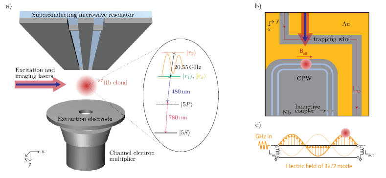
Figure 1: Schematics of the experimental system (not to scale). a An ultracold cloud of ⁸⁷Rb atoms is trapped at $130\,\mu$m distance from a CPW resonator. A pair of lasers with wavelengths $780\,$nm and $480\,$nm is used for two-photon excitation of the atoms from the ground state $\ket{5S}$ to a Rydberg state $\ket{r_{1}}$ (and $\ket{r_{x}}$) via an intermediate non-resonant state $\ket{5P}$. The MW coplanar waveguide cavity is inductively coupled via a feedline to an external MW source. In turn, the electric field of the cavity drives the atomic transition from state $\ket{r_{1}}$ to another Rydberg state $\ket{r_{2}}$, inducing damped Rabi oscillations. An extraction electrode below the cloud is used to apply a DC electric field for Stark-tuning the Rydberg transition frequency, for field-ionization of Rydberg atoms, and for extraction of the ions from the atom cloud. The ions are detected with a channel electron multiplier and adjacent detection electronics. b Bottom-view of the integrated superconducting atom chip containing a Z-shaped trapping wire and the CPW resonator: the trapping wire and the core of the MW resonator are made of superconducting niobium (gray); parts of the ground plane are coated with normal conducting gold (yellow); the bare sapphire chip surface is shown in blue. The magnetic trap with an offset field $B_{\mathrm{off}}$ at the center is generated by the current $I_{\mathrm{trap}}$ running through the trapping wire, persistent supercurrents around the cavity gaps, and external magnetic fields from macroscopic wires and coils bothner2013inductively . c Circuit scheme of the inductively-coupled superconducting transmission line cavity and the corresponding standing-wave electric field of the third harmonic frequency $\omega_{c}=2\pi\times 20.55$ GHz. The atom cloud is trapped near one of the electric field antinodes.

Our hybrid quantum system consists of a cloud of ultracold rubidium atoms trapped on an integrated superconducting (SC) atom chip containing a coplanar waveguide (CPW) resonator on the chip surface. Strong electric-dipole coupling between the atoms and the microwave (MW) cavity field requires, on the one hand, placing the atoms close to the chip surface, and, on the other hand, tuning the frequency of an appropriate Rydberg transition of the atoms into resonance with the fixed frequency of the cavity mode.

Experimental apparatus

The experimental system is illustrated in Fig. 1a. The experiment is performed in an ultra-high vacuum chamber at a pressure of $6\times 10^{-11}\,$mbar. The SC atom chip is attached to a He-flow cryostat with the surface temperature adjusted to 4.5 K. A chip-based magnetic trap for ultracold atoms is created via the field of the current in a Z-shaped trapping wire, the field associated with persistent SC currents in the resonator, and an external field generated by macroscopic wires and coils (see Fig. 1b). The resulting trapping potential, with an offset field of $3.4\,$G at the trap center, has a harmonic shape and can trap an atom cloud at a distance of $130\,\mu$m from the chip surface. A cloud of cold ⁸⁷Rb atoms is loaded to the magnetic trap and shifted into the field mode of the standing-wave MW resonator, similar to Refs. hattermann2017coupling ; bernon2013manipulation ; bothner2013inductively (see the Methods section M1 for more details). The atom cloud is positioned close to an electric-field antinode of the third harmonic mode of the MW resonator at frequency $\omega_{c}\simeq 2\pi\times 20.55$ GHz (see Fig. 1c). The resonator is inductively coupled via a feedline to an external coherent and tunable MW source. A laser system is used for imaging the atomic cloud and for Rydberg excitation of the atoms. A DC electric field applied via the electrode can state-selectively ionize the Rydberg state atoms and extract the resulting ions for detection via a channel electron multiplier (CEM).

Rydberg state excitation

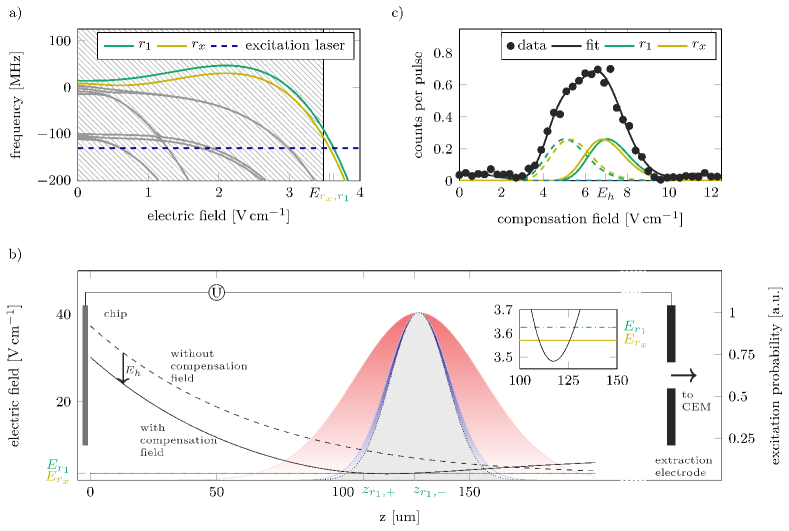
Figure 2: Laser excitation of Rydberg states of atoms in external fields. a Stark map of Rydberg states in the vicinity of the $48D$ state in a magnetic field of $3.4\,$G. The energies (frequency detuning relative to the $48D$ state in zero electric field) of the Stark states in the varying electric field are indicated by solid lines, while the dashed line indicates the frequency of the excitation laser detuned by $-2\pi\times 130\,$MHz. The target state $\ket{r_{1}}$ (green line) is resonantly excited by the laser in a field of $E_{r_{1}}=3.625\,$V/cm, and the nearby state $\ket{r_{x}}$ (yellow line) is resonant at $E_{r_{x}}=3.570\,$V/cm. Adsorbate field components parallel to the chip surface can not be compensated, preventing the excitation of Rydberg states in the hatched area. b Adsorbates on the chip surface produce an inhomogeneous electric field (black dashed line) that falls off exponentially with the distance from the surface. A voltage $U$ applied between the chip and the extraction electrode creates a homogeneous electric field of $E_{\mathrm{h}}=7.2\,$V/cm that partially compensates the $z$-component of the adsorbate field at the position of the atom cloud (red profile). This leads to a minimum of the total field (black solid line) at a distance of $z_{\mathrm{min}}=117\,\mu$m from the chip surface (see the inset for a magnified view of this area). Due to non-compensated field components in the $xy$ plane, the total field has a parabolic form around the minimum (see Methods section M2). State $\ket{r_{1}}$ is resonantly excited in thin atomic layers at positions $z_{r_{1}}=108\,\mu$m and $128\,\mu$m where the field is $E_{r_{1}}$, while state $\ket{r_{x}}$ is resonantly excited at positions $z_{r_{x}}=110\,\mu$m and $126\,\mu$m where the field is $E_{r_{x}}$. The excitation probability at each of these positions is proportional to the product (gray profile) of the cloud density (red profile) and the laser intensity (blue profile), and the corresponding atomic transition probabilities to states $\ket{r_{1}}$ and $\ket{r_{x}}$. Applying a high-voltage ramp between the chip and the extraction electrode results in field ionization of Rydberg atoms and acceleration of the resulting ions towards the ion detector (CEM). c Mean number of Rydberg excitations (ion counts, black dots) per laser pulse versus the applied compensation field. The experimental data is fitted by a sum of individual contributions from the $\ket{r_{1}}$ (green) and $\ket{r_{x}}$ (yellow) Rydberg states within two excitation layers (solid and dashed lines) each. From the fit we deduce the characteristic parameters of the adsorbate field.

The trapped atoms are excited from the ground state $\ket{5S}$ to a Rydberg state $\ket{r_{1}}$ (and to $\ket{r_{x}}$, see below) by a two-photon transition, via an intermediate non-resonant state $\ket{5P}$, using a pair of laser pulses with wavelengths $780\,$nm and $480\,$nm (see Methods section M1). The atoms are subject to a spatially varying DC (static) electric field, which is the sum of an inhomogeneous field produced by adsorbates on the chip surface tauschinsky2010spatially ; hattermann2012detrimental ; chan2014adsorbate ; sedlacek2016electric and a controlled homogeneous compensation field produced by the extraction electrode (see Fig. 1a). The electric field results in strong level shifts of the atomic Rydberg states. Figure 2a shows the calculated Stark map of Rydberg states in the vicinity of the zero-field $48D$ state, taking into account the offset magnetic field of the trap. The calculation employs a diagonalization of the atomic Hamiltonian in the presence of electric and magnetic fields zimmerman1979stark ; grimmel2015measurement , with the eigenvalues yielding the Rydberg energy spectrum for each field value.

The electric field of the adsorbates falls off exponentially from the chip surface. An appropriate voltage applied to the extraction electrode creates a homogeneous compensation field between the chip surface and the electrode, which cancels the $z$ component of the adsorbate field at a desired position $z_{\mathrm{min}}$ within the atomic cloud. Since the adsorbate field is inhomogeneous, the total field strength increases in both directions from $z_{\mathrm{min}}$ along $z$. Furthermore, the adsorbates produce a non-vanishing field component parallel to the chip surface, in the $xy$ plane, which cannot be compensated for in our setup. This field component thus determines the minimal achievable field strength, while the total electric field in $z$ direction acquires a parabolic form (see Fig. 2b and the Methods section M2). Hence, the resonance conditions for Rydberg excitations strongly vary across the atom cloud and each Rydberg state can be laser excited only in a thin ($\lesssim 0.3\,\mu$m) atomic layer. Since the energies of the Stark eigenstates depend only on the absolute value of the electric field, for each Rydberg state there are typically two resonant excitation layers, one on each side of the field minimum at $z_{\mathrm{min}}$ (see the inset of Fig. 2b). By varying the compensation field, these resonant layers can be shifted through the cloud with nearly constant layer separation.

To match the position of resonant layers with that of the atomic cloud and the excitation laser beams, we vary the compensation field and count the number of Rydberg atoms excited by the laser with fixed detuning $-2\pi\times 130\,$MHz with respect to the zero-field $48D_{5/2}$ state. To this end, we prepare cold atomic clouds in the mode volume of the CPW cavity, at a distance of $130\,\mu$m from the chip surface. Each of these clouds is exposed to a series of 300 excitation pulses of $1\,\mu$s duration, followed by Rydberg atom detection, at $3\,$kHz repetition rate, without significantly reducing the number of trapped atoms. After each pulse, the Rydberg excited atoms are ionized by a $1\,\mu$s electric field ramp and the resulting ions are subsequently detected by the CEM with a detection efficiency $>50$% stibor2007calibration ; guenther2009observing . Figure 2c shows the mean number of ion counts per excitation pulse as a function of the compensation field. We excite on average about one Rydberg atom per pulse, which allows us to disregard interactions between the Rydberg atoms. The resulting dependence of the ion count on the compensation field maps the atomic density distribution and the laser intensity profile in different excitation layers. The latter is deduced from fitting an appropriate model function to the experimental data (see Methods section M2). We then obtain that the exponential decay length of the adsorbate field from the chip surface is $\zeta\simeq 70\,\mu$m, while the field component parallel to the chip surface has a value of $3.482\,$V/cm. For a compensation field of $7.2\,$V/cm, only two Rydberg states $\ket{r_{1}}$ and $\ket{r_{x}}$ are excited with significant probabilities in the center of the atom cloud. The calculated two-photon transition amplitudes between the ground $\ket{5S}$ and the Rydberg states $\ket{r_{1}}$ and $\ket{r_{x}}$ are approximately equal, which corresponds to similar excitation numbers $N_{r_{1}}$ and $N_{r_{x}}$.

Tuning the Rydberg transition

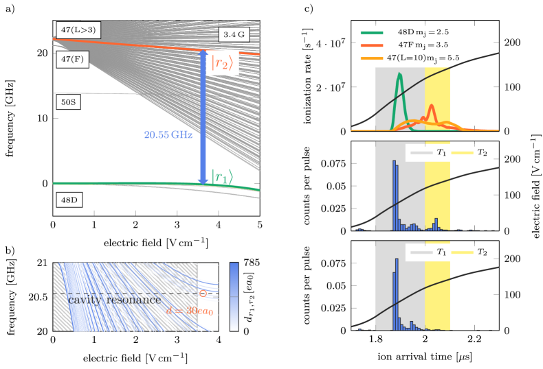
Figure 3: Rydberg transition and state detection. a Stark map of Rydberg states in the vicinity of $48D$ and $47(L\geq 3)$ states in a magnetic field of $3.4\,$G. State $\ket{r_{1}}$ (green line) is resonantly excited by a laser in an electric field of $E_{r_{1}}=3.625\,$V/cm (see Fig. 2a) and is coupled by a MW photon with frequency $\omega_{c}=2\pi\times 20.55\,$GHz to the Rydberg state $\ket{r_{2}}$ (red line) in the $47(L>3)$ manifold. b Frequencies (solid lines) and dipole moments (opacity) for transitions from state $\ket{r_{1}}$ to the states in the $n=47$ manifold, assuming in the calculations the total electric field along $x$, the magnetic field along $y$, and linear MW field polarization in the $z$ direction. The dashed horizontal line indicates the cavity resonance frequency $\omega_{c}$ and the transition to the resonant state $\ket{r_{2}}$ (red circle) has a dipole moment of $d=30ea_{0}$. c Upper panel: Examples of calculated ionization rates for three Rydberg states (green, red and orange lines) upon the electric field ramp (black line). Central panel: Histogram of the ion arrival times (blue bars) as measured for a laser Rydberg excitation followed by a MW $\pi$-pulse of $250\,$ns duration and a subsequent electric field ramp (black solid line). The data is averaged over 25 experimental cycles with 300 excitation-interaction-detection sequences in each cycle. Defining two time intervals $T_{1}$ and $T_{2}$ permits distinguishing the ion signal from states $\ket{r_{1}}$ and $\ket{r_{2}}$. Lower panel: Ion arrival time distribution without MW pulses.

With an atom in Rydberg state $\ket{r_{1}}$, depending on the total electric and magnetic fields at the atomic position, there are many possible MW transitions to the Rydberg states in the $n=47$ manifold. In Fig. 3a we show the calculated Stark map for the Rydberg states of atoms in the $3.4\,$G offset magnetic field of the trap and varying total electric field. Given the resonant frequency of the cavity field $\omega_{c}$ and the total electric field $E_{r_{1}}=3.625\,$V/cm at the position of the resonantly laser-excited layer of atoms in state $\ket{r_{1}}$, we deduce a suitable Rydberg transition to state $\ket{r_{2}}$ (see Fig. 3b). Our calculations also yield the dipole moments for different transitions (see Methods section M3) and we obtain the dipole moment $d\simeq 30ea_{0}$ for the $\ket{r_{1}}\to\ket{r_{2}}$ transition, while the differential Stark shift between levels $\ket{r_{1}}$ and $\ket{r_{2}}$ is rather small, $-163\,$MHz/(V/cm). Moreover, neighboring Rydberg states are sufficiently far off-resonant, which suppresses their excitation.

Rydberg ionization signal

Using the electric field ramp of the extraction electrode, we ionize the Rydberg state atoms and detect the resulting ions. In principle, each state ionizes under the influence of an electric-field ramp with a characteristic time dependence, which can be used to distinguish the Rydberg states gregoric2017quantum ; gurtler2004 . In general, states with higher principal quantum numbers $n$ tend to ionize earlier, while states with higher orbital angular momenta $L$ and magnetic quantum numbers $m_{j}$ are ionized later gallagher2005rydberg . In practice, the ionization signal from neighboring Rydberg states can have large temporal overlap, complicating their unambiguous discrimination. In Fig. 3c upper panel, we show three examples of calculated ionization signals from different Rydberg states subject to the same electric field ramp (see Methods section M4). If we divide the ion arrival times into two intervals $T_{1}$ and $T_{2}$, then during $T_{1}$ we will detect all the ions from state $48D$ and some of the ions from states $n=47$, while the ions detected during $T_{2}$ will only be from states $n=47$.

In the experiment, we populate via laser excitation states $\ket{r_{x}}$ and $\ket{r_{1}}$ with comparable probabilities, $N_{r_{x}}/N_{r_{1}}=a\approx 1$, and then couple $\ket{r_{1}}$ to state $\ket{r_{2}}$ via the resonant MW cavity field. The electric field ramp results in the Rydberg state ionization and detection of $N=N_{r_{x}}+N_{r_{1}}+N_{r_{2}}$ ions. All the ions $N_{r_{x}}$ and $N_{r_{1}}$ from states $\ket{r_{x}}$ and $\ket{r_{1}}$ are detected during the time interval $T_{1}=1.8-2.0\,\mu$s, while we estimate that the $N_{r_{2}}$ ions from state $\ket{r_{2}}$ are detected during the time interval $T_{2}=2.0-2.1\,\mu$s with probability $p=0.34$ and during $T_{1}$ with probability $(1-p)=0.66$. Hence, the number of ions $N_{T_{1}}$ and $N_{T_{2}}$ detected during $T_{1}$ and $T_{2}$ are $N_{T_{1}}=N_{r_{x}}+N_{r_{1}}+(1-p)N_{r_{2}}\simeq(1+a)(N_{r_{1}}+N_{r_{2}})-pN_{r_{2}}$ and $N_{T_{2}}=pN_{r_{2}}$, while $N_{T_{1}}+N_{T_{2}}=N$. We then obtain that the population of state $\ket{r_{2}}$ is $\rho_{22}\equiv\frac{N_{r_{2}}}{N_{r_{1}}+N_{r_{2}}}=\frac{(1+a)}{p}\frac{N_{T_{2}}}{N}=\frac{1+a}{p}p_{2}$, where $p_{2}\equiv N_{T_{2}}/N$.

In Fig. 3c middle panel, we show the measured ion signal after applying a MW $\pi$-pulse, which would ideally transfer all of the population of state $\ket{r_{1}}$ to state $\ket{r_{2}}$. The ion arrival times have a large peak in $T_{1}$ originating from all states $\ket{r_{x}}$, $\ket{r_{1}}$, $\ket{r_{2}}$, and a smaller peak in $T_{2}$ that we attribute only to state $\ket{r_{2}}$. With $N_{T_{1}}/N_{T_{2}}\approx 5.6$, the population of state $\ket{r_{2}}$ is $\rho_{22}\simeq 0.9$, consistent with a weakly damped half of a resonant Rabi cycle. Without the MW pulse, all the population remains in states $\ket{r_{x}}$ and $\ket{r_{1}}$ and no peak is observed in $T_{2}$, as shown in the lower panel of Fig. 3c.

Cavity driven Rydberg transition

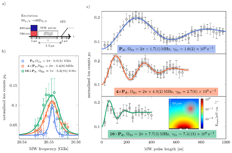
Figure 4: Coupling Rydberg transition to pumped MW cavity mode. a Schematics of the experimental sequence involving optical excitation of the atoms to the Rydberg state by a two-photon laser pulse of $1\,\mu$s duration, injection of a MW pulse of variable power and duration $\tau\leq 1.5\,\mu$s into the cavity, interaction of the Rydberg excited atoms with the MW cavity field, and selective field ionization (SFI) and detection of the Rydberg atoms by a $1\,\mu$s electric field ramp from $7.2\,$V/cm to about $210\,$V/cm. In each experimental cycle, the atom cloud is exposed to a series of $300$ excitation-interaction-detection sequences at a repetition rate of $3\,$kHz. MW leakage through the electronic switches and background counts lead to a small offset of the ion signal. b Normalized ion count $p_{2}=N_{T_{2}}/N$ (open circles), proportional to the population $\rho_{22}$ of Rydberg state $\ket{r_{2}}$, versus the frequency of the injected into the cavity MW pulses of duration $\tau=1.5\,\mu$s, for three different powers $P_{s},4P_{s},16P_{s}$ (blue, red, green) of the MW source. Each data point is obtained by averaging over 10 experimental cycles, with error bars denoting $\pm 2$ standard deviations. We fit the data by theoretical excitation spectra (solid lines of the same color) to deduce the Rabi frequencies $\bar{\Omega}$ of the MW field resonant with the $\ket{r_{1}}\to\ket{r_{2}}$ transition. c Dynamics of population of Rydberg state $\ket{r_{2}}$ (proportional to ion count $p_{2}$) for three different powers $P_{d},4P_{d},16P_{d}$ of the injected MW field at frequency $\omega_{\mathrm{MW}}=20.551\,$GHz. Each data point (open circle) is obtained by averaging over 25 experimental cycles, with error bars denoting $\pm 2$ standard deviations. Rabi frequencies $\Omega_{\mathrm{fit}}$ and decoherence rates $\gamma_{\mathrm{fit}}$ are obtained by fitting the model function (see the text and Methods section M5 for details), with the fitted curves (solid lines) shown with 95% confidence bounds (gray). The inset shows the MW cavity field strength in the $xz$ plane for a rms ground state voltage of $3\,\mu$V (see Methods section M3), with the cloud placed at a distance of $z\simeq 130\,\mu$m from the chip surface (bottom) and laterally displaced from the central cavity conductor by $x\simeq 50\,\mu$m. The gray bars indicate the position of the CPW.

Having described all the necessary ingredients of our system, we now turn to the demonstration of coherent coupling of the atomic Rydberg transition to an externally pumped MW field mode of the cavity. The experimental sequence is illustrated in Fig. 4a: after the two-photon laser excitation of the atoms to the Rydberg state $\ket{r_{1}}$, we inject into the cavity a MW pulse of variable power and duration. The Rydberg atom interacts with the cavity field on the transition $\ket{r_{1}}-\ket{r_{2}}$ for up to $1.5\,\mu$s. The cavity induced population transfer between the Rydberg states is then detected via selective field ionization and time-resolved ion counting.

The interaction of the atom with the MW cavity field can be well approximated by a two-level model. The field mode of the cavity with frequency $\omega_{c}=2\pi\times 20.55\,$GHz is resonant with the atomic transition $\ket{r_{1}}-\ket{r_{2}}$, while the next nearest Rydberg transition is detuned by at least $15\,$MHz (see Fig. 3b), which exceeds the cavity linewidth $\kappa=2\pi\times 9\,$MHz and the maximal achieved Rabi frequency $\Omega_{\mathrm{max}}\simeq 2\pi\times 8\,$MHz. There are no near resonant transitions from state $\ket{r_{x}}$. Decay to other states is negligible during the entire excitation, interaction and measurement time of $\sim 3\,\mu$s, which is much shorter than the Rydberg state lifetime $1/\Gamma\approx 60\,\mu$s mack2015all ; beterov2009quasiclassical .

In Fig. 4b we show the Rydberg transition spectrum of the atoms interacting with the intracavity MW field pumped by the external source of variable frequency at three different powers. The exposure time of $1.5\,\mu$s is sufficiently long for the atomic populations to attain the steady state. We fit the observed spectrum with a model function corresponding to the steady-state population $\rho_{22}$ of the Rydberg state $\ket{r_{2}}$, while the Rabi frequency of the MW field also depends on the frequency of the injected into the cavity field (see Methods section M5). We assume that the main contribution to the atomic spectral linewidth comes from the inhomogeneous broadening $\Delta\omega_{12}\simeq 2\pi\times 1.1\,$MHz of the transition $\ket{r_{1}}-\ket{r_{2}}$ due to the differential Stark shift of $-163\,$MHz/(V/cm) between levels $\ket{r_{1}}$ and $\ket{r_{2}}$ in the inhomogeneous electric field varying by $0.0067\,$V/cm within the resonantly excited atomic layer of widths $\lesssim 0.3\,\mu$m (see Methods section M3). In comparison, the natural linewidth (decay rate) $\Gamma\simeq 2\pi\times 2.7\,$kHz of the Rydberg state is negligible. For stronger pumping fields, the spectrum is dominated by power broadening.

For each pumping power, we extract the peak Rabi frequency $\bar{\Omega}$ at the pump MW frequency $\omega_{\mathrm{MW}}\simeq\bar{\omega}_{12}$ resonant with the mean transition frequency of the atoms in the resonant layer. We then obtain that the peak Rabi frequency $\bar{\Omega}$ scales approximately as square root of the pumping power $P$, as expected for a resonant one-photon transition.

By changing the detuning of the excitation lasers, we can excite the Rydberg states of atoms in a different resonant layer. This in turn will shift the atomic Rydberg transition out of the cavity resonance, causing the signal in Fig. 4b to disappear. Using a MW antenna from outside the chamber, we can recover the ionization signal for an appropriate MW frequency, which verifies that the Rydberg MW transition is indeed driven by the cavity field. The cavity and the atomic resonance are, however, not perfectly aligned, which leads to a small asymmetry of the resonance profiles that becomes more pronounced for increasing MW power, as seen in Fig. 4b.

We next fix the frequency of the injected MW field to $\omega_{\mathrm{MW}}=2\pi\times 20.551\,$GHz, and investigate the dynamics of the Rydberg transition by varying the duration of the MW pulse for three different input powers. In Fig. 4c we show the normalized ion count $p_{2}$ from the upper Rydberg state $\ket{r_{2}}$ as a function of the MW pulse duration. We observe damped Rabi oscillations between states $\ket{r_{1}}$ and $\ket{r_{2}}$ with the Rabi frequencies that scale approximately as $\Omega\propto\sqrt{P}$, similarly to the steady-state case above. We approximate the population difference between the Rydberg states as $\bar{D}=\rho_{11}-\rho_{22}=\exp(-t^{2}/\tau_{\mathrm{damp}}^{2})\cos(\bar{\Omega}t)$, which follows from a simple model (see Methods section M5) that assumes two-level atoms coherently driven by spatially varying Rabi frequencies corresponding to an inhomogeneous MW cavity field distribution across the laterally displaced atomic ensemble, as shown in the inset of Fig. 4c. The corresponding damping rate $\gamma=1/\tau_{\mathrm{damp}}$ then scales approximately linearly with the Rabi frequency, $\gamma\simeq\frac{b}{\sqrt{2}}\bar{\Omega}$ with the proportionality constant $b\approx 0.2$ that quantifies the relative change of cavity MW field across the atomic cloud along the $x$ direction.

Discussion

We have demonstrated coherent coupling of ultracold Rb atoms, trapped on an integrated atom chip and laser excited to the Rydberg states, to a superconducting MW resonator. We used DC electric fields to fine-tune the atomic Rydberg transition and observed resonant Rabi oscillations between a pair of Rydberg states driven by the MW field of the cavity pumped by an external coherent source. The observed damping of the Rabi oscillations in our system is dominated by the spread of Rabi frequencies for the Rydberg atoms in different positions of the resonantly excited by the laser layer. In comparison, the real single atom decoherence is much smaller, and individual Rydberg atoms are expected to exhibit much longer coherence times.

We note, that the damping rate of the Rabi oscillations originating from the variations of the cavity field at different positions within the atom cloud is significantly reduced by the resonant laser excitation of Rydberg states of atoms in a thin layer at a well defined distance from the atom chip. Better positioning of the atomic cloud, reducing the lateral size of the excitation layer, and using narrow-line excitation lasers can further reduce or completely eliminate the cavity field variations for the Rydberg excited atoms, leading to much longer coherence times of the MW Rydberg transition of the atoms.

The atoms in our system are trapped relatively far from the CPW cavity, $130\,\mu$m from the chip surface, and the resulting vacuum Rabi frequency $\Omega_{\mathrm{vac}}=dE_{c}^{(0)}/\hbar=2\pi\times 0.6\,$kHz is much smaller than the cavity linewidth $\kappa\simeq 2\pi\times 9\,$MHz. Several improvements can be made: The atoms can be brought much closer to the chip surface and, e.g., at a distance of $\sim 10\,\mu$m the cavity field strength $E_{c}^{(0)}$ will increase by more than an order of magnitude. At smaller distances, the stronger adsorbate fields should be treated more carefully and a pair of Rydberg-Stark eigenstates with much larger dipole moments $d\simeq 10^{3}ea_{0}$ and small differential Stark shift should be found and used. Furthermore, there has been great progress in increasing the quality factors of superconducting coplanar waveguide resonators, already exceeding $10^{6}$ at $\sim 50\,$mK temperatures megrant2012planar , which also enables coherent operations of SC qubits. This will then bring the strong-coupling regime of single Rydberg atoms and SC qubits to single MW cavity photons within the experimental reach.

Methods

M1 EXPERIMENTAL SYSTEM

Atomic cloud. Starting with ⁸⁷Rb atoms in a conventional magneto-optical trap, about $5\times 10^{7}$ atoms in the ground state $\ket{5S_{1/2},F=2,m_{F}=2}$ are loaded into a magnetic quadrupole trap. The atoms are then moved to a Ioffe trap for evaporative cooling. Using optical tweezers, the ultracold atomic cloud is transferred to a superconducting atom chip, which is mounted on the cold-finger of a He-flow cryostat. At the chip, the spin-polarized atomic cloud is loaded into a magnetic microtrap generated by a current in the Z-shaped trapping wire and other external homogeneous fields. Additional bias fields are used to finally position the cloud close to a coplanar waveguide resonator. Using standard absorption imaging, we verify that the cloud is trapped at $130\,\mu$m distance to the chip surface. The trapping potential has a parabolic shape with trap frequencies $\omega_{x,y,z}=2\pi\times 61$ Hz. The offset field at the trap center is about $3.4\,$G. The atom cloud has spherical shape with a cloud diameter (full width at half maximum) of $60\,\mu$m. The atom number in the cloud is $7\times 10^{4}$, the peak density is $2.7\times 10^{11}\,\mathrm{cm}^{-3}$ and the temperature is $1\,\mu$K. More details on the loading and trapping procedure are given in Ref. hattermann2017coupling .

Rydberg lasers. The atoms are excited from the ground state $\ket{5S_{1/2}}$ to the Rydberg states by a pair of laser pulses with wavelengths $780\,$nm and $480\,$nm and duration of $1\,\mu$s, while the intermediate state $\ket{5P_{3/2}}$ is detuned by $160\,$MHz. Both laser beams are centered at the atomic cloud. With beam waists ($1/e^{2}$-radii) of $5.45\,$mm and $0.025\,$mm and laser powers of $0.5\,$mW and $25\,$mW, the peak intensities of the red and blue lasers are $0.001\,$W/cm² and $2500\,$W/cm², respectively. The red laser is phase locked to a commercial frequency comb with an absolute frequency accuracy of $2\,$kHz and linewidth below $10\,$kHz. The blue laser is stabilized with a wavelength meter (HighFinesse WSU) to an absolute frequency accuracy better than $2\,$MHz and a linewidth better than $200\,$kHz. In zero field conditions, the single-photon Rabi frequencies for individual transitions $5S_{1/2}-5P_{3/2}$ and $5P_{3/2}-48D_{5/2}$, averaged over all magnetic sub-states and possible transitions, are $2\pi\times 3.6\,$MHz and $2\pi\times 36\,$MHz, respectively. The resulting effective two-photon Rabi-frequency for the Rydberg excitation $5S_{1/2}-48D_{5/2}$ is $2\pi\times 400\,$kHz. Taking into account the external fields and applying the selection rules for appropriate laser polarization, the two-photon Rabi-frequency for the transition $\ket{5S_{1/2},F=2,m_{F}=2}\to\ket{r_{1}}$ and $\ket{r_{x}}$ is reduced to about $\Omega_{gr}=2\pi\times 30\,$kHz; the ratio $a$ between these Rabi frequencies depends on the unknown direction of the lateral surface field (see Sec. M2 below) and is assumed $a\approx 1$. With this Rabi frequency and a pulse duration of $1\,\mu$s applied to the ensemble of $7\times 10^{4}$ ground state atoms, we excite on average about one atom to the Rydberg state $\ket{r_{1}}$.

Microwave cavity. The on-chip superconducting coplanar waveguide cavity is a $\lambda/2$ transmission line resonator with the fundamental mode frequency $\omega_{0}=2\pi\times 6.85\,$GHz. To drive the transition between the Rydberg states $\ket{r_{1}}$ and $\ket{r_{2}}$, we use the third harmonic mode of the resonator having the frequency $\omega_{c}=2\pi\times 20.55\,$GHz, the linewidth $\kappa=2\pi\times 9\,$MHz and the corresponding quality factor $Q\approx 2300$. Within the temperature range where the resonator is superconducting, the resonance frequency can be tuned by about $30\,$MHz. For driving purposes, the resonator is inductively coupled to a MW feedline and connected to a commercial MW signal generator (Rohde & Schwarz SMF100A) with a linewidth $<1\,$Hz. The MW electric field in the resonator is then

$$E_{c}\propto\frac{\sqrt{P}}{\kappa/2-i(\omega_{\mathrm{MW}}-\omega_{c})},$$ (1)

where $P$ is the power of the injected into the resonator MW field at frequency $\omega_{\mathrm{MW}}$.

M2 RYDBERG EXCITATION

Surface fields. The adsorbates on the chip surface produce an inhomogeneous electric field. We approximate the $z$ component of this adsorbate field perpendicular to the chip surface as $E_{\mathrm{ad},z}(z)=E_{0}e^{-z/\zeta}$, where $\zeta$ is a decay length. This component is partially compensated by a homogeneous field $E_{\mathrm{h}}$ between the extraction electrode and the grounded atom chip surface. The compensation field can be freely adjusted by the voltage $U$ applied to the extraction electrode, $E_{\mathrm{h}}/U=3\,$(V/cm)/V. The inhomogeneous adsorbate distribution leads to an additional field component parallel to the chip surface, $E_{\mathrm{ad},xy}$, which can not be compensated for in our system. The total electric field

$$E(z)=\sqrt{(E_{0}e^{-z/\zeta}-E_{\mathrm{h}})^{2}+E_{\mathrm{ad},xy}^{2}}$$ (2)

can then be tuned via $E_{\mathrm{h}}$ and has a parabolic form around the field minimum $E(z_{\mathrm{min}})=E_{\mathrm{ad},xy}$ at $z_{\mathrm{min}}=\zeta\ln\frac{E_{0}}{E_{\mathrm{h}}}$.

Excitation layers. The Stark shifts of the atomic Rydberg levels in a DC electric field depend only on the absolute field strength. Within the atomic cloud, there can be two layers where the electric field has a specific value $E_{r}>E(z_{\mathrm{min}})=E_{\mathrm{ad},xy}$. These layers are positioned on both sides of the field minimum at

$$z_{r,\pm}=z_{\mathrm{min}}-\zeta\ln{\left(1\pm\sqrt{\frac{E_{r}^{2}-E_{\mathrm{ad},xy}^{2}}{E_{\mathrm{h}}^{2}}}\right)}.$$ (3)

A Rydberg state $\ket{r}$ that is resonant at a specific field strength $E_{r}$ is thus excited in two excitation layers at position $z_{r,\pm}$. For a field $E_{r}=E_{\mathrm{ad},xy}$ both layers merge at $z_{r,\pm}=z_{\mathrm{min}}$, while no excitation can take place for states that are resonant in fields $E_{r}<E_{\mathrm{ad},xy}$.

The local field gradient in a resonant excitation layer is

$$\alpha_{r,\pm}=\left.\frac{dE}{dz}\right|_{z_{r,\pm}}=\frac{1}{\zeta}\frac{E_{\mathrm{h}}^{2}}{E_{r}}(\beta\mp\sqrt{\beta_{r}})$$ (4)

with $\beta_{r}=\sqrt{E_{r}^{2}-E_{\mathrm{ad},xy}^{2}}/E_{\mathrm{h}}$. Assuming the two-photon Rabi frequency $\Omega_{gr}$ is small compared to the linewidth of the excitation laser $\Delta\omega_{\mathrm{las}}$, the width of the excitation layer can be estimated as

$$\Delta z_{r,\pm}=\frac{\Delta\omega_{\mathrm{las}}}{d_{r}\alpha_{r,\pm}},$$ (5)

where $d_{r}$ is the Stark gradient, or static dipole moment, of state $\ket{r}$.

Excitation probability With the excitation layers oriented parallel to the chip surface, the Rydberg excitation probability of the atoms within a single layer at $z$ is proportional to the atomic line density and the laser intensity profile,

$$n(z) \propto \exp{\left(-\frac{(z-z_{\mathrm{cloud}})^{2}}{2\sigma^{2}}\right)},$$ (6)

$$I(z) \propto \exp{\left(-\frac{2(z-z_{\mathrm{beam}})^{2}}{w^{2}}\right)},$$ (7)

where $z_{\mathrm{cloud}}$ is the position of the atomic cloud, $\sigma$ is the cloud radius, $z_{\mathrm{beam}}$ is the laser beam center and $w$ is the beam waist. For a two-photon transition, $\Omega_{gr}\propto\sqrt{I_{780}I_{480}}$, the effective beam waist is $w=w_{780}w_{480}/\sqrt{w_{780}^{2}+w_{480}^{2}}$ with the individual beam waists $w_{780,480}$ assumed to overlap at the same position. The total Rydberg excitation probability is given by the sum over all possible transitions in the corresponding excitation layers:

$$P_{\mathrm{Ry}}=\sum_{r}\sum_{s=\pm}A_{r,s}\,n(z_{r,s})\,I(z_{r,s})$$ (8)

where the strength coefficients $A_{r,\pm}$ depend on the dipole matrix element of the corresponding transition.

Fit to the data. We use Eq. (8) to fit the experimental data in Fig. 2c taking into account all states and their corresponding excitation layers. For each state $\ket{r}$, we determine the resonance field value $E_{r}$ from the Rydberg Stark map calculations in Fig. 2a with the excitation laser detuning set to $-130\,$MHz with respect to the zero-field $48D_{5/2}$ state. Atomic cloud and beam parameters are $z_{\mathrm{cloud}}=z_{\mathrm{beam}}=130\,\mu$m, $\sigma=25\,\mu$m and $w\approx w_{480}=25\,\mu$m, leaving only the strength coefficients $A_{r}$ and the adsorbate field parameters $E_{0}$, $\zeta$ and $E_{\mathrm{ad},xy}$ as free fitting parameters. We then obtain $E_{0}=37.2\,$V/cm, $\zeta=70\,\mu$m and $E_{\mathrm{ad},xy}=3.482\,$V/cm. Rydberg excitations mostly occur in the resonant excitation layers of the two states $\ket{r_{1}}$ and $\ket{r_{x}}$, as other states can be resonantly excited in different electric fields, at positions outside of the atomic cloud.

For a compensation field of $E_{\mathrm{h}}=7.2\,$V/cm, the two excitation layers for state $\ket{r_{1}}$ (resonant with the excitation laser at total field $E_{r_{1}}=3.625\,$V/cm) are located at $z_{r_{1},+}=108\,\mu$m and $z_{r_{1},-}=128\,\mu$m. With the two-photon excitation linewidth $\Delta\omega_{\mathrm{las}}=2\pi\times 2\,$MHz, the Stark gradient $d_{r_{1}}=-300\,$MHz/(V/cm) and the field gradients $\alpha_{r_{1},\pm}$, the corresponding layer widths are $\Delta z_{r_{1},+}=0.21\,\mu$m and $\Delta z_{r_{1},-}=0.28\,\mu$m. Since the atomic cloud is centered at $z=130\,\mu$m, dominant excitation takes place in the $z_{r_{1},-}$ layer. Energetically close states are excited in layers at different distances from the chip. They contribute to the ion signal, but do not participate in the MW transition between the Rydberg states and therefore only affect the contrast in the Rabi oscillation measurements.

M3 MICROWAVE RYDBERG TRANSITION

Matrix elements. The energy spectrum of Rydberg states in external fields can be calculated by diagonalization of the atomic Hamiltonian, including the interactions with the magnetic and electric fields, in the basis of zero-field states $\ket{n,l,j,m_{j}}$ zimmerman1979stark . We compute the energy eigenvalues and the corresponding eigenvectors

$$\ket{r}=\sum_{n,l,j,m_{j}}\beta^{n,l,j,m_{j}}\ket{n,l,j,m_{j}},$$ (9)

where $\beta^{n,l,j,m_{j}}$ are the normalized amplitudes of the basis states. The dipole moment for the transition between a pair of Rydberg states $\ket{r_{i}}$ and $\ket{r_{f}}$ is then grimmel2015measurement

$$\vec{d}=e\braket{r_{f}}{\vec{r}}{r_{i}}=e\sum_{q}\sum_{q^{\prime}}\beta_{f}^{q^{\prime}\ast}\beta_{i}^{q}\braket{q^{\prime}}{\vec{r}}{q}$$ (10)

where $e$ is the electron charge and $\vec{r}$ is its position vector, while $q^{(\prime)}$ denote the full set of quantum numbers $n,l,j,m_{j}$. Note that for an atom subject to only a magnetic or electric field, only a subset of basis states, determined by the selection rules, can be used for the diagonalization. But in combined electric and magnetic fields, all the zero-field basis states with different quantum numbers $l$ and $m_{j}$ should be included, and already for small fields a set of more than 15000 basis states are required for the results of diagonalization to converge.

The precise polarization of the MW field with respect to the directions of the electric and magnetic fields at the excitation position is difficult to measure or simulate. Our calculations of the Rydberg state energies and transition dipoles as per Eqs. (9) and (10), assuming the magnetic field of $3.4\,$G along the $y$-direction, the electric field of $3.625\,$V/cm in the $x$-direction and a MW field polarization in $z$-direction, well reproduce the observed transition frequencies, and we obtain the dipole moment $d\simeq 30ea_{0}$ for the Rydberg transition $\ket{r_{1}}\to\ket{r_{2}}$. Changing the field strengths and directions can change the resulting transition dipole moment.

Vacuum Rabi frequency. The electric field energy in the cavity per MW photon is $CU_{c}^{2}=\hbar\omega_{c}$. With the cavity length $l=9.3\,$mm and the capacitance per unit length $C/l=164\,$pF/m, the (rms) ground state voltage on the central conductor is $U_{c}=3\,\mu$V. The resulting electric field per cavity photon at the position of the atoms $z=130\,\mu$m below the chip surface and $0.85\,$mm away from the antinode is $E_{c}^{(0)}(z)=0.015\,$mV/cm and varies by about 30% over the extent of the cloud. With the MW polarization along the transition dipole moment, the vacuum Rabi frequency is then $\Omega_{\mathrm{vac}}=dE_{c}^{(0)}/\hbar=2\pi\times 0.6\,$kHz.

Rydberg transition linewidth. The Stark gradients (static dipole moments) of the Rydberg states $\ket{r_{1}}$ and $\ket{r_{2}}$ are $d_{r_{1}}=-300\,$MHz/(V/cm) and $d_{r_{2}}=-463\,$MHz/(V/cm), leading to a differential Stark shift coefficient $\Delta d_{r}=d_{r_{2}}-d_{r_{1}}=-163\,$MHz/(V/cm). As described above, a laser with linewidth $\Delta\omega_{\mathrm{las}}=2\pi\times 2\,$MHz excites the atoms to the Rydberg state $\ket{r_{1}}$ in a layer of width $\Delta z_{r_{1},-}=0.28\,\mu$m, where the electric field varies by $\Delta z_{r_{1},-}\alpha_{r_{1},-}=\Delta\omega_{\mathrm{las}}/d_{r_{1}}$, as per Eqs. (4) and (5). Hence, the Rydberg transition $\ket{r_{1}}\to\ket{r_{2}}$ for the atoms in this layer is inhomogeneously broadened by the spatially varying electric field by

$$\Delta\omega_{12}\simeq\Delta z_{r_{1},-}\alpha_{r_{1},-}\Delta d_{r}=\Delta\omega_{\mathrm{las}}\frac{\Delta d_{r}}{d_{r_{1}}}\simeq 2\pi\times 1.1\,\mathrm{MHz}.$$ (11)

M4 IONIZATION SIGNAL

The selective field ionization (SFI) signal for a specific Rydberg state and electric field ramp is calculated by following the time evolution of the atomic population through the Stark map, using the diagonalization of the Hamiltonian matrix with $2\,$ns step size. At each time step and for each state, an ionization rate is calculated using a complex absorbing potential, $\mathrm{CAP}=-i\eta W(\hat{r},F_{E})$, added to the Hamiltonian, with the scaling parameter $\eta=1.52\cdot 10^{-10}E_{H}/a_{0}$ (with Hartree energy $E_{H}$ and Bohr radius $a_{0}$), a $r^{6}$ radius dependence and a shift with the external electric field $F_{E}$ grimmel2017ionization . The time dependence of the electric field corresponds to the voltage ramp at the extraction electrode, while the SFI signal has a time delay of $1.53\,\mu$s equal to the time of flight of the ions in the experiment.

To limit the number of basis states and speed up calculations, the magnetic field is neglected during the ionization process, avoiding thereby mixing the different $m_{j}$ states in the electric field. This is justified as the interaction with the electric field is much stronger than the interactions with the magnetic field during the SFI field ramp. The SFI signal for different $m_{j}$ states can then be calculated separately.

The initial Rydberg states correspond to the Stark eigenstates in the combined magnetic and electric fields. The state $\ket{r_{1}}$ has sizable contributions only from the $m_{j}=-5/2\,...\,5/2$ substates of the $48D_{5/2}$ state, while the state $\ket{r_{2}}$ is given by a linear combination of zero-field states with different $l$ and $m_{j}$ values of the $n=47$ manifold. The resulting signal is then given by the sum over individually calculated (interpolated for all $l$ and $m_{j}$ values) ion signals weighted by the initial population distribution.

M5 CAVITY DRIVEN RYDBERG TRANSITION

Steady-state Rydberg spectrum. We model the interaction of an atom on the Rydberg transition $\ket{r_{1}}\to\ket{r_{2}}$ with the MW field by a driven two-level system. With the Rabi frequency $\Omega$, the decay rate $\Gamma$ and the resonant Rydberg transition frequency $\omega_{12}$, the steady state population of $\ket{r_{2}}$ is PLDP2007

$$\rho_{22}=\frac{|\Omega|^{2}/4}{\left(\omega_{\mathrm{MW}}-\omega_{12}\right)^{2}+\Gamma^{2}/4+|\Omega|^{2}/2}.$$ (12)

To account for the Rydberg transition linewidth, we assume that the transition frequencies are distributed according to a Gaussian function

$$S(\omega_{12})\propto\exp{\left(-\ln 2\left(\frac{\omega_{12}-\bar{\omega}_{12}}{\Delta\omega_{12}/2}\right)^{2}\right)},$$ (13)

where $\bar{\omega}_{12}$ is the mean transition frequency of the atoms in the resonant layer, and $\Delta\omega_{12}$ is the full width at half maximum. The appropriately weighted Rydberg state population is then

$$\tilde{\rho}_{22}=\int S(\omega_{12})\rho_{22}(\omega_{12})\,d\omega_{12}.$$ (14)

The atoms interact with the intracavity MW field with Rabi frequency $\Omega=dE_{c}/\hbar$, where $E_{c}$ is given by Eq. (1). We denote by $\bar{\Omega}\equiv\Omega(\omega_{\mathrm{MW}}=\bar{\omega}_{12})$ the Rabi frequency of the injected MW field resonant with mean transition frequency $\bar{\omega}_{12}$ of the atoms in the resonant layer. We can then write

$$|\Omega(\omega_{\mathrm{MW}})|^{2}=|\bar{\Omega}|^{2}\frac{(\bar{\omega}_{12}-\omega_{c})^{2}+\kappa^{2}/4}{(\omega_{\mathrm{MW}}-\omega_{c})^{2}+\kappa^{2}/4}.$$ (15)

The combination of Eqs. (12)-(15) then yields the model function $p_{2}=\frac{p}{1+a}\tilde{\rho}_{22}+p_{0}$ for the normalized ion counts $p_{2}$ which we use to fit the data in Fig. 4b with the offset $p_{0}$, the amplitude $p/(1+a)$ and additional fitting parameters $\bar{\Omega}$, $\bar{\omega}_{12}$ and $\omega_{c}$. From the fit we deduce $\bar{\omega}_{12}=2\pi\times 20.5513\,$GHz, $\omega_{c}=2\pi\times 20.5495\,$GHz, and $p/(1+a)\approx 0.2$.

Resonant Rabi oscillations. For a resonantly driven two-level atom, neglecting the population decay and coherence relaxation, the population difference between the states $\ket{r_{1}}$ and $\ket{r_{2}}$ is

$$D(\Omega,t)=\rho_{11}-\rho_{22}=\cos(\Omega t).$$ (16)

With the atomic cloud being laterally displaced by $x_{0}\simeq 50\,\mu$m from the cavity center (see the inset in Fig. 4c), the MW field strength varies in the resonant atomic layer. We assume that the corresponding Rabi frequency varies approximately linearly in space,

$$\Omega(x)=\bar{\Omega}\left(1+\frac{x-x_{0}}{\chi}\right).$$ (17)

The atomic density distribution in the layer is Gaussian, $n(x)\propto\frac{1}{\sqrt{2\pi}\sigma}\exp{\left(-\frac{(x-x_{0})^{2}}{2\sigma^{2}}\right)}$. For the spatially averaged population difference we then obtain

$$\bar{D}(t)=\int_{-\infty}^{-\infty}n(x)D\big{(}\Omega(x),t\big{)}\,dx=e^{-\gamma^{2}t^{2}}\cos(\bar{\Omega}t)$$ (18)

where $\gamma^{2}=\frac{\sigma^{2}}{2\chi^{2}}\bar{\Omega}^{2}$. Hence, the spatial variation of the MW field leads to damping of the resonant Rabi oscillations, even if we neglect the decay and coherence relations of the atoms.

From the MW field simulations, we estimate the relative change of the Rabi frequency across the cloud of width $\sigma=25\,\mu$m to be $b=\sigma/\chi\lesssim 0.3$, consistent with the observations in Fig. 4c, where we have $\gamma_{\mathrm{fit}}=1.6\pm 0.2\,\mu\mathrm{s}^{-1}$, $2.7\pm 0.6\,\mu\mathrm{s}^{-1}$, and $7.5\pm 1.3\,\mu\mathrm{s}^{-1}$ for $\Omega_{\mathrm{fit}}=2\pi\times 1.7\pm 0.1\,$MHz, $\Omega_{\mathrm{fit}}=2\pi\times 4.3\pm 0.2\,$MHz and $\Omega_{\mathrm{fit}}=2\pi\times 7.7\pm 0.3\,$MHz, respectively.

References

- (1) Xiang, Z.-L., Ashhab, S., You, J. & Nori, F. Hybrid quantum circuits: Superconducting circuits interacting with other quantum systems. Reviews of Modern Physics 85, 623 (2013).
- (2) Kurizki, G. et al. Quantum technologies with hybrid systems. Proceedings of the National Academy of Sciences 112, 3866–3873 (2015).
- (3) Schoelkopf, R. J. & Girvin, S. M. Wiring up quantum systems. Nature 451, 664–9 (2008).
- (4) Devoret, M. H. & Schoelkopf, R. J. Superconducting circuits for quantum information: an outlook. Science 339, 1169–74 (2013).
- (5) Lvovsky, A. I., Sanders, B. C. & Tittel, W. Optical quantum memory. Nat. Photonics 3, 706–714 (2009).
- (6) Fleischhauer, M., Imamoglu, A. & Marangos, J. P. Electromagnetically induced transparency: Optics in coherent media. Rev. Mod. Phys. 77, 633–673 (2005).
- (7) Hammerer, K., Sørensen, A. S. & Polzik, E. S. Quantum interface between light and atomic ensembles. Rev. Mod. Phys. 82, 1041–1093 (2010).
- (8) Blais, A., Huang, R.-S., Wallraff, A., Girvin, S. M. & Schoelkopf, R. J. Cavity quantum electrodynamics for superconducting electrical circuits: An architecture for quantum computation. Phys. Rev. A 69, 062320 (2004).
- (9) Zhu, X. et al. Coherent coupling of a superconducting flux qubit to an electron spin ensemble in diamond. Nature 478, 221–4 (2011).
- (10) Kubo, Y. et al. Hybrid quantum circuit with a superconducting qubit coupled to a spin ensemble. Phys. Rev. Lett. 107, 220501 (2011).
- (11) Saito, S. et al. Towards realizing a quantum memory for a superconducting qubit: storage and retrieval of quantum states. Phys. Rev. Lett. 111, 107008 (2013).
- (12) Sárkány, L., Fortágh, J. & Petrosyan, D. Faithful state transfer between two-level systems via an actively cooled finite-temperature cavity. Phys. Rev. A 97, 032341 (2018).
- (13) Treutlein, P., Hommelhoff, P., Steinmetz, T., Hänsch, T. W. & Reichel, J. Coherence in microchip traps. Phys. Rev. Lett. 92, 203005 (2004).
- (14) Fortágh, J. & Zimmermann, C. Magnetic microtraps for ultracold atoms. Rev. Mod. Phys. 79, 235–289 (2007).
- (15) Roux, C. et al. Bose-Einstein condensation on a superconducting atom chip. Europhys. Lett. 81, 56004 (2008).
- (16) Hermann-Avigliano, C. et al. Long coherence times for Rydberg qubits on a superconducting atom chip. Phys. Rev. A 90, 040502 (2014).
- (17) Rabl, P. et al. Hybrid quantum processors: molecular ensembles as quantum memory for solid state circuits. Phys. Rev. Lett. 97, 033003 (2006).
- (18) Verdú, J. et al. Strong magnetic coupling of an ultracold gas to a superconducting waveguide cavity. Phys. Rev. Lett. 103, 043603 (2009).
- (19) de Hond, J. et al. From coherent collective excitation to Rydberg blockade on an atom chip. Phys. Rev. A 98, 062714 (2018).
- (20) Petrosyan, D., Mølmer, K., Fortágh, J. & Saffman, M. Microwave to optical conversion with atoms on a superconducting chip. New J. Phys. 073033 (2019).
- (21) Petrosyan, D. & Fleischhauer, M. Quantum information processing with single photons and atomic ensembles in microwave coplanar waveguide resonators. Phys. Rev. Lett. 100, 170501 (2008).
- (22) Petrosyan, D. et al. Reversible state transfer between superconducting qubits and atomic ensembles. Physical Review A 79, 040304 (2009).
- (23) Hogan, S. D. et al. Driving Rydberg-Rydberg transitions from a coplanar microwave waveguide. Phys. Rev. Lett. 108, 063004 (2012).
- (24) Haroche, S. Nobel Lecture: Controlling photons in a box and exploring the quantum to classical boundary. Rev. Mod. Phys. 85, 1083 (2013).
- (25) Hermann-Avigliano, C. et al. Long coherence times for Rydberg qubits on a superconducting atom chip. Phys. Rev. A 90, 040502 (2014).
- (26) Morgan, A. & Hogan, S. Coupling Rydberg atoms to microwave fields in a superconducting coplanar waveguide resonator. Phys. Rev. Lett. 124, 193604 (2020).
- (27) Hattermann, H. et al. Coupling ultracold atoms to a superconducting coplanar waveguide resonator. Nat. Commun. 8, 2254 (2017).
- (28) Pritchard, J. D., Isaacs, J. A., Beck, M. A., McDermott, R. & Saffman, M. Hybrid atom-photon quantum gate in a superconducting microwave resonator. Phys. Rev. A 89, 010301 (2014).
- (29) Sárkány, L., Fortágh, J. & Petrosyan, D. Long-range quantum gate via Rydberg states of atoms in a thermal microwave cavity. Physical Review A 92, 030303 (2015).
- (30) Gard, B. T., Jacobs, K., McDermott, R. & Saffman, M. Microwave-to-optical frequency conversion using a cesium atom coupled to a superconducting resonator. Phys. Rev. A 96, 013833 (2017).
- (31) Covey, J. P., Sipahigil, A. & Saffman, M. Microwave-to-optical conversion via four-wave mixing in a cold ytterbium ensemble. Phys. Rev. A 100, 012307 (2019).
- (32) Tian, L., Rabl, P., Blatt, R. & Zoller, P. Interfacing quantum-optical and solid-state qubits. Phys. Rev. Lett. 92, 247902 (2004).
- (33) Bothner, D. et al. Inductively coupled superconducting half wavelength resonators as persistent current traps for ultracold atoms. New J. Phys. 15, 093024 (2013).
- (34) Bernon, S. et al. Manipulation and coherence of ultra-cold atoms on a superconducting atom chip. Nat. Commun. 4, 2380 (2013).
- (35) Tauschinsky, A., Thijssen, R. M. T., Whitlock, S., van Linden van den Heuvell, H. B. & Spreeuw, R. J. C. Spatially resolved excitation of Rydberg atoms and surface effects on an atom chip. Phys. Rev. A 81, 063411 (2010).
- (36) Hattermann, H. et al. Detrimental adsorbate fields in experiments with cold Rydberg gases near surfaces. Phys. Rev. A 86, 022511 (2012).
- (37) Chan, K., Siercke, M., Hufnagel, C. & Dumke, R. Adsorbate electric fields on a cryogenic atom chip. Phys. Rev. Lett. 112, 026101 (2014).
- (38) Sedlacek, J. et al. Electric field cancellation on quartz by Rb adsorbate-induced negative electron affinity. Phys. Rev. Lett. 116, 133201 (2016).
- (39) Zimmerman, M. L., Littman, M. G., Kash, M. M. & Kleppner, D. Stark structure of the Rydberg states of alkali-metal atoms. Phys. Rev. A 20, 2251 (1979).
- (40) Grimmel, J. et al. Measurement and numerical calculation of Rubidium Rydberg Stark spectra. New J. Phys. 17, 053005 (2015).
- (41) Stibor, A. et al. Calibration of a single-atom detector for atomic microchips. Phys. Rev. A 76, 033614 (2007).
- (42) Günther, A., Bender, H., Stibor, A., Fortágh, J. & Zimmermann, C. Observing quantum gases in real time: single-atom detection on a chip. Phys. Rev. A 80, 011604(R) (2009).
- (43) Gregoric, V. C. et al. Quantum control via a genetic algorithm of the field ionization pathway of a Rydberg electron. Phys. Rev. A 96, 023403 (2017).
- (44) Gürtler, A. & Van Der Zande, W. l-state selective field ionization of rubidium Rydberg states. Phys. Lett. A 324, 315–320 (2004).
- (45) Gallagher, T. F. Rydberg atoms (Cambridge University Press, Cambridge, 2005).
- (46) Mack, M. et al. All-optical measurement of Rydberg-state lifetimes. Phys. Rev. A 92, 012517 (2015).
- (47) Beterov, I., Ryabtsev, I., Tretyakov, D. & Entin, V. Quasiclassical calculations of blackbody-radiation-induced depopulation rates and effective lifetimes of Rydberg n S, n P, and n D alkali-metal atoms with n 80. Phys. Rev. A 79, 052504 (2009).
- (48) Megrant, A. et al. Planar superconducting resonators with internal quality factors above one million. Appl. Phys. Lett. 100, 113510 (2012).
- (49) Grimmel, J. et al. Ionization spectra of highly Stark-shifted rubidium Rydberg states. Phys. Rev. A 96, 013427 (2017).
- (50) Lambropoulos, P. & Petrosyan, D. Fundamentals of Quantum Optics and Quantum Information (Springer, 2007).
Acknowledgments
This work was supported by the Deutsche Forschungsgemeinschaft through SPP 1929 (GiRyd), Project No. 394243350 (CIT) and Project KL 930/16-1. C.G. acknowledges financial support from the Evangelische Studienwerk Villigst e.V.