r-Process Radioisotopes from Near-Earth Supernovae and Kilonovae

Abstract

The astrophysical sites where $r$-process elements are synthesized remain mysterious: it is clear that neutron star mergers (kilonovae (KNe)) contribute, and some classes of core-collapse supernovae (SNe) are also possible sources of at least the lighter $r$-process species. The discovery of ${}^{60}{\rm Fe}$ on the Earth and Moon implies that one or more astrophysical explosions have occurred near the Earth within the last few million years, probably SNe. Intriguingly, ${}^{244}{\rm Pu}$ has now been detected, mostly overlapping with ${}^{60}{\rm Fe}$ pulses. However, the ${}^{244}{\rm Pu}$ flux may extend to before 12Myr ago, pointing to a different origin. Motivated by these observations and difficulties for $r$-process nucleosynthesis in SN models, we propose that ejecta from a KN enriched the giant molecular cloud that gave rise to the Local Bubble, where the Sun resides. Accelerator mass spectrometry (AMS) measurements of ${}^{244}{\rm Pu}$ and searches for other live isotopes could probe the origins of the $r$-process and the history of the solar neighborhood, including triggers for mass extinctions, e.g., that at the end of the Devonian epoch, motivating the calculations of the abundances of live $r$-process radioisotopes produced in SNe and KNe that we present here. Given the presence of ${}^{244}{\rm Pu}$, other $r$-process species such as ${}^{93}{\rm Zr}$, ${}^{107}{\rm Pd}$, ${}^{129}{\rm I}$, ${}^{135}{\rm Cs}$, ${}^{182}{\rm Hf}$, ${}^{236}{\rm U}$, ${}^{237}{\rm Np}$, and ${}^{247}{\rm Cm}$ should be present. Their abundances and well-resolved time histories could distinguish between the SN and KN scenarios, and we discuss prospects for their detection in deep-ocean deposits and the lunar regolith. We show that AMS ${}^{129}{\rm I}$ measurements in Fe-Mn crusts already constrain a possible nearby KN scenario.

KCL-PH-TH/2021-03, CERN-TH-2021-014, N3AS-21-007

1 Introduction

Astrophysical explosions such as supernovae (SNe) within ${\cal O}(10)$ pc would be close enough to endanger life on Earth (Ruderman, 1974; Ellis & Schramm, 1995), and SN explosions within ${\cal O}(100)$ pc would have been close enough to deposit detectable amounts of live (undecayed) radioactive isotopes (Ellis et al., 1996). Over the past two decades, many experiments have detected live ${}^{60}{\rm Fe}$ in deep-ocean sediments and ferromanganese (Fe-Mn) crusts (Knie et al., 1999, 2004; Fitoussi et al., 2008; Ludwig et al., 2016; Wallner et al., 2016, 2020, 2021), in the lunar regolith (Fimiani et al., 2016), in cosmic rays (Binns et al., 2016), and in Antarctic snow (Koll et al., 2019). The ${}^{60}{\rm Fe}$ is best understood as evidence for explosion of one or more nearby and recent SNe, and the deep-ocean data point to an epoch $\sim 3$ Myr ago and a distance $\lesssim 120\ \rm pc$ away (Fields & Ellis, 1999; Fields et al., 2005; Fry et al., 2015). Recent evidence for ${}^{53}{\rm Mn}$ in Fe-Mn crusts (Korschinek et al., 2020) adds support to the picture of a nearby SN, and we note that multiple nearby SNe are postulated when modeling the Local Bubble (Smith & Cox, 2001; Breitschwerdt et al., 2016; Schulreich et al., 2017). The wealth and variety of ${}^{60}{\rm Fe}$ detections establish that near-Earth explosions indeed occurred in the geological past. These results bring home the environmental hazards facing citizens of star-forming galaxies such as ours.

Intriguingly, there also have been several reports of non-anthropogenic ${}^{244}{\rm Pu}$ in deep-ocean deposits from the past 25 Myr (Paul et al., 2001; Wallner et al., 2004; Raisbeck et al., 2007; Wallner et al., 2015, 2021), which are of particular interest because ${}^{244}{\rm Pu}$ originates in the astrophysical $r$-process. Whereas previous ${}^{244}{\rm Pu}$ detections were tentative, the recent measurements by Wallner et al. (2021) are definitive and presumably represent injections from one or more extrasolar explosions, and it is important to consider their profound implications for potential $r$-process sites in the solar neighborhood. Therefore, in this paper we study potential near-Earth r-process events that could possibly explain the ${}^{244}{\rm Pu}$ detections: their astrophysical sources, means of delivery to Earth, and radioisotope signatures.

The most important sites for the $r$-process are currently a subject of debate (Cowan et al., 2021). Certainly neutron star mergers (kilonovae (KNe)) provide inevitable sites, and the recent observation of a KN associated with the GW190521 gravitational-wave signal (Abbott et al., 2017a, b) suggests encouraging prospects for more detailed studies of similar events in the future (Zhu et al., 2018; Barnes et al., 2020; Korobkin et al., 2020; Wang et al., 2020b; Zhu et al., 2021). However, neutron star mergers may be only partially responsible for the Galactic tally of $r$-process elements (Kyutoku & Ioka, 2016; Côté et al., 2019; Kobayashi et al., 2020; Yamazaki et al., 2021), and a variety of other sites have been proposed, including both standard and rare types of core-collapse SNe (see, e.g., Hoffman et al. (1997); Wanajo (2006); Fujimoto et al. (2008); Winteler et al. (2012); Mösta et al. (2018); Siegel et al. (2019); Miller et al. (2020); Choplin et al. (2020); Reichert et al. (2021); Fujimoto & Nagakura (2021)). In support of this possibility, we note that Yong et al. (2021) recently discovered an r-process-enriched (and actinide-enhanced or -boosted) halo star with a very low metallicity $[\rm Fe/H]=-3.5$, which implies very early production suggestive of an SN origin, perhaps in magnetohydrodynamic jets. The radioisotopes produced by various $r$-process sites have also been studied: see, e.g., early work by Seeger & Schramm (1970) and Blake & Schramm (1973); Meyer (1993) on pre-solar abundances; Goriely & Janka (2016) on SN neutrino-driven winds; the ${}^{244}{\rm Pu}$ yields and ratios in Tsujimoto et al. (2017); and recent work by Beniamini & Hotokezaka (2020) and Côté et al. (2021).

As ${}^{244}{\rm Pu}$ is among the heaviest of the $r$-process actinides, its production requires the most robust of $r$-process conditions. Modern simulations do not find these conditions in regular core-collapse SNe (Fischer et al., 2010; Hüdepohl et al., 2010; Arcones & Janka, 2011). Indeed, in most recent models, no actinides are produced at all, and ${}^{244}{\rm Pu}$ is absent. On its face, this would indicate a KN scenario as the origin for the observed ${}^{244}{\rm Pu}$. However, there are still significant uncertainties in the extreme physical conditions of SNe, particularly (1) in the physics of neutrinos and their impact on the neutron abundance (McLaughlin et al., 1999; Duan et al., 2011; Roberts et al., 2012; Johns et al., 2020; Abbar et al., 2021), and (2) in the effects of relativistic magnetohydrodynamic jets that can expel neutron-rich material from the proto-neutron star (Winteler et al., 2012; Mösta et al., 2018; Reichert et al., 2021). In some scenarios these effects can lead to SN actinide production. We study possible SN sources as well as KNe, and study the ability of the ${}^{244}{\rm Pu}$ detection to discriminate among these scenarios.

We have also been motivated to calculate the possible yields of other $r$-process nuclei in both SN and KN sites and compare their abundances relative to ${}^{244}{\rm Pu}$. These may be measurable in both deep-ocean deposits and the lunar regolith, where ${}^{60}{\rm Fe}$ has already been detected (Fimiani et al., 2016). Of particular interest are layers of ages $\sim 2.5$ and $\sim 7$ Myr where there are peaks in the deep-ocean ${}^{60}{\rm Fe}$ signal, as discovery of one or more $r$-process isotopes there would confirm that at least one SN was an $r$-process site. However, other layers are also of interest, particularly because there is some evidence for deep-ocean ${}^{244}{\rm Pu}$ atoms deposited earlier than the two ${}^{60}{\rm Fe}$ peaks, which points to one or more other sources of unknown astrophysical origin. Another motivation is the possibility that one or more other astrophysical explosions may have occurred at closer distances in the more distant past. Specifically, it has been suggested (Fields et al., 2020) that one or more extinction events toward the end of the Devonian $\sim 360$ Myr ago might have been caused by SN explosions. These events probably occurred too long ago to have left detectable deposits of ${}^{60}{\rm Fe}$, in view of its relatively short half-life of $2.6$ Myr, but might have left detectable deposits of longer-lived $r$-process isotopes such as ${}^{244}{\rm Pu}$ (half-life 80 Myr).

In order to lay a basis for a systematic study of the live isotopes from possible nearby astrophysical explosions and $r$-process sites, we survey all the nuclear isotopes with half-lives between 1 Myr and 1 Gyr, identifying the nucleosynthesis processes that might produce them and commenting on the results of previous searches on the Earth and Moon and on the prospects for their future detection.

Three timescales are of particular interest. First, the widespread detection of live ${}^{60}{\rm Fe}$ shows that at least one nearby SN injected ${}^{60}{\rm Fe}$ into the interstellar medium (ISM) at a time

$$t_{\rm Plio}\simeq 3.2\ \rm Mya\,,$$ (1)

where $\rm Mya=Myr\ ago$. This is derived from the sediment data of Wallner et al. (2016) and Ludwig et al. (2016), where Wallner et al. (2016) report the earliest ${}^{60}{\rm Fe}$ detection. The peak of the ${}^{60}{\rm Fe}$ deposition on Earth due to this event was $\sim 2.5$ Mya, around the end of the Pliocene epoch, and a linkage to a coincident mass extinction has been proposed in Melott et al. (2019). We note also that the ferromanganese crust data from Wallner et al. (2016, 2021) provides evidence of a potential second peak at about 7 Mya that has not yet been detected in sediment data.

A second important timescale is the lifespan of Local Bubble, a $\gtrsim 100\ \rm pc$ region of hot, low-density gas in which the Sun resides (Frisch, 1981; Crutcher, 1982; Paresce, 1984; Frisch et al., 2011). Multiple supernovae are required to account for this structure (Smith & Cox, 2001; Berghöfer & Breitschwerdt, 2002), and the ${}^{60}{\rm Fe}$ pulses are likely to be among the most recent and nearest such events. As we will discuss, the timescale for the creation of the bubble and the subsequent deaths of the massive stars within it can be as long as

$$t_{\rm LB}\lesssim{\cal O}(50)\ \rm Mya$$ (2)

Possibly related, geological indications of live ${}^{244}{\rm Pu}$ imply a flux on Earth that stretches farther back, with the earliest potential detection in a layer deposited 12–25 Mya. It is thus of interest to consider an event at least this long ago. We will see in Section 6.5 that existing ${}^{244}{\rm Pu}$ and ${}^{129}{\rm I}$ data suggest a timescale comparable to that in eq. (2).

Finally, Marshall et al. (2020) have recently found evidence of a dramatic loss of stratospheric ozone 359 Myr ago in the so-called Hangenberg crisis, the last of several poorly understood mass extinction events that punctuated the end of the Devonian period. This raises the possibility that one or more nearby SNe were responsible for the Hangenberg event and possibly others as well (Fields et al., 2020), roughly at

$$t_{\rm Devo}\simeq 360\ \rm Mya\,.$$ (3)

We highlight in the following the yields and isotope ratios at these epochs. We note also that other extinction events may be connected to astrophysical explosions. For example, Melott et al. (2004) have suggested a gamma-ray burst origin for the late Ordovician mass extinction $\sim 440\ \rm Myr$ ago.

The layout of our paper is as follows. In Section 2 we survey the radioisotopes with half-lives between 1 Myr and 1 Gyr that are candidates for providing interesting signatures of nearby astrophysical explosions due to SNe and/or KNe. In Section 3 we review the available measurements of ${}^{60}{\rm Fe}$ and ${}^{244}{\rm Pu}$ in deep-ocean deposits, and in Section 4 we introduce the SN and KN models we use to illustrate the range of possible astrophysical $r$-process sites that fit the data on isotope abundances of representative metal-poor stars and also match solar abundances. Then, in Section 5 we present detailed calculations of the ratios of the abundances of live isotopes and their time evolution in these models. In light of these results, we discuss in Section 6 the observability of $r$-process isotopes in deep-ocean sediments and crusts and on the Moon. Finally, in Section 7 we discuss the prospects for terrestrial and lunar searches for live isotopes, and how they might cast light on $r$-process sites and the history of the solar neighborhood, and we summarize our conclusions and suggest directions for future work in Section 8.

2 A Survey of Radioisotope Signatures of Astrophysical Explosions

An SN or KN within ${\cal O}(10)$ pc would be near enough to pose a threat to life on Earth. Fortunately, SN explosions within ${\cal O}(10)$ pc of Earth are expected to occur only on intervals of a billion years or so, and nearby KN explosions are thought to be even rarer. However, SNe are estimated to occur within ${\cal O}(100)$ pc every few million years, and it was suggested in Ellis et al. (1996) that live radioisotopes would be the premier signatures of such events. The detection of such signatures can cast light on the history of the Local Bubble and SN nucleosynthesis mechanisms (Breitschwerdt et al., 2016; Schulreich et al., 2017), refine estimates of the SN threat to life on Earth, and possibly serve as markers of past SN effects on the biosphere.

The existence of the well-studied ${}^{60}{\rm Fe}$ peak at 3 Myr ago, and the Wallner et al. (2021) reports of another peak at 7 Myr ago and ${}^{244}{\rm Pu}$ possibly extending to 10 Myr ago, focus interest on the search for other live isotopes deposited around those times. But there is also interest in looking for earlier radioisotope deposits, e.g., from the epochs of mass extinctions, many examples of which are known in the fossil record. The famous Cretaceous–Paleogene extinction, which included the death of non-avian dinosaurs, was triggered by a different type of astrophysical event, namely an asteroid impact, whereas the end-Permian extinction is thought to be due to large-scale vulcanism. However, there are other events in the fossil record whose origins are unknown as yet, and detection of coincident radioisotope signatures could provide evidence for any astrophysical origins. Candidate extinctions whose origins could be explored in this way include those at the end of the Devonian epoch $\sim 360$ Mya (Fields et al., 2020).

In view of the timings of these target events, radioisotopes of interest are those with half-lives between 1 Myr and 1 Gyr. We have therefore identified all nuclides with half-lives from $t_{1/2}=1\ \rm Myr$ to 1 Gyr. We display in Fig. 1 scatterplots of all radioisotopes with half-lives $>10^{6}$ yr, ordered by their atomic weights $A$, and separated according to their respective dominant nucleosynthesis mechanisms. More relevant information about these isotopes is given in Table 1, including their half-lives $t_{1/2}$, their dominant decay modes, the nucleosynthesis mechanisms dominating their production, and comments on the prospects for their detectability, which we develop in more detail later in this paper. The half-lives are from the NUBASE2016 evaluation (Audi et al., 2017) and, unless otherwise noted, the nucleosynthesis processes are from Lugaro et al. (2018) and the accelerator mass spectrometry (AMS) detection information is from Kutschera (2013).

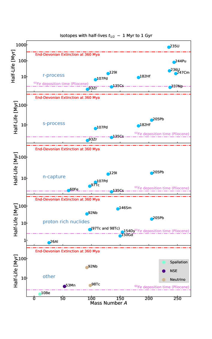
Figure 1: Radioisotopes with half-lives of interest to searches for nearby SN and KN explosions. The horizontal orchid-colored lines indicate the age of the SN explosion $\sim 3$ Mya attested by discoveries of deposits of ${}^{60}{\rm Fe}$, and the horizontal red lines mark the end-Devonian time scale. These five panels represent different nucleosynthesis channels, with the proton-rich nuclide panel including both $p$-process and $\gamma$-process isotopes, which are ordered by isotope mass number $A$.

Table 1: Radioisotopes with Half-lives $t_{1/2}\sim 1\ \rm Myr$ to ${\rm 1\ \rm Gyr}$: Astrophysical Production and Geological Detection

Isotope	Half-Life	Decay	Nucleosynthesis	AMS	Background	Notes on Extrasolar Evidence
	(Myr)	Mode	Process (Lug18)	(Kut13)	Measured	and Terrestrial Backgrounds (Section 3)
${}^{10}{\rm Be}$	1.51∗	$\beta^{-}$	CR (Gos01,Mas99)	yes	yes	used as chronometer
${}^{26}{\rm Al}$	0.717	$\beta^{+}$, EC	proton capture	yes	yes	searches in Fe-Mn crusts
${}^{53}{\rm Mn}$	3.74	EC	NSE	yes	yes	evidence in Fe-Mn crusts (Kor20)
${}^{60}{\rm Fe}$	2.62	$\beta^{-}$	neutron capture	yes	no	detection in Fe-Mn crusts and nodules, deep-ocean
						sediments, Antarctic snow, lunar regolith, cosmic rays
${}^{92}{\rm Nb}$	34.7	$\beta^{+}$	$\alpha$-rich freeze-out, $p$, $\nu$	yes (Guo13)	no
${}^{93}{\rm Zr}$	1.61	$\beta^{-}$	$s$ (She20), $r$,	yes	no
			$\alpha$-rich freeze-out
${}^{97}{\rm Tc}$	4.2	EC	$p$ (Nis18), $n$ capture	no	no	possible SN $\nu$ production in Mo ore (Hax88,Ngu05)
${}^{98}{\rm Tc}$	4.2	$\beta^{-}$	$p$ (Nis18), $\nu$ (Hay18)	no	no	possible SN $\nu$ production in Mo ore (Hax88,Ngu05)
${}^{107}{\rm Pd}$	6.5	$\beta^{-}$	$s$, $r$, $n$ capture	yes	no
${}^{129}{\rm I}$	15.7∗	$\beta^{-}$	$r$ (Dil08,Dav19)	yes	yes	pre-anthropogenic background seen in Fe-Mn crusts
			$n$ capture
${}^{135}{\rm Cs}$	1.33	$\beta^{-}$	$s$, $r$, $n$ capture	yes	no
${}^{146}{\rm Sm}$	68	$\alpha$	$p$ (Nis18)	yes	no
${}^{150}{\rm Gd}$	1.79	$\alpha$	$p$ (How93)	no	no
${}^{154}{\rm Dy}$	3.0	$\alpha$	$p$	no	no
${}^{182}{\rm Hf}$	8.9	$\beta^{-}$	$s$, $r$ (Voc04), $n$ capture	yes	no
${}^{205}{\rm Pb}$	17.3	EC	$s$, $n$ capture	yes	no
${}^{235}{\rm U}$	704	$\alpha$	$r$	yes	yes	high natural background
${}^{236}{\rm U}$	23.4	$\alpha$	$r$	yes	yes	natural and anthropogenic background
${}^{237}{\rm Np}$	2.14	$\alpha$	$r$	yes	yes	anthropogenic background seen
${}^{244}{\rm Pu}$	80∗	$\alpha$ 99.88%	$r$	yes	yes	detection in Fe-Mn crusts
		SF 0.12%				anthropogenic signature from global fallout (Ste13)
${}^{247}{\rm Cm}$	15.6	$\alpha$	$r$	yes	no	possible anthropogenic background

Notes:

Our calculations use half-lives from NUBASE2016 (Audi et al., 2017) as implemented in Mumpower et al. (2018) and Sprouse et al. (2020). As indicated by asterisks, the recent NUBASE2020 update (Kondev et al., 2021) has small changes to some values, including those of the r-process species ${}^{129}{\rm I}$ and ${}^{244}{\rm Pu}$.

Decay mode: $\beta^{-}$ = $\beta$-decay, $\beta^{+}$ = positron emission, EC = electron capture, $\alpha$ = $\alpha$-decay, SF = spontaneous fission

Nucleosynthesis process: CR = cosmic-ray spallation; NSE = nuclear statistical equilibrium; $s$ = weak/limited or main slow neutron capture ($s$) process; $p$ = $p$-process, synthesis of $p$-rich species by proton capture and/or $\gamma$-processes, $\nu$ = neutrino ($\nu$) process; $r$ = weak/limited or main rapid neutron capture ($r$) process; and $n$ capture = neutron captures on preexisting species.

AMS: Accelerator mass spectrometry demonstrated for this isotope.

Background measured: Natural or anthropogenic levels detected.

References: [Dav19] Davila et al. (2019), [Dil08] Dillmann (2008), [Gos01] Gosse & Phillips (2001), [Guo13] Guozhu et al. (2013), [Hax88] Haxton & Johnson (1988), [Hay18] Hayakawa et al. (2018), [How93] Howard (1993), [Kor20] Korschinek et al. (2020), [Kut13] Kutschera (2013), [Lug18] Lugaro et al. (2018), [Mas99] Masarik & Beer (1999), [Ngu05] McGary & Johnson (2007), [Nis18] Nishimura et al. (2018), [She20] Shetye et al. (2020), [Ste13] Steier et al. (2013), and [Voc04] Vockenhuber et al. (2004).

We now discuss relevant features of the various isotopes listed in Table 1. As noted, there is a large background of ${}^{10}{\rm Be}$ production by cosmic-ray interactions, so this is not a promising signature of a nearby astrophysical explosion. There is expected to be copious ejection of ${}^{53}{\rm Mn}$ and ${}^{60}{\rm Fe}$ by Type-Ia (Lugaro et al., 2018; Kobayashi et al., 2020) and core-collapse SNe, respectively, rather than by the $r$-process, and these isotopes are not expected to be prominent in KN debris. The main mechanism for producing the proton-rich isotopes ${}^{92}{\rm Nb}$ and ^97,${}^{98}{\rm Tc}$ is expected to be the $p$-process,  while there may be $p$-, $r$- and $s$-process contributions to ${}^{93}{\rm Zr}$ production. Most of the heavier isotopes with $A>100$ are expected to be produced mainly via the $r$-process, exceptions being ${}^{146}{\rm Sm}$, ${}^{150}{\rm Gd}$, ${}^{154}{\rm Dy}$ and ${}^{205}{\rm Pb}$.  In the cases of the actinide isotopes, one must be mindful of the possible presence of terrestrial anthropogenic contamination by nuclear accidents or bomb debris, which was an issue for the analysis of ${}^{236}{\rm U}$ and ${}^{237}{\rm Np}$ in Apollo lunar regolith samples (Fields et al., 1972, 1976). The ambient terrestrial level of ${}^{244}{\rm Pu}$ has been measured in Winkler et al. (2004), and the detection of ${}^{244}{\rm Pu}$ in deep-ocean deposits by Wallner et al. (2015) is thought to be free of this background, which was considered in detail in Wallner et al. (2021).

We focus in the following on the long-lived radioisotopes that could be synthesized through the $r$ process, as listed in the top panel of Fig. 1, and their production by SNe and KNe alongside ${}^{244}{\rm Pu}$. Since several of these isotopes have multiple avenues of astrophysical production while ${}^{244}{\rm Pu}$ is an $r$-only species, we emphasize that the $r$-process production ratios we present in the following are lower limits.

3 Searches for Explosion Ejecta on the Earth and Moon

The Earth and the Moon serve as natural archives that store any debris from nearby explosions that reach within 1 au from the Sun. This provides a great opportunity to bring samples of ejecta to the laboratory and analyze their content, which can be realized after finding suitable deposition sites and favorable samples by then identifying the signals within them. Live radioisotopes have the advantage of minimizing the natural background, which may render the search possible, even if the measurements remain difficult. As noted in Eqs. (1) - (3) and the surrounding discussion, the three timescales of particular interest are $\sim(3,50,and360)\ \rm Mya$, corresponding to the best-observed ${}^{60}{\rm Fe}$ pulse, the ${}^{244}{\rm Pu}$ half-life (approximately), and the end of the Devonian epoch.

3.1 Sensitivities to Radioisotopes of Interest

A challenge common to terrestrial and lunar searches is the tiny abundance of any radioisotope that one may wish to seek. The widespread ${}^{60}{\rm Fe}$ detections summarized in the introduction provide a model for successful detection of an extraterrestrial species. As discussed above, the $r$-process components of any reasonable signal are expected to have fluences smaller than the established ${}^{60}{\rm Fe}$ signal, implying that only AMS techniques may have the needed sensitivity, i.e., the capability of separating and identifying the isotopes of interest given the expected number of atoms per gram in a sample. At present, ${}^{60}{\rm Fe}$ measurements can find isotope fractions with a sensitivity down to $\mbox{${}^{60}{\rm Fe}$}/{\rm Fe}\sim(0.3-1)\times 10^{-16}$ (Wallner et al., 2020). However, this sensitivity may be impaired in the cases of isotopes with a significant cosmic-ray-induced background. For example, in the case of the recently reported evidence for the terrestrial deposition of ${}^{53}{\rm Mn}$, the apparent excess of the signal over the background is $\mbox{${}^{53}{\rm Mn}$}/{\rm Mn}\sim 1.5\times 10^{-14}$ (Korschinek et al., 2020). 

When a natural terrestrial background is absent or small, AMS sensitivities are often limited by the ability to remove or discriminate an interfering stable isobar with the same $A$ and thus nearly the same mass as the species of interest; this is important for many of the r-process signals that may reside within these samples. Removal of this interference is typically performed through both chemical processing and ion identification techniques, but limitations still remain. Recent advances suggest that it is possible to reach $\mbox{${}^{93}{\rm Zr}$}/\mbox{${}^{92}{\rm Zr}$}\sim 6\times 10^{-11}$ (Hain et al., 2018; Pavetich et al., 2019), though this hinges on successful removal of the stable isobar ${}^{93}{\rm Nb}$. In the case of ${}^{107}{\rm Pd}$, Korschinek et al. (1994) reported an AMS sensitivity $\mbox{${}^{107}{\rm Pd}$}/\mbox{${}^{106}{\rm Pd}$}\sim 10^{-8}$; here the interfering stable isobar is ${}^{107}{\rm Ag}$. In the case of ${}^{129}{\rm I}$ there is a natural background level $\mbox{${}^{129}{\rm I}$}/\mbox{${}^{127}{\rm I}$}\sim 1.5\times 10^{-12}$ (Ji et al., 2015b). Sensitivities down to $\mbox{${}^{129}{\rm I}$}/\mbox{${}^{127}{\rm I}$}\lesssim 10^{-14}$ are possible (Vockenhuber et al., 2015) since the interfering stable isobar ${}^{129}{\rm Xe}$ is an inert gas, fortuitously, so it does not form negative ions and will not interfere. In the case of ${}^{135}{\rm Cs}$, Yin et al. (2015) were able to reduce stable isobar contamination to $\mbox{${}^{135}{\rm Ba}$}/\mbox{${}^{133}{\rm Cs}$}\sim 9\times 10^{-12}$, and we adopt the same value for the prospective sensitivity to ${}^{135}{\rm Cs}$, namely $\mbox{${}^{135}{\rm Cs}$}/\mbox{${}^{133}{\rm Cs}$}\sim 9\times 10^{-12}$. In the case of ${}^{182}{\rm Hf}$, Vockenhuber et al. (2004) reported a sensitivity $(\mbox{${}^{182}{\rm Hf}$}+{\mbox{${}^{182}{\rm W}$}})/\mbox{${}^{180}{\rm Hf}$}\sim 10^{-11}$; the ability to measure $\mbox{${}^{182}{\rm Hf}$}/\mbox{${}^{180}{\rm Hf}$}$ to this precision or better requires that techniques be developed to suppress further the stable isobar ${}^{182}{\rm W}$. In the case of ${}^{236}{\rm U}$, there are no isobaric contaminants, and the detection limits are set by the ability to discriminate the neighboring abundant uranium isotopes ${}^{235}{\rm U}$ and ${}^{238}{\rm U}$. Efforts by Wilcken et al. (2008) estimate a detection limit of ${}^{236}{\rm U}$/${}^{238}{\rm U}$ $\sim 10^{-13}$.

In the cases of ${}^{237}{\rm Np}$, ${}^{244}{\rm Pu}$, and ${}^{247}{\rm Cm}$, there are no stable isotopes nor isobars, so searches can first focus simply on extracting the element, guarding against anthropogenic contamination, which could be orders of magnitude greater than a stellar signal (Wallner et al., 2004). In addition, these AMS samples must be “spiked” with a known quantity of shorter-lived isotopes of each species in order to calibrate the response. Both ${}^{236}{\rm Pu}$ and ${}^{242}{\rm Pu}$ have been used as calibration standards for ${}^{244}{\rm Pu}$ (Wallner et al., 2004; Raisbeck et al., 2007; Wallner et al., 2015). The other species have been studied less. In the case of ${}^{237}{\rm Np}$, sector-field inductively coupled plasma mass spectrometry studies have sensitivities down to a mass fraction of $10^{-15}$ within soil and sediment samples (Röllin et al., 2009), while systematic AMS studies suggest subfemtogram-per-sample detection limits as long as the ${}^{238}{\rm U}$ content remains sufficiently low  (Fifield et al., 1997; López-Lora & Chamizo, 2019). Initial AMS studies of ${}^{247}{\rm Cm}$ made by Christl et al. (2014) suggest a detection limit of $<$0.1 femtogram in a typical sample, where limits were set by the impurities of the ${}^{244}{\rm Cm}$ spike added for reference.

3.2 Plutonium Measurements

We anchor our predictions for prospective $r$-process radioisotopes using the results of geological searches for ${}^{244}{\rm Pu}$ in deep-ocean crusts and sediments that are displayed in Fig. 2 and are summarized in Table 2.  The most significant of these is the remarkable Wallner et al. (2021) study, which not only presented solid detections of astrophysical ${}^{244}{\rm Pu}$ in an Fe-Mn crust from the deep Pacific, but also identified the two ${}^{60}{\rm Fe}$ peaks.

Any claim of astrophysical ${}^{244}{\rm Pu}$ detection must contend with anthropogenic contamination, and this is a major focus of Wallner et al. (2021). They searched not only for ${}^{244}{\rm Pu}$, which potentially contains an astrophysical signal, but also for the short-lived ${}^{239}{\rm Pu}$, ${}^{240}{\rm Pu}$, and ${}^{241}{\rm Pu}$ isotopes, which measure anthropogenic contamination. All of the ${}^{239}{\rm Pu}$, ${}^{240}{\rm Pu}$ and ${}^{241}{\rm Pu}$ were found in the top layers of the crust, and exhibited ${}^{239}{\rm Pu}$/${}^{240}{\rm Pu}$ and ${}^{239}{\rm Pu}$/${}^{241}{\rm Pu}$ ratios consistent with anthropogenic fallout. This shows that some uptake has occurred in modern times. In the deeper layers corresponding to times ${\cal O}$(several) Mya, the ${}^{244}{\rm Pu}$/${}^{239}{\rm Pu}$ ratio shows an excess over the value in the top layer. In contrast, the ${}^{240}{\rm Pu}$/${}^{239}{\rm Pu}$ and ${}^{241}{\rm Pu}$/${}^{239}{\rm Pu}$ ratios do not show significant variation with depth. The fact that, uniquely, ${}^{244}{\rm Pu}$ exhibits an excess points to a source for this isotope distinct from anthropogenic production. There being no significant natural ${}^{244}{\rm Pu}$ on Earth today, the signal must be extraterrestrial.

Wallner et al. (2021) inferred the extraterrestrial ${}^{244}{\rm Pu}$ incorporation rate into the crust, after subtracting the anthropogenic ${}^{244}{\rm Pu}$ contribution. An incorporation efficiency or uptake of $U_{\rm Pu}=0.17$ is adopted, the same as that found for ${}^{60}{\rm Fe}$ in the same crust. For the two layers below the top, fluxes are evaluated as follows (see also Table 2):

$$\Phi_{244}^{\rm interstellar}(0-4.76\ \rm Myr) = (1.67\pm 0.35)\times 10^{3}\ \rm atoms\ cm^{-2}\ Myr^{-1}\,,$$ (4)

$$\Phi_{244}^{\rm interstellar}(0-9\ \rm Myr) = (0.98\pm 0.18)\times 10^{3}\ \rm atoms\ cm^{-2}\ Myr^{-1}\,.$$ (5)

These fluxes will be central inputs to our study. We see that these timespans overlap with the ${}^{60}{\rm Fe}$ pulses at $\sim 3$ and $\sim 7$ Myr ago. These data leave open the question of whether the flux is different in the earlier time bin versus the overall average; the reported difference of about $1.8\sigma$ is not decisive.

Other important ${}^{244}{\rm Pu}$ measurements have been reported previously. An upper limit of $\Phi_{244}^{\rm interstellar}<2\times 10^{5}\ \rm atoms\ cm^{-2}\ Myr^{-1}$ on the rate of extraterrestrial deposition in young sediment was set by Paul et al. (2001). Subsequently, AMS measurements of crust VA13-2 by Wallner et al. (2004) and of sediment MD90-0940 by Raisbeck et al. (2007) each yielded one event, dated to $1-14$ Mya and $2.4-2.7$ Mya, respectively. Raisbeck et al. (2007) did not attribute their single event to a signal, but derived upper limits on the fluence assuming one count in each of three time bins. We follow this practice, noting that the flux inferred from the nonzero bin would vastly exceed the other limits and detections overlapping this time period. More recently, a search for ${}^{244}{\rm Pu}$ by Wallner et al. (2015) yielded a possible signal in three samples corresponding to three different epochs: sediments spanning $0.53-2.17$ Mya, and crust layers at $5-12$ Mya and $12-25$ Mya. In each of these samples, at most only a single ${}^{244}{\rm Pu}$ count was found in each time bin, so these results must be treated with great caution.

Figure 2: Geological searches for ${}^{244}{\rm Pu}$, in deep-ocean crusts (Wallner et al., 2004, 2015) and sediments (Paul et al., 2001; Raisbeck et al., 2007; Wallner et al., 2015). The ${}^{244}{\rm Pu}$ flux is

expressed as a measurement when the count is nonzero, and as a limit for zero counts and for the first (Raisbeck et al., 2007) time bin as described in the text.

Table 2: Geological Searches for Natural ${}^{244}{\rm Pu}$

Study	Sample	Time	${}^{244}{\rm Pu}$ Counts	Flux $\Phi_{244}^{\rm interstellar}$	Fluence ${\cal F}_{244}^{\rm interstellar}$
		[Mya]	[atoms]	$[\rm atoms\ cm^{-2}\,Myr^{-1}]$	$[\rm atoms\ cm^{-2}]$
Paul et al. (2001)	Sediment 92SAD01	$0-0.3$	$1^{*}$	$<2\times 10^{5}$	$<2\times 10^{4}$
Wallner et al. (2004)	Crust VA13-2	1–14	1	2500	$1.6\times 10^{4}$
Raisbeck et al. (2007)	Sediment MD90-0940	2.4–2.7	1	$<3\times 10^{7}$	$<3\times 10^{6}$
Wallner et al. (2015)	Crust 273KD	0.5–5	0	$<3500$	$<800$
		5–12	1	$247_{-235}^{+1000}$
		12–25	1	$320_{-300}^{+1250}$
	Sediment TR149-217	0.53–2.17	1	$3000_{-850}^{+12000}$
Wallner et al. (2021)	Crust-3/A	0 - 1.34	$34\pm 17$	$930\pm 480$	$1200\pm 600$
	Crust-3/B	1.34 - 4.57	$141\pm 19$	$1990\pm 440$	$6400\pm 1400$
	Crust-3/C	4.57 - 9.0	$6.3^{+4.3}_{-3.2}$	$270^{+180}_{-140}$	$1200^{+800}_{-600}$

^∗Paul et al. (2001) argue that their detection could be due to anthropogenic contamination.

The detections reported in Fig. 2 and Table 2 show that extraterrestrial ${}^{244}{\rm Pu}$ deposition has occurred over at least over the last 9 Myr and possibly goes back to as far as 25 Myr. Taking the measurements at face value, it would seem that the ${}^{244}{\rm Pu}$ flux history differs from the two ${}^{60}{\rm Fe}$ pulses, which are each limited in time (though a small ${}^{60}{\rm Fe}$ continues to the present). That is, the wide time ranges of the Wallner et al. (2021) detections both overlap with the ${}^{60}{\rm Fe}$ pulses, but earlier indications of ${}^{244}{\rm Pu}$ flux extend from nearly the present back to at least 12 to 25 Mya. Within the large uncertainties, it is unclear if the flux varies over this time. The data could accommodate–but within uncertainties do not demand–a larger flux around the time of the ${}^{60}{\rm Fe}$ pulse(s) at $\sim 3$ Mya (and $\sim 7$ Mya). The possible difference between the ${}^{60}{\rm Fe}$ and ${}^{244}{\rm Pu}$ deposition histories suggests a different origin for at least some of the ${}^{244}{\rm Pu}$, a point also made in previous studies, e.g., Wallner et al. (2015).

4 Modeling $r$-Process Production in SNe and KNe

We can link the observed ${}^{244}{\rm Pu}$ flux with that of other r-process radioisotopes through theoretical calculations of r-process nucleosynthesis. These calculations depend on the nature of the candidate nucleosynthesis event, and on the nuclear inputs one adopts. The results are constrained by the observed r-process pattern in solar system material and in stars. Here we describe our calculations and their uncertainties.

The production ratios of radioactive isotopes resulting from an $r$-process event can be estimated by the extraction and post-processing of ejected matter trajectories from astrophysical simulations of the event. The trajectories contain the time history of $(\rho,T,andY_{e})$, where $\rho$ is the density, $T$ is the temperature, and the electron fraction $Y_{e}=n_{e}/n_{B}=\langle Z/A\rangle$ measures the neutron richness $Y_{n}=1-Y_{e}=\langle N/A\rangle$. The evolution of the nuclear material along this trajectory is then calculated using a network of the relevant nuclear reactions. This procedure brings with it significant challenges, starting from the identification and characterization of the appropriate nucleosynthesis sites within the candidate event.

SNe were the first type of event suggested for $r$-process production (Burbidge et al., 1957), and for many decades the core-collapse SN neutrino-driven wind was considered the leading candidate site. However, modern simulations show that the neutrino-driven wind is unlikely to be sufficiently neutron-rich to synthesize the actinides (Fischer et al., 2010; Hüdepohl et al., 2010; Arcones & Thielemann, 2013), though it may produce $A\sim 80$-100 species through a weak $r$-process (Bliss et al., 2018) or a $\nu p$-process (Fröhlich et al., 2006). The ultimate extent of nucleosynthesis in this environment depends on neutrino physics that is not fully understood (Balantekin & Yüksel, 2005; Duan et al., 2011; Johns et al., 2020; Xiong et al., 2020). Rare types of core-collapse events may also generate neutron-rich outflows, with promising candidates including magneto-rotational (MHD) SNe (Winteler et al., 2012; Mösta et al., 2018; Reichert et al., 2021) and collapsars (Pruet et al., 2003; Surman et al., 2006; Fujimoto et al., 2008; Siegel et al., 2019).

Studies of galactic chemical evolution suggest that, whilst collapsars might have been important early in the history of the universe during the epoch of Population III stars, they were less relevant during the epochs of interest for this study. For this reason, and given the uncertainty in how robust collapsar $r$-process calculations might be (Miller et al., 2020), we do not consider them further in this paper. 

While neutron star mergers have recently been confirmed to produce $r$-process elements (Cowperthwaite et al., 2017; Kasen et al., 2017; Abbott et al., 2017; Abbott et al., 2017), exactly how, where, and how much have yet to be definitively worked out (see reviews in Cowan et al., 1991; Arnould et al., 2007; Kajino et al., 2019; Cowan et al., 2021, and references therein). Possible nucleosynthetic environments within a merger include the prompt ejecta—cold, very neutron-rich tidal tails and/or shock-heated ejecta from the neutron star contact interface (Bauswein et al., 2013; Hotokezaka et al., 2013; Rosswog et al., 2013; Endrizzi et al., 2016; Lehner et al., 2016; Sekiguchi et al., 2016; Rosswog et al., 2017)—and magnetic, viscous, and/or neutrino-driven outflows from the resulting accretion disk (Chen & Beloborodov, 2007; Surman et al., 2008; Dessart et al., 2009; Perego et al., 2014; Wanajo et al., 2014; Just et al., 2015; Martin et al., 2015; Siegel & Metzger, 2018). The composition and relative contributions of each type of mass ejection depend on quantities such as the physical parameters of the merging system and the still unknown microphysics of dense matter and its neutrino emission (see, e.g., Caballero et al., 2012; Foucart et al., 2015; Malkus et al., 2016; Kyutoku et al., 2018).

In view of the large astrophysical uncertainties in each candidate $r$-process site, our calculations of isotopic yields rely on illustrative models that indicate the ranges of possibilities. We choose matter trajectories from modern simulations that capture the rough characteristics ($Y_{e}$, entropy $s/k$, and dynamical timescale $\tau$) expected for each site. Different combinations of ($Y_{e}$, $s/k$, and $\tau$) lead to distinct nucleosynthetic pathways through the neutron-rich side of the nuclear chart, leading to different amounts of individual isotopes even when the final elemental yields are similar. We choose at least two distinct trajectories for each type of event so as to ensure production of both main ($A>120$) and weak ($70<A<120$) $r$-process nuclei.

We adopt four illustrative $r$-process model combinations, using trajectories from a forced modification of a conventional SN neutrino-driven wind scenario (SA), an MHD SN model (SB), and two neutron star merger disk and dynamical ejecta combinations (KA and KB). We then combine and scale the resulting abundances to the elemental patterns of select $r$-process-enhanced stars. We scale to individual metal-poor stars rather than, e.g., the solar abundances, since these stars have experienced fewer generations of stellar nucleosynthesis and thus are cleaner representations of the yields from single $r$-process events. We choose one of the few stars for which elements in all three $r$-process peaks have been detected  (Roederer & Lawler, 2012), and J0954+5246, the star with the largest enhancement in actinide elements ever detected (Holmbeck et al., 2018). We use a variety of $r$-process species measured in the above-discussed metal-poor stars to normalize our estimates, including ytterbium, tellurium, cadmium and zirconium, and note the mixing fraction(s) $f$ of the total mass(es) of the weak $r$-process trajectory (trajectories) relative to the most neutron-rich $r$-process trajectory that appears in the combined model fit. The total mass of the $r$-process ejecta for each model is normalized to unity. The details of each model combination and constraint are described below and summarized in Table 3.

Our nucleosynthesis calculations are made with the nuclear reaction network code Portable Routines for Integrated nucleoSynthesis Modeling (PRISM; Mumpower et al. (2018); Sprouse et al. (2020)), implemented as in  Wang et al. (2020b) for the baseline calculation. We note that isotopic ratio estimates are shaped in addition by the nuclear physics properties of the thousands of exotic nuclei that participate in an $r$-process. Thus for each model we explore variations in the nuclear inputs for quantities for which experimental values are unavailable (masses from Goriely et al. (2009) (HFB), or $\beta$-decay rates from Marketin et al. (2016) (MKT) for both SN and KN models, and fission yields from Kodama & Takahashi (1975) for KN models), as in Wang et al. (2020a). Additionally, because of the general limitation of the network code for time step evolution at times $\gtrsim$ Myr, which results in large time steps comparable to the half-lives of the radioisotopes of interest in this work such as ${}^{93}{\rm Zr}$, we use PRISM to generate $r$-process abundance yields until 1 kyr for ${}^{182}{\rm Hf}$ and lighter radioisotopes, and until 1 Myr for actinides (except for ${}^{248}{\rm Cm}$ and ${}^{245}{\rm Cm}$, for which we run until 0.1 Myr), and then switch to a pure radioactive decay calculation for these radioisotopes. These calculations provide the relative abundance yields for the radioisotopes.

As commented above, the SN neutrino-driven wind scenario has fallen out of favor as a primary $r$-process site because modern simulations do not show that sufficiently neutron-rich conditions to reproduce the solar r-process pattern (Fischer et al., 2010; Hüdepohl et al., 2010; Arcones & Thielemann, 2013). Indeed, no actinides are produced at all. We are however motivated by the intriguing possibility of coincident identifications of ${}^{60}{\rm Fe}$ and ${}^{244}{\rm Pu}$ to consider here a forced neutrino-driven wind scenario, denoted in Table 3 by ”$\nu\star$”. We start with the neutrino-driven wind simulations of Arcones et al. (2007); Arcones & Janka (2011) and modify the initial $Y_{e}$ in order to produce different $r$-process yields. The upper panel of Fig. 3 shows the final abundance pattern results at $t\sim 10\ \rm Gyr$ for four values of $Y_{e}=0.31$ (blue), 0.35 (yellow), 0.42 (green), and 0.48 (pink). We have found that results for $Y_{e}\leq 0.31$, following different trajectories, and using different nuclear networks, make qualitatively similar predictions for substantial production of isotopes with atomic numbers $A\gtrsim 130$, up to and including the actinides. On the other hand, simulations with $Y_{e}\geq 0.38$ yield much less production of isotopes with $A\gtrsim 130$, as exemplified by the results shown in green and pink. The results shown in red are for a mixture (model SA) of the simulations for SN forced neutrino-driven wind with four different values of $Y_{e}$ (see Table 3), whose relative normalizations are scaled to fit data on the abundances of ytterbium, tellurium, cadmium, and zirconium in the metal-poor star HD 160617 (Roederer & Lawler, 2012). The range of $Y_{e}$ in the SA model is similar to that of the SN model with actinide production in Goriely & Janka (2016). These and other abundances are shown in gray in the upper panel of Fig. 3, and we see in the lower panel of Fig. 3 that model SA also matches the solar abundance data very well.

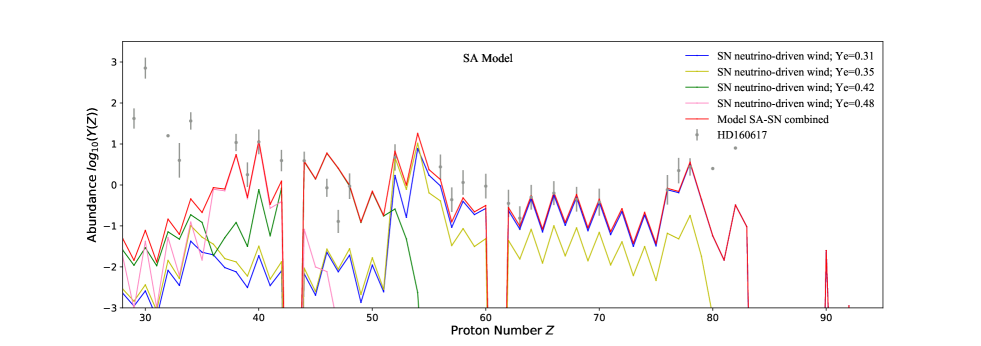
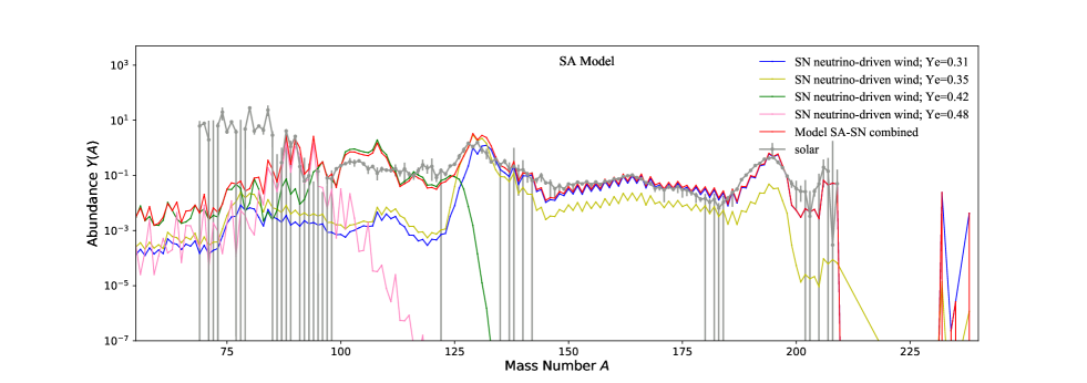
Figure 3: Upper panel: The abundances at $t\sim 10\ \rm Gyr$ of $r$-process nuclei produced in SN forced modifications of neutrino-driven wind simulations from Arcones et al. (2007) and Arcones & Janka (2011) with the electron fractions $Y_{e}=0.31$ (blue), $0.35$ (yellow), $0.42$ (green), and $0.48$ (pink), and a combination (SA, red) fitted to abundances measured in the metal-poor star HD 160617 (Roederer & Lawler, 2012), plotted as functions of the atomic number $Z$. Lower panel: A comparison with the corresponding solar abundance data (Arnould et al., 2007), plotted as functions of the atomic weight $A$.

	SN Models		KN Models
Label	SA ($\nu\star$)	SB (MHD)	KA	KB
Simulations	SN forced neutrino-driven wind: four trajectories	MHD SN:	KN dynamical ejecta: two trajectories from Bovard et al. (2017)
	from Arcones et al. (2007); Arcones & Janka (2011)	two trajectories from	diskwind: 2 trajectories from Just et al. (2015)
	with modified $Y_{e}=0.31,0.35,0.42,and0.48$	Mösta et al. (2018)
Scaling	HD 160617: Yb, Te, Cd and Zr	HD 160617: Yb and Zr	HD 160617: Yb and Zr	J0954+5246: Yb and Zr
Mixing fractions $f$	$f_{0.35}$=0.757, $f_{0.42}$=1.778, and $f_{0.48}$=0.770	3.137	3.980	0.819

Table 3: Combinations of Forced Modifications of Neutrino-driven SN Models (Arcones et al., 2007; Arcones & Janka, 2011) and MHD Models (Mösta et al., 2018) Constrained by Observations of the Metal-poor Star HD160617 (Roederer & Lawler, 2012) (SA and SB, Respectively), and Combinations of KN Dynamical Ejecta Models (Bovard et al., 2017) with Disk Neutrino-driven Wind Models from Just et al. (2015), Constrained by Observations of HD160617 (KA) or the Actinide-boost star J0954+5246 (Holmbeck et al., 2018) (KB).

Fig. 4 shows analogous results using the Mösta et al. (2018) MHD SN model. In the upper panel, we show the abundance predictions of two trajectories (blue for the main r-process trajectory and green for the light r-process trajectory) and a combination (SB, red) fitted to the abundances of ytterbium and zirconium measured in the metal-poor star HD 160617 (Roederer & Lawler, 2012) (see Table 3). These and other abundances are shown in gray in the upper panel of Fig. 4, and we see in the lower panel of Fig. 4 that this mixture of simulations also matches the solar abundance data quite well in general, though it overestimates the structure seen in the solar data for $A\sim 130$, and falls off more rapidly for $A\gtrsim 190$. Indeed, almost all modern SN models struggle to produce actinides, displaying higher production of lighter $r$-process species relative to plutonium as described in the next section.

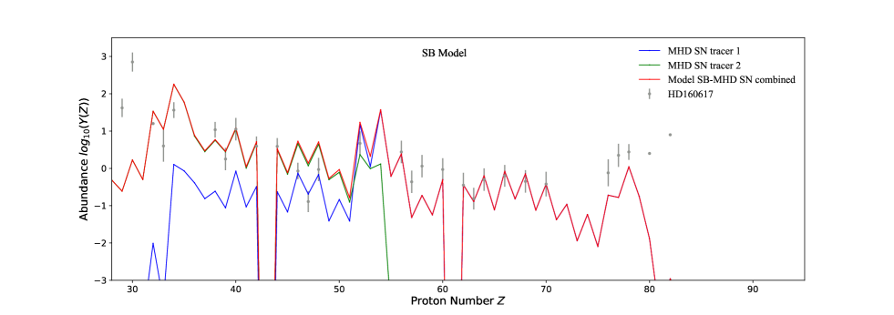
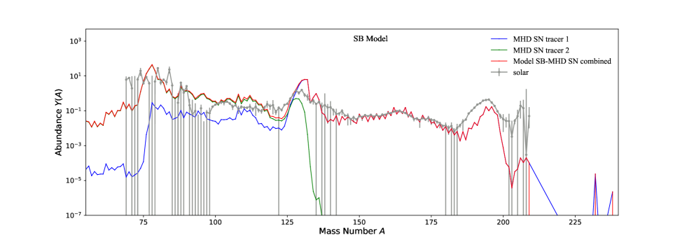
Figure 4: Upper panel: The abundances at $t\sim 10\ \rm Gyr$ of $r$-process nuclei produced in MHD SN simulations from Mösta et al. (2018) with two different tracers 1 (blue) and 2 (green) and a combination (SB, red) fitted to the abundances of ytterbium and zirconium measured in the metal-poor star HD 160617 (Roederer & Lawler, 2012), plotted as functions of the atomic number $Z$. Lower panel: A comparison with the corresponding solar abundance data (Arnould et al., 2007), plotted as functions of the atomic weight $A$.

The upper panel of Fig. 5 shows results from representative simulations of the abundances of nuclei produced by the $r$-process (at $t\sim 10$ Gyr) in KN dynamical ejecta based on the work of Bovard et al. (2017) (blue), and in KN disk neutrino-driven wind based on the work of Just et al. (2015) (green). Also shown is a combination of these simulations (KA, red) fitted to the abundances of ytterbium and zirconium in the metal-poor star HD 160617 (Roederer & Lawler, 2012) (see Table 3). These and other abundances are shown in gray in the upper panel of Fig. 5, and we see in the lower panel of Fig. 5 that the KA model also matches the solar abundance data quite well, though with some deviations for $A\sim 140$.

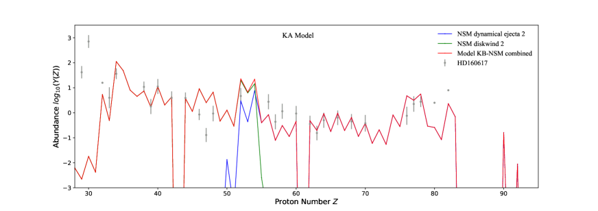
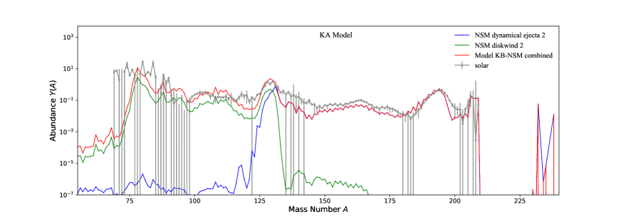
Figure 5: Upper panel: The abundances at $t\sim 10\ \rm Gyr$ of $r$-process nuclei produced in simulations of KN dynamical ejecta from Bovard et al. (2017) (blue) and of disk neutrino-driven wind from Just et al. (2015) (green), and a mixture (KA, red) fitted to measurements of the metal-poor star HD 160617 (Roederer & Lawler, 2012), plotted as functions of the atomic number $Z$. Lower panel: The corresponding abundance pattern of model KA compared with solar abundance data (Arnould et al., 2007), plotted as functions of the atomic weight $A$.

As compared with Figure. 5, Figure. 6 shows analogous results obtained using the KN dynamical model with a relatively more neutron-rich trajectory from Bovard et al. (2017) (blue), and the disk neutrino-driven wind model of Just et al. (2015). Also shown are the predictions of a combination (KB, red) fitted to the abundances of ytterbium and zirconium measured in the actinide-boost star J0954+5346 (Holmbeck et al., 2018). These and other abundances are shown in gray in the upper panel of Fig. 6, and we see in the lower panel of Fig. 6 that this combination model also matches the solar abundance data quite well in general, though with some deviations from the solar data for $A\sim 120$ and $A\sim 135$. The KA and KB models both exhibit robust production of actinides that subsequently fission, so fission yields play important roles in shaping the second peak in these models (Eichler et al., 2015; Giuliani et al., 2020; Vassh et al., 2019, 2020). The fission yields of most neutron-rich actinides have not been experimentally determined, so in addition to the simple symmetric-split fission yields adopted in the baseline calculation, we also implement the wide-Gaussian fission yields from Kodama & Takahashi (1975) to estimate the uncertainty range. We find that the fission yields from Kodama & Takahashi (1975) would bring a small boost to the left and right sides of the second peak ($A\sim 120$ and $A\sim 133$) for the KA model, while leaving the yields of the interesting $r$-process radioisotopes listed in Table 5 largely unchanged. For the KB model with boosted actinide production, fission deposition could potentially fill the gap around $A\sim 120$ and lower the bump around $A\sim 133$ to bring the abundance pattern closer to the solar pattern, thus resulting in a smaller ${}^{135}{\rm Cs}$ yield. In a more extreme example of a wider distribution of fission fragments, the neutron star merger nucleosynthesis calculations in Shibagaki et al. (2016) exhibit a fission-recycling $r$-process pattern without a second peak, which could bring even smaller abundance yields of ¹²⁹I and ${}^{135}{\rm Cs}$. Additionally, spallation reactions that can occur when fast neutron star merger ejecta interact with the ISM may also affect the abundances of the radioisotopes located around $r$-process peaks (Wang et al., 2020a). These details do not influence the overall conclusion, however, that the KN models are predicted to produce actinides robustly, leading to lower ratios of lighter $r$-process species relative to plutonium, as described in the next section.

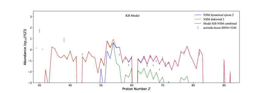
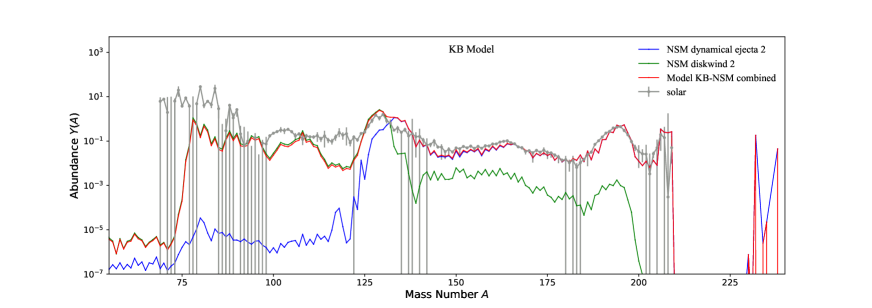
Figure 6: Upper panel: The abundances (at $t\sim 10Gyr$) of $r$-process nuclei produced in simulations of KN more neutron-rich dynamical ejecta from Bovard et al. (2017) (blue) and of disk neutrino-driven wind from Just et al. (2015) (green), and a mixture (KB, red) fitted to the measurements of the actinide-boost star J0954+5346 (Holmbeck et al., 2018), plotted as functions of the atomic number $Z$. Lower panel: The corresponding abundance pattern of model KB compared with solar abundance data (Arnould et al., 2007), plotted as functions of the atomic weight $A$.

5 $r$-Process Radioisotope Ratios and Time Evolution

We have already seen in Figs. 3, 4,  5, and 6 that the abundances of different $r$-process radioisotopes depend sensitively on the model of the SN or KN that is adopted. The same holds for actinide isotopes, even when attention is focused on hybrid models whose parameters are adjusted to yield ratios of the radioisotopes with $A\lesssim 200$ that are similar to those measured for the metal-poor star HD 160617 or the actinide-boost star J0954+5346. Tables 4, 5, 6 and 7 show the production ratios for the $r$-process isotopes of interest after $10^{5}$ yr (i.e., after the decays of short-lived isotopes), 3 Myr (as in eq. 1, corresponding to the ${}^{60}{\rm Fe}$ detection from near the end of the Pliocene era: the ratios after 7 Myr corresponding to the other ${}^{60}{\rm Fe}$ pulse reported in Wallner et al. (2021) are similar), 50 Myr (as in eq. 2, comparable with the half-life of ${}^{244}{\rm Pu}$), and 360 Myr (eq. 3; the time since the end-Devonian mass extinction(s)), respectively, as discussed in Section 1. These have been calculated from the SN and KN models studied in the previous Section 4, and are expressed as the abundance ratios relative to ${}^{244}{\rm Pu}$. Included for information are the production ratios for several $r$-process isotopes with half-lives $>500$ Myr, namely ${}^{232}{\rm Th}$, ${}^{235}{\rm U}$, and ${}^{238}{\rm U}$. However, in view of the backgrounds from astrophysical processes before the formation of the solar system, we do not consider further these isotopes.

Also, we note that SNe in general produce ${}^{60}{\rm Fe}$ by other nuclear mechanisms in addition to the $r$-process, such as by explosive burning, where the yield is expected to exceed greatly any possible $r$-process contribution, so the ${}^{60}{\rm Fe}$/${}^{244}{\rm Pu}$ ratios for SN models SA and SB in these and subsequent tables are in general underestimates and could be viewed as lower limits on the actual ratio. If the ratio of the ${}^{60}{\rm Fe}$ synthesized through the $r$-process to the total ${}^{60}{\rm Fe}$ produced in a SN is $\sim f(\mbox{${}^{60}{\rm Fe}$},r)$, then the ${}^{60}{\rm Fe}$/${}^{244}{\rm Pu}$ ratio for the SN model is boosted to $Y(\mbox{${}^{60}{\rm Fe}$})/(f(\mbox{${}^{60}{\rm Fe}$},r)Y(\mbox{${}^{244}{\rm Pu}$}))$. Additionally, our SN models provide the estimates per $r$-process event ${Y_{i}}({\rm SN,r})$, implicitly assuming that all SNe are similar $r$-process sites. As only a small fraction of SNe may be $r$-process sites, we may account for SN heterogeneity by assuming, in the crudest picture, that the the $r$-process occurs in only a fraction $f_{\rm SN,r}$ of SNe. In this case, the probability that a given SN will eject $r$-process material is $f_{\rm SN,r}$, implying that, for the $r$-process yield per SN event, ${Y_{i}}({\rm SN})$ must be lower, i.e., ${Y_{i}}({\rm SN})={f_{\rm SN,r}}{Y_{i}}({\rm SN,r})$.

Table 4: r-Process Isotope Production Ratios after $10^{5}\ \rm yr$

Radioisotope	SN Model		KN Model
Ratio	SA	SB	KA	KB
${}^{60}{\rm Fe}$/${}^{244}{\rm Pu}$	0.39	$2.5\times 10^{4}$	$8.6\times 10^{-3}$	$4.5\times 10^{-5}$
${}^{93}{\rm Zr}$/${}^{244}{\rm Pu}$	35	$6.4\times 10^{5}$	28	1.1
${}^{107}{\rm Pd}$/${}^{244}{\rm Pu}$	$1.4\times 10^{2}$	$3.9\times 10^{5}$	18	1.8
${}^{129}{\rm I}$/${}^{244}{\rm Pu}$	$7.1\times 10^{2}$	$4.5\times 10^{6}$	$1.8\times 10^{2}$	41
${}^{135}{\rm Cs}$/${}^{244}{\rm Pu}$	48	$1.2\times 10^{6}$	2.6	13
${}^{182}{\rm Hf}$/${}^{244}{\rm Pu}$	7.5	$1.2\times 10^{4}$	1.5	0.28
${}^{232}{\rm Th}$/${}^{244}{\rm Pu}$	2.7	24	1.7	0.65
${}^{235}{\rm U}$/${}^{244}{\rm Pu}$	2.9	15	3.1	1.7
${}^{236}{\rm U}$/${}^{244}{\rm Pu}$	3.8	23	3.7	2.4
${}^{238}{\rm U}$/${}^{244}{\rm Pu}$	2.2	9.6	2.4	1.5
${}^{237}{\rm Np}$/${}^{244}{\rm Pu}$	3.3	8.9	3.4	2.6
${}^{242}{\rm Pu}$/${}^{244}{\rm Pu}$	1.9	2.6	1.9	1.9
${}^{247}{\rm Cm}$/${}^{244}{\rm Pu}$	1.1	1.2	0.97	1.0
${}^{248}{\rm Cm}$/${}^{244}{\rm Pu}$	1.1	1.5	0.86	1.1

Fig. 7 displays the subsequent time evolution of several radionuclides of interest (${}^{60}{\rm Fe}$, ${}^{93}{\rm Zr}$, ${}^{107}{\rm Pd}$, ${}^{129}{\rm I}$, ${}^{135}{\rm Cs}$, ${}^{182}{\rm Hf}$, ${}^{244}{\rm Pu}$ and ${}^{247}{\rm Cm}$) from an $r$-process event only as calculated using the SN and KN models discussed in the previous section. The solid lines are obtained using our baseline $r$-process calculation, and the shaded bands are the ranges that result from the nuclear data variations described in Section 4. Also shown as vertical lines are the three timescales of interest, namely the age of the well-attested SN explosion $\sim 3$ Mya, an age of $50$ Mya comparable with the half-life of ${}^{244}{\rm Pu}$, and the age of the end-Devonian extinction(s) $\sim 360$ Mya. We see that there are substantial differences between the abundances of the radioisotopes calculated in different models. We note that the relative production rates of light (second peak and lighter) and heavy (third peak and higher) $r$-process nuclei depend strongly on the astrophysical conditions of the $r$-process sites. On the other hand, the relative ratios of the actinides themselves are largely insensitive to the site and thus have less discriminating power. The uncertainties in the relative yields of the actinides are dominated by large nuclear physics uncertainties in this region, so their yields depend sensitively on the choice of nuclear data adopted (as seen in Figure 7). Therefore measurements of radioisotope ratios, especially the ratios of light $r$-process nuclei to actinides, could provide useful diagnostic tools for the nature of any astrophysical explosion that occurred near Earth within the last few hundred million years.

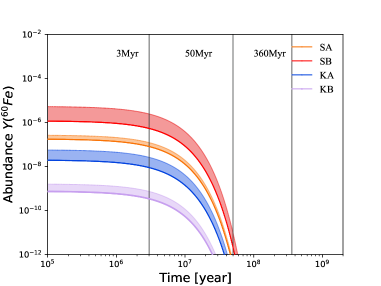
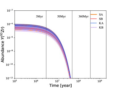
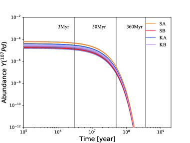
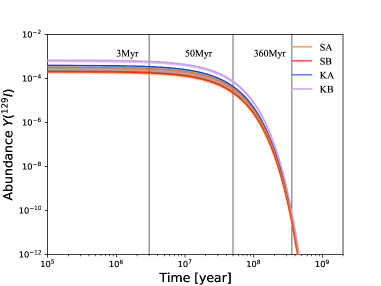
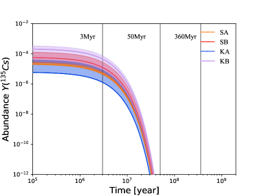
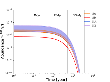
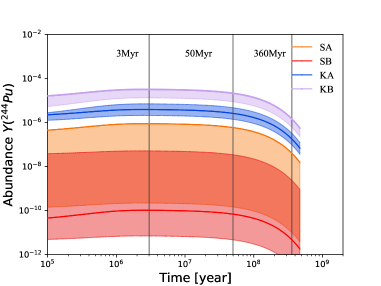
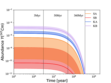
Figure 7: The time evolutions of the relative abundances of ${}^{60}{\rm Fe}$, ${}^{93}{\rm Zr}$, ${}^{107}{\rm Pd}$, ${}^{129}{\rm I}$, ${}^{135}{\rm Cs}$,${}^{182}{\rm Hf}$, ${}^{244}{\rm Pu}$, and ${}^{247}{\rm Cm}$ from an $r$-process event as calculated with the different astrophysical models described in Table 3, with the total mass of $r$-process species normalized to unity for each model. The solid lines were obtained using our baseline $r$-process calculation, and the shaded bands are the ranges due to uncertainties resulting from the adoption of different nuclear data (HFB masses from Goriely et al. (2009) or $\beta$-decay rates from Marketin et al. (2016) for both SN and KN models, or fission yields from Kodama & Takahashi (1975) for KN models, in addition to the baseline nuclear data) in this calculation (orange: SA; red: SB; blue: KA; and light purple: KB). The vertical lines indicate the age of the supernova explosion $\sim 3$ Mya attested by discoveries of deposits of ${}^{60}{\rm Fe}$, an age of $50$ Mya comparable with the half-life of ${}^{244}{\rm Pu}$, and the age of the end-Devonian extinction(s) $\sim 360$ Mya.

As we have already discussed, measurements of terrestrial ${}^{60}{\rm Fe}$ deposits indicate that at least one such explosion took place within $\sim 100$ pc of Earth about 3 Mya, and there has also been deposition of ${}^{244}{\rm Pu}$ on Earth that may extend back to 25 Mya. The presence of ${}^{244}{\rm Pu}$ indicates that there has been at least one active $r$-process site close to Earth within the past 80 Myr or so. In the following, we treat the ${}^{244}{\rm Pu}$ abundance as our reference, and predict the relative abundances of other $r$-process radioisotopes under different hypotheses about the nature of the site(s) and its (their) timing.

For this purpose, we follow the evolution of interesting radioisotopes over $\sim$ Gyr, using the calculations of the previous section as starting points and taking account of the possible production of the radioisotopes via the decays of heavier isotopes as well as their own decays. The left panels of Fig. 8 illustrate the abundances of the radioisotopes of principal interest, while the right panels show the ratios to ${}^{244}{\rm Pu}$. The upper panels show the results calculated in SN model SA, and the lower panels show the results in model SB. Most of the radioisotopes exhibit simple decay curves, but the effects of feedthrough from the decays of heavier isotopes are visible in ${}^{244}{\rm Pu}$, which is made in $\alpha$-decays of ${}^{248}{\rm Cm}$, and in ${}^{236}{\rm U}$, which is a decay product of ${}^{244}{\rm Pu}$. We have included the $r$-process production of ${}^{60}{\rm Fe}$ in these plots, although the $r$-process is not expected to dominate its production, at least in core-collapse SNe. Hence the ${}^{60}{\rm Fe}$ curves should be regarded as (very) conservative lower bounds on the ${}^{60}{\rm Fe}$ yields and ratios to ${}^{244}{\rm Pu}$ production.

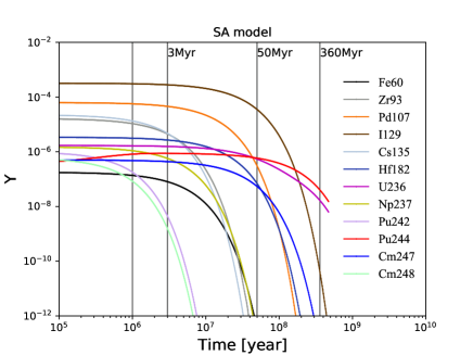
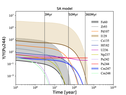
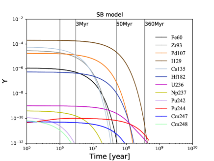
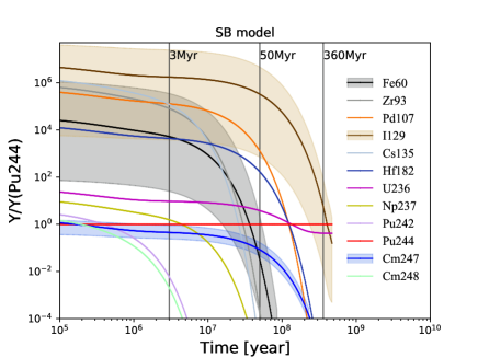
Figure 8: The time evolution of the abundances $Y$ (left) and ratios $Y$/$Y(\mbox{${}^{244}{\rm Pu}$})$ (right) of $r$-process nuclei of interest from SN model SA (top panels) and MHD SN model SB (bottom panels). The vertical lines indicate the age of the SN explosion $\sim 3$ Mya attested by discoveries of deposits of ${}^{60}{\rm Fe}$, 50 Mya comparable with the half-life of ${}^{244}{\rm Pu}$, and the age(s) of the end-Devonian extinction(s) $\sim 360$ Mya. The ratio ranges due to the nuclear variations as described in the text for ${}^{60}{\rm Fe}$, ${}^{129}{\rm I}$ and ${}^{247}{\rm Cm}$ to ${}^{244}{\rm Pu}$ are shown in shaded bands of black, brown, and blue, respectively.

The vertical lines in Fig. 8 are at 3 Myr, corresponding to the time since the event that gave rise to the well-attested deep-ocean ${}^{60}{\rm Fe}$ deposition; 50 Myr comparable with the half-life of ${}^{244}{\rm Pu}$; and 360 Myr, corresponding to the time since the end-Devonian extinction(s). The observation of ${}^{244}{\rm Pu}$ signals overlapping the ${}^{60}{\rm Fe}$ signals from 3 Mya and 7 Mya suggests that all radioisotopes with yields $Y\gtrsim Y(\mbox{${}^{244}{\rm Pu}$})$ would be interesting targets for searches in the layers containing the ${}^{60}{\rm Fe}$ signals. Depending on the model, these may include ${}^{93}{\rm Zr}$, ${}^{107}{\rm Pd}$, ${}^{129}{\rm I}$, ${}^{135}{\rm Cs}$, ${}^{182}{\rm Hf}$, ${}^{236}{\rm U}$, ${}^{237}{\rm Np}$ and ${}^{244}{\rm Pu}$, and the abundance of ${}^{247}{\rm Cm}$ may not be much smaller than that of ${}^{244}{\rm Pu}$, as seen in the right panels of Fig. 8 and in Table 5. The ratios ${}^{93}{\rm Zr}$/${}^{244}{\rm Pu}$, ${}^{107}{\rm Pd}$/${}^{244}{\rm Pu}$, ${}^{129}{\rm I}$/${}^{244}{\rm Pu}$, ${}^{135}{\rm Cs}$/${}^{244}{\rm Pu}$, and ${}^{182}{\rm Hf}$/${}^{244}{\rm Pu}$ could be particularly useful for discriminating between models, followed by ${}^{236}{\rm U}$/${}^{244}{\rm Pu}$ and ${}^{237}{\rm Np}$/${}^{244}{\rm Pu}$.

Table 5: r-Process Isotope Ratios after 3 Myr, Corresponding to the Event near the end of the Pliocene Era, together with Their Ranges $\sigma$ Found in the Different Nuclear Models Adopted (HFB Masses from Goriely et al. (2009) and $\beta$-Decay Rates from Marketin et al. (2016) for Both SN and KN Models, as well as Fission Yields from Kodama & Takahashi (1975) for KN Models), in addition to the Baseline Calculations in the $r$-Process Simulations.

Radioisotope	SN Model		KN Model
Ratio	SA	SB	KA	KB
${}^{60}{\rm Fe}$/${}^{244}{\rm Pu}$	$9.2\times 10^{-2}$	$5.3\times 10^{3}$	$2.3\times 10^{-3}$	$1.1\times 10^{-5}$
$\sigma$ (${}^{60}{\rm Fe}$/${}^{244}{\rm Pu}$)	$9.2\times 10^{-2}$ - $5.6\times 10^{2}$	25 - $3.5\times 10^{5}$	$1.4\times 10^{-3}$ - $1.3\times 10^{-2}$	$(1.1-4.0)\times 10^{-5}$
${}^{93}{\rm Zr}$/${}^{244}{\rm Pu}$	5.2	$8.2\times 10^{4}$	4.8	0.15
$\sigma$(${}^{93}{\rm Zr}$/${}^{244}{\rm Pu}$)	5.2 - $2.4\times 10^{4}$	93 - $4.3\times 10^{6}$	0.59 - 14	0.15 - 0.97
${}^{107}{\rm Pd}$/${}^{244}{\rm Pu}$	52	$1.3\times 10^{5}$	7.5	0.69
$\sigma$(${}^{107}{\rm Pd}$/${}^{244}{\rm Pu}$)	50 - $2.0\times 10^{5}$	$3.4\times 10^{2}$ - $1.7\times 10^{6}$	2.4 - 7.5	0.69 - 1.5
${}^{129}{\rm I}$/${}^{244}{\rm Pu}$	$3.2\times 10^{2}$	$1.7\times 10^{6}$	89	19
$\sigma$(${}^{129}{\rm I}$/${}^{244}{\rm Pu}$)	$2.8\times 10^{2}$ - $7.3\times 10^{5}$	$3.8\times 10^{3}$ - $2.4\times 10^{7}$	46 - 89	19 - 38
${}^{135}{\rm Cs}$/${}^{244}{\rm Pu}$	5.4	$1.2\times 10^{5}$	0.33	1.4
$\sigma$(${}^{135}{\rm Cs}$/${}^{244}{\rm Pu}$)	5.4 - $1.9\times 10^{4}$	$1.2\times 10^{2}$ - $4.1\times 10^{6}$	0.33 - 1.4	0.30 -3.9
${}^{182}{\rm Hf}$/${}^{244}{\rm Pu}$	3.1	$4.4\times 10^{3}$	0.71	0.11
$\sigma$( ${}^{182}{\rm Hf}$/${}^{244}{\rm Pu}$ )	3.1 - $2.6\times 10^{4}$	8.7 - $6.8\times 10^{4}$	0.71 - 9.0	0.11 - 2.3
${}^{232}{\rm Th}$/${}^{244}{\rm Pu}$	1.5	11	1.2	0.43
$\sigma$(${}^{232}{\rm Th}$/${}^{244}{\rm Pu}$)	0.23 - 6.0	0.31 - 16	0.36 - 1.2	0.27 - 0.63
${}^{235}{\rm U}$/${}^{244}{\rm Pu}$	1.6	7.0	1.9	0.99
$\sigma$(${}^{235}{\rm U}$/${}^{244}{\rm Pu}$ )	1.2 - 7.2	2.0 - 21	1.4 - 4.6	0.99 - 1.7
${}^{236}{\rm U}$/${}^{244}{\rm Pu}$	1.8	9.5	2.0	1.1
$\sigma$(${}^{236}{\rm U}$/${}^{244}{\rm Pu}$)	1.2 - 4.1	2.0 - 9.5	1.2 - 2.5	0.79 - 1.1
${}^{238}{\rm U}$/${}^{244}{\rm Pu}$	2.1	5.4	2.5	1.8
$\sigma$(${}^{238}{\rm U}$/${}^{244}{\rm Pu}$)	2.1 - 3.2	3.2 - 6.9	2.0 - 2.7	1.7 - 1.8
${}^{237}{\rm Np}$/${}^{244}{\rm Pu}$	0.66	1.6	0.78	0.53
$\sigma$(${}^{237}{\rm Np}$/${}^{244}{\rm Pu}$)	0.66 - 1.9	1.0 - 2.6	0.78 - 1.9	0.53 - 2.0
${}^{242}{\rm Pu}$/${}^{244}{\rm Pu}$	$5.3\times 10^{-3}$	$6.2\times 10^{-3}$	$6.0\times 10^{-3}$	$5.2\times 10^{-3}$
$\sigma$(${}^{242}{\rm Pu}$/${}^{244}{\rm Pu}$)	$(5.3-6.7)\times 10^{-3}$	$(6.2-8.8)\times 10^{-3}$	$(5.0-6.1)\times 10^{-3}$	$(5.0-5.6)\times 10^{-3}$
${}^{247}{\rm Cm}$/${}^{244}{\rm Pu}$	0.50	0.45	0.50	0.46
$\sigma$(${}^{247}{\rm Cm}$/${}^{244}{\rm Pu}$)	0.48 - 0.87	0.24 - 0.90	0.62 - 1.2	0.46 - 1.4
${}^{248}{\rm Cm}$/${}^{244}{\rm Pu}$	$1.9\times 10^{-3}$	$2.1\times 10^{-3}$	$1.6\times 10^{-3}$	$1.9\times 10^{-3}$
$\sigma$(${}^{248}{\rm Cm}$/${}^{244}{\rm Pu}$)	$(1.3-1.9)\times 10^{-3}$	$(1.0-2.1)\times 10^{-3}$	$(1.5-2.3)\times 10^{-3}$	$(1.9-2.2)\times 10^{-3}$

However, only a fraction of the reported ${}^{244}{\rm Pu}$ may have been generated by the events producing the ${}^{60}{\rm Fe}$ deposition peaks, with the remainder being due to one or more earlier astrophysical events. In this case it is natural to compare abundances on a time-scale of $\sim 50$ Myr, which is comparable with the half-life of ${}^{244}{\rm Pu}$, corresponding to the central vertical lines in the right panels of Fig. 8. On this time scale, as seen in this figure and in Table 6, the most interesting remaining isotopes are ${}^{107}{\rm Pd}$, ${}^{129}{\rm I}$, ${}^{182}{\rm Hf}$, ${}^{236}{\rm U}$, and ${}^{244}{\rm Pu}$, with the first three providing the greatest discriminating power, albeit with similar nuclear model uncertainties to those discussed above (not shown).

Table 6: r-Process Isotope Ratios after 50 Myr, comparable with the half-life of ${}^{244}{\rm Pu}$.

Radioisotope	SN Model		KN Model
Ratio	SA	SB	KA	KB
${}^{60}{\rm Fe}$/${}^{244}{\rm Pu}$	$5.9\times 10^{-7}$	$3.2\times 10^{-2}$	$1.4\times 10^{-8}$	$6.6\times 10^{-11}$
${}^{93}{\rm Zr}$/${}^{244}{\rm Pu}$	$1.5\times 10^{-7}$	$2.0\times 10^{-4}$	$1.2\times 10^{-8}$	$3.8\times 10^{-10}$
${}^{107}{\rm Pd}$/${}^{244}{\rm Pu}$	$0.53$	$1.3\times 10^{3}$	$7.6\times 10^{-2}$	$6.9\times 10^{-3}$
${}^{129}{\rm I}$/${}^{244}{\rm Pu}$	$60$	$3.3\times 10^{5}$	17	$3.5$
${}^{135}{\rm Cs}$/${}^{244}{\rm Pu}$	$2.0\times 10^{-10}$	$4.5\times 10^{-6}$	$1.2\times 10^{-11}$	$5.4\times 10^{-11}$
${}^{182}{\rm Hf}$/${}^{244}{\rm Pu}$	$0.12$	$1.7\times 10^{2}$	0.028	$4.4\times 10^{-3}$
${}^{232}{\rm Th}$/${}^{244}{\rm Pu}$	$4.6$	$28$	$4.2$	$2.1$
${}^{235}{\rm U}$/${}^{244}{\rm Pu}$	$2.9$	$11$	$3.4$	$2.0$
${}^{236}{\rm U}$/${}^{244}{\rm Pu}$	$0.93$	$3.8$	$1.0$	$0.68$
${}^{238}{\rm U}$/${}^{244}{\rm Pu}$	$3.2$	$8.1$	$3.8$	$2.6$
${}^{247}{\rm Cm}$/${}^{244}{\rm Pu}$	$9.3\times 10^{-2}$	$8.4\times 10^{-2}$	$9.2\times 10^{-2}$	$8.5\times 10^{-2}$

Finally, after 360 Myr, corresponding to the age of the end-Devonian mass extinctions, the ${}^{244}{\rm Pu}$ abundance would have decreased by an order of magnitude, relatively few radioisotopes would have survived, and only uranium isotopes, ${}^{232}{\rm Th}$, and ${}^{129}{\rm I}$ might have abundances comparable to that of ${}^{244}{\rm Pu}$, as seen in Table 7. Measurements of ${}^{129}{\rm I}$ should be able to distinguish between SN models, but not other radioisotopes.

Table 7: r-Process Isotope Ratios after 360 Myr, corresponding to the time since the end-Devonian mass extinction(s).

Radioisotope	SN Model		KN Model
Ratio	SA	SB	KA	KB
${}^{129}{\rm I}$/${}^{244}{\rm Pu}$	$4.1\times 10^{-3}$	$30$	$1.3\times 10^{-3}$	$2.3\times 10^{-4}$
${}^{232}{\rm Th}$/${}^{244}{\rm Pu}$	$85$	$4.4\times 10^{2}$	$81$	$49$
${}^{235}{\rm U}$/${}^{244}{\rm Pu}$	$30$	$1.1\times 10^{2}$	$34$	$20$
${}^{236}{\rm U}$/${}^{244}{\rm Pu}$	$0.41$	$0.42$	$0.41$	$0.41$
${}^{238}{\rm U}$/${}^{244}{\rm Pu}$	$41$	$1.0\times 10^{2}$	$48$	$33$

The results of analogous calculations for the KN models KA and KB are shown in the upper and lower panels of Fig. 9, respectively, with yields $Y$ in the left panels and the ratios $Y/Y(\mbox{${}^{244}{\rm Pu}$})$ in the right panels. As seen in this figure and in Table 5, the radioisotopes ${}^{93}{\rm Zr}$, ${}^{107}{\rm Pd}$, ${}^{129}{\rm I}$, ${}^{135}{\rm Cs}$, ${}^{182}{\rm Hf}$, ${}^{236}{\rm U}$, ${}^{237}{\rm Np}$, ${}^{244}{\rm Pu}$, and ${}^{247}{\rm Cm}$ are again the most promising potential signatures after 3 Myr or 7 Myr, with ${}^{93}{\rm Zr}$, ${}^{107}{\rm Pd}$, ${}^{129}{\rm I}$ and ${}^{182}{\rm Hf}$ offering the greatest discriminating power between KN models, and also between them and the SNS models. After 50 Myr, as seen in Table 6, the most promising radioisotopes for detection are ${}^{129}{\rm I}$ and ${}^{236}{\rm U}$. However, ${}^{236}{\rm U}$ offers little discriminating power between the different KN models, nor between the SN and KN models. After 360 Myr, as also seen in Fig. 9 and in Table 7, the best prospects for detection are again offered by ${}^{236}{\rm U}$, which does not discriminate among the KN and SN models. We do not consider ${}^{232}{\rm Th}$ and ${}^{238}{\rm U}$ to be promising search targets, in view of their long half-lives and the consequent large backgrounds from events before the formation of the solar system.

We recall that there are considerable variations in the isotope ratios calculated using the different nuclear models. In making comparisons, we have used the $\beta$-decay rates from Marketin et al. (2016), and the HFB model from Goriely et al. (2009), which assumes different nuclear masses, in addition to the baseline calculation. We note in brackets in Table 5 the ranges of isotope ratios $\sigma$ found in all the models SA, SB, KA and KB.  The ranges of predictions that come from the nuclear model variations show some overlap between the four models. We also show the ranges due to nuclear data variations in the abundance ratios of the radioisotopes ${}^{60}{\rm Fe}$, ${}^{129}{\rm I}$, and ${}^{247}{\rm Cm}$ to ${}^{244}{\rm Pu}$ as shaded bands in the right panels of Fig. 8 and Fig. 9, to illustrate the uncertainty evolution for the ratios of light elements and actinides to ${}^{244}{\rm Pu}$. The absolute abundances of ${}^{129}{\rm I}$ and lighter isotopes are relatively insensitive to the nuclear model used as shown in Fig. 7, so the uncertainties in their ratios to ${}^{244}{\rm Pu}$ are largely due to those in the ${}^{244}{\rm Pu}$ yield, and hence correlated. While the abundances of isotopes heavier than ${}^{236}{\rm U}$ are sensitive to the nuclear variations, they have similar uncertainty trends; thus their abundances relative to that of ${}^{244}{\rm Pu}$ vary over smaller uncertainty ranges, as quoted in Table 5.

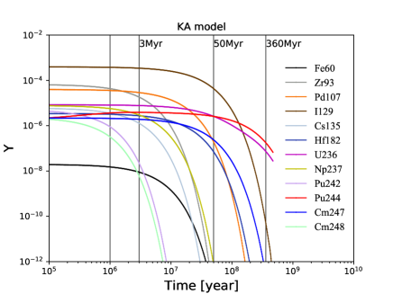
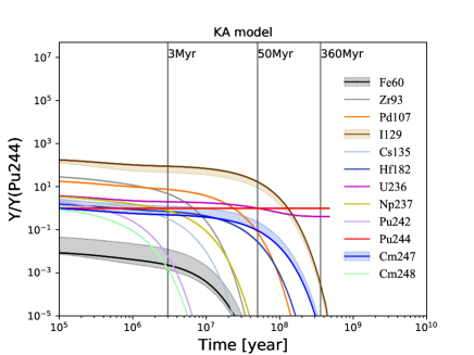
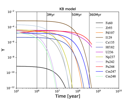
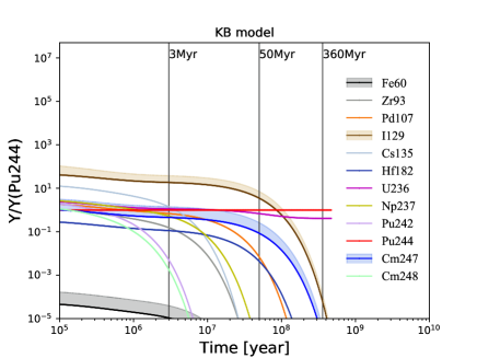
Figure 9: The time evolution of the abundances $Y$ (left) and ratios $Y$/$Y(\mbox{${}^{244}{\rm Pu}$})$ (right) of $r$-process nuclei of interest from KM models KA (top) and KB (bottom). The vertical lines correspond to the age of the SN explosion $\sim 3$ Mya attested by discoveries of deposits of ${}^{60}{\rm Fe}$, $\sim 50$ Mya comparable with the half-life of ${}^{244}{\rm Pu}$, and the time since the end-Devonian extinction(s) $\sim 360$ Mya. The ratio ranges due to the nuclear variations as described in the text for ${}^{60}{\rm Fe}$, ${}^{129}{\rm I}$ and ${}^{247}{\rm Cm}$ to ${}^{244}{\rm Pu}$ are shown in shaded bands of black, brown, and blue, respectively.

The results of our calculations of interesting abundances after 100 kyr, 3 Myr and 7 Myr (also after 50 Myr for the KN models) for the different astrophysical r-process models described in Table 3 are summarized in Fig. 10, which shows scatterplots of the isotope abundance ratios of ${}^{93}{\rm Zr}$, ${}^{107}{\rm Pd}$, ${}^{129}{\rm I}$, ${}^{135}{\rm Cs}$,${}^{182}{\rm Hf}$, and ${}^{247}{\rm Cm}$ over ${}^{244}{\rm Pu}$ versus ${}^{60}{\rm Fe}$/${}^{244}{\rm Pu}$.The asymmetric uncertainty bars reflect the ranges of microphysics uncertainties shown in Table 5 and discussed above. Note that these ratios reflect the output purely of the r-process alone. In the case of a SN there can be additional synthesis of some of these species, and if there is mixing with multiple events this would also change the ratios.

Figure 10 shows that the ratios of all these isotopes relative to ${}^{244}{\rm Pu}$ are highest in the SB SN model. However, the ordering of the abundance ratios of the other isotopes in the different models is not universal, with model SA being the lowest for ${}^{236}{\rm U}$/${}^{244}{\rm Pu}$ and ${}^{247}{\rm Cm}$, and KB being the lowest for ${}^{93}{\rm Zr}$, ${}^{107}{\rm Pd}$, ${}^{129}{\rm I}$ and ${}^{182}{\rm Hf}$/${}^{244}{\rm Pu}$. These and other differences between the model predictions offer prospects for distinguishing between the different $r$-process models by measurements in deposits up to 50 Myr old.

We emphasize that the predicted ratios in Table 3 and Fig. 10 are for r-process production only. For the KN models, this should be indicative of the typical ejected yields for these explosions. On the other hand, for the SN models there will be additional production of some species due to other processes, as summarized in Table 1. For example, ${}^{60}{\rm Fe}$ production in hydrostatic and explosive burning will far exceed that made in any SN r-process, and ${}^{93}{\rm Zr}$, ${}^{107}{\rm Pd}$, ${}^{135}{\rm Cs}$, and ${}^{182}{\rm Hf}$ could be also produced by an $s$-process in an earlier stage of stellar evolution and ejected in the SN event. Thus for these species the ratios to ${}^{244}{\rm Pu}$ in the SN models should be viewed as lower limits. Even so, they retain their discriminatory power, particularly the ${}^{60}{\rm Fe}$/${}^{244}{\rm Pu}$ ratio.

The vertical shaded band in Fig. 10 shows the the isotope ratios of ${}^{60}{\rm Fe}$/${}^{244}{\rm Pu}$ measured at 3 Myr (1.34-4.57 Myr; dark gray) and 7 Myr (4.57-9.0 Myr; gray) time periods from Wallner et al. (2021). We see that, as discussed in Section 6.1, comparing this measurement to the ${}^{60}{\rm Fe}$/${}^{244}{\rm Pu}$ ratios from our calculations excludes the KN models as the sole source of both isotopes. This is consistent with Fry et al. (2015), which excluded KNe as the source of the 3 Myr ${}^{60}{\rm Fe}$ pulse.

To lend support to our conclusions, we compare our radioisotope ratios to those from Goriely & Janka (2016) and Côté et al. (2021). Our SA model’s ${}^{247}{\rm Cm}$/${}^{244}{\rm Pu}$ ratios at 1 Myr are consistent with the SN neutrino-driven wind calculations presented in Goriely & Janka (2016). We find our SB, KA, and KB model ratios to be largely consistent with the radioisotope abundances from the data sets for the analogous simulations reported in Côté et al. (2021) at 1 Myr, i.e., our combined KN models’ radioisotope ratios are well within the uncertainty ranges of those data sets. The one notable difference is in the actinide abundances resulting from the adopted MHD SN models. The MHD SN model from Côté et al. (2021) shows more robust actinide production than our SB model, resulting in somewhat lower ratios to ${}^{244}{\rm Pu}$, while our SB model ratios are more consistent with recent simulation results from Reichert et al. (2021). Current MHD SN models exhibit conditions that only marginally reach the actinides, which results in a large astrophysical uncertainty in the ${}^{244}{\rm Pu}$ yield and a distinct contrast to the KN models.

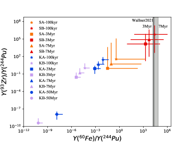
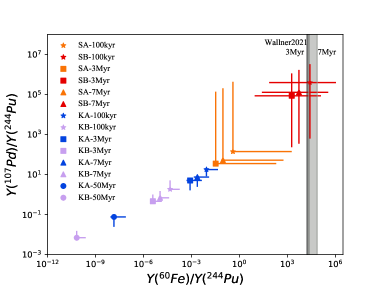
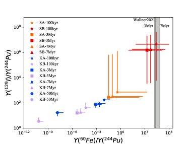
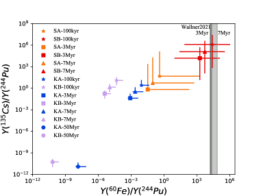
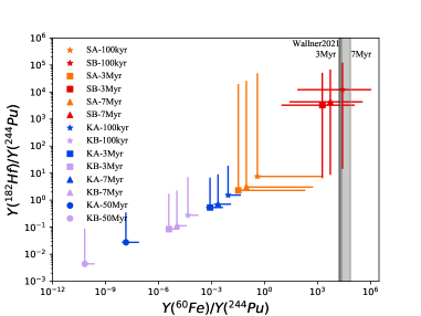
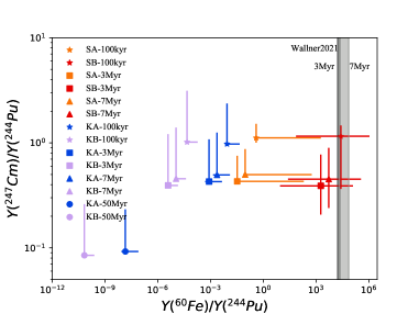
Figure 10: Scatterplots of the isotope abundance ratios of ${}^{93}{\rm Zr}$, ${}^{107}{\rm Pd}$, ${}^{129}{\rm I}$, ${}^{135}{\rm Cs}$,${}^{182}{\rm Hf}$, and ${}^{247}{\rm Cm}$/${}^{244}{\rm Pu}$ versus ${}^{60}{\rm Fe}$/${}^{244}{\rm Pu}$ after times 100 kyr, 3 Myr and 7 Myr (also 50 Myr for the KN models KA and KB), as calculated with the different astrophysical r-process models described in Table 3. The points are the isotope ratios obtained from the baseline $r$-process calculations, and the error bars denote the variations due to the different sets of nuclear models (HFB masses from Goriely et al. (2009) or $\beta$-decay rates from Marketin et al. (2016) for both SN and KN models, or fission yields from Kodama & Takahashi (1975) for KN models, in addition to the baseline nuclear data) adopted in the $r$-process. Note that the isotope ratios presented here are only from the $r$-process nucleosynthesis. For SNe, ${}^{60}{\rm Fe}$ is mainly produced in the pre-SN stage and through explosive nucleosynthesis; thus the isotope ratios of ${}^{60}{\rm Fe}$/${}^{244}{\rm Pu}$ in the plot are actually the lower limit for SN models SA and SB. The shaded bands are the measured isotope ratios of ${}^{60}{\rm Fe}$/${}^{244}{\rm Pu}$ at $\sim$3 Myr (1.34-4.57 Myr; dark gray) and $\sim$7 Myr (4.57-9.0 Myr; gray) time periods from Wallner et al. (2021).

In order to make predictions for measurements of radioisotopes like ${}^{244}{\rm Pu}$ we need, in addition to their abundances $Y_{i}(t)$ obtained from the network calculation, estimates of the total $r$-process yields or ejected masses $M_{\rm ej}$ from our SN and KN models, from which we can obtain the absolute yields for the radioisotopes $i$ at time $t$, namely $M_{i}(t)=M_{\rm ej}\times A_{i}Y_{i}(t)$. The nucleosynthetic outcome of our SA model is similar to that of the 2.2 $M_{\odot}$ neutrino-driven wind model from Wanajo (2013), where a total yield of $1.37\times 10^{-5}M_{\odot}$ is reported; estimates of the mass ejected in SN neutrino-driven winds vary from $1\times 10^{-5}M_{\odot}$ to $5\times 10^{-4}M_{\odot}$ (see, e.g., Wanajo et al., 2001; Argast et al., 2004). The yield from the MHD SN simulation we adopt for our SB model is $\sim 0.03M_{\odot}$ (Mösta et al., 2018), while a wide range of MHD SN yields are found in the literature, from $6.72\times 10^{-3}M_{\odot}$ in Winteler et al. (2012) to $\sim 0.389M_{\odot}$ in Reichert et al. (2021). For the KN models, the yield from our chosen Bovard et al. (2017) dynamical ejecta simulation is about $3.53\times 10^{-3}M_{\odot}$, which is roughly consistent with the yield in, e.g., Radice et al. (2018) of $\sim 2\times 10^{-3}M_{\odot}$. The disk wind yields from Just et al. (2015) range from $\sim 7\times 10^{-3}$ to $6.68\times 10^{-2}M_{\odot}$, similar to the range found in, e.g., Fernández et al. (2015), of $\sim 0.03$ to $0.22M_{\odot}$. For our KB model, the disk and dynamical ejecta masses are similar, giving a total yield of $7\times 10^{-3}M_{\odot}$, while for our KA model the disk wind mass is roughly four times that of the dynamical ejecta for a total yield of $1.7\times 10^{-2}M_{\odot}$. The theoretical estimates quoted above give ranges for $r$-process yields of $\sim 5\times 10^{-3}M_{\odot}-0.1M_{\odot}$, consistent with the values suggested by the observations of GW170817 (Côté et al., 2018).

Following this survey of r-process radioisotope production in SNe and KNe, we now turn to the prospects for searches in deep-ocean deposits and in the lunar regolith.

6 Models for Deep-ocean $r$-Process Radioisotopes from Stellar Explosions

We now have the tools in place to interpret the deep-ocean ${}^{244}{\rm Pu}$ (and ${}^{60}{\rm Fe}$) in light of our SN and KN models.

6.1 ${}^{244}{\rm Pu}$ Radioactivity Distance Constraints on an Event 3 Myr Ago

We first consider the possibility that the ${}^{244}{\rm Pu}$ flux coincident with the ${}^{60}{\rm Fe}$ pulse $\sim 3$ Mya is due to the same event. Thus, any ${}^{244}{\rm Pu}$ flux outside of this timespan must come from another process, such as that explored in the following section. We also assume that the radioisotope delivery is a one-step process, i.e., the terrestrial and lunar deposition of these species is a direct consequence of the propagation of the explosion ejecta.

Consider an explosion at distance $r$ and time $t$ in the past. If the explosion is isotropic, the time-integrated flux, i.e., the fluence, of radioisotope $i$ at the Sun’s interstellar location is

$${\cal F}_{i}^{\rm interstellar}=f_{i}\ \frac{M_{{\rm ej},i}/A_{i}m_{u}}{4\pi r^{2}}\ e^{-t/\tau_{i}}\,,$$ (6)

where the radioactive decay factor includes all decay in the interval $t$ between the explosion and the present time $t$, i.e., including both travel time and the duration since arrival. Here the isotope’s mass number is $A_{i}$, its mean life is $\tau_{i}$, and $m_{u}\approx m_{p}$ is the atomic mass unit. Also $M_{{\rm ej},i}$ is the yield at the time of the explosion, i.e., the total mass of isotope $i$ ejected, the total mass of isotopes ejected at explosion time is $M_{{\rm ej}}=\sum_{i}{M_{{\rm ej,i}}}$, and $f_{i}\leq 1$ is the fraction of atoms of $i$ that are incorporated into dust particles that arrive at Earth (Benitez et al., 2002; Athanassiadou & Fields, 2011; Fry et al., 2016).

After fallout onto the Earth and accumulation into natural archives such as deep-ocean sediments and crusts, the present-day surface density is (Ellis et al., 1996; Fry et al., 2015)

$$N_{i}=\frac{U_{i}{\cal F}_{i}}{4}=U_{i}f_{i}\ \frac{M_{{\rm ej},i}/A_{i}m_{u}}{16\pi r^{2}}\,\ e^{-t/\tau_{i}}\,,$$ (7)

where the factor of 4 accounts for the ratio of the Earth’s cross section to its surface area and we have included a decay factor. Here the uptake factor $U_{i}$ measures the fraction of incident atoms of $i$ that are incorporated into the sample. Fry et al. (2016) note that the fallout will not be uniform over the Earth, favoring midlatitudes at the expense of the poles and equator. Thus the effective uptake can be different at different sites for this reason alone, in addition to variations in geological conditions.

We can infer the ${}^{244}{\rm Pu}$ yield for a given explosion distance within this picture. We focus here on the time interval $\sim 3$ Mya that contains the better-measured ${}^{60}{\rm Fe}$ pulse, whose duration is at least equal to that of the nonzero ${}^{60}{\rm Fe}$ signal seen in sediments, $\Delta t=1.6\ \rm Myr$. Integrating the ${}^{244}{\rm Pu}$ flux from eq. (4) over this time, we find an interstellar ${}^{244}{\rm Pu}$ fluence ${\cal F}_{244}^{\rm interstellar}=2670\pm 560\ \rm atoms\ cm^{-2}$. Using this and the ${}^{244}{\rm Pu}$ mass yields $M_{\rm ej,244}$ calculated within the SN and KN models, we can invert eq. (6) to infer the explosion distance:

$$D_{\rm rad}(\mbox{${}^{244}{\rm Pu}$})=\sqrt{f_{\rm dust}\frac{M_{\rm ej,244}/244m_{\rm u}}{4\pi{\cal F}_{244}^{\rm interstellar}}}\ \ e^{t_{\rm exp}/2\tau_{\rm 244}}\,.$$ (8)

This “radioactivity distance” is the analog of a standard luminosity distance, with the yield playing the role of luminosity, and the fluence playing the role of flux (Ellis et al., 1996; Fry et al., 2015).

Figure 11 shows the radioactivity distance for our four r-process models, assuming that most of the ${}^{244}{\rm Pu}$ is incorporated into dust, $f_{\rm dust}^{\rm Pu}\simeq 1$. We see that the central value of the distance estimate in the MHD model SB is $\sim 100$ pc, with an uncertainty of about an order of magnitude in either direction. The forced neutrino-driven wind model SA has somewhat larger yields and thus requires larger distances, but within uncertainties the distance range overlaps with the MHD model.

These ${}^{244}{\rm Pu}$-based distances are quite consistent with the explosion distance inferred (Fields et al., 2005; Fry et al., 2015; Breitschwerdt et al., 2016) for an SN that could have generated the well-established ${}^{60}{\rm Fe}$ pulse $\sim 3$ Mya. This range, $D_{\rm rad}(\mbox{${}^{60}{\rm Fe}$})=20-150\ \rm pc$, is represented by the yellow band in Fig. 11. Within the uncertainties, this distance estimate is also compatible with the distances to the Tucana-Horologium and Scorpius-Centaurus stellar associations, which have been proposed as possible locations of the SN that generated the ${}^{60}{\rm Fe}$ pulse (Benitez et al., 2002; Breitschwerdt et al., 2012; Mamajek, 2015). Note that these results assume $f_{\rm dust}^{\rm Pu}\simeq 1$. Smaller distances would follow if a smaller value for dust efficiency is adopted; within the large yield uncertainties, these SN models remain consistent with ${}^{60}{\rm Fe}$ for dust efficiency values down to $f_{\rm dust}\sim 0.01$.

Thus we see that the ${}^{244}{\rm Pu}$ signal overlapping with the 3 Myr ${}^{60}{\rm Fe}$ pulse can be explained by an SN explosion, but only one that is r-process-enhanced. As seen in Fig. 11, such an event can give consistent distance estimates or equivalently a consistent ${}^{60}{\rm Fe}$/${}^{244}{\rm Pu}$ ratio. We also see that these distances lie between the “kill” radius $r_{\rm kill}\sim 10\ \rm pc$ and the distance at which the remnant would fade away, $r_{\rm fade}\sim 160\ \rm pc$, which provide lower and upper bounds on the distance to a nearby SN event whose radioisotope signal would be detectable. We note that the earlier ${}^{60}{\rm Fe}$ pulse at $\sim 7\ \rm Myr$ has similar but somewhat smaller fluence, and so would give a similar but somewhat smaller radioactive distance range. This too could also in principle be explained by an SN, but must again have been an r-process-enhanced event. However, such events are at best atypical of SN explosions and, as we have noted, in most modern SN models there is no actinide production at all. It is, therefore, particularly unlikely to have two such events in close succession. We will return to this point in the next section.

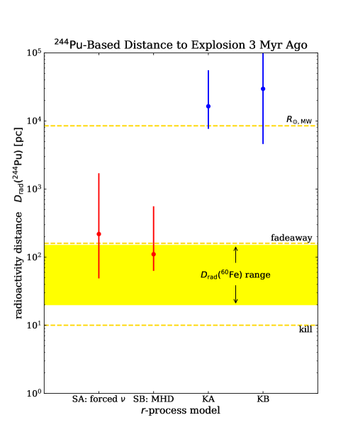
Figure 11: The estimated radioactivity distances to possible events that are candidates for having produced ${}^{244}{\rm Pu}$ 3 Mya. The distance $D_{\rm rad}\sim(f_{\rm dust}M_{\rm ej,244}/{\cal F}_{244}^{\rm interstellar})^{1/2}$ depends on the dust fraction, the model yield of ${}^{244}{\rm Pu}$, and the interstellar flux. We see that SN models lead to distances consistent with that inferred from ${}^{60}{\rm Fe}$ data, shown in the yellow band, and lie between the “kill” and “fadeaway” distances. On the other hand, KN models lead to distances far too large to allow for ${}^{244}{\rm Pu}$ transport, namely distances similar to or larger than the Sun’s distance $R_{\odot,\rm MW}$ from the Galactic center. Here we assume $f_{\rm dust}=1$; smaller values lead to smaller inferred distances.

We now turn to the possibility of a KN as the source of ${}^{244}{\rm Pu}$ 3 Mya. The yields for our KA and KB models are $\sim 6$ orders of magnitude larger than those in the SN models. As a result, Fig. 11 shows that they correspond to much larger radioactivity distances $\gg 1\ \rm kpc$. This would place the explosions implausibly far for any ejecta to reach the Earth. Indeed, the upper range of the distances extends beyond the size of our Galactic disk. Moreover, as seen in Fig. 10, the ${}^{60}{\rm Fe}$/${}^{244}{\rm Pu}$ ratio for the KN models sharply disagrees with the data. This suggests a different scenario is needed for the KN case, to which we now turn.

6.2 ${}^{244}{\rm Pu}$ Constraints on a KN Enrichment of the Local Bubble

As discussed above, the seemingly straightforward association of the ${}^{244}{\rm Pu}$ signals with the ${}^{60}{\rm Fe}$ pulses would require two consecutive rare, r-process-enhanced SN events. This coincidence seems unlikely, particularly because we know of no reason that r-process-enhanced SNe would occur in pairs or be clustered. Lacking such a reason, the two events are independently rare and thus their occurrence in close succession is exceedingly improbable. Moreover, we have seen that the ${}^{244}{\rm Pu}$ data favor a persistent flux that may extend back to as early as 25 Mya, not necessarily an impulsive signal as seen in ${}^{60}{\rm Fe}$. This leads us to consider an r-process event that occurred earlier than the ${}^{60}{\rm Fe}$ SNe, with a KN explosion being an obvious candidate. We have also seen above that a KN scenario requires that the ${}^{244}{\rm Pu}$ was not injected directly and impulsively from a single event, but instead suggests that some form of dilution occurred between the explosion and injection in the solar system.

The requirements of early r-process creation and subsequent dilution are both met naturally if a KN exploded prior to or during the early formation of the Local Bubble, enriching the entire star-forming cloud that gave rise to the bubble. Indeed, Wallner et al. (2015) have proposed such a scenario, and here we build on their analysis.

We thus envision a two-step process in which (1) the KN ejecta propagate to and mix into the proto-Local Bubble, followed by (2) the relative motion of the Earth and r-process-enriched dust leading to a flux of $r$-process radioisotopes onto Earth. Specifically, we envision the following sequence of events. (1a) More than $\sim 25$ Mya, a KN exploded, ejecting ${}^{244}{\rm Pu}$-bearing r-process material. (1b) Some of the KN ejecta collided with and was mixed into the molecular cloud giving rise to the Local Bubble. (1c) Some of the ${}^{244}{\rm Pu}$ was incorporated into dust grains. (2) The ${}^{244}{\rm Pu}$-bearing dust subsequently bombarded the Earth.

Step 1: ${}^{244}{\rm Pu}$ injection into the proto-Local Bubble. Let a KN explode at distance $r_{\rm KN}$ from the forming Local Bubble, ejecting a yield $M_{\rm ej}(\mbox{${}^{244}{\rm Pu}$})$. If the molecular cloud progenitor of the bubble has radius $R_{\rm MC}$, then the mass intercepted by the bubble and becoming dust is

$$M_{244}^{\rm LB,dust}=\frac{\pi R_{\rm MC}^{2}}{4\pi r_{\rm KN}^{2}}f_{244}M_{\rm ej}(\mbox{${}^{244}{\rm Pu}$})=\pi R_{\rm MC}^{2}\ m_{244}\ {\cal F}_{244}(r_{\rm KN})\,,$$ (9)

with $f_{244}<1$ accounting for the fraction of incident ${}^{244}{\rm Pu}$ stopped by the bubble and ultimately incorporated into grains. We see that this is just the expression in eq. (7), for the one-step interstellar KN fluence ${\cal F}_{244,KN}$ at $r_{\rm KN}$, multiplied by the cloud cross section and the atomic ${}^{244}{\rm Pu}$ mass $m_{244}$. Below we use the data, and KN rate information, to estimate the distance $r_{\rm KN}$ and evaluate its reasonableness.

Step 2: ${}^{244}{\rm Pu}$ transport to Earth. Given the ${}^{244}{\rm Pu}$ mass in eq. (9), we now estimate the ${}^{244}{\rm Pu}$ flux onto Earth. Within the bubble, the interstellar ${}^{244}{\rm Pu}$ number flux is $\Phi_{244}=n_{244}v_{\rm rel}$, with $n_{244}$ the number density and $v_{\rm rel}$ the relative velocity with respect to Earth. We expect both factors to vary with time, as ${}^{244}{\rm Pu}$-bearing dust moves in the turbulent medium constantly stirred by SNe. We do not attempt to capture these variations but only estimate average values. We then demand that these match the observed mean flux $\Phi_{244}^{\rm interstellar}$ in eq. (5), and use the results to constrain this model.

We describe the Local Bubble crudely, as a sphere of radius $R_{\rm LB}$, so that the ${}^{244}{\rm Pu}$ average number density is $n_{244}=M_{244}^{\rm LB,dust}/(4\pi A_{244}m_{u}R_{\rm LB}^{3}/3)$. Let $v_{\rm rel}$ be the speed of the Local Bubble gas relative to the Sun, , so that the interstellar ${}^{244}{\rm Pu}$ number flux is $\Phi_{244}=n_{244}v_{\rm rel}\propto M_{244}^{\rm LB,dust}/R_{\rm LB}^{3}$. Since this flux is now measured, we are in a position to evaluate the ${}^{244}{\rm Pu}$ mass needed to be injected in the Local Bubble for our model, given the measured flux $\Phi_{244}$:

$$M_{244}^{\rm LB,dust} = \frac{4\pi}{3}A_{244}m_{\rm u}R_{\rm LB}^{3}\frac{\Phi_{244}^{\rm obs}}{v_{\rm rel}}$$ (10)

$$= 6\times 10^{-11}M_{\odot}\ \left(\frac{\Phi_{244}^{\rm obs}}{1670\ \rm cm^{-2}\ Myr^{-1}}\right)\ \left(\frac{R_{\rm LB}}{50\ \rm pc}\right)^{3}\ \left(\frac{30\ \rm km/s}{v_{\rm rel}}\right)\,.$$

We use for the fiducial velocity in eq. (10) a value comparable to the Sun’s present motion with respect to the local standard of rest. This is conservative in that SN blasts and turbulent motions in the Local Bubble will in general add to the relative velocity.

We see from eq. (10) that the ${}^{244}{\rm Pu}$ inventory is far below the levels of KN yields. This implies that the explosion was not contained in the Local Bubble, but occurred outside it with only a fraction of the yield intercepted by the locally. This dilution is the main motivation for the two-step model, allowing it to avoid the unphysically large KN distances seen in the one-step picture (Fig. 11).

We note that it is likely that KN ejecta are unable to form significant amounts of dust, due to their high velocities (Takami et al., 2014; Gall et al., 2017). This is expected as a continuation of the trend in which Type Ia SNe have smaller or no dust formation compared to core-collapse explosions, which have slower ejecta speeds (Nozawa et al., 2011; Gomez et al., 2012). In light of the need for dust grains to deliver ejecta to Earth, the lack of KN dust production argues against direct, one-step deposition of ejecta from these explosions. However, in the two-step model the KN ejecta are stopped and mixed into the proto-Local Bubble material and can then be incorporated into dust grains.

We can go further and estimate the distance from the KN to the Local Bubble. This is a variant of the radioactivity distance calculation, similar to the Looney et al. (2006) calculation of the SN injection of radioisotopes into the pre-solar nebula (see, e.g., Ouellette et al., 2009). We can then solve for the KN distance, finding

$$r_{\rm KN} = \sqrt{\frac{f_{244}M_{\rm ej}(\mbox{${}^{244}{\rm Pu}$})}{4M_{244}^{\rm LB,dust}}}\ R_{\rm MC}$$ (11)

$$= 2000\ {\rm pc}\ f_{244}^{1/2}\ \left(\frac{M_{\rm ej}(\mbox{${}^{244}{\rm Pu}$})}{10^{-4}M_{\odot}}\right)^{1/2}\ \left(\frac{10^{-10}M_{\odot}}{M_{244}^{\rm LB,dust}}\right)^{1/2}\ \left(\frac{R_{\rm MC}}{3\ \rm pc}\right)\,.$$ (12)

For our fiducial quantities and $f_{244}<1$, we have $r_{\rm KN}\lesssim 2$ kpc. This places the KN explosion at a distance that is more consistent with the expectation that KNe are rarer and further between than SNe.  We note that a KN is likely to be so distant that its ejecta blast would be weak when arriving in the solar neighborhood, and hence unlikely to destroy the local molecular cloud.

Estimates of KN and neutron star merger rates place consistency checks on our distance calculations (Hartmann et al., 2002; Scalo & Wheeler, 2002). The average rate for a KN within distance $r_{\rm KN}$ is $\Gamma(r_{\rm KN})\approx\pi r_{\rm KN}^{2}\ Q_{\rm local}$ where $Q_{\rm local}=dN_{\rm KN}/dA\,dt$ is the KN rate per unit area of the Galactic disk at the solar location; we assume $r_{\rm KN}>h$, the scale height of KN progenitors, so that the problem is reduced to two dimensions. Using the usual approximation of an exponential disk with scale radius $R_{0}=2.9$ kpc (see, e.g., Girardi et al., 2005; Murphey et al., 2020), we have $Q(R)={\cal R}_{\rm KN}e^{-R/R_{0}}/2\pi R_{0}^{2}$, where the total Galactic KN rate sets the normalization via the surface integral ${\cal R}_{\rm KN}=2\pi\int Q(R)\ R\ dR$. We estimate the Galactic KN rate assuming the ratio to the Galactic core-collapse SN rate ${\cal R}_{\rm CC}$ is the same as the ratio of the local cosmic rate densities: ${\cal R}_{\rm KN}/{\cal R}_{\rm CC}=\dot{\rho}_{\rm KN}/\dot{\rho}_{\rm CC}$. Using ${\cal R}_{\rm CC}\approx 0.032\ \rm yr^{-1}$ (Adams et al., 2013), $\dot{\rho}_{\rm CC}=1.1\times 10^{-4}\ {\rm Mpc}^{-3}\,\rm yr^{-1}$ (Lien & Fields, 2009), and a binary neutron star merger rate as a measure of the underlying r-process source rate $\dot{\rho}_{\rm BNS}\gtrsim\dot{\rho}_{\rm KN}\sim 1500\ {\rm Mpc}^{-3}\,{\rm yr}^{-1}$ (consistent with estimates from Matteucci et al., 2014; Wehmeyer et al., 2015; Chruslinska et al., 2018; Côté et al., 2018; Della Valle et al., 2018; Jin et al., 2018; Andreoni et al., 2020, 2021), we find $R_{\rm KN}\sim 1.4\times 10^{-2}{\cal R}_{\rm SN}\sim 440\ \rm Myr^{-1}$. Finally

$$\Gamma_{\rm KN}\sim 1.3\ {\rm events\ Myr^{-1}}\ \left(\frac{r_{\rm KN}}{1\ \rm kpc}\right)^{2}$$ (13)

at the solar distance from the center of the galaxy, i.e., $r_{\rm KN}=R_{\odot}=8.7$ kpc. We see that the typical KN recurrence time is $\Gamma_{\rm KN}^{-1}\sim 0.8\ \rm Myr\ (1\,\rm kpc/r_{\rm KN})^{2}$. Thus KN explosion times of $t_{\rm KN}=(10,50)\ \rm Myr$ correspond to mean distances of $r_{\rm KN}=(280,120)$ pc. Our two-step ${}^{244}{\rm Pu}$-based radioactivity distances lie comfortably within this range, demonstrating overall consistency.

Two other issues constrain the timing of the KN explosion and subsequent r-process rain. One is the timescale for the Local Bubble to assemble and form stars; this timescale plus massive-star lifetimes sets an upper limit to the KN injection time. The Fuchs et al. (2006) fit to massive-star lifetimes gives 23 (18) Myr for masses $\geq 8(10)M_{\odot}$ at the threshold of core collapse, and the lifespans are nearly linearly dependent on the inverse of the mass. Estimates of the lifetimes of molecular clouds span a significant range from local solar neighborhood values of a few Myr (Hartmann et al., 2001) to $\sim 30\ \rm Myr$ (Murray, 2011). For the Local Bubble itself, based on lifetimes of extant stars and pulsars, as well as on expansion dynamics, Breitschwerdt et al. (2009, 2016) estimate an age $\sim 15\ \rm Myr$ and $\sim 17$ SNe, which is consistent with the Maiz-Apellaniz (2001) argument for $\sim 20$ SNe during the last 10-12 Myr. On the other hand, Abt (2011) argues that some portions of the bubble could be as old as $\sim 50\ \rm Myr$, whereas Smith & Cox (2001) consider models with ages $\lesssim 10\ \rm Myr$ and three SNe. We therefore consider a range of KN injection timescales of $(10,20,50)$ Myr, as noted in eq. (2).

Finally, the r-process bombardment on Earth can begin only when the Sun enters the Local Bubble. This time is uncertain and depends on the evolving bubble morphology, but also sets an upper limit on the injection time.

We observe that this two-step process incurs larger uncertainties overall than the one-step SN mechanism. One of them is the timing of the KN: the further in the past, the greater the losses of shorter-lived species. If the ${}^{244}{\rm Pu}$ event in the 12.5–25 Mya crust layer is real, it sets a lower limit on this time. The longest-lived $r$-process radioisotopes of interest, apart from ${}^{244}{\rm Pu}$, are ${}^{129}{\rm I}$, ${}^{182}{\rm Hf}$, and ${}^{247}{\rm Cm}$. These live long enough for their production in a KN to be potentially observable in this layer; also the secular equilibrium abundance of ${}^{236}{\rm U}$ potentially provides a check on anthropogenic sources of actinides.

6.3 Predicting r-Process Radioisotope Signatures in Terrestrial Archives

The previous two subsections show that it is possible to construct both SN and KN scenarios for some or all of the ${}^{244}{\rm Pu}$ signal. We conclude that the ${}^{244}{\rm Pu}$ flux in eqs. (4) and (5) could have an astrophysical origin, and use these to normalize our subsequent predictions for possible live isotope searches using AMS techniques. In this section we compute terrestrial signals for additional r-process radioisotopes, with a particular focus on Fe-Mn crusts. Our strategy is to pursue the consequences of the ${}^{244}{\rm Pu}$ detection, using it to infer the abundances of other r-process radioisotopes predicted by our SN and KN models.

The available natural terrestrial archives that accumulate gradually over the longest periods of time, and thereby give the most complete dating information, are deep-ocean crusts and sediments. In the natural archives of interest, radioisotope abundances are usually presented as an isotope fraction $(N_{i}/N_{j})_{\rm obs}$, the ratio of a radioisotope $i$ to a stable isotope or element $j$. Here we derive predictions for the ratio $N_{i}^{\rm astro}/N_{j}^{\rm bg}$, i.e., the astrophysical signal relative to a stable “background” isotope.

The astrophysical signal can be expressed as the incident interstellar number flux $\Phi_{i}^{\rm interstellar}=dN_{i}/dAdt$, usually given without decay losses included. The measurable flux onto a terrestrial sample is

$$\Phi_{i}^{\rm sample}=\frac{f_{i}U_{i}}{4}\Phi_{i}^{\rm interstellar}e^{-t/\tau_{i}}\,,$$ (14)

where the factor of 4 accounts for the ratio of the Earth’s cross section to its surface area, $f_{i}$ is the fraction of $i$ in dust arriving at Earth, and $U_{i}$ accounts for uptake into the sample. We have also accounted for radioactive decay. If the flux is measured for a time interval $\Delta t$, the corresponding surface density in the sample is $N_{i}^{\rm astro}=\Phi_{i}^{\rm sample}\,\Delta t$.

During this time interval, the sample accumulates a surface mass density $\rho\ \dot{h}\ \Delta t$, where $\rho$ is the total density, and $\dot{h}=dh/dt$ is the rate of growth of the thickness. Let the background species $j$ have mass fraction $X_{j}=\rho_{j}/\rho$ in the sample, and mass number $A_{j}$. Then the background atoms $j$ have surface density $N_{j}=X_{j}\rho\,\dot{h}\ \Delta t/A_{j}m_{u}$, with $m_{u}=1/N_{\rm Avo}$ the atomic mass unit. Thus

$$\frac{N_{i}^{\rm astro}}{N_{j}^{\rm bg}}=U_{i}f_{i}\frac{\Phi_{i}^{\rm interstellar}}{4X_{j}\rho\,\dot{h}/A_{j}m_{u}}e^{-t/\tau_{i}}$$ (15)

is the desired isotopic ratio.

We anchor our predictions to the detections of ${}^{244}{\rm Pu}$ discussed above. In this case we have

$$\frac{N_{i}^{\rm astro}}{N_{j}^{\rm bg}}=U_{i}\ \frac{f_{i}}{f_{\rm Pu}}\ \left(\frac{{\cal N}_{i}}{{\cal N}_{244}}\right)_{\rm astro}\ \frac{\Phi_{244,\rm astro}^{\rm interstellar}}{4X_{j}\rho\,\dot{h}/A_{j}m_{u}}e^{-t/\tau_{i}}\,,$$ (16)

where we use the fact that the interstellar flux of a species is proportional to its (number) yield, $\Phi_{i}^{\rm interstellar}\propto{\cal N}_{i}$. Using values typical for crusts, we have

$$\frac{N_{i}^{\rm astro}}{N_{j}^{\rm bg}} = 2\times 10^{-13}\ U_{i}\ \frac{f_{i}}{f_{\rm Pu}}\ \left(\frac{{\cal N}_{i}}{{\cal N}_{244}}\right)_{\rm astro}e^{-t/\tau_{i}}$$ (18)

$$\times\left(\frac{\Phi_{244}^{\rm interstellar}}{1670\ \rm cm^{-2}\,Myr^{-1}}\right)\ \left(\frac{1\ \rm ppm}{X_{j}}\right)\ \left(\frac{A_{j}}{150}\right)\ \left(\frac{2\,\rm g/cm^{3}}{\rho}\right)\ \left(\frac{3\,\rm mm/Myr}{\dot{h}}\right)\,.$$

Note that the signal is inversely proportional to both the growth rate and the background abundance in the sample: $N_{i}^{\rm astro}/N_{j}^{\rm bg}\propto(X_{j}\dot{h})^{-1}$. This favors samples with low growth rates and hence Fe-Mn crusts. It also favors elements that are rare in crusts (so long as the uptake is not too small).

Table 8: Predicted Interstellar Fluences for r-Process Radioisotopes based on ${}^{244}{\rm Pu}$

	${\cal F}({\rm 3\,Myr)}$				${\cal F}({\rm 10\,\rm Myr})$		${\cal F}({\rm 20\,\rm Myr})$		${\cal F}({\rm 50\,\rm Myr})$
Isotope	SA	SB	KA	KB	KA	KB	KA	KB	KA	KB
${}^{93}{\rm Zr}$	5.1(3)	8.0(7)	4.7(3)	1.5(2)	2.3(3)	7.5(1)	7.1(1)	2.3(0)	5.8(-4)	1.9(-5)
${}^{107}{\rm Pd}$	5.1(4)	1.3(8)	7.4(3)	6.7(2)	3.7(4)	3.4(3)	2.8(4)	2.5(3)	3.7(3)	3.4(2)
${}^{129}{\rm I}$	3.1(5)	1.7(9)	8.7(4)	1.8(4)	6.8(5)	1.4(5)	9.6(5)	2.0(5)	8.3(5)	1.7(5)
${}^{135}{\rm Cs}$	5.3(3)	1.2(8)	3.2(2)	1.4(3)	8.5(1)	3.7(2)	1.1(0)	4.7(0)	6.0(-7)	2.7(-6)
${}^{182}{\rm Hf}$	3.0(3)	4.3(6)	7.0(2)	1.1(2)	4.3(3)	6.7(2)	4.3(3)	6.8(2)	1.4(3)	2.1(2)
${}^{236}{\rm U}$	1.8(3)	9.3(3)	2.0(3)	1.1(3)	1.7(4)	1.0(4)	3.0(4)	1.8(4)	4.9(4)	3.4(5)
${}^{237}{\rm Np}$	6.4(2)	1.5(3)	7.6(2)	5.2(3)	8.1(2)	5.5(2)	7.2(1)	4.9(1)	1.5(-2)	1.0(-2)
${}^{247}{\rm Cm}$	4.9(2)	4.4(2)	4.9(2)	4.5(2)	3.8(3)	3.5(3)	5.3(3)	4.9(3)	4.5(3)	4.2(3)

Notes. The interstellar fluences ${\cal F}^{\rm interstellar}$ are normalized relative to the fluence of ${}^{244}{\rm Pu}$, and are expressed in units of $[\rm atoms\ cm^{-2}]$, using the notation $A(B)\equiv A\times 10^{B}$. All results are for the present day, and include the effects of decay. The signal at 3 Mya assumes a flux duration of 1 Myr, and the others assume a constant flux after the event.

Table 9: Predictions for r-Process Radioisotopes in Fe-Mn Crusts based on ${}^{244}{\rm Pu}$ after 3 Myr

	Concentration [atoms $g^{-1}$]				Ratio	Measurement	Crust Elemental	Predicted Signal Ratio
Isotope	SA	SB	KA	KB	$N_{i}^{\rm astro}/N_{j}^{\rm bg}$	Limit	Abundance $X_{j}$	SA	SB	KA	KB
${}^{93}{\rm Zr}$	6.5(2)	1.0(7)	5.9(2)	1.9(1)	${}^{93}{\rm Zr}$/${}^{92}{\rm Zr}$	$2\times 10^{-11}$	$6.5\times 10^{-4}$	8.9(-16)	1.4(-11)	8.2(-16)	2.7(-17)
${}^{107}{\rm Pd}$	6.5(3)	1.6(7)	9.4(2)	8.6(1)	${}^{107}{\rm Pd}$/${}^{106}{\rm Pd}$	$10^{-8}$	$1.7\times 10^{-9}$	2.5(-9)	6.1(-6)	3.6(-10)	3.3(-11)
${}^{129}{\rm I}$	4.0(4)	2.2(8)	1.1(4)	2.3(3)	${}^{129}{\rm I}$/${}^{127}{\rm I}$	$10^{-14}$	$5\times 10^{-6}$	1.7(-11)	9.2(-8)	4.7(-12)	9.8(-13)
${}^{135}{\rm Cs}$	6.8(2)	1.5(7)	4.2(1)	1.8(2)	${}^{135}{\rm Cs}$/${}^{133}{\rm Cs}$	$9\times 10^{-12}$	$1.5\times 10^{-6}$	1.0(-13)	2.2(-9)	6.1(-15)	2.6(-14)
${}^{182}{\rm Hf}$	3.8(2)	5.5(5)	8.9(1)	1.4(1)	${}^{182}{\rm Hf}$/${}^{180}{\rm Hf}$	$10^{-11}$	$8\times 10^{-6}$	4.5(-14)	6.4(-11)	1.0(-14)	1.7(-15)
${}^{236}{\rm U}$	2.2(2)	1.2(3)	2.5(2)	1.4(2)	${}^{236}{\rm U}$/${}^{238}{\rm U}$	$10^{-13}$	$10^{-5}$	8.9(-15)	4.7(-14)	1.0(-14)	5.7(-15)
${}^{237}{\rm Np}$	8.2(1)	2.0(2)	9.7(1)	6.6(1)	${}^{237}{\rm Np}$/${}^{238}{\rm U}$	$5\times 10^{-11}$	$10^{-5}$	3.3(-15)	7.8(-15)	3.9(-15)	2.6(-15)
${}^{247}{\rm Cm}$	6.2(1)	5.6(1)	6.2(1)	5.7(1)	${}^{247}{\rm Cm}$/${}^{238}{\rm U}$	-	$10^{-5}$	2.5(-15)	2.3(-15)	2.5(-15)	2.3(-15)

Notes. The values are expressed as $A(B)\equiv A\times 10^{B}$. The crust abundances are taken from Hein et al. (2000), and we assume $\Phi^{\rm interstellar}(\mbox{${}^{244}{\rm Pu}$})$ fluxes in eqs. (4) and (5). The uptake is assumed to be $U=0.10$ in all cases. The isotopic concentration $n_{i}^{\rm astro}/\rho$ is the number of atoms of isotope $i$ per gram of crust. The crust elemental abundances $X_{j}$ are mass fractions; for ${}^{237}{\rm Np}$ and ${}^{247}{\rm Cm}$, the uranium abundance is given. The measurement limits are the AMS sensitivities for ${}^{93}{\rm Zr}$ (Hain et al., 2018; Martschini et al., 2019; Pavetich et al., 2019), ${}^{107}{\rm Pd}$ (Korschinek et al., 1994), ${}^{129}{\rm I}$ (Vockenhuber et al., 2015), ${}^{135}{\rm Cs}$ (Yin et al., 2015) and ${}^{182}{\rm Hf}$ (Vockenhuber et al., 2004); see discussion in §6.4.

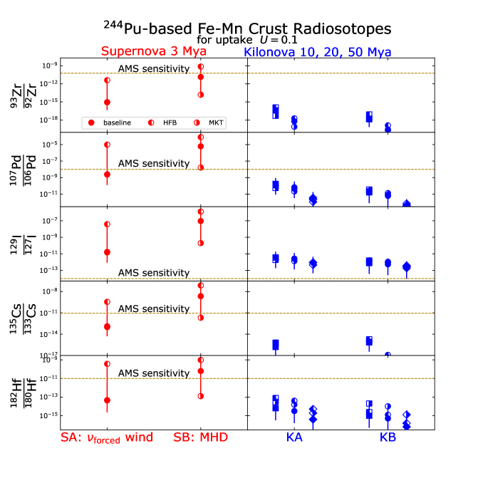
Figure 12: Radioisotope predictions normalized to the Wallner et al. (2015) ${}^{244}{\rm Pu}$ flux from Eqs. (4) and (5). The predictions are normalized to a 10% uptake, and assume dust efficiency equal to that of Pu; for other values multiply by $U_{i}f_{i}/f_{\rm Pu}$. The uncertainties are only those due to the ${}^{244}{\rm Pu}$ flux, and the measurement limits are those listed in Table 9. The predictions are from (left panels) the SN r-process models after 3 Myr and (right panels) the KN r-process models after 10, 20, and 50 Myr. The results from our baseline calculations are shown as full symbols, and the half-filled symbols are results from HFB and MKT calculations. A minor change to the figure should be made for ${}^{93}{\rm Zr}$/${}^{92}{\rm Zr}$ from $6\times 10^{-11}$ to a new value of $2\times 10^{-11}$ in light of a new citation that has been added to the text.

Tables 5-7 give the number ratios for various isotopes of interest $({\cal N}_{i}/{\cal N}_{244})_{\rm astro}e^{-t/\tau_{i}}$, where we incorporate the decay factors corresponding to the different time scales of interest. For the lighter species with stable isotopes, the candidates of particular interest are those with high ratios to ${}^{244}{\rm Pu}$.

Table 8 shows the time-integrated interstellar flux or fluence, as defined in eq. (6), for selected r-process radioisotopes in specific scenarios. The values are for the present day, and include the effects of decay. For the 3 Mya signal associated with an SN, the duration is 1 Myr. For the KN signal at 10 Myr, the duration is assumed to be 10 Myr. The fluences are the most direct results from the astrophysical calculations, but connecting them to geological and lunar measurements requires one to specify the abundances in particular samples.

Table 9 shows our predictions for selected radioisotope ratios following deposition in Fe-Mn crusts 3 Mya, normalized to a 10% uptake and $f_{i}/f_{\rm Pu}=1$. These results also appear in Fig. 12, where use the ${}^{244}{\rm Pu}$ flux inferred from sediments $0.5-2.2\,\rm Myr$ old (Wallner et al., 2015) for normalization. In general we see that the SN predictions are as large as, and sometimes much larger than, those of the KN models. This reflects the difficulty of making actinides in SN models, which means that lower-mass species are more abundant relative to the ${}^{244}{\rm Pu}$ isotope that anchors our results. Variations between the KN model predictions are generally within a factor of 10. In contrast, the SN predictions can span several orders of magnitude, with the SB model generally leading to larger low-mass abundances due to its particularly low ${}^{244}{\rm Pu}$ output. Also shown in Table 9 and Fig. 12 are the prospective AMS sensitivities for ${}^{93}{\rm Zr}$ (Hain et al., 2018; Martschini et al., 2019; Pavetich et al., 2019), ${}^{107}{\rm Pd}$ (Korschinek et al., 1994), ${}^{129}{\rm I}$ (Vockenhuber et al., 2015), ${}^{135}{\rm Cs}$ (Yin et al., 2015), and ${}^{182}{\rm Hf}$ (Vockenhuber et al., 2004). We see that, whereas predictions for the ${}^{93}{\rm Zr}$ signal generally lie below the AMS sensitivity, those for ${}^{107}{\rm Pd}$, ${}^{135}{\rm Cs}$, and possibly ${}^{182}{\rm Hf}$ in model SB lie above the AMS sensitivity, and the predictions for the ${}^{129}{\rm I}$ signal lie above the AMS sensitivity in both SN scenarios and possibly also in the KN scenarios.

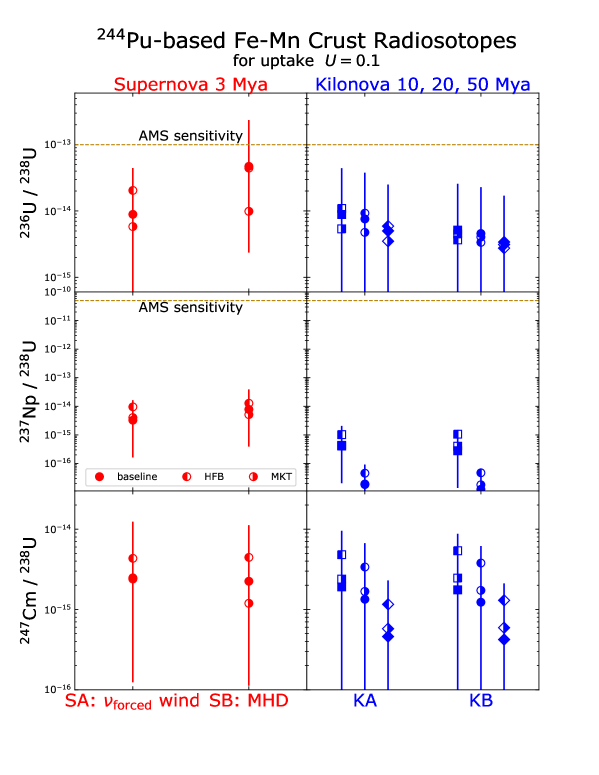
Figure 13: Predicted abundances of the actinides ${}^{236}{\rm U}$, ${}^{237}{\rm Np}$, and ${}^{247}{\rm Cm}$ in Fe-Mn crusts, shown for the same SN and KN models as in Fig. 12. We use ${}^{238}{\rm U}$ as the reference standard for all three species. The results from our baseline calculations are shown as full symbols, and the half-filled symbols are results from HFB and MKT calculations.

Figure 13 shows the Fe-Mn crust abundances for the actinides ${}^{236}{\rm U}$, ${}^{237}{\rm Np}$, and ${}^{247}{\rm Cm}$, for the same models as in Fig. 12. These are all elements with no stable isotopes, so we use ${}^{238}{\rm U}$ as a reference standard for the ratios presented; we note that ${}^{238}{\rm U}$ is also the source of ${}^{236}{\rm U}$ background. We recall that natural uranium will far overwhelm any astrophysical contribution. For this reason, the ${}^{236}{\rm U}$ signal may be masked by other production mechanisms. For ${}^{237}{\rm Np}$, suppression of the ${}^{238}{\rm U}$ signal may be necessary before a signal can be seen. We thus conclude that ${}^{236}{\rm U}$ and ${}^{237}{\rm Np}$ detections likely await improvements in measurement techniques. For ${}^{247}{\rm Cm}$, uranium is not anticipated to be a limitation, but detection will require establishing a pure curium reference spike. We urge further study of the experimental possibilities for all of these species.

To summarize, we have found that the ${}^{244}{\rm Pu}$ evidence implies that the geological record should contain other r-process radioisotope signals. The abundances are in some cases within or close to the reach of existing AMS techniques, whereas improvements in the AMS sensitivity to key species are necessary in other cases.

We emphasize that the experimental program for these new species, as well as additional ${}^{60}{\rm Fe}$ and ${}^{244}{\rm Pu}$ searches, should have two related but distinct goals: sensitivity and time resolution.

• Sensitivity. High sensitivity, i.e., the ability to detect small extraterrestrial radioisotope abundances, obviously is critical. It allows for detection of additional species and more accurate abundances, both of which sharpen the probes of the potential nucleosynthesis sites.

• Time resolution. Time resolution offers another powerful means of distinguishing between models. A better determination of the ${}^{244}{\rm Pu}$ time history can clarify whether it is exclusively coincident with the two ${}^{60}{\rm Fe}$ pulses, suggesting a common SN origin, or it appears at other epochs, suggesting a distinct origin likely in a KN. The time behavior of additional radioisotopes can then be compared with that of ${}^{60}{\rm Fe}$ and ${}^{244}{\rm Pu}$, which can further distinguish between these scenarios and potentially distinguish between SN and KN models.

These goals are in some tension, as finer time resolution implies smaller samples per time bin, reducing the available signal at a fixed sensitivity. As with the development of the ${}^{60}{\rm Fe}$ measurements, a sensible strategy may be to first strive for the detection of new species, then follow up with better time resolution.

We now turn to considerations of sample collection for each of the radioisotopes of interest.

6.4 Terrestrial Searches

In order to detect and preserve these signals, we emphasize that samples must be collected from well-chosen sites and suitable media, in the sense that the samples should have maintained a detectable abundance of the SN debris from the initial deposit to the present and that the samples should be accessible for collection and delivery to the laboratory. We consider these issues for the Earth in this section, and for the Moon in the next section.

Marine samples are the primary focus of interest as natural terrestrial archives, since continental material is subject to erosion, and radioisotope studies in ice cores do not extend so far into the past.  In general, deep-ocean deposits are essentially undisturbed, with very little disturbance from creatures at the ocean floor (bioturbation) to blur the time structure, and are largely free of anthropogenic contamination from nuclear debris, as well as backgrounds from cosmic-ray spallation in the atmosphere. Debris at the sea floor accumulates in sediments that stretch back beyond the $\sim 10$ Myr that has been studied so far, rendering it suitable for exploring possible astrophysical triggers of mass extinctions that occurred $\gtrsim 10^{8}$ ya ago in addition to the well-attested ${}^{60}{\rm Fe}$ signal, evidence for ${}^{53}{\rm Mn}$ from $\sim 3$ Mya, and reports of ${}^{244}{\rm Pu}$ deposition over the past 25 Myr. Ultimately, deep-ocean sediments may harden to make sedimentary rock in geological strata reaching back to much longer timescales. In this section and Table 10 we highlight some of the key considerations from chemical oceanography that determine which astrophysical radioisotopes may have geologically favorable conditions for detection. We make heavy use in the following discussion of Broecker et al. (1982), Nozaki (2001), and the Geotraces database  and private communications with Craig Lundstrom and Tom Johnson.

In considering the prospects for detecting marine deposits of radionuclides, one must consider the sedimentation rates of the radionuclides of interest, focusing on those with a short residence time and discarding those that remain dissolved in seawater. Table 10 lists the elements discussed earlier in this paper, together with their mean oceanic concentrations and the characteristics of their distributions, which provide the basis for our discussion of the possibilities of detecting their radioisotopes in view of the SN and KN model calculations above.

Table 10: Estimated mean oceanic concentrations of selected elements, adapted from Nozaki (2001)

Element	Mean oceanic	Type of	Leaves Solution
	mass fraction ($\times 10^{-12}$)	Distribution	Rapidly
Mn	20	s	yes
Fe	30	s + n	yes
Zr	15	s + n	yes
Pd	0.06	n	yes
I (IO${}^{-}_{3}$)	$5.8\times 10^{4}$	c	no
I (I-)	4.4	r + s	yes
Cs	310	c	no
Hf	0.07	s + n	yes
U	$3.2\times 10^{3}$	c	no
Np	$\sim 10^{-5}$	c	no
Pu	-	r + s	yes
Cm	-	s?	?

Notes. In this Table c denotes an element whose distribution is conservative, in the sense that it follows the salinity of the ocean water, n denotes a distribution that increases with depth, like that of typical nutrients in the water, s denotes an element that attaches to particulate matter and may be concentrated (“scavenged”) at the water/sediment interface, and r denotes an element whose distribution is controlled by reduction and oxidation reactions (“redox-controlled”) and may be formed in oceanic basins that are depleted in oxygen (“anoxic”) (Nozaki, 2001). ${}^{237}{\rm Np}$ results are from Lindahl et al. (2005). We note also that there may be other geochemical and biological processes that affect the rates of uptake of different radionuclides in various materials. For example, “magnetotactic” bacteria that orientate themselves along magnetic fields

secrete iron and therefore concentrate ${}^{60}{\rm Fe}$, as discussed in Ludwig et al. (2016), and certain sorts of organic matter may absorb plutonium effectively (J. Marshall, private communication, 2021), specifically in anoxic environments. Schneider & Livingston (1984) measured anthropogenic ${}^{242}{\rm Cm}$ and ${}^{244}{\rm Cm}$ in Scottish coastal sediments, and summarized data indicating that ${}^{244}{\rm Cm}$ has also been detected in fish and seaweed but not in seawater; we also note that curium adheres very tightly to soil particles.

$\bullet$ Among the elements that may be produced by the $r$-process and are identified in the previous section as being of interest, we note that zirconium sinks in the ocean, attaches to solid particles, and may be scavenged at the water/sediment interface, similarly to iron. The half-life of ${}^{93}{\rm Zr}$ ($1.53\times 10^{6}$ yr) is somewhat less than those of the isotopes ${}^{60}{\rm Fe}$ and ${}^{53}{\rm Mn}$ that have been reported in layers $\sim 2.5\times 10^{6}$ yr old. Figs. 8 and 9 and Table 5 indicate that its $r$-process production rate, which is quite model-dependent, may be orders of magnitude higher than that of ${}^{60}{\rm Fe}$, or considerably lower. However, Table 9 and Fig. 12 indicate that the ${}^{93}{\rm Zr}$ signal in 3 Myr old samples may lie below the estimated AMS sensitivity.

$\bullet$ Palladium has a distribution that increases with depth, but is not expected to bind to particles or be concentrated at the water/sediment interface. It has been detected in Fe-Mn crusts, but with low abundances (see Table 9), which is advantageous for our purposes. These low abundances imply that, as seen in Table 9 and Fig. 12, the relative abundances of ${}^{107}{\rm Pd}$ predicted in some $r$-process models may be within reach of the AMS technique if a suitable 3 Myr old sample can be found.

$\bullet$ Most iodine is in the form of the IO${}^{-}_{3}$ ion, which is distributed conservatively, but a small fraction is in the form of the I^- ion, which may be scavenged, preferentially in anoxic basins such as the Black Sea. Fitoussi & Raisbeck (2007) attempted to measure ${}^{129}{\rm I}$ in a relatively recent but pre-anthropogenic sediment, and found that care is needed to avoid anthropogenic contamination. Ji et al. (2015a) have presented the first AMS measurements of ${}^{129}{\rm I}$ in Fe-Mn crusts. These data already reveal the power of ${}^{129}{\rm I}$ to probe near-Earth explosions, particularly the possible KN enrichment of the Local Bubble, and the corresponding constraints are discussed in detail in the following Section 6.5.

$\bullet$ Cesium dissolves in water and has a conservative oceanic distribution, so ${}^{135}{\rm Cs}$ offers poor prospects for deep-ocean detection. Moreover, as seen in Table 9 and Fig. 12, most of the models studied indicate that the fraction of ${}^{135}{\rm Cs}$ may lie below the AMS sensitivity.

$\bullet$ Hafnium is an interesting target, particularly if production occurred more than 3 Mya, thanks to the ${}^{182}{\rm Hf}$ half-life of 8.9 Myr. Most of our $r$-process models produce less ${}^{182}{\rm Hf}$ than ${}^{93}{\rm Zr}$, while the oceanic distribution of hafnium is similar to that of zirconium. In a sediment, Vockenhuber et al. (2004) have established the upper limit $\mbox{${}^{182}{\rm Hf}$}/\mbox{${}^{180}{\rm Hf}$}<10^{-6}$ using a 45 g sample, and quoted a total hafnium elemental abundance by dry weight of 8 ppm. Combining these numbers, we find an upper limit on the fraction by weight of ${}^{182}{\rm Hf}$ of $8\times 10^{-12}$. Martschini et al. (2020) showed that these limits could in principle be improved dramatically using a laser technique to remove stable isobars. They found $\mbox{${}^{182}{\rm Hf}$}/\mbox{${}^{180}{\rm Hf}$}=(3.4\pm 2.1)\times 10^{-14}$, on the basis of which they estimated a sensitivity of $(\mbox{${}^{182}{\rm Hf}$}/\mbox{${}^{180}{\rm Hf}$})_{\rm min}\approx 6\times 10^{-14}$. This would correspond to a mass fraction of $\sim 4\times 10^{-18}$, which could be achieved if the stable tungsten isobar ${}^{182}{\rm W}$ is absent or can be removed.

For comparison, Wallner et al. (2021) estimated a range of $(0.1-100)\times 10^{-22}$ ${}^{244}{\rm Pu}$ atoms per atom in the crust samples. It is important to note that one major improvement for these measurements was the use of the 1 MV accelerator Vega at Australia’s Nuclear Science and Technology Organisation, which provided an improved ${}^{244}{\rm Pu}$ detection efficiency from $1\times 10^{-4}$ (Wallner et al., 2015) to $1.5\%$. These measurements correspond to a sensitivity to the fraction by weight of $\sim 10^{-22}$. In Table 5 we see ratios $\mbox{${}^{182}{\rm Hf}$}/\mbox{${}^{244}{\rm Pu}$}<8.7\times 10^{4}$ (reached in model SB), suggesting that the model sensitivity of the ${}^{244}{\rm Pu}$ detection by Wallner et al. (2021) is better than that of the ${}^{182}{\rm Hf}$ search by Vockenhuber et al. (2004), though a more sensitive ${}^{182}{\rm Hf}$ search may have interesting prospects. Vockenhuber et al. (2004) used their data to quote an upper limit on the ${}^{182}{\rm Hf}$ flux into the sediment of $2\times 10^{5}$ cm^-2yr^-1, to be compared with the estimated ISM flux of 0.05 cm^-2yr^-1 assuming a global distribution of the infalling ISM and that all of the material is deposited in the sediment. Thus there is considerable scope for a more sensitive measurement to observe a signal above the expected background. Table 9 and Fig. 12 indicate that the fraction of ${}^{182}{\rm Hf}$ may be within the AMS sensitivity range in model SB.

$\bullet$ Uranium has a natural background of ${}^{235}{\rm U}$ and ${}^{238}{\rm U}$ that far overwhelms any astrophysical perturbations we might hope to detect. The shorter-lived ${}^{236}{\rm U}$ has no remaining proto-solar component, and so potentially could serve as an astrophysical signature. However, significant obstacles exist. In uranium ores, neutrons from fission can capture on ${}^{235}{\rm U}$ to create ${}^{236}{\rm U}$. The resulting ${}^{236}{\rm U}$/${}^{235}{\rm U}$ ratio will be strongly sensitive to local conditions, making this background challenging to estimate. Anthropogenic ${}^{236}{\rm U}$ contamination is also a concern. Finally, uranium has a conservative oceanic distribution, so ${}^{236}{\rm U}$ is likely difficult to use in sediments and crusts would be preferred.

$\bullet$ Neptunium is poorly studied as compared to other transuranic elements. Indeed, it has been called the “neglected actinide” (Thompson, 1982). Table 5 shows it is produced in abundances comparable to those of ${}^{244}{\rm Pu}$ and thus is of great interest to search for as a cross-check on ${}^{244}{\rm Pu}$ and potentially as a probe of the details of actinide synthesis. As for other transuranic elements, there are no stable isotopes, so elemental searches are viable. However, anthropogenic contamination is an issue. Lindahl et al. (2005) found that ${}^{237}{\rm Np}$ has a conservative oceanic distribution, and so does not readily precipitate. Thus, Fe-Mn crusts would seem to be a preferred terrestrial target. Future lunar measurements are also of interest; unfortunately, the initial report of ${}^{237}{\rm Np}$ evidence in Apollo return samples (Fields et al., 1972) was subsequently found to be compromised by airborne anthropogenic contamination (Fields et al., 1976).

$\bullet$ Like iodine, plutonium may be scavenged, and it is encouraging that ${}^{244}{\rm Pu}$ detection has been reported by multiple experiments, as seen in Table 2 and Fig. 7.  Measurements with higher sensitivity using deep-ocean deposits stretching back to ages comparable to the half-life of ${}^{244}{\rm Pu}$ ($t_{1/2}=81$ Myr) or further would be very interesting, as would sufficient time resolution to distinguish a possible ${}^{244}{\rm Pu}$ pulse coincident with that observed for ${}^{60}{\rm Fe}$, and/or any earlier similar pulses. We encourage searches in anoxic basins where the concentration of ${}^{244}{\rm Pu}$ may be higher.

$\bullet$ The model calculations in Table 5 indicate that an SN $\sim 3$ Mya could have deposited curium on Earth, with ${}^{247}{\rm Cm}$ at levels comparable to those for ${}^{244}{\rm Pu}$, whereas most of the shorter-lived ${}^{248}{\rm Cm}$ would have decayed. This isotope thus makes an important target for geological and lunar searches.

6.5 ${}^{129}{\rm I}$ in Fe-Mn Crusts and Near-Earth KNe: Present Constraints and Future Opportunities

Table 11: Ferromanganese Crusts with Measured ${}^{129}{\rm I}$ Profiles (Ji et al., 2015a, b)

Crust	Crust	Elemental Mass Fractions		${}^{129}{\rm I}$/${}^{127}{\rm I}$	${}^{129}{\rm I}$/Fe
Name	Location	$X({\rm Fe})$	$X({\rm I})$	Ratio/$10^{-12}$
CDX80-1	$(19^{\circ}57.9^{\prime}\,\rm N,172^{\circ}55.1^{\prime}\,E)$	$0.05-0.20$	$(2.7-7.7)\times 10^{-5}$	$\leq 1.27$	$\leq 10^{-15}$
MDP5D44	$(10^{\circ}20.24^{\prime}\,\rm N,167^{\circ}26.5^{\prime}\,W)$	$0.10-0.20$	$(3.8-10.9)\times 10^{-5}$	$\leq 0.48$	$\leq 10^{-15}$

The ranges of the iron and iodine fractions in the crust sample CDX80-1 (MDP5D44) shown are for depths $\in(0.5,4)$ cm ($\in(1.6,5)$ cm) and the iodine isotope ratios shown are for depths $>0.5$ cm ($>1$ cm).

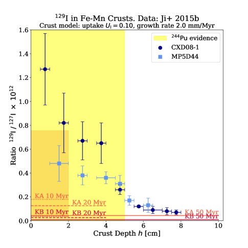
Figure 14: An example of the potential power of ${}^{129}{\rm I}$ measurements. We show an estimate of the evolution with depth of the ${}^{129}{\rm I}$/${}^{127}{\rm I}$ isotope ratio, based on the AMS data of Ji et al. (2015b). The horizontal lines represent the ratio ${}^{129}{\rm I}$/${}^{127}{\rm I}$ that would be generated within the KA and KB models occurring at the the indicated times $t_{\rm KN}$ in the past; these represent a floor below which the natural ${}^{129}{\rm I}$ background cannot fall. The KA curves for $t_{\rm KN}=(10,20)\ \rm Myr$ are off-scale. These model lines assume a crust iodine uptake $U_{\rm I}=0.1$ and a constant growth rate $\dot{h}_{0}=2\,\rm mm/Myr$. Model uncertainties for $t({\rm KB})=10\ \rm Myr$ are shown as a red band; similar ranges apply to the other cases. Model line heights scale as $U_{\rm I}\,\exp(-t_{\rm KN}/\tau_{129})$, and maximum depth scales as $h_{\rm max}=\dot{h}_{0}t_{\rm KN}$. The yellow band shows the extent of ${}^{244}{\rm Pu}$ evidence using the assumed $\dot{h}_{0}$.

The AMS measurements of ${}^{129}{\rm I}$ by Ji et al. (2015a) and Ji et al. (2015b) are from three ferromanganese crusts. For two of these, Ji et al. (2015a) tabulated ${}^{129}{\rm I}$ profiles to depths of 8 cm. Table 11 gives the locations and elemental compositions of these crusts, which are both in the mid-Pacific, at locations separated by about 2300 km. The natural production of ${}^{129}{\rm I}$ includes uranium fission products, as well as the daughters of spallation events between cosmic rays and atmospheric xenon. These give rise to a persistent flux of ${}^{129}{\rm I}$ into the crusts, which represents an irreducible background.

Ji et al. (2015a) and Ji et al. (2015b) found that the crusts show an ${}^{129}{\rm I}$/${}^{127}{\rm I}$ isotopic profile that drops with depth in a manner consistent with a background component undergoing radioactive decay, as seen in Fig. 14. Moreover, the most recent layer has an abundance consistent with the pre-bomb level found in sediments (Moran et al., 1998). Ji et al. (2015a) argue that this drop-off with depth suggests that the results are free of anthropogenic contamination. We note that the crust data show no strong evidence for a “floor” of ${}^{129}{\rm I}$ that persists as the background diminishes at increasing depth.

The crusts in which Ji et al. (2015a) measured ${}^{129}{\rm I}$ lack independent measures of their growth rates, without which the depth profile cannot be transformed into a precise time history. Nonetheless we can use typical Fe-Mn growth rates to estimate the epochs probed: for a low growth rate $\dot{h}=1\ \rm mm/Myr$, the crusts span 5–80 Myr, while a high growth rate $\dot{h}=6\ \rm mm/Myr$ would correspond to a range of 1-13 Myr. It is therefore not clear that these data include the 2-3 Mya range of the ${}^{60}{\rm Fe}$ pulse, so that the SN (one-step) scenario may not be probed directly by these data. However, as seen in Fig. 12 and Table 9, the SB model predicts ${}^{129}{\rm I}$ many orders of magnitude above the natural background, so that such a signal could be easily ruled out (or detected!) in a search coincident with the ${}^{60}{\rm Fe}$ pulses in a crust. This is the case despite the significant model uncertainties, which are indicated in Fig. 12 but omitted in Fig. 14 for clarity. On the other hand, the SA model uncertainties are large enough that their lower extreme overlaps with the KN models.

On the other hand, it is clear that these data cover the timespan probed by the extended ${}^{244}{\rm Pu}$ flux, and thus probe the two-step scenario of KN enrichment of the proto-Local Bubble. We illustrate the power of ${}^{129}{\rm I}$ data in Fe-Mn crusts using the Ji et al. (2015a) data while emphasizing that, due to the lack of information on growth rate and uptake, our quantitative results are only crude estimates. Nevertheless, we hope that such order-of-magnitude estimates may stimulate further experimental work. In this spirit, we again assume a constant growth rate $\dot{h}_{0}$, so that a time $t$ in the past corresponds to a depth $h(t)=\dot{h}_{0}\,t$. If the KN event occurred at a time $t_{\rm KN}$ ago, the signal can extend to a maximum depth $h_{\rm max}=\dot{h}_{0}\,t_{\rm KN}$.

All KN-produced radioisotopes would have decayed for the (unknown) $t_{\rm KN}$ duration since the explosion, regardless of the time history of their flux on Earth. Thus any KN-created flux will not show a radioactive decay pattern versus depth. This is in contrast to the natural ${}^{129}{\rm I}$ background, which is due to ongoing production and so should show the effects of decay versus depth. Just such a pattern is evident in Fig. 14; any KN-produced signal would represent a “floor” underneath this natural background. Thus the deepest measurements have the most constraining power.

The KN signal in the crust is straightforward to calculate in the case where the growth rate and r-process flux are both constant. In this case the ${}^{129}{\rm I}$ profile versus depth $h$ for KN model $\alpha=(\rm KA,KB)$ has a steplike structure:

$$\frac{\mbox{${}^{129}{\rm I}$}}{\mbox{${}^{127}{\rm I}$}}\left(h\right)_{\alpha}=\left\{\begin{array}[]{cl}(\mbox{${}^{129}{\rm I}$}/\mbox{${}^{127}{\rm I}$})_{\alpha,0}\ \ e^{-t_{\rm KN}/\tau_{129}}\ \ ,&h\leq h_{\rm max}=t_{\rm KN}/\dot{h}_{0}\,,\\ 0\ \ ,&h>h_{\rm max}\,,\end{array}\right.$$ (19)

where $(\mbox{${}^{129}{\rm I}$}/\mbox{${}^{127}{\rm I}$})_{\alpha,0}=N_{129}^{\alpha}/N_{127}^{\rm bg}$ from Eq. (18), which includes a factor $f_{\rm I}$ for dust formation and transport, and the uptake factor $U_{\rm I}$. We see that the isotope ratio is constant with depth, and for increasing $t_{\rm KN}$ the level is progressively smaller but extends to greater depths.

In Fig. 14 we confront the data of Ji et al. (2015a, b) with some results from calculations based on the KN models KA and KB. For each of these, we show predictions for KN explosion time $t_{\rm KN}=(10,20,50)\ \rm Myr$, corresponding to a scenario in which an explosion at this time enriches and stirs the proto-Local Bubble, initiating a flux of r-process dust onto the Earth. The ${}^{244}{\rm Pu}$ data in Fig. 7 shows that this flux extended at least to the earliest measured bin $12-25$ Mya, but neither excludes nor requires an earlier flux. Thus our constraints should apply only within this time window, though the explosion would have occurred earlier.

To predict the ${}^{129}{\rm I}$/${}^{127}{\rm I}$ ratio in the crust, we assume a constant growth rate $\dot{h}_{0}=2\ \rm mm/Myr$ and and a value $U_{\rm I}=0.1$ of the uptake factor for iodine.  With these $(\dot{h}_{0},U_{\rm I})$ values, model KA would be excluded if the KN occurred $\lesssim 50$ Mya, whereas model KB would be allowed for explosions $\gtrsim 20$ Mya. There are clearly many uncertainties in this analysis: the line heights scale as $(f_{i}/f_{\rm Pu})U_{\rm I}\,\exp(-t_{\rm KN}/\tau_{129})$ and they reach to maximum depths that scale as $h_{\rm max}=\dot{h}_{0}\;t_{\rm KN}$. Thus KA models can be accommodated with, for example, smaller uptake values.

The larger lesson is that it is of great interest to make additional ${}^{129}{\rm I}$ measurements in Fe-Mn crusts, which could offer an important new probe of possible sources of $r$-process isotopes. Also, it would be of considerable interest to search at even greater depths and thus earlier times than those shown in Fig. 19, to see if the ${}^{129}{\rm I}$ signal continues to drop as expected from a natural background, or whether a “floor” reveals itself and thereby indicates a scenario with a early injection time and thus a distant production epoch $t_{\rm KN}$. It would be of particular interest to measure ${}^{129}{\rm I}$ in crusts with ${}^{60}{\rm Fe}$ data, searching both inside and beyond the ${}^{60}{\rm Fe}$ pulses; similarly, it would be useful to search for ${}^{129}{\rm I}$ in the same crusts that show ${}^{244}{\rm Pu}$ signals. Finally, we stress that independent measures of the growth rate, and of the iodine uptake, are as important as the additional ${}^{129}{\rm I}$ data themselves. The ability to limit astrophysical perturbations to ${}^{129}{\rm I}$ hinges on the precision and reliability of the ${}^{129}{\rm I}$ profiles with time.

6.6 Lunar Searches

A great advantage of lunar material is that it avoids geological and oceanographic effects that transport, mix, and dilute the signal. Moreover, the uptake is likely to be high, so that all of the favored radioisotopes among those that can be produced via the $r$-process, namely ${}^{93}{\rm Zr}$, ${}^{107}{\rm Pd}$, ${}^{129}{\rm I}$, ${}^{135}{\rm Cs}$, ${}^{182}{\rm Hf}$, ${}^{236}{\rm U}$, ${}^{237}{\rm Np}$, ${}^{244}{\rm Pu}$, and ${}^{247}{\rm Cm}$, are a priori interesting targets for searches in the lunar regolith (i.e., unconsolidated surface material). Fry et al. (2015) cautioned that some fast dust particles could lead to the vaporization and escape of some of the ejecta mass. However, the lunar detections of ${}^{60}{\rm Fe}$ (Fimiani et al., 2016), with a fluence that is relatively high compared to terrestrial results, suggest that these effects are small. This could imply that much of the astrophysical dust slows to lower speeds by the time the particles arrive.

Thus the surface fluences of SN species should be close to the interstellar fluences estimated in Table 8, modulo a geometric factor of the cosine of the vertical angle. However, converting these values into predictions in, say, atoms per gram, requires one understands lunar surface processes over Myr timescales. Such a detailed analysis is beyond the scope of this work; we intend to visit this issue in a separate paper. Here we summarize some important considerations.

As impactors strike the lunar surface, the regolith gets continually reworked, a process known as gardening. Gardening mixes material more deeply over time, so that deeper material is less likely to have been disturbed recently, though it would have been disturbed in the more distant past. Shallow soil is continually turned over by the large flux of very small impactors. Costello et al. (2018) showed that there has been significant reworking down to $\sim$10 cm over the past 3 Myr, and significant reworking down to $\sim$40 cm over the past 400 Myr. Tables 6 and 7 suggest that ${}^{129}{\rm I}$, ${}^{236}{\rm U}$, and ${}^{244}{\rm Pu}$ may be the most interesting search targets at lower depths. However, the gardening process implies that lunar samples cannot be time-stamped accurately, and we recall that the Apollo lunar samples (Fimiani et al., 2016) have no direct timing information.

On the other hand, lunar samples may provide valuable information on the possible direction of any astrophysical source of live radioisotopes. If these arrive in dust grains that travel ballistically, their distributions could depend on the lunar latitude. The Apollo landing sites were all relatively close to the lunar equator. Therefore, in view also of their limited statistics, they provide limited information in this regard. However, the recent Chang’e-5 sample return mission landed at a higher latitude, $43.1^{o}$ N (Qian et al., 2021), the Artemis program envisions landing at the lunar south pole (Smith et al., 2020), and various commercial lunar sample return missions are also planned. More information on the latitude distribution may therefore be available in the coming years, and could discriminate between origins in the Scorpius-Centaurus (Benitez et al., 2002; Breitschwerdt et al., 2012) and Tucana-Horologium (Mamajek, 2015) associations.

Even if dust propagation is not ballistic (as suggested by Fry et al., 2020), the lunar surface distribution of radioisotopes in general offers a unique measure of the directionality of the dust velocity distribution. This directly probes SN dust propagation that is otherwise inaccessible observationally.

We note, however, that there is an important source of radioisotope background on the Moon, namely cosmic-ray spallation on the lunar surface. This is an irreducible background, so the signal must be found above it. Spallation is less important for the heaviest isotopes, and is most effective when only one or a few nucleons are removed from a target nucleus. Thus a key issue is whether there are relatively abundant stable isotopes that have one or a few more nucleons than the radioisotope of interest. We note also that, although there is no anthropogenic background on the Moon, care must be taken after bringing samples to Earth, so as to avoid anthropogenic contamination, which was an issue for the evidence for ${}^{236}{\rm U}$ and ${}^{237}{\rm Np}$ on the Moon reported by Fields et al. (1972).

Cosmic-ray irradiation of the lunar regolith also produces a substantial neutron flux at depth. Neutron exposure would lead to a ${}^{236}{\rm U}$ background that makes any extrasolar ${}^{236}{\rm U}$ difficult to find, but ${}^{236}{\rm U}$ searches could nonetheless be useful to establish which if either of these components is present. We note also that neutron captures on ${}^{236}{\rm U}$ will lead to ${}^{237}{\rm Np}$, creating a background for that species.

It is therefore encouraging that the Chang’e-5 mission has recently returned to Earth a new sample of lunar material, and that the future Artemis and other lunar missions have similar objectives. We advocate efforts to replicate the Apollo results of ${}^{60}{\rm Fe}$ and urge searches for the other radioisotopes discussed in this paper. The Apollo samples were gathered relatively close to the lunar equator, whereas Chang’e-5 landed in the northern hemisphere and Artemis is planned to land near the south pole. Measurements in their samples may therefore provide a measure of the dust arrival direction(s), and perhaps some indication of the latitude of their astrophysical sources. This would herald the dawn of radioisotope astronomy.

7 Discussion

We have found that the ${}^{244}{\rm Pu}$ detection implies that there should also be measurable traces of other r-process radioisotopes, whose abundances and time history can shed important new light. Of these, ${}^{93}{\rm Zr}$, ${}^{107}{\rm Pd}$, ${}^{135}{\rm Cs}$, and ${}^{182}{\rm Hf}$ are not only r-process species but can also be made in the s-process. Were these the only isotopes detected, this would lead to ambiguity about the nucleosynthesis site that led to their injection on Earth. But by comparing the time signature with those of ${}^{60}{\rm Fe}$ and ${}^{244}{\rm Pu}$, one can see if they are associated with the production of these isotopes. It is conceivable as well that some species such as these could arise from a recent event distinct from the origins of both the ${}^{60}{\rm Fe}$ and ${}^{244}{\rm Pu}$. For example, the s-process output of an AGB star could be delivered to Earth, perhaps via a two-step process within the proto-Local Bubble similar to what we have proposed for the KN injection of ${}^{244}{\rm Pu}$. Here again, the abundance patterns and time history of these species can test for such a model, and it would be of interest to investigate this scenario in more detail.

Our studies of live radioisotopes ejected from recent nearby explosions are closely linked with the long-studied question of now-extinct radioisotopes injected into the proto-solar nebula. As described in the excellent reviews by Meyer & Clayton (2000); Adams (2010); Lugaro et al. (2018), meteorites show evidence that more than a dozen of what we call “medium-lived” radioisotopes (“short-lived” in the cosmochemistry literature) were present in the nascent solar system. These include some r-process species (Meyer, 1993; Côté et al., 2021). Our calculations could be used to provide a new evaluation of pre-decay abundances for the early Solar System.

The discovery of ${}^{60}{\rm Fe}$ in deep-ocean deposits heralded a new era of laboratory astrophysics using relic live radioisotopes to explore events in the solar neighborhood, using them to understand quantitatively their contributions to nucleosynthesis. Previous studies have focused on nearby SNe and their roles in forming the Local Bubble. The hints of discovery of ${}^{244}{\rm Pu}$ carry these studies to a new level, including the possibility of gathering experimental information about sites of the $r$-process, extending the catalog of events of interest to include KNe, possibly out to a larger range surrounding the Local Bubble. This development also extends and expands the investigation of the potential repercussions on Earth of astrophysical events, including possible impacts on the biosphere. The longer half-life of ${}^{244}{\rm Pu}$ (81 Myr) compared to ${}^{60}{\rm Fe}$ (2.5 Myr) offers the possibility of studying the implications of such events in the more distant past, and exploring directly possible links to mass terrestrial extinctions, opening up a new frontier in astrobiology.

8 Conclusions and Future Directions

The Wallner et al. (2021) detection of a substantial ${}^{244}{\rm Pu}$ signal in the deep ocean dramatically broadens the study of near-Earth explosions, because it demands that an r-process event occurred relatively recently and close by. Indeed, ${}^{244}{\rm Pu}$ not only originates exclusively in the r process, but also is one of the heaviest nuclei it can produce. Thus the firm detection of ${}^{244}{\rm Pu}$ not only opens a new window into the elusive r-process astrophysical site(s), but also points to an engine capable of synthesizing the fullest possible complement of species, extending to actinides. The ${}^{244}{\rm Pu}$ coincidence in time with ${}^{60}{\rm Fe}$–now seen in two distinct events–suggests a common origin in SNe, yet modern SN models often struggle to host an r-process site, and typically yield no ${}^{244}{\rm Pu}$ at all. Observationally, r-process abundances in halo stars and dwarf galaxies also demand that most SNe do not make the r-process. Thus one is driven also to consider a separate event–a neutron star merger, where theoretical calculations show robust synthesis of actinides including ${}^{244}{\rm Pu}$, now supported by evidence of substantial r-process production in the GW170817 KN.

We have therefore presented pairs of SN and KN models for r-process actinide production and delivery to Earth. The former illustrate scenarios for SN actinide production in a forced neutrino-driven wind model and in an MHD model; these are adjusted to fit the data on abundances measured in the metal-poor star HD160617. We have also presented two representative KN models, with different combinations of dynamical ejecta and disk wind contributions, chosen to fit the data on HD160617 and an actinide-boost star J0954+5246. These models indicate that radioisotopes of interest with half-lives between about 1 and 100 Myr include ${}^{93}{\rm Zr}$, ${}^{107}{\rm Pd}$, ${}^{129}{\rm I}$, ${}^{135}{\rm Cs}$, and ${}^{182}{\rm Hf}$. As seen in Fig. 12, at least some of these may be detectable using AMS techniques, and their presence or non-detection could constrain significantly models of $r$-process nucleosynthesis.

The reported observations of ${}^{244}{\rm Pu}$ are nicely compatible with the the direct (one-step) deposition of explosion debris of an r-process-enhanced SN within ${\cal O}(100)$ pc of Earth, the same distance range postulated to explain the observed ${}^{60}{\rm Fe}$ signal. But most SNe do not make r-process radioisotopes and certainly not r-process actinides, so if the ${}^{244}{\rm Pu}$ had been produced by two SNe, both must be rare events (and it must be possible for some SNe to produce actinides). If instead we try to account for the ${}^{244}{\rm Pu}$ by direct (one-step) deposition by a KN, the required distances are unfeasibly large. As an alternative, we have proposed a two-step scenario, in which some of the ${}^{244}{\rm Pu}$ produced by a more distant KN was absorbed into the ISM within the Local Bubble, before subsequently reaching Earth among the debris from a nearby SN.

We now summarize our conclusions. First, we reviewed the state of present and future r-process radioisotope observations.

• We have compiled a comprehensive list of possible signatures of near-Earth explosions in the form of medium-lived radioisotopes, summarizing their possible astrophysical origins and geological prospects, and assessing their detectability via AMS. Thereafter we have focused on r-process species, and presented new calculations of r-process radioisotope yields and uncertainties for selected SN and KN scenarios constrained to reproduce solar and actinide-boosted halo star abundance patterns.

• Turning to geological data, we reviewed data on deep-ocean ${}^{244}{\rm Pu}$ in Fe-Mn crusts and sediments, combining searches by four groups. The published indications are intriguing: The published evidence for ${}^{244}{\rm Pu}$ deposits spans an extended time period from 1 to between 12 and 25 Mya. The largest fluxes overlap the times of SN ${}^{60}{\rm Fe}$ deposition, but the sustained flux over a much longer interval (if real) points toward a separate mechanism for r-process deposition on Earth.

We then performed r-process nucleosynthesis calculations, and linked them to astrophysical models for radioisotope delivery to Earth.

• We find that, for both SNe and KNe, ${}^{129}{\rm I}$ is the most abundant product, with r-process mass fractions that are comparable in the different models we address here. The production of ${}^{107}{\rm Pd}$ is similarly robust, but there are progressively larger variations in the yields of ${}^{93}{\rm Zr}$, ${}^{135}{\rm Cs}$, and ${}^{182}{\rm Hf}$. The rates of actinide production show the largest variations between the models, but their production ratios are relatively stable. Motivated by the discovery of live ${}^{244}{\rm Pu}$ in the deep ocean, we have used these observations to anchor predictions for other actinide radioisotopes.

• For SNe, we have studied r-process radioisotope production in both a forced neutrino-driven wind scenario and a magnetohydrodynamic model. These SN scenarios struggle to make actinides at all unless neutrino processes are able to create low $Y_{e}$ conditions. Thus the SN models, and particularly the unmodified MHD SN model, give high ratios of the lighter r-process radioisotopes relative to ${}^{244}{\rm Pu}$. On the other hand, KNe resulting from neutron star mergers show robust r-process actinide synthesis, and therefore have lower ratios of the lighter r-process radioisotopes relative to ${}^{244}{\rm Pu}$.

• We have studied the delivery to Earth by a nearby SN 3 Mya of ${}^{244}{\rm Pu}$ and other r-process radioisotopes along with ${}^{60}{\rm Fe}$. In this one-step model, the inferred ${}^{244}{\rm Pu}$ yields can be accommodated in both the forced neutrino-driven wind and MHD models. By contrast, such a one-step direct deposition of KN products is strongly inconsistent with both ${}^{60}{\rm Fe}$ and ${}^{244}{\rm Pu}$ data. We therefore constructed a two-step model for r-process delivery to Earth in which a KN explosion $\sim 10$ to $\sim 50$ Mya enriched the molecular cloud that gave rise to the Local Bubble. Dust grains seeded thereby with r-process radioiostopes would have bombarded the Earth thereafter. This model can account for the observed ${}^{244}{\rm Pu}$ with plausible KN distances and rates.

Finally we presented a series of predictions for specific isotope ratios and discussed their observability.

• We have presented predictions for AMS searches for r-process radioisotopes in deep-ocean Fe-Mn crusts, in both the one-step SN and two-step KN scenarios. With the current AMS sensitivities, ${}^{129}{\rm I}$ is the most promising. Potential AMS advances could make ${}^{182}{\rm Hf}$ another very interesting target. Additional AMS improvements would be needed to detect ${}^{93}{\rm Zr}$, ${}^{107}{\rm Pd}$, and ${}^{135}{\rm Cs}$. Whilst alternative production mechanisms may elevate the ${}^{236}{\rm U}$ background, measurements of ${}^{236}{\rm U}$, ${}^{237}{\rm Np}$, and ${}^{247}{\rm Cm}$ may serve as important complementary measurements to the ${}^{244}{\rm Pu}$ data.

• We have also reviewed the Moon’s fossil record of radioisotopes, where the systematics are very different from, and complementary to, those of geological searches. We recall that ${}^{60}{\rm Fe}$ has already been discovered in the Apollo samples of the lunar regolith, and have discussed opportunities for the new generation of lunar sample return missions to yield evidence for $r$-process radioisotopes.

Our work and its larger context suggest many directions for future work, which we summarize here.

Astrophysical models:

• Explosion models remain essential, and we urge that radioisotope yields be reported for calculations within models of both SNe and KNe and in studies of their r-process outputs. An improved treatment of neutrino interactions is critical, particularly for evaluating whether realistic neutrino physics allows for SN actinide production at all in the absence of jets. Similarly, more realistic SN jet models are needed to assess their ability and frequency of actinide production.

• We urge continued work on models of SN dust formation, propagation, and injection into the heliosphere. Astrophysical models of the Local Bubble are critical, and it would be of particular interest to study the effects of injection of debris from a nearby KN. To establish the broader context of the Local Bubble and recent radioisotope production, we urge continued studies of chemical evolution models for the larger solar neighborhood. Of particular importance is the distribution of radioisotopes including r-process species, as well as their variation.

Geological and lunar studies with AMS:

• We urge geological searches for r-process radioisotopes in deep-ocean Fe-Mn crusts, most pressingly ${}^{129}{\rm I}$. There is also a clear need for more sensitive searches in deep-ocean sediments for other live radioisotopes, coincident with the ${}^{60}{\rm Fe}$ pulses and the putative ${}^{244}{\rm Pu}$ signals in sediments. Improved time resolution for ${}^{244}{\rm Pu}$, including additional searches earlier than 10 Mya, is critical to determine if its flux history is coincident with or distinct from that of ${}^{60}{\rm Fe}$. Time resolution for additional radioisotopes will be similarly illuminating.

• We urge searches for r-process isotopes in the regolith samples brought to Earth recently by the Chang’e-5 lunar mission and upcoming missions including Artemis.

• We urge efforts to improve the AMS sensitivities for r-process radioisotopes, especially for ${}^{93}{\rm Zr}$, ${}^{107}{\rm Pd}$, ${}^{182}{\rm Hf}$, and ${}^{244}{\rm Pu}$.

• Probes of possible live radioisotope deposits in the more distant past would also be interesting. In particular, the end of the Devonian epoch $\sim 360$ Mya experienced an extinction event coincident with radiation UV-B damage to plant spores (Marshall et al., 2020). This could have been due to destruction of the ozone layer during cosmic-ray bombardment following an SN explosion $\sim 20$ pc away (Fields et al., 2020). ${}^{244}{\rm Pu}$ and possibly also ${}^{236}{\rm U}$ can provide evidence of an SN connection to the extinction if the event produced the r-process.

Nuclear experiments and theory:

• We look forward to new data on unstable, neutron-rich nuclides whose properties set the abundance ratios described here, from experiments at current and upcoming radioactive beam facilities such as CARIBU (Savard et al., 2008) and the $N=126$ factory (Savard et al., 2020) at ATLAS, RIBF at RIKEN (Motobayashi & Sakurai, 2012), ISAC/ARIEL at TRIUMF (Dilling et al., 2014; Willing et al., 2014), FAIR at GSI (Kester et al., 2016), and FRIB (Gade & Sherrill, 2016; Horowitz et al., 2019). 

• Some key nuclear properties—particularly those of very neutron-rich species close to the neutron drip line—will remain inaccessible to experiment for the foreseeable future. Thus, advances in nuclear structure and reaction theory will also be required to improve estimates of masses, reaction rates, and fission properties and reduce yield prediction uncertainties.

We have entered an era of multi-messenger astrophysics, with the advent of gravitational wave, cosmic ray, and neutrino measurements that complement the many decades of the electromagnetic spectrum that were already being explored. In particular, a new window into r-process nucleosynthesis opened with the simultaneous detection of a neutron star merger gravitational-wave event GW170817 and the electromagnetic discovery of the associated KN outburst (Abbott et al., 2017a, b). To these multi-messenger observations may be added the detection of live radioisotopes, which cast light not only on nucleosynthesis, but also on the history of the solar neighborhood and the potential impacts of nearby astrophysical events on the terrestrial environment and life. The first observations of deep-ocean deposits of live ${}^{60}{\rm Fe}$ have been confirmed by many other experiments, extending to measurements of ${}^{60}{\rm Fe}$ in samples of the lunar regolith, Antarctic ice, and cosmic rays. This wealth of data firmly establishes that nearby SNe occurred about 3 and 7 Myr ago, and ${}^{244}{\rm Pu}$ deposition on similar time scales has now been established.

The detection of deep-ocean ${}^{244}{\rm Pu}$ represents a novel probe of the r-process, one that is complementary to observations of neutron star mergers and stellar abundance patterns. Geophysical samples of live ${}^{244}{\rm Pu}$, and potentially other r-process radioisotopes, offer new laboratory-based probes of fresh nucleosynthesis products. These measurements are highly sensitive and isotopically specific, tied to a single nucleosynthesis event, and capable of helping us to infer the nature of the source–though only indirectly. In contrast, in neutron star merger observations the basic nature of the event is known, but the nucleosynthesis output may only be inferred indirectly and without isotopic or even elemental specificity. The abundances of r-process species in low-metallicity halo and dwarf galaxy stars offer a wealth of elemental information but generally no isotopic information. In general, stellar abundances sum over multiple synthesis events and, like geo-radioisotopes, do not directly identify the source(s). Clearly the most fruitful strategy is to use all of these r-process probes together, and now deep-ocean data contributes to this holistic approach.

References

- Abbar et al. (2021) Abbar, S., Capozzi, F., Glas, R., Janka, H. T., & Tamborra, I. 2021, Phys. Rev. D, 103, 063033, doi: 10.1103/PhysRevD.103.063033
- Abbott et al. (2017a) Abbott, B. P., et al. 2017a, Astrophys. J. Lett., 848, L12, doi: 10.3847/2041-8213/aa91c9
- Abbott et al. (2017b) —. 2017b, Astrophys. J. Lett., 848, L13, doi: 10.3847/2041-8213/aa920c
- Abbott et al. (2017) Abbott, B. P., Abbott, R., Abbott, T. D., et al. 2017, ApJ, 848, L12, doi: 10.3847/2041-8213/aa91c9
- Abbott et al. (2017) Abbott et al., B. P. 2017, Phys. Rev. Lett., 119, 161101, doi: 10.1103/PhysRevLett.119.161101
- Abt (2011) Abt, H. A. 2011, AJ, 141, 165, doi: 10.1088/0004-6256/141/5/165
- Adams (2010) Adams, F. C. 2010, ARA&A, 48, 47, doi: 10.1146/annurev-astro-081309-130830
- Adams et al. (2013) Adams, S. M., Kochanek, C. S., Beacom, J. F., Vagins, M. R., & Stanek, K. Z. 2013, ApJ, 778, 164, doi: 10.1088/0004-637X/778/2/164
- Andreoni et al. (2020) Andreoni, I., Kool, E. C., Sagués Carracedo, A., et al. 2020, ApJ, 904, 155, doi: 10.3847/1538-4357/abbf4c
- Andreoni et al. (2021) Andreoni, I., Coughlin, M. W., Kool, E. C., et al. 2021, Fast-transient Searches in Real Time with ZTFReST: Identification of Three Optically-discovered Gamma-ray Burst Afterglows and New Constraints on the Kilonova Rate. https://arxiv.org/abs/2104.06352
- Arcones & Janka (2011) Arcones, A., & Janka, H. T. 2011, A&A, 526, A160, doi: 10.1051/0004-6361/201015530
- Arcones et al. (2007) Arcones, A., Janka, H. T., & Scheck, L. 2007, A&A, 467, 1227, doi: 10.1051/0004-6361:20066983
- Arcones & Thielemann (2013) Arcones, A., & Thielemann, F. K. 2013, Journal of Physics G Nuclear Physics, 40, 013201, doi: 10.1088/0954-3899/40/1/013201
- Argast et al. (2004) Argast, D., Samland, M., Thielemann, F. K., & Qian, Y. Z. 2004, A&A, 416, 997, doi: 10.1051/0004-6361:20034265
- Arnould et al. (2007) Arnould, M., Goriely, S., & Takahashi, K. 2007, Phys. Rep., 450, 97, doi: 10.1016/j.physrep.2007.06.002
- Athanassiadou & Fields (2011) Athanassiadou, T., & Fields, B. D. 2011, New A, 16, 229, doi: 10.1016/j.newast.2010.09.007
- Audi et al. (2017) Audi, G., Kondev, F. G., Wang, M., Huang, W., & Naimi, S. 2017, Chinese Physics C, 41, 030001, doi: 10.1088/1674-1137/41/3/030001
- Balantekin & Yüksel (2005) Balantekin, A. B., & Yüksel, H. 2005, New Journal of Physics, 7, 51, doi: 10.1088/1367-2630/7/1/051
- Barnes et al. (2020) Barnes, J., Zhu, Y. L., Lund, K. A., et al. 2020, arXiv e-prints, arXiv:2010.11182. https://arxiv.org/abs/2010.11182
- Bauswein et al. (2013) Bauswein, A., Goriely, S., & Janka, H. T. 2013, ApJ, 773, 78, doi: 10.1088/0004-637X/773/1/78
- Beniamini & Hotokezaka (2020) Beniamini, P., & Hotokezaka, K. 2020, MNRAS, 496, 1891, doi: 10.1093/mnras/staa1690
- Benitez et al. (2002) Benitez, N., Maiz-Apellániz, J., & Canelles, M. 2002, Phys. Rev. Lett., 88, 081101, doi: 10.1103/PhysRevLett.88.081101
- Berghöfer & Breitschwerdt (2002) Berghöfer, T. W., & Breitschwerdt, D. 2002, A&A, 390, 299, doi: 10.1051/0004-6361:20020627
- Binns et al. (2016) Binns, W., et al. 2016, Science, 352, 677, doi: 10.1126/science.aad6004
- Blake & Schramm (1973) Blake, J. B., & Schramm, D. N. 1973, Nature Physical Science, 243, 138, doi: 10.1038/physci243138a0
- Bliss et al. (2018) Bliss, J., Witt, M., Arcones, A., Montes, F., & Pereira, J. 2018, ApJ, 855, 135, doi: 10.3847/1538-4357/aaadbe
- Bovard et al. (2017) Bovard, L., Martin, D., Guercilena, F., et al. 2017, Phys. Rev. D, 96, 124005, doi: 10.1103/PhysRevD.96.124005
- Breitschwerdt et al. (2012) Breitschwerdt, D., de Avillez, M., Feige, J., & Dettbarn, C. 2012, Astronomische Nachrichten, 333, 486, doi: https://doi.org/10.1002/asna.201211692
- Breitschwerdt et al. (2009) Breitschwerdt, D., de Avillez, M. A., & Baumgartner, V. 2009, in American Institute of Physics Conference Series, Vol. 1156, The Local Bubble and Beyond II, ed. R. K. Smith, S. L. Snowden, & K. D. Kuntz, 271–279, doi: 10.1063/1.3211826
- Breitschwerdt et al. (2016) Breitschwerdt, D., Feige, J., Schulreich, M. M., et al. 2016, Nature, 532, 73, doi: 10.1038/nature17424
- Broecker et al. (1982) Broecker, W. S., Peng, T.-H., et al. 1982, Tracers in the Sea (Lamont-Doherty Geological Observatory, Columbia University Palisades, New York)
- Burbidge et al. (1957) Burbidge, E. M., Burbidge, G. R., Fowler, W. A., & Hoyle, F. 1957, Reviews of Modern Physics, 29, 547, doi: 10.1103/RevModPhys.29.547
- Caballero et al. (2012) Caballero, O. L., McLaughlin, G. C., & Surman, R. 2012, ApJ, 745, 170, doi: 10.1088/0004-637X/745/2/170
- Chen & Beloborodov (2007) Chen, W.-X., & Beloborodov, A. M. 2007, ApJ, 657, 383, doi: 10.1086/508923
- Choplin et al. (2020) Choplin, A., Tominaga, N., & Meyer, B. S. 2020, A&A, 639, A126, doi: 10.1051/0004-6361/202037966
- Christl et al. (2014) Christl, M., Dai, X., Lachner, J., Kramer-Tremblay, S., & Synal, H.-A. 2014, Nuclear Instruments and Methods in Physics Research B, 331, 225, doi: 10.1016/j.nimb.2013.11.045
- Chruslinska et al. (2018) Chruslinska, M., Belczynski, K., Klencki, J., & Benacquista, M. 2018, MNRAS, 474, 2937, doi: 10.1093/mnras/stx2923
- Costello et al. (2018) Costello, E. S., Ghent, R. R., & Lucey, P. G. 2018, Icarus, 314, 327, doi: 10.1016/j.icarus.2018.05.023
- Côté et al. (2018) Côté, B., Fryer, C. L., Belczynski, K., et al. 2018, ApJ, 855, 99, doi: 10.3847/1538-4357/aaad67
- Côté et al. (2019) Côté, B., Eichler, M., Arcones, A., et al. 2019, ApJ, 875, 106, doi: 10.3847/1538-4357/ab10db
- Côté et al. (2021) Côté, B., Eichler, M., Yagüe López, A., et al. 2021, Science, 371, 945, doi: 10.1126/science.aba1111
- Cowan et al. (2021) Cowan, J. J., Sneden, C., Lawler, J. E., et al. 2021, Reviews of Modern Physics, 93, 015002, doi: 10.1103/RevModPhys.93.015002
- Cowan et al. (1991) Cowan, J. J., Thielemann, F.-K., & Truran, J. W. 1991, Physics Reports, 208, 267, doi: https://doi.org/10.1016/0370-1573(91)90070-3
- Cowperthwaite et al. (2017) Cowperthwaite et al., P. S. 2017, ApJL, 848, L17. http://stacks.iop.org/2041-8205/848/i=2/a=L17
- Crutcher (1982) Crutcher, R. M. 1982, ApJ, 254, 82, doi: 10.1086/159707
- Davila et al. (2019) Davila, N., Bojazi, M. J., & Meyer, B. S. 2019, in American Institute of Physics Conference Series, Vol. 2076, Exotic Nuclei and Nuclear/particle AstroPhysics (VII). Physics with Small Accelerators, 030005, doi: 10.1063/1.5091631
- Della Valle et al. (2018) Della Valle, M., Guetta, D., Cappellaro, E., et al. 2018, MNRAS, 481, 4355, doi: 10.1093/mnras/sty2541
- Dessart et al. (2009) Dessart, L., Ott, C. D., Burrows, A., Rosswog, S., & Livne, E. 2009, ApJ, 690, 1681, doi: 10.1088/0004-637X/690/2/1681
- Dilling et al. (2014) Dilling, J., Krücken, R., & Ball, G. 2014, Hyperfine Interactions, 225, 1, doi: 10.1007/s10751-013-0877-7
- Dillmann (2008) Dillmann, I. 2008, AIP Conf. Proc., 1016, 143, doi: 10.1063/1.2943564
- Duan et al. (2011) Duan, H., Friedland, A., McLaughlin, G. C., & Surman, R. 2011, Journal of Physics G Nuclear Physics, 38, 035201, doi: 10.1088/0954-3899/38/3/035201
- Eichler et al. (2015) Eichler, M., Arcones, A., Kelic, A., et al. 2015, ApJ, 808, 30, doi: 10.1088/0004-637X/808/1/30
- Ellis et al. (1996) Ellis, J., Fields, B. D., & Schramm, D. N. 1996, ApJ, 470, 1227, doi: 10.1086/177945
- Ellis & Schramm (1995) Ellis, J., & Schramm, D. N. 1995, Proceedings of the National Academy of Sciences, 92, 235, doi: 10.1073/pnas.92.1.235
- Endrizzi et al. (2016) Endrizzi, A., Ciolfi, R., Giacomazzo, B., Kastaun, W., & Kawamura, T. 2016, Classical and Quantum Gravity, 33, 164001, doi: 10.1088/0264-9381/33/16/164001
- Feige et al. (2018) Feige, J., Wallner, A., Altmeyer, R., et al. 2018, Phys. Rev. Lett., 121, 221103, doi: 10.1103/PhysRevLett.121.221103
- Fernández et al. (2015) Fernández, R., Kasen, D., Metzger, B. D., & Quataert, E. 2015, MNRAS, 446, 750, doi: 10.1093/mnras/stu2112
- Fields & Ellis (1999) Fields, B. D., & Ellis, J. 1999, New A, 4, 419, doi: 10.1016/S1384-1076(99)00034-2
- Fields et al. (2005) Fields, B. D., Hochmuth, K. A., & Ellis, J. 2005, ApJ, 621, 902, doi: 10.1086/427797
- Fields et al. (2020) Fields, B. D., Melott, A. L., Ellis, J., et al. 2020, Proceedings of the National Academy of Science, 117, 21008, doi: 10.1073/pnas.2013774117
- Fields et al. (1976) Fields, P. R., Diamond, H., Metta, D. N., & Rokop, D. J. 1976, in Lunar and Planetary Science Conference, Vol. 7, Lunar and Planetary Science Conference, 251
- Fields et al. (1972) Fields, P. R., Diamond, H., Metta, D. N., Rokop, D. J., & Stevens, C. M. 1972, Lunar and Planetary Science Conference Proceedings, 3, 1637
- Fifield et al. (1997) Fifield, L., Clacher, A., Morris, K., et al. 1997, Nuclear Instruments and Methods in Physics Research Section B: Beam Interactions with Materials and Atoms, 123, 400, doi: https://doi.org/10.1016/S0168-583X(96)00428-4
- Fimiani et al. (2016) Fimiani, L., et al. 2016, Phys. Rev. Lett., 116, 151104
- Fischer et al. (2010) Fischer, T., Whitehouse, S. C., Mezzacappa, A., Thielemann, F. K., & Liebendörfer, M. 2010, A&A, 517, A80, doi: 10.1051/0004-6361/200913106
- Fischer et al. (2020) Fischer, T., Wu, M.-R., Wehmeyer, B., et al. 2020, ApJ, 894, 9, doi: 10.3847/1538-4357/ab86b0
- Fitoussi & Raisbeck (2007) Fitoussi, C., & Raisbeck, G. M. 2007, Nuclear Instruments and Methods in Physics Research B, 259, 351, doi: 10.1016/j.nimb.2007.01.179
- Fitoussi et al. (2008) Fitoussi, C., et al. 2008, Phys. Rev. Lett., 101, 121101, doi: 10.1103/PhysRevLett.101.121101
- Foucart et al. (2015) Foucart, F., O’Connor, E., Roberts, L., et al. 2015, Phys. Rev. D, 91, 124021, doi: 10.1103/PhysRevD.91.124021
- Frisch (1981) Frisch, P. C. 1981, Nature, 293, 377, doi: 10.1038/293377a0
- Frisch et al. (2011) Frisch, P. C., Redfield, S., & Slavin, J. D. 2011, ARA&A, 49, 237, doi: 10.1146/annurev-astro-081710-102613
- Fröhlich et al. (2006) Fröhlich, C., Martinez-Pinedo, G., Liebendörfer, M., et al. 2006, Phys. Rev. Lett., 96, 142502, doi: 10.1103/PhysRevLett.96.142502
- Fry et al. (2015) Fry, B. J., Fields, B. D., & Ellis, J. R. 2015, ApJ, 800, 71, doi: 10.1088/0004-637X/800/1/71
- Fry et al. (2016) —. 2016, ApJ, 827, 48, doi: 10.3847/0004-637X/827/1/48
- Fry et al. (2020) —. 2020, ApJ, 894, 109, doi: 10.3847/1538-4357/ab86bf
- Fuchs et al. (2006) Fuchs, B., Breitschwerdt, D., de Avillez, M. A., Dettbarn, C., & Flynn, C. 2006, MNRAS, 373, 993, doi: 10.1111/j.1365-2966.2006.11044.x
- Fujimoto & Nagakura (2021) Fujimoto, S.-i., & Nagakura, H. 2021, MNRAS, 502, 2319, doi: 10.1093/mnras/stab171
- Fujimoto et al. (2008) Fujimoto, S.-i., Nishimura, N., & Hashimoto, M.-a. 2008, ApJ, 680, 1350, doi: 10.1086/529416
- Gade & Sherrill (2016) Gade, A., & Sherrill, B. M. 2016, Phys. Scripta, 91, 053003, doi: 10.1088/0031-8949/91/5/053003
- Gall et al. (2017) Gall, C., Hjorth, J., Rosswog, S., Tanvir, N. R., & Levan, A. J. 2017, ApJ, 849, L19, doi: 10.3847/2041-8213/aa93f9
- Girardi et al. (2005) Girardi, L., Groenewegen, M. A. T., Hatziminaoglou, E., & da Costa, L. 2005, A&A, 436, 895, doi: 10.1051/0004-6361:20042352
- Giuliani et al. (2020) Giuliani, S. A., Martinez-Pinedo, G., Wu, M.-R., & Robledo, L. M. 2020, Phys. Rev. C, 102, 045804, doi: 10.1103/PhysRevC.102.045804
- Gomez et al. (2012) Gomez, H. L., Clark, C. J. R., Nozawa, T., et al. 2012, MNRAS, 420, 3557, doi: 10.1111/j.1365-2966.2011.20272.x
- Goriely et al. (2009) Goriely, S., Chamel, N., & Pearson, J. M. 2009, Phys. Rev. Lett., 102, 152503, doi: 10.1103/PhysRevLett.102.152503
- Goriely & Janka (2016) Goriely, S., & Janka, H. T. 2016, MNRAS, 459, 4174, doi: 10.1093/mnras/stw946
- Gosse & Phillips (2001) Gosse, J. C., & Phillips, F. M. 2001, Quaternary Science Reviews, 20, 1475, doi: 10.1016/S0277-3791(00)00171-2
- Guozhu et al. (2013) Guozhu, H., Ming, H., Zuying, Z., et al. 2013, Nuclear Instruments and Methods in Physics Research B, 294, 132, doi: 10.1016/j.nimb.2012.05.016
- Hain et al. (2018) Hain, K., Deneva, B., Faestermann, T., et al. 2018, Nuclear Instruments and Methods in Physics Research B, 423, 42, doi: 10.1016/j.nimb.2018.02.034
- Hartmann et al. (2002) Hartmann, D. H., Kretschmer, K., & Diehl, R. 2002, in Nuclear Astrophysics, ed. W. Hillebrandt & E. Müller, 154–163. https://arxiv.org/abs/astro-ph/0205110
- Hartmann et al. (2001) Hartmann, L., Ballesteros-Paredes, J., & Bergin, E. A. 2001, ApJ, 562, 852, doi: 10.1086/323863
- Haxton & Johnson (1988) Haxton, W., & Johnson, C. W. 1988, Nature, 333, 325
- Hayakawa et al. (2018) Hayakawa, T., Ko, H., Cheoun, M.-K., et al. 2018, Phys. Rev. Lett., 121, 102701, doi: 10.1103/PhysRevLett.121.102701
- Hein et al. (2000) Hein, J. R., Koschinsky, A., Bau, M., et al. 2000, Handbook of marine mineral deposits, 18, 239
- Hoffman et al. (1971) Hoffman, D. C., Lawrence, F. O., Mewherter, J. L., & Rourke, F. M. 1971, Nature, 152, 132
- Hoffman et al. (1997) Hoffman, R. D., Woosley, S. E., & Qian, Y. Z. 1997, ApJ, 482, 951, doi: 10.1086/304181
- Holmbeck et al. (2018) Holmbeck, E. M., Beers, T. C., Roederer, I. U., et al. 2018, ApJ, 859, L24, doi: 10.3847/2041-8213/aac722
- Horowitz et al. (2019) Horowitz, C. J., Arcones, A., Côté, B., et al. 2019, Journal of Physics G Nuclear Physics, 46, 083001, doi: 10.1088/1361-6471/ab0849
- Hotokezaka et al. (2013) Hotokezaka, K., Kiuchi, K., Kyutoku, K., et al. 2013, Phys. Rev. D, 87, 024001, doi: 10.1103/PhysRevD.87.024001
- Howard (1993) Howard, W. M. 1993, Meteoritics, 28, 365
- Hüdepohl et al. (2010) Hüdepohl, L., Müller, B., Janka, H. T., Marek, A., & Raffelt, G. G. 2010, Phys. Rev. Lett., 104, 251101, doi: 10.1103/PhysRevLett.104.251101
- Hunter (2007) Hunter, J. D. 2007, Computing in Science and Engineering, 9, 90, doi: 10.1109/MCSE.2007.55
- Ji et al. (2015a) Ji, L., Liu, G., Chen, Z., et al. 2015a, Acta Oceanologica Sinica, 34, 31
- Ji et al. (2015b) Ji, L., Liu, G., Huang, Y., Xing, N., & Chen, Z. 2015b, Acta Oceanologica Sinica, 34, 13
- Jin et al. (2018) Jin, Z.-P., Li, X., Wang, H., et al. 2018, ApJ, 857, 128, doi: 10.3847/1538-4357/aab76d
- Johns et al. (2020) Johns, L., Nagakura, H., Fuller, G. M., & Burrows, A. 2020, Phys. Rev. D, 102, 103017, doi: 10.1103/PhysRevD.102.103017
- Just et al. (2015) Just, O., Bauswein, A., Ardevol Pulpillo, R., Goriely, S., & Janka, H. T. 2015, MNRAS, 448, 541, doi: 10.1093/mnras/stv009
- Just et al. (2015) Just, O., Bauswein, A., Pulpillo, R. A., Goriely, S., & Janka, H.-T. 2015, Monthly Notices of the Royal Astronomical Society, 448, 541, doi: 10.1093/mnras/stv009
- Kajino et al. (2019) Kajino, T., Aoki, W., Balantekin, A., et al. 2019, Progress in Particle and Nuclear Physics, 107, 109, doi: https://doi.org/10.1016/j.ppnp.2019.02.008
- Kasen et al. (2017) Kasen, D., Metzger, B., Barnes, J., Quataert, E., & Ramirez-Ruiz, E. 2017, Nature, 551, 80, doi: 10.1038/nature24453
- Kester et al. (2016) Kester, O., Spiller, P., & Stoecker, H. 2016, FAIR project at GSI, 611–622, doi: 10.1142/9789814436403_0032
- Knie et al. (1999) Knie, K., Korschinek, G., Faestermann, T., et al. 1999, Phys. Rev. Lett., 83, 18, doi: 10.1103/PhysRevLett.83.18
- Knie et al. (2004) Knie, K., et al. 2004, Phys. Rev. Lett., 93, 171103
- Kobayashi et al. (2020) Kobayashi, C., Karakas, A. I., & Lugaro, M. 2020, ApJ, 900, 179, doi: 10.3847/1538-4357/abae65
- Kodama & Takahashi (1975) Kodama, T., & Takahashi, K. 1975, Nuclear Physics A, 239, 489, doi: https://doi.org/10.1016/0375-9474(75)90381-4
- Koll et al. (2019) Koll, D., Korschinek, G., Faestermann, T., et al. 2019, Phys. Rev. Lett., 123, 072701, doi: 10.1103/PhysRevLett.123.072701
- Kondev et al. (2021) Kondev, F. G., Wang, M., Huang, W. J., Naimi, S., & Audi, G. 2021, Chinese Physics C, 45, 030001, doi: 10.1088/1674-1137/abddae
- Korobkin et al. (2020) Korobkin, O., Hungerford, A. M., Fryer, C. L., et al. 2020, ApJ, 889, 168, doi: 10.3847/1538-4357/ab64d8
- Korschinek et al. (1994) Korschinek, G., Faestermann, T., Kastel, S., et al. 1994, Nuclear Instruments and Methods in Physics Research B, 92, 146, doi: 10.1016/0168-583X(94)95995-1
- Korschinek et al. (2020) Korschinek, G., Faestermann, T., Poutivtsev, M., et al. 2020, Phys. Rev. Lett., 125, 031101, doi: 10.1103/PhysRevLett.125.031101
- Kutschera (2013) Kutschera, W. 2013, International Journal of Mass Spectrometry, 349-350, 203, doi: 10.1016/j.ijms.2013.05.023
- Kyutoku & Ioka (2016) Kyutoku, K., & Ioka, K. 2016, ApJ, 827, 83, doi: 10.3847/0004-637X/827/1/83
- Kyutoku et al. (2018) Kyutoku, K., Kiuchi, K., Sekiguchi, Y., Shibata, M., & Taniguchi, K. 2018, Phys. Rev. D, 97, 023009, doi: 10.1103/PhysRevD.97.023009
- Lachner et al. (2012) Lachner, J., Dillmann, I., Faestermann, T., et al. 2012, Phys. Rev. C, 85, 015801, doi: 10.1103/PhysRevC.85.015801
- Lazauskas et al. (2009) Lazauskas, R., Lunardini, C., & Volpe, C. 2009, JCAP, 04, 029, doi: 10.1088/1475-7516/2009/04/029
- Lehner et al. (2016) Lehner, L., Liebling, S. L., Palenzuela, C., et al. 2016, Classical and Quantum Gravity, 33, 184002, doi: 10.1088/0264-9381/33/18/184002
- Lien & Fields (2009) Lien, A., & Fields, B. D. 2009, J. Cosmology Astropart. Phys, 2009, 047, doi: 10.1088/1475-7516/2009/01/047
- Lindahl et al. (2005) Lindahl, P., Roos, P., Holm, E., & Dahlgaard, H. 2005, Journal of Environmental Radioactivity, 82, 285, doi: https://doi.org/10.1016/j.jenvrad.2005.01.011
- Looney et al. (2006) Looney, L. W., Tobin, J. J., & Fields, B. D. 2006, ApJ, 652, 1755, doi: 10.1086/508407
- López-Lora & Chamizo (2019) López-Lora, M., & Chamizo, E. 2019, Nuclear Instruments and Methods in Physics Research B, 455, 39, doi: 10.1016/j.nimb.2019.06.018
- Ludwig et al. (2016) Ludwig, P., Bishop, S., Egli, R., et al. 2016, Proceedings of the National Academy of Sciences, 113, 9232, doi: 10.1073/pnas.1601040113
- Lugaro et al. (2018) Lugaro, M., Ott, U., & Kereszturi, Á. 2018, Progress in Particle and Nuclear Physics, 102, 1, doi: 10.1016/j.ppnp.2018.05.002
- Maiz-Apellaniz (2001) Maiz-Apellaniz, J. 2001, ApJ, 560, L83, doi: 10.1086/324016
- Malkus et al. (2016) Malkus, A., McLaughlin, G. C., & Surman, R. 2016, Phys. Rev. D, 93, 045021, doi: 10.1103/PhysRevD.93.045021
- Mamajek (2015) Mamajek, E. E. 2015, Proceedings of the International Astronomical Union, 10, 21–26, doi: 10.1017/S1743921315006250
- Marketin et al. (2016) Marketin, T., Huther, L., & Martinez-Pinedo, G. 2016, Phys. Rev. C, 93, 025805, doi: 10.1103/PhysRevC.93.025805
- Marshall et al. (2020) Marshall, J. E., Lakin, J., Troth, I., & Wallace-Johnson, S. M. 2020, Science Advances, 6, eaba0768
- Martin et al. (2015) Martin, D., Perego, A., Arcones, A., et al. 2015, ApJ, 813, 2, doi: 10.1088/0004-637X/813/1/2
- Martschini et al. (2019) Martschini, M., Fifield, L. K., Froehlich, M. B., et al. 2019, Nuclear Instruments and Methods in Physics Research Section B: Beam Interactions with Materials and Atoms, 438, 141, doi: https://doi.org/10.1016/j.nimb.2018.05.039
- Martschini et al. (2020) Martschini, M., Lachner, J., Merchel, S., et al. 2020, in European Physical Journal Web of Conferences, Vol. 232, European Physical Journal Web of Conferences, 02003, doi: 10.1051/epjconf/202023202003
- Masarik & Beer (1999) Masarik, J., & Beer, J. 1999, J. Geophys. Res., 104, 12099, doi: 10.1029/1998JD200091
- Matteucci et al. (2014) Matteucci, F., Romano, D., Arcones, A., Korobkin, O., & Rosswog, S. 2014, MNRAS, 438, 2177, doi: 10.1093/mnras/stt2350
- McGary & Johnson (2007) McGary, V. T., & Johnson, C. W. 2007, Astropart. Phys., 27, 233, doi: 10.1016/j.astropartphys.2006.10.002
- McLaughlin et al. (1999) McLaughlin, G. C., Fetter, J. M., Balantekin, A. B., & Fuller, G. M. 1999, Phys. Rev. C, 59, 2873, doi: 10.1103/PhysRevC.59.2873
- Melott et al. (2019) Melott, A. L., Marinho, F., & Paulucci, L. 2019, Astrobiology, 19, 825, doi: 10.1089/ast.2018.1902
- Melott et al. (2004) Melott, A. L., Lieberman, B. S., Laird, C. M., et al. 2004, International Journal of Astrobiology, 3, 55, doi: 10.1017/S1473550404001910
- Meyer (1993) Meyer, B. S. 1993, Meteoritics, 28, 399
- Meyer & Clayton (2000) Meyer, B. S., & Clayton, D. D. 2000, Space Sci. Rev., 92, 133, doi: 10.1023/A:1005282825778
- Miller et al. (2020) Miller, J. M., Sprouse, T. M., Fryer, C. L., et al. 2020, ApJ, 902, 66, doi: 10.3847/1538-4357/abb4e3
- Moran et al. (1998) Moran, J. E., Fehn, U., & Teng, R. T. 1998, Chemical Geology, 152, 193
- Mösta et al. (2018) Mösta, P., Roberts, L. F., Halevi, G., et al. 2018, ApJ, 864, 171, doi: 10.3847/1538-4357/aad6ec
- Motobayashi & Sakurai (2012) Motobayashi, T., & Sakurai, H. 2012, Progress of Theoretical and Experimental Physics, 2012, 03C001, doi: 10.1093/ptep/pts059
- Mumpower et al. (2018) Mumpower, M. R., Kawano, T., Sprouse, T. M., et al. 2018, ApJ, 869, 14, doi: 10.3847/1538-4357/aaeaca
- Murphey et al. (2020) Murphey, C., Hogan, J. W., Fields, B. D., & Narayan, G. 2020, arXiv e-prints, arXiv:2012.06552. https://arxiv.org/abs/2012.06552
- Murray (2011) Murray, N. 2011, ApJ, 729, 133, doi: 10.1088/0004-637X/729/2/133
- Nishimura et al. (2018) Nishimura, N., Rauscher, T., Hirschi, R., et al. 2018, Mon. Not. Roy. Astron. Soc., 474, 3133, doi: 10.1093/mnras/stx3033
- Nozaki (2001) Nozaki, Y. 2001, Encyclopedia of Ocean Sciences (eds. JH Steel et al.). Vol. 2, Academic Press
- Nozawa et al. (2011) Nozawa, T., Maeda, K., Kozasa, T., et al. 2011, ApJ, 736, 45, doi: 10.1088/0004-637X/736/1/45
- Oliphant (2006) Oliphant, T. 2006, NumPy: A guide to NumPy, USA: Trelgol Publishing. http://www.numpy.org/
- Ouellette et al. (2009) Ouellette, N., Desch, S. J., Bizzarro, M., et al. 2009, Geochim. Cosmochim. Acta, 73, 4946, doi: 10.1016/j.gca.2008.10.044
- Paresce (1984) Paresce, F. 1984, AJ, 89, 1022, doi: 10.1086/113598
- Paul et al. (2001) Paul, M., Valenta, A., Ahmad, I., et al. 2001, ApJ, 558, L133, doi: 10.1086/323617
- Pavetich et al. (2019) Pavetich, S., Carey, A., Fifield, L. K., et al. 2019, Nuclear Instruments and Methods in Physics Research B, 438, 77, doi: 10.1016/j.nimb.2018.07.019
- Perego et al. (2014) Perego, A., Rosswog, S., Cabezón, R. M., et al. 2014, MNRAS, 443, 3134, doi: 10.1093/mnras/stu1352
- Pruet et al. (2003) Pruet, J., Woosley, S. E., & Hoffman, R. D. 2003, ApJ, 586, 1254, doi: 10.1086/367957
- Qian et al. (2021) Qian, Y., Xiao, L., Wang, Q., et al. 2021, Earth and Planetary Science Letters, 561, 116855, doi: https://doi.org/10.1016/j.epsl.2021.116855
- Radice et al. (2018) Radice, D., Perego, A., Hotokezaka, K., et al. 2018, ApJ, 869, L35, doi: 10.3847/2041-8213/aaf053
- Raisbeck et al. (2007) Raisbeck, G., Tran, T., Lunney, D., et al. 2007, Nuclear Instruments and Methods in Physics Research B, 259, 673, doi: 10.1016/j.nimb.2007.01.205
- Reichert et al. (2021) Reichert, M., Obergaulinger, M., Eichler, M., Aloy, M. Á., & Arcones, A. 2021, MNRAS, 501, 5733, doi: 10.1093/mnras/stab029
- Roberts et al. (2012) Roberts, L. F., Reddy, S., & Shen, G. 2012, Phys. Rev. C, 86, 065803, doi: 10.1103/PhysRevC.86.065803
- Roederer & Lawler (2012) Roederer, I. U., & Lawler, J. E. 2012, ApJ, 750, 76, doi: 10.1088/0004-637X/750/1/76
- Röllin et al. (2009) Röllin, S., Sahli, H., Holzer, R., Astner, M., & Burger, M. 2009, Applied Radiation and Isotopes, 67, 821, doi: https://doi.org/10.1016/j.apradiso.2009.01.041
- Rosswog et al. (2017) Rosswog, S., Feindt, U., Korobkin, O., et al. 2017, Classical and Quantum Gravity, 34, 104001, doi: 10.1088/1361-6382/aa68a9
- Rosswog et al. (2013) Rosswog, S., Piran, T., & Nakar, E. 2013, Monthly Notices of the Royal Astronomical Society, 430, 2585, doi: 10.1093/mnras/sts708
- Ruderman (1974) Ruderman, M. A. 1974, Science, 184, 1079, doi: 10.1126/science.184.4141.1079
- Savard et al. (2020) Savard, G., Brodeur, M., Clark, J. A., Knaack, R. A., & Valverde, A. A. 2020, Nuclear Instruments and Methods in Physics Research B, 463, 258, doi: 10.1016/j.nimb.2019.05.024
- Savard et al. (2008) Savard, G., Baker, S., Davids, C., et al. 2008, Nuclear Instruments and Methods in Physics Research B, 266, 4086, doi: 10.1016/j.nimb.2008.05.091
- Scalo & Wheeler (2002) Scalo, J., & Wheeler, J. C. 2002, ApJ, 566, 723, doi: 10.1086/338329
- Schneider & Livingston (1984) Schneider, D., & Livingston, H. 1984, Nuclear Instruments and Methods in Physics Research, 223, 510, doi: https://doi.org/10.1016/0167-5087(84)90700-2
- Schulreich et al. (2017) Schulreich, M. M., Breitschwerdt, D., Feige, J., & Dettbarn, C. 2017, Astron. Astrophys., 604, A81, doi: 10.1051/0004-6361/201629837
- Seeger & Schramm (1970) Seeger, P. A., & Schramm, D. N. 1970, ApJ, 160, L157, doi: 10.1086/180550
- Sekiguchi et al. (2016) Sekiguchi, Y., Kiuchi, K., Kyutoku, K., Shibata, M., & Taniguchi, K. 2016, Phys. Rev. D, 93, 124046, doi: 10.1103/PhysRevD.93.124046
- Shetye et al. (2020) Shetye, S., et al. 2020, Astronomy & Astrophysics, 635, L6, doi: doi.org/10.1051/0004-6361/202037481
- Shibagaki et al. (2016) Shibagaki, S., Kajino, T., Mathews, G. J., et al. 2016, ApJ, 816, 79, doi: 10.3847/0004-637X/816/2/79
- Siegel et al. (2019) Siegel, D. M., Barnes, J., & Metzger, B. D. 2019, Nature, 569, 241, doi: 10.1038/s41586-019-1136-0
- Siegel et al. (2019) Siegel, D. M., Barnes, J., & Metzger, B. D. 2019, Nature, 569, 241, doi: 10.1038/s41586-019-1136-0
- Siegel & Metzger (2018) Siegel, D. M., & Metzger, B. D. 2018, ApJ, 858, 52, doi: 10.3847/1538-4357/aabaec
- Smith et al. (2020) Smith, M., Craig, D., Herrmann, N., et al. 2020, in 2020 IEEE Aerospace Conference, 1–10, doi: 10.1109/AERO47225.2020.9172323
- Smith & Cox (2001) Smith, R. K., & Cox, D. P. 2001, ApJS, 134, 283, doi: 10.1086/320850
- Sprouse et al. (2020) Sprouse, T. M., Mumpower, M. R., & Surman, R. 2020, arXiv e-prints, arXiv:2008.06075. https://arxiv.org/abs/2008.06075
- Steier et al. (2013) Steier, P., Hrnecek, E., Priller, A., et al. 2013, Nuclear Instruments and Methods in Physics Research Section B: Beam Interactions with Materials and Atoms, 294, 160, doi: https://doi.org/10.1016/j.nimb.2012.06.017
- Surman et al. (2006) Surman, R., McLaughlin, G. C., & Hix, W. R. 2006, ApJ, 643, 1057, doi: 10.1086/501116
- Surman et al. (2008) Surman, R., McLaughlin, G. C., Ruffert, M., Janka, H.-T., & Hix, W. R. 2008, The Astrophysical Journal, 679, L117, doi: 10.1086/589507
- Takami et al. (2014) Takami, H., Nozawa, T., & Ioka, K. 2014, ApJ, 789, L6, doi: 10.1088/2041-8205/789/1/L6
- Thompson (1982) Thompson, R. C. 1982, Radiation Research, 90, 1. http://www.jstor.org/stable/3575792
- Tsujimoto et al. (2017) Tsujimoto, T., Yokoyama, T., & Bekki, K. 2017, ApJ, 835, L3, doi: 10.3847/2041-8213/835/1/L3
- van der Walt et al. (2011) van der Walt, S., Colbert, S. C., & Varoquaux, G. 2011, Computing in Science and Engineering, 13, 22, doi: 10.1109/MCSE.2011.37
- Vassh et al. (2020) Vassh, N., Mumpower, M. R., McLaughlin, G. C., Sprouse, T. M., & Surman, R. 2020, ApJ, 896, 28, doi: 10.3847/1538-4357/ab91a9
- Vassh et al. (2019) Vassh, N., Vogt, R., Surman, R., et al. 2019, Journal of Physics G Nuclear Physics, 46, 065202, doi: 10.1088/1361-6471/ab0bea
- Vockenhuber et al. (2015) Vockenhuber, C., Casacuberta, N., Christl, M., & Synal, H.-A. 2015, Nuclear Instruments and Methods in Physics Research B, 361, 445, doi: 10.1016/j.nimb.2015.01.061
- Vockenhuber et al. (2004) Vockenhuber, C., Oberli, F., Bichler, M., et al. 2004, Phys. Rev. Lett., 93, 172501, doi: 10.1103/PhysRevLett.93.172501
- Vockenhuber et al. (2004) Vockenhuber, C., Feldstein, C., Paul, M., et al. 2004, New Astronomy Reviews, 48, 161
- Wallner et al. (2015) Wallner, A., Faestermann, T., Feige, J., et al. 2015, Nature Communications, 6, 5956, doi: 10.1038/ncomms6956
- Wallner et al. (2016) Wallner, A., et al. 2016, Nature, 532, 69, doi: 10.1038/nature17196
- Wallner et al. (2020) Wallner, A., Feige, J., Fifield, L. K., et al. 2020, Proceedings of the National Academy of Science, 117, 21873, doi: 10.1073/pnas.1916769117
- Wallner et al. (2021) Wallner, A., et al. 2021, Science, 372, 742, doi: DOI: 10.1126/science.aax3972
- Wallner et al. (2004) Wallner, C., Faestermann, T., Gerstmann, U., et al. 2004, New A Rev., 48, 145, doi: 10.1016/j.newar.2003.11.020
- Wanajo (2006) Wanajo, S. 2006, ApJ, 650, L79, doi: 10.1086/508568
- Wanajo (2013) —. 2013, ApJ, 770, L22, doi: 10.1088/2041-8205/770/2/L22
- Wanajo et al. (2001) Wanajo, S., Kajino, T., Mathews, G. J., & Otsuki, K. 2001, ApJ, 554, 578, doi: 10.1086/321339
- Wanajo et al. (2014) Wanajo, S., Sekiguchi, Y., Nishimura, N., et al. 2014, ApJ, 789, L39, doi: 10.1088/2041-8205/789/2/L39
- Wang et al. (2020a) Wang, X., N3AS Collaboration, Fields, B. D., et al. 2020a, ApJ, 893, 92, doi: 10.3847/1538-4357/ab7ffd
- Wang et al. (2020b) Wang, X., N3AS Collaboration, Vassh, N., et al. 2020b, ApJ, 903, L3, doi: 10.3847/2041-8213/abbe18
- Wehmeyer et al. (2015) Wehmeyer, B., Pignatari, M., & Thielemann, F. K. 2015, MNRAS, 452, 1970, doi: 10.1093/mnras/stv1352
- Wilcken et al. (2008) Wilcken, K., Fifield, L., Barrows, T., Tims, S., & Gladkis, L. 2008, Nuclear Instruments and Methods in Physics Research Section B: Beam Interactions with Materials and Atoms, 266, 3614, doi: https://doi.org/10.1016/j.nimb.2008.06.009
- Willing et al. (2014) Willing, J., Krücken, R., & Merminga, L. 2014, Hyperfine Interactions, 225, 253, doi: 10.1007/s10751-013-0906-6
- Winkler et al. (2004) Winkler, S., Ahmad, I., Golser, R., et al. 2004, New A Rev., 48, 151, doi: 10.1016/j.newar.2003.11.021
- Winteler et al. (2012) Winteler, C., Käppeli, R., Perego, A., et al. 2012, ApJ, 750, L22, doi: 10.1088/2041-8205/750/1/L22
- Xiong et al. (2020) Xiong, Z., Sieverding, A., Sen, M., & Qian, Y.-Z. 2020, ApJ, 900, 144, doi: 10.3847/1538-4357/abac5e
- Yamazaki et al. (2021) Yamazaki, Y., Kajino, T., Mathews, G. J., et al. 2021, arXiv e-prints, arXiv:2102.05891. https://arxiv.org/abs/2102.05891
- Yan et al. (2019) Yan, Y., Bender, M. L., Brook, E. J., et al. 2019, Nature, 574, 663 , doi: 10.1038/s41586-019-1692-3
- Yin et al. (2015) Yin, X., He, M., Dong, K., et al. 2015, Nuclear Instruments and Methods in Physics Research B, 361, 488, doi: 10.1016/j.nimb.2015.07.124
- Yong et al. (2021) Yong, D., Kobayashi, C., Da Costa, G. S., et al. 2021, Nature, 595, 223, doi: 10.1038/s41586-021-03611-2
- Zhu et al. (2018) Zhu, Y., Wollaeger, R. T., Vassh, N., et al. 2018, ApJ, 863, L23, doi: 10.3847/2041-8213/aad5de
- Zhu et al. (2021) Zhu, Y. L., Lund, K. A., Barnes, J., et al. 2021, ApJ, 906, 94, doi: 10.3847/1538-4357/abc69e