TAG: Task-based Accumulated Gradients for Lifelong learning

Abstract

When an agent encounters a continual stream of new tasks in the lifelong learning setting, it leverages the knowledge it gained from the earlier tasks to help learn the new tasks better. In such a scenario, identifying an efficient knowledge representation becomes a challenging problem. Most research works propose to either store a subset of examples from the past tasks in a replay buffer, dedicate a separate set of parameters to each task or penalize excessive updates over parameters by introducing a regularization term. While existing methods employ the general task-agnostic stochastic gradient descent update rule, we propose a task-aware optimizer that adapts the learning rate based on the relatedness among tasks. We utilize the directions taken by the parameters during the updates by additively accumulating the gradients specific to each task. These task-based accumulated gradients act as a knowledge base that is maintained and updated throughout the stream. We empirically show that our proposed adaptive learning rate not only accounts for catastrophic forgetting but also exhibits knowledge transfer. We also show that our method performs better than several state-of-the-art methods in lifelong learning on complex datasets. Moreover, our method can also be combined with the existing methods and achieve substantial improvement in performance.

1 Introduction

Lifelong learning (LLL), also known as continual learning, is a setting where an agent continuously learns from data belonging to different tasks (Parisi et al., 2019). Here, the goal is to maximize performance on all the tasks arriving in a stream without replaying the entire datasets from past tasks (Riemer et al., 2018). Approaches proposed in this setting involve investigating the stability-plasticity dilemma (Mermillod et al., 2013) in different ways where stability refers to preventing the forgetting of past knowledge and plasticity refers to accumulating new knowledge by learning new tasks (Mermillod et al., 2013; Delange et al., 2021).

Unlike human beings, who can efficiently assess the correctness and applicability of the past knowledge (Chen & Liu, 2018), neural networks and other machine learning models often face various issues in this setting. Whenever data from a new task arrives, these models often tend to forget the previously obtained knowledge due to dependency on the input data distribution, limited capacity, diversity among tasks, etc. This leads to a significant drop in performance on the previous tasks - also known as catastrophic forgetting (McCloskey & J. Cohen, 1989; Robins, 1993; Xie et al., 2021).

Recently there has been an ample amount of research proposed in LLL (Delange et al., 2021). Several methods, categorized as Parameter Isolation methods, either freeze or add a set of parameters as their task knowledge when a new task arrives. Another type of methods, known as Regularization-based methods, involve an additional regularization term to tackle the stability-plasticity dilemma (Kirkpatrick et al., 2017; Li et al., 2021). There are approaches based on approximate Bayesian inference, where parameters are sampled from a distribution, that suggest controlling the updates based on parameter uncertainty (Blundell et al., 2015; Adel et al., 2019; Ahn et al., 2019). But these approaches are computationally expensive and often depend on the choice of prior (Zenke et al., 2017; Nguyen et al., 2018).

Another class of methods, namely Replay-based methods, store a subset of examples from each task in a replay buffer. These methods apply gradient-based updates that facilitate a high-level transfer across different tasks through the examples from the past tasks that are simultaneously available while training. As a result, these methods tend to frame LLL as an i.i.d. setting (Bang et al., 2021; Saha et al., 2021). While replay-based methods are currently state-of-the-art in several LLL tasks, it is important that we explore various ways to tackle the original non-i.i.d. problem (Hadsell et al., 2020). Hence the focus of this paper is to design efficient replay-free methods for LLL.

While adaptive gradient descent based optimizers such as Adam (Kingma & Ba, 2014) have shown superior performance in the classical machine learning setup, many existing works in LLL employ the conventional stochastic gradient descent for parameter update (Lopez-Paz & Ranzato, 2017; Chaudhry et al., 2019; Farajtabar et al., 2020). Adaptive gradient descent based optimizers accumulate gradients to regulate the magnitude and direction of updates but often struggle when the dataset arrives in a non-i.i.d. manner, from different tasks, etc. These optimizers tend to ‘over-adapt’ on the most recent batch and hence suffer from poor generalization performance (Keskar & Socher, 2017; Chen et al., 2018; Mirzadeh et al., 2020).

While exploiting the adaptive nature of the gradient descent based optimizers, we alleviate catastrophic forgetting by introducing Task-based Accumulated Gradients (TAG) that is a wrapper around existing optimizers. The key contributions of our work are as follows: (i) We define a task-aware adaptive learning rate for the parameter update step that is also aware of relatedness among tasks in LLL. (ii) As the knowledge base, we propose to additively accumulate the directions (or gradients) that the network took while learning a specific task instead of storing past examples. (iii) We empirically show that our method prevents catastrophic forgetting and exhibits knowledge transfer if the tasks are related without introducing more parameters.

Our proposed method, described in Section 3, achieves state-of-the-art results and outperforms several Replay-free methods on complex datasets like Split-miniImageNet, Split-CUB, etc. For smaller episodic memory, our method also outperforms the Replay-based methods as shown in Section 4. Note that we propose a new approach to optimizing based on the past gradients and as such it could potentially be applied along with the existing LLL methods including replay-based methods. We demonstrate the effectiveness of doing the same in the experiments.

2 Related Work

Methods proposed in LLL are broadly categorized into three classes: Regularization-based, Parameter Isolation and Replay-based methods (Masana et al., 2020; Delange et al., 2021; Mai et al., 2022). Regularization-based methods prevent a drastic change in the network parameters as the new task arrives to mitigate forgetting. These methods further are classified as data-focused (Li & Hoiem, 2017; Triki et al., 2017; Li et al., 2021) and prior-focused methods (Nguyen et al., 2018; Ebrahimi et al., 2019). In particular, Elastic Weight Consolidation (EWC) (Kirkpatrick et al., 2017), a prior-focused method, regularizes the loss function to minimize changes in the parameters important for previous tasks. Yet, when the model needs to adapt to a large number of tasks, the interference between task-based knowledge is inevitable with fixed model capacity. Parameter Isolation methods (Rusu et al., 2016; Xu & Zhu, 2018; Serra et al., 2018) such as (Aljundi et al., 2017) assign a model copy to every new task that arrives. These methods alleviate catastrophic forgetting in general, but they rely on a strong base network and work on a small number of tasks. Another closely related methods, called Expansion-based methods, handle the LLL problem by expanding the model capacity in order to adapt to new tasks (Sodhani et al., 2018; Rao et al., 2019). Replay-based methods maintain an ‘episodic memory’, containing a few examples from past tasks, that is revisited while learning a new task (Riemer et al., 2018; Jin et al., 2020). For instance, Averaged Gradient Episodic Memory (A-GEM) (Chaudhry et al., 2018b), alleviating computational inefficiency of GEM (Lopez-Paz & Ranzato, 2017), uses the episodic memory to project the gradients based on hard constraints defined on the episodic memory and the current mini-batch. Experience Replay (ER) (Chaudhry et al., 2019) uses both replay memory and input mini-batches in the optimization step by averaging their gradients to mitigate forgetting. On the other hand, we propose a replay-free method that maintains a fixed-capacity model during training and test time.

Task-relatedness (Li & Hoiem, 2017; Jerfel et al., 2019; Shaker et al., 2020) or explicitly learning task representations (Yoon et al., 2017) is also an alternative approach studied in LLL. Efficient Lifelong Learning Algorithm (ELLA) (Ruvolo & Eaton, 2013) maintains sparsely shared basis vectors for all the tasks and refines them whenever the model sees a new task. Rao et al. (2019) perform dynamic expansion of the model while learning task-specific representation and task inference within the model. Orthogonal Gradient Descent (OGD) (Farajtabar et al., 2020) maintains a space based on a subset of gradients from each task. As a result, OGD often faces memory issues during run-time depending upon the size of the model and the subset (Bennani & Sugiyama, 2020). Unlike OGD, we accumulate the gradients and hence alleviate the memory requirements by orders for each task.

A recent work (Mirzadeh et al., 2020) argues that tuning the hyper-parameters gives a better result than several state-of-the-art methods including A-GEM and ER. They introduce Stable SGD that involves an adjustment in the hyper-parameters like initial learning rate, learning rate decay, dropout, and batch size. They present this gain in performance on simplistic benchmarks like Permuted MNIST (Goodfellow et al., 2013), Rotated MNIST and Split-CIFAR100 (Mirzadeh et al., 2020). Another related work (Gupta et al., 2020) discusses a similar technique of using learning rate with episodic memory to reflect the similarities between the old and new tasks. On the other hand, our method explicitly computes the similarities between the tasks to regulate the learning rate.

3 Method

3.1 Lifelong learning Setup

In this section, we introduce the notations and the LLL setup used in the paper. We focus on the standard task-incremental learning scenario which is adopted in the numerous state-of-the-art LLL methods. It involves solving new tasks using an artificial neural network with a multi-head output where each head is associated with a unique task and the task identity is known beforehand (Lopez-Paz & Ranzato, 2017; van de Ven & Tolias, 2019; Delange et al., 2021). We denote the current task as $t$ and any of the previous tasks by $\tau$. The model receives new data of the form $\{X^{(t)},D^{(t)},Y^{(t)}\}$ where $X^{(t)}$ are the input features, $D^{(t)}$ is the task descriptor (that is a natural number in this work) and $Y^{(t)}$ is the target vector specific to the task $t$.

We consider the ‘single-pass per task’ setting in this work following (Lopez-Paz & Ranzato, 2017; Riemer et al., 2018; Chaudhry et al., 2019) where the model is trained only for one epoch on the dataset. It is more challenging than the multiple pass setting used in numerous research works (Kirkpatrick et al., 2017; Rebuffi et al., 2017). The goal is to learn a classification model $f(X^{(t)};\theta)$, parameterized by $\theta\in\mathbb{R}^{P}$ to minimize the loss $L(f(X^{(t)};\theta),Y^{(t)})$ for the current task $t$ while preventing the loss on the past tasks from increasing. We evaluate the model on a held-out set of examples of all the tasks ($\leq t$) seen in the stream.

3.2 Task-based accumulated gradients

The specific form of our proposed method depends on the underlying adaptive optimizer. For ease of exposition, we describe it as a modification of RMSProp (Tieleman & Hinton, 2012) here and call it TAG-RMSProp. The TAG versions of other methods such as the Adagrad (Duchi et al., 2011) and Adam are available in Appendix A.1. A Naive RMSProp update, for a given learning rate $\eta$, looks like the following:

$$\begin{split}V_{n}&=\beta V_{n-1}+(1-\beta)g^{2}_{n};~{}~{}1\leq n\leq N\\ \theta_{n+1}&=\theta_{n}-\frac{\eta}{\sqrt{V_{n}+\epsilon}}g_{n}\end{split}$$ (1)

where $\theta_{n}$ is the parameter vector at step $n$ in the epoch, $g_{n}$ is the gradient of the loss, $N$ is the total number of steps in one epoch, $V_{n}$ is the moving average of the square of gradients (or the second moment), and $\beta$ is the decay rate. We will use TAG-optimizers as a generic terminology for the rest of the paper.

We maintain the second moment $V^{(t)}_{n}$ for each task $t$ in the stream and store it as the knowledge base. When the model shifts from one task to another, the new loss surface may look significantly different. We argue that by using the task-based second moment to regulate the new task updates, we can reduce the interference with the previously optimized parameters in the model. We define the second moment $V^{(t)}_{n}$ for task $t$ for TAG-RMSProp as: $V^{(t)}_{n}=\beta_{2}V^{(t)}_{n-1}+(1-\beta_{2})g^{2}_{n}$ where $\beta_{2}$ is constant throughout the stream. We use $\textbf{V}^{(t)}_{n}$ to denote a matrix that stores the second moments from all previous tasks, i.e., $\textbf{V}^{(t)}_{n}=\{V^{(1)}_{N},...,V^{(t-1)}_{N},V^{(t)}_{n}\}$ of size $(t\times P)$. Hence, the memory required to store these task-specific accumulated gradients increases linearly as the number of tasks in the setting.

Note that each $V^{(\tau)}_{N}(\text{where}~{}\tau<t)$ vector captures the gradient information when the model receives data from a task $\tau$ and does not change after the task $\tau$ is learned. It helps in regulating the magnitude of the update while learning the current task $t$. To alleviate the catastrophic forgetting problem occurring in the Naive RMSProp, we replace $V_{n}$ (in Eq. 1) to a weighted sum of $\textbf{V}^{(t)}_{n}$. We propose a way to regulate the weights corresponding to $\textbf{V}^{(t)}_{n}$ for each task in the next section.

3.3 Adaptive Learning Rate

Next, we describe our proposed learning rate that adapts based on the relatedness among tasks. We discuss how task-based accumulated gradients can help regulate the parameter updates to minimize catastrophic forgetting and transfer knowledge.

We first define a representation for each task to enable computing correlation between different tasks. We take inspiration from a recent work (Guiroy et al., 2019) which is based on a popular meta-learning approach called Model-Agnostic Meta-Learning (MAML) (Finn et al., 2017). Guiroy et al. (2019) suggest that with reference to given parameters $\theta^{s}$ (where $s$ denotes shared parameters), the similarity between the adaptation trajectories (and also meta-test gradients) among the tasks can act as an indicator of good generalization. This similarity is defined by computing the inner dot product between adaptation trajectories. In the experiments, Guiroy et al. (2019) show an improvement in the overall target accuracy by adding a regularization term in the outer loop update to enhance the similarity.

In the case of LLL, instead of a fixed point of reference $\theta^{s}$, the parameters continue to update as the model adapts to a new task. Analogous to the adaptation trajectories, we essentially want to capture those task-specific gradient directions in the LLL setting. Momentum serves as a less noisy estimate for the overall gradient direction and hence approximating the adaptation trajectories. The role of momentum has been crucial in the optimization literature for gradient descent updates (Ruder, 2016; Li et al., 2017). Therefore, we introduce the task-based first moment $M^{(t)}_{n}$ in order to approximate the adaptation trajectories of each task $t$. It is essentially the momentum maintained while learning each task $t$ and would act as the task representation for computing the correlation.

The $M^{(t)}_{n}$ is defined as: $M^{(t)}_{n}=\beta_{1}M^{(t)}_{n-1}+(1-\beta_{1})g_{n}$ where $\beta_{1}$ is the constant decay rate. Intuitively, if the current task $t$ is correlated with a previous task $\tau$, the learning rate in the parameter update step should be higher to encourage the transfer of knowledge between task $t$ and $\tau$. In other words, it should allow knowledge transfer. Whereas if the current task $t$ is uncorrelated or negatively correlated to a previous task $\tau$, the new updates over parameters may cause catastrophic forgetting because these updates for task $t$ may point in the opposite direction of the previous task $\tau$’s updates. In such a case, the learning rate should adapt to lessen the effects of the new updates. We introduce a scalar quantity $\alpha_{n}(t,\tau)$ to capture the correlation that is computed using $M^{(t)}_{n}$ and $M^{(\tau)}_{N}$:

$$\alpha_{n}(t,\tau) =exp\left(-b~{}\frac{{M_{n}^{(t)}}^{T}M^{(\tau)}_{N}}{|M_{n}^{(t)}||M^{(\tau)}_{N}|}\right)$$ (2)

where $|.|$ is the Euclidean norm. Existing adaptive optimizers, such as Adam, tend to overfit on the most recent dataset from a task, which results in catastrophic forgetting in LLL. By using the exponential term, the resulting $\alpha_{n}(t,\tau)$ will attain a higher value for uncorrelated tasks and will minimize the new updates (hence prevent forgetting). Here, $b$ is a hyperparameter that tunes the magnitude of $\alpha_{n}(t,\tau)$. The higher the $b$ is, the greater is the focus on preventing catastrophic forgetting. Its value can vary for different datasets. For the current task $t$ at step $n$ (with $\theta^{(t)}_{1}=\theta^{(t-1)}_{N+1}$), we define the TAG-RMSProp update as:

$$\theta^{(t)}_{n+1} =\theta^{(t)}_{n}-\frac{\eta}{\sqrt{\alpha_{n}(t,t)~{}V^{(t)}_{n}+\sum\limits_{\tau=1}^{t-1}\alpha_{n}(t,\tau)~{}V^{(\tau)}_{N}+\epsilon}}g_{n}$$ (3)

Hence, the role of each $\alpha_{n}(t,\tau)$ is to regulate the influence of corresponding task-based accumulated gradient $V^{(\tau)}_{N}$ of the previous task $\tau$. Since we propose a new way of looking at the gradients, our update rule (Eq. 3) can be applied with any kind of task-incremental learning setup. In this way, the overall structure of the algorithm for this setup remains the same.

4 Experiments

We describe the experiments performed to evaluate our proposed method. In the first experiment, we show the gain in performance by introducing TAG update instead of naive optimizers update. We analyse how our proposed learning rate adapts and achieves a higher accuracy over the tasks in the stream. Next, we compare our proposed replay-free method with other state-of-the-art baselines and also show that TAG update (in Eq. 3) can be used along with other state-of-the-art methods to improve their results.

The experiments are performed on four benchmark datasets: Split-CIFAR100, Split-miniImageNet, Split-CUB and 5-dataset. Split-CIFAR100 and Split-miniImageNet splits the CIFAR-100 (Krizhevsky et al., 2009; Mirzadeh et al., 2020) and Mini-imagenet (Vinyals et al., 2016; Chaudhry et al., 2019) datasets into 20 disjoint 5-way classification tasks. Split-CUB splits the CUB (Wah et al., 2011) dataset into 20 disjoint tasks with 10 classes per task. 5-dataset is a sequence of five different datasets as five 10-way classification tasks. These datasets are: CIFAR-10 (Krizhevsky et al., 2009), MNIST (LeCun, 1998), SVHN (Netzer et al., 2011), notMNIST (Bulatov, 2011) and Fashion-MNIST (Xiao et al., 2017). More details about the datasets are given in Appendix A.2. For experiments with Split-CIFAR100 and Split-miniImageNet, we use a reduced ResNet18 architecture following (Lopez-Paz & Ranzato, 2017; Chaudhry et al., 2019). We use the same reduced ResNet18 architecture for 5-dataset. For Split-CUB, we use a ResNet18 model which is pretrained on Imagenet dataset (Deng et al., 2009) as used in (Chaudhry et al., 2019).

We report the following metrics by evaluating the model on the held-out test set: (i) Accuracy (Lopez-Paz & Ranzato, 2017) i.e., average test accuracy when the model has been trained sequentially up to the latest task, (ii) Forgetting (Chaudhry et al., 2018a) i.e., decrease in performance of each task from their peak accuracy to their accuracy after training on the latest task and (iii) Learning Accuracy (LA) (Riemer et al., 2018) i.e., average accuracy for each task immediately after it is learned. The overall goal is to maximise the average test Accuracy. Further, a LLL algorithm should also achieve high LA while maintaining a low value of Forgetting because it should learn the new task better without compromising its performance on the previous tasks (see Appendix A.2).

We report the above metrics on the best hyper-parameter combination obtained from a grid-search. The overall implementation of the above setting is based on the code provided by (Mirzadeh et al., 2020). The details of the grid-search and other implementation details corresponding to all experiments described in our paper are given in Appendix A.2.1. For all the experiments described in this section, we train the model for a single epoch per task. Results for multiple epochs per task are given in Appendix A.3.4. All the performance results reported are averaged over five runs.

4.1 Naive optimizers

We validate the improvement by our proposed setting over the gradient descent based methods and demonstrate the impact of using correlation among tasks in the TAG-optimizers. Firstly, we train the model on a stream of tasks using Naive SGD update without applying any specific LLL method. Similarly, we replace the SGD update with Naive Adagrad, Naive RMSProp, Naive Adam and their respective TAG-optimizers to compare their performances. We show the resulting Accuracy (%) (in Fig. 1(a)) and Forgetting (in Fig. 1(b)) when the model is trained in with the above-mentioned optimizers.

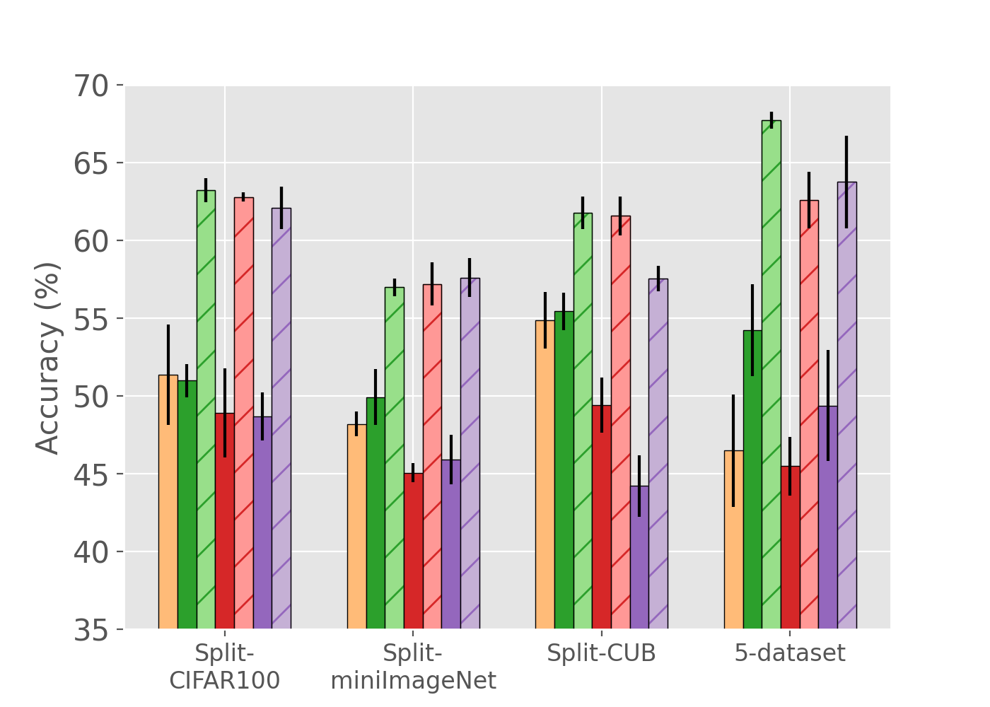
(a) Accuracy (%)

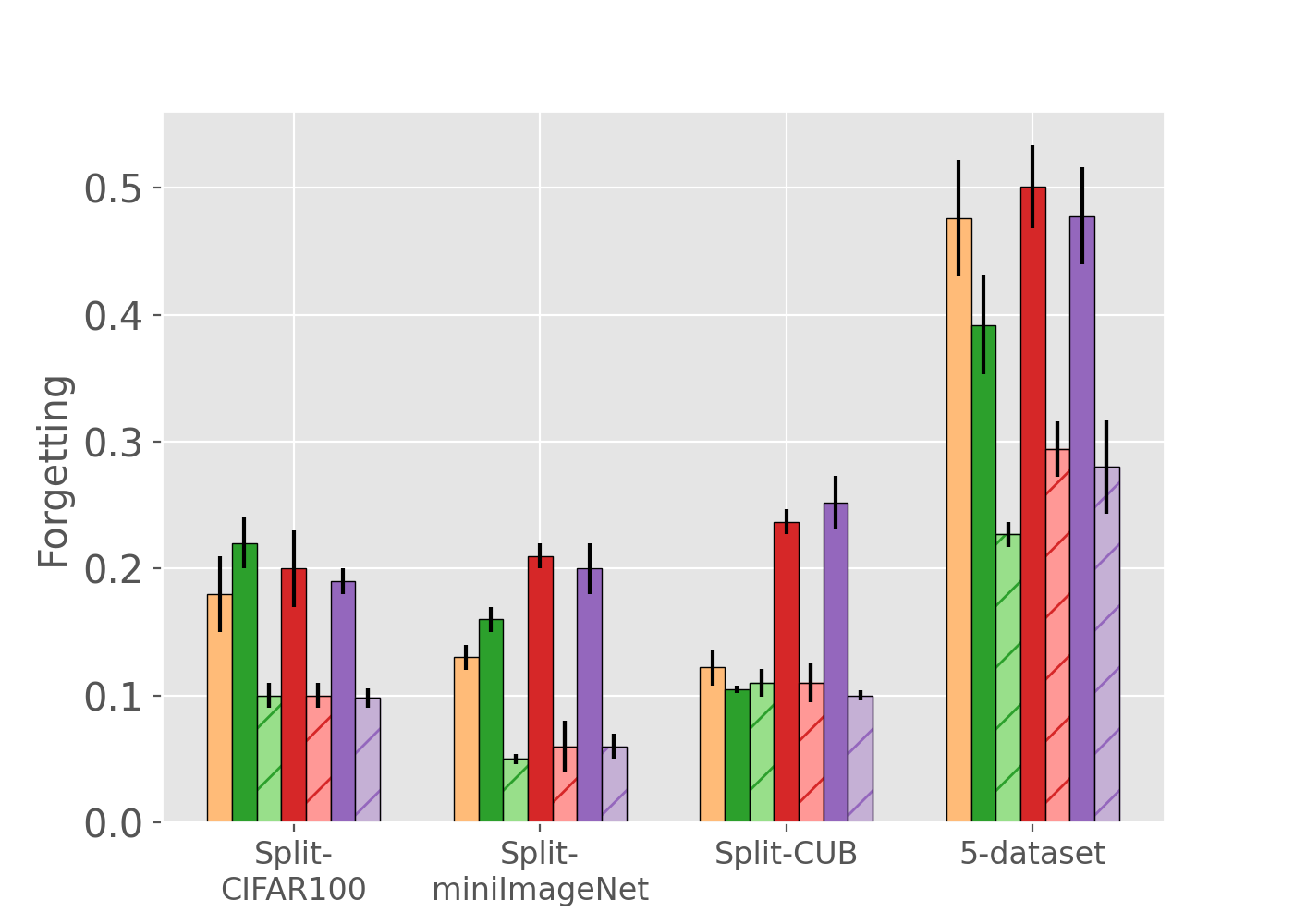
(b) Forgetting

Figure 1: Final average test Accuracy (%) (higher is better) and Forgetting (lower is better) obtained after the stream is finished for all four datasets. The vertical bars with hatches are the performance by TAG-optimizers while others are Naive optimizers. TAG-optimizers outperforms the naive optimizers in all datasets in terms of accuracy and also results in a lower forgetting.

It is clear that TAG-optimizers outperform their naive counterparts as well as Naive SGD for all four datasets by a significant amount. There is a notable decrease in Forgetting by TAG-optimizers (in Fig. 1(b)) in general that eventually reflects on the gain in final test Accuracy as seen in Fig. 1(a). In Split-CUB, TAG-Adam ($57\%$) shows a remarkable improvement in accuracy when compared to Naive Adam ($45\%$) such that it even surpasses Naive SGD ($55\%$). Interestingly, TAG-Adam results in slightly lower accuracy as compared to TAG-Adagrad except in Split-miniImageNet. Moreover, Naive Adagrad results in a better performance than Naive RMSProp and Naive Adam for all the datasets. This observation aligns with the results by Hsu et al. (2018). Naive SGD performs almost equivalent to Naive Adagrad except in 5-dataset where it is outperformed.

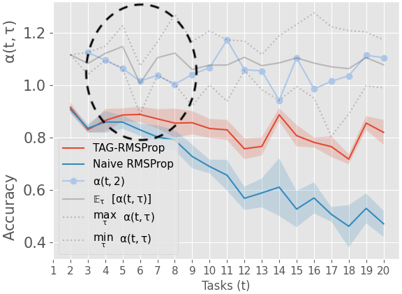
(a) $\tau=2$

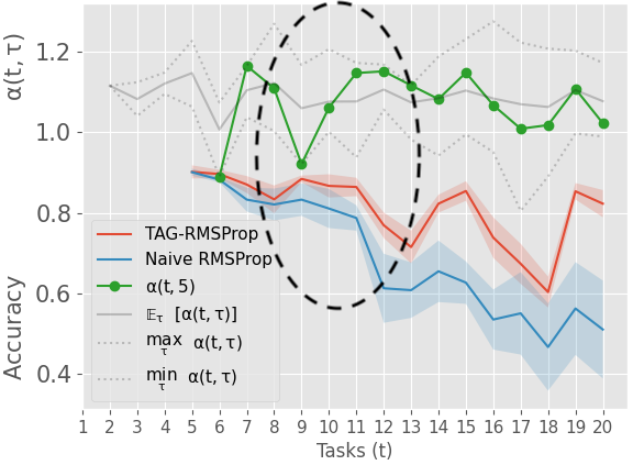
(b) $\tau=5$

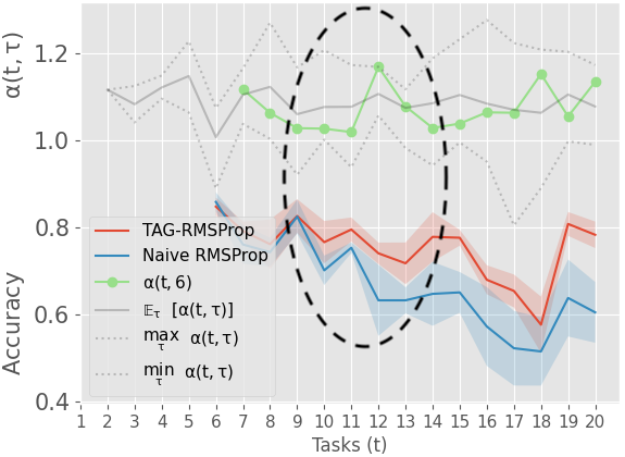
(c) $\tau=6$

Figure 2: Evolution of (a) $\alpha(t,2)$ and test accuracy $a_{t,2}$ (left), (b) $\alpha(t,5)$ and test accuracy $a_{t,5}$ (middle) and (c) $\alpha(t,6)$ and test accuracy $a_{t,6}$ (right) along the stream of $20$ tasks in the Split-CUB dataset. The grey-coloured lines are $\max_{\tau^{\prime}}\alpha_{n}(t,\tau^{\prime})$ (top, dashed line), $\mathbb{E}_{\tau^{\prime}}[\alpha(t,\tau^{\prime})]$ (middle, solid line) and $\min_{\tau^{\prime}}\alpha(t,\tau^{\prime})$ (bottom, dashed line) that indicate the range of $\alpha(t,\tau^{\prime})$. Elliptical regions (black dashed) highlight subtle gain in the accuracy by TAG-RMSProp that are maintained throughout the stream. Observing corresponding $\alpha(t,\tau)$ in those regions validates our hypothesis discussed from Section 3.3.

Next, we analyse $\alpha(t,\tau)$ which is the average of $\alpha_{n}(t,\tau)$ across all steps $n$ for all $t$ and $\tau$ when stream is finished i.e., $\alpha(t,\tau)=\frac{1}{N}\sum_{n=1}^{N}\alpha_{n}(t,\tau)$. We show how $\alpha(t,\tau)$ values play role in the gain in TAG-optimizers accuracies in case of Split-CUB dataset. Each plot in Fig. 2 corresponds to test accuracies $a_{t,\tau}$ (with shaded areas indicating their standard deviations) for Naive RMSProp (blue) and TAG-RMSProp (red) for a particular $\tau$ for all tasks $t$ in the stream (x-axis). Along with that, the grey-coloured curves are $\max_{\tau^{\prime}}\alpha_{n}(t,\tau^{\prime})$ (top, dashed line), $\mathbb{E}_{\tau^{\prime}}[\alpha(t,\tau^{\prime})]$ (middle, solid line) and $\min_{\tau^{\prime}}\alpha(t,\tau^{\prime})$ (bottom, dashed line) respectively. These curves are shown along with the corresponding $\alpha(t,\tau)$ to indicate the rank of $\alpha(t,\tau)$ in the set $\{\alpha(t,\tau^{\prime});~{}\tau^{\prime}\in[1,t]\}$. This set is computed when the model encounters the task $t$ in the stream.

The accuracies of TAG-RMSProp and Naive RMSProp appear to correlate for most of the stream. We mark the regions (black dashed ellipse) of subtle improvements in the accuracy by TAG-RMSProp that is later maintained throughout the stream. While observing $\alpha(t,\tau)$ in those regions particularly, we note that the rank of $\alpha(t,\tau)$ affects the accuracy in TAG-RMSProp as following: (i) Lower (or decrease in) rank of $\alpha(t,\tau)$ means that there exists some correlation between the tasks $t$ and $\tau$. So, the model should take advantage of the current task updates and seek (or even amplify) backward transfer. Such observations can be made for the following $(t,\tau)$: $(4,2)$, $(5,2)$, $(14,2)$, $(9,5)$, $(14,6)$, $(19,6)$ etc. Our method also prevents drastic forgetting as well in few cases. For example: $(7,2)$, $(12,2)$, $(10,6)$. (ii) Higher (or increase in) rank of $\alpha(t,\tau)$ results in prevention of forgetting as observed in Fig. 2. Such $(t,\tau)$ pairs are $(11,2)$, $(7,5)$, $(12,5)$, $(12,6)$, etc. It also results in backward transfer as observed in $(11,5)$ and $(15,5)$. We report the same analysis for the other three datasets and show the results in Appendix A.3.3.

4.2 Compared with other baselines

Table 1: Comparing performance in terms of final average test Accuracy (%) (higher is better), Forgetting (lower is better) and Learning Accuracy (LA (%)) (higher is better) of the existing baselines with TAG-RMSProp on all four datasets. All metrics are averaged across 5 runs. Overall, TAG-RMSProp outperforms all other methods in terms of Accuracy. *MTL assumes that the whole dataset from all tasks is always available during training, hence it is a different setting and its accuracy acts as an upper bound.

Methods	Split-CIFAR100			Split-miniImageNet
	Accuracy (%)	Forgetting	LA (%)	Accuracy (%)	Forgetting	LA (%)
Naive SGD	$51.36~{}(\pm 3.21)$	$0.18~{}(\pm 0.03)$	$68.46~{}(\pm 1.93)$	$48.19~{}(\pm 0.79)$	$0.13~{}(\pm 0.01)$	$60.6~{}(\pm 0.95)$
Naive RMSProp	$48.91~{}(\pm 2.88)$	$0.2~{}(\pm 0.03)$	$67.28~{}(\pm 0.43)$	$45.06~{}(\pm 0.6)$	$0.21~{}(\pm 0.01)$	$64.39~{}(\pm 1.02)$
EWC	$49.06~{}(\pm 3.44)$	$0.19~{}(\pm 0.04)$	$66.82~{}(\pm 1.41)$	$47.87~{}(\pm 2.08)$	$0.15~{}(\pm 0.02)$	$61.66~{}(\pm 1.06)$
A-GEM	$54.25~{}(\pm 2.0)$	$0.16~{}(\pm 0.03)$	$68.98~{}(\pm 1.19)$	$50.32~{}(\pm 1.29)$	$0.11~{}(\pm 0.02)$	$61.02~{}(\pm 0.64)$
ER	$59.14~{}(\pm 1.77)$	$0.12~{}(\pm 0.02)$	$70.36~{}(\pm 1.23)$	$54.67~{}(\pm 0.71)$	$0.1~{}(\pm 0.01)$	$64.06~{}(\pm 0.41)$
Stable SGD	$57.04~{}(\pm 1.07)$	$0.09~{}(\pm 0.0)$	$64.62~{}(\pm 0.91)$	$51.81~{}(\pm 1.66)$	$0.09~{}(\pm 0.01)$	$59.99~{}(\pm 0.94)$
TAG-RMSProp (Ours)	$\textbf{62.79}~{}(\pm 0.29)$	$0.1~{}(\pm 0.01)$	$72.06~{}(\pm 1.01)$	$\textbf{57.2}~{}(\pm 1.37)$	$0.06~{}(\pm 0.02)$	$62.73~{}(\pm 0.61)$
MTL*	$67.7~{}(\pm 0.58)$	-	-	$66.14~{}(\pm 1.0)$	-	-

Methods	Split-CUB			5-dataset
	Accuracy (%)	Forgetting	LA (%)	Accuracy (%)	Forgetting	LA (%)
Naive SGD	$54.88~{}(\pm 1.83)$	$0.12~{}(\pm 0.01)$	$65.97~{}(\pm 0.59)$	$46.48~{}(\pm 3.62)$	$0.48~{}(\pm 0.05)$	$84.55~{}(\pm 1.06)$
Naive RMSProp	$49.4~{}(\pm 1.77)$	$0.24~{}(\pm 0.01)$	$71.76~{}(\pm 0.94)$	$45.49~{}(\pm 1.89)$	$0.5~{}(\pm 0.03)$	$85.58~{}(\pm 1.21)$
EWC	$55.66~{}(\pm 0.97)$	$0.12~{}(\pm 0.01)$	$66.36~{}(\pm 0.71)$	$48.58~{}(\pm 1.47)$	$0.4~{}(\pm 0.03)$	$79.56~{}(\pm 3.18)$
A-GEM	$56.91~{}(\pm 1.37)$	$0.1~{}(\pm 0.01)$	$65.6~{}(\pm 0.73)$	$55.9~{}(\pm 2.58)$	$0.34~{}(\pm 0.04)$	$82.61~{}(\pm 2.13)$
ER	$59.25~{}(\pm 0.82)$	$0.1~{}(\pm 0.01)$	$66.17~{}(\pm 0.42)$	$61.58~{}(\pm 2.65)$	$0.28~{}(\pm 0.04)$	$84.3~{}(\pm 1.08)$
Stable SGD	$53.76~{}(\pm 2.14)$	$0.11~{}(\pm 0.01)$	$62.15~{}(\pm 1.12)$	$46.51~{}(\pm 2.75)$	$0.46~{}(\pm 0.03)$	$83.3~{}(\pm 1.44)$
TAG-RMSProp (Ours)	$\textbf{61.58}~{}(\pm 1.24)$	$0.11~{}(\pm 0.01)$	$71.56~{}(\pm 0.74)$	$\textbf{62.59}~{}(\pm 1.82)$	$0.29~{}(\pm 0.02)$	$86.08~{}(\pm 0.55)$
MTL*	$71.65~{}(\pm 0.76)$	-	-	$70.0~{}(\pm 4.44)$	-	-

In the next experiment, we show that the TAG-RMSProp results in a strong performance as compared to other LLL algorithms. In Table 1, we report the performance of TAG-RMSProp and the following state-of-the-art baselines: EWC (Kirkpatrick et al., 2017), A-GEM (Chaudhry et al., 2018b), ER (Aljundi et al., 2019) with reservoir sampling and Stable SGD (Mirzadeh et al., 2020). Additional details about our implementation are given in Appendix A.2. Apart from these baselines, we report the performance of Naive SGD and Naive RMSProp from the previous section. We also report results on multi-task learning (MTL) settings on all four datasets where the dataset from all the tasks is always available throughout the stream. Hence, the resulting accuracies of the MTL setting serve as the upper bounds for the test accuracies in LLL. Following Mirzadeh et al. (2020), the size of the episodic memory for both A-GEM and ER is set to store $1$ example per class. Since we want to evaluate TAG with all other baselines on the original non-i.i.d. problem, we keep the episodic memory size in the replay-based methods small for the comparison. We still report A-GEM and ER results with bigger memory sizes in Appendix A.3.5. The size of the mini-batch sampled from the episodic memory is set equal to the batch-size to avoid data imbalance while training.

Other baselines such as OGD (Farajtabar et al., 2020) requires storing N (=$200$ in their experiments) number of gradients per task and it is evaluated only on variants of the MNIST dataset by training a small feed-forward network. On the other hand, TAG additively accumulates the gradients and hence requires memory equal to two copies of the model as the knowledge base. This enabled us to train a reduced ResNet18 on complex datasets. Due to greater memory requirements, OGD faced memory errors in our setting. We would also like to highlight that OGD use Naive-SGD, whereas TAG, being an adaptive learning rate based method, is complementary to this approach. Although we utilize a similar amount of memory as Progressive Neural Networks Rusu et al. (2016), an expansion-based method, we do not make any changes to the size of the model during the training and testing process. On the other hand, Rusu et al. (2016) require quadratic growth in the number of parameters as the number of tasks increases. Hence, we do not compare our approach with the expansion-based method in our experiments.

From the results reported in Table 1, we observe that TAG-RMSProp achieves the best performance in terms of test Accuracy as compared to other baselines for all datasets. The overall improvement is decent in Split-CIFAR100, Split-miniImageNet and Split-CUB which are $3.65\%$, $2.5\%$ and $2.3\%$ with regard to the next-best baseline. On the other hand, the improvement by TAG-RMSProp is relatively minor in 5-dataset i.e., $1\%$ as compared to ER with the similar amount of Forgetting ($0.29$ and $0.28$) occurring in the stream. In terms of LA, TAG-RMSProp achieves almost similar performance as Naive RMSProp in Split-CUB and 5-dataset. We also note that the LA of TAG-RMSProp is higher in Split-CIFAR100, Split-CUB and 5-dataset than ER and A-GEM. The higher LA with similar Forgetting as compared to other baselines shows that while TAG exploits the adaptive nature of existing optimizers, it also ensures minimal forgetting of the gained knowledge. The existing optimizers tend to aggressively fit the model on the most recent task at an immense cost of forgetting the earlier tasks. Hence, even if a similar (or lower) Forgetting occurs in TAG, the higher test Accuracy (with high LA) shows that TAG is capable of retaining the gained knowledge from each task. Although LA is lower in Split-miniImageNet, TAG-RMSProp manages to prevent catastrophic forgetting better than these methods and hence results in a higher test Accuracy.

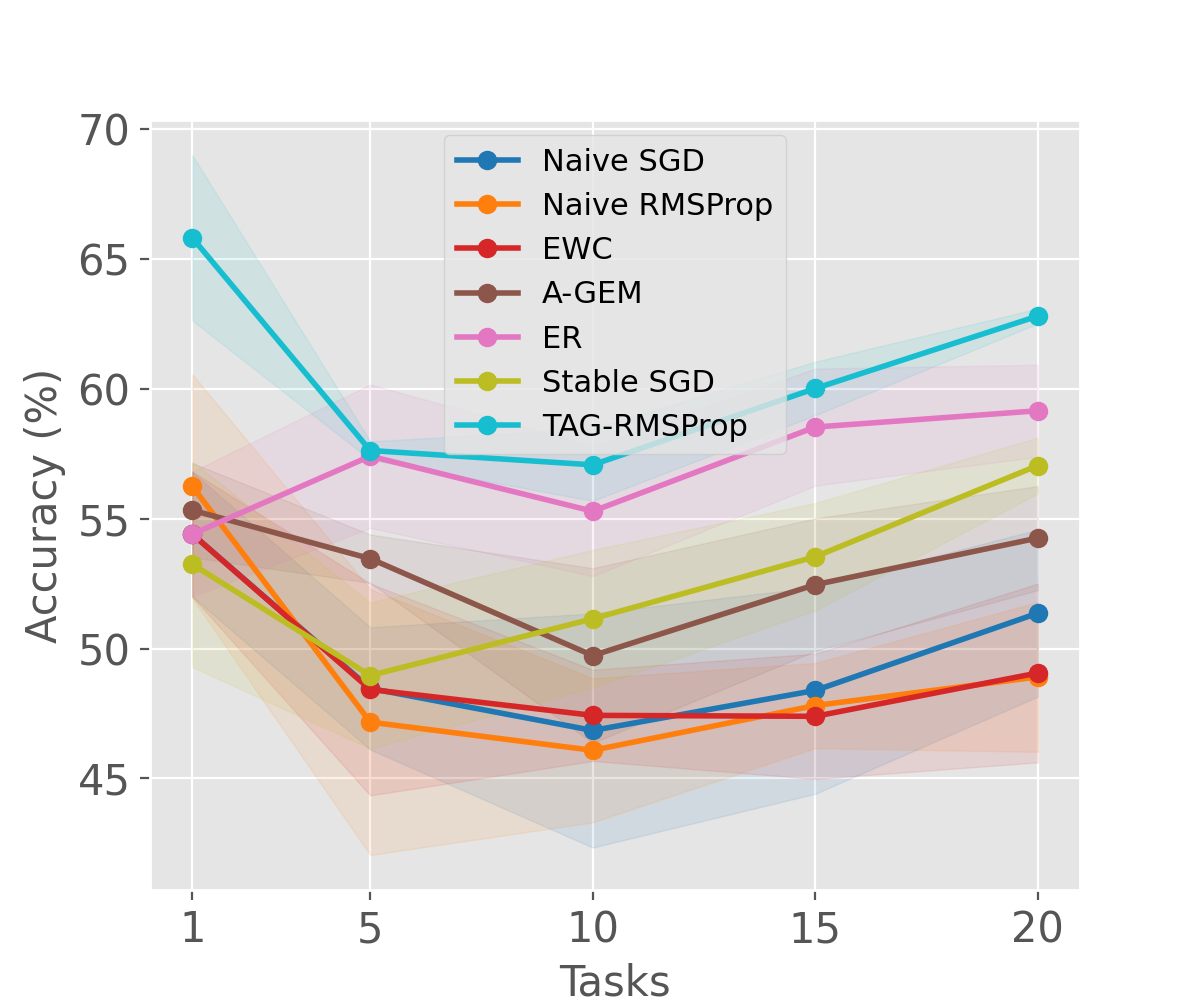
(a) Split-CIFAR100

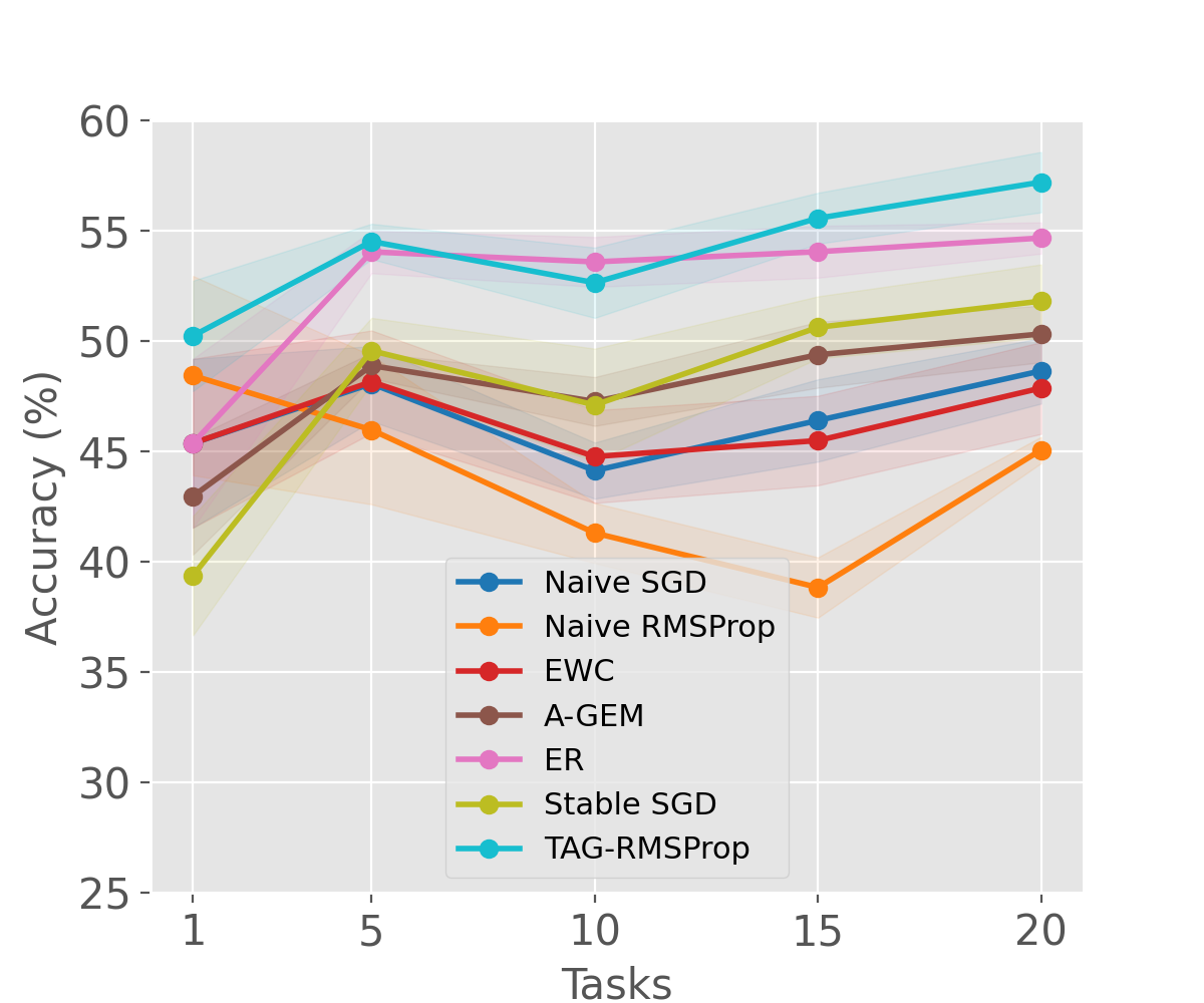
(b) Split-miniImageNet

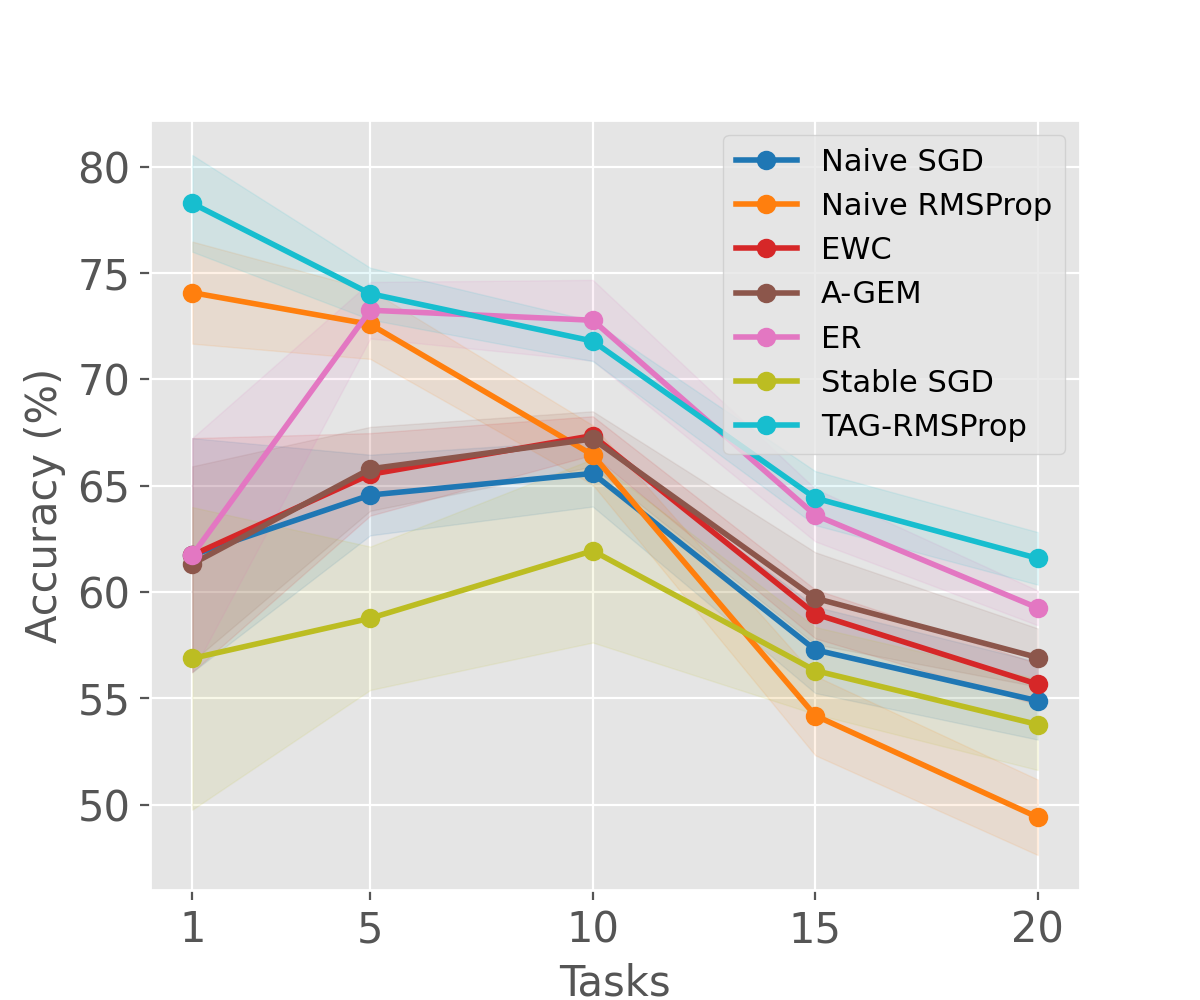
(c) Split-CUB

Figure 3: Evolution of average test Accuracy (%) $A_{t}$ for different existing methods and TAG-RMSProp throughout the stream in Split-CIFAR100, Split-miniImageNet and Split-CUB. All results are averaged across 5 runs and the shaded area represent standard deviation. Performing similar as ER for major part of the stream, TAG-RMSProp always results in the highest final accuracy as compared to other methods with a low standard deviation.

Figure 3 provides a detailed view of the test Accuracy of individual baseline as the model encounters the new tasks throughout the LLL stream in Split-CIFAR100, Split-miniImageNet and Split-CUB. At the starting task $t=1$, TAG-RMSProp beats other baselines because of lower initial learning rates (see Appendix A.2.1) and reflects the performance gain by the RMSProp over SGD optimizer. In all three datasets, the performance of TAG-RMSProp is very similar to ER specially from task $t=5$ to task $t=15$, but ultimately improves as observed at $t=20$. These results show a decent gain in the final test Accuracy by TAG-RMSProp as compared to other baselines. To analyze how the presence of similar tasks help the model to perform better, we also perform the experiment with Rotated MNIST (Lopez-Paz & Ranzato, 2017) dataset, details of which are given in Appendix A.3.2.

4.3 Combined with other baselines

Lastly, we show that the existing baselines can also benefit from our proposed method TAG-RMSProp. We replace the conventional SGD update from EWC, A-GEM and ER, and apply RMSProp update (Eq. 1) and TAG-RMSProp update (Eq. 3) respectively. We use the same task-incremental learning setup as used in the previous sections in terms of architecture and hyper-parameters. We compare the resulting accuracies of the baselines with their RMSProp and TAGed versions in Fig. 4.

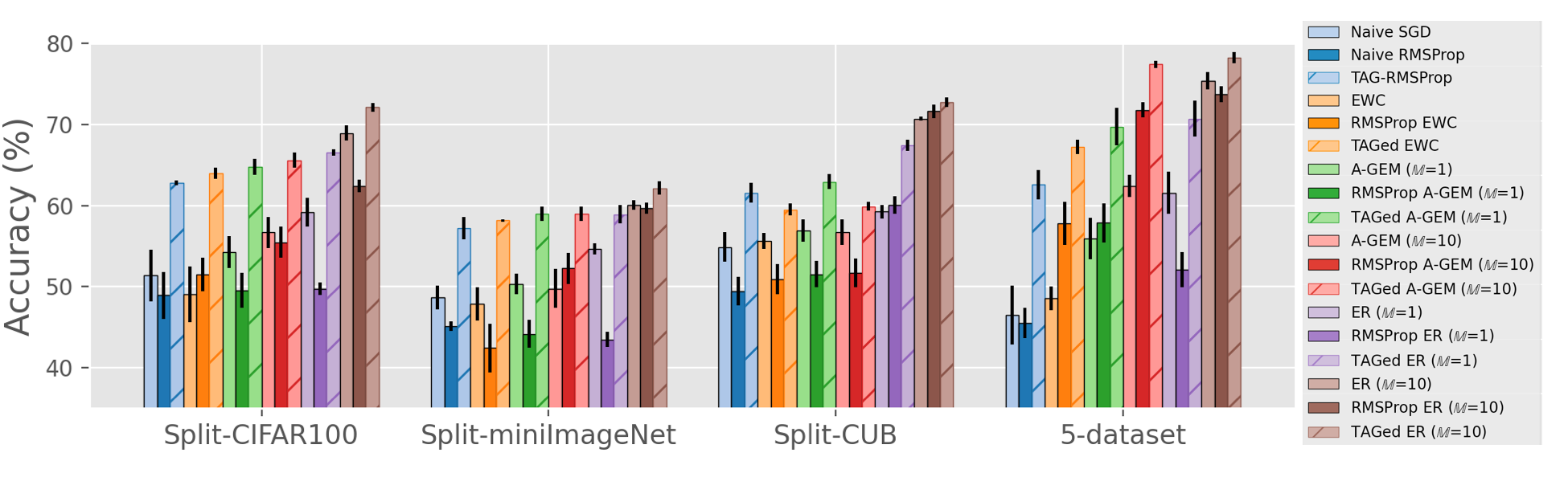
Figure 4: Comparing performance for different existing methods with their RMSProp and TAGed versions on all four datasets in terms of final average test Accuracy (%) along with A-GEM and ER for different samples per class ($\mathbb{M}$) in the episodic memory. The vertical bars with hatches are the performance by TAGed versions of the baselines. All results are averaged across 5 runs. All TAGed versions results in a similar gain in the accuracy over baselines with both SGD and RMSProp update.

For a given dataset, we see that gain in the final accuracy in the TAGed versions is similar for the baselines described in Section 4.2. That is, TAG improves these baselines with SGD update on Split-CIFAR100, Split-miniImageNet, Split-CUB and 5-dataset by at least $8\%$, $4\%$, $4\%$ and $9\%$ respectively. On the other hand, TAG improves the baselines with RMSProp update on the datasets by at least $12\%$, $12\%$, $7\%$ and $9\%$ respectively. The improvement is also significant in A-GEM with bigger episodic memory (i.e., $10$ samples per class or $\mathbb{M}=10$) but we observe relatively smaller improvement (2%) by TAGed ER ($\mathbb{M}=10$) as compared to ER ($\mathbb{M}=10$). These results show that apart from outperforming the baselines independently (with smaller episodic memory in replay-based methods), TAG can also be used as an update rule in the existing research works for improving their performances.

While A-GEM and ER are strong baselines for LLL, we would like to highlight that these replay-based methods are not applicable in settings where storing examples is not an option due to privacy concerns. TAG-RMSProp would be a more appropriate solution in such settings.

5 Conclusion

We propose a new task-aware optimizer for the LLL setting that adapts the learning rate based on the relatedness among tasks. We introduce the task-based accumulated gradients that act as the representation for individual tasks for the same. We conduct experiments on complex datasets to compare TAG-RMSProp with several state-of-the-art methods. Results show that TAG-RMSProp outperforms the existing methods in terms of final accuracy with a commendable margin without storing past examples or using dynamic architectures. We also show that it results in a significant gain in performance when combined with other baselines. To the best of our knowledge, ours is the first work in the LLL literature showing that we can use an adaptive gradient method for LLL and prevent forgetting better than Naive SGD. For future work, as the memory required to store the task-specific accumulated gradients increases linearly with the tasks, reducing memory complexity without compromising the performance can be an interesting direction. This can be achieved by (i) computing correlation using a smaller quantity than the task-based first moments, and (ii) clustering the similar tasks together to reduce the number of task-based second moments (in settings with a soft margin between the tasks). Another possible direction from here can be shifting to a class-incremental scenario where the task identity is not known beforehand and is required to be inferred along the stream.

Appendix A Appendix

In this document, we provide the details and results excluded from the main paper. In A.1, we describe the TAG versions of Adagrad and Adam. The implementation details are described in Section A.2. We also report results obtained by performing additional experiments in Section A.3.

A.1 TAG-optimizers

Similar to RMSProp (in Section 3), with the task-based first moments $M^{(t)}_{n}$, let $W^{(t)}_{n}=\{\alpha_{n}(t,\tau);\tau\in[1,t]\}$ (from Eq. 2) and,

$$W^{(t)}_{n}\textbf{V}^{(t)}_{n} =\begin{cases}V^{(1)}_{n}~{};&t=1\\ \alpha_{n}(t,t)~{}V^{(t)}_{n}+\sum\limits_{\tau=1}^{t-1}\alpha_{n}(t,\tau)~{}V^{(\tau)}_{N}~{};&t>1\end{cases}$$ (4)

We define the TAG versions of Adagrad and Adam as following:

• TAG-Adagrad:

  $$\begin{split}V^{(t)}_{n}&=V^{(t)}_{n-1}+g^{2}_{n}\\ \theta^{(t)}_{n+1}&=\theta^{(t)}_{n}-\frac{\eta}{\sqrt{W^{(t)}_{n}\textbf{V}_{n}+\epsilon}}g_{n}\\ \end{split}$$ (5)

• TAG-Adam:

  $$\begin{split}V^{(t)}_{n}&=\beta_{2}V^{(t)}_{n-1}+(1-\beta_{2})g^{2}_{n}\\ \theta^{(t)}_{n+1}&=\theta^{(t)}_{n}-\frac{\eta\sqrt{1-\beta_{2}^{n}}}{(1-\beta_{1}^{n})\sqrt{W^{(t)}_{n}\textbf{V}_{n}+\epsilon}}M^{(t)}_{n}\\ \end{split}$$ (6)

Both TAG-Adagrad (Eq. 5) and TAG-Adam (Eq. 6) result in a significant gain in Accuracy and prevent Forgetting as observed in Fig. 1(a) and Fig. 1(b) respectively in Section 4.1.

A.2 Implementation details

The summary of the datasets used in the experiments is shown in Table 2 and Table 3.

Table 2: Dataset Statistics

	Input size	Training samples per task	Test samples per task
Split-CIFAR100	$3\times 32\times 32$	$2500$	$500$
Split-miniImageNet	$3\times 84\times 84$	$2400$	$600$
Split-CUB	$3\times 224\times 224$	$300$	$290$

In 5-dataset, we convert all the monochromatic images to RGB format depending on the task dataset. All images are then resized to $3\times 32\times 32$. The overall training and test data statistics of 5-dataset are described in Table 3.

Table 3: 5-dataset statistics.

	Training samples	Test samples
CIFAR-10	$50000$	$10000$
MNIST	$60000$	$10000$
SVHN	$73257$	$26032$
notMNIST	$16853$	$1873$
Fashion-MNIST	$60000$	$10000$

Details about the metrics used for evaluating the model:

• Accuracy (Lopez-Paz & Ranzato, 2017): If $a_{t,\tau}$ is the accuracy on the test set of task $\tau$ when the current task is $t$, it is defined as, $A_{t}=\frac{1}{t}\sum\limits_{\tau=1}^{t}a_{t,\tau}$.

• Forgetting (Chaudhry et al., 2018a): It is the average forgetting that occurs after the model is trained on all tasks. If the latest task is $t$ and is defined as, $F_{t}=\frac{1}{t-1}\sum\limits_{\tau=1}^{t-1}\max_{t^{\prime}\in\{1,...,t-1\}}(a_{t^{\prime},\tau}-a_{t,\tau})$.

• Learning Accuracy (LA) (Riemer et al., 2018): It is the measure of learning capability when the model sees a new task. For the current task $t$, it is defined as, $L_{t}=\frac{1}{t}\sum\limits_{\tau=1}^{t}a_{\tau,\tau}$.

We implement the following baselines to compare with our proposed method:

• EWC: Our implementation of EWC is based on the original paper (Kirkpatrick et al., 2017).

• A-GEM: We implemented A-GEM based on the the official implementation provided by (Chaudhry et al., 2018b).

• ER (Chaudhry et al., 2019): Our implementation is based on the one provided by (Aljundi et al., 2019) with reservoir sampling except that the sampled batch does not contain examples from the current task.

• Stable SGD (Mirzadeh et al., 2020): We obtain the best hyper-parameter set by performing grid-search over different combinations of the learning rate, learning rate decay, and dropout (see Appendix A.2.1).

We provide our code as supplementary material that contains the scripts for reproducing the results from experiments described in this paper. In the code folder, we include readme.md file that contains the overall code structure, procedure for installing the required packages, links to download the datasets and steps to execute the scripts. All experiments were executed on an NVIDIA GTX 1080Ti machine with 11 GB GPU memory.

A.2.1 Hyper-parameter details

In this section, we report the grid search details for finding the best set of hyper-parameters for all datasets and baselines. We train the model with $90\%$ of the training set and choose the best hyper-parameters based on the highest accuracy on the validation set which consists of remaining $10\%$ for the training set. For existing baselines, we perform the grid search either suggested by the original papers or by Farajtabar et al. (2020). For all TAG-optimizers, $\beta_{1}$ is set to $0.9$. For TAG-RMSProp and TAG-Adagrad, $\beta_{2}$ is set to $0.99$ and for TAG-Adam it is $0.999$. In all the experiments, the mini-batch size is fixed to $10$ for Split-CIFAR100, Split-miniImageNet, Split-CUB similar to (Chaudhry et al., 2019; Mirzadeh et al., 2020). We set mini-batch size to $64$ for 5-dataset following (Serra et al., 2018). This is because we wanted to highlight the role of learning rate and to show how TAG-RMSProp improves the performance while the other hyper-parameters (including batch-size) were fixed.

• Naive SGD

  • Learning rate: [0.1 (Split-CIFAR100, 5-dataset), 0.05 (Split-miniImageNet), 0.01(Split-CUB), 0.001]

• Naive Adagrad

  • Learning rate: [0.01, 0.005 (Split-CIFAR100, Split-miniImageNet, 5-dataset), 0.001, 0.0005 (Split-CUB), 0.0001]

• Naive RMSProp

  • Learning rate: [0.01, 0.005 (Split-CIFAR100), 0.001 (Split-miniImageNet, 5-dataset), 0.0005, 0.0001 (Split-CUB), 0.00005, 0.00001]

• Naive Adam

  • Learning rate: [0.01, 0.005 (Split-CIFAR100), 0.001 (Split-miniImageNet, 5-dataset), 0.0005, 0.0001 (Split-CUB)]

• TAG-Adagrad

  • Learning rate: [0.005 (Split-CIFAR100, 5-dataset), 0.001 (Split-miniImageNet), 0.0005 (Split-CUB), 0.00025, 0.0001]

  • $b$: [1, 3, 5 (Split-CIFAR100, Split-miniImageNet, Split-CUB), 7 (5-dataset)]

• TAG-RMSProp

  • Learning rate: [0.005, 0.001, 0.0005 (5-dataset), 0.00025 (Split-CIFAR100), 0.0001 (Split-miniImageNet), 0.00005, 0.000025 (Split-CUB), 0.00001]

  • $b$: [1, 3, 5 (Split-CIFAR100, Split-miniImageNet, Split-CUB), 7 (5-dataset)]

• TAG-Adam

  • Learning rate: [0.005, 0.001 (5-dataset), 0.0005 (Split-CIFAR100), 0.00025 (Split-miniImageNet), 0.0001 (Split-CUB)]

  • $b$: [1, 3, 5 (Split-CIFAR100, Split-miniImageNet, Split-CUB), 7 (5-dataset)]

• EWC

  • Learning rate: [0.1 (Split-CIFAR100, 5-dataset), 0.05 (Split-miniImageNet), 0.01(Split-CUB), 0.001]

  • $\lambda$ (regularization): [1 (Split-CIFAR100, Split-miniImageNet, Split-CUB), 10, 100 (5-dataset)]

• A-GEM

  • Learning rate: [0.1 (Split-CIFAR100, Split-miniImageNet, 5-dataset), 0.05, 0.01(Split-CUB), 0.001]

• ER

  • Learning rate: [0.1 (Split-CIFAR100, 5-dataset), 0.05 (Split-miniImageNet), 0.01(Split-CUB), 0.001]

• Stable SGD

  • Initial learning rate: [0.1 (Split-CIFAR100, Split-miniImageNet, 5-dataset), 0.05 (Split-CUB), 0.01]

  • Learning rate decay: [0.9 (Split-CIFAR100, Split-miniImageNet, Split-CUB), 0.8, 0.7 (5-dataset)]

  • Dropout: [0.0 (Split-miniImageNet, Split-CUB, 5-dataset), 0.1 (Split-CIFAR100), 0.25, 0.5]

In case of TAG-RMSProp, we empirically found that the best performance of the all three benchmarks with $20$ tasks occurred when hyper-parameter $b=5$ and for 5-dataset, $b=7$. We also found that a lower value of Learning rate in TAG-RMSProp results in a better performance. These empirical observations can reduce the search space for hyperparameter setup by a huge amount when applying TAG-RMSProp on a LLL setup.

For the experiments in Section 4.3 that require a hybrid version of these methods, we use the same hyperparameters from above except for TAGed ER in Split-CIFAR100 (Learning rate = 0.0005) and Split-CUB (Learning rate = 0.0001). We choose the learning rates of TAG-RMSProp and Naive-RMSProp over EWC, A-GEM and ER.

A.3 Additional Experiments

In this section, we describe the additional experiments and analysis done in this work.

A.3.1 Backward Transfer Metric

While we show the occurrence of knowledge transfer in Fig. 2, we can quantify the Backward Transfer (BWT) (Chaudhry et al., 2019) by computing the difference between the final Accuracy and LA. i.e.,
$\textbf{BWT}=\frac{1}{t-1}\sum_{\tau=1}^{t-1}a_{t,\tau}-a_{\tau,\tau}$. We report the BWT results for all datasets and baselines in Table 4.

While TAG-RMSProp outperforms the other baselines in terms of BWT for Split-miniImageNet, it is overall the second-best method for Split-CIFAR100 and 5-dataset. In case of Split-CUB, even if TAG-RMSProp achieves the highest Accuracy, it results in a lower BWT because of a significantly higher LA as compared to the other baselines (see Table 1).

Table 4: Comparing performance in terms of final average test Accuracy (%) (higher is better) and BWT (higher is better) with the standard deviation values for different existing methods with TAG-RMSProp for all four datasets. All metrics are averaged across 5 runs.

Methods	Split-CIFAR100		Split-miniImageNet
	Accuracy (%)	BWT (%)	Accuracy (%)	BWT (%)
Naive SGD	$51.36~{}(\pm 3.21)$	$-17.1~{}(\pm 2.64)$	$48.19~{}(\pm 0.79)$	$-13.83~{}(\pm 1.97)$
Naive RMSProp	$48.91~{}(\pm 2.88)$	$-18.37~{}(\pm 2.71)$	$45.06~{}(\pm 0.6)$	$-19.32~{}(\pm 1.39)$
EWC	$49.06~{}(\pm 3.44)$	$-17.76~{}(\pm 3.35)$	$47.87~{}(\pm 2.08)$	$-13.79~{}(\pm 2.26)$
A-GEM	$54.25~{}(\pm 2.0)$	$-14.73~{}(\pm 2.48)$	$50.32~{}(\pm 1.29)$	$-10.69~{}(\pm 1.57)$
ER	$59.14~{}(\pm 1.77)$	$-11.22~{}(\pm 2.19)$	$54.67~{}(\pm 0.71)$	$-9.39~{}(\pm 0.64)$
Stable SGD	$57.04~{}(\pm 1.07)$	$-7.59~{}(\pm 0.36)$	$51.81~{}(\pm 1.66)$	$-8.18~{}(\pm 1.18)$
TAG-RMSProp (Ours)	$\textbf{62.79}~{}(\pm 0.29)$	$-9.27~{}(\pm 1.16)$	$\textbf{57.2}~{}(\pm 1.37)$	$-5.52~{}(\pm 1.71)$

Methods	Split-CUB		5-dataset
	Accuracy (%)	BWT (%)	Accuracy (%)	BWT (%)
Naive SGD	$54.88~{}(\pm 1.83)$	$-11.09~{}(\pm 1.43)$	$46.48~{}(\pm 3.62)$	$-38.06~{}(\pm 3.69)$
Naive RMSProp	$49.4~{}(\pm 1.77)$	$-22.36~{}(\pm 0.95)$	$45.49~{}(\pm 1.89)$	$-40.09~{}(\pm 2.6)$
EWC	$55.66~{}(\pm 0.97)$	$-10.7~{}(\pm 0.39)$	$48.58~{}(\pm 1.47)$	$-30.98~{}(\pm 3.34)$
A-GEM	$56.91~{}(\pm 1.37)$	$-8.69~{}(\pm 0.93)$	$55.9~{}(\pm 2.58)$	$-26.71~{}(\pm 3.6)$
ER	$59.25~{}(\pm 0.82)$	$-6.93~{}(\pm 0.92)$	$61.58~{}(\pm 2.65)$	$-22.72~{}(\pm 3.08)$
Stable SGD	$53.76~{}(\pm 2.14)$	$-8.39~{}(\pm 1.26)$	$46.51~{}(\pm 2.75)$	$-36.79~{}(\pm 2.19)$
TAG-RMSProp (Ours)	$\textbf{61.58}~{}(\pm 1.24)$	$-9.99~{}(\pm 1.62)$	$\textbf{62.59}~{}(\pm 1.82)$	$-23.49~{}(\pm 1.73)$

A.3.2 Comparing with other baselines on Rotated-MNIST and 5-dataset

We evaluate the performance of TAG-RMSProp on Rotated MNIST and 5-dataset and in terms of average test Accuracy on each task in the stream.

Here, Rotated MNIST (Lopez-Paz & Ranzato, 2017) is a version of MNIST dataset (LeCun, 1998) where the images in a task are basically MNIST images with some fixed degrees of rotation. In our experiment, we consider $10$ tasks where we incrementally rotate the images by $30^{\circ}$ for each task.

The goal of this experiment to answer two questions: (i) Is the proposed way to find similar tasks by computing correlation between task-based first moments valid? (ii) Can the presence of similar tasks in the stream help model to perform better?

We plot the Accuracy for Naive SGD, ER and TAG-RMSProp in Figure 5. Best performance of Naive SGD and ER was observed with learning rates $0.1$. For TAG-RMSProp, we found the setting with $learningrate=0.00025$ and $b=5$ results in the best final Accuracy. Details of 5-dataset is given in Appendix A.2.

In Figure 5(a), we observe that TAG-RMSProp not only outperforms ER but there is a significant gain in Accuracy at $t=7$ (i.e., images with $180^{\circ}$ rotation). Since there are several digits that could look exactly same even with $180^{\circ}$ rotation, TAG recognizes the similarity between $t=7$ and $t=1$ and is able to transfer the gained knowledge to result it increase in the Accuracy. This observation answers the above two questions since similar tasks in Rotated MNIST are recognized by TAG and also help in improving the performance. As observed in Figure 5(b), although TAG-RMSProp is outperformed by ER from task $t=2$ (MNIST) to $t=4$ (notMNIST) for 5-dataset, it results in the highest final Accuracy as compared to other methods. Moreover, the increase in Accuracy from $t=2$ (MNIST) to $t=3$ (SVHN) also shows the positive transfer exhibited by TAG as compared to ER.

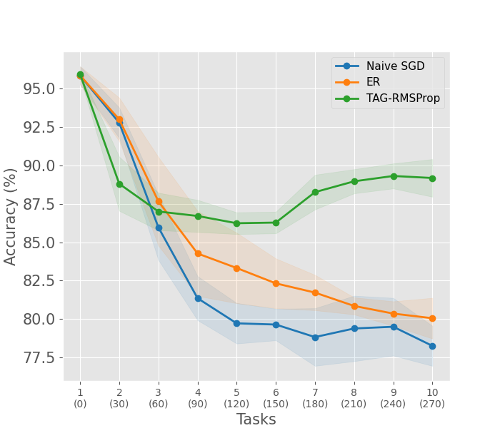
(a) Rotated MNIST

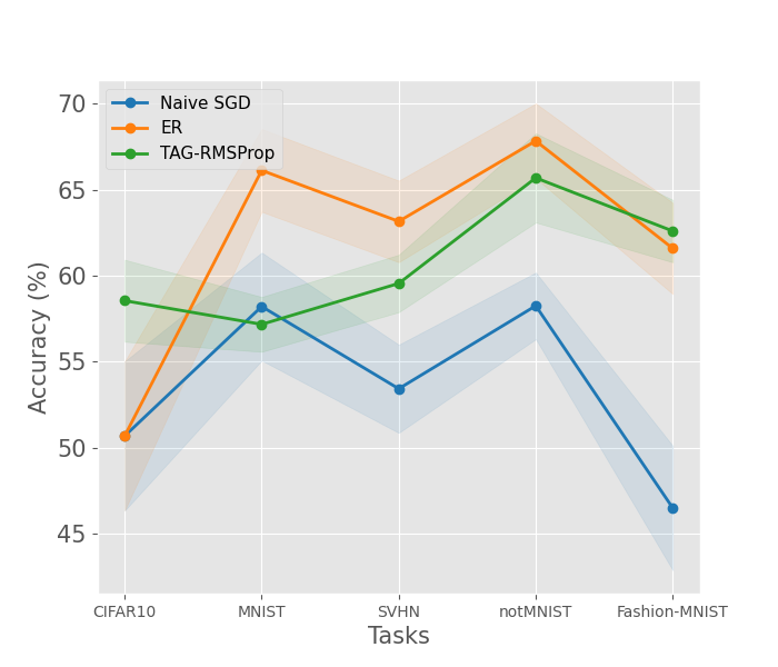
(b) 5-dataset

Figure 5: Evolution of average test Accuracy (%) $A_{t}$ for different existing methods and TAG-RMSProp throughout the stream in Rotated MNIST and 5-dataset. All results are averaged across 5 runs and the shaded area represent standard deviation.

A.3.3 Evolution of $\alpha(t,\tau)$ and Test Accuracy $a_{t,\tau}$

Next, we continue the analysis done in Section 4.1 for Split-CIFAR100 (in Fig. 6), Split-miniImageNet (in Fig. 7), Split-CUB (in Fig. 8) for the first $9$ tasks and 5-dataset (in Fig. 9) for first $3$ tasks. In Split-CIFAR100 and Split-miniImageNet, the model with Naive RMSProp tends to forget the task $t$ by significant amount as soon as it receives the new tasks. On the other hand, TAG-RMSProp prevents catastrophic forgetting and hence results in a higher accuracy throughout the stream. We can observe that for Split-CIFAR100 and Split-miniImageNet, $\alpha(\tau+1,\tau)$ (where $\tau\in[1,9]$) generally have a higher rank in the set $\{\alpha(t,\tau^{\prime});\tau^{\prime}\in[1,t]\}$. This is because TAG-RMSProp also recognizes an immediate change in the directions when the model receives a new task (from $M^{(t-1)}_{N}$ to $M^{(t)}_{n}$). A similar observation is made in case of Split-CUB but the visible gain in the accuracy by TAG-RMSProp does not occur instantly. Apart from that, we observe that the lower and higher rank of $\alpha(t,\tau)$ results in backward transfer and prevents catastrophic forgetting respectively in the stream. Overall, in all datasets, we arrive at the same conclusion obtained in Section 4.1.

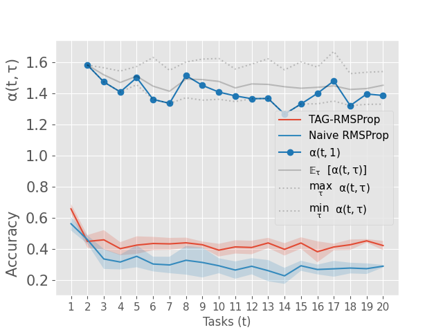
(a) $\tau=1$

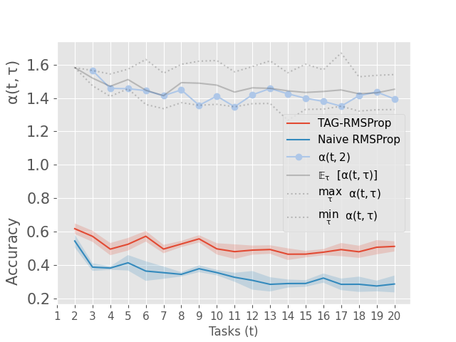
(b) $\tau=2$

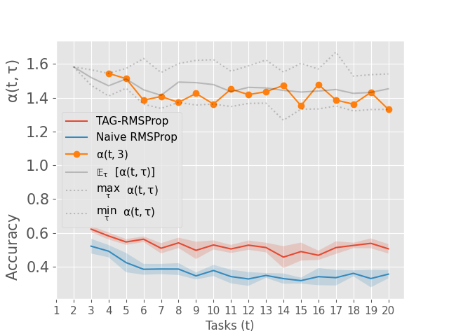
(c) $\tau=3$

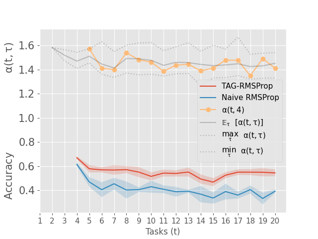
(d) $\tau=4$

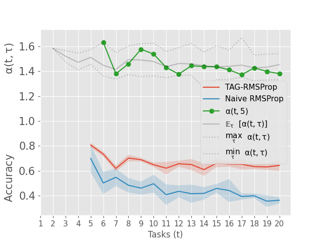
(e) $\tau=5$

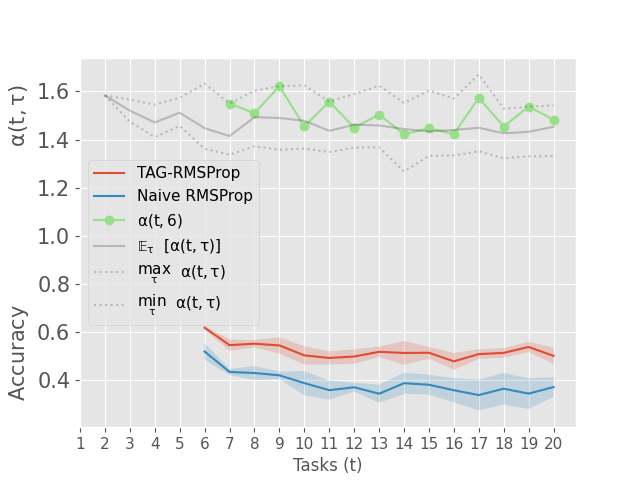
(f) $\tau=6$

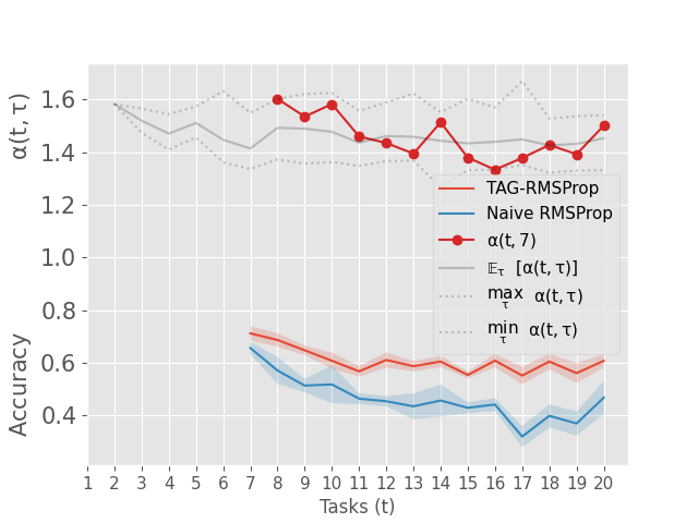
(g) $\tau=7$

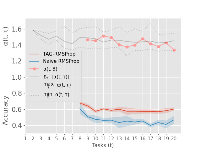
(h) $\tau=8$

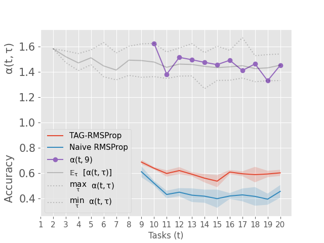
(i) $\tau=9$

Figure 6: Evolution of $\alpha(t,\tau)$ and test accuracy $a_{t,\tau}$ where $\tau\in[1,9]$ along the stream of $20$ tasks in the Split-CIFAR100 dataset. The grey-coloured lines are $\max_{\tau^{\prime}}\alpha_{n}(t,\tau^{\prime})$ (top, dashed line), $\mathbb{E}_{\tau^{\prime}}[\alpha(t,\tau^{\prime})]$ (middle, solid line) and $\min_{\tau^{\prime}}\alpha(t,\tau^{\prime})$ (bottom, dashed line) that indicate the range of $\alpha(t,\tau^{\prime})$.

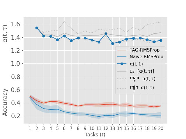
(a) $\tau=1$

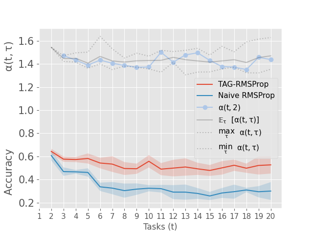
(b) $\tau=2$

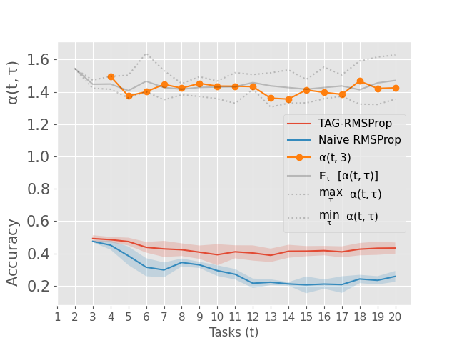
(c) $\tau=3$

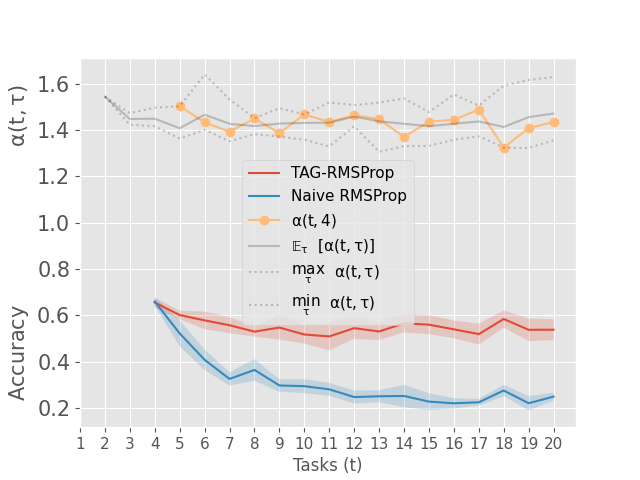
(d) $\tau=4$

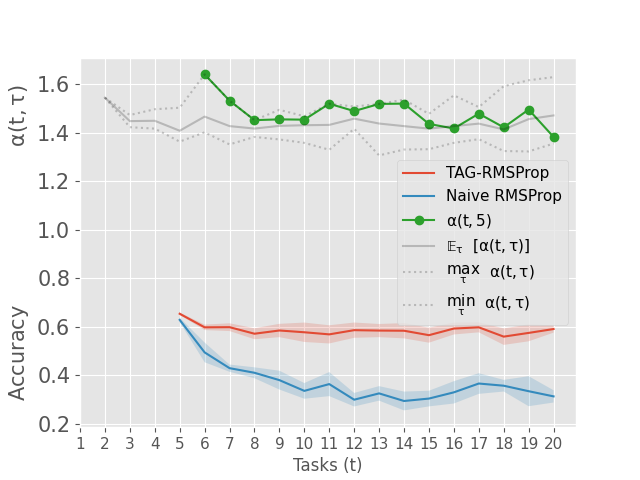
(e) $\tau=5$

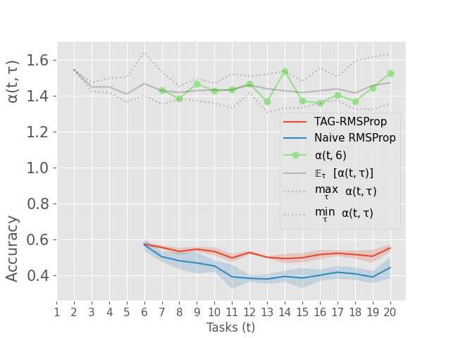
(f) $\tau=6$

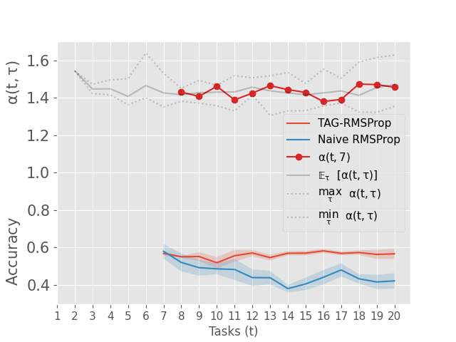
(g) $\tau=7$

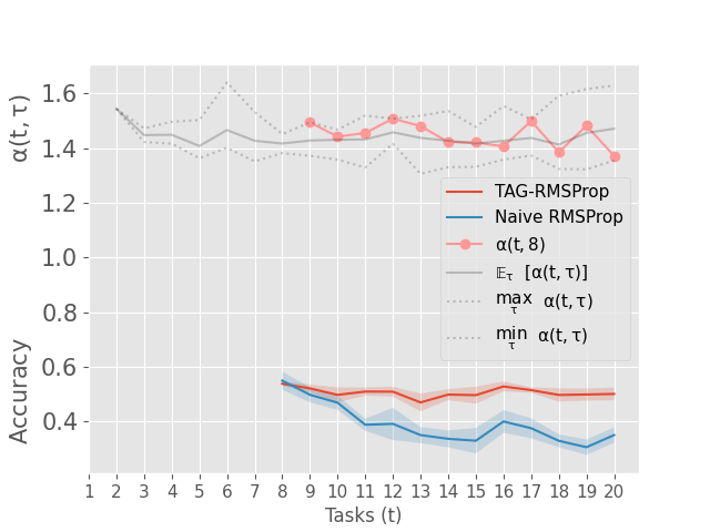
(h) $\tau=8$

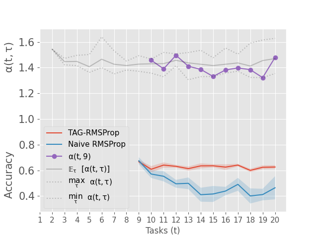
(i) $\tau=9$

Figure 7: Evolution of $\alpha(t,\tau)$ and test accuracy $a_{t,\tau}$ where $\tau\in[1,9]$ along the stream of $20$ tasks in the Split-miniImageNet dataset. The grey-coloured lines are $\max_{\tau^{\prime}}\alpha_{n}(t,\tau^{\prime})$ (top, dashed line), $\mathbb{E}_{\tau^{\prime}}[\alpha(t,\tau^{\prime})]$ (middle, solid line) and $\min_{\tau^{\prime}}\alpha(t,\tau^{\prime})$ (bottom, dashed line) that indicate the range of $\alpha(t,\tau^{\prime})$.

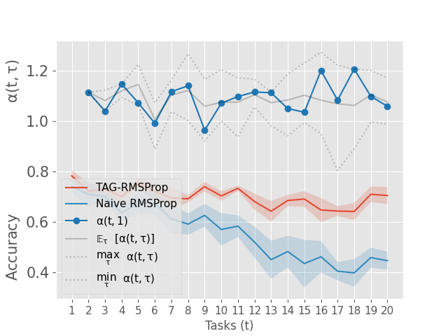
(a) $\tau=1$

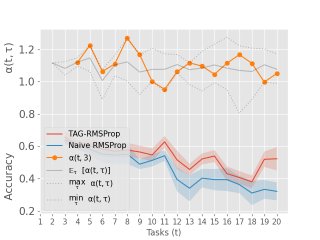
(b) $\tau=3$

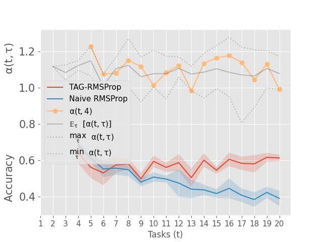
(c) $\tau=4$

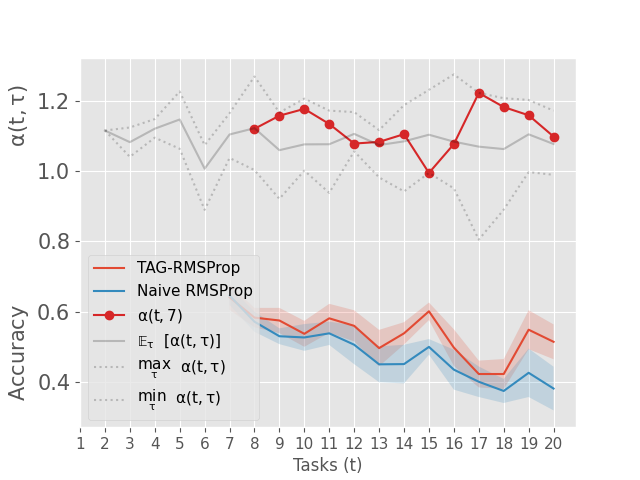
(d) $\tau=7$

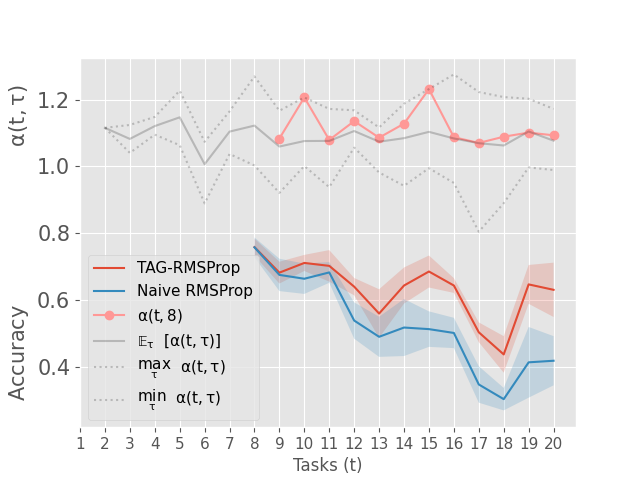
(e) $\tau=8$

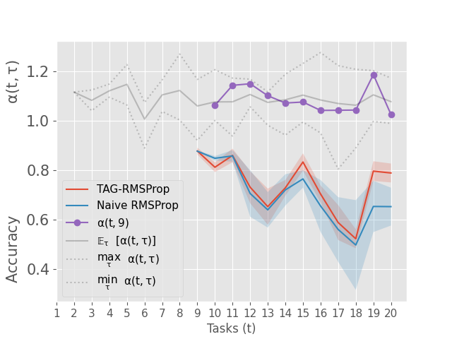
(f) $\tau=9$

Figure 8: Evolution of $\alpha(t,\tau)$ and test accuracy $a_{t,\tau}$ where $\tau\in\{1,3,4,7,8,9\}$ along the stream of $20$ tasks in the Split-CUB dataset. The grey-coloured lines are $\max_{\tau^{\prime}}\alpha_{n}(t,\tau^{\prime})$ (top, dashed line), $\mathbb{E}_{\tau^{\prime}}[\alpha(t,\tau^{\prime})]$ (middle, solid line) and $\min_{\tau^{\prime}}\alpha(t,\tau^{\prime})$ (bottom, dashed line) that indicate the range of $\alpha(t,\tau^{\prime})$.

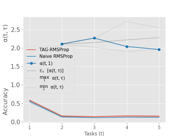
(a) $\tau=1$

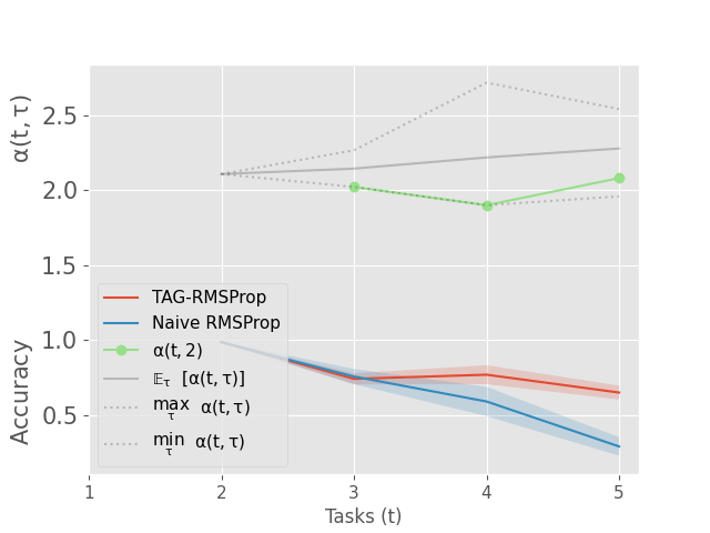
(b) $\tau=2$

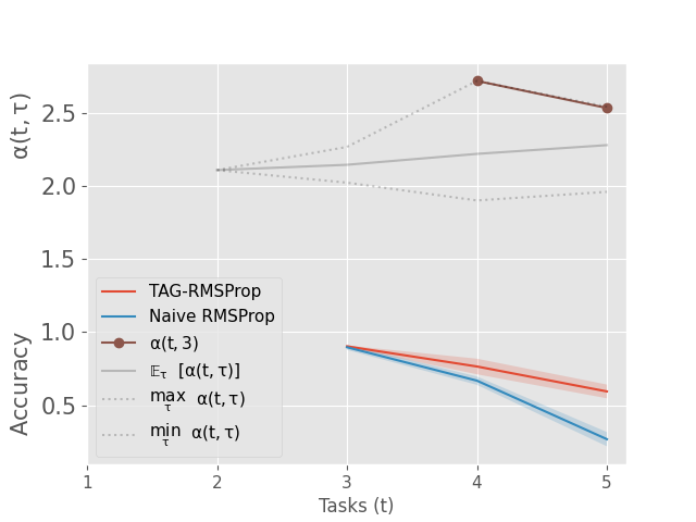
(c) $\tau=3$

Figure 9: Evolution of $\alpha(t,\tau)$ and test accuracy $a_{t,\tau}$ where $\tau\in\{1,2,3\}$ along the stream of $5$ tasks in the 5-dataset dataset. The grey-coloured lines are $\max_{\tau^{\prime}}\alpha_{n}(t,\tau^{\prime})$ (top, dashed line), $\mathbb{E}_{\tau^{\prime}}[\alpha(t,\tau^{\prime})]$ (middle, solid line) and $\min_{\tau^{\prime}}\alpha(t,\tau^{\prime})$ (bottom, dashed line) that indicate the range of $\alpha(t,\tau^{\prime})$.

A.3.4 Multiple-pass per Task

In this section, we report the performance of TAG-RMSProp and all other baselines discussed in Section 4.2 for 5 epochs per task in Table 5. Hyper-parameters for this experiment are kept the same as the single-pass per task setting. TAG-RMSProp results in high average Accuracy in all the datasets. We also observe less amount of Forgetting in TAG-RMSProp as compared to other baselines. In terms of Learning Accuracy, TAG-RMSProp is outperformed by the other baselines in Split-CIFAR100, Split-miniImageNet and 5-dataset but performs better in Split-CUB.

Table 5: Comparing performance in terms of Final average test Accuracy (%) (higher is better), Forgetting (lower is better) and Learning Accuracy (LA (%)) (higher is better) with the standard deviation values for different existing methods with TAG-RMSProp running for 5 epochs per task for all four datasets (see Section 4). All metrics are averaged across 5 runs. *MTL assumes that the dataset from all tasks are always available during training, hence it is a different setting and its accuracy acts as an upper bound.

Methods	Split-CIFAR100			Split-miniImageNet
	Accuracy (%)	Forgetting	LA (%)	Accuracy (%)	Forgetting	LA (%)
Naive SGD	$52.26~{}(\pm 0.65)$	$0.28~{}(\pm 0.01)$	$78.45~{}(\pm 0.41)$	$46.9~{}(\pm 1.18)$	$0.25~{}(\pm 0.02)$	$70.82~{}(\pm 0.6)$
Naive RMSProp	$46.12~{}(\pm 2.33)$	$0.32~{}(\pm 0.02)$	$76.29~{}(\pm 0.53)$	$41.07~{}(\pm 0.66)$	$0.32~{}(\pm 0.01)$	$71.43~{}(\pm 0.42)$
EWC	$51.7~{}(\pm 1.71)$	$0.27~{}(\pm 0.02)$	$77.72~{}(\pm 0.84)$	$48.17~{}(\pm 0.81)$	$0.25~{}(\pm 0.01)$	$71.87~{}(\pm 0.26)$
A-GEM	$54.24~{}(\pm 1.14)$	$0.25~{}(\pm 0.01)$	$78.38~{}(\pm 0.39)$	$49.08~{}(\pm 0.52)$	$0.23~{}(\pm 0.01)$	$70.49~{}(\pm 0.4)$
ER	$60.03~{}(\pm 0.96)$	$0.19~{}(\pm 0.01)$	$78.15~{}(\pm 0.7)$	$54.01~{}(\pm 0.56)$	$0.19~{}(\pm 0.01)$	$71.77~{}(\pm 0.58)$
Stable SGD	$58.92~{}(\pm 0.73)$	$0.19~{}(\pm 0.01)$	$76.91~{}(\pm 0.72)$	$51.23~{}(\pm 0.88)$	$0.22~{}(\pm 0.01)$	$71.77~{}(\pm 0.56)$
TAG-RMSProp (Ours)	$60.64~{}(\pm 1.38)$	$0.17~{}(\pm 0.01)$	$77.12~{}(\pm 0.76)$	$\textbf{58.0}~{}(\pm 1.11)$	$0.11~{}(\pm 0.02)$	$68.14~{}(\pm 0.38)$
MTL*	$67.7~{}(\pm 0.58)$	-	-	$66.14~{}(\pm 1.0)$	-	-

Methods	Split-CUB			5-dataset
	Accuracy (%)	Forgetting	LA (%)	Accuracy (%)	Forgetting	LA (%)
Naive SGD	$59.87~{}(\pm 1.48)$	$0.21~{}(\pm 0.02)$	$79.77~{}(\pm 0.44)$	$49.95~{}(\pm 2.42)$	$0.51~{}(\pm 0.04)$	$90.86~{}(\pm 0.63)$
Naive RMSProp	$35.87~{}(\pm 1.14)$	$0.46~{}(\pm 0.01)$	$79.59~{}(\pm 0.3)$	$50.47~{}(\pm 0.99)$	$0.51~{}(\pm 0.01)$	$90.89~{}(\pm 0.44)$
EWC	$59.73~{}(\pm 2.4)$	$0.21~{}(\pm 0.02)$	$79.8~{}(\pm 0.58)$	$52.51~{}(\pm 7.34)$	$0.43~{}(\pm 0.09)$	$86.8~{}(\pm 2.52)$
A-GEM	$62.65~{}(\pm 1.61)$	$0.17~{}(\pm 0.02)$	$79.1~{}(\pm 0.4)$	$62.48~{}(\pm 3.16)$	$0.35~{}(\pm 0.04)$	$90.53~{}(\pm 0.73)$
ER	$66.06~{}(\pm 1.28)$	$0.14~{}(\pm 0.02)$	$78.79~{}(\pm 0.55)$	$62.84~{}(\pm 1.58)$	$0.35~{}(\pm 0.02)$	$90.52~{}(\pm 0.69)$
Stable SGD	$58.75~{}(\pm 0.96)$	$0.19~{}(\pm 0.01)$	$76.6~{}(\pm 0.64)$	$51.95~{}(\pm 3.83)$	$0.48~{}(\pm 0.05)$	$90.41~{}(\pm 0.29)$
TAG-RMSProp (Ours)	$\textbf{68.0}~{}(\pm 1.01)$	$0.13~{}(\pm 0.01)$	$80.15~{}(\pm 0.22)$	$61.13~{}(\pm 3.05)$	$0.36~{}(\pm 0.04)$	$89.9~{}(\pm 0.33)$
MTL*	$71.65~{}(\pm 0.76)$	-	-	$70.0~{}(\pm 4.44)$	-	-

A.3.5 Bigger Memory size in replay-based methods

We also compare the performance of A-GEM and ER with a larger number of samples per class ($\mathbb{M}$) in the episodic memory for all four datasets in Table 6. With $\mathbb{M}=10$, total episodic memory size for Split-CIFAR100, Split-miniImageNet, Split-CUB and 5-dataset becomes $1000$, $1000$, $2000$ and $500$ respectively. We observe ER results in a significant gain in the performance as the episodic memory size increases. But TAG-RMSProp is able to outperform A-GEM in Split-CIFAR100, Split-miniImageNet and Split-CUB with a large margin even when $\mathbb{M}$ is set to $10$.

Table 6: Comparing performance in terms of Final average test Accuracy (%) (higher is better), Forgetting (lower is better) and Learning Accuracy (LA (%)) (higher is better) with the standard deviation values for A-GEM and ER for different number of samples per class ($\mathbb{M}$) in the episodic memory with TAG-RMSProp for all four datasets (see Section 4). All metrics are averaged across 5 runs. Overall, ER with bigger memory outperforms all other methods in terms of Accuracy.

Methods	Split-CIFAR100			Split-miniImageNet
	Accuracy (%)	Forgetting	LA (%)	Accuracy (%)	Forgetting	LA (%)
A-GEM ($\mathbb{M}=1$)	$54.25~{}(\pm 2.0)$	$0.16~{}(\pm 0.03)$	$68.98~{}(\pm 1.19)$	$50.32~{}(\pm 1.29)$	$0.11~{}(\pm 0.02)$	$61.02~{}(\pm 0.64)$
A-GEM ($\mathbb{M}=5$)	$55.74~{}(\pm 1.14)$	$0.14~{}(\pm 0.01)$	$68.97~{}(\pm 0.56)$	$49.52~{}(\pm 2.02)$	$0.12~{}(\pm 0.02)$	$60.49~{}(\pm 0.78)$
A-GEM ($\mathbb{M}=10$)	$56.68~{}(\pm 1.92)$	$0.13~{}(\pm 0.02)$	$68.72~{}(\pm 0.96)$	$49.77~{}(\pm 2.41)$	$0.12~{}(\pm 0.02)$	$60.6~{}(\pm 0.66)$
ER ($\mathbb{M}=1$)	$59.14~{}(\pm 1.77)$	$0.12~{}(\pm 0.02)$	$70.36~{}(\pm 1.23)$	$52.76~{}(\pm 1.53)$	$0.1~{}(\pm 0.01)$	$61.7~{}(\pm 0.74)$
ER ($\mathbb{M}=5$)	$65.74~{}(\pm 1.47)$	$0.07~{}(\pm 0.01)$	$70.91~{}(\pm 1.13)$	$58.49~{}(\pm 1.21)$	$0.05~{}(\pm 0.01)$	$62.24~{}(\pm 0.85)$
ER ($\mathbb{M}=10$)	$\textbf{68.94}~{}(\pm 0.93)$	$0.05~{}(\pm 0.01)$	$71.26~{}(\pm 1.01)$	$\textbf{60.06}~{}(\pm 0.63)$	$0.04~{}(\pm 0.01)$	$62.21~{}(\pm 1.24)$
TAG-RMSProp (Ours)	$62.79~{}(\pm 0.29)$	$0.1~{}(\pm 0.01)$	$72.06~{}(\pm 1.01)$	$57.2~{}(\pm 1.37)$	$0.06~{}(\pm 0.02)$	$62.73~{}(\pm 0.61)$

Methods	Split-CUB			5-dataset
	Accuracy (%)	Forgetting	LA (%)	Accuracy (%)	Forgetting	LA (%)
A-GEM ($\mathbb{M}=1$)	$56.91~{}(\pm 1.37)$	$0.1~{}(\pm 0.01)$	$65.6~{}(\pm 0.73)$	$55.9~{}(\pm 2.58)$	$0.34~{}(\pm 0.04)$	$82.61~{}(\pm 2.13)$
A-GEM ($\mathbb{M}=5$)	$56.4~{}(\pm 1.5)$	$0.1~{}(\pm 0.01)$	$65.63~{}(\pm 0.64)$	$61.39~{}(\pm 1.0)$	$0.28~{}(\pm 0.01)$	$83.48~{}(\pm 1.05)$
A-GEM ($\mathbb{M}=10$)	$56.71~{}(\pm 1.6)$	$0.1~{}(\pm 0.01)$	$65.73~{}(\pm 0.9)$	$62.43~{}(\pm 1.38)$	$0.26~{}(\pm 0.03)$	$83.38~{}(\pm 1.79)$
ER ($\mathbb{M}=1$)	$59.25~{}(\pm 0.82)$	$0.1~{}(\pm 0.01)$	$66.17~{}(\pm 0.42)$	$61.58~{}(\pm 2.65)$	$0.28~{}(\pm 0.04)$	$84.31~{}(\pm 1.08)$
ER ($\mathbb{M}=5$)	$68.89~{}(\pm 0.31)$	$0.04~{}(\pm 0.0)$	$66.76~{}(\pm 0.73)$	$71.56~{}(\pm 1.54)$	$0.16~{}(\pm 0.02)$	$84.34~{}(\pm 1.46)$
ER ($\mathbb{M}=10$)	$\textbf{70.73}~{}(\pm 0.23)$	$0.03~{}(\pm 0.01)$	$66.83~{}(\pm 0.86)$	$\textbf{75.44}~{}(\pm 1.07)$	$0.12~{}(\pm 0.02)$	$84.62~{}(\pm 0.89)$
TAG-RMSProp (Ours)	$61.58~{}(\pm 1.24)$	$0.11~{}(\pm 0.01)$	$71.56~{}(\pm 0.74)$	$62.59~{}(\pm 1.82)$	$0.3~{}(\pm 0.02)$	$86.08~{}(\pm 0.55)$

A.3.6 Ablation studies

In the following experiments, we perform ablation studies over TAG-RMSProp.

• Instead of Eq. 2 in TAG-RMSProp, we define TAG-1 where $\alpha_{n}(t,\tau)=1$ i.e., equal importance is given to all task based second moments.

• Similarly, we define TAG-age by replacing Eq. 2 with $\alpha_{n}(t,\tau)=t-\tau+1$ i.e., giving importance to the past tasks based on their age.

• There can be different ways to approximate the gradient directions such as averaging the gradients or storing the gradients for each task etc. Therefore, we define a variant TAG-G, where we store first $\mathbb{B}$ gradients obtained for each task instead of maintaining task-based first moments. When the model sees a new task $t$, we then obtain the $\alpha_{n}(t,\tau)$ by computing cosine similarity between these stored gradients.

We implement TAG-1, TAG-age and TAG-G in our code and run experiments on Split-CIFAR100, Split-miniImageNet, Split-CUB and 5-dataset. For TAG-G, we run it for different values of $\mathbb{B}$. All results shown is Table 7 are averaged across $5$ runs.

Table 7: Comparing performance in terms of Final average test Accuracy (%) (higher is better), Forgetting (lower is better) and Learning Accuracy (LA (%)) (higher is better) with the standard deviation values for different variants of TAG-RMSProp (see Appendix A.3.6) for all four datasets. All metrics are averaged across 5 runs.

Methods	Split-CIFAR100			Split-miniImageNet
	Accuracy (%)	Forgetting	LA (%)	Accuracy (%)	Forgetting	LA (%)
TAG-1	$48.91~{}(\pm 0.32)$	$0.22~{}(\pm 0.0)$	$70.19~{}(\pm 0.47)$	$48.21~{}(\pm 1.25)$	$0.11~{}(\pm 0.02)$	$58.79~{}(\pm 1.41)$
TAG-age	$54.55~{}(\pm 1.37)$	$0.13~{}(\pm 0.02)$	$66.59~{}(\pm 2.07)$	$49.42~{}(\pm 0.78)$	$0.06~{}(\pm 0.0)$	$55.0~{}(\pm 0.48)$
TAG-G ($\mathbb{B}=1$)	$62.6~{}(\pm 0.38)$	$0.1~{}(\pm 0.01)$	$72.37~{}(\pm 0.71)$	$58.58~{}(\pm 0.66)$	$0.05~{}(\pm 0.01)$	$63.24~{}(\pm 0.72)$
TAG-G ($\mathbb{B}=5$)	$62.95~{}(\pm 1.24)$	$0.1~{}(\pm 0.01)$	$72.62~{}(\pm 1.35)$	$58.47~{}(\pm 0.82)$	$0.05~{}(\pm 0.01)$	$62.99~{}(\pm 0.66)$
TAG-G ($\mathbb{B}=20$)	$62.97~{}(\pm 1.39)$	$0.1~{}(\pm 0.01)$	$72.55~{}(\pm 1.06)$	$\textbf{58.62}~{}(\pm 0.83)$	$0.05~{}(\pm 0.01)$	$63.12~{}(\pm 0.81)$
TAG-RMSProp	$62.79~{}(\pm 0.29)$	$0.1~{}(\pm 0.01)$	$72.06~{}(\pm 1.01)$	$57.2~{}(\pm 1.37)$	$0.06~{}(\pm 0.02)$	$62.73~{}(\pm 0.61)$

Methods	Split-CUB			5-dataset
	Accuracy (%)	Forgetting	LA (%)	Accuracy (%)	Forgetting	LA (%)
TAG-1	$43.53~{}(\pm 0.61)$	$0.06~{}(\pm 0.0)$	$47.86~{}(\pm 0.49)$	$50.49~{}(\pm 0.95)$	$0.44~{}(\pm 0.01)$	$85.58~{}(\pm 1.16)$
TAG-age	$30.8~{}(\pm 1.07)$	$0.04~{}(\pm 0.01)$	$33.05~{}(\pm 0.8)$	$53.28~{}(\pm 1.46)$	$0.4~{}(\pm 0.02)$	$85.43~{}(\pm 1.8)$
TAG-G ($\mathbb{B}=1$)	$58.7~{}(\pm 1.04)$	$0.09~{}(\pm 0.01)$	$66.96~{}(\pm 0.48)$	$\textbf{63.57}~{}(\pm 1.24)$	$0.27~{}(\pm 0.02)$	$85.37~{}(\pm 1.34)$
TAG-G ($\mathbb{B}=5$)	$58.73~{}(\pm 1.09)$	$0.09~{}(\pm 0.01)$	$67.01~{}(\pm 0.54)$	$62.84~{}(\pm 1.18)$	$0.28~{}(\pm 0.01)$	$84.99~{}(\pm 1.18)$
TAG-G ($\mathbb{B}=20$)	$58.73~{}(\pm 1.07)$	$0.09~{}(\pm 0.01)$	$66.95~{}(\pm 0.58)$	$62.38~{}(\pm 2.58)$	$0.29~{}(\pm 0.03)$	$85.24~{}(\pm 2.72)$
TAG-RMSProp	$\textbf{61.58}~{}(\pm 1.24)$	$0.11~{}(\pm 0.01)$	$71.56~{}(\pm 0.74)$	$62.59~{}(\pm 1.82)$	$0.3~{}(\pm 0.02)$	$86.08~{}(\pm 0.55)$

We observe that that TAG-1 and TAG-age perform better than Naive RMSProp and EWC (refer Table 1) on all datasets except on Split-CUB. But, they are outperformed by TAG-RMSProp. The significantly worse performance on Split-CUB suggests that the model relies heavily on similarity among tasks and even maintaining the importance based on age is not sufficient for the learning process.

On the other hand, TAG-RMSProp and TAG-G ($\mathbb{B}=1$) store the same amount of memory, but TAG-RMSProp only performs better on two (Split-CIFAR100 and Split-CUB) out of four datasets. In particular, even of $\mathbb{B}=20$, TAG-G is outperformed by TAG-RMSProp on Split-CUB. This could be due to complexity of Split-CUB and the model (ResNet18), more number of iterations were required to solve individual tasks. Hence, storing the first few gradients is not sufficient to represent a task to compute the similarities. On the other hand, momentum is a better choice for computing tasks similarity since it is able to approximate the overall gradient directions when the model converges. We also observe that TAG-G tends to forget less catastrophically than TAG-RMSProp on all datasets. But, TAG-RMSProp outperforms TAG-G in terms of LA on Split-CUB and 5-dataset. Interestingly, lower value of $\mathbb{B}$ for TAG-G results in better Accuracy on 5-dataset whereas a higher $\mathbb{B}$ is better choice for other three datasets.

References

- Adel et al. (2019) Tameem Adel, Han Zhao, and Richard E Turner. Continual learning with adaptive weights (claw). arXiv preprint arXiv:1911.09514, 2019.
- Ahn et al. (2019) Hongjoon Ahn, Sungmin Cha, Donggyu Lee, and Taesup Moon. Uncertainty-based continual learning with adaptive regularization. In Advances in Neural Information Processing Systems, pp. 4392–4402, 2019.
- Aljundi et al. (2017) Rahaf Aljundi, Punarjay Chakravarty, and Tinne Tuytelaars. Expert gate: Lifelong learning with a network of experts. In Proceedings of the IEEE Conference on Computer Vision and Pattern Recognition, pp. 3366–3375, 2017.
- Aljundi et al. (2019) Rahaf Aljundi, Eugene Belilovsky, Tinne Tuytelaars, Laurent Charlin, Massimo Caccia, Min Lin, and Lucas Page-Caccia. Online continual learning with maximal interfered retrieval. In Advances in Neural Information Processing Systems, pp. 11849–11860, 2019.
- Bang et al. (2021) Jihwan Bang, Heesu Kim, YoungJoon Yoo, Jung-Woo Ha, and Jonghyun Choi. Rainbow memory: Continual learning with a memory of diverse samples. In Proceedings of the IEEE/CVF Conference on Computer Vision and Pattern Recognition, pp. 8218–8227, 2021.
- Bennani & Sugiyama (2020) Mehdi Abbana Bennani and Masashi Sugiyama. Generalisation guarantees for continual learning with orthogonal gradient descent. arXiv preprint arXiv:2006.11942, 2020.
- Blundell et al. (2015) Charles Blundell, Julien Cornebise, Koray Kavukcuoglu, and Daan Wierstra. Weight uncertainty in neural networks. arXiv preprint arXiv:1505.05424, 2015.
- Bulatov (2011) Yaroslav Bulatov. Notmnist dataset. Technical report, Google (Books/OCR), 2011. URL http://yaroslavvb.blogspot.it/2011/09/notmnist-dataset.html.
- Chaudhry et al. (2018a) Arslan Chaudhry, Puneet K Dokania, Thalaiyasingam Ajanthan, and Philip HS Torr. Riemannian walk for incremental learning: Understanding forgetting and intransigence. In Proceedings of the European Conference on Computer Vision (ECCV), pp. 532–547, 2018a.
- Chaudhry et al. (2018b) Arslan Chaudhry, Marc’Aurelio Ranzato, Marcus Rohrbach, and Mohamed Elhoseiny. Efficient lifelong learning with a-gem. arXiv preprint arXiv:1812.00420, 2018b.
- Chaudhry et al. (2019) Arslan Chaudhry, Marcus Rohrbach, Mohamed Elhoseiny, Thalaiyasingam Ajanthan, Puneet K Dokania, Philip HS Torr, and Marc’Aurelio Ranzato. On tiny episodic memories in continual learning. arXiv preprint arXiv:1902.10486, 2019.
- Chen et al. (2018) Jinghui Chen, Dongruo Zhou, Yiqi Tang, Ziyan Yang, and Quanquan Gu. Closing the generalization gap of adaptive gradient methods in training deep neural networks. arXiv preprint arXiv:1806.06763, 2018.
- Chen & Liu (2018) Zhiyuan Chen and Bing Liu. Lifelong machine learning. Synthesis Lectures on Artificial Intelligence and Machine Learning, 12(3):9–12, 2018.
- Delange et al. (2021) Matthias Delange, Rahaf Aljundi, Marc Masana, Sarah Parisot, Xu Jia, Ales Leonardis, Greg Slabaugh, and Tinne Tuytelaars. A continual learning survey: Defying forgetting in classification tasks. IEEE Transactions on Pattern Analysis and Machine Intelligence, 2021.
- Deng et al. (2009) J. Deng, W. Dong, R. Socher, L.-J. Li, K. Li, and L. Fei-Fei. ImageNet: A Large-Scale Hierarchical Image Database. In CVPR09, 2009.
- Duchi et al. (2011) John Duchi, Elad Hazan, and Yoram Singer. Adaptive subgradient methods for online learning and stochastic optimization. Journal of machine learning research, 12(7), 2011.
- Ebrahimi et al. (2019) Sayna Ebrahimi, Mohamed Elhoseiny, Trevor Darrell, and Marcus Rohrbach. Uncertainty-guided continual learning with bayesian neural networks. arXiv preprint arXiv:1906.02425, 2019.
- Farajtabar et al. (2020) Mehrdad Farajtabar, Navid Azizan, Alex Mott, and Ang Li. Orthogonal gradient descent for continual learning. In International Conference on Artificial Intelligence and Statistics, pp. 3762–3773. PMLR, 2020.
- Finn et al. (2017) Chelsea Finn, Pieter Abbeel, and Sergey Levine. Model-agnostic meta-learning for fast adaptation of deep networks. arXiv preprint arXiv:1703.03400, 2017.
- Goodfellow et al. (2013) Ian J Goodfellow, Mehdi Mirza, Da Xiao, Aaron Courville, and Yoshua Bengio. An empirical investigation of catastrophic forgetting in gradient-based neural networks. arXiv preprint arXiv:1312.6211, 2013.
- Guiroy et al. (2019) Simon Guiroy, Vikas Verma, and Christopher Pal. Towards understanding generalization in gradient-based meta-learning. arXiv preprint arXiv:1907.07287, 2019.
- Gupta et al. (2020) Gunshi Gupta, Karmesh Yadav, and Liam Paull. La-maml: Look-ahead meta learning for continual learning. arXiv preprint arXiv:2007.13904, 2020.
- Hadsell et al. (2020) Raia Hadsell, Dushyant Rao, Andrei A. Rusu, and Razvan Pascanu. Embracing change: Continual learning in deep neural networks. Trends in Cognitive Sciences, 24(12):1028 – 1040, 2020. ISSN 1364-6613. doi: https://doi.org/10.1016/j.tics.2020.09.004. URL http://www.sciencedirect.com/science/article/pii/S1364661320302199.
- Hsu et al. (2018) Yen-Chang Hsu, Yen-Cheng Liu, Anita Ramasamy, and Zsolt Kira. Re-evaluating continual learning scenarios: A categorization and case for strong baselines. arXiv preprint arXiv:1810.12488, 2018.
- Jerfel et al. (2019) Ghassen Jerfel, Erin Grant, Tom Griffiths, and Katherine A Heller. Reconciling meta-learning and continual learning with online mixtures of tasks. In Advances in Neural Information Processing Systems, pp. 9122–9133, 2019.
- Jin et al. (2020) Xisen Jin, Junyi Du, and Xiang Ren. Gradient based memory editing for task-free continual learning. arXiv preprint arXiv:2006.15294, 2020.
- Keskar & Socher (2017) Nitish Shirish Keskar and Richard Socher. Improving generalization performance by switching from adam to sgd. CoRR, abs/1712.07628, 2017. URL http://arxiv.org/abs/1712.07628.
- Kingma & Ba (2014) Diederik P Kingma and Jimmy Ba. Adam: A method for stochastic optimization. arXiv preprint arXiv:1412.6980, 2014.
- Kirkpatrick et al. (2017) James Kirkpatrick, Razvan Pascanu, Neil Rabinowitz, Joel Veness, Guillaume Desjardins, Andrei A Rusu, Kieran Milan, John Quan, Tiago Ramalho, Agnieszka Grabska-Barwinska, et al. Overcoming catastrophic forgetting in neural networks. Proceedings of the national academy of sciences, 114(13):3521–3526, 2017.
- Krizhevsky et al. (2009) Alex Krizhevsky, Geoffrey Hinton, et al. Learning multiple layers of features from tiny images. 2009.
- LeCun (1998) Yann LeCun. The mnist database of handwritten digits, 1998. URL http://yann.lecun.com/exdb/mnist/,.
- Li et al. (2021) Haoran Li, Aditya Krishnan, Jingfeng Wu, Soheil Kolouri, Praveen K Pilly, and Vladimir Braverman. Lifelong learning with sketched structural regularization. In Asian Conference on Machine Learning, pp. 985–1000. PMLR, 2021.
- Li et al. (2017) Qunwei Li, Yi Zhou, Yingbin Liang, and Pramod K Varshney. Convergence analysis of proximal gradient with momentum for nonconvex optimization. arXiv preprint arXiv:1705.04925, 2017.
- Li & Hoiem (2017) Zhizhong Li and Derek Hoiem. Learning without forgetting. IEEE transactions on pattern analysis and machine intelligence, 40(12):2935–2947, 2017.
- Lopez-Paz & Ranzato (2017) David Lopez-Paz and Marc’Aurelio Ranzato. Gradient episodic memory for continual learning. In Advances in neural information processing systems, pp. 6467–6476, 2017.
- Mai et al. (2022) Zheda Mai, Ruiwen Li, Jihwan Jeong, David Quispe, Hyunwoo Kim, and Scott Sanner. Online continual learning in image classification: An empirical survey. Neurocomputing, 469:28–51, 2022.
- Masana et al. (2020) Marc Masana, Xialei Liu, Bartlomiej Twardowski, Mikel Menta, Andrew D Bagdanov, and Joost van de Weijer. Class-incremental learning: survey and performance evaluation. arXiv preprint arXiv:2010.15277, 2020.
- McCloskey & J. Cohen (1989) Michael McCloskey and Neal J. Cohen. Catastrophic interference in connectionist networks: The sequential learning problem. volume 24 of Psychology of Learning and Motivation, pp. 109 – 165. Academic Press, 1989. doi: https://doi.org/10.1016/S0079-7421(08)60536-8. URL http://www.sciencedirect.com/science/article/pii/S0079742108605368.
- Mermillod et al. (2013) Martial Mermillod, Aurélia Bugaiska, and Patrick Bonin. The stability-plasticity dilemma: Investigating the continuum from catastrophic forgetting to age-limited learning effects. Frontiers in psychology, 4:504, 2013.
- Mirzadeh et al. (2020) Seyed Iman Mirzadeh, Mehrdad Farajtabar, Razvan Pascanu, and Hassan Ghasemzadeh. Understanding the role of training regimes in continual learning. arXiv preprint arXiv:2006.06958, 2020.
- Netzer et al. (2011) Yuval Netzer, Tao Wang, Adam Coates, Alessandro Bissacco, Bo Wu, and Andrew Y Ng. Reading digits in natural images with unsupervised feature learning. 2011.
- Nguyen et al. (2018) Cuong V. Nguyen, Yingzhen Li, Thang D. Bui, and Richard E. Turner. Variational continual learning. In International Conference on Learning Representations, 2018.
- Parisi et al. (2019) German I Parisi, Ronald Kemker, Jose L Part, Christopher Kanan, and Stefan Wermter. Continual lifelong learning with neural networks: A review. Neural Networks, 113:54–71, 2019.
- Rao et al. (2019) Dushyant Rao, Francesco Visin, Andrei Rusu, Razvan Pascanu, Yee Whye Teh, and Raia Hadsell. Continual unsupervised representation learning. In Advances in Neural Information Processing Systems, pp. 7647–7657, 2019.
- Rebuffi et al. (2017) Sylvestre-Alvise Rebuffi, Alexander Kolesnikov, Georg Sperl, and Christoph H Lampert. icarl: Incremental classifier and representation learning. In Proceedings of the IEEE conference on Computer Vision and Pattern Recognition, pp. 2001–2010, 2017.
- Riemer et al. (2018) Matthew Riemer, Ignacio Cases, Robert Ajemian, Miao Liu, Irina Rish, Yuhai Tu, and Gerald Tesauro. Learning to learn without forgetting by maximizing transfer and minimizing interference. arXiv preprint arXiv:1810.11910, 2018.
- Robins (1993) A. Robins. Catastrophic forgetting in neural networks: the role of rehearsal mechanisms. In Proceedings 1993 The First New Zealand International Two-Stream Conference on Artificial Neural Networks and Expert Systems, pp. 65–68, 1993. doi: 10.1109/ANNES.1993.323080.
- Ruder (2016) Sebastian Ruder. An overview of gradient descent optimization algorithms. arXiv preprint arXiv:1609.04747, 2016.
- Rusu et al. (2016) Andrei A Rusu, Neil C Rabinowitz, Guillaume Desjardins, Hubert Soyer, James Kirkpatrick, Koray Kavukcuoglu, Razvan Pascanu, and Raia Hadsell. Progressive neural networks. arXiv preprint arXiv:1606.04671, 2016.
- Ruvolo & Eaton (2013) Paul Ruvolo and Eric Eaton. Ella: An efficient lifelong learning algorithm. In International Conference on Machine Learning, pp. 507–515, 2013.
- Saha et al. (2021) Gobinda Saha, Isha Garg, and Kaushik Roy. Gradient projection memory for continual learning. arXiv preprint arXiv:2103.09762, 2021.
- Serra et al. (2018) Joan Serra, Didac Suris, Marius Miron, and Alexandros Karatzoglou. Overcoming catastrophic forgetting with agemention to the task. arXiv preprint arXiv:1801.01423, 2018.
- Shaker et al. (2020) Ammar Shaker, Shujian Yu, and Francesco Alesiani. Modular-relatedness for continual learning. arXiv preprint arXiv:2011.01272, 2020.
- Sodhani et al. (2018) Shagun Sodhani, Sarath Chandar, and Yoshua Bengio. On training recurrent neural networks for lifelong learning. CoRR, abs/1811.07017, 2018.
- Tieleman & Hinton (2012) T. Tieleman and G. Hinton. Lecture 6.5—RmsProp: Divide the gradient by a running average of its recent magnitude. COURSERA: Neural Networks for Machine Learning, 2012.
- Triki et al. (2017) Amal Rannen Triki, Rahaf Aljundi, Matthew B Blaschko, and Tinne Tuytelaars. Encoder based lifelong learning. In ICCV, 2017.
- van de Ven & Tolias (2019) Gido M van de Ven and Andreas S Tolias. Three scenarios for continual learning. arXiv preprint arXiv:1904.07734, 2019.
- Vinyals et al. (2016) Oriol Vinyals, Charles Blundell, Timothy Lillicrap, Daan Wierstra, et al. Matching networks for one shot learning. In Advances in neural information processing systems, pp. 3630–3638, 2016.
- Wah et al. (2011) Catherine Wah, Steve Branson, Peter Welinder, Pietro Perona, and Serge Belongie. The caltech-ucsd birds-200-2011 dataset. 2011.
- Xiao et al. (2017) Han Xiao, Kashif Rasul, and Roland Vollgraf. Fashion-mnist: a novel image dataset for benchmarking machine learning algorithms. arXiv preprint arXiv:1708.07747, 2017.
- Xie et al. (2021) Zeke Xie, Fengxiang He, Shaopeng Fu, Issei Sato, Dacheng Tao, and Masashi Sugiyama. Artificial neural variability for deep learning: on overfitting, noise memorization, and catastrophic forgetting. Neural computation, 33(8):2163–2192, 2021.
- Xu & Zhu (2018) Ju Xu and Zhanxing Zhu. Reinforced continual learning. In Advances in Neural Information Processing Systems, pp. 899–908, 2018.
- Yoon et al. (2017) Jaehong Yoon, Eunho Yang, Jeongtae Lee, and Sung Ju Hwang. Lifelong learning with dynamically expandable networks. arXiv preprint arXiv:1708.01547, 2017.
- Zenke et al. (2017) Friedemann Zenke, Ben Poole, and Surya Ganguli. Continual learning through synaptic intelligence. Proceedings of machine learning research, 70:3987, 2017.