Interference Prediction for Low-Complexity Link Adaptation in Beyond 5G Ultra-Reliable Low-Latency Communications

Abstract

Traditional link adaptation (LA) schemes in cellular network must be revised for networks beyond the fifth generation (b5G), to guarantee the strict latency and reliability requirements advocated by ultra reliable low latency communications (URLLC). In particular, a poor error rate prediction potentially increases retransmissions, which in turn increase latency and reduce reliability. In this paper, we present an interference prediction method to enhance LA for URLLC. To develop our prediction method, we propose a kernel based probability density estimation algorithm, and provide an in depth analysis of its statistical performance. We also provide a low complxity version, suitable for practical scenarios. The proposed scheme is compared with state-of-the-art LA solutions over fully compliant $3^{\rm rd}$ generation partnership project (3GPP) calibrated channels, showing the validity of our proposal.

I Introduction

Among the different application scenarios for networks beyond the fifth generation (b5G), ultra reliable low latency communications (URLLC) have drawn significant attention from both industrial and academic research. The strict requirements on latency ($1-10$ ms) and reliability (first transmission block error rate (FT-BER) $<10^{-5}$) will enable new use cases, such as factory automation [1], autonomous vehicles [2], and tactile Internet [3].

In order to meet the aforementioned requirements, different communication solutions have been investigated. In fact, short packets [4], shorter transmission time intervals, and grant-free access schemes [5] are enablers of URLLC. The reader is referred to [6] for an overview of available solutions.

In this paper, we focus on link adaptation (LA), i.e., the choice of a proper modulation and coding scheme such that a certain FT-BER is met. LA drastically reduces the number of required retransmissions, as the choice of the modulation and coding scheme (MCS) is based on the channel quality at transmission time, therefore adapting transmissions to the actual channel quality. However, in order to meet very low target FT-BER, a poor LA may yield too conservative transmission rates, with waste of resources. Instead, the LA algorithm should guarantee the target FT-BER, while at the same time avoiding too conservative behaviors.

Different solutions have been proposed for LA in URLLC context. In [7] LA is performed based on a filtered version of the signal to interference plus noise ratio (SINR), where the interference power (IP) for the next transmission is predicted by low-pass filtering past IPs. Similarly, in [8], prediction is obtained by two different low-pass filters, designed on the difference between current and previous filtered IP. However, this approach is sensitive to high oscillations of IPs, yielding a sub-optimal LA. In [9], a LA solution has been proposed to attain ultra-reliability. However, this is obtained by means or retransmission, which increase the overall latency. When delay constraints allow for retransmissions, proper schemes can achieve the desired reliability with higher spectral efficiency [10]. When delay constraints becomes strict, instead, the FT-BER at the first transmission becomes the key enabler for URLLC. In [11] a conservative LA algorithm has been proposed, where the MCS is chosen on the basis of the estimated strongest channel degradation at the packet transmission time. Although retransmissions may not be needed using a conservative MCS, this solution does not fully exploit channel conditions at transmission time. In [12], a joint LA and retransmission policy is obtained, based on the average SINR value, which however cannot guarantee a small FT-BER in the short term. In [13], LA is implemented based on IPs statistics. In particular, the probability density function (p.d.f.) of IP is predicted using kernel density estimator (KDE) [14], and then used in the LA algorithm.

In this paper, following the approach in [13], we propose an algorithm for the estimation of the IP p.d.f. and its use for LA. The proposed solution is evaluated in a cellular network scenario with channels following either the Rice channel model or a $3^{\rm rd}$ generation partnership project (3GPP) calibrated 3D Urban micro (UMi) model [15]. It turns out that the proposed LA framework is more accurate and entails a lower complexity than state-of-the-art solutions.

With respect to the literature, and in particular to [13], the contribution of this paper are the following:

• we propose a novel density estimation algorithm, i.e., subsets-based KDE (SB-KDE), and compare its performance with the state-of-the-art KDE;

• we propose a low-complexity version of SB-KDE, i.e., low-complexity SB-KDE (LC-SB);

• we show how density estimation methods can be leveraged for LA, and assess their performance, comparing it with KDE (for p.d.f. prediction), outer loop link adaptation (OLLA) and a log-normal approximation for LA;

• we test our solution in a 3GPP calibrated 3D UMi scenario, further assessing the validity of the proposed framework.

The rest of the paper is organized as follows. In Section II we introduce the system model for the considered cellular network, and we review LA. In Section III we present interference prediction for LA, and review KDE. In Section IV we introduce SB-KDE and its low-complexity version. The computational complexity analysis of all algorithms is derived in Section V. In Section VI we assess the validity of the proposed framework, by comparing it with state-of-the-art algorithms in both a Rice channel model and a 3GPP calibrated 3D Umi scenario. Lastly, in Section VII we draw the conclusions.

II System Model

We consider a cellular network with $C$ cells wherein, for each cell, a single next-generation node base (gNB) equipped with $N_{a}$ antennas serves $K_{\rm tot}$ single-antenna user equipments (UEs). Each cell is populated by a random number of UEs uniformly located in space. We denote as $\mathcal{U}_{c}$ the set of UEs indexes in cell $c$. We assume that each gNB serves a single UE in a resource block, and we denote as $\bm{h}(c,t)$ the $\mathbb{C}^{1\times N_{a}}$ channel from gNB $c$ toward the UE served at transmission time interval (TTI) $t$, in the considered resource block.

We consider two different channel models. We first consider the Rice channel model [16, Ch. 2.4.2], where each link is a linear combination of a line of sight (LOS) and non LOS links. While this model is widely used in the literature for its implementation simplicity, we also consider a more realistic spatial 3D UMi 3GPP calibrated [15] scenario.

In both cases, we assume that downlink transmissions are performed using the maximal ratio transmission (MRT) precoder

$$\bm{g}(c,t)=\frac{\bm{h}^{H}(c,t)}{||\bm{h}(c,t)||},$$ (1)

where $[\cdot]^{H}$ denotes the Hermitian of a vector.

The signal received by the served UE suffers from the interference caused by all gNBs with index $\ell=1,\cdots,C,\,\ell\neq c$, transmitting toward their scheduled UEs. The SINR measured at UE in cell $c$ at TTI $t$ is given by

$$\rho(c,t)=\frac{|\bm{h}(c,t)\bm{g}(c,t)|^{2}P}{\phi(t)+\sigma^{2}},$$ (2)

where $P$ is the transmitted power, $\sigma^{2}$ is the noise power, $\phi(t)$ is the IP due to other scheduled users at TTI $t$, i.e.,

$$\phi(t)=\sum_{\ell=1,\ell\neq c}^{C}|\bm{h}(\ell,t)\bm{g}(\ell,t)|^{2}P,$$ (3)

and $x_{\ell}(t)$ denotes the index of the UE served by the $\ell$-th gNB at TTI $t$ .

We focus on the most extreme URLLC cases (e.g., motion control) that are characterized by deterministic periodic traffic [17] and assume that a) packets for a given UE appear at periodic TTIs and b) UEs are served by the gNBs in a deterministic fashion, according to a round robin (RR) scheduler that allows each packet to meet its latency constraints. The use of a RR scheduler, implies that $\rho$ values are correlated in time, since periodically each user will be affected by the same subset of interferers. Correlation is exploited in the design of our proposed LA scheme. Then, without loss of generality, we assume that UEs are sequentially served according to their index in $\mathcal{U}_{c},\,c=1,\ldots,C$. Moreover, because of the strict latency requirements of URLLC traffic, we assume that no retransmission is allowed. Therefore, packets that are successfully received at the UEs always meet the latency constraint, whereas, when transmission fails, the packet is dropped. Finally, we assume that each gNB is fully loaded, i.e., in each TTI there is always a certain UE that needs to be scheduled by each gNB.

In this paper we focus on LA, i.e., on the problem of choosing a proper MCS, subject to a first-transmission target FT-BER. Whilst for each MCS index the values of modulation order, target code rate, and spectral efficiency are given (see, e.g., [18]), FT-BER values are usually obtained by simulations or data collection. For a given FT-BER, the minimum SINR needed for each MCS is stored in a look-up table. Since now we will focus on the LA of a single gNB, we drop index $c$ from the notation. In particular, considering the set $\mathcal{M}$ of available MCSs and assuming that MCSs are ordered by their increasing rates, the LA problem for TTI $t+1$ can be written as

$${\rm M}^{*}(t+1)=\underset{i\in\mathcal{M}}{\max}\{{\rm M}_{i}:\hat{\rho}(t+1)>\rho_{i}\},$$ (4)

where $\rho_{i}$ is the minimum SINR for which the target FT-BER is achieved with MCS $i$, and $\hat{\rho}(t+1)$ is an estimate of the SINR at $t+1$. We see that the LA problem selects, among the MCSs which guarantee a certain target FT-BER, the one which also maximizes the rate.

The predicted SINR in OLLA [19] is obtained only from the last measured SINR $\rho(t)$. The idea is that, if the last transmission was successful with the previously selected MCS and an acknowledgment (ACK) packet is sent back to the receiver, the estimated SINR $\rho_{\rm OLLA}(t+1)$ is increased. If instead the previous transmission failed and a non-acknowledgment (NACK) packet is sent back to the transmitter, and $\rho_{\rm OLLA}(t+1)$ is hence reduced. In particular, the SINR value used for MCS selection at TTI $t+1$ is

$$\hat{\rho}_{\rm OLLA}(t+1)=\hat{\rho}(t)+\Delta(t+1),$$ (5)

where the offset is computed as

$$\Delta(t+1)=\begin{cases}\Delta(t)+\Delta_{\rm ACK},{\rm ifACKatt};\\ \Delta(t)+\Delta_{\rm NACK},{\rm ifNACKatt}.\end{cases}$$ (6)

The values $\Delta_{\rm ACK}>0$ and $\Delta_{\rm NACK}$ are suitably selected such that the target FT-BER is met, with $\Delta_{\rm NACK}=-\frac{1-\varepsilon}{\varepsilon}\Delta_{\rm ACK}$ [19]. Therefore, in (5) the SINR estimate is typically reduced in order to have a more conservative approach in LA.

We notice that the basic OLLA design is not suitable for URLLC for two reasons. First, due to the very low FT-BER requirements of URLLC, adjusting the estimated SINR via $\Delta_{\rm NACK}$ would lead to a conservatively low MCS. Indeed, to recover from a loss, OLLA needs a number of steps proportional to the inverse of the required reliability, significantly increasing latency. The second drawback of OLLA is that the target FT-BER is guaranteed over a window of duration $1/\varepsilon$, whereas the instantaneous level may be extremely different.

III Interference Prediction for LA

In this paper, similarly to [13], we compute the predicted SINR $\hat{\rho}(t+1)$ using the last $N_{\rm prev}$ measured $\rho(t)$, i.e., given the vector

$$\bm{\phi}_{N_{\rm prev}}(t)=[\phi(t),\cdots,\phi(t-N_{\rm prev}+1)].$$ (7)

We also assume that we are perfectly able to track the channel of the scheduled user and we assume that only interference is rapidly changing [7]. We aim at predicting the outage SINR, i.e., an SINR value that will be exceeded with high probability, thus reducing the probability of transmission failures. Thus, we resort to the maximum quantile (MQ) method proposed in [13], so that the SINR prediction reduces to predicting the outage IP $\hat{\phi}(t+1)$, i.e., the value $\hat{\phi}(t+1)$ that satisfies

$$\mathbb{P}\left[\hat{\phi}(t+1)<\phi(t+1)|\bm{\phi}_{N_{\rm prev}}(t)\right]\leq\varepsilon.$$ (8)

The resulting LA scheme is denoted as interference-prediction LA (IPLA).

In order to compute $\hat{\phi}(t+1)$, we estimate the conditional p.d.f. of $\phi(t+1)$, given the observations $\bm{\phi}_{N_{\rm prev}}(t)$, i.e., $\hat{f}_{\phi(t+1)|\bm{\phi}_{N_{\rm prev}}(t)}(a|\bm{\phi})$. Then, (8) becomes

$$\begin{split}\mathbb{P}&\left[\hat{\phi}(t+1)<\phi(t+1)|\bm{\phi}_{N_{\rm prev}}(t)\right]\\ &=\int_{0}^{\phi(t+1)}f_{\phi(t+1)|\bm{\phi}_{N_{\rm prev}}(t)}(a|\bm{\phi})da\\ &\approx\int_{0}^{\phi(t+1)}\hat{f}_{\phi(t+1)|\bm{\phi}_{N_{\rm prev}}(t)}(a|\bm{\phi})da.\end{split}$$ (9)

The integral in (9) is computed via numerical integration.

Now, we still have the problem of obtaining an estimate of the conditional p.d.f. $\hat{f}_{\phi(t+1)|\bm{\phi}_{N_{\rm prev}}(t)}(a|\bm{\phi})$. To this end, we consider

$$L>>N_{\rm prev}$$ (10)

samples of $\phi(t)$, i.e., $\phi(t-1),\ldots,\phi(t-L)$, which are used to estimate the conditional p.d.f.. Then, we decompose the conditional p.d.f. into the ratio of the joint and marginal p.d.f.s $f_{\phi(t+1),\bm{\phi}_{N_{\rm prev}}(t)}(a,\bm{\phi})$ and $f_{\bm{\phi}_{N_{\rm prev}}(t)}(\bm{\phi})$, i.e.,

$$f_{\phi(t+1)|\bm{\phi}_{N_{\rm prev}}(t)}(a|\bm{\phi})=\frac{f_{\phi(t+1),\bm{\phi}_{N_{\rm prev}}(t)}(a,\bm{\phi})}{f_{\bm{\phi}_{N_{\rm prev}}(t)}(\bm{\phi})}.$$ (11)

In the following we will propose techniques to estimate the joint p.d.f. of multiple random variables, which will be used to estimate both the joint and marginal p.d.f.s in (11). In order to simplify notation, we will consider a generic random vector $\bm{x}$, with p.d.f. $f(\bm{x})$. The estimated p.d.f. will be obtained using set $\bm{\mathcal{S}}=\{\bm{s}_{1},\cdots,\bm{s}_{N}\}$ of observed realizations of $\bm{x}$, where each element $\bm{s}_{n}$ is given by $N_{\rm prev}+1$ successive elements $\phi(\cdot)$, i.e., $\bm{s}_{n}=[\phi(t-2-n),\ldots,\phi(t-2-n-N_{\rm prev})]$. Notice that, since each $\bm{s}_{n}$ is obtained by grouping identically distributed elements, elements in $\bm{\mathcal{S}}$ are identically distributed.

III-A p.d.f. Estimation by Cumulative Density Function

The simplest p.d.f. estimator is obtained by means of histogram, i.e.,

$$\hat{f}_{\rm h}(\bm{x})=\frac{\sum_{n=1}^{N}\delta(\bm{s}_{n}-\bm{x})}{N},$$ (12)

where $\delta(x)$ is the indicator function such that $\delta(x)=1$ if $x=0$, $0$ otherwise.

Let us split the length $N_{\rm prev}+1$ vectors $\bm{x}$ and $\bm{s}_{n}$ into $\bm{x}=[a,\bar{\bm{x}}]$ and $\bm{s}_{n}=[b,\bar{\bm{s}}_{n}]$, such that $a$ and $b$ denote the first element, whereas $\bar{\cdot}$ denotes the remaining $N_{\rm prev}$ values. Based on (12), we have the following

Lemma 1.

The empirical conditional cumulative density function (CDF) of $a$ given $\bar{\bm{x}}$ is given by

$$\hat{F}(a|\bar{\bm{x}})=\frac{\sum_{n=1}^{N}\mathds{1}(b-a|\bar{\bm{x}})}{\sum_{n=1}^{N}\delta(\bar{\bm{s}}_{n}-\bar{\bm{x}})},$$ (13)

where $\mathds{1}({s}_{n}(1)-{x}(1)|\bar{\bm{x}})=1$ if $s_{n}(1)<x(1)$ given $\bar{\bm{s}}_{n}=\bar{\bm{x}}$, $0$ otherwise.

Proof.

The result is given by substitution of (12) in (11), and by applying the integration in (9). ∎

A drawback of this approach is that, when $L$ is not large enough, the entries with lower probability will not appear in $\bm{\mathcal{S}}$, and the value of their p.d.f. will be zero. This problem becomes more prominent for URLLC, as targeting $10^{-5}$ or lower FT-BER requires a precise p.d.f. estimate.

III-B KDE

A more accurate p.d.f. estimator is KDE, firstly introduced in [14], namely

$$\hat{f}\left(\bm{x}\right)=\frac{1}{N}\sum_{n=1}^{N}K\left(\frac{\bm{s}_{n}-\bm{x}}{h}\right),$$ (14)

where $K$ is the kernel function and $h$ is the kernel bandwidth, i.e., a parameter of the kernel function which must be suitably selected.

We consider the multivariate Gaussian kernel with uncorrelated dimensions in [20], i.e.,

$$K\left(\frac{\bm{s}_{n}-\bm{x}}{h}\right)=\frac{1}{\sqrt{(2\pi)^{D}h}}\exp\left(-\frac{||\bm{s}_{n}-\bm{x})||^{2}}{2h}\right),$$ (15)

where $D$ is the dimension. Bandwidth $h$ can be obtained by minimizing the asymptotic mean integrated squared error (AMISE) [20]. In particular, when considering a Gaussian kernel, the AMISE can be written as [20]

$${\rm AMISE}(h)=\frac{1}{4}\Upsilon(f^{{}^{\prime\prime}})h^{4}+\frac{1}{2N\sqrt{\pi}h},$$ (16)

where $f^{{}^{\prime\prime}}$ denotes the second derivative of the true p.d.f. $f$, and

$$\Upsilon(f^{{}^{\prime\prime}})=\int_{-\infty}^{\infty}[f^{{}^{\prime\prime}}(\bm{u})]^{2}d\bm{u}.$$ (17)

The minimum AMISE value is obtained for the bandwidth

$$h^{*}=\left(\frac{1}{2N\sqrt{\pi}\Upsilon(f^{{}^{\prime\prime}})}\right)^{\frac{1}{5}},$$ (18)

which is the standard deviation of the Gaussian kernel. The assumption behind (14) is that values are independent identically distributed. We already discussed the latter condition when creating sets. However, due to the RR scheduler, values in $\mathcal{\bm{S}}$ are correlated. This will be exploited to improve the quality of the proposed estimator, as detailed in Section IV-B.

Notice that, by exploiting Gaussian kernels, a kernel-based estimate of the CDF can be obtained by substituting the Gaussian function with the Gaussian Q function. However, we here focus on p.d.f. estimation.

III-C Variable-Bandwidth KDE

The choice of a single bandwidth value may not be accurate enough. For instance, it could be useful to have a larger bandwidth in intervals wherein few samples have been collected, and a smaller bandwidth where many samples has been collected. In order to obtain a better estimate of the IP’s p.d.f., we consider the variable bandwidth KDE (VB-KDE), i.e., a KDE with multiple bandiwdths. Among VB-KDEs we find two different classes [21]: the balloon estimator and the sample smoothing estimator.

In the balloon estimator, the bandwidth $h$ is a function of the target point $\bm{x}$, i.e.,

$$\hat{f}\left(\bm{x}\right)=\frac{1}{Nh(\bm{x})}\sum_{n=1}^{N}K\left(\frac{\bm{s}_{n}-\bm{x}}{h(\bm{x})}\right).$$ (19)

In the sample smoothing estimator, the bandwidth $h$ is a function of the measured sample point $\bm{s}_{n}$, i.e.

$$\hat{f}\left(\bm{x}\right)=\frac{1}{N}\sum_{n=1}^{N}\frac{1}{h(\bm{s}_{n})}K\left(\frac{\bm{s}_{n}-\bm{x}}{h(\bm{s}_{n})}\right),$$ (20)

Both estimators present drawbacks: the balloon estimator has been showed to perform better than the fixed bandwidth KDE only when dealing with a multidimensional p.d.f. with more than three dimensions [21]. On the other hand, the sample smoothing estimator has been showed to be highly dependent on the distance between sample points.

IV Subsets-Based Sample Smoothing Estimator

In this paper, we focus on the second class of VB-KDE estimators and propose a new method which deals with the drawback of sample smoothing estimators.

Let us consider the sample space (i.e., the list of possible outcomes) $\bm{\mathcal{X}}$ associated to the p.d.f. $f(\bm{x})$. We split $\bm{\mathcal{X}}$ in $B$ subsets, such that $\bm{\mathcal{X}}_{i}\cap\bm{\mathcal{X}}_{j}=\emptyset$, $\bigcup_{i=1}^{B}\bm{\mathcal{X}}_{i}=\bm{\mathcal{X}}$. Subsets are created according to a predefined rule, homogeneous in all dimensions, i.e., denoting as $\mathcal{X}^{(d)}=\{\mathcal{X}^{(d)}_{1},\ldots,\mathcal{X}^{(d)}_{B}\}$ the group of subsets created along the $d^{\rm th}$ dimension, $\bm{\mathcal{X}}_{i}$ is the $i^{\rm th}$ elements of the cartesian product

$$\mathcal{X}^{(1)}\times\mathcal{X}^{(2)}\times\ldots\times\mathcal{X}^{(D)}.$$ (21)

The rule deciding how subsets are created may be based on different factors, such as the value assumed by the elements in the set or the number of samples with close values. Both policies will be discussed in Section VI-B.

Then, we consider a bandwidth value $h_{i}$ for each subsets, and define the SB-KDE estimator

$$\tilde{f}(\bm{x})=\frac{1}{B}\sum_{i=1}^{B}\frac{1}{|\bm{\mathcal{X}}_{i}|h_{i}}\sum_{\bm{s}\in\bm{\mathcal{X}}_{i}}K\left(\frac{\bm{s}-\bm{x}}{h_{i}}\right).$$ (22)

Let $\mathbb{P}(\bm{\mathcal{X}}_{i})$ be the probability of the $i^{\rm th}$ subset, and $f(\bm{x}|\bm{\mathcal{X}}_{i})$ the p.d.f. of sample $\bm{x}$ in the $i^{\rm th}$ subset. Assuming that the value $B$ is given and that sets are created according to a certain policy, we have the following results on the SB-KDE.

Lemma 2.

Given the number of subsets $B$, the bias of the SB-KDE estimator is given by

$${\rm Bias}(\tilde{f}(\bm{x}))$$ (23)

$$=\omega_{2}(K)\sum_{i=1}^{B}\frac{1}{2}f^{{}^{\prime\prime}}(\bm{x}|\bm{\mathcal{X}}_{i})h_{i}^{2}\mathbb{P}(\bm{\mathcal{X}}_{i})+o(h_{i}^{2}),$$

where $\omega_{2}(K)$ is the second moment of the kernel function $K$, i.e.,

$$\omega_{2}(K)=\int_{-\infty}^{\infty}\bm{u}^{2}K(\bm{u})d\bm{u}.$$ (24)

Proof.

See Appendix A. ∎

Lemma 3.

Given the number of subsets $B$, the variance of the SB-KDE estimator is given by

$${\rm Var}(\tilde{f}(\bm{x}))=\Upsilon(K)f(\bm{x})\frac{1}{B}\sum_{i=1}^{B}\frac{1}{h_{i}}+O\left(\frac{1}{N}\right),$$

where $N$ is the total number of samples.

Proof.

See Appendix A. ∎

Exploiting the results in Lemma 2 and Lemma 3, we also obtain the following two results.

Theorem 4.

For a given number of subsets $B$, and bandwidths $\bm{h}=[h_{1},\cdots,h_{B}]$, the AMISE obtained via SB-KDE exploiting a Gaussian kernel is given by

$$\begin{split}&{\rm AMISE}(\bm{h})=\\ &\frac{1}{4}\sum_{i=1}^{B}\left(\Upsilon(f^{{}^{\prime\prime}}(\bm{x}|\bm{\mathcal{X}}_{i}))h^{4}\mathbb{P}\left(\bm{\mathcal{X}}_{i}\right)^{2}+\frac{1}{2B^{2}|\bm{\mathcal{X}}_{i}|\sqrt{\pi}h_{i}}\right).\end{split}$$ (25)

Proof.

See Appendix A. ∎

Theorem 5.

For a given number of subsets $B$ and considering a Gaussian kernel, the minimum AMISE is obtained via the SB-KDE for the $i^{\rm th}$ bandwidth value given by

$$h_{i}^{*}=\left(\frac{1}{2B^{2}|\bm{\mathcal{X}}_{i}|\sqrt{\pi}\Upsilon(f^{{}^{\prime\prime}}(x|\bm{\mathcal{X}}_{i}))\mathbb{P}(\bm{\mathcal{X}}_{i})^{2}}\right)^{\frac{1}{5}}.$$ (26)

Proof.

See Appendix A. ∎

IV-A Optimal Bandwidth Computation

The computation of (26) requires the knowledge of the true p.d.f., as for (18). Therefore, to compute the optimal bandwidth, we resort to an iterative algorithm. The optimal bandwidth for SB-KDE has been proven to depend on both the probability $\mathbb{P}(\bm{\mathcal{X}}_{i})$ and the second derivative of the p.d.f., $f^{{}^{\prime\prime}}(\bm{x}|\bm{\mathcal{X}}_{i})$. However, again, the true p.d.f. is not known. Therefore, we propose a heuristic algorithm, splitting the SB-KDE design into the design of one KDE for each subset $i=1,\ldots,B$, obtaining a first estimate of the bandwidths $h_{i}$, then refined iteratively.

In particular, we note that (26) and (18) are similar, except for a multiplicative factor given by $\left(N/(B^{2}|\bm{\mathcal{X}}_{i}|\mathbb{P}(\bm{\mathcal{X}}_{i})^{2})\right)^{1/5}$. Therefore, we exploit the result obtained via KDE to obtain the optimal bandwidth for SB-KDE.

Once the $i^{\rm th}$ bandwidth has been obtained from KDE, a first estimate of the probability $\hat{\mathbb{P}}(\bm{\mathcal{X}}_{i})$ is obtained by integration over the $i^{\rm th}$ subset, i.e.,

$$\hat{\mathbb{P}}(\bm{\mathcal{X}}_{i})=\int_{\bm{x}\in\bm{\mathcal{X}}_{i}}\hat{f}(\bm{x}|\bm{\mathcal{X}}_{i})d\bm{x}.$$ (27)

The bandwidth values are then updated according to the estimate (27), and the procedure is repeated until convergence. Given the p.d.f. estimates $\tilde{f}_{q}$ and $\tilde{f}_{q-1}$ respectively at iteration $q$ and $q-1$, the algorithm reaches convergence when the two p.d.f.s are similar in terms of their Kullback-Leibler divergence [22], i.e., when for a suitable parameter $\epsilon$

$$D_{\rm KL}(\tilde{f}_{q}||\tilde{f}_{q-1})=\sum_{\bm{x}\in\bm{\mathcal{X}}}\tilde{f}_{q}(\bm{x})\log_{2}\frac{\tilde{f}_{q}(\bm{x})}{\tilde{f}_{q-1}(\bm{x})}\leq\epsilon,$$ (28)

where $\log_{2}(\cdot)$ represents the base-$2$ logarithm.

The algorithm steps are presented in Algorithm 1.

Data: $\bm{\mathcal{X}}$, $B$, $\bm{\mathcal{X}}_{i}\,\forall\,i=1,\cdots,B$, $\epsilon$

Result: $\hat{f}$

1 initialize $\tilde{f}_{0}=0$;

2 compute $h_{i}^{(0)}$ (18) via algorithm in [20];

3 compute $\hat{f}(x|\bm{\mathcal{X}}_{i})$ via KDE algorithm in [20];

4 compute $\hat{\mathbb{P}}(\bm{\mathcal{X}}_{i})$ via (27) $\forall i=1,\cdots B$;

5 $h_{i}^{(1)}=h_{i}^{(0)}\left(N/(B^{2}|\bm{\mathcal{X}}_{i}|\mathbb{P}(\bm{\mathcal{X}}_{i})^{2})\right)^{1/5}$,   $\forall i=1,\cdots,B$;

6 compute $\tilde{f}_{1}$ using $h_{i}^{(1)}$;

7 q = 1;

8 while $D_{\rm KL}(\tilde{f}_{(q)}||\tilde{f}_{(q-1)})>\epsilon$ do

9       $q=q+1$;

10       compute $\hat{f}(x|\bm{\mathcal{X}}_{i})$ via KDE using $h_{i}^{(q-1)}$;

11       compute $\hat{\mathbb{P}}(\bm{\mathcal{X}}_{i})$ via (27) $\forall i=1,\cdots B$;

12       $h_{i}^{(q)}=h_{i}^{(q-1)}\left(N/(B^{2}|\bm{\mathcal{X}}_{i}|\mathbb{P}(\bm{\mathcal{X}}_{i})^{2})\right)^{1/5}$,   $\forall i=1,\cdots,B$;

13       compute $\tilde{f}_{(q)}$ using $h_{i}^{(q)}$;

14      

15 end while

16

Algorithm 1 Bandwidth computation algorithm for SB-KDE

IV-B Low-complexity SB-KDE

The proposed SB-KDE algorithm has the drawback of a high computational complexity than KDE, as it requires $B$ KDEs for each iteration. In order to reduce its complexity, we replace the bandwidth estimation algorithms with the estimation of a covariance matrix. In particular, since the measured IPs are correlated due to the round robin scheduler, we compute the bandwidth as the correlation matrix of the IP, thus capturing time correlation. We consider the multidimensional Gaussian kernel,

$$\begin{split}&\Xi\left(\frac{\bm{s}_{n}-\bm{x}}{\bm{H}_{i}}\right)=\\ &\frac{1}{\sqrt{(2\pi)^{D}{\rm det}\bm{H}_{i}}}\exp\left(-\frac{(\bm{s}_{n}-\bm{x})^{T}\bm{H}_{i}^{-1}(\bm{s}_{n}-\bm{x})}{2}\right),\end{split}$$ (29)

where $\bm{H}_{i}=\mathbb{E}(\bm{s}_{n}\bm{s}_{n}^{H})$ is the covariance matrix of the IP sequence in $i^{\rm th}$ subset and ${\rm det}\bm{H}_{i}$ its determinant. For each subset of $\bm{\mathcal{X}}$, we estimate the $D$-dimensional sample covariance matrix. We denote as $\bm{A}_{\ell}$ the $N_{\ell}\times D$ matrix whose rows are given by IP sequence of length $D$ jointly belonging to the $\ell^{\rm th}$ element of $\bm{\mathcal{X}}$. Denoting as $\mu_{d}$ the sample mean value of the $d$-th column, the $(q,j)$ element of the $i^{\rm th}$ sample covariance matrix is given by

$$[\bm{H}_{i}]_{q,j}=\frac{1}{N_{\ell}-1}\sum_{n=1}^{N_{\ell}}(\bm{A}_{.,q}-\mu_{q})^{*}(\bm{A}_{.,j}-\mu_{j}).$$ (30)

The resulting SB-KDE density estimator is obtained as

$$\tilde{f}(\bm{x})=\frac{1}{B}\sum_{i=1}^{B}\frac{1}{|\bm{\mathcal{X}}_{i}|{\rm det}(\bm{H}_{i})}\sum_{\bm{s}\in\bm{\mathcal{X}}_{i}}\Xi\left(\frac{\bm{s}-\bm{x}}{\bm{H}_{i}}\right).$$ (31)

By replacing the iterative algorithm with an estimate of the sample covariance matrix, we reduced the computational complexity to a linear function of the number of measured IPs. We henceforth denote the SB-KDE with bandwidth given by (30) as LC-SB.

V Computational Complexity

We here consider the computational complexity in terms of total number of addition and multiplication operations. The implementation of the KDE and of its optimal bandwidth in [20] requires the computation of the discrete cosine transform (DCT) of the data in the training set. The computational complexity of a two-dimensional DCT is given by [23]

$$\mathcal{C}_{\rm DCT}(\mu)=\frac{7}{3}\mu\beta-\frac{20}{9}\mu+\frac{2}{9}(-1)^{\beta}+2,$$ (32)

where $\mu$ is the length of the DCT and $\beta=\log_{2}\mu$. Successively, it requires to find the root of the obtained function, with a total number of operations given by [24, Th. 2.1]

$$\mathcal{C}_{\rm root}=2\log_{2}\frac{\eta_{0}}{\eta},$$ (33)

where $\eta_{0}$ is the difference between the maximum and minimum value in the training set, and $\eta$ is the error tolerance. The overall complexity is hence given by

$$\mathcal{C}_{KDE}(\mu)=\mathcal{C}_{\rm DCT}(\mu)+\mathcal{C}_{\rm root}.$$ (34)

The SB-KDE algorithm requires an initial KDE estimate for each subset. Then, it requires, for each iteration until convergence, the computation of a summation over the number of samples in each subset and 4 multiplications for each subset. The overall complexity is hence given by

$$\mathcal{C}_{\lx@glossaries@gls@link{acronym}{sbsse}{\leavevmode SB-KDE}}=B\mathcal{C}_{KDE}(\mu/B)+n_{\rm it}4B\sum_{i=1}^{B}|\bm{\mathcal{X}}_{i}|,$$ (35)

where $n_{it}$ denotes the number of iterations for convergence.

The LC-SB requires the estimation of the set variance for each subset, which is linear in the cardinality of the considered subset. Therefore, the overall complexity can be expressed as

$$\mathcal{C}_{\lx@glossaries@gls@link{acronym}{lcsb}{\leavevmode LC-SB}}=\sum_{i=1}^{B}|\bm{\mathcal{X}}_{i}|.$$ (36)

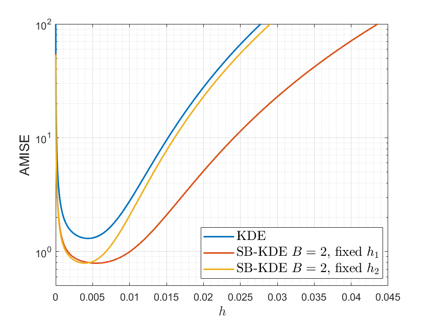
Figure 1: AMISE vs. bandwidth for KDE and SB-KDE. Notice that, being AMISE a function of $B=2$ bandwidths for SB-KDE, curves are obtained by fixing one bandwidth value and varying the other. We assumed $S_{\rm max}=100$, and true p.d.f. with $\bm{h}=[1.5,2.7,1.2]$.

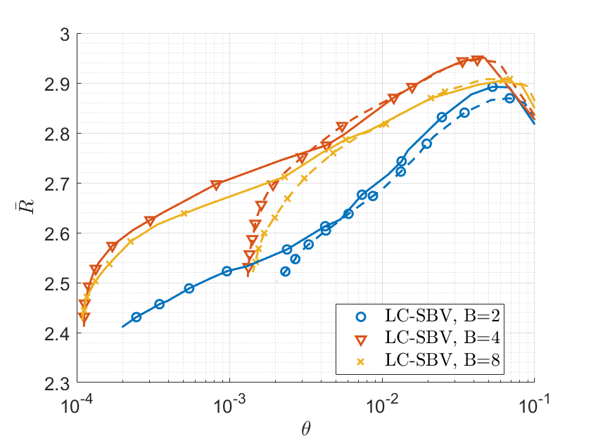
(a) LC-SB V

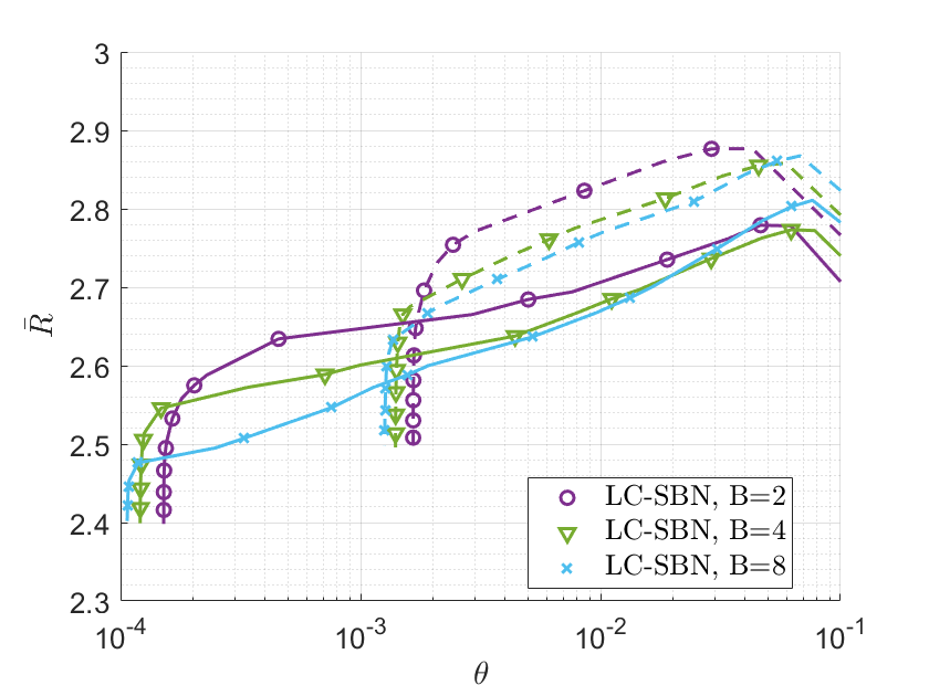
(b) LC-SB N

Figure 2: Average DR vs. $\theta$ for LC-SB V (left) and LC-SB N (right). In both figures same marker denotes the same number of subsets. Results are reported for a training set of $L=10^{3}$ samples (dashed lines) and a training set of $L=10^{4}$ samples (solid lines).

VI Numerical Results

VI-A SB-KDE Optimality

In order to assess the performance of the SB-KDE density estimator, we compare the AMISE obtained for both KDE and SB-KDE for a fixed and known p.d.f. $f(x)$ of a random variable. In particular, we assume that the true p.d.f. is given by (22) for $B=3$ and $\bm{h}=[1.5,2.7,1.2]$. This allows us to compute the p.d.f. $f(x)$ for each $x$ in a predefined dataset $\mathcal{S}$. We assume that $\mathcal{S}=\{0,1,\ldots,S_{\rm max}\}$, and we randomly create sets $\mathcal{X}_{i}$, $i=1,\ldots,B$, such that $\bigcup\limits_{i=1}^{B}\mathcal{X}_{i}=\mathcal{S}$.

Fig. 1 shows the AMISE obtained with KDE as in (16) and SB-KDE as in (25) with $B=2$. Notice that both estimates are approximations of the true p.d.f., which is based on $3$ subsets. Furthermore, since the AMISE for SB-KDE is a function of two bandwidths, results are shown by fixing one bandwidth to the optimal value, and letting the other vary. By using multiple bandwidths, the AMISE is reduced, validating our approach. Furthermore, we notice that the proposed solution is less sensitive to sub-optimal bandwidth values. In fact, we notice that near-to-optimal AMISE values are obtained for a wider range of bandwidth values for SB-KDE with rspect to KDE.

VI-B Link Adaptation

In this work, we assume that the LA can match the FT-BER target if the predicted IP is larger than that experienced at transmission time. Therefore, we assume a correct transmission if the predicted IP is larger than the actual one at the successive time instant, whereas otherwise a failure occurs. This models a system where uncontrolled re-transmissions are to be avoided, for instance due to very strict latency constraints in URLLC. For each IP test sequence of $T$ TTIs, we evaluate the reliability of the different solutions by counting the number of events in which the predicted IP is below the actual one. We hence define the reliability of the system (between $0$ and $1$) as

$$1-\theta=1-\frac{\sum_{t=1}^{T-1}\chi(t)}{T-1},$$ (37)

where $\chi(t)$ is the indicator function

$$\chi(t)=\begin{cases}1\quad{\rm if}\,\hat{\phi}(t)<\phi(t);\\ 0\quad{\rm otherwise}.\end{cases}$$ (38)

Notice that, $\theta$ represents the unreliability. Since we are interested in high reliability, we aim at small $\theta$ values.

For each UE we assume that, if a failure happens, the experienced DR is zero, due to the packet’s transmission’s failure. Therefore, considering short packets of size $M$, the instantaneous DR $R(t)$ at TTI $t$ is [25]

$$R(t)\approx(1-\chi(t))\left(\log_{2}(1+\hat{\rho}(t))-\sqrt{\frac{1}{M}V(\hat{\rho}(t))}Q^{-1}(\varepsilon)\right),$$ (39)

where $V(\hat{\rho}(t))=\frac{\hat{\rho}(t)(2+\hat{\rho}(t))}{(1+\hat{\rho}(t))^{2}}$, where $Q$ is the Gaussian complementary CDF, $Q^{-1}$ is its inverse, and $\hat{\rho}(t)$ is the predicted SINR. We denote as $\bar{R}$ the average DR in time, and as $M=128$ the number of channel uses. Notice that we used $\approx$ in (39) as we neglect terms with $O(\log M/M)$.

For the MQ-based methods, we consider that prediction exploits the conditional p.d.f. (11), where prediction is based on the previous measured IP, i.e., $N_{\rm prev}=1$.

We compare two different heuristic policies for creating LC-SB subsets. The first is based on the values assumed by the IPs in the time series. In particular, assuming an IP sequence with minimum value $m$ and maximum value $M$, the $b^{\rm th}$ subset is given by $\mathcal{X}^{(b)}_{d}=x_{d},\,{\rm s.t.}\,x_{d}\geq(b-1)\frac{M-m}{B}+1\,{\rm and}\,x_{d}<b\frac{M-m}{B}$. We denote this method by LC-SB V. The latter policy is based on the number of different IPs in the time series. In particular, we populate each subset with the same number of sample points. We denote this method as LC-SB N.

VI-C Baseline Algorithms

In order to better assess the performance of the SB-KDE and its low-complexity version, we compare the results with four state-of-the-art algorithms. Two baselines are given by the MQ method proposed in [13], based on the empirical CDF (13) (henceforth referred to as ECDF) and on KDE. The third method is the based on OLLA, described in Section II. Since OLLA does not exploit any interference prediction method, for a fair comparison, we exploit the low-pass filtering of the IPs proposed in [7]. We will hereafter denote this method as OLLA-LPP. In particular, given the previously predicted IP $\hat{\phi}(t)$ and the current measured IP $\phi(t)$, the IP to be used for the next transmission is given by [7]

$$\hat{\phi}(t+1)=\alpha\phi(t)+(1-\alpha)\hat{\phi}(t-1),$$ (40)

where $\alpha$ is a constant real value, which is usually small. The predicted value is then used to compute the SINR $\rho_{OLLA}^{(t+1)}$. The last baseline method assumes the IPs’ distribution to be log-normal. Its first and second (order) moments are estimated as a log-normal random variable [26]. We propose to set the first and second moments of the p.d.f. as the mean $\mu_{\bm{\mathcal{X}}}$ and variance $\sigma^{2}_{\bm{\mathcal{X}}}$ of the training set given by $\bm{\mathcal{X}}$. The predicted IP is hence given by

$$\hat{\phi}(t+1)=\exp\left(\Theta^{-1}\left(2\varepsilon-1\right)\sqrt{2}\sigma_{\bm{\mathcal{X}}}+\mu_{\bm{\mathcal{X}}}\right),$$ (41)

where $\Theta(x)$ represents the error function

$$\Theta(x)=\frac{1}{\sqrt{\pi}}\int_{-x}^{x}e^{-t^{2}}dt.$$ (42)

VI-D Rice Channel Model

We here consider a scenario with $N=9$ square cells, with each gNB located at the center of is at a distance of $200$ m from neighboring gNBs. Each gNB is equipped with $N_{a}=16$ antennas linearly spaced by $d=\lambda/2$. The IPs are measured in the central cell, and the number of UEs in each surrounding cell is given by the realization of a uniform random variable in range $[2,8]$. We consider a noise power of $\sigma^{2}=-101$ dBm, a transmitted power at each gNB of $P=46$ dBm, Rice $K$ factor $\Psi=10$ dB, path loss exponent $\nu=3.5$ and a cell edge signal to noise ratio (SNR) without interference of $20$ dB. This corresponds to a typical highly interference limited scenario in practical deployments [15].

Fig. 2 shows the average DR vs. $\theta$ for the LC-SB V (left) and LC-SB N (right). Results have been obtained by fixing the number $L$ of training samples used for p.d.f. estimation and changing the parameter $\varepsilon$, yielding different values of $\theta$. Figures show both the impact of increasing $L$ and the effect of the number of subsets $B$. About the sensitivity with respect to $L$, we denote with dashed line the results obtained estimating the p.d.f. with $L=10^{3}$ samples and with solid line the results obtained estimating the p.d.f. with $L=10^{4}$ samples. Moreover, for each curve in each figure, a higher reliability, i.e., la smaller $\theta$, is obtained by decreasing $\varepsilon$. We notice that a larger $L$ leads to a higher reliability with both policies, since having a larger number of training samples yields a higher precision in the estimated p.d.f.. We also notice that for LC-SB N a lower $L$ leads to higher DR for high $\theta$. Indeed, a lower precision in the p.d.f. estimation leads to a less conservative behavior, with higher rates and a lower reliability. We now consider the effect of the number of subsets. We notice that more subsets entail a lower $\theta$ and hence a higher reliability for both policies, whereas in terms of rate results do not show the same behavior. In fact, for LC-SB V the best trade-off between DR and reliability is obtained when considering $B=4$ subsets, whereas for LC-SB N is obtained with $B=2$ subsets. We can hence identify the number of subsets as a hyper-parameter, to be optimized based on collected data. Comparing the two policies, we notice that LC-SB V attains higher DR as the reliability increases. In the following, we choose LC-SB V $B=4$ as the policy to be compared with baseline algorithms, as it achieves the best performance both in terms of average DR and reliability.

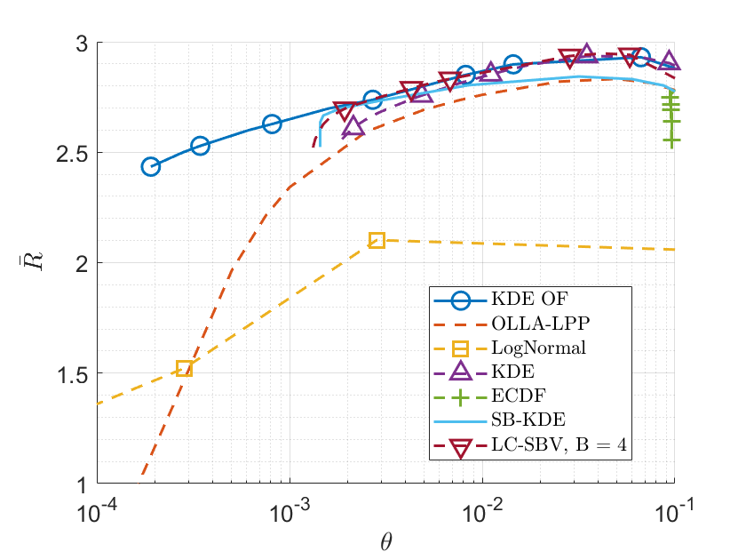
Figure 3: Average DR vs. $\theta$ for the best performing policy chosen from Fig. 2 and the baseline methods. Estimation performed with $L=10^{3}$ samples.

Fig. 3 shows the average DR vs. $\theta$ for the best policy chosen from Fig. 2 and the baseline methods, when considering $L=10^{3}$ training samples. For KDE we show both the performance obtained with $L=10^{3}$ training samples and the optimal results obtained by over-fitting, i.e., using all samples in the dataset for training. The ECDF method based on (13) attains a poor approximation of the CDF, since not enough points are available to match the strict reliability targets. The comparison with the other methods motivates the need for kernel-based density estimators. About OLLA-LPP we notice that, although it works well with high $\theta$ values, the attained DR rapidly degrades for decreasing $\theta$, due to the highly conservative behavior of OLLA which favors reliability to DR. Considering a URLLC scenario targeting high reliability, and hence small $\theta$, we notice that OLLA-LPP is not able to guarantee both high reliability and high DR, therefore not being a suitable solution if the load offered by URLLC becomes relevant. A similar behavior is obtained with the LogNormal approximation, where DR rapidly degrades with increasing reliability values. However, differently from OLLA-LPP, the DR has a slower decrease and does not tend to zero for $\theta<10^{-4}$. Furthermore, we notice that, compared to the other p.d.f.-based methods, LogNormal reaches smaller values of $\theta$. Indeed, this method relies on a closed-form equation of the IP p.d.f. and does not suffer for an insufficient number of training data, being able to reach infinite precision. On the other hand, we notice that the LogNormal approximation attains a higher DR than OLLA-LPP for $\theta<2\cdot 10^{-4}$. The DR for the proposed SB-KDE degrades as $\theta$ decreases. However, it attains a higher DR when it’s able to match the desired reliability when compared to LogNormal and OLLA-LPP, whereas, when compared to KDE, it attains higher DR only for $\theta\leq 5\cdot 10^{-3}$. Furthermore, compared to KDE, it also to attains lower $\theta$, for $\theta\leq 2\cdot 10^{-3}$, confirming that a subset-based approach is advantageous over the plain KDE. Comparing the low-complexity LC-SB V with all other approaches, we notice that it attains the highest DR for all $\theta\geq 2\cdot 10^{-3}$. However, LC-SBV is limited by the demanding amount of data needed to estimate the p.d.f..

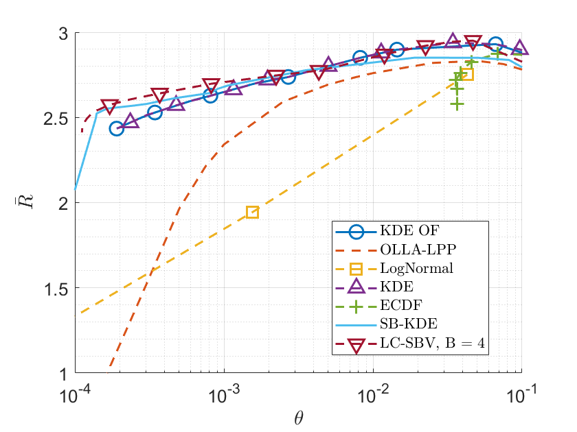
Figure 4: Average DR vs. $\theta$ for the best performing policy chosen from Fig. 2 and the baseline methods. Estimation performed with $L=10^{4}$ samples.

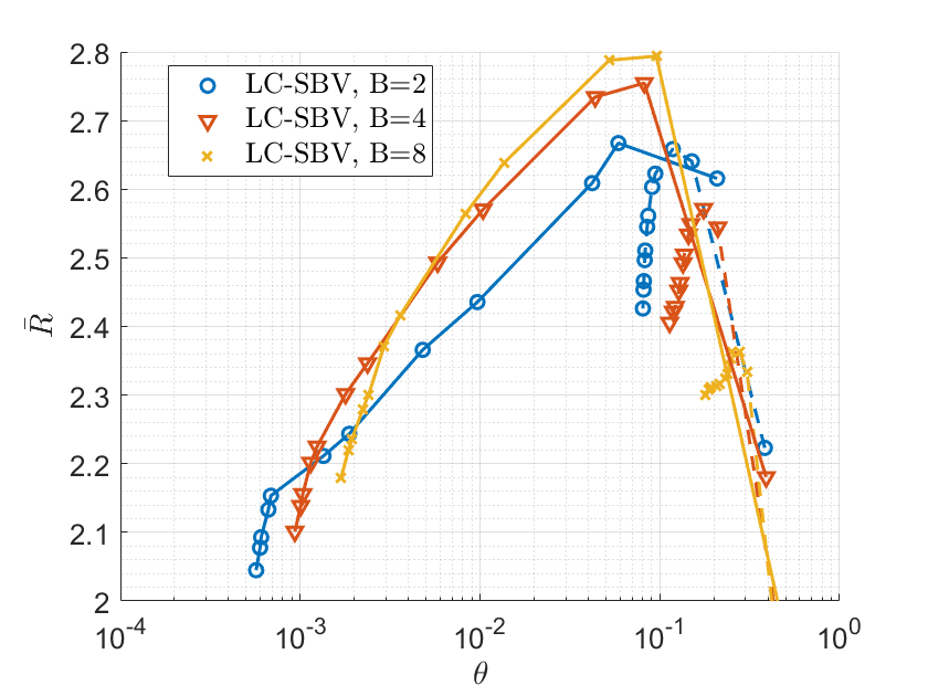
(a) LC-SB V

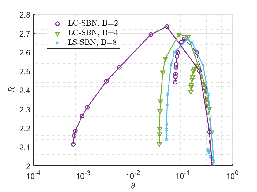
(b) LC-SB N

Figure 5: DR vs. $\theta$ for LC-SB V (left) and LC-SB N (right) obtained with the 3GPP channel model. In both figures same marker shape denotes the same number of subsets. Results are reported for a training set of $L=10^{2}$ samples (dashed lines) and a training set of $L=10^{4}$ samples (solid lines).

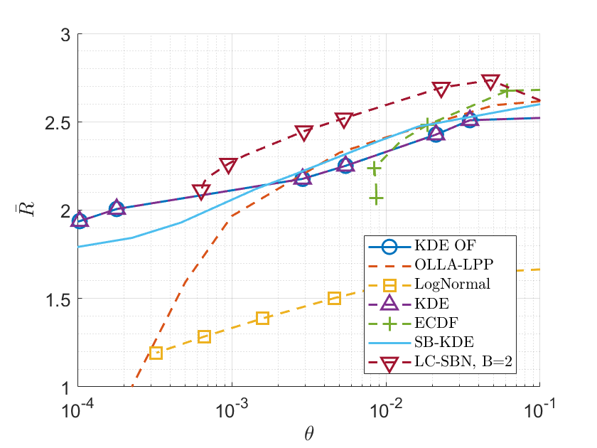
Figure 6: Average DR vs. $\theta$ for the best performing policy chosen from Fig. 5 and the baseline methods. Results obtained with $L=10^{4}$ training samples.

Fig. 4 shows the average DR vs $\theta$, for the best performing policy chosen from Fig. 2 and the baseline methods, when considering $L=10^{4}$ training samples. Note that both KDE approaches have similar performance, i.e., convergence is already obtained with $10^{4}$ training samples. For the ECDF method, a larger training set does not improve its performance. About SB-KDE, we notice a DR degradation smaller than $0.2$ bit/s/Hz, up to $\theta=0.5\cdot 10^{-4}$, then DR rapidly decreases, still being higher than that of OLLA-LPP and that of Log-normal approximation. Furthermore, we also notice that the subset-based approaches attain smaller $\theta$ values than KDE, and LC-SB V is the best performing method down to $\theta=10^{-4}$.

VI-E 3GPP Channel Model

In order to test the proposed algorithm in a more realistic scenario, we consider in this section a three-dimensional spatial 3D Urban Micro (UMi) channel, calibrated with the results obtained by 3GPP [15]. In detail, we consider $C=21$ cells, organized in $7$ sites, each with $120$ degrees subsets per cell, inter-site distance of $200$ m, and wraparound. An average of $5$ UEs is deployed per cell, which move with a speed of $3$ km/h. Each gNB is equipped with $64$ antennas, organized in a uniform planar array, with $8$ rows, $4$ columns and with cross-polarized antenna elements. The gNBs serve UEs at a carrier frequency of $3.7$ GHz on a system bandwidth of $10$ MHz and using a transmit power of $41$ dBm. We follow the scenario in [15], where the reader can find more details.

Results have been obtained by fixing the number $L$ of training samples for p.d.f. estimation and varying $\varepsilon$, allowing to obtain different $\theta$ values. As for the Rice channel model, we show both the effect of increasing $L$ and varying the number $B$ of subsets.

Fig. 5 shows the DR vs. $\theta$ for the two considered policies for the LC-SB algorithm. Dashed lines refer to training sequences of $L=10^{2}$ samples, while solid lines to training sequences of $10^{4}$ samples. We notice that, if the training set does not have enough samples, both methods are unable to attain small $\theta$ values with a poor reliability. About LC-SB V, we notice the trade-off between DR and reliability when considering the number of subsets $B$ needed to estimate the p.d.f.. In fact, on one hand a larger number of subsets yields higher DR values, on the other hand a smaller number of subsets means we reach smaller $\theta$ values. Hence, this parameter will be set according to the specific users’ need. About LC-SB N, we instead notice that increasing the number of subsets does not improve performance. However, the LC-SB N with $B=2$ is the best performing method among all policies and number of subsets, and is hence compared with the baseline methods.

Fig. 6 shows the average DR vs. $\theta$ for all the baseline methods, the proposed SB-KDE and LC-SB N with $B=2$ subsets. Results are obtained with $L=10^{4}$ training samples. As for Fig. 4, both OLLA-LP and the LogNormal approximation attain decreasing DR values for decreasing $\theta$. Regarding KDE, performance obtained considering $10^{4}$ training samples is equal to those obtained considering the full dataset, meaning that convergence has been reached. However we recall that, although these are the best results obtainable with KDE, they do not represent the overall optimum, as the estimated p.d.f. may be inaccurate. In fact, with ECDF we attain higher DRs for high $\theta$ values. However, KDE can reach $\theta=10^{-4}$, showing that kernel methods provide good performance for low reliability target. About the proposed SB-KDE, it achieves higher DR values compared to those of KDE for $\theta>2\cdot 10^{-3}$, whereas LC-SB N attains higher DR values for all $\theta\geq 6\cdot 10^{-4}$, as LC-SB N can not attain lower $\theta$ values considering $L=10^{4}$ training samples.

Fig. 7 shows the computational complexity in terms of number of additions and multiplications vs. the number of training samples $L$ for the KDE and the two policies for the low-complexity LC-SB. The best performing method is the LC-SB N, due to the fact that it linearly depends on the number of samples per subset, which decreases as the number of subset increases.

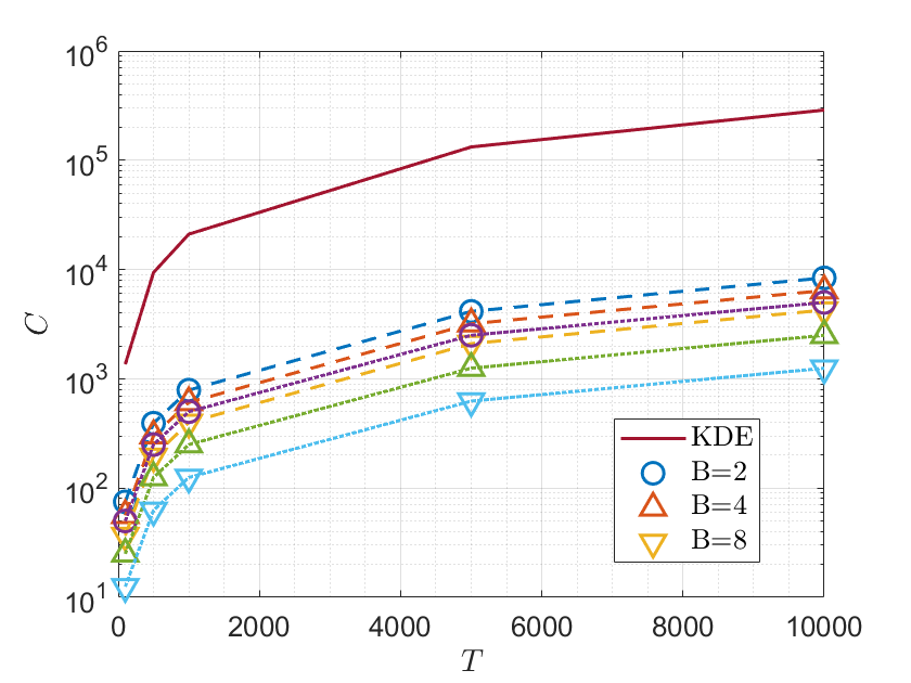
Figure 7: Computational complexity vs. number of training data for the kernel based density estimators. Dashed curves show results for LC-SB V, whereas dotted curves show results for LC-SB N.

VII Conclusions

In this paper we considered the problem of predicting interference power to enable efficient link adaptation for URLLC. We considered variable bandwidth kernel density estimators. We first derived the optimal bandwidth for the SB-KDE, and based on the optimal solution for KDE, we proposed a heuristic algorithm to estimate a p.d.f. based on the optimal bandwidths. Motivated by the considerable computational complexity of the proposed solution, we then proposed a low-complexity version of the SB-KDE, namely the LC-SB. By means of extensive simulations in cellular networks, considering realistic 3GPP 3D UMi channel models, we showed through numerical evaluations that the proposed solutions attain at the same time higher DR a better and matching of the reliability targets than state-of-the-art solutions. By jointly looking at results in Fig.s 4,6 and 7, we can conclude that the proposed LC-SB method attains the best DR with the lower computational complexity and achieves extremely high reliability targets. Therefore, it is the best investigated algorithm for URLLC, being hence an effective approach to LA.

Appendix A Derivation of the Optimal Bandwidth for SB-KDE

We henceforth consider operations between vector and scalar as element-wise. We also recall that the kernel function of a vector is a scalar value. We assume that $K(\cdot)$ is a kernel function as defined in [14], therefore $\int K(u)du=1$ and that $\int uK(u)du=0$.

A-A Bias

Define the local KDE as

$$\hat{f}(\bm{x})=\frac{1}{B}\sum_{i=1}^{B}\frac{1}{|\bm{\mathcal{X}}_{i}|}\sum_{\bm{z}\in\bm{\mathcal{X}}_{i}}\frac{1}{h_{i}}K\left(\frac{\bm{z}-\bm{x}}{h_{i}}\right).$$ (43)

The mean value of the kernel function can be computed as

$$\begin{split}&E\left[\frac{1}{h_{i}}K\left(\frac{\bm{z}-\bm{x}}{h_{i}}\right)\right]=\int_{-\infty}^{\infty}\frac{1}{h_{i}}K\left(\frac{\bm{\zeta}-\bm{x}}{h_{i}}\right)f(\bm{\zeta})d\bm{\zeta}.\\ \end{split}$$ (44)

From the total probability law we have

$$f(\bm{\zeta})=\sum_{\ell=1}^{B}f(\bm{\zeta}|\bm{\mathcal{X}}_{\ell})\mathbb{P}(\bm{\mathcal{X}}_{\ell}),$$ (45)

and by substitution in (44) we obtain

$$\begin{split}&E\left[\frac{1}{h_{i}}K\left(\frac{\bm{z}-\bm{x}}{h_{i}}\right)\right]=\\ &\int_{-\infty}^{\infty}\frac{1}{h_{i}}K\left(\frac{\bm{\zeta}-\bm{x}}{h_{i}}\right)\sum_{\ell=1}^{B}f(\bm{\zeta}|\bm{\mathcal{X}}_{\ell})\mathbb{P}(\bm{\mathcal{X}}_{\ell})d\bm{\zeta}.\\ \end{split}$$ (46)

By performing the change of variables $\bm{u}=(\bm{z}-\bm{x})/h_{i}$ we obtain

$$\begin{split}&E\left[\frac{1}{h_{i}}K\left(\frac{\bm{z}-\bm{x}}{h_{i}}\right)\right]=\\ &\int_{-\infty}^{\infty}K\left(\bm{u}\right)\sum_{\ell=1}^{B}f(\bm{u}h_{i}+\bm{x}|\bm{\mathcal{X}}_{\ell})\mathbb{P}(\bm{\mathcal{X}}_{\ell})d\bm{u}.\end{split}$$ (47)

Let us consider the second order Taylor series expansion of $f(\bm{u}h_{i}+x|\bm{\mathcal{X}}_{i})$, obtaining

$$\begin{split}&f(\bm{u}h_{i}+\bm{x}|\bm{\mathcal{X}}_{i})\approx f(\bm{x}|\bm{\mathcal{X}}_{i})+f^{(1)}(\bm{x}|\bm{\mathcal{X}}_{i})h_{i}\bm{u}+\\ &\frac{1}{2}f^{{}^{\prime\prime}}(\bm{x}|\bm{\mathcal{X}}_{i})h_{i}^{2}\bm{u}^{2}+o(h_{i}^{2}).\end{split}$$ (48)

By substitution of (48) in (47) we obtain

$$\sum_{\ell=1}^{B}\int_{-\infty}^{\infty}K\left(\bm{u}\right)f(\bm{u}h_{i}+\bm{x}|\bm{\mathcal{X}}_{i})\mathbb{P}(\bm{\mathcal{X}}_{\ell})d\bm{u}=$$ (49)

$$\sum_{\ell=1}^{B}\int_{-\infty}^{\infty}K\left(\bm{u}\right)\big{(}f(\bm{x}|\bm{\mathcal{X}}_{\ell})+f^{(1)}(\bm{x}|\bm{\mathcal{X}}_{\ell})h_{\ell}\bm{u}+$$ (50)

$$\frac{1}{2}f^{{}^{\prime\prime}}(\bm{x}|\bm{\mathcal{X}}_{\ell})h_{\ell}^{2}\bm{u}^{2}\big{)}\mathbb{P}(\bm{\mathcal{X}}_{\ell})d\bm{u}=$$

$$\sum_{\ell=1}^{B}\left(f(\bm{x}|\bm{\mathcal{X}}_{\ell})+\frac{1}{2}f^{{}^{\prime\prime}}(\bm{x}|\bm{\mathcal{X}}_{\ell})h_{\ell}^{2}\omega_{2}(K)\right)\mathbb{P}(\bm{\mathcal{X}}_{\ell}),$$

where the second term involving the first derivative is zero as the mean of $K(\bm{u})$ is zero and where $\omega_{2}(K)$ is defined in (24).

Therefore

$$E[\hat{f}(\bm{x})]=E\left[\frac{1}{B}\sum_{i=1}^{B}\frac{1}{|\bm{\mathcal{X}}_{i}|}\sum_{\bm{z}\in\bm{\mathcal{X}}_{i}}\frac{1}{h_{i}}K\left(\frac{\bm{z}-\bm{x}}{h_{i}}\right)\right]$$

$$=\frac{1}{B}\sum_{i=1}^{B}\frac{1}{|\bm{\mathcal{X}}_{i}|}\sum_{\bm{z}\in\bm{\mathcal{X}}_{i}}E\left[\frac{1}{h_{i}}K\left(\frac{\bm{z}-\bm{x}}{h_{i}}\right)\right]$$

$$=\frac{1}{B}\sum_{i=1}^{B}\frac{1}{|\bm{\mathcal{X}}_{i}|}\sum_{\bm{z}\in\bm{\mathcal{X}}_{i},\ell=1}^{B}\left(f(\bm{x}|\bm{\mathcal{X}}_{\ell})+\frac{1}{2}f^{{}^{\prime\prime}}(\bm{x}|\bm{\mathcal{X}}_{\ell})h_{\ell}^{2}\omega_{2}(k)\right)\mathbb{P}(\bm{\mathcal{X}}_{\ell})$$

$$=f(\bm{x})+\frac{1}{B}\sum_{i=1}^{B}\left(\sum_{\ell=1}^{B}\frac{1}{2}f^{{}^{\prime\prime}}(\bm{x}|\bm{\mathcal{X}}_{\ell})h_{\ell}^{2}\omega_{2}(k)\mathbb{P}(\bm{\mathcal{X}}_{\ell})\right)$$

$$=f(\bm{x})+\sum_{\ell=1}^{B}\frac{1}{2}f^{{}^{\prime\prime}}(\bm{x}|\bm{\mathcal{X}}_{\ell})h_{\ell}^{2}\omega_{2}(k)\mathbb{P}(\bm{\mathcal{X}}_{\ell}).$$

Therefore, the bias is

$${\rm Bias}(\hat{f}(\bm{x}))=E[\hat{f}(\bm{x})]-f(\bm{x})$$ (51)

$$=\omega_{2}(k)\sum_{\ell=1}^{B}\frac{1}{2}f^{{}^{\prime\prime}}(\bm{x}|\bm{\mathcal{X}}_{\ell})h_{\ell}^{2}\mathbb{P}(\bm{\mathcal{X}}_{\ell})+o(h_{i}^{2}).$$

A-B Variance

From the bias analysis we saw how the kernel function of a vector can be treated as a random variable. The variance of a random variable (r.v.) $x$ can be computed as

$${\rm Var}(x)=E[x^{2}]-E[x]^{2}.$$ (52)

From the bias analysis, focusing on the first order Taylor approximation we have

$$E[\hat{f}(\bm{x})]\approx f(\bm{x})+o(1),$$ (53)

where the second term is $O\left(\frac{1}{N}\right)$, being $N$ the number of samples used for density estimation. Then, following the approach used for the bias computation we have

$$E\left[\frac{1}{h_{i}}K\left(\frac{\bm{z}-\bm{x}}{h_{i}}\right)^{2}\right]=$$ (54)

$$\frac{1}{h_{i}}\int_{-\infty}^{\infty}K\left(\bm{u}\right)^{2}\sum_{\ell=1}^{B}f(\bm{u}h_{i}+\bm{x}|\bm{\mathcal{X}}_{\ell})\mathbb{P}(\bm{\mathcal{X}}_{\ell})d\bm{u}$$ (55)

$$=\int_{-\infty}^{\infty}K\left(\bm{u}\right)^{2}f(\bm{u}h_{i}+\bm{x})d\bm{u},$$

where the second equality comes from the fact that we considered a first order Taylor series and the total probability law. Therefore, recalling that the kernel estimator is a linear estimator and that $K\left(\frac{\bm{z}-\bm{x}}{h_{i}}\right)$ is independent identically distributed (i.i.d)

$${\rm Var}(\hat{f}(\bm{x}))$$ (56)

$$=\frac{1}{B^{2}}\sum_{i=1}^{B}\frac{1}{|\bm{\mathcal{X}}_{i}|^{2}}\sum_{\bm{z}\in\bm{\mathcal{X}}_{i}}\frac{1}{h_{i}}\Upsilon(K)f(\bm{x})+O\left(\frac{1}{N}\right),$$

$$=\Upsilon(K)f(\bm{x})\frac{1}{B^{2}}\sum_{i=1}^{B}\frac{1}{|\bm{\mathcal{X}}_{i}|h_{i}}+O\left(\frac{1}{N}\right),$$

where $\Upsilon(K)$ is defined in (17).

A-C AMISE

The MSE can be expressed as

$${\rm MSE}={\rm Bias}(\hat{f}(\bm{x}))^{2}+{\rm Var}(\hat{f}(\bm{x})).$$ (57)

The asymptotic mean squared error (AMSE) is obtained by the asymptotic derivation of bias and variance (51) and (56) as

$$\begin{split}&{\rm AMSE}=\left(\frac{1}{2}\omega_{2}(K)\sum_{i=1}^{B}f^{{}^{\prime\prime}}(\bm{x}|\bm{\mathcal{X}}_{i})h_{i}^{2}\mathbb{P}(\bm{\mathcal{X}}_{i})\right)^{2}\\ &+\Upsilon(K)f(\bm{x})\frac{1}{B^{2}}\sum_{i=1}^{B}\frac{1}{|\bm{\mathcal{X}}_{i}|h_{i}}.\end{split}$$

By integrating the AMSE we obtain the AMISE

$$\begin{split}&{\rm AMISE}\\ &=\int_{-\infty}^{\infty}\left[\left(\frac{1}{2}\omega_{2}(K)\sum_{i=1}^{B}f^{{}^{\prime\prime}}(\bm{x}|\bm{\mathcal{X}}_{i})h_{i}^{2}\mathbb{P}(\bm{\mathcal{X}}_{i})\right)^{2}\right.+\\ &\left.\Upsilon(K)f(\bm{x})\frac{1}{B^{2}}\sum_{i=1}^{B}\frac{1}{|\bm{\mathcal{X}}_{i}|h_{i}}\right]d\bm{x}.\end{split}$$ (58)

Since $f(\bm{x}|\bm{\mathcal{X}}_{i})=0\,\forall\bm{x}\notin\bm{\mathcal{X}}_{i}$ we obtain

$$\begin{split}&{\rm AMISE}\\ &=\int_{-\infty}^{\infty}\left(\frac{1}{4}\omega_{2}(k)^{2}\sum_{i=1}^{B}f^{{}^{\prime\prime}}(\bm{x}|\bm{\mathcal{X}}_{i})^{2}h_{i}^{4}\mathbb{P}(\bm{\mathcal{X}}_{i})^{2}\right.\\ &\left.+\Upsilon(K)f(\bm{x})\frac{1}{B^{2}}\sum_{i=1}^{B}\frac{1}{|\bm{\mathcal{X}}_{i}|h_{i}}\right)d\bm{x}\\ &=\sum_{i=1}^{B}\left(\frac{1}{4}\Upsilon(f^{{}^{\prime\prime}}(\bm{x}|\bm{\mathcal{X}}_{i}))h_{i}^{4}\mathbb{P}(\bm{\mathcal{X}}_{i})^{2}\omega_{2}(k)^{2}+\frac{\Upsilon(K)}{B^{2}|\bm{\mathcal{X}}_{i}|h_{i}}\right).\end{split}$$

A-D Optimal bandwidth

The optimal value $h_{i}^{*}$ can be computed as

$$\frac{\partial{\rm AMISE}}{\partial h_{i}} =\Upsilon(f^{{}^{\prime\prime}}(\bm{x}|\bm{\mathcal{X}}_{i}))h_{i}^{3}\mathbb{P}(\bm{\mathcal{X}}_{i})^{2}\omega_{2}(K)^{2}-\frac{\Upsilon(K)}{B^{2}|\bm{\mathcal{X}}_{i}|h_{i}^{2}}$$

$$=0,$$

from which the AMISE optimal bandwidth value is given by

$$h_{i}^{*}=\left(\frac{\Upsilon(K)}{B^{2}|\bm{\mathcal{X}}_{i}|\Upsilon(f^{{}^{\prime\prime}}(\bm{x}|\bm{\mathcal{X}}_{i}))\mathbb{P}(\bm{\mathcal{X}}_{i})^{2}\rho_{2}(k)^{2}}\right)^{\frac{1}{5}}.$$ (59)

Considering a Gaussian kernel we have

$${\rm AMISE}$$ (60)

$$=\frac{1}{4}\sum_{i=1}^{B}\left(\Upsilon(f^{{}^{\prime\prime}}(\bm{x}|\bm{\mathcal{X}}_{i}))h_{i}^{4}\mathbb{P}(\bm{\mathcal{X}}_{i})^{2}+\frac{1}{B^{2}|\bm{\mathcal{X}}_{i}|2\sqrt{\pi}h_{i}}\right),$$

and therefore

$$h_{i}^{*}=\left(\frac{1}{2B^{2}|\bm{\mathcal{X}}_{i}|\sqrt{\pi}\Upsilon(f^{{}^{\prime\prime}}(\bm{x}|\bm{\mathcal{X}}_{i}))\mathbb{P}(\bm{\mathcal{X}}_{i})^{2}}\right)^{\frac{1}{5}}.$$ (61)

References

- [1] H. Ren, C. Pan, Y. Deng, M. Elkashlan, and A. Nallanathan, “Joint power and blocklength optimization for URLLC in a factory automation scenario,” IEEE Trans. on Wireless Commun., vol. 19, no. 3, pp. 1786–1801, Dec. 2019.
- [2] X. Ge, “Ultra-reliable low-latency communications in autonomous vehicular networks,” IEEE Trans. on Vehicular Technology, vol. 68, no. 5, pp. 5005–5016, Mar. 2019.
- [3] K. S. Kim et al., “Ultrareliable and low-latency communication techniques for tactile internet services,” Proceedings of the IEEE, vol. 107, no. 2, pp. 376–393, Feb. 2018.
- [4] M. Shirvanimoghaddam et al., “Short block-length codes for ultra-reliable low latency communications,” IEEE Communications Magazine, vol. 57, no. 2, pp. 130–137, Dec. 2018.
- [5] Z. Zhou, R. Ratasuk, N. Mangalvedhe, and A. Ghosh, “Resource allocation for uplink grant-free ultra-reliable and low latency communications,” in Proc. 87th Vehicular Technology Conference (VTC Spring), Jul. 2018, pp. 1–5.
- [6] Z. Li, M. A. Uusitalo, H. Shariatmadari, and B. Singh, “5G URLLC: Design challenges and system concepts,” in Proc. Inte. Symp. on Wireless Commun. Systems (ISWCS), Aug. 2018, pp. 1–6.
- [7] G. Pocovi, K. I. Pedersen, and P. Mogensen, “Joint link adaptation and scheduling for 5G ultra-reliable low-latency communications,” IEEE Access, vol. 6, pp. 28 912–28 922, 2018.
- [8] G. Pocovi, A. A. Esswie, and K. I. Pedersen, “Channel quality feedback enhancements for accurate URLLC link adaptation in 5g systems,” in Proc. Vehicular Technology Conf. (VTC2020-Spring), May 2020, pp. 1–6.
- [9] H. Shariatmadari, Z. Li, M. A. Uusitalo, S. Iraji, and R. Jäntti, “Link adaptation design for ultra-reliable communications,” in Proc. International Conference on Communications (ICC), May 2016, pp. 1–5.
- [10] L. Buccheri, S. Mandelli, S. Saur, L. Reggiani, and M. Magarini, “Hybrid retransmission scheme for QoS-defined 5G ultra-reliable low-latency communications,” in Proc. IEEE Wireless Commun. and Networking Conf. (WCNC), Apr. 2018, pp. 1–6.
- [11] A. Belogaev, E. Khorov, A. Krasilov, D. Shmelkin, and S. Tang, “Conservative link adaptation for ultra reliable low latency communications,” in Proc. International Black Sea Conference on Communications and Networking (BlackSeaCom), Jun. 2019, pp. 1–5.
- [12] M. Deghel, S. E. Elayoubi, A. Galindo-Serrano, and R. Visoz, “Joint optimization of link adaptation and harq retransmissions for URLLC services,” in Proc. 25th International Conference on Telecommunications (ICT), Jun. 2018, pp. 21–26.
- [13] A. Brighente, J. Mohammadi, and P. Baracca, “Interference distribution prediction for link adaptation in ultra-reliable low-latency communications,” in Proc. 91st Vehicular Technology Conference (VTC2020-Spring), May 2020, pp. 1–7.
- [14] E. Parzen, “On estimation of a probability density function and mode,” The annals of mathematical statistics, vol. 33, no. 3, pp. 1065–1076, Sep. 1962.
- [15] 3GPP, “TR 138 901 V14.0.0, study on channel model for frequencies from 0.5 to 100 GHz,” 3GPP, Tech. Rep., May 2017.
- [16] D. Tse and P. Viswanath, Fundamentals of wireless communication. Cambridge university press, 2005.
- [17] 3GPP, “TS 22 104 V17.4.0, service requirements for cyber-physical control applications in vertical domains,” 3GPP, Tech. Rep., Sep. 2020.
- [18] ——, “TR 138 901 V15.3.0, physical layer procedures for data,” 3GPP, Tech. Rep., Oct. 2018.
- [19] A. Sampath, P. S. Kumar, and J. M. Holtzman, “On setting reverse link target SIR in a CDMA system,” in Proc. Vehicular Technology Conf. (VTC), vol. 2, May 1997, pp. 929–933.
- [20] Z. I. Botev, J. F. Grotowski, D. P. Kroese et al., “Kernel density estimation via diffusion,” The annals of Statistics, vol. 38, no. 5, pp. 2916–2957, Aug. 2010.
- [21] G. R. Terrell and D. W. Scott, “Variable kernel density estimation,” The Annals of Statistics, pp. 1236–1265, 1992.
- [22] T. M. Cover, Elements of information theory. John Wiley & Sons, 1999.
- [23] G. Plonka and M. Tasche, “Fast and numerically stable algorithms for discrete cosine transforms,” Linear algebra and its applications, vol. 394, pp. 309–345, Jan. 2005.
- [24] R. L. Burden and D. J. Faires, Numerical analysis. PWS Publishing Company, 1985.
- [25] Y. Polyanskiy, H. V. Poor, and S. Verdú, “Channel coding rate in the finite blocklength regime,” IEEE Trans. on Information Theory, vol. 56, no. 5, pp. 2307–2359, May 2010.
- [26] K. Sung, H. Haas, and McLaughlin, “A semianalitical PDF of downlink SINR for femtocell networks,” EURASIP Journal on Wireless Comm. and Networking, pp. 1–9, Feb. 2010.