Bonded discrete element simulations of sea ice with non-local failure: Applications to Nares Strait
Abstract
The discrete element method (DEM) can provide detailed descriptions of sea ice dynamics that explicitly model floes and discontinuities in the ice, which can be challenging to represent accurately with current models. However, floe-scale stresses that inform lead formation in sea ice are difficult to calculate in current DEM implementations. In this paper, we use the ParticLS software library to develop a DEM that models the sea ice as a collection of discrete rigid particles that are initially bonded together using a cohesive beam model that approximates the response of an Euler-Bernoulli beam located between particle centroids. Ice fracture and lead formation are determined based on the value of a non-local Cauchy stress state around each particle and a Mohr-Coulomb fracture model. Therefore, large ice floes are modeled as continuous objects made up of many bonded particles that can interact with each other, deform, and fracture. We generate particle configurations by discretizing the ice in MODIS satellite imagery into polygonal floes that fill the observed ice shape and extent. The model is tested on ice advecting through an idealized channel and through Nares Strait. The results indicate that the bonded DEM model is capable of qualitatively capturing the dynamic sea ice patterns through constrictions such as ice bridges, arch kinematic features, and lead formation. In addition, we apply spatial and temporal scaling analyses to illustrate the model’s ability to capture heterogeneity and intermittency in the simulated ice deformation.
Cold Regions Research and Engineering Laboratory, U.S. Army Corps of Engineers, Hanover, NH, USA Department of Mathematics, Dartmouth College, Hanover, NH, USA Thayer School of Engineering, Dartmouth College, Hanover, NH, USA
B. Westbrendan.a.west@erdc.dren.mil
The DEM with bonded particles and physics-based fracture models can qualitatively capture the behavior of sea ice flowing through a channel.
Fracture is captured with a non-local stress calculation and Mohr-Coulumb failure model to determine when inter-particle bonds fail.
We use spatio-temporal scaling analyses to quantitatively assess the model’s ability to capture key properties of sea ice deformation.
Plain Language Summary
Numerical models of sea ice give researchers important tools to study how the Arctic is changing. Discrete element method (DEM) models idealize sea ice as a collection of individual rigid bodies, or “particles,” that can interact with each other independently, and can capture the discontinuities and geometric force concentrations in ice that are common at small scales. In this paper, we extend recent DEM models and evaluate a non-local stress state within the modeled ice (bonded DEM particles) to determine when the ice should fracture. As a result, the model simulates large pieces of ice that can break into smaller pieces, or floes, composed of many still-bonded particles. This allows us to represent both discrete fractures, and emergent aggregate behavior of ice as it deforms. As an example, we simulate ice advecting through Nares Strait.
1 Introduction
Numerical models of sea ice play an important role in understanding the changing Arctic and allow researchers to predict the dynamic response of sea ice to different environmental conditions. High resolution forecasts from predictive models are also becoming increasingly important due to increased human activity in the Arctic. The recent decline in Arctic sea ice has lead to more traffic in the Arctic Ocean for fishing, resource extraction, tourism, cargo shipping, and military purposes. Sea ice models that can explicitly capture small discontinuities and fractures in the ice are particularly valuable for navigation. For example, IICWG (\APACyear2019) lists high resolution information about compression and pressure ridges as one of the most important things missing in current operational ice products.
Many sea ice models, such as those used in global climate models, employ continuum approaches where the sea ice is discretized with an Eulerian mesh and the ice is modeled with constitutive models such as viscous-plastic (VP) or elastic-viscous-plastic (EVP) rheologies (Hibler III, \APACyear1979; Hunke \BBA Dukowicz, \APACyear1997). Recent studies, such as (Bouchat \BBA Tremblay, \APACyear2017) and (Hutter \BBA Losch, \APACyear2020), have shown that VP/EVP rheologies can capture important statistics about largescale sea ice deformation. On smaller scales however, it has been shown that the VP rheologies can be inconsistent with observed stress and strain-rate relationships (Weiss \BOthers., \APACyear2007), tensile strength (Coon \BOthers., \APACyear2007), ridge distribution (Schulson, \APACyear2004), and lead intersection angles (Ringeisen \BOthers., \APACyear2019). Efforts to overcome the limitations of VP rheologies are typically either focused on the development of new rheologies (e.g., Schreyer \BOthers. (\APACyear2006); Wilchinsky \BBA Feltham (\APACyear2006); Girard \BOthers. (\APACyear2011); Dansereau \BOthers. (\APACyear2016)) or on the development of discrete techniques, like the discrete element method (DEM), that adopt a Lagrangian viewpoint and model the interaction of individual ice particles. Other novel methods include the material point method (Sulsky \BOthers., \APACyear2007) which blurs the lines between an Eulerian and pure Langrangian model, or the neXtSIM finite element model (Rampal \BOthers., \APACyear2016) that takes a Langragian perspective with adaptive re-meshing.
Several efforts have used the DEM to simulate sea ice dynamics (Hopkins, \APACyear2004; Hopkins \BBA Thorndike, \APACyear2006; Herman, \APACyear2013\APACexlab\BCnt1, \APACyear2016; Kulchitsky \BOthers., \APACyear2017; Damsgaard \BOthers., \APACyear2018). The DEM explicitly models the dynamics of individual rigid bodies, or “particles”, and can therefore capture discontinuities in sea ice such as cracks and leads that are common near the ice edge or in the marginal-ice-zone (MIZ). The DEM is a promising modeling approach for sea ice forecasting applications (Hunke \BOthers., \APACyear2020), however many DEM sea ice studies to date have used simplified contact models and particle geometries in order to lessen the computationally-intensive process of tracking and calculating the interaction between many particles. For example, it is common to use elastic, viscous-elastic, or Hertzian contact models to calculate inter-particle forces that do not account for the energy lost due to ridging between ice floes (Sun \BBA Shen, \APACyear2012; Herman, \APACyear2013\APACexlab\BCnt1, \APACyear2013\APACexlab\BCnt2, \APACyear2016; Kulchitsky \BOthers., \APACyear2017). It is also common to represent particles with disks or simple shapes due to the ease of solving contact between basic shapes (Sun \BBA Shen, \APACyear2012; Herman, \APACyear2013\APACexlab\BCnt1, \APACyear2016; Damsgaard \BOthers., \APACyear2018; Jou \BOthers., \APACyear2019). Although these modifications increase the speed of the models, oversimplifying the complex geometries and interactions found in real sea ice can limit the accuracy of these models. It has been shown that particle shape greatly affects the bulk behavior of simulated granular materials (Kawamoto \BOthers., \APACyear2016, \APACyear2018). In particular, using disk-shaped particles reduces the bulk shear strength of the material as compared to using irregular particle geometries (Damsgaard \BOthers., \APACyear2018).
In this paper we build upon recent recent advances in DEM models and develop a 2D model that uses cohesively-bonded polygonal-shaped particles, and a non-local physics-based fracture model to capture the behavior of sea ice. Recently, Damsgaard \BOthers. (\APACyear2018) presented a simplified DEM model of ice jamming within constrictions, with the goal of developing a computationally efficient DEM model that could be used in global climate models. Although they were able to simulate jamming behavior, they note that the simplified model misses certain aspects of observed sea ice behavior, in part due to their spherical particle shapes and particle contact laws. We use a new DEM software library called ParticLS (Davis \BOthers., \APACyear2021) that can represent sea ice floes with convex polygons to better capture the irregular shapes often observed in sea ice. ParticLS implements the cohesive beam model (André \BOthers., \APACyear2012), which was developed to simulate continuous materials as collections of bonded DEM particles. This cohesive model uses the analytical response of Euler-Bernoulli beams placed between centroids of adjacent particles to propagate stresses and strains through the bonded particle collection. These beams can break, thereby simulating discontinuities in the material.
Many DEM sea ice models have simulated cohesion between particles, however they have typically evaluated the local stress state within each bond to determine if they should break. Damsgaard \BOthers. (\APACyear2018) and Herman (\APACyear2016) compared the maximum normal and maximum shear stresses within the bonds against prescribed thresholds, whereas Hopkins (\APACyear2004) decreased the bond stress after a compressive or tensile threshold was reached, thereby gradually weakening the ice post-failure. Wilchinsky \BOthers. (\APACyear2010) found that bond failure models that only consider tensile and compressive failure can result in unnatural rectilinear crack paths. Therefore, they compared the stresses within each bond against a Mohr-Coulomb failure envelope. A similar approach was used in (Kulchitsky \BOthers., \APACyear2017). We also employ a Mohr-Coulomb failure model due to its well-known ability to describe sea ice fracture, but we extend the approach by evaluating the non-local stress states of each particle to determine whether bonds should fail. This non-local stress approach, which is similar to André \BOthers. (\APACyear2013), considers the stress-state produced by all DEM particles within a small neighborhood, which has been shown to reproduce more accurate crack patterns in elastic brittle materials than localized bond fracture models (André \BOthers., \APACyear2013, \APACyear2017). We are unaware of applications of either the cohesive beam law or non-local stress evaluations in DEM models of sea ice, or evaluations of their ability to capture salient sea ice behavior.
To test our model, we follow the precedent set by earlier works (Dumont \BOthers., \APACyear2009; Rasmussen \BOthers., \APACyear2010; Dansereau \BOthers., \APACyear2017; Damsgaard \BOthers., \APACyear2018), and simulate sea ice advecting through channel domains that encourage arch formation and failure. Ice arches are examples of large-scale sea ice behavior that result from small-scale interactions of ice parcels that jam in constricted regions. The arches form as distinct cracks across the constriction that completely stop and separate the ice upstream from the ice flowing downstream. These arches often result in long-lasting discontinuities in the ice. We use an idealized channel case from Dumont \BOthers. (\APACyear2009) and Dansereau \BOthers. (\APACyear2017) to examine the arching and break up process using our bonded-DEM model. Next, we examine the ice dynamics and arch behavior through Nares Strait (Figure 1). Additionally, we examine the export of ice mass through the strait and explore simulated floe size distributions, both as a function of ice strength. The Nares Strait arches are well-studied features that form within the strait itself, and at the entrance from the Lincoln sea. These arches play important roles in limiting the amount of sea ice flux through that region, but break up almost every spring, resulting in highly-discontinuous sea ice that advects out of the strait (Moore \BOthers., \APACyear2021).
In the following sections we describe the governing equations, contact laws, and forcing functions that comprise our model. Section 2 describes the momentum balance driving the ice motion, as well as the DEM approach and different models we use to simulate the resultant dynamics. In section 3 we describe the method used to initialize the particles from MODIS imagery. In Section 4, we present an approach for the spatio-temporal scaling analysis of DEM simulations, which allows us to quantitatively assess our model’s ability to capture the heterogeneous and intermittent deformation of sea ice. Sections 5 and 6 present the results of the idealized channel and Nares Strait simulations, and compares the Nares Strait results with behavior seen in optical satellite imagery. Section 7 discusses the effectiveness of this method in capturing the sea ice dynamics as well as future developments.
2 Model Overview
The principal forces acting on sea ice include drag from wind and ocean currents ( and ), internal stress gradients within the ice (), Coriolis forces (), and forces due to sea surface tilt () (Hibler III, \APACyear1979; Steele \BOthers., \APACyear1997):
| (1) |
where is ice density, is ice thickness, and is the ice acceleration. This force balance generally consists of wind driven forces trying to move the ice, with ocean drag and the internal ice stress resisting the motion (Thorndike \BBA Colony, \APACyear1982). As a result, the motion of ice in free drift is typically dominated by wind and ocean currents, whereas the internal ice stress dominates when the ice is consolidated or constricted (Steele \BOthers., \APACyear1997). The Coriolis and surface tilt terms are usually small (Steele \BOthers., \APACyear1997), especially for ice dynamics over the span of a few days and over smaller spatial scales (Wadhams, \APACyear2000). In addition, Rallabandi \BOthers. (\APACyear2017) notes that the Coriolis force is diminished within narrow straits because the force typically acts normal to the direction of flow. We assume a stagnant ocean current and constant surface height. Therefore, we ignore the affects of Coriolis and surface tilt forces acting on the ice in our simulations. In the following sections we describe how the DEM models these forces, including the cohesion model used to capture the internal stress state within consolidated ice and the drag model used to account for wind and ocean forces.
The DEM was first applied to sea ice in the 1990s (Hopkins \BBA Hibler, \APACyear1991; Løset, \APACyear1994\APACexlab\BCnt2, \APACyear1994\APACexlab\BCnt1; Jirásek \BBA Bažant, \APACyear1995; Hopkins, \APACyear1996), and it was shown to be an effective method for modeling the interactions between individual ice floes. The DEM discretizes the ice into particles and then uses the balance of linear and angular momentum to define a system of differential equations describing the motion of each particle. The conservation of linear momentum results in
| (2) |
where
-
•
is the mass of the particle,
-
•
is the particle’s acceleration,
-
•
is the force acting on particle from particle ,
-
•
are body forces acting on the surfaces of the particle (e.g., drag),
Similarly, the conservation of angular momentum results in
| (3) |
where
-
•
is the particle’s moment of inertia tensor about it’s center of mass,
-
•
is the particle’s angular acceleration,
-
•
is the torque acting on particle from particle ,
-
•
is the torque from surface forces.
The system of differential equations (2)–(3) can then be integrated numerically to evolve the particle positions and orientations. We direct the reader to (Davis \BOthers., \APACyear2021) for additional information regarding the specifics of the numerical methods used in ParticLS.
The surface forces, , acting on the particles correspond to drag loads that drive ice particle motion. The inter-particle forces, , and torques, , on the other hand, are calculated following a prescribed “contact law” that describes the material response to these forcings. The contact law depends on properties of the ice pack; a different contact law is required to model ice in free drift compared to pack ice where ice floes are bonded to each other. Below, Section 2.1 describes our approach for modeling cohesively bonded particles while Section 2.3 describes our approach for modeling non-bonded contact. In Section 2.2, we describe a non-local failure criteria, which governs the transition from bonded to non-bonded contact. We believe our approaches for bonded contact and failure are unique in DEM simulations of sea ice. Note that in our simulations, all particles are initially bonded together.
2.1 Cohesive Contact Law
Ice floes are pieces of ice that move as a single cohesive body, whose size and shape change frequently due to fracture and re-freezing. A common approach in DEM models of sea ice is to represent each floe as a particle in the simulation (Hopkins, \APACyear1996, \APACyear2004; Herman, \APACyear2013\APACexlab\BCnt1; Damsgaard \BOthers., \APACyear2018). However, this makes the floes non-deformable. Hopkins \BBA Thorndike (\APACyear2006) introduced representations of floes as collections of small particles bonded together that can deform via inter-particle bonds. In that work, a viscous-elastic “glue” was used to capture tensile and compressive forces between particles. Herman (\APACyear2016) also simulated floes with multiple bonded particles, however they used disk particles, which inherently leave gaps in the floe. Similar to Hopkins \BBA Thorndike (\APACyear2006), we treat the initial consolidated ice pack as a collection of bonded polygons, where the evolution of floe sizes and shapes results from sequential fracture of the inter-particle bonds. However, we employ a different strategy, based on cohesive beams, for bonding particles. The cohesive bond model simulates the behavior of an Euler-Bernoulli beam to describe the tensile, compressive, and bending forces generated between adjacent bonded particles. The equations that describe the bonded inter-particle forces and moments can be seen in (André \BOthers., \APACyear2012). This cohesion is important for our simulations, as it has been found that stable ice arches require cohesive strength between individual ice parcels in order to sustain the stress generated in the arch (Hibler \BOthers., \APACyear2006; Damsgaard \BOthers., \APACyear2018). The cohesive beam model we use has not previously been applied to simulations of sea ice, however it has been used to accurately model brittle elastic materials as collections of bonded DEM particles (André \BOthers., \APACyear2012, \APACyear2013, \APACyear2017; Nguyen \BOthers., \APACyear2019). To retain numerical stability in our simulations and prevent spurious oscillations in our beam forces we add damping proportional to the relative velocity between the particles bonded by the beam. Similar to other bonded sea ice models (e.g., Hopkins (\APACyear1994)), the value used was calculated based on a proportion of the critical beam damping, , where is the beam damping ratio, and is the ice mass. is the beam stiffness, and is calculated with the ratio , where is the beam modulus, is the beam cross-sectional area, and is the beam length, defined as the distance between bonded particle centroids. The beam parameters used in these simulations are summarized in Table 1.
2.2 Sea Ice Failure Model
The failure criterion for the inter-particle bonds plays a critical role in our analysis, as it dictates how the initial bonded ice pack fractures into smaller floes. Like Weiss \BOthers. (\APACyear2007), Rampal \BOthers. (\APACyear2016), Wilchinsky \BOthers. (\APACyear2010), and Kulchitsky \BOthers. (\APACyear2017), we employ a Mohr-Coulomb failure criterion that accounts for tensile () and compressive () failure. Unlike previous sea ice DEM efforts however, we employ a non-local approach for estimating the stress (see discussion below). The Mohr-Coulomb failure thresholds are
| (4) | |||||
| (5) | |||||
| (6) |
where tension is positive, compression is negative, and and are the principal stresses. and are defined following Rampal \BOthers. (\APACyear2016) and Weiss \BBA Schulson (\APACyear2009):
| (7) | |||||
| (8) |
where is the internal friction coefficient, and is the cohesion of the ice. This failure criterion has been shown to capture the mechanics of dense granular materials (Damsgaard \BOthers., \APACyear2018), as well as the failure envelope seen in physical measurements of sea ice (Weiss \BOthers., \APACyear2007). Similar to Dansereau \BOthers. (\APACyear2017), we use a uniform distribution between minimum () and maximum () cohesion values when initializing our DEM particles to create heterogeneity in the ice strength and resultant failure.
It is well known that bonded lattice-like DEM approaches require calibration of bond parameters in order to simulate realistic macroscopic or effective response and failure properties (André \BOthers., \APACyear2019). Therefore, we created calibration simulations to determine the appropriate failure model values and . We studied the uniaxial compression and tension of a 154 by 308 km block of ice composed of approximately 4000 bonded particles. The failure parameters were prescribed such that the specimen failed in tension and compression at the effective stresses found in the literature (Weiss \BBA Schulson, \APACyear2009) for ice at geophysical scales. We also used these simulations to determine appropriate values for the beam elastic modulus, , and Poisson’s ratio, , for the cohesive model presented in Section 2.1. The beam parameters were prescribed such that the specimen’s effective elastic modulus matched values found in the literature for sea ice. These failure stresses and beam parameters are shown in Table 1.
Several sea ice DEM models have based bond failure on the stress within each individual bond (Hopkins \BBA Thorndike, \APACyear2006; Wilchinsky \BOthers., \APACyear2010; Herman, \APACyear2016; Kulchitsky \BOthers., \APACyear2017; Damsgaard \BOthers., \APACyear2018). As mentioned above, calibration studies are often required to find realistic failure parameters, however in our testing we found that these per-bond failure models were overly-brittle and created large amounts of fragmentation, where large regions of ice disintegrated into many un-bonded particles. These per-bond failure methods do not consider the behavior of nearby bonds, and do not limit the number of bonds that can fail at a time (Hopkins \BBA Thorndike, \APACyear2006; Wilchinsky \BOthers., \APACyear2010; Herman, \APACyear2016; Kulchitsky \BOthers., \APACyear2017; Damsgaard \BOthers., \APACyear2018). We adapt an alternative approach from André \BOthers. (\APACyear2013) that computes the stress contributions from all neighboring particles within a small region around a given particle. Compared to the stress in individual bonds, this non-local stress provides a more representative evaluation of the stress state at a particle’s location. Following Nguyen \BOthers. (\APACyear2019), we calculate each particle’s symmetric non-local Cauchy stress tensor using
| (9) |
where
-
•
is the volume of particle ,
-
•
is the total number of neighboring bonded particles,
-
•
is the tensor product between two vectors,
-
•
is the force imposed on particle from the beam between and ,
-
•
is the vector between the centroids of particles and .
This tensor is calculated at every time step for each particle using the adjacent particles that are still bonded to particle . This stress tensor allows us to compute the principal stresses within the ice and compare them against more traditional failure surfaces used to capture sea ice failure, like the Mohr-Coulomb envelope defined above.
Once the failure criteria is met, a select portion of the particle’s bonds are broken. We find the direction of largest tensile principal stress and then define a plane perpendicular to that vector. All bonds that fall on one side of this plane are then severed, as shown in Figure 6 of André \BOthers. (\APACyear2017). A comparison of non-local and per-beam failure models in DEM simulations was performed by André \BOthers. (\APACyear2013). They showed that the per-bond failure model resulted in highly-fragmented damage, whereas the non-local model produced fractures that quantitatively matched the linear, continuous fractures measured in indenter experiments of silica glass (André \BOthers., \APACyear2013). The results presented below suggest that this type of non-local failure model is also able to reproduce the realistic fracture patterns of sea ice flowing through a constriction.
2.3 Ridging Contact Law
Once the cohesive bonds have broken between two particles, the particles interact through a contact model that approximates the physics of interacting pieces of ice. Many DEM contact laws have been used in the sea ice DEM field, and some 2D contact models have been developed to approximate out-of-plane behavior, such as pressure ridging, which is an important mechanism for dissipating stress in the ice pack. For particles in free-drift, we adopt the elastic-viscous-plastic contact model developed by Hopkins (\APACyear1994, \APACyear1996) to approximate the energy lost due to crushing and ridging between contacting floes. The model accounts for two regimes; one where the generated forces are small enough to maintain elastic contact, and a second where the forces are large enough that plastic deformation occurs. In both regimes, the normal force is a function of the overlap area between contacting polygons, with a viscous component related to how quickly the overlap area changes. The tangential loads are calculated with an elastic contact model that is limited by a Coulomb friction limit. Hopkins (\APACyear1996) provides more details on this contact model. Similar to the cohesive beam model, we add damping proportional to the relative velocity between the particles undergoing ridging contact to retain numerical stability. Following other bonded sea ice models (Hopkins, \APACyear1994), the value used was calculated based on a proportion of the critical ridging damping, , where is the ridging damping ratio, is the sea ice stiffness and is the ice mass. The model parameters used in these simulations are adopted from Hopkins (\APACyear1996), and are summarized in Table 1.
2.4 Atmosphere and Ocean Drag
Drag forces acting on ice due to wind and ocean currents can be described with the following quadratic laws (Hibler, \APACyear1986; Hopkins, \APACyear2004):
| (10) | |||||
| (11) |
where the a, o, and i subscripts correspond to quantities related to the wind, ocean, and the individual particles, respectively. The and terms are the wind and ocean turning angles, and is a unit vector oriented in the direction normal to the sea ice plane. Often times the turning angles are assumed to be 0, which is also assumed for these simulations, thereby simplifying equations (10) and (11). It is also commonly assumed that the relative velocity between the air and ice is dominated by the wind, which is why equation (10) only considers the wind velocity. In these 2D simulations we account for the skin drag acting on the horizontal surface of the sea ice due to the wind and ocean, and we adopt values for the drag coefficients that are similar to those commonly used in the literature (see Table 1) (Hopkins, \APACyear2004; Martin \BBA Adcroft, \APACyear2010; Gladstone \BOthers., \APACyear2001).
The DEM sea ice literature contains several ways of accounting for the torque generated by drag. Some authors ignore it altogether (see e.g., Hopkins (\APACyear2004); Martin \BBA Adcroft (\APACyear2010)) while others calculate the torque due to ocean drag, but not atmospheric drag (Herman, \APACyear2016). In reality, torque can result from the curl of ocean and atmosphere currents. Damsgaard \BOthers. (\APACyear2018) states however, that it is reasonable to ignore the curl of ocean and atmosphere currents on the scale of individual ice floes. Due to the length scales of our simulations we ignore the torque resulting from curl. However, we apply a resistive moment resulting from the ocean drag, similar to Hopkins \BBA Shen (\APACyear2001), Sun \BBA Shen (\APACyear2012) and Herman (\APACyear2016), but accounting for only the drag on the submerged horizontal surface of the floe:
| (12) |
where is the polygonal floe’s effective moment arm, and is the floe’s angular velocity in the z-direction. We assume the resistive moment due to wind is minimal and therefore ignore it. Due to the 2D nature of these simulations, these moments result in reduced rotation around the z-direction.
3 Particle Initialization
To initialize our particle configurations, we leverage cloud-free MODIS imagery and concepts of optimal quantization from semi-discrete optimal transport (Xin \BOthers., \APACyear2016; Lévy \BBA Schwindt, \APACyear2018; Bourne \BOthers., \APACyear2018). Using Otsu’s Method (Otsu, \APACyear1979) to threshold pixel intensities, we create a binary mask of sea ice in the image (see Figure 2b). We then treat this mask as a uniform probability distribution over the sea ice and find the best discrete approximation of this distribution using Lloyd’s algorithm to solve the optimal quantization problem (see e.g., Xin \BOthers. (\APACyear2016) and Bourne \BOthers. (\APACyear2018)). As shown in Figure 2c, the result is a collection of points and polygonal cells over the entire domain. The polygonal cells form a power diagram, which is a generalization of a Voronoi diagram that enables cells to be weighted and thus have different sizes. Here, the cells are constructed so that they each have approximately the same overlap area with the sea ice (red region in Figure 2c). Within this framework, it is also possible to specify a distribution over cell-ice overlap area to generate particle configurations with specific floe size distributions (FSD). While Voronoi diagrams are commonly used to construct polygonal DEM discretizations, we are unaware of other approaches that can randomly generate polygonal configurations with specified flow size distributions.
The final step in our initialization process is to identify the diagram cells that fill the ice extent (Figure 2c). Clipping the diagram cells by the ice extent can create concave, triangular, or small polygons shapes, which can affect the particle dynamics. Therefore, we define our ice particle geometries with the diagram cells that fall entirely within the ice extent, and take the cells that intersect the ice extent as our boundary particles. The final result is a set of polygons matching and filling the ice extent observed in the MODIS imagery (Figure 2d).
4 DEM Scaling Analysis
Sea ice can accommodate relatively little deformation elastically. Most large scale sea ice deformation therefore stems from fracture and motion along leads and larger linear kinematic features. As a result, large deformation rates tend to be concentrated in space and time. Scaling analyses have been widely used to statistically quantify this behavior using both observations (e.g., Marsan \BOthers. (\APACyear2004); Rampal \BOthers. (\APACyear2008); Weiss \BOthers. (\APACyear2009); Hutchings \BOthers. (\APACyear2011); Oikkonen \BOthers. (\APACyear2017)) and models (e.g., Girard \BOthers. (\APACyear2009, \APACyear2010); Dansereau \BOthers. (\APACyear2016); Rampal \BOthers. (\APACyear2019)). In our results, we adapt the Delaunay triangulation approaches used by Oikkonen \BOthers. (\APACyear2017) and Rampal \BOthers. (\APACyear2019) to the DEM setting. Scaling analyses are not commonly employed with DEM simulations. We have developed an approach that maps DEM particle positions to a Lagrangian mesh that can be used for computing strain rates with standard techniques from finite elements. These strain rates can then be averaged over temporal and spatial windows of different sizes to characterize the intermittency and heterogeneity of the deformation.
To be more specific, consider a strain rate field that varies in space and time. We can average the strain rate over some region with size parameter and some time period with length , resulting in an average strain rate . The invariants of this average tensor can then be used to define a scalar total deformation rate that also depends on the size of the averaging windows. The dependence of on the spatial window size and temporal window give insight into the localization of strain rate in space and time. It can therefore be used to statistically compare the strain rate fields in a simulation to the intermittent and heterogeneous total deformation exhibited by real sea ice. A provides a mathematically rigorous definition of the total deformation rate as well as a description of how it can be efficiently computed from the output of a DEM simulation.
5 Idealized Channel Simulation
We use a simulation domain from Dansereau \BOthers. (\APACyear2017) as a baseline for testing our model’s ability to simulate ice dynamics through a channel. This geometry approximates the constriction from Kane Basin into Smith Sound within Nares Strait (see dimensions in Figure 4c). Following their simulation setup, we use a stagnant ocean field and a southward wind field starting at 0 m/s and increasing linearly to 22 m/s over 24 hours, which is then held constant. This wind approximates a storm passing (Dansereau \BOthers., \APACyear2017). The model parameters for these different simulations are presented in Table 1.
| Parameter | Symbol | Value | Units |
|---|---|---|---|
| Ice Density | |||
| Air Density | |||
| Ocean Density | |||
| Ice Young’s Modulus | |||
| Ice Poisson’s Ratio | 0.3 | ||
| Ice Thickness | 1.0 | ||
| Wind Drag Coefficient | |||
| Ocean Drag Coefficient | |||
| Beam Radius Ratio | 1.25e-2 | ||
| Beam Young’s Modulus | |||
| Beam Poisson’s Ratio | 0.3 | ||
| Beam Damping Ratio | 0.7 | ||
| Mohr-Coulomb Internal Friction | 0.7 | ||
| Mohr-Coulomb Tensile Strength | |||
| Mohr-Coulomb Compressive Strength | |||
| Mohr-Coulomb Minimum Cohesion | |||
| Mohr-Coulomb Maximum Cohesion | |||
| Ridging Plastic Hardening | |||
| Ridging Plastic Drag | |||
| Ridging Friction Coefficient | 0.3 | ||
| Ridging Damping Ratio | 1.0 |
The domain starts as one contiguous piece of ice spanning the entire domain. The velocity profiles in Figure 3a show how the ice initially has an hourglass-shape velocity profile along the central axis of the channel. This profile mimics the contours of the channel boundaries, and shows how the cohesive beams facilitate large scale deformations within the ice. The principal stress profiles in Figure 3d also show a fairly continuous stress through the domain, with evidence of biaxial compression in the ice above the constricted region and biaxial tension below. The biaxial compression results from the ice being pushed into the convergent boundaries, whereas the biaxial tension results from the ice being pulled away from the divergent walls.
Cracks in the simulated ice are visualized with “beam damage”, which is the number of bonds that have broken for each particle. Damage values of zero indicate particles with intact beams, whereas larger values indicate particles who have had several beams fail. The damage fields in Figure 4a-f and the damage time series in Figure 4g illustrate the highly intermittent ice fracture process. The beam damage rate in Figure 4g is analogous to the failure avalanches discussed in Girard \BOthers. (\APACyear2010) and is related to surface area of leads, and subsequently the fracture energy required to create those leads. Many fractures originate along the boundaries and near corners (Figure 4a), as these features create stress concentrations in the ice. The first fractures occur at the top corners of the domain, where significant tension in (Figure 5a) results from the wind drag pulling the ice downward. Eventually the beams in these regions fail, followed by linear cracks down the vertical walls. Once these cracks form the ice in the top region is no longer held in place by the boundaries and it starts to move. This is apparent in the increase in velocity in Figure 3b for this region of the ice. Figure 4a shows that several fractures also originate near the corners of the thinnest channel section, which correspond to regions of large tensile or shear stresses in Figure 5. A closer inspection of Figures 4a and 5a shows that these individual fractures often connect with each other to form contiguous linear cracks along the boundaries.
The next major event in the break up sequence is the formation of two cracks along the divergent angled boundaries, which eventually connect with each other near the exit of the channel and form an arch-shaped crack (Figures 4b and c). At this point the ice in the lower portion of the domain is completely separated from both the boundaries and the ice above the arch, and it begins to flow south in free-drift. This is clearly seen as the discontinuity in the velocity profile (Figure 3c). This is an example of how the DEM is able to simulate the transition from one continuous piece of ice to multiple discrete pieces of ice. The reduced velocity in Figure 3c above the arch show that the DEM approach is able to simulate how ice arches effectively plug the constricted region and do not allow the ice above them to move - an important aspect of ice arching in nature.
The image in Figure 5b shows how the cracks propagating into the ice originate from fractures along the boundaries. These crack fronts are preceded by large tensile stresses (boxed regions in Figure 5b). These results are evidence that the model is able to capture cracks forming due to failure in tension, supporting observations of lead formation in sea ice (Timco \BBA Weeks, \APACyear2010). After this initial arch, the stresses above the constriction become more compressive as the ice is pushed against the convergent boundaries, whereas the stresses in the ice below the arch drop to zero because the ice is in free-drift. The ice within the channel experiences large shear stresses along the boundaries (Figure 5a) and ultimately fails (Figures 4b and c). These fractures then connect and form a clear arch in the convergent region above the channel (Figure 4c). This is followed by several linear features emanating from the vertical and convergent boundaries that sometimes connect to form a network of cracks surrounding regions of still-bonded particles–or floes. Eventually the arch at the bottom of the channel fails and the ice within the channel breaks into smaller floes, which then move south. The top arch remains fairly stable, however the ice along the convergent boundaries continues to fail as it is crushed against the walls.
Although not shown, several simulations were run and the trends described above match the general progression of all results. The arch in the simulation shown in Figures 3-5 ultimately fails, however increasing the ice cohesion, , above results in stable arches. Similar to Dansereau \BOthers. (\APACyear2017), we do not attempt to identify appropriate cohesion values for these test cases as ice arch failure depends on a number of other factors including ice thickness and applied drag loads. Our goal is to illustrate that the bonded DEM model is a useful tool for estimating realistic sea ice dynamics within channel regions.
Two important characteristics of sea ice deformation are its heterogeneity (localization in space) and intermittency (localization in time) (Weiss \BOthers., \APACyear2007; Girard \BOthers., \APACyear2009; Dansereau \BOthers., \APACyear2016), and recent studies have used these to assess how well numerical models capture the deformation of the modeled ice (Dansereau \BOthers., \APACyear2016; Girard \BOthers., \APACyear2009). Figure 4a-f shows how the DEM approach presented in this paper captures regions of highly-localized damage in the form of linear features that propagate through the ice, similar to what has been observed remotely (Kwok, \APACyear2001) and in other modeling papers (Dansereau \BOthers., \APACyear2016; Girard \BOthers., \APACyear2009). Comparing these linear features with Figures 5a-c shows that these cracks coincide with regions of high tensile or compressive stresses, which make up a small portion of the overall ice stress states. Only 12.9% of the stress states for all particles throughout the entire simulation fall outside of the high-frequency yellow and green regions in Figure 5c (probability density less than 0.0001).
The time series in Figure 4g illustrates the sporadic evolution of ice damage throughout the simulation. The drag loads in this simulation increase through the first 24 hours, and around 16.5 hours the ice begins to experience intermittent periods of large spikes in beam damage, followed by relatively calm periods of minimal break up. This cyclic behavior of stress building up in the ice followed by sudden relaxation through deformation is also seen in the work of Dansereau \BOthers. (\APACyear2016) and Weiss \BBA Dansereau (\APACyear2017).
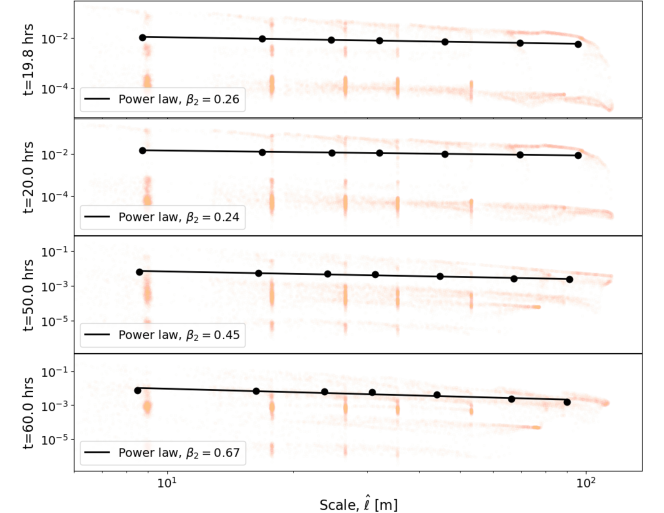
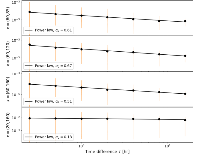
Figures 6 and 7 provide a spatio-temporal scaling analysis to further assess the heterogeneity and intermittency of dynamics in our simulation. The mean deformation rates (black dots) exhibit power law behavior (black lines), indicating the model captures localization of large strain rates in both space and in time. This is in agreement with scaling analyses of observed ice motion (see e.g., Marsan \BOthers. (\APACyear2004); Oikkonen \BOthers. (\APACyear2017)) as well as other modeling results (see e.g., Girard \BOthers. (\APACyear2009); Dansereau \BOthers. (\APACyear2016); Rampal \BOthers. (\APACyear2019)). The values of , which are larger at later times, are in agreement with the damage fields in Figure 4 and the strain rates in Figure 8. Initially the ice has relatively homogeneous strain rates, except for a few localized arching events, but the strain rates are more heterogeneous at later times when the ice has broken into many small floes. The temporal scaling coefficients are larger for points in and below the neck of the channel, which indicates strong temporal localization of strain rates in these areas. This makes intuitive sense: these regions experience a short period of high strain rates during the initial fracture event and then are in relatively free drift.
Figure 8 complements the quantitative scaling analysis with a visual representation of the principal strain rates. The velocities of the DEM particles are mapped onto a Delaunay triangulation of the particle centroids at , which allows the strain rate tensor to be computed over the cells in the triangulation. The strain rates are localized in the same regions that experience large damage rates (see Figure 4). Bands of compressive strain rates (negative values) can also be seen on either side of large tensile strain rates (positive values), indicating that the arches are supporting the ice above.
We feel the results from the idealized channel simulations show how the bonded DEM approach is able to capture the salient features of ice advecting through a constriction and the subsequent jamming, as well as important deformation characteristics (heterogeneity and intermittency) seen in real sea ice. Next, we apply this same model to the Nares Strait geometry and estimate a distribution of floe areas and the amount of ice flowing out of Kane Basin into Smith Sound.
6 Nares Strait Simulation
In our Nares Strait simulations we once again adopt the linearly-increasing wind current and stagnant ocean current used in Dansereau \BOthers. (\APACyear2017). The wind field is oriented down channel starting at 0 m/s and increasing to 22 m/s over 24 hours, which is then held constant through 72 hours. As noted by Dansereau \BOthers. (\APACyear2017), ice motion through Nares Strait is believed to be primarily driven by winds flowing south between Ellesmere Island and Greenland. The model parameters used in these simulations are similar to those in Table 1, except for the number of particles. Our model domain is a reduced region of Nares Strait focused on Kane Basin, and we use MODIS imagery from June 28, 2003 to initialize the ice extent (see section 3 and Figure 2a). We chose the June 28, 2003 ice state because the clarity of the MODIS imagery before and after the arch fails provides a useful comparison. The resultant particle set has polygonal ice particles, and stationary boundary particles. Although not shown here, we created additional particle set with more and less ice particles and found very similar results, suggesting that the particle set is able to capture the salient dynamics.
Our model uses synthetic wind and ocean loads, as well as a uniform ice thickness of 1 m, meaning the driving forces and ice conditions in the model do not precisely match the conditions in the real Nares Strait. Due to these discrepancies, we do not expect an exact match between model and observations, and therefore provide a qualitative comparison in Figure 9 as an illustration of how the bonded DEM model is a useful tool for simulating and studying ice dynamics within channel domains. Despite the aforementioned differences, there are similarities between the model and observations. Figure 9a shows a rounded fracture upstream of the initial arch, resulting from tensile failure near the right edge of the arch that propagates into the ice. This arch-like fracture is clearly seen as one of the first major break up events in the corresponding MODIS image. As the break up progresses to Figure 9b, additional fractures form upstream of these initial arch-like cracks, which is captured by the model (black boxes). The ice in the yellow boxes has begun to break up further, and a series linear of cracks have started emanating from the coastline as the ice is crushed and sheared against the land (green boxes).
At this point in the simulation there are multiple cracks bisecting the channel and long fractures along the boundaries that effectively separate the ice in the side inlets and channels from the ice in Kane Basin. After a period of time the cracks along the boundaries accumulate more damage as the ice is crushed against the coastline. Eventually the ice in the middle of the channel is no longer bonded to the boundaries and it begins to flow into Smith Sound. Similarly, we see that the observed ice also begins to move towards Smith Sound, but not uniformly. The ice moves fastest within a linear region extending from the exit of Kennedy Channel to the entrance to Smith Sound. The ice to the east of this region moves slower–particularly the ice near Humboldt Glacier. The model contains multiple cracks that separate this portion of the ice from the main channel, which is predominantly landfast. Landfast ice is also modeled in other regions, especially in the fjords, inlets, and channels off of Nares Strait, which is also observed in the simulations of Dansereau \BOthers. (\APACyear2017), the RADARSAT observations of Yackel \BOthers. (\APACyear2001), and the estimated strains in Parno \BOthers. (\APACyear2019).
The ice continues to break up as it advects out of Kane Basin (Figure 9c), and considerable break up occurs along the southern coastlines that form the constriction. The model is able to capture the ice crushing (black boxes) and breaking up into floe-like objects (green boxes) in regions similar to the MODIS imagery. Interestingly, the model also captures the formation of an open-water region (pink boxes) as the ice is sheared away from the western coastline. The ice near the exit of Kennedy channel continues to break up into many large floes (yellow boxes). Eventually the southern arch fails completely, and our model produces several floe-like objects exiting Kane Basin, which is also clearly seen in the corresponding MODIS image (light-blue boxes).
One major difference between the model and observations is that the simulation produces a stable arch where Kennedy Channel enters Kane Basin. This arch restricts ice from advecting into and “refilling” Kane basin, which results in the large open water region near the top of the basin. This is not observed in the MODIS imagery and this model-reality mismatch is likely a result of the model initial conditions and wind direction. The model starts with 100% ice concentration in Kennedy channel with ice that is also bonded to the sides of the channel. This landfast ice likely overestimates the strength of the ice in the region, creating conditions where a stable arch can form. The MODIS image in Figure 9a indicates that the ice in Kennedy Channel has clear areas of open water, and there does not appear to be significant regions of landfast ice, thus allowing more of the ice to advect into Nares Strait. In Parno \BOthers. (\APACyear2019), the ice in Nares Strait was also observed to flow in from Kennedy channel towards Humboldt Glacier. Despite there being no stable arch in the MODIS imagery, this modeled arch closely matches an arch in the Nares Strait simulation of Dansereau \BOthers. (\APACyear2017) using similar conditions (see Figure 6c 72 hour column in Dansereau \BOthers. (\APACyear2017)).
We quantify individual floes as regions of particles that are still connected to each other through cohesive beams. Varying the material cohesion parameter affects the amount of break up in the ice, which therefore affects the size distribution of the simulated floes leaving the channel. Figure 10d compares distributions of floe area from three different simulations with different cohesion ranges after 72 hours. Similar to Dansereau \BOthers. (\APACyear2017), lower cohesion results in more break up, as indicated by the larger number of small floes for lower cohesion distributions in Figure 10d. Although we are unaware of any observed floe size distributions for Nares Strait in the literature, the area distributions follow the general trend of few large floes and many small floes, which match general observations from the field (Weiss \BBA Marsan, \APACyear2004). A significant percentage of these small floes are particles whose bonds have entirely failed through crushing against the coastlines, which can be seen as the large blue regions in Figure 10a, b, and c. The size of these highly-damaged regions appear to increase in size as cohesion values decrease, which reflects weaker ice crushing more readily against boundaries than stronger ice.
Variation in how much the ice breaks apart directly affects the mass export out of Nares Strait. Figure 10e shows the normalized ice mass exiting Kane Basin into Smith Sound for the three simulations above. The results are normalized by the largest mass export at hours for the and case in order to show general trends in the simulated ice mass export for the region. We assume a uniform ice thickness, and therefore it is misleading to directly compare to the simulated ice mass to observations of ice with varying thickness. The ice in all three simulations start to leave Kane Basin at roughly the same time and same rate, however the final mass exports are significantly different, with lower cohesion values corresponding to larger mass export. The lower cohesion ice breaks into many small floes, which are able to flow out of the basin at a higher rate than the stronger ice, which remains consolidated in larger floes. These results indicate that weaker ice can lead to earlier outflow and more overall ice moving through Nares Strait, which supports the findings of Dansereau \BOthers. (\APACyear2017) and Moore \BOthers. (\APACyear2021). These results also suggest the bonded DEM could be a useful approach for studying the increase in ice export seen in recent years through Nares Strait (Moore \BOthers., \APACyear2021), particularly as increasingly realistic ice thickness, wind forcing, and other variables are incorporated into future versions of the model.
7 Discussion and Conclusions
We present a bonded DEM model that uses the cohesive beam model and a non-local Mohr-Coulomb failure approach to simulate sea ice dynamics. We use an idealized channel domain and a Nares Strait domain to illustrate how the model can deform continuous ice and subsequently fracture it into many disparate floes. Figures 3a, 3d, and 5a show how the model can simulate continuous velocities and stresses throughout the ice that account for boundary effects and stress concentrations. Figure 5b shows that once failure occurs, large tensile stresses often precede the crack tips as they propagate through the ice, which matches observations of lead formation in nature (Timco \BBA Weeks, \APACyear2010). The results in Figures 3c, 4, and 9 show how the model produces many of the salient features of ice advecting through constricted regions-namely jamming, arch-shaped fractures, and ice crushing against solid boundaries. The scaling analyses presented in Figures 6 and 7 illustrate how our bonded DEM simulations exhibit heterogeneity and intermittency in the resultant ice deformation. These metrics have been used to validate continuum sea ice models in the past, but to the best of our knowledge, have not previously been applied to DEM models of sea ice.
Section 2.2 and the work of André \BOthers. (\APACyear2013) highlight that local per-beam failure models used in previous DEM studies can fail to capture continuous fracture paths in elastic brittle materials. These methods do not consider the fracturing events occurring near each other within the ice, and therefore can exhibit fragmenting behavior. We addressed this issue with a non-local failure model that considers the stress and fractures occurring within a small region around each particle. If the particle’s stress state violates a Mohr-Coulomb criteria then the model selectively chooses which bonds to break at that instance in time, and therefore avoids the fragmenting behavior observed by André \BOthers. (\APACyear2013). In addition, our bond clipping method encourages tensile crack growth, matching observations of ice.
Comparing the Nares Strait simulation with the MODIS images in Figure 9 shows the potential for using this model to simulate real world scenarios. The model is able to qualitatively capture many of the salient features, including how the southern arch fractures into multiple large floes, and the development of multiple arch-like fractures upstream within Kane Basin. The model also accurately simulates landfast ice in the channels and fjords off of the Basin and near Humboldt Glacier, similar to the observations of Yackel \BOthers. (\APACyear2001). Figure 10 shows how the modeled ice fractures into different sized floes near the exit of Kane Basin into Smith Sound, similar to the observed ice in Figure 9a. As expected, we see a correlation between weaker ice, earlier failure of the ice arches, and increased ice export out of the strait.
The idealized channel simulations allow us to compare our DEM results with the different continuum approaches used to simulate ice advecting through similar geometries. Both Dumont \BOthers. (\APACyear2009) and Rasmussen \BOthers. (\APACyear2010) used models based on the EVP rheology, and Dumont \BOthers. (\APACyear2009) showed that it is possible to capture stable ice bridges in a channel by modifying the eccentricity of the EVP elliptical yield curve. However, Rasmussen \BOthers. (\APACyear2010) noted that due to the isotropic assumption in the EVP model, it may be unsuitable for simulating ice in Nares Strait because the complex coastline affects the ice stress state at much smaller scales than km. Alternatively, Dansereau \BOthers. (\APACyear2017) used the Maxwell elasto-brittle (Maxwell-EB) model, which tracks strain induced damage in the ice to approximate the location of leads and cracks.
Our results in Figures 3, 4, and 5 match the simulated results in Dansereau \BOthers. (\APACyear2017) remarkably well considering the differences in modeling approaches. We believe this is one of the strengths in our approach. While DEM models are known to be well-suited for MIZ simulations (Damsgaard \BOthers., \APACyear2018), where continuum sea ice methods may suffer in accuracy, we believe the results in Sections 5 and 6 also indicate that the DEM can qualitatively match the continuum-like behavior captured with the Maxwell-EB model, as well as subsequent complex fracture events, for sea ice flowing through channels. In addition, the spatial and temporal analyses indicate that the bonded DEM is able to capture important deformation properties of sea ice, like spatial heterogeneity and temporal intermittency. This suggests that DEM models have the potential to capture sea ice behavior across contiguous, fractured, and completely broken regimes. We do not attempt to definitively state when and where DEM models should be used instead of continuum models, as both approaches have utility in the sea ice modeling landscape. Instead, we aim to show that the bonded DEM approach can capture continuum-like behavior within consolidated ice, as well as the transition to highly-discontinuous ice after failure. Future work will continue to validate the model results against observations of real ice, in non-channel domains, and across a range of spatial and temporal scales.
Despite the qualitative agreement between our model results, the Dansereau \BOthers. (\APACyear2017) results, and satellite observations, there are several areas where the DEM model could be improved. First and foremost, assimilating more observational data into the model could improve accuracy. For example, we used wind speeds that approximate a large idealized storm passing through the idealized channel and Nares Strait. Actual winds were slower and more complex. As a result we see much larger displacements in that simulation than after 72 hours in the MODIS imagery. This uniform wind load and the stagnant ocean load vastly oversimplify the drag loads acting on the real ice. Incorporating more accurate wind and ocean data could improve the accuracy of the model. In addition, infusing additional data products such as SAR imagery can inform future simulations with a better understanding of the ice type (first-year or multi-year), thickness, or existing flaws, which can significantly change the ice properties. Future simulations will assimilate more data, as it’s available.
At this point our model does not evolve any thermodynamics or change the ice thickness throughout the simulation. Hibler \BOthers. (\APACyear2006) states that the Nares Strait arch may become stronger due to thermodynamic processes, which our model ignores, and could be a source of mismatch between the simulated results and observations. However, the time scales of these DEM simulations are quite short - on the order of several hours or a few days. Effects such as thermodynamic thickening likely play a smaller role in the dynamics over these short timescales. However, mechanical thickening could play an important role in these regional scale simulations, particularly in the large crushing regions in Figures 9 and 10 where the ice in Nares Strait would likely become thicker due to ridging. In fact these same regions become thicker in the Nares Strait simulations in both Dumont \BOthers. (\APACyear2009) (Figure 13) and Dansereau \BOthers. (\APACyear2017) (Figure 11a). Future DEM studies will vary ice particle thicknesses to investigate how thickness affects arch stability, and how it relates to earlier arch break up and greater export out of the strait.
A known limitation with bonded DEM or lattice spring methods is the need to calibrate local model parameters (Nguyen \BOthers., \APACyear2019). Often times setting the bond’s properties such as Young’s Modulus, or failure strengths to the macroscopic values of a particular material do not yield realistic results. The extra step of calibrating these parameters to achieve realistic elastic and fracture behavior can be time consuming, and does not guarantee accurate macroscopic behavior. Future work may incorporate an optimization routine to learn the appropriate model parameters from the mismatch between model output and satellite observations. Alternatively, the use of non-local distinct lattice spring (André \BOthers., \APACyear2019), or peridynamic models (Davis \BOthers., \APACyear2021; Silling \BBA Askari, \APACyear2005) could avoid the need for time intensive calibration studies, and facilitate using real-world values for the model parameters.
As sea ice models continue to develop towards forecasting dynamics on tactically-relevant scales, the ability to model explicit leads and cracks in the ice may prove critical to the overall utility of the ice forecasts. Future studies will look at how well the bonded DEM method presented here can capture dynamics across a range of spatial scales, including those relevant to navigation and shipping. We feel that the bonded-DEM with a non-local failure model shows promise as a useful tool to provide estimates of compression, deformation, and lead formation, thereby filling the gaps in current operational ice products identified by IICWG (\APACyear2019).
8 Open Research
Information on the ParticLS software library is included in Davis \BOthers. (\APACyear2021), and the parameters necessary to reproduce these ParticLS simulations are described in the text and in Table 1. MODIS imagery were provided by the NASA Worldview application (https://worldview.earthdata.nasa.gov/).
Acknowledgements.
We would like to thank the reviewers for their careful review and constructive feedback, which greatly improved our article. This research was funded as part of the U.S. Army Program Element 060311A, Ground Advanced Technology task for Sensing and Prediction of Arctic Maritime Coastal Conditions, through the Office of Naval Research SIDEx program, grant N000142MP001, and an Office of Naval Research MURI grant N00014-20-1-2595. We acknowledge the use of MODIS imagery provided by the NASA Worldview application (https://worldview.earthdata.nasa.gov/), part of the NASA Earth Observing System Data and Information System (EOSDIS).References
- André \BOthers. (\APACyear2019) \APACinsertmetastarAndre2019{APACrefauthors}André, D., Girardot, J.\BCBL \BBA Hubert, C. \APACrefYearMonthDay2019. \BBOQ\APACrefatitleA novel DEM approach for modeling brittle elastic media based on distinct lattice spring model A novel dem approach for modeling brittle elastic media based on distinct lattice spring model.\BBCQ \APACjournalVolNumPagesComputer Methods in Applied Mechanics and Engineering350100–122. \PrintBackRefs\CurrentBib
- André \BOthers. (\APACyear2012) \APACinsertmetastarAndre2012{APACrefauthors}André, D., Iordanoff, I., Charles, J\BHBIl.\BCBL \BBA Néauport, J. \APACrefYearMonthDay2012. \BBOQ\APACrefatitleDiscrete element method to simulate continuous material by using the cohesive beam model Discrete element method to simulate continuous material by using the cohesive beam model.\BBCQ \APACjournalVolNumPagesComputer methods in applied mechanics and engineering213113–125. \PrintBackRefs\CurrentBib
- André \BOthers. (\APACyear2013) \APACinsertmetastarAndre2013{APACrefauthors}André, D., Jebahi, M., Iordanoff, I., Charles, J\BHBIl.\BCBL \BBA Néauport, J. \APACrefYearMonthDay2013. \BBOQ\APACrefatitleUsing the discrete element method to simulate brittle fracture in the indentation of a silica glass with a blunt indenter Using the discrete element method to simulate brittle fracture in the indentation of a silica glass with a blunt indenter.\BBCQ \APACjournalVolNumPagesComputer Methods in Applied Mechanics and Engineering265136–147. \PrintBackRefs\CurrentBib
- André \BOthers. (\APACyear2017) \APACinsertmetastarAndre2017{APACrefauthors}André, D., Levraut, B., Tessier-Doyen, N.\BCBL \BBA Huger, M. \APACrefYearMonthDay2017. \BBOQ\APACrefatitleA discrete element thermo-mechanical modelling of diffuse damage induced by thermal expansion mismatch of two-phase materials A discrete element thermo-mechanical modelling of diffuse damage induced by thermal expansion mismatch of two-phase materials.\BBCQ \APACjournalVolNumPagesComputer Methods in Applied Mechanics and Engineering318898–916. \PrintBackRefs\CurrentBib
- Bouchat \BBA Tremblay (\APACyear2017) \APACinsertmetastarBouchat2017{APACrefauthors}Bouchat, A.\BCBT \BBA Tremblay, B. \APACrefYearMonthDay2017. \BBOQ\APACrefatitleUsing sea-ice deformation fields to constrain the mechanical strength parameters of geophysical sea ice Using sea-ice deformation fields to constrain the mechanical strength parameters of geophysical sea ice.\BBCQ \APACjournalVolNumPagesJournal of Geophysical Research: Oceans12275802–5825. \PrintBackRefs\CurrentBib
- Bourne \BOthers. (\APACyear2018) \APACinsertmetastarbourne2018semi{APACrefauthors}Bourne, D\BPBIP., Schmitzer, B.\BCBL \BBA Wirth, B. \APACrefYearMonthDay2018. \BBOQ\APACrefatitleSemi-discrete unbalanced optimal transport and quantization Semi-discrete unbalanced optimal transport and quantization.\BBCQ \APACjournalVolNumPagesarXiv preprint arXiv:1808.01962. \PrintBackRefs\CurrentBib
- Coon \BOthers. (\APACyear2007) \APACinsertmetastarCoon2007{APACrefauthors}Coon, M., Kwok, R., Levy, G., Pruis, M., Schreyer, H.\BCBL \BBA Sulsky, D. \APACrefYearMonthDay2007. \BBOQ\APACrefatitleArctic Ice Dynamics Joint Experiment (AIDJEX) assumptions revisited and found inadequate Arctic ice dynamics joint experiment (aidjex) assumptions revisited and found inadequate.\BBCQ \APACjournalVolNumPagesJournal of Geophysical Research: Oceans112C11. \PrintBackRefs\CurrentBib
- Damsgaard \BOthers. (\APACyear2018) \APACinsertmetastarDamsgaard2018{APACrefauthors}Damsgaard, A., Adcroft, A.\BCBL \BBA Sergienko, O. \APACrefYearMonthDay2018. \BBOQ\APACrefatitleApplication of Discrete Element Methods to Approximate Sea Ice Dynamics Application of discrete element methods to approximate sea ice dynamics.\BBCQ \APACjournalVolNumPagesJournal of Advances in Modeling Earth Systems1092228–2244. \PrintBackRefs\CurrentBib
- Dansereau \BOthers. (\APACyear2016) \APACinsertmetastarDansereau2016{APACrefauthors}Dansereau, V., Weiss, J., Saramito, P.\BCBL \BBA Lattes, P. \APACrefYearMonthDay2016. \BBOQ\APACrefatitleA Maxwell elasto-brittle rheology for sea ice modelling A maxwell elasto-brittle rheology for sea ice modelling.\BBCQ \APACjournalVolNumPagesThe Cryosphere1031339–1359. \PrintBackRefs\CurrentBib
- Dansereau \BOthers. (\APACyear2017) \APACinsertmetastarDansereau2017{APACrefauthors}Dansereau, V., Weiss, J., Saramito, P., Lattes, P.\BCBL \BBA Coche, E. \APACrefYearMonthDay2017. \BBOQ\APACrefatitleIce bridges and ridges in the Maxwell-EB sea ice rheology Ice bridges and ridges in the maxwell-eb sea ice rheology.\BBCQ \APACjournalVolNumPagesThe Cryosphere1152033. \PrintBackRefs\CurrentBib
- Davis \BOthers. (\APACyear2021) \APACinsertmetastarDavis2021{APACrefauthors}Davis, A\BPBID., West, B\BPBIA., Frisch, N\BPBIJ., O’Connor, D\BPBIT.\BCBL \BBA Parno, M\BPBID. \APACrefYearMonthDay2021. \BBOQ\APACrefatitleParticLS: Object-oriented software for discrete element methods and peridynamics Particls: Object-oriented software for discrete element methods and peridynamics.\BBCQ \APACjournalVolNumPagesComputational Particle Mechanics1–13. \PrintBackRefs\CurrentBib
- Dumont \BOthers. (\APACyear2009) \APACinsertmetastarDumont2009{APACrefauthors}Dumont, D., Gratton, Y.\BCBL \BBA Arbetter, T\BPBIE. \APACrefYearMonthDay2009. \BBOQ\APACrefatitleModeling the dynamics of the North Water polynya ice bridge Modeling the dynamics of the north water polynya ice bridge.\BBCQ \APACjournalVolNumPagesJournal of Physical Oceanography3961448–1461. \PrintBackRefs\CurrentBib
- Girard \BOthers. (\APACyear2010) \APACinsertmetastarGirard2010{APACrefauthors}Girard, L., Amitrano, D.\BCBL \BBA Weiss, J. \APACrefYearMonthDay2010. \BBOQ\APACrefatitleFailure as a critical phenomenon in a progressive damage model Failure as a critical phenomenon in a progressive damage model.\BBCQ \APACjournalVolNumPagesJournal of Statistical Mechanics: Theory and Experiment20101. {APACrefDOI} 10.1088/1742-5468/2010/01/P01013 \PrintBackRefs\CurrentBib
- Girard \BOthers. (\APACyear2011) \APACinsertmetastarGirard2011{APACrefauthors}Girard, L., Bouillon, S., Weiss, J., Amitrano, D., Fichefet, T.\BCBL \BBA Legat, V. \APACrefYearMonthDay2011. \BBOQ\APACrefatitleA new modeling framework for sea-ice mechanics based on elasto-brittle rheology A new modeling framework for sea-ice mechanics based on elasto-brittle rheology.\BBCQ \APACjournalVolNumPagesAnnals of Glaciology5257123–132. \PrintBackRefs\CurrentBib
- Girard \BOthers. (\APACyear2009) \APACinsertmetastarGirard2009{APACrefauthors}Girard, L., Weiss, J., Molines, J\BHBIM., Barnier, B.\BCBL \BBA Bouillon, S. \APACrefYearMonthDay2009. \BBOQ\APACrefatitleEvaluation of high-resolution sea ice models on the basis of statistical and scaling properties of Arctic sea ice drift and deformation Evaluation of high-resolution sea ice models on the basis of statistical and scaling properties of arctic sea ice drift and deformation.\BBCQ \APACjournalVolNumPagesJournal of Geophysical Research: Oceans114C8. \PrintBackRefs\CurrentBib
- Gladstone \BOthers. (\APACyear2001) \APACinsertmetastarGladstone2001{APACrefauthors}Gladstone, R\BPBIM., Bigg, G\BPBIR.\BCBL \BBA Nicholls, K\BPBIW. \APACrefYearMonthDay2001. \BBOQ\APACrefatitleIceberg trajectory modeling and meltwater injection in the Southern Ocean Iceberg trajectory modeling and meltwater injection in the southern ocean.\BBCQ \APACjournalVolNumPagesJournal of Geophysical Research: Oceans106C919903–19915. \PrintBackRefs\CurrentBib
- Herman (\APACyear2013\APACexlab\BCnt1) \APACinsertmetastarHerman2013a{APACrefauthors}Herman, A. \APACrefYearMonthDay2013\BCnt1. \BBOQ\APACrefatitleNumerical modeling of force and contact networks in fragmented sea ice Numerical modeling of force and contact networks in fragmented sea ice.\BBCQ \APACjournalVolNumPagesAnnals of Glaciology5462114–120. \PrintBackRefs\CurrentBib
- Herman (\APACyear2013\APACexlab\BCnt2) \APACinsertmetastarHerman2013b{APACrefauthors}Herman, A. \APACrefYearMonthDay2013\BCnt2. \BBOQ\APACrefatitleShear-jamming in two-dimensional granular materials with power-law grain-size distribution Shear-jamming in two-dimensional granular materials with power-law grain-size distribution.\BBCQ \APACjournalVolNumPagesEntropy15114802–4821. \PrintBackRefs\CurrentBib
- Herman (\APACyear2016) \APACinsertmetastarHerman2016{APACrefauthors}Herman, A. \APACrefYearMonthDay2016. \BBOQ\APACrefatitleDiscrete-Element bonded-particle Sea Ice model DESIgn, version 1.3 a–model description and implementation Discrete-element bonded-particle sea ice model design, version 1.3 a–model description and implementation.\BBCQ \APACjournalVolNumPagesGeoscientific Model Development931219–1241. \PrintBackRefs\CurrentBib
- Hibler (\APACyear1986) \APACinsertmetastarHibler1986{APACrefauthors}Hibler, W. \APACrefYearMonthDay1986. \BBOQ\APACrefatitleIce dynamics Ice dynamics.\BBCQ \BIn \APACrefbtitleThe geophysics of sea ice The geophysics of sea ice (\BPGS 577–640). \APACaddressPublisherSpringer. \PrintBackRefs\CurrentBib
- Hibler \BOthers. (\APACyear2006) \APACinsertmetastarHibler2006{APACrefauthors}Hibler, W., Hutchings, J.\BCBL \BBA Ip, C. \APACrefYearMonthDay2006. \BBOQ\APACrefatitleSea-ice arching and multiple flow states of Arctic pack ice Sea-ice arching and multiple flow states of arctic pack ice.\BBCQ \APACjournalVolNumPagesAnnals of Glaciology44339–344. \PrintBackRefs\CurrentBib
- Hibler III (\APACyear1979) \APACinsertmetastarHibler1979{APACrefauthors}Hibler III, W. \APACrefYearMonthDay1979. \BBOQ\APACrefatitleA dynamic thermodynamic sea ice model A dynamic thermodynamic sea ice model.\BBCQ \APACjournalVolNumPagesJournal of physical oceanography94815–846. \PrintBackRefs\CurrentBib
- Hopkins (\APACyear1994) \APACinsertmetastarHopkins1994{APACrefauthors}Hopkins, M\BPBIA. \APACrefYearMonthDay1994. \BBOQ\APACrefatitleOn the ridging of intact lead ice On the ridging of intact lead ice.\BBCQ \APACjournalVolNumPagesJournal of Geophysical Research: Oceans99C816351–16360. \PrintBackRefs\CurrentBib
- Hopkins (\APACyear1996) \APACinsertmetastarHopkins1996{APACrefauthors}Hopkins, M\BPBIA. \APACrefYearMonthDay1996. \BBOQ\APACrefatitleOn the mesoscale interaction of lead ice and floes On the mesoscale interaction of lead ice and floes.\BBCQ \APACjournalVolNumPagesJournal of Geophysical Research: Oceans101C818315–18326. \PrintBackRefs\CurrentBib
- Hopkins (\APACyear2004) \APACinsertmetastarHopkins2004{APACrefauthors}Hopkins, M\BPBIA. \APACrefYearMonthDay2004. \BBOQ\APACrefatitleA discrete element Lagrangian sea ice model A discrete element lagrangian sea ice model.\BBCQ \APACjournalVolNumPagesEngineering Computations212/3/4409–421. \PrintBackRefs\CurrentBib
- Hopkins \BBA Hibler (\APACyear1991) \APACinsertmetastarHopkins1991{APACrefauthors}Hopkins, M\BPBIA.\BCBT \BBA Hibler, W\BPBID. \APACrefYearMonthDay1991. \BBOQ\APACrefatitleNumerical simulations of a compact convergent system of ice floes Numerical simulations of a compact convergent system of ice floes.\BBCQ \APACjournalVolNumPagesAnnals of Glaciology1526–30. \PrintBackRefs\CurrentBib
- Hopkins \BBA Shen (\APACyear2001) \APACinsertmetastarHopkins2001{APACrefauthors}Hopkins, M\BPBIA.\BCBT \BBA Shen, H\BPBIH. \APACrefYearMonthDay2001. \BBOQ\APACrefatitleSimulation of pancake-ice dynamics in a wave field Simulation of pancake-ice dynamics in a wave field.\BBCQ \APACjournalVolNumPagesAnnals of Glaciology33355–360. \PrintBackRefs\CurrentBib
- Hopkins \BBA Thorndike (\APACyear2006) \APACinsertmetastarHopkins2006{APACrefauthors}Hopkins, M\BPBIA.\BCBT \BBA Thorndike, A\BPBIS. \APACrefYearMonthDay2006. \BBOQ\APACrefatitleFloe formation in Arctic sea ice Floe formation in arctic sea ice.\BBCQ \APACjournalVolNumPagesJournal of Geophysical Research: Oceans111C11. \PrintBackRefs\CurrentBib
- Hunke \BOthers. (\APACyear2020) \APACinsertmetastarHunke2020{APACrefauthors}Hunke, E., Allard, R., Blain, P., Blockley, E., Feltham, D., Fichefet, T.\BDBLothers \APACrefYearMonthDay2020. \BBOQ\APACrefatitleShould Sea-Ice Modeling Tools Designed for Climate Research Be Used for Short-Term Forecasting? Should sea-ice modeling tools designed for climate research be used for short-term forecasting?\BBCQ \APACjournalVolNumPagesCurrent Climate Change reports1–16. \PrintBackRefs\CurrentBib
- Hunke \BBA Dukowicz (\APACyear1997) \APACinsertmetastarHunke1997{APACrefauthors}Hunke, E.\BCBT \BBA Dukowicz, J. \APACrefYearMonthDay1997. \BBOQ\APACrefatitleAn elastic–viscous–plastic model for sea ice dynamics An elastic–viscous–plastic model for sea ice dynamics.\BBCQ \APACjournalVolNumPagesJournal of Physical Oceanography2791849–1867. \PrintBackRefs\CurrentBib
- Hutchings \BOthers. (\APACyear2011) \APACinsertmetastarHutchings2011{APACrefauthors}Hutchings, J\BPBIK., Roberts, A., Geiger, C\BPBIA.\BCBL \BBA Richter-Menge, J. \APACrefYearMonthDay2011. \BBOQ\APACrefatitleSpatial and temporal characterization of sea-ice deformation Spatial and temporal characterization of sea-ice deformation.\BBCQ \APACjournalVolNumPagesAnnals of Glaciology5257360–368. {APACrefDOI} 10.3189/172756411795931769 \PrintBackRefs\CurrentBib
- Hutter \BBA Losch (\APACyear2020) \APACinsertmetastarHutter2020{APACrefauthors}Hutter, N.\BCBT \BBA Losch, M. \APACrefYearMonthDay2020. \BBOQ\APACrefatitleFeature-based comparison of sea ice deformation in lead-permitting sea ice simulations Feature-based comparison of sea ice deformation in lead-permitting sea ice simulations.\BBCQ \APACjournalVolNumPagesThe Cryosphere14193–113. \PrintBackRefs\CurrentBib
- IICWG (\APACyear2019) \APACinsertmetastarMariner2019{APACrefauthors}IICWG. \APACrefYearMonthDay2019. \APACrefbtitleMariner Training Requirement: Intermediate report to Ice Service Heads Mariner training requirement: Intermediate report to ice service heads \APACbVolEdTR\BTR. \PrintBackRefs\CurrentBib
- Jirásek \BBA Bažant (\APACyear1995) \APACinsertmetastarJirasek1995{APACrefauthors}Jirásek, M.\BCBT \BBA Bažant, Z\BPBIP. \APACrefYearMonthDay1995. \BBOQ\APACrefatitleParticle model for quasibrittle fracture and application to sea ice Particle model for quasibrittle fracture and application to sea ice.\BBCQ \APACjournalVolNumPagesJournal of engineering mechanics12191016–1025. \PrintBackRefs\CurrentBib
- Jou \BOthers. (\APACyear2019) \APACinsertmetastarJou2019{APACrefauthors}Jou, O., Celigueta, M\BPBIA., Latorre, S., Arrufat, F.\BCBL \BBA Oñate, E. \APACrefYearMonthDay2019. \BBOQ\APACrefatitleA bonded discrete element method for modeling ship–ice interactions in broken and unbroken sea ice fields A bonded discrete element method for modeling ship–ice interactions in broken and unbroken sea ice fields.\BBCQ \APACjournalVolNumPagesComputational Particle Mechanics64739–765. \PrintBackRefs\CurrentBib
- Kawamoto \BOthers. (\APACyear2016) \APACinsertmetastarKawamoto2016{APACrefauthors}Kawamoto, R., Andò, E., Viggiani, G.\BCBL \BBA Andrade, J\BPBIE. \APACrefYearMonthDay2016. \BBOQ\APACrefatitleLevel set discrete element method for three-dimensional computations with triaxial case study Level set discrete element method for three-dimensional computations with triaxial case study.\BBCQ \APACjournalVolNumPagesJournal of the Mechanics and Physics of Solids911–13. \PrintBackRefs\CurrentBib
- Kawamoto \BOthers. (\APACyear2018) \APACinsertmetastarKawamoto2018{APACrefauthors}Kawamoto, R., Andò, E., Viggiani, G.\BCBL \BBA Andrade, J\BPBIE. \APACrefYearMonthDay2018. \BBOQ\APACrefatitleAll you need is shape: Predicting shear banding in sand with LS-DEM All you need is shape: Predicting shear banding in sand with ls-dem.\BBCQ \APACjournalVolNumPagesJournal of the Mechanics and Physics of Solids111375–392. \PrintBackRefs\CurrentBib
- Kulchitsky \BOthers. (\APACyear2017) \APACinsertmetastarKulchitsky2017{APACrefauthors}Kulchitsky, A., Hutchings, J\BPBIK., Velikhov, G., Johnson, J.\BCBL \BBA Lewis, B. \APACrefYearMonthDay2017. \APACrefbtitleSiku sea ice discrete element method model Siku sea ice discrete element method model \APACbVolEdTRFinal Report \BNUM OCS Study BOEM 2017-043. \APACaddressInstitutionBureau Ocean Energy Management. \PrintBackRefs\CurrentBib
- Kwok (\APACyear2001) \APACinsertmetastarKwok2001{APACrefauthors}Kwok, R. \APACrefYearMonthDay2001. \BBOQ\APACrefatitleDeformation of the Arctic Ocean sea ice cover between November 1996 and April 1997: a qualitative survey Deformation of the arctic ocean sea ice cover between november 1996 and april 1997: a qualitative survey.\BBCQ \BIn \APACrefbtitleIUTAM symposium on scaling laws in ice mechanics and ice dynamics Iutam symposium on scaling laws in ice mechanics and ice dynamics (\BPGS 315–322). \PrintBackRefs\CurrentBib
- Lévy \BBA Schwindt (\APACyear2018) \APACinsertmetastarlevy2018notions{APACrefauthors}Lévy, B.\BCBT \BBA Schwindt, E\BPBIL. \APACrefYearMonthDay2018. \BBOQ\APACrefatitleNotions of optimal transport theory and how to implement them on a computer Notions of optimal transport theory and how to implement them on a computer.\BBCQ \APACjournalVolNumPagesComputers & Graphics72135–148. \PrintBackRefs\CurrentBib
- Logg \BBA Wells (\APACyear2010) \APACinsertmetastardolfin2010{APACrefauthors}Logg, A.\BCBT \BBA Wells, G\BPBIN. \APACrefYearMonthDay2010apr. \BBOQ\APACrefatitleDOLFIN: Automated Finite Element Computing Dolfin: Automated finite element computing.\BBCQ \APACjournalVolNumPagesACM Trans. Math. Softw.372. {APACrefURL} https://doi.org/10.1145/1731022.1731030 {APACrefDOI} 10.1145/1731022.1731030 \PrintBackRefs\CurrentBib
- Løset (\APACyear1994\APACexlab\BCnt1) \APACinsertmetastarLoset1994_Pt2{APACrefauthors}Løset, S. \APACrefYearMonthDay1994\BCnt1. \BBOQ\APACrefatitleDiscrete element modelling of a broken ice field-Part II: simulation of ice loads on a boom Discrete element modelling of a broken ice field-part ii: simulation of ice loads on a boom.\BBCQ \APACjournalVolNumPagesCold regions science and technology224349–360. \PrintBackRefs\CurrentBib
- Løset (\APACyear1994\APACexlab\BCnt2) \APACinsertmetastarLoset1994_Pt1{APACrefauthors}Løset, S. \APACrefYearMonthDay1994\BCnt2. \BBOQ\APACrefatitleDiscrete element modelling of a broken ice field-Part I: model development Discrete element modelling of a broken ice field-part i: model development.\BBCQ \APACjournalVolNumPagesCold regions science and technology224339–347. \PrintBackRefs\CurrentBib
- Marsan \BOthers. (\APACyear2004) \APACinsertmetastarMarsan2004{APACrefauthors}Marsan, D., Stern, H., Lindsay, R.\BCBL \BBA Weiss, J. \APACrefYearMonthDay2004. \BBOQ\APACrefatitleScale dependence and localization of the deformation of arctic sea ice Scale dependence and localization of the deformation of arctic sea ice.\BBCQ \APACjournalVolNumPagesPhysical Review Letters9317. \PrintBackRefs\CurrentBib
- Martin \BBA Adcroft (\APACyear2010) \APACinsertmetastarMartin2010{APACrefauthors}Martin, T.\BCBT \BBA Adcroft, A. \APACrefYearMonthDay2010. \BBOQ\APACrefatitleParameterizing the fresh-water flux from land ice to ocean with interactive icebergs in a coupled climate model Parameterizing the fresh-water flux from land ice to ocean with interactive icebergs in a coupled climate model.\BBCQ \APACjournalVolNumPagesOcean Modelling343-4111–124. \PrintBackRefs\CurrentBib
- Moore \BOthers. (\APACyear2021) \APACinsertmetastarMoore2021{APACrefauthors}Moore, G., Howell, S., Brady, M., Xu, X.\BCBL \BBA McNeil, K. \APACrefYearMonthDay2021. \BBOQ\APACrefatitleAnomalous collapses of Nares Strait ice arches leads to enhanced export of Arctic sea ice Anomalous collapses of nares strait ice arches leads to enhanced export of arctic sea ice.\BBCQ \APACjournalVolNumPagesNature Communications1211–8. \PrintBackRefs\CurrentBib
- Nguyen \BOthers. (\APACyear2019) \APACinsertmetastarNguyen2019{APACrefauthors}Nguyen, T\BHBIT., André, D.\BCBL \BBA Huger, M. \APACrefYearMonthDay2019. \BBOQ\APACrefatitleAnalytic laws for direct calibration of discrete element modeling of brittle elastic media using cohesive beam model Analytic laws for direct calibration of discrete element modeling of brittle elastic media using cohesive beam model.\BBCQ \APACjournalVolNumPagesComputational Particle Mechanics63393–409. \PrintBackRefs\CurrentBib
- Oikkonen \BOthers. (\APACyear2017) \APACinsertmetastarOikkonen2017{APACrefauthors}Oikkonen, A., Happala, J., Lensu, M., Karvonen, J.\BCBL \BBA Itkin, P. \APACrefYearMonthDay2017. \BBOQ\APACrefatitleSmall-scale sea ice deformation during N-ICE2015: From compact pack ice to marginal ice zone Small-scale sea ice deformation during N-ICE2015: From compact pack ice to marginal ice zone.\BBCQ \APACjournalVolNumPagesJournal of Geophysical Research: Oceans1225105–5120. {APACrefDOI} 10.1002/2016JC012387 \PrintBackRefs\CurrentBib
- Otsu (\APACyear1979) \APACinsertmetastarOtsu1979{APACrefauthors}Otsu, N. \APACrefYearMonthDay1979. \BBOQ\APACrefatitleA threshold selection method from gray-level histograms A threshold selection method from gray-level histograms.\BBCQ \APACjournalVolNumPagesIEEE transactions on systems, man, and cybernetics9162–66. \PrintBackRefs\CurrentBib
- Parno \BOthers. (\APACyear2019) \APACinsertmetastarParno2019{APACrefauthors}Parno, M\BPBID., West, B\BPBIA., Song, A\BPBIJ., Hodgdon, T\BPBIS.\BCBL \BBA O’Connor, D. \APACrefYearMonthDay2019. \BBOQ\APACrefatitleRemote measurement of sea ice dynamics with regularized optimal transport Remote measurement of sea ice dynamics with regularized optimal transport.\BBCQ \APACjournalVolNumPagesGeophysical Research Letters46105341–5350. \PrintBackRefs\CurrentBib
- Rallabandi \BOthers. (\APACyear2017) \APACinsertmetastarRallabandi2017{APACrefauthors}Rallabandi, B., Zheng, Z., Winton, M.\BCBL \BBA Stone, H\BPBIA. \APACrefYearMonthDay2017. \BBOQ\APACrefatitleFormation of sea ice bridges in narrow straits in response to wind and water stresses Formation of sea ice bridges in narrow straits in response to wind and water stresses.\BBCQ \APACjournalVolNumPagesJournal of Geophysical Research: Oceans12275588–5610. \PrintBackRefs\CurrentBib
- Rampal \BOthers. (\APACyear2016) \APACinsertmetastarRampal2016{APACrefauthors}Rampal, P., Bouillon, S., Ólason, E.\BCBL \BBA Morlighem, M. \APACrefYearMonthDay2016. \BBOQ\APACrefatitleneXtSIM: a new Lagrangian sea ice model nextsim: a new lagrangian sea ice model.\BBCQ \APACjournalVolNumPagesThe Cryosphere1031055–1073. \PrintBackRefs\CurrentBib
- Rampal \BOthers. (\APACyear2019) \APACinsertmetastarRampal2019{APACrefauthors}Rampal, P., Dansereau, V., Olason, E., Bouillon, S., Williams, T., Korosov, A.\BCBL \BBA Samaké, A. \APACrefYearMonthDay2019. \BBOQ\APACrefatitleOn the multi-fractal scaling properties of sea ice deformation On the multi-fractal scaling properties of sea ice deformation.\BBCQ \APACjournalVolNumPagesCryosphere1392457–2474. {APACrefDOI} 10.5194/tc-13-2457-2019 \PrintBackRefs\CurrentBib
- Rampal \BOthers. (\APACyear2008) \APACinsertmetastarRampal2008{APACrefauthors}Rampal, P., Weiss, J., Marsan, D., Lindsay, R.\BCBL \BBA Stern, H. \APACrefYearMonthDay2008. \BBOQ\APACrefatitleScaling properties of sea ice deformation from buoy dispersion analysis Scaling properties of sea ice deformation from buoy dispersion analysis.\BBCQ \APACjournalVolNumPagesJournal of Geophysical Research: Oceans11331–12. {APACrefDOI} 10.1029/2007JC004143 \PrintBackRefs\CurrentBib
- Rasmussen \BOthers. (\APACyear2010) \APACinsertmetastarRasmussen2010{APACrefauthors}Rasmussen, T\BPBIA., Kliem, N.\BCBL \BBA Kaas, E. \APACrefYearMonthDay2010. \BBOQ\APACrefatitleModelling the sea ice in the Nares Strait Modelling the sea ice in the nares strait.\BBCQ \APACjournalVolNumPagesOcean Modelling353161–172. \PrintBackRefs\CurrentBib
- Ringeisen \BOthers. (\APACyear2019) \APACinsertmetastarringeisen2019simulating{APACrefauthors}Ringeisen, D., Losch, M., Tremblay, L\BPBIB.\BCBL \BBA Hutter, N. \APACrefYearMonthDay2019. \BBOQ\APACrefatitleSimulating intersection angles between conjugate faults in sea ice with different viscous–plastic rheologies Simulating intersection angles between conjugate faults in sea ice with different viscous–plastic rheologies.\BBCQ \APACjournalVolNumPagesThe Cryosphere1341167–1186. \PrintBackRefs\CurrentBib
- Schreyer \BOthers. (\APACyear2006) \APACinsertmetastarSchreyer2006{APACrefauthors}Schreyer, H., Sulsky, D., Munday, L., Coon, M.\BCBL \BBA Kwok, R. \APACrefYearMonthDay2006. \BBOQ\APACrefatitleElastic-decohesive constitutive model for sea ice Elastic-decohesive constitutive model for sea ice.\BBCQ \APACjournalVolNumPagesJournal of Geophysical Research: Oceans111C11. \PrintBackRefs\CurrentBib
- Schulson (\APACyear2004) \APACinsertmetastarschulson2004compressive{APACrefauthors}Schulson, E\BPBIM. \APACrefYearMonthDay2004. \BBOQ\APACrefatitleCompressive shear faults within arctic sea ice: Fracture on scales large and small Compressive shear faults within arctic sea ice: Fracture on scales large and small.\BBCQ \APACjournalVolNumPagesJournal of Geophysical Research: Oceans109C7. \PrintBackRefs\CurrentBib
- Silling \BBA Askari (\APACyear2005) \APACinsertmetastarSilling2005{APACrefauthors}Silling, S\BPBIA.\BCBT \BBA Askari, E. \APACrefYearMonthDay2005. \BBOQ\APACrefatitleA meshfree method based on the peridynamic model of solid mechanics A meshfree method based on the peridynamic model of solid mechanics.\BBCQ \APACjournalVolNumPagesComputers & structures8317-181526–1535. \PrintBackRefs\CurrentBib
- Steele \BOthers. (\APACyear1997) \APACinsertmetastarSteele1997{APACrefauthors}Steele, M., Zhang, J., Rothrock, D.\BCBL \BBA Stern, H. \APACrefYearMonthDay1997. \BBOQ\APACrefatitleThe force balance of sea ice in a numerical model of the Arctic Ocean The force balance of sea ice in a numerical model of the arctic ocean.\BBCQ \APACjournalVolNumPagesJournal of Geophysical Research: Oceans102C921061–21079. \PrintBackRefs\CurrentBib
- Sulsky \BOthers. (\APACyear2007) \APACinsertmetastarSulsky2007{APACrefauthors}Sulsky, D., Schreyer, H., Peterson, K., Kwok, R.\BCBL \BBA Coon, M. \APACrefYearMonthDay2007. \BBOQ\APACrefatitleUsing the material-point method to model sea ice dynamics Using the material-point method to model sea ice dynamics.\BBCQ \APACjournalVolNumPagesJournal of Geophysical Research: Oceans112C2. \PrintBackRefs\CurrentBib
- Sun \BBA Shen (\APACyear2012) \APACinsertmetastarSun2012{APACrefauthors}Sun, S.\BCBT \BBA Shen, H\BPBIH. \APACrefYearMonthDay2012. \BBOQ\APACrefatitleSimulation of pancake ice load on a circular cylinder in a wave and current field Simulation of pancake ice load on a circular cylinder in a wave and current field.\BBCQ \APACjournalVolNumPagesCold Regions Science and Technology7831–39. \PrintBackRefs\CurrentBib
- Thorndike \BBA Colony (\APACyear1982) \APACinsertmetastarThorndike1982{APACrefauthors}Thorndike, A.\BCBT \BBA Colony, R. \APACrefYearMonthDay1982. \BBOQ\APACrefatitleSea ice motion in response to geostrophic winds Sea ice motion in response to geostrophic winds.\BBCQ \APACjournalVolNumPagesJournal of Geophysical Research: Oceans87C85845–5852. \PrintBackRefs\CurrentBib
- Timco \BBA Weeks (\APACyear2010) \APACinsertmetastarTimco2010{APACrefauthors}Timco, G.\BCBT \BBA Weeks, W. \APACrefYearMonthDay2010. \BBOQ\APACrefatitleA review of the engineering properties of sea ice A review of the engineering properties of sea ice.\BBCQ \APACjournalVolNumPagesCold regions science and technology602107–129. \PrintBackRefs\CurrentBib
- Wadhams (\APACyear2000) \APACinsertmetastarWadhams2000{APACrefauthors}Wadhams, P. \APACrefYear2000. \APACrefbtitleIce in the Ocean Ice in the ocean. \APACaddressPublisherCRC Press. \PrintBackRefs\CurrentBib
- Weiss \BBA Dansereau (\APACyear2017) \APACinsertmetastarWeiss2017{APACrefauthors}Weiss, J.\BCBT \BBA Dansereau, V. \APACrefYearMonthDay2017. \BBOQ\APACrefatitleLinking scales in sea ice mechanics Linking scales in sea ice mechanics.\BBCQ \APACjournalVolNumPagesPhilosophical Transactions of the Royal Society A: Mathematical, Physical and Engineering Sciences375208620150352. \PrintBackRefs\CurrentBib
- Weiss \BBA Marsan (\APACyear2004) \APACinsertmetastarWeiss2004{APACrefauthors}Weiss, J.\BCBT \BBA Marsan, D. \APACrefYearMonthDay2004. \BBOQ\APACrefatitleScale properties of sea ice deformation and fracturing Scale properties of sea ice deformation and fracturing.\BBCQ \APACjournalVolNumPagesComptes Rendus Physique57735–751. \PrintBackRefs\CurrentBib
- Weiss \BOthers. (\APACyear2009) \APACinsertmetastarWeiss2009b{APACrefauthors}Weiss, J., Marsan, D.\BCBL \BBA Rampal, P. \APACrefYearMonthDay2009. \BBOQ\APACrefatitleSpace and Time Scaling Laws Induced by the Multiscale Fracturing of The Arctic Sea Ice Cover Space and Time Scaling Laws Induced by the Multiscale Fracturing of The Arctic Sea Ice Cover.\BBCQ \APACjournalVolNumPagesIUTAM Bookseries10101–109. {APACrefDOI} 10.1007/978-1-4020-9033-2_10 \PrintBackRefs\CurrentBib
- Weiss \BBA Schulson (\APACyear2009) \APACinsertmetastarWeiss2009a{APACrefauthors}Weiss, J.\BCBT \BBA Schulson, E\BPBIM. \APACrefYearMonthDay2009. \BBOQ\APACrefatitleCoulombic faulting from the grain scale to the geophysical scale: lessons from ice Coulombic faulting from the grain scale to the geophysical scale: lessons from ice.\BBCQ \APACjournalVolNumPagesJournal of Physics D: Applied Physics4221214017. \PrintBackRefs\CurrentBib
- Weiss \BOthers. (\APACyear2007) \APACinsertmetastarWeiss2007{APACrefauthors}Weiss, J., Schulson, E\BPBIM.\BCBL \BBA Stern, H\BPBIL. \APACrefYearMonthDay2007. \BBOQ\APACrefatitleSea ice rheology from in-situ, satellite and laboratory observations: Fracture and friction Sea ice rheology from in-situ, satellite and laboratory observations: Fracture and friction.\BBCQ \APACjournalVolNumPagesEarth and Planetary Science Letters2551-21–8. \PrintBackRefs\CurrentBib
- Wilchinsky \BBA Feltham (\APACyear2006) \APACinsertmetastarWilchinsky2006{APACrefauthors}Wilchinsky, A\BPBIV.\BCBT \BBA Feltham, D\BPBIL. \APACrefYearMonthDay2006. \BBOQ\APACrefatitleModelling the rheology of sea ice as a collection of diamond-shaped floes Modelling the rheology of sea ice as a collection of diamond-shaped floes.\BBCQ \APACjournalVolNumPagesJournal of non-newtonian fluid mechanics138122–32. \PrintBackRefs\CurrentBib
- Wilchinsky \BOthers. (\APACyear2010) \APACinsertmetastarWilchinsky2010{APACrefauthors}Wilchinsky, A\BPBIV., Feltham, D\BPBIL.\BCBL \BBA Hopkins, M\BPBIA. \APACrefYearMonthDay2010. \BBOQ\APACrefatitleEffect of shear rupture on aggregate scale formation in sea ice Effect of shear rupture on aggregate scale formation in sea ice.\BBCQ \APACjournalVolNumPagesJournal of Geophysical Research: Oceans115C10. \PrintBackRefs\CurrentBib
- Xin \BOthers. (\APACyear2016) \APACinsertmetastarxin2016centroidal{APACrefauthors}Xin, S\BHBIQ., Lévy, B., Chen, Z., Chu, L., Yu, Y., Tu, C.\BCBL \BBA Wang, W. \APACrefYearMonthDay2016. \BBOQ\APACrefatitleCentroidal power diagrams with capacity constraints: Computation, applications, and extension Centroidal power diagrams with capacity constraints: Computation, applications, and extension.\BBCQ \APACjournalVolNumPagesACM Transactions on Graphics (TOG)3561–12. \PrintBackRefs\CurrentBib
- Yackel \BOthers. (\APACyear2001) \APACinsertmetastarYackel2001{APACrefauthors}Yackel, J., Barber, D.\BCBL \BBA Papakyriakou, T. \APACrefYearMonthDay2001. \BBOQ\APACrefatitleOn the estimation of spring melt in the North Water polynya using RADARSAT-1 On the estimation of spring melt in the north water polynya using radarsat-1.\BBCQ \APACjournalVolNumPagesAtmosphere-Ocean393195–208. \PrintBackRefs\CurrentBib
Appendix A Details of Scaling Analysis.
A.1 Mathematical Formulation.
Consider a strain rate tensor that varies with spatial location and time . This tensor could be derived from observations of sea ice velocities or from the output of a sea ice model. Scaling analyses consider spatio-temporal averages of this pointwise strain tensor, where the average is taken over spatial subdomains defined by a length scale and time intervals defined by a timescale . Mathematically, the average strain rate tensor is given by
| (13) |
where and denote the area of and length of , respectively. From this average strain rate tensor, the total deformation rate can be computed as
| (14) |
where and are the divergent and shear components of the average strain rate, defined as
| (15) | ||||
Notice that the total deformation rate is a function of position and time but also has a dependence on the length scale and timescale .
The relationship of with scales and provides insight into the structure of the deformation field. Many studies have observed that, when averaged over all positions , the total deformation rate has a power law relationship with (e.g., Marsan \BOthers. (\APACyear2004); Hutchings \BOthers. (\APACyear2011)), so that
| (16) |
where denotes the spatial average and and are condition-specific parameters that also depend on timescale . Similar power law relationships have been observed with the timescale , resulting in relationships of the form
| (17) |
for coefficients and that depend on spatial scale . Importantly, the value of is a quantitative measure of heterogeneity in the deformation field. Similarly, is a measure of intermittency. As detailed in Girard \BOthers. (\APACyear2009), model predictions should have deformation fields that exhibit this power law behavior and have coefficients and within realistic bounds. Notice that still depends on time and still depends on space; we therefore compute at multiple times and at multiple locations.
A.2 Numerical Approximation.
In practice, we do not have access to a continuous strain rate field because of limited observations and model discretizations. To enable computation, we therefore need to approximate both the strain rate tensor itself and subsequently the integral in (13). Girard \BOthers. (\APACyear2010) employs what amounts to a piecewise constant approximation of on a regular model grid and then approximates (13) over a square domain by finding cells with centroids in and then computing an area-weighted average of the strain rates in these fields.111The authors of Girard \BOthers. (\APACyear2010) actually compute an average of the spatial gradient of the velocity field, but because the relationship between velocity gradient and strain rate is linear, this is equivalent to averaging the strain rate. Because the area of the cells will in general not be exactly, the square root of the summed cell areas is used as the “observed” length scale when computing the power law parameters. Another approach based on Delaunay triangulations of “tracer points” is used for representing and for approximating (13) in Oikkonen \BOthers. (\APACyear2017) and Rampal \BOthers. (\APACyear2019). Again, the strain rate is piecewise constant, but over triangles in the Delaunay triangulation. In that work, the averaging window is implicitly defined by subsampling the tracer points and creating triangulations with larger cells. We employ a similar triangular representation of the strain rate tensor but use an explicit spatial average of the strain rate tensor more akin to Girard \BOthers. (\APACyear2010).
A DEM simulation gives the position and velocity of each particle at a finite number of times. For the spatial scaling analysis, we use and use the instantaneous particle velocities to compute the strain rate without evaluating the temporal integral in (13). To approximate , we construct a Delaunay triangulation of the particle centroids, which gives us a triangular mesh with particle velocities corresponding to nodal velocities in this mesh. As in Oikkonen \BOthers. (\APACyear2017), we remove cells in the Delaunay triangulation with a minimum angle of less than , which could result in poor strain rate approximations and are typically found between particles that are not in contact (i.e., over open water). We also ignore cells based on boundary particles, which do not move in our simulations. Using the nodal velocities, we can then compute cell-wise strain rate tensors using standard finite element machinery (see e.g., Logg \BBA Wells (\APACyear2010)).
Let denote the centroid of cell in the triangular mesh. To compute the total deformation rate at this point, we use use a circular subdomain to define the spatial average, as opposed to the square subdomain employed in Girard \BOthers. (\APACyear2010). The circular subdomain allows us to use KD trees for efficient neighborhood searches. We find all cells in the mesh with centroids and compute the cell area-weighted average of the strain rates in these cells. More specifically,
| (18) |
where is the area of triangle in the Delaunay triangulation and is the sum of cell areas for cells intersecting . The length scale associated with this total deformation is given by . From , we can then compute the total deformation rate using (14).
For any length scale and time , we obtain pairs for each cell in the Delaunay triangulation. We use the average of these pairs (over all cells) as an estimate of in (16). The process is repeated for multiple length scales ( for our synthetic results) and a least squares fit in log-log space is used to obtain the coefficients and in the power law.
The temporal scaling analysis is simpler because the integral over time in (13) can be estimated as
| (19) |
where is a continuous displacement field that we estimate by treating the particle positions as nodal values with piecewise linear finite elements. We assume that the length scale , so we can look at cell-wise deformations and do not need to include the spatial averaging in our temporal scaling analysis. To compute the average strain rates, we construct a mesh using the positions at time , then use the change in particle positions to define nodal values for and again use standard finite element machinery to compute piecewise constant strain rate tensors in each cell of the mesh (i.e., the right hand side of (19)). For any cell, the same least squares approach described above for computing and can then be used to compute the temporal power law parameters and for in that cell.