Mosco convergence of gradient forms with
non-convex interaction potential

Abstract.

Convexity of interaction potentials is a typical condition for the derivation of gradient bounds for diffusion semigroups in stochastic interface models, particle systems, etc. Gradient bounds are often used to show convergence of semigroups. However for a large class of convergence problems the assumption of convexity fails. The article suggests a way to overcome this hindrance, as it presents a new approach which is not based on gradient bounds. Combining the theory of Dirichlet forms with methods from numerical analysis we find abstract criteria for Mosco convergence of standard gradient forms with varying reference measures. These include cases in which the measures are not log-concave. To demonstrate the accessibility of our abstract theory we discuss a first application, generalizing an approximation result from [7], which first appeared in 2011.

1. Introduction

The abstract framework presented by Kazuhiro Kuwae and Takashi Shioya in [17] takes up the functional analytic ideas of Umberto Mosco, who in [21] investigates the convergence of spectral structures on a Hilbert space, and fits it into a setting of varying Hilbert spaces. Their method has found application in partial differential equations, see e.g. [18], and in probability theory, see e.g. [7, 13, 4]. The probabilistic disputes are often motivated by problems from statistical mechanics involving the scaling limit of a dynamical system. There, one typically starts by looking at a statistically distributed ensemble of interacting particles or sites in a finite volume. Sites are the interacting entities, which replace the physical particles, in phenomenological or effective models. Technically, a finite volume marks a subset $E_{N}$ in the collection of all states $E$, which is characterized by a limited number of degrees of freedom. That number increases as the index $N\in\mathbb{N}$ increases. Descriptively, the limit of $N\to\infty$ represents a transition from a micro- or mesoscopic understanding of the problem to a macroscopic point of view. On $E_{N}$ a natural reference measure is provided by the Lebesgue measure. At each point there is a natural tangent space which isomorphic to the Euclidean space. A probability $\mu_{N}$ with a density proportional to $\exp(-V_{N})$ describes a system in its thermal equilibrium. The function $V_{N}:E_{N}\to\mathbb{R}$ is called potential, or Hamiltonian, assigned to a microscopic state. Once the weak measure convergence of $\mu_{N}$ for $N\to\infty$ is known, the closest question related to a dynamical result is concerned with the fluctuations around the equilibrium. For each $N$ such a dynamic should admit $\mu_{N}$ as a reversible measure and heuristically behave according to the stochastic differential equation

$$\mathop{}\!\mathrm{d}X_{t}=-\nabla V_{N}\mathop{}\!\mathrm{d}t+\sqrt{2}\,\mathop{}\!\mathrm{d}W_{t}.$$

Convergence of the finite-dimensional distributions of the laws on $E$ under the scaling limit $N\to\infty$ is equivalent to the Mosco convergence of the gradient-type Dirichlet forms

$$\mathcal{E}^{N}(u,v)\,=\,\int\limits_{E_{N}}{\langle\nabla u,\nabla v\rangle}_{E_{N}}\mathop{}\!\mathrm{d}\mu_{N},\qquad u,v\in\mathcal{D}(\mathcal{E}^{N}).$$ (1.1)

The elements of $\mathcal{D}(\mathcal{E}^{N})$ are contained in a local Sobolev space $H^{1,1}_{\textnormal{loc}}$ over $E_{N}$. The problem becomes more involved the less regularity is assumed for $V_{N}$. The applications we consider, do not require the continuity $V_{N}$, for example. Given the weak convergence of the invariant measures, the asymptotic analysis of the corresponding Dirichlet forms becomes an interesting topic on its own right, as it stands at the beginning of a further discussion on the probabilistic side. Gradient forms appear as standard examples in the books of [19, 12]. If the state space $E$ is Polish and $m$ is a probability measure on its Borel $\sigma$-algebra $\mathcal{B}(E)$, then the family of local, quasi-regular, conservative and symmetric Dirichlet forms on $L^{2}(E,m)$ are in 1:1 correspondence with the family of conservative $m$ -symmetric diffusion processes on $(E,\mathcal{B}(E))$ (up to equivalence). A conservative diffusion process $X=(\Omega,\mathscr{F},{(X_{t})}_{t\geq 0},{(P_{x})_{x\in E}})$ is a Hunt process with path space $C([0,\infty),E)$. The transition function $p_{t}(x,A):=P_{x}(\{X_{t}\in A\})$, $x\in E$, $A\in\mathcal{B}(E)$, $t\geq 0$, is $m$ -symmetric and hence $m$ is an invariant measure. Extending the linear operator

$$\tilde{p}_{t}:u\,\mapsto\,\int\limits_{E}u(y)\mathop{}\!\mathrm{d}p_{t}(\cdot,\mathop{}\!\mathrm{d}y),$$

which acts on the bounded, measurable functions on $E$, to a symmetric contraction operator $T_{t}$ on $L^{2}(E,m)$ for $t\geq 0$, the relation of $X$ and $\mathcal{E}$ is given by the equations

$$\mathcal{D}(\mathcal{E})\,=\,\Big{\{}\,u\in L^{2}(E,m)\,\Big{|}\,\sup_{t>0}\,\frac{1}{t}\int\limits_{E}u\,(T_{t}u-u)\mathop{}\!\mathrm{d}m\,<\infty\,\Big{\}}$$

$$\textnormal{and}\quad\mathcal{E}(u,v)\,=\,\lim_{t\to 0}\,\frac{1}{t}\int\limits_{E}u\,(T_{t}v-v)\mathop{}\!\mathrm{d}m.$$

The family ${(T_{t})}_{t\geq 0}$ forms a strongly continuous contraction semigroup on $L^{2}(E,m)$. Given a family of diffusion processes $\{$ $X^{N}=(\Omega_{N}$, $\mathscr{F}^{N}$, ${(X^{N}_{t})}_{t\geq 0}$, ${(P^{N}_{x})}_{x\in E})$, $X=(\Omega$, $\mathscr{F}$, ${(X_{t})}_{t\geq 0}$, ${(P_{x})}_{x\in E})$ $\}$, where $X^{N}$ is $m_{N}$ -symmetric and $X$ is $m$ -symmetric, we now write $\widetilde{P}_{N}(B):=\int_{E}P^{N}_{x}(B)\mathop{}\!\mathrm{d}m_{N}(x)$ for $B\in\mathscr{F}$ and $\widetilde{P}(B):=\int_{E}P_{x}(B)\mathop{}\!\mathrm{d}m(x)$ for $B\in\mathscr{F}^{N}$, $N\in\mathbb{N}$. Convergence of the finite-dimensional distributions of equilibrium fluctuations, which reads

$$\lim_{N\to\infty}\,\int\limits_{\Omega_{N}}f_{1}(X^{N}_{t_{1}})\cdot f_{2}(X^{N}_{t_{1}+t_{2}})\cdot\dots\cdot f_{k}(X^{N}_{t_{1}+t_{2}+\dots+t_{k}})\mathop{}\!\mathrm{d}\widetilde{P}_{N}\\ \begin{aligned} &=\,\lim_{N\to\infty}\,\int\limits_{E}T_{t_{1}}^{N}(f_{1}\cdot T_{t_{2}}^{N}(\dots T_{t_{k-1}}^{N}(f_{k-1}\cdot T^{N}_{t_{k}}f_{k})\dots))\mathop{}\!\mathrm{d}m_{N}(x)\\ &=\,\int\limits_{E}T_{t_{1}}(f_{1}\cdot T_{t_{2}}(\dots T_{t_{k-1}}(f_{k-1}\cdot T_{t_{k}}f_{k})\dots))\mathop{}\!\mathrm{d}m(x)\end{aligned}\\ =\,\int\limits_{\Omega_{N}}f_{1}(X_{t_{1}})\cdot f_{2}(X_{t_{1}+t_{2}})\cdot\dots\cdot f_{k}(X_{t_{1}+t_{2}+\dots+t_{k}})\mathop{}\!\mathrm{d}\widetilde{P}$$

with $f_{1},\dots,f_{k}\in C_{\textnormal{b}}(E)$, $t_{1},\dots,t_{k}\in[0,\infty)$, $k\in\mathbb{N}$, is equivalent to Mosco convergence of the corresponding sequence of Dirichlet forms towards the corresponding asymptotic form. This is due to the theorem of Mosco-Kuwae-Shioya, as stated in [17, Theorem 2.4]. Mosco convergence is formulated in terms of two conditions, (a) of [21, Definition 2.1] respectively (F1’) of [17, Definition 2.11]), and (b) of [21, Definition 2.1] respectively (F2) of [17, Definition 2.11]). In this text we call them (M1) and (M2).

The exact domain of the asymptotic form plays a crucial role. Identifying a Mosco limit includes making a statement concerning the scope of its domain. This is reflected in the contrasting interplay between the two conditions when they are looked at independently. If the sequence ${(\mathcal{E}^{N})}_{N}$ satisfies (M1) w.r.t. the asymptotic form $\mathcal{E}^{*}$ and simultaneously satisfies (M2) w.r.t. another asymptotic form $\mathcal{E}^{**}$, then $\mathcal{D}(\mathcal{E}^{**})\subseteq\mathcal{D}(\mathcal{E}^{*})$ and the quadratic form of $\mathcal{E}^{*}$ is dominated by that of $\mathcal{E}^{**}$, i.e. $\mathcal{E}^{*}(u,u)\leq\mathcal{E}^{**}(u,u)$ for $u\in\mathcal{D}(\mathcal{E}^{**})$. To show Mosco convergence we thus have to see why the ‘smallest’ asymptotic form for which (M2) holds and the ‘biggest’ asymptotic form for which (M1) holds coincide.

Even in the comfortable case, in which $E$ is a Hilbert space and the limit $\mu$ of ${(\mu_{N})}_{N}$ admits a density w.r.t. a Gaussian measure, the task of proving Mosco convergence for gradient-type forms can be challenging, depending on the nature of the density. In [7], Said Karim Bounebache and Lorenzo Zambotti investigate the instance, where $E=L^{2}((0,1),\mathop{}\!\mathrm{d}t)$ and $E_{N}$ is the linear span of indicator functions $\mathbb{1}_{[2^{-N}(i-1),2^{-N}i)}$, $i=1,\dots,2^{N}$. They show Mosco convergence for the sequence of gradient forms ${(\mathcal{E}^{N})}_{N}$, defined as in 1.1. The respective reference measure is chosen as

$$\mathop{}\!\mathrm{d}\mu_{N}(h)\,\propto\,\exp(-V(h))\,\mathop{}\!\mathrm{d}\tilde{\mu}_{N}(h),\qquad V:E\ni h\,\mapsto\,\int\limits_{0}^{1}f(h(t))\mathop{}\!\mathrm{d}t,$$ (1.2)

where $f:\mathbb{R}\to\mathbb{R}$ is of bounded variation and $\tilde{\mu}_{N}$ denotes the image measure under the orthogonal projection $E\to E_{N}$ of the law $\tilde{\mu}$ of a Brownian bridge between $0$ and $0$ in the interval $[0,1]$. The difficulty, as the authors point out, lies in the fact that measure of 1.2 is not log-concave, due to the non-convexity of the perturbing potential. The asymptotic form is a perturbed version of the standard gradient form on $E$ in the Gaussian case:

$$\mathcal{E}(u,v)\,=\,\int\limits_{E}{\langle\nabla u,\nabla v\rangle}_{E}\,\exp(-V)/Z\,\mathop{}\!\mathrm{d}\tilde{\mu},\ \quad u,v\in\mathcal{D}(\mathcal{E}).$$ (1.3)

The domain of $\mathcal{E}$ coincides with the Sobolev space $H^{1,2}(E,\tilde{\mu})$ and $Z:=\int\exp(-V)\mathop{}\!\mathrm{d}\tilde{\mu}$. The essential ingredients, which are used in the proof of [7, Thm. 5.6], are the compactness of the embedding $H^{1,2}(E,\tilde{\mu})\hookrightarrow L^{2}(E,\tilde{\mu})$ and integration by parts.

Integration by parts formulae for the invariant measures have played the key role in the proof for convergence of the equilibrium fluctuations in some relevant works such as [13] and [30]. Investigating integration by parts alone, however, is not sufficient to derive a statement for the corresponding diffusion processes. A completive concept, which is linked to the convergence of Dirichlet forms, takes the perspective of semigroups. Gradient bounds for semigroups are apt to yield a compactness result. Such can be obtained either probabilistically (see e.g. [22, 9]) or analytically (see e.g. [5, 2]). Gradient bounds have been used to prove convergence of diffusion processes in [30] (in combination with integration by parts formulae) or in [3]. However, the typical requirement for the convexity of the potential $V$, i.e. positivity of the Hessian $\nabla\nabla V$, unites the different approaches to gradient bounds and drastically restricts their applicability.

This article endeavours to find new methods and tools in the topic of Mosco convergence. The idea for our approach is based on an observation in a finite-dimensional vector space $V$. The properties (M1) and (M2) are equivalent to each other, if the term of Mosco convergence refers to a sequence of symmetric, non-negative definite bilinear forms on $V$. To benefit from this, we are inspired by a method which is used in numerics and better known under the name of Finite Elements. This transfer presents the most significant innovation of this article, as we think. Despite the increasing number of applications and its usage in various fields, schematic guides to deal with Mosco convergence and related results in a general setting are rather rare to find. With [14, 15, 6, 28, 23, 27] we would like to name some sophisticated works, which fall into this category. Our motivation to derive and present the abstract theory in this survey is to provide a suitable groundwork in the field of Dirichlet forms to address problems form statistical mechanics. This intention manifests itself in the type of potential functions which are considered and in the way the conditions are formulated. The characteristic feature of our approach is, that it tries to use as little information as possible on the asymptotic invariant measure $\mu$. Instead we formulate the assumptions in terms of the Radon-Nikodym derivatives of the approximating measures ${(\mu_{N})}_{N\in\mathbb{N}}$ - more precisely, on the densities of suitable disintegrations. Our assumptions allow to treat non-convex potentials, as those of the type considered in [7]. With 4.6, as a first application, we broadly generalize the statement of [7, Thm. 5.6]. It aims to demonstrate the utility and accessibility of the abstract convergence results of Sections 3.2 and 4.1. While the main purpose of this article is to explain the conception and development of the suitable Dirichlet form techniques in detail, further applications and in particular their stochastic interpretation are intended to be the content of continuative surveys.

We start by constructing function spaces on $\mathbb{R}^{d}$ for $d\in\mathbb{N}$, which are spanned by a finite selection of elementary functions. These are obtained by the rescaling and shifting of a compactly supported, archetype function. Hence the basis functions carry two indices - one connected to the spacial shift and the other linked to a scaling parameter or grid size. The first part of Section 2 sets up a particular scheme of finite elements. These accommodate the class of piecewise linear functions on $\mathbb{R}^{d}$ w.r.t. an equidistant triangulation, called the Coxeter-Freudenthal-Kuhn triangulation. For an element of the resulting function space, the calculation of the weak gradient and its squared norm becomes a particularly easy expression in terms of the basis. This is stated in 2.1. The second part of Section 2 introduces quantities, which we call the residuum and the perturbation of a given probability density $\varrho$ on $\mathbb{R}^{d}$. Their interpretation as linear functionals on $L^{2}(\mathbb{R}^{d},\varrho\mathop{}\!\mathrm{d}x)$, respectively on $L^{1}(\mathbb{R}^{d},\varrho\mathop{}\!\mathrm{d}x)$, is the foundation for Lemma 2.3. In terms of the operator norm we precisely express in this lemma how well a general function of finite energy can be approximated by the finite elements, where we estimate the $L^{2}$- or energy norm. Lemma 2.3 builds the bridge between the analysis of Section 2 and the convergence theory of Sections 3 and 4. In Section 3.1 we first recall the essential terminology of [17]. The introduction to the theory of Mosco-Kuwae-Shioya is written in a self-contained way. Beyond the reader’s comfort there are two other reasons which motivate this procedure. Firstly, the elaborate notation in the original paper of Kuwae and Shioya, which is more focussed on the topological aspects of the theory, surpasses the needs of this text. So, we would like to have a more basic notation. However, there is no generally agreed custom how to initiate the concepts with a suitably simplified yet precise notation. Secondly, the validity of the version of the theorem of Mosco-Kuwae-Shioya which is presented in our text may be known to experts of the theory, yet it is not directly evident from the original formulation of the theorem. To avoid any obscurity we give the proof (analogous as in [17, Proof of Theorem 2.4] and [21, Proof of Theorem 2.4] to a large extent) in detail, and the version written in this article, 3.4, becomes apparent. Our main results are then stated and proven in Section 3.2. The analysis of finite elements is done on $\mathbb{R}^{d}$. So, we initiate the abstract theory on a state space $S\times\mathbb{R}^{d}$ with a Polish space $S$. The family of reference measures ${(\mu_{N})}_{N\in\mathbb{N}}$ on $S\times\mathbb{R}^{d}$ and their weak limit $\mu$ disintegrate into the respective conditional distributions ${(m_{s}^{N})}_{N}$ and $m_{s}$ on $\mathbb{R}^{d}$, given that the canonical projection $\pi_{1}:S\times\mathbb{R}^{d}\to S$ takes the value $s$. Accordingly, we write $\mu_{N}(A)=\int_{S}\int_{\mathbb{R}^{d}}\mathbb{1}_{A}(s,x)\mathop{}\!\mathrm{d}m_{s}^{N}(x)\mathop{}\!\mathrm{d}\nu_{N}(s)$ for $A\in\mathcal{B}(S\times\mathbb{R}^{d})$, where $\nu_{N}$ denotes the image measure $\mu_{N}\circ\pi_{1}^{-1}$ for $N\in\mathbb{N}$. 3.11 manifests an asymptotic result for the superposition of $d$-dimensional gradient Dirichlet forms, defined on $L^{2}(\mathbb{R}^{d},m_{s}^{N})$ respectively for $s\in S$ and $N\in\mathbb{N}$, with varying mixing measures $\mathop{}\!\mathrm{d}\nu_{N}(s)$. We would like to point out that we do not assume the weak convergence of the disintegration measures ${(m_{s}^{N})}_{N}$ in a pointwise sense on $S$. This question might not even make sense since the support of the mixing measure $\nu_{N}$ might be a nullset w.r.t. the asymptotic mixing measure $\mu\circ\pi_{1}^{-1}$. The fact that we consider varying mixing measures requires a more delicate analysis than would be needed in the case of a fixed mixing measure. The section closes with a discussion on the stability of the underlying assumptions of Section 3.2, listed in Condition 3.8, under certain perturbations. Section 4.1 explains the relevance of 3.11 for an effectively infinite-dimensional setting, where the state space $E$ is a Fréchet space and a densely embedded Hilbert space $H$ takes the role of a tangent space to define a gradient on the cylindrical smooth functions. An abstract convergence result for minimal gradient forms on $E$ (see [24, 1] for further reading) with varying reference measures is obtained by applying the methods of Section 3.2 on suitable component forms. The assumption concerning the domain of the asymptotic form, which 4.2, the central result of Section 4.1, requires, is closely related to the question of Markov uniqueness and is the subject of the discussion in [24]. Section 4.2 then presents a Hilbert space setting in which the required characterization of the form domain is known. We prove a claim, whose relevance originates from the problem treated in [7, Chapter 5], generalizing the statement of [7, Thm. 5.6] for a broader class of reference measures and state spaces. We consider a generic finite measure $\lambda$ on a $\sigma$-algebra over a set $\Omega$ and define $E:=L^{2}(\Omega,\lambda)$. The reference measure on $E$ in our case reads

$$\mathop{}\!\mathrm{d}\mu(h)\,:=\,\exp(-V(h))\mathop{}\!\mathrm{d}\tilde{\mu}(h)\quad\textnormal{with}\quad V:E\ni h\,\mapsto\,\int\limits_{\Omega}f(h(\omega))\mathop{}\!\mathrm{d}\lambda(\omega),$$

where $\tilde{\mu}$ is mean-zero, non-degenerate Gaussian and $f:\mathbb{R}\to\mathbb{R}$ is a function of bounded variation. For $f$ it is necessary to assume that for every point of discontinuity the corresponding level sets of $\tilde{\mu}$ in $\Omega$ are $\lambda$ -nullsets almost surely (see Condition 4.3). We look at an increasing sequence of exhausting, finite-dimensional subspaces $E_{N}\nearrow E$ and the corresponding sequence of orthogonal projections ${(\pi_{N})}_{N}$. With

$$\mathop{}\!\mathrm{d}\mu_{N}(h)\,:=\,\exp(-V(h))\mathop{}\!\mathrm{d}(\tilde{\mu}\circ\pi_{N}^{-1})(h)$$

we define gradient Dirichlet forms as in 1.1 with minimal domain. For $N\to\infty$ we show Mosco convergence towards $\mathcal{E}$, the minimal gradient form

$$\mathcal{E}(u,v)\,=\,\int\limits_{E}{\langle\nabla u,\nabla v\rangle}_{E}\,\mathop{}\!\mathrm{d}\mu,\ \quad u,v\in\mathcal{D}(\mathcal{E}),$$

on $L^{2}(E,\mu)$,

Summarizing the outline we list the central accomplishments of this article:

• 3.11 ensures Mosco convergence for a sequence of superposed $d$-dimensional gradient-type Dirichlet forms on $S\times\mathbb{R}^{d}$ with a Polish space $S$. The respective disintegration- and mixing measures vary.

• 4.2 uses the statement provided by 3.11 to derive a result on Mosco convergence for a sequence of minimal gradient forms with varying reference measures in an effectively infinite-dimensional setting.

• For the proof of 3.11 we recall the method of Finite Elements, which is used in numerical analysis. Starting with the Coxeter-Freudenthal-Kuhn triangulation of $\mathbb{R}^{d}$ we set up a particular scheme of finite elements. The relevant properties, which make them useful in the theory of Dirichlet forms, are proven in 2.1 and Lemma 2.3.

• A first application in the context of a non-log-concave reference measure on a general state space $E=L^{2}(\Omega,\lambda)$ is presented in 4.6. We consider the images of a Gaussian measure under orthogonal projections and a perturbing density $\exp(-\int_{\Omega}f\circ h\mathop{}\!\mathrm{d}\lambda)$, $h\in E$, for a function $f:\mathbb{R}\to\mathbb{R}$ with bounded variation.

2. Finite Elements

2.1. Triangulation and tent functions

We first give some notation. A positive integer $d\geq 2$ indicating the dimension is fixed throughout this section. In the following $\mathbb{e}_{k}$ denotes the $k$-th unit vector of $\mathbb{R}^{d}$ for $k=1,\dots,d$. Their sum $\mathbb{e}:=\mathbb{e}_{1}+\dots+\mathbb{e}_{d}$ is the vector whose components are constantly $1$. For a point $x\in\mathbb{R}^{d}$ we write $[x]\in\mathbb{Z}^{d}$ for the component-wise floor of $x$, i.e. $[x]$ is the unique element in $\mathbb{Z}^{d}$ such that $x-[x]\in[0,1)^{d}$. Let $M$ be a set and $A$ be a family of maps from $M$ into $\mathbb{R}^{d}$. The family $b\,A+c$ is defined as $\{b\,a(\cdot)+c:M\to\mathbb{R}^{d}|a\in A\}$ for $b\in\mathbb{R}$, $c\in\mathbb{R}^{d}$. Occasionally it is convenient to abbreviate ‘$x\in\textnormal{Im}(a)$’ by ‘$x\in a$’ for a map $a:M\to\mathbb{R}^{d}$. Furthermore, $\mathbb{1}_{K}:M\to\{0,1\}$ is the indicator function of an arbitrary subset $K\subseteq M$. We call a measurable function $\varphi:\mathbb{R}^{d}\to[0,1]$ primal if

$\bullet$ $\varphi(x)\,=\,0$ for $x\in\mathbb{R}^{d}\setminus[-2,2]^{d}$,

$\bullet$ $\displaystyle\int\limits_{\mathbb{R}^{d}}\varphi(x)\mathop{}\!\mathrm{d}x\,=\,1$,

$\bullet$ $\displaystyle\sum_{\alpha\in\mathbb{Z}^{d}}\varphi(x-\alpha)=1$ for $x\in\mathbb{R}^{d}$.

So, the last condition says that the family $\{\mathbb{R}^{d}\ni x\mapsto\varphi(x-\alpha)\,|\,\alpha\in\mathbb{Z}^{d}\}$ form a partition of unity. The set of primal functions is denoted by $\mathscr{C}$. For a scaling parameter $r\in(0,\infty)$ and $\alpha\in r\,\mathbb{Z}^{d}$ define $\varphi_{r}^{\alpha}(x)=\varphi((x-\alpha)/r)$, $x\in\mathbb{R}^{d}$, $\varphi\in\mathscr{C}$. In this section a family $\chi_{r}^{\alpha}:\mathbb{R}^{d}\to[0,1]$, called the tent functions, with index $\alpha\in r\,\mathbb{Z}^{d}$ and $r\in(0,\infty)$ are constructed, which contains the element $\chi_{1}^{0}\in\mathscr{C}$. This particular primal function is a piecewise linear interpolation of the sample points $(z,\mathbb{1}_{\{0\}}(z))$ over all nodes $z$ from the lattice $\mathbb{Z}^{d}$. The construction of $\chi_{r}^{\alpha}$ is explained step by step in the following text as their family turns out particularly useful for our purpose. Then, 2.1 sums up all their properties which are relevant to the part following after it. The functions’ construction has a stand-alone status among the other sections and the reader who quickly wants to get into the matter of Mosco convergence gets all the necessary preparation for the subsequent part simply by taking note of the statements of 2.1.

We start by giving a triangulation of the unit $d$-cube. Its appearance traces back back to [8, 11, 16]. The reader can find a helpful outline of that matter in [20]. The set $\mathscr{T}_{1}^{0}$ contains the shortest paths which start in $0\in\mathbb{R}^{d}$, end in $\mathbb{e}\in\mathbb{R}^{d}$ and only walk along the edges of the unit $d$-cube. An element $T\in\mathscr{T}_{1}^{0}$ visits exactly $d+1$ points of the set $X=\{0,1\}^{d}$ of corners. It reaches each of those $d+1$ points exactly once, say in an order $C_{0},\dots,C_{d}$, where $C_{0}=0\in\mathbb{R}^{d}$ and $C_{d}=\mathbb{e}$. We identify $T$ with an injection $\{0,\dots,d\}\to X$ writing $T(i)=C_{i}$. A good way to characterize the set $\mathscr{T}_{1}^{0}$ exploits its one-to-one correspondence with the symmetric group $\mathscr{S}_{d}$. Let $T\in\mathscr{T}_{1}^{0}$. To find the corresponding permutation from $\mathscr{S}_{d}$ we choose $\sigma_{T}(i)\in\{1,\dots,d\}$ for $i=1,\dots,d$ such that $\mathbb{e}_{\sigma_{T}(i)}$ is the direction parallel to the edge which connects $T(i-1)$ and $T(i)$, i.e.

$$\mathbb{e}_{\sigma_{T}(i)}\,=\,T(i)-T(i-1).$$ (2.1)

Then the map $i\mapsto\sigma_{T}(i)$ is a permutation on $\{1,\dots,d\}$ indeed. The $k$-th component of the starting point ${T(0)}_{k}$ equals $0$ and the $k$-th component of the end point ${T(d)}_{k}$ equals $1$. So, for each $k\in\{1,\dots,d\}$ there has to be an edge of the unit cube parallel to $\mathbb{e}_{k}$ along which the path of $T$ runs. This means that $\sigma_{T}$ is surjective. Moreover, since the number of edges along which $T$ runs equals $d$, the map $\sigma_{T}$ is also injective. By induction w.r.t. $i$ it follows from 2.1 that

$$T(i)\,=\,\sum_{j=1}^{i}\mathbb{e}_{\sigma_{T}(j)}$$ (2.2)

for $i=1,\dots,d$. The convex hull

$$C_{T}\,: =\,\Big{\{}\,\sum_{i=0}^{d}\lambda_{i}\,T(i)\,\Big{|}\,0\leq\lambda_{0},\dots,\lambda_{d}\leq 1\textnormal{ and }\sum_{i=0}^{d}\lambda_{i}\,=\,1\,\Big{\}}$$

$$=\,\Big{\{}\,x\in\mathbb{R}^{d}\,\Big{|}\,0\leq x_{\sigma_{T}(d)}\leq x_{\sigma_{T}(d-1)}\leq\dots\leq x_{\sigma_{T}(1)}\leq 1\,\Big{\}}$$

of $\{T(0),\dots,T(d)\}$ defines a polyhedron. If we choose, for given $x\in[0,1]^{d}$, a permutation $\sigma\in S_{d}$ such that

$$0\leq x_{\sigma(d)}\leq x_{\sigma(d-1)}\leq\dots\leq x_{\sigma(1)}\leq 1$$ (2.3)

and then choose $T^{\prime}$ as the unique element from $\mathscr{T}_{1}^{0}$ with $\sigma_{T^{\prime}}=\sigma$, then it holds $x\in C_{T^{\prime}}$. Of course, the element $T^{\prime}$ with $x\in C_{T^{\prime}}$ is not unique as there might be more than one element in $\mathscr{S}_{d}$ for which 2.3 is satisfied. The family $\{C_{T}|T\in\mathscr{T}_{1}^{0}\}$ are called the Coxeter-Freudenthal-Kuhn triangulation of the unit cube.

We now illustrate the constructive idea behind the Coxeter-Freudenthal-Kuhn triangulation of the unit cube for the case $d=3$. We denote the corner points by

$$A\,=\,(0,0,0),\qquad B\,=\,(1,0,0),\qquad C\,=\,(1,1,0),\qquad D\,=\,(0,1,0),$$

$$E\,=\,(0,1,1),\qquad F\,=\,(0,0,1),\qquad G\,=\,(1,0,1),\qquad H\,=\,(1,1,1).$$

For an element $T\in\mathcal{T}_{1}^{0}$ we write $T:T(0)\to T(1)\to T(2)\to T(3)$ and for a permutation $\sigma\in\mathscr{S}_{3}$ we write $\sigma=(\sigma(1),\sigma(2),\sigma(3))$. There are six elements in the symmetric group $\mathscr{S}_{3}$, hence six elements in $\mathscr{T}_{1}^{0}$. Those are

$$T_{1}:\,A\to B\to C\to H\qquad\textnormal{with}\qquad\sigma_{T_{1}}=(1,2,3),$$

$$T_{2}:\,A\to F\to G\to H\qquad\textnormal{with}\qquad\sigma_{T_{2}}=(3,1,2),$$

$$T_{3}:\,A\to B\to G\to H\qquad\textnormal{with}\qquad\sigma_{T_{3}}=(1,3,2),$$

$$T_{4}:\,A\to D\to C\to H\qquad\textnormal{with}\qquad\sigma_{T_{4}}=(2,1,3),$$

$$T_{5}:\,A\to F\to E\to H\qquad\textnormal{with}\qquad\sigma_{T_{5}}=(3,2,1),$$

$$T_{6}:\,A\to D\to E\to H\qquad\textnormal{with}\qquad\sigma_{T_{6}}=(2,3,1).$$

Figures 1(a), 1(b), 1(c), 1(d), 1(e) and 1(f) capture the set $C_{T}$ for each $T\in\mathscr{T}_{1}^{0}$. The method used in Figure 1 visualizes the respective tetrahedron by colouring three of the four triangles which form its surface.

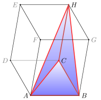
(a) The vertexes $A,B,C,H$ of $T_{1}$ as the corner points of the tetrahedron $C_{T_{1}}$.

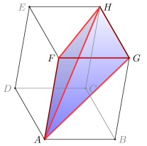
(b) The vertexes $A,F,G,H$ of $T_{2}$ as the corner points of the tetrahedron $C_{T_{2}}$.

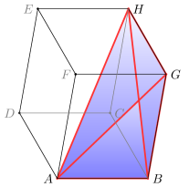
(c) The vertexes $A,B,G,H$ of $T_{3}$ as the corner points of the tetrahedron $C_{T_{3}}$.

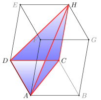
(d) The vertexes $A,D,C,H$ of $T_{4}$ as the corner points of the tetrahedron $C_{T_{4}}$.

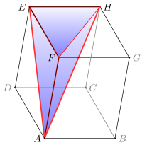
(e) The vertexes $A,F,E,H$ of $T_{5}$ as the corner points of the tetrahedron $C_{T_{5}}$.

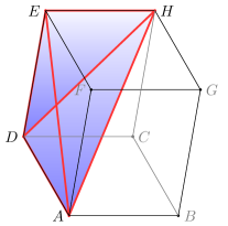
(f) The vertexes $A,D,E,H$ of $T_{6}$ as the corner points of the tetrahedron $C_{T_{6}}$.

Figure 1. The Coxeter-Freudenthal-Kuhn triangulation of the unit cube for $d=3$.

In this article, however, it is advantageous for technical reasons to have a partition of the unit cube $[0,1)^{d}$. As the polyhedrons $C_{T}$, $T\in\mathscr{T}_{1}^{0}$, do intersect on their boundary, we now slightly modify the sets to obtain a $d!$-sized family of sets $D_{T}$, indexed by $T\in\mathscr{T}_{1}^{0}$, with $D_{T}\subseteq C_{T}$ and

$$[0,1)^{d}\,=\,\dot{\bigcup_{T\in{\mathscr{T}}_{1}^{0}}}D_{T}.$$ (2.4)

The symbol $<_{\sigma,i}$ for $i\in\{2,\dots,d\}$ and $\sigma\in\mathscr{S}_{d}$ denotes the relation on $\mathbb{R}$ which coincides with ‘$<$’ in case $\sigma(i-1)<\sigma(i)$ and with ‘$\leq$’ in case $\sigma(i-1)>\sigma(i)$. Now we define

$$D_{T}\,:=\,\Big{\{}\,x\in\mathbb{R}^{d}\,\Big{|}\,0\leq x_{\sigma_{T}(d)}<_{\sigma_{T},d}x_{\sigma_{T}(d-1)}<_{\sigma_{T},d-1}\dots<_{\sigma_{T},2}x_{\sigma_{T}(1)}<1\,\Big{\}}.$$

Obviously, the topological closure $\overline{D_{T}}$ coincides with the convex hull $C_{T}$ of $\{T(i)|i=0,\dots,d\}$. Before we give a quick argumentation why 2.4 is satisfied with this definition, we remark that for reasons of symmetry the volume $|D_{T}|$ equals $1/(d!)$ under 2.4. Let now $x\in[0,1)^{d}$. To find the unique element $T\in\mathscr{T}_{1}^{0}$ such that $x\in D_{T}$ one simply takes the lexicographically ordered sequence, say $P_{1}>\dots>P_{d}$, of the tuples $\{(x_{i},i)|i=1,\dots,d\}$. Then one defines $\sigma(1)$ to be the second component of $P_{1}$, $\sigma(2)$ to be the second component of $P_{2}$, and so forth. It holds $x\in D_{T}$ if and only if $\sigma_{T}=\sigma$.

With the help of the sets $D_{T}$ we now construct certain piecewise linear, continuous functions on $\mathbb{R}^{d}$, which turn out useful in the context of Mosco convergence. For the moment $T\in\mathscr{T}_{1}^{0}$ is fixed. Let $i\in\{0,\dots,d\}$. The hyperplane in $\mathbb{R}^{d+1}$ which interpolates the sample $(T(j),\mathbb{1}_{\{i\}}(j))$, $j=0,\dots,d$, can be represented as the graph of the function

$$H_{T}^{i}:\,\mathbb{R}^{d}\,\ni\,x\,\longmapsto\,\begin{cases}\,1-x_{\sigma_{T}(1)}&\textnormal{if }i=0,\\ \,x_{\sigma_{T}(i)}-x_{\sigma_{T}(i+1)}&\textnormal{if }i\in\{1,\dots,d-1\}\textnormal{ and}\\ \,x_{\sigma_{T}(d)}&\textnormal{if }i=d.\end{cases}$$

Indeed, given $j\in\{0,\dots,d\}$ and $k\in\{1,\dots,d\}$, the $\sigma_{T}(k)$-th component of $T(j)$ equals $1$ if $j\geq k$, while the $\sigma_{T}(k)$-th component of $T(j)$ equals $0$ if $j<k$, due to 2.2. Hence, we verify

$$H_{T}^{i}(T(j))\,=\,\begin{cases}\,1-\mathbb{1}_{\{1,\dots,d\}}(j)\,&=\,\mathbb{1}_{\{i\}}(j)\quad\textnormal{if }i=0,\\ \,\mathbb{1}_{\{i,\dots,d\}}(j)-\mathbb{1}_{\{i+1,\dots,d\}}(j)&=\,\mathbb{1}_{\{i\}}(j)\quad\textnormal{if }i\in\{1,\dots,d-1\},\\ \,\mathbb{1}_{\{d\}}(j)&=\,\mathbb{1}_{\{i\}}(j)\quad\textnormal{if }i=d.\end{cases}$$

In particular, it holds

$$\sum_{i=0}^{d}H_{T}^{i}\,=\,\mathbb{1}_{\mathbb{R}^{d}}.$$ (2.5)

For $i\in\{0,\dots,d\}$ the gradient of $H_{T}^{i}$ is the constant vector

$$\sum_{k=1}^{d}\partial_{k}H^{i}_{T}\,\mathbb{e}_{k}\,=\,\mathbb{1}_{\{1,\dots,d\}}(i)\,\mathbb{e}_{\sigma_{T}(i)}-\mathbb{1}_{\{0,\dots,d-1\}}(i)\,\mathbb{e}_{\sigma_{T}(i+1)}.$$ (2.6)

Using 2.6 to calculate the euclidean scalar product of the gradients of $H_{T}^{i}$ and $H_{T}^{j}$ for $i,j\in\{0,\dots,d\}$ at a point $x\in\mathbb{R}^{d}$ we obtain

$$\sum_{k=1}^{d}\partial_{k}H^{i}_{T}(x)\,\partial_{k}H^{j}_{T}(x)\,=\,\begin{cases}\,\phantom{-}2&\textnormal{if }i=j\in\{1,\dots,d-1\},\\ \,\phantom{-}1&\textnormal{if }i=j\in\{0,d\},\\ \,-1&\textnormal{if }|i-j|=1\textnormal{ and}\\ \,\phantom{-}0&\textnormal{else.}\end{cases}$$ (2.7)

If we compose the function $\mathbb{1}_{D_{T}}\cdot H_{T}^{i}$ with the shift $\mathbb{R}^{d}\ni x\mapsto x+T(i)$ and sum up over all $T\in\mathscr{T}_{0}^{1}$ and $i=0,\dots,d$ we arrive at the definition of the the primal tent function

$$\chi_{1}^{0}:\mathbb{R}^{d}\ni x\,\mapsto\,\sum_{T\in\mathscr{T}_{1}^{0}}\sum_{i=0}^{d}\mathbb{1}_{D_{T}}(x+T(i))\,H_{T}^{i}(x+T(i)).$$

This piecewise definition glues together $(d+1)\,|\mathscr{T}_{1}^{0}|=(d+1)!$ many components, all of which are cut-off linear functions. For $T\in\mathscr{T}_{1}^{0}$ and $i=0,\dots,d$ the indicator function $\mathbb{1}_{D_{T}}(\,\cdot\,+T(i))$ $=\mathbb{1}_{D_{T}-T(i)}(\cdot)$ - up to a set of Lebesgue measure zero - weights the convex hull of the points

$$P_{0}:=T(0)-T(i),\,P_{1}:=T(1)-T(i),\,\dots,\,P_{d}:=T(d)-T(i).$$

$P_{0},\dots,P_{d}$ are the vertexes of a path of length $(d+1)$, which only travels in directions parallel to $\mathbb{e}_{1},\mathbb{e}_{2}\dots,$ or $\mathbb{e}_{d}$, uses each direction once, and visits the origin as its $i$-th vertex. The function $H_{T}^{i}(\,\cdot\,+T(i))$ is the linear interpolation of the sample ${(P_{j},\delta_{\{i\}}(j))}$, $j=0,\dots,d$, being $1$ in the origin and $0$ at all other nodes $P_{j}$, $j\neq i$. Figure 2(b) shows the graph of the primal tent function for the case $d=2$. Its support, highlighted in Figure 2(a), comprises six triangular domains.

These are

$$\overline{D}_{T_{1}},\qquad\qquad \phantom{-\mathbb{e}_{1}-\mathbb{e}_{2}+}\overline{D}_{T_{2}},$$

$$-\mathbb{e}_{1}+\overline{D}_{T_{1}},\qquad\qquad \phantom{-\mathbb{e}_{2}}-\mathbb{e}_{2}+\overline{D}_{T_{2}},$$

$$-\mathbb{e}_{1}-\mathbb{e}_{2}+\overline{D}_{T_{1}},\qquad\qquad -\mathbb{e}_{1}-\mathbb{e}_{2}+\overline{D}_{T_{2}},$$

where $T_{1},T_{2}$ are the two elements of $\mathscr{T}_{1}^{0}$ in the two-dimensional case, defined via 2.2 with $\sigma_{T_{1}}=(1,2)$ and $\sigma_{T_{2}}=(2,1)$.

(a) The six triangular domains comprising the support of $\chi_{1}^{0}$.

(b) The graph of $\chi_{1}^{0}$ in the $(2+1)$-dimensional space.

Figure 2. The primal tent function $\chi_{1}^{0}$ for $d=2$ with its hexagonal support.

The fact that $\chi_{1}^{0}$ is indeed an element of $\mathscr{C}$, i.e. a primal function, becomes evident in the proceeding part. We define the tent function with scaling parameter $r\in(0,\infty)$ and node $\alpha\in r\,\mathbb{Z}^{d}$ as $\chi_{r}^{\alpha}(x):=\chi_{1}^{0}((x-\alpha)/r)$, $x\in\mathbb{R}^{d}$. For $x\in\mathbb{R}^{d}$ it holds

$$\sum_{\alpha\in r\mathbb{Z}^{d}}\chi_{r}^{\alpha}(x)\,=\,\sum_{\beta\in\mathbb{Z}^{d}}\,\sum_{T\in\mathscr{T}_{1}^{0}}\,\sum_{i=0}^{d}\,\mathbb{1}_{D_{T}}\big{(}\,\frac{x}{r}+T(i)-\beta\,\big{)}\,H_{T}^{i}\big{(}\,\frac{x}{r}+T(i)-\beta\,\big{)}.$$ (2.8)

Since $D_{T}\subseteq[0,1)^{d}$, a summand of the right hand side can only yield a non-zero value if

$$\beta\,=\,\big{[}\,\frac{x}{r}+T(i)\,\big{]}\,=\,\big{[}\,\frac{x}{r}\,\big{]}+T(i).$$

Hence, with 2.5 and 2.4 we continue the calculation for the value of 2.8 by

$$\sum_{\alpha\in r\mathbb{Z}^{d}}\chi_{r}^{\alpha}(x)\, =\,\sum_{T\in\mathscr{T}_{1}^{0}}\,\sum_{i=0}^{d}\,\mathbb{1}_{D_{T}}\big{(}\,\frac{x}{r}-\big{[}\,\frac{x}{r}\,\big{]}\,\big{)}\,H_{T}^{i}\big{(}\,\frac{x}{r}-\big{[}\,\frac{x}{r}\,\big{]}\,\big{)}$$

$$=\,\sum_{T\in\mathscr{T}_{1}^{0}}\,\mathbb{1}_{D_{T}}\big{(}\,\frac{x}{r}-\big{[}\,\frac{x}{r}\,\big{]}\,\big{)}\,=\,1$$ (2.9)

for $x\in\mathbb{R}^{d}$. So, the family $\chi_{r}^{\alpha}$, $\alpha\in r\,\mathbb{Z}^{d}$ form a partition of unity for any $r\in(0,\infty)$. We sum up the properties which make it valuable for the proceeding discussion in 2.1. Before we state the theorem we introduce some further terminology. The rescaled family $r\,D_{T}$, $T\in\mathscr{T}_{1}^{0}$, partition the semi-open cube $[0,r)^{d}$ with side length $r$ for fixed $r\in(0,\infty)$. Hence the family $\alpha+r\,D_{T}$, over $\alpha\in r\,\mathbb{Z}^{d}$, $T\in\mathscr{T}_{1}^{0}$, form a partition of $\mathbb{R}^{d}$. For $r\in(0,\infty)$ we set

$$\mathscr{T}_{r}\,:=\,\bigcup_{\alpha\in r\mathbb{Z}^{d}}\alpha+r\,\mathscr{T}^{0}_{1}$$

and if $T=\alpha+r\,T^{\prime}\in\mathscr{T}_{1}^{0}$ with $T^{\prime}\in\mathscr{T}_{1}^{0}$, $\alpha\in r\,\mathbb{Z}^{d}$, then

$$D_{T}\,:=\,\alpha+r\,D_{T^{\prime}},\qquad\sigma_{T}\,:=\,\sigma_{T^{\prime}}.$$

Theorem 2.1.

Let $r\in(0,\infty)$. The space $\mathbb{R}^{d}$ admits a partition $\{D_{T}|T\in\mathscr{T}_{r}\}$ and a partition of unity ${(\chi_{r}^{\alpha})}_{\alpha\in r\mathbb{Z}^{d}}$ with the following properties.

1. $\int_{\mathbb{R}^{d}}\chi_{r}^{\alpha}\mathop{}\!\mathrm{d}x=r^{d}$ for $\alpha\in r\mathbb{Z}^{d}$.

2. For $\alpha\in r\mathbb{Z}^{d}$ the function $\chi_{r}^{\alpha}$ is continuous on $\mathbb{R}^{d}$ with values in $[0,1]$ and support on $\alpha+[-r,r]^{d}$.

3. Let $w\in\mathbb{R}^{(r\mathbb{Z}^{d})}$. The $i$-th weak partial derivative of the weighted sum $\sum_{\alpha}w_{\alpha}\,\chi_{r}^{\alpha}$ reads

   $$\sum_{\alpha\in r\mathbb{Z}^{d}}w_{\alpha}\partial_{i}\chi^{\alpha}_{r}\,=\,\frac{1}{r}\sum_{\alpha\in r\mathbb{Z}^{d}}\sum_{\begin{subarray}{c}T\in\mathscr{T}_{r}:\\ T(\sigma^{-1}_{T}(i)-1)=\alpha\end{subarray}}(w_{\alpha+r\mathbb{e}_{i}}-w_{\alpha})\,\mathbb{1}_{D_{T}}$$

   for $i=1,\dots,d$. The equality in the line above holds in $a.e.$-sense w.r.t. the Lebesgue measure on $\mathbb{R}^{d}$. Thus the function on the right hand side is a version of the weak partial derivative of the left hand side. The squared norm of the weak gradient calculates as

   $$\sum_{i=1}^{d}\Big{(}\sum_{\alpha\in r\mathbb{Z}^{d}}w_{\alpha}\,\partial_{i}\chi^{\alpha}_{r}\Big{)}^{2}\,=\,\frac{1}{r^{2}}\sum_{T\in\mathscr{T}_{r}}\mathbb{1}_{D_{T}}\sum_{i=1}^{d}\big{(}\,w_{T(i)}-w_{T(i-1)}\,\big{)}^{2}.$$

   Again, the equation holds in $a.e.$-sense and the function on the right hand side is a version of the left hand side.

Proof.

To proof (i) we use the shift invariance of the Lebesgue measure, the transformation formula of the integral and 2.5 to calculate

$$\int\limits_{\mathbb{R}^{d}}\chi_{r}^{\alpha}\mathop{}\!\mathrm{d}x\, =\,\sum_{T\in\mathscr{T}_{1}^{0}}\sum_{i=0}^{d}\int\limits_{\mathbb{R}^{d}}H_{T}^{i}\big{(}\frac{x}{r^{d}}\big{)}\mathop{}\!\mathrm{d}x$$

$$=\,r^{d}\,\sum_{T\in\mathscr{T}_{1}^{0}}\sum_{i=0}^{d}\int\limits_{\mathbb{R}^{d}}H_{T}^{i}(x)\mathop{}\!\mathrm{d}x\,=\,\sum_{T\in\mathscr{T}_{1}^{0}}r^{d}\int\limits_{\mathbb{R}^{d}}\mathbb{1}_{D_{T}}\mathop{}\!\mathrm{d}x\,=\,r^{d}.$$

for $\alpha\in r\,\mathbb{Z}^{d}$.

In Item (ii), only the continuity of $\chi_{r}^{\alpha}$ needs proof. We may restrict to the case $r=1$ and $\alpha=0\in\mathbb{Z}^{d}$. Since $\chi_{1}^{0}$ is a piecewise linear function, it is required to show $H^{i}_{T}(x-T(i))=H^{j}_{T^{\prime}}(x-T^{\prime}(j))$ for $T,T^{\prime}\in\mathscr{T}_{1}$ with $T(i)=T^{\prime}(j)=0$ and $x\in\overline{D_{T}}\cap\overline{D_{T^{\prime}}}$. This intersection coincides with the convex hull of $T\cap T^{\prime}$. If $T\cap T^{\prime}=\{0,P_{1},\dots,P_{m}\}$ is a set in $\mathbb{Z}^{d}$ of size $m+1$, then both $H^{i}_{T}(x-T(i))$ and $H^{j}_{T^{\prime}}(x-T^{\prime}(j))$ coincide with the evaluation at $x$ of the linear interpolation on the of the $m+1$ sized sample $(0,1)$, $(P_{i},0)$, $i=1,\dots m$ on the linear span of $T\cap T^{\prime}$, which is a $m+1$ dimensional subspace of $\mathbb{R}^{d}$.

To show (iii) we fix a point $x\in\mathbb{R}^{d}$ and choose the unique element $T\in\mathscr{T}_{r}$, say $T=\gamma+rT^{\prime}$ for some $T^{\prime}\in\mathscr{T}_{1}^{0}$, such that $x\in D_{T}=\gamma+rD_{T^{\prime}}$. We assume that $x$ is contained in the interior of $D_{T}$. This poses no restriction since the statements we want to show refer to an ‘a.e.’ way of reading and the boudary of $D_{T}$ has Lebesgue measure zero. Let $\alpha\in r\,\mathbb{Z}^{d}$. A necessary condition the support of the function $\chi_{r}^{\alpha}$ to contain $x$ is

$$x\in\alpha-r\,\tilde{T}(j)+r\,D_{\tilde{T}}\qquad\textnormal{for some }\tilde{T}\in\mathscr{T}_{1}^{0}\textnormal{ and }j=0,\dots,d.$$

Since $\mathscr{T}_{r}$ is a partition of $\mathbb{R}^{d}$, this condition is equivalent to

$$\tilde{T}=T^{\prime}\qquad\textnormal{with }\gamma=\alpha-r\tilde{T}(j)\qquad\textnormal{for some }j=0,\dots,d,$$

which is in turn equivalent to $\tilde{T}=T^{\prime}$ with $\alpha=\gamma+rT^{\prime}(j)$ $(=T(j))$ for some $j=0,\dots,d$. Using these equivalences, we conclude that for each point $y$ from the interior of $D_{T}$ it holds

$$\chi^{T(j)}_{r}(y)\,=\,H^{j}_{T^{\prime}}\big{(}\,\frac{y-T(j)}{r}+T^{\prime}(j)\,\big{)}\,=\,H^{j}_{T^{\prime}}\big{(}\,\frac{y-\gamma}{r}\,\big{)}.$$

Therefore, for $i\in\{1,\dots,d\}$, we compute, using 2.6 in the third equality,

$$\sum_{\alpha\in r\mathbb{Z}^{d}}w_{\alpha}\,\partial_{i}\chi_{r}^{\alpha}(x)\,=\,\sum_{\alpha\in T}w_{\alpha}\,\partial_{i}\chi_{r}^{\alpha}(x)\,=\,\sum_{j=0}^{d}w_{T(j)}\,\frac{1}{r}\,\partial_{i}H^{j}_{T^{\prime}}\big{(}\,\frac{x-\gamma}{r}\,\big{)}\\ =\,\frac{1}{r}\sum_{j=0}^{d}w_{T(j)}\,{\Big{(}\,\mathbb{1}_{\{1,\dots,d\}}(j)\,\mathbb{e}_{\sigma_{T}(j)}-\mathbb{1}_{\{0,\dots,d-1\}}(j)\,\mathbb{e}_{\sigma_{T}(j+1)}\,\Big{)}}^{\textnormal{T}}\mathbb{e}_{i}\\ =\,\frac{1}{r}\sum_{j=1}^{d}w_{T(j)}\,\mathbb{1}_{\{i\}}(\sigma_{T}(j))-\sum_{j=0}^{d-1}w_{T(j)}\,\mathbb{1}_{\{i\}}(\sigma_{T}(j+1))\\ =\,\frac{1}{r}\,\big{(}\,w_{T(\sigma_{T}^{-1}(i))}-w_{T(\sigma_{T}^{-1}(i)-1)}\,\big{)}\\ =\,\frac{1}{r}\,\big{(}\,w_{T(\sigma_{T}^{-1}(i)-1)+r\mathbb{e}_{i}}-w_{T(\sigma_{T}^{-1}(i)-1)}\,\big{)}.$$ (2.10)

The last equality holds due to 2.1. Consequently,

$$\sum_{\alpha\in r\mathbb{Z}^{d}}w_{\alpha}\,\partial_{i}\chi_{r}^{\alpha}(x)\, =\,\frac{1}{r}\,\sum_{S\in\mathscr{T}_{r}}\big{(}\,w_{T(\sigma_{S}^{-1}(i)-1)+r\mathbb{e}_{i}}-w_{T(\sigma_{S}^{-1}(i)-1)}\,\big{)}\,\mathbb{1}_{D_{S}}(x)$$

$$=\,\frac{1}{r}\,\sum_{\alpha\in r\mathbb{Z}^{d}}\,\sum_{\begin{subarray}{c}S\in\mathscr{T}_{r}:\\ T(\sigma_{S}^{-1}(i)-1)=\alpha\end{subarray}}\big{(}\,w_{T(\sigma_{S}^{-1}(i)-1)+r\mathbb{e}_{i}}-w_{T(\sigma_{S}^{-1}(i)-1)}\,\big{)}\,\mathbb{1}_{D_{S}}(x)$$

as desired. To calculate the squared norm of the weak gradient, we sum up the squared values of 2.10 over the index $i=1,\dots d$ and obtain

$$\sum_{i=1}^{d}\Big{(}\sum_{\alpha\in r\mathbb{Z}^{d}}w_{\alpha}\,\partial_{i}\chi^{\alpha}_{r}\Big{)}^{2}(x)\,=\,\frac{1}{r^{2}}\,\sum_{i=1}^{d}{\big{(}\,w_{T(\sigma_{T}^{-1}(i)-1)+r\mathbb{e}_{i}}-w_{T(\sigma_{T}^{-1}(i)-1)}\,\big{)}}^{2}\\ =\,\frac{1}{r^{2}}\,\sum_{\begin{subarray}{c}j\in\{1,\dots,d\}:\\ \sigma_{T}(j)=i\end{subarray}}{\big{(}\,w_{T(j-1)+r\mathbb{e}_{\sigma_{T}(j)}}-w_{T(j-1)}\,\big{)}}^{2}\,=\,\frac{1}{r^{2}}\,\sum_{j=1}^{d}\big{(}\,w_{T(j)}-w_{T(j-1)}\,\big{)}^{2}.\\$$

The last equality holds due to 2.1 and concludes the proof, because $\sum_{S\in\mathscr{T}_{r}}\mathbb{1}_{D_{S}}(x)=1$. ∎

2.2. $L^{2}$ and energy estimates

In this section we investigate the approximative quality of such weighted sums as have been considered in 2.1 (iii) regarding certain symmetric bilinear forms of $L^{2}$ and energy type. Let $\varrho:\mathbb{R}^{d}\to[0,\infty)$ be a probability density w.r.t. the Lebesgue measure on $\mathbb{R}^{d}$. The energy

$$E^{\varrho}(f,g)\,:=\,\int\limits_{\mathbb{R}^{d}}\Gamma(f,g)\,\varrho\mathop{}\!\mathrm{d}x\qquad\textnormal{with}\qquad\Gamma(f,g)\,:=\,\sum_{i=1}^{d}\partial_{i}f\,\partial_{i}g$$

shall be defined for $f,g\in\mathscr{D}$. We denote by

$$\mathscr{D}:=\Big{\{}\,f\in C_{\textnormal{b}}(\mathbb{R}^{d})\,\Big{|}\,\partial_{i}f\textnormal{ exists in weak sense and }\partial_{i}f\in L^{\infty}(\mathbb{R}^{d},\mathop{}\!\mathrm{d}x)\textnormal{ for }i=1,\dots,d\,\Big{\}}.$$

that linear subspace of the bounded, continuous functions $C_{\textnormal{b}}(\mathbb{R}^{d})$ whose elements are representatives for elements of the Sobolev space $H^{1,\infty}(\mathbb{R}^{d})$. The resulting Lemma is the key ingredient to the principle theorem of this paper, 3.11 of the next section. The approximative quality translates into conditions on the density $\varrho$ in terms of the $\varphi,\eta$-residual $R_{r}^{\varphi,\eta}(\varrho)$ and the $\varphi,\eta$-perturbation $I_{r}^{\varphi,\eta}(\varrho)$. These quantities are defined depending on the primal functions $\varphi,\eta:\mathbb{R}^{d}\to[0,1]$ and the parameter $r\in(0,\infty)$, as mappings from the set of non-negative, integrable functions into itself.

$$R_{r}^{\varphi,\eta}(g) \,:=\,\sum_{\alpha\in r\mathbb{Z}^{d}}r^{-d}\int\limits_{\mathbb{R}^{d}}|g(\,\cdot\,)-g(x)|\,\eta_{r}^{\alpha}(x)\mathop{}\!\mathrm{d}x\,\varphi_{r}^{\alpha}(\,\cdot\,)$$ (2.11)

$$\textnormal{and}\quad I_{r}^{\varphi,\eta}(g) \,:=\,\sum_{\alpha\in r\mathbb{Z}^{d}}r^{-d}\int\limits_{\mathbb{R}^{d}}\eta_{r}^{\alpha}(x)\,g(x)\mathop{}\!\mathrm{d}x\,\varphi_{r}^{\alpha}(\,\cdot\,)$$ (2.12)

for a non-negative, measurable function $g\in\mathcal{M}_{+}(\mathbb{R}^{d})$ with $\int_{\mathbb{R}^{d}}g\mathop{}\!\mathrm{d}x<\infty$. Since

$$\int\limits_{\mathbb{R}^{d}}\eta_{r}^{\alpha}(x)\mathop{}\!\mathrm{d}x\,=\,r^{d}\qquad\textnormal{and}\qquad\int\limits_{\mathbb{R}^{d}}\varphi_{r}^{\alpha}(x)\mathop{}\!\mathrm{d}x\,=\,r^{d},$$

it holds

$$\int\limits_{\mathbb{R}^{d}}I_{r}^{\varphi,\eta}(g)\,(x)\mathop{}\!\mathrm{d}x\,=\,\sum_{\alpha\in r\mathbb{Z}^{d}}\,\int\limits_{\mathbb{R}^{d}}g(x)\,\eta_{r}^{\alpha}(x)\mathop{}\!\mathrm{d}x\,=\,\int\limits_{\mathbb{R}^{d}}g\mathop{}\!\mathrm{d}x$$

as well as

$$\int\limits_{\mathbb{R}^{d}}R_{r}^{\varphi,\eta}(g)\,(x)\mathop{}\!\mathrm{d}x\,\leq\,\int\limits_{\mathbb{R}^{d}}\,\sum_{\alpha\in r\mathbb{Z}^{d}}r^{-d}\int\limits_{\mathbb{R}^{d}}g(y)+g(x)\,\eta_{r}^{\alpha}(x)\mathop{}\!\mathrm{d}x\,\varphi_{r}^{\alpha}(y)\mathop{}\!\mathrm{d}y\\ =\,\sum_{\alpha\in r\mathbb{Z}^{d}}\,\int\limits_{\mathbb{R}^{d}}g(y)\,\varphi_{r}^{\alpha}(y)\mathop{}\!\mathrm{d}y+\sum_{\alpha\in r\mathbb{Z}^{d}}\,\int\limits_{\mathbb{R}^{d}}g(x)\,\eta_{r}^{\alpha}(x)\mathop{}\!\mathrm{d}x\,=\,2\int\limits_{\mathbb{R}^{d}}g(x)\mathop{}\!\mathrm{d}x$$

for $g\in\mathcal{M}_{+}(\mathbb{R}^{d})$. Let $m:=\varrho\,\mathop{}\!\mathrm{d}x$. The space of bounded measurable functions $\mathcal{M}_{\textnormal{b}}(\mathbb{R}^{d})$ is dense in $L^{2}(\mathbb{R}^{d},m)$. We use the convention $1/0=\infty$ and $\infty\cdot 0=0$. For a measurable function $\kappa:\mathbb{R}^{d}\to[0,1]$ we set

$$\delta^{\kappa}_{r}(m) \,:=\,\sup_{\varphi,\eta\in\mathscr{C}}\,\sup_{f\in\mathcal{M}_{\textnormal{b}}(\mathbb{R}^{d})}\,\frac{|\int_{\mathbb{R}^{d}}f(x)\,R_{r}^{\varphi,\eta}(\kappa\,\varrho)\,(x)\mathop{}\!\mathrm{d}x\,|}{\|f\|_{L^{2}(m)}}\,\in\mathbb{R}_{0}^{+}\cup\{\infty\}$$ (2.13)

$$\textnormal{and}\quad C^{\kappa}_{r}(m) \,:=\,\sup_{\varphi,\eta\in\mathscr{C}}\,\sup_{f\in\mathcal{M}_{\textnormal{b}}(\mathbb{R}^{d})}\,\frac{|\int_{\mathbb{R}^{d}}f(x)\,I_{r}^{\varphi,\eta}(\kappa\,\varrho)\,(x)\mathop{}\!\mathrm{d}x\,|}{\|f\|_{L^{1}(m)}}\in\mathbb{R}_{0}^{+}\cup\{\infty\}.$$ (2.14)

A finite value for $C^{\kappa}_{r}(m)$ allows to extend the linear functional $f\mapsto$ $\int_{\mathbb{R}^{d}}\,f(x)\,I_{r}^{\varphi,\eta}(\kappa\,\varrho)(x)\mathop{}\!\mathrm{d}x$ to an element from the dual of $L^{1}(\mathbb{R}^{d},m)$ with norm smaller equal $C^{\kappa}_{r}(m)$ via the BLT theorem. In the same way, a finite value for $\delta^{\kappa}_{r}(m)$ allows to extend the linear functional $f\mapsto$ $\int_{\mathbb{R}^{d}}\,f(x)\,R_{r}^{\varphi,\eta}(\kappa\,\varrho)(x)\mathop{}\!\mathrm{d}x$ to an element from the dual of $L^{2}(\mathbb{R}^{d},m)$ with norm smaller equal $\delta^{\kappa}_{r}(m)$. We hint at a consequence of the Riesz isomorphism.

Remark 2.2.

Let $R\in\mathcal{M}_{+}(\mathbb{R}^{d})$ with $\int_{\mathbb{R}^{d}}R\mathop{}\!\mathrm{d}x<\infty$.

$$\sup_{f\in\mathcal{M}_{\textnormal{b}}(\mathbb{R}^{d})}\,\frac{|\int_{\mathbb{R}^{d}}f(x)\,R(x)\mathop{}\!\mathrm{d}x\,|}{\|f\|_{L^{2}(m)}}\,=:\,D<\infty$$

if and only if there exists $\hat{R}\in L^{2}(\mathbb{R}^{d},m)$ with $\|\hat{R}\|_{L^{2}(m)}=D$ and

$$\int\limits_{\mathbb{R}^{d}}f(x)\,R(x)\mathop{}\!\mathrm{d}x\,=\,\int\limits_{\mathbb{R}^{d}}f(x)\,\hat{R}(x)\,\varrho(x)\,\mathop{}\!\mathrm{d}x.$$

for $f\in\mathcal{M}_{\textnormal{b}}(\mathbb{R}^{d})$. The latter is equivalent to $R/\varrho\in L^{2}(m)$ with

$$D\,:=\,\Big{(}\int\limits_{\mathbb{R}^{d}}|R(x)|^{2}\,\frac{1}{\varrho(x)}\mathop{}\!\mathrm{d}x\Big{)}^{\frac{1}{2}}.$$

To make the analysis useful for the purpose of the next section we consider direct integrals of such energies. For a Polish space $S$ we denote the Borel $\sigma$-algebra by $\mathcal{B}(S)$ and the bounded, measurable functions from $S$ to $\mathbb{R}$ by $\mathcal{M}_{\textnormal{b}}(S)$. Let $(S,\mathcal{B}(S),\nu)$ be a probability space over a Polish space $S$. We assume

$$\mathop{}\!\mathrm{d}m_{s}(x)\,:=\,\varrho(s,x)\mathop{}\!\mathrm{d}x$$

is a probability measure on $\mathbb{R}^{d}$ with density $\varrho(s,\,\cdot\,)$ for $s\in S$. Moreover, let $S\ni s\mapsto m_{s}(A)\in[0,1]$ be measurable for $A\in\mathcal{B}(\mathbb{R}^{d})$. The direct integral then reads

$$\big{(}\textstyle\int^{\oplus}\displaystyle E^{\varrho(s,\cdot)}\mathop{}\!\mathrm{d}\nu\big{)}(u,v)\,:=\,\int\limits_{S}E^{\varrho(s,\cdot)}\big{(}u(s,\cdot),v(s,\cdot)\big{)}\mathop{}\!\mathrm{d}\nu(s)$$

for $u,v$ from its domain

$$\mathcal{D}\big{(}\textstyle{\int^{\oplus}}E^{\varrho(s,\cdot)}\mathop{}\!\mathrm{d}\nu\big{)}\,:=\Big{\{}\,u\in\mathcal{M}_{\textnormal{b}}(S\times\mathbb{R}^{d})\,\Big{|}\, u(s,\cdot)\in\mathscr{D}\textnormal{ for }s\in S\textnormal{ and}$$

$$S\ni s\,\mapsto\,E^{\varrho(s,\cdot)}(u(s,\cdot),u(s,\cdot))$$

$$\textnormal{ is measurable and integrable w.r.t.\leavevmode\nobreak\ }\nu\,\Big{\}}.$$

For given $r\in(0,\infty)$ we recall the family $\chi_{r}^{\alpha}$, $\alpha\in r\,\mathbb{Z}^{d}$, from Section 2.1 and define a linear subspace of $\mathcal{D}\big{(}\textstyle{\int^{\oplus}}E^{\varrho(s,\cdot)}\mathop{}\!\mathrm{d}\nu\big{)}$ by

$$\mathscr{L}_{r}\,:=\,\Big{\{}\lambda:S\times\mathbb{R}^{d}\to\mathbb{R}\,\Big{|}\, \textnormal{there exists }M\in(0,\infty)\textnormal{ such that}$$

$$\begin{aligned} \lambda(s,x)=\sum_{\alpha\in r\mathbb{Z}^{d}}\lambda^{\alpha}(s)\,\chi_{r}^{\alpha}(x),\,s\in S,x\in\mathbb{R}^{d},\,\textnormal{with}&\\ \textnormal{measurable }\lambda^{\alpha}:S\to[-M,M]\textnormal{ for }\alpha\in r\,\mathbb{Z}^{d}&\,\Big{\}}.\end{aligned}$$

Since the support of $\chi_{r}^{\alpha}$ is contained in the cube $\alpha+[-r,r]^{d}$ for every $\alpha\in r\,Z^{d}$ and $r\in(0,\infty)$, the number of indexes $\alpha$ for which, at a point given point $x\in\mathbb{R}^{d}$, the function $\chi_{r}^{\alpha}$ does not vanish at $x$ is bounded by $2^{d}$. Therefore, $\mathscr{L}_{r}$ is a subspace of $\mathcal{M}_{\textnormal{b}}(S\times\mathbb{R}^{d})$ for every $r\in(0,\infty)$. The approximative qualities of the subspace $\mathscr{L}_{r}$ are in the focus of the next Lemma. For $g\in C_{\textnormal{c}}(\mathbb{R}^{d})$ and $\varepsilon\in(0,\infty)$, the continuous functions on $\mathbb{R}^{d}$ with compact support, we write

$$\omega_{\varepsilon}^{g}\,:=\,\sup_{\begin{subarray}{c}x,y\in\mathbb{R}^{d}\\ \textnormal{max}_{j}|x_{j}-y_{j}|\leq 4\varepsilon\end{subarray}}|g(x)-g(y)|\,.$$ (2.15)

Furthermore, if $g\in C^{1}_{\textnormal{c}}(\mathbb{R}^{d})$, the continuously differentiable functions on $\mathbb{R}^{d}$ with compact support, then

$$\omega_{\varepsilon}^{\nabla g}\,:=\,\max_{i=1,\dots,d}\,\omega_{\varepsilon}^{\partial_{i}g}\qquad\textnormal{and}\qquad D^{g}\,:=\max_{i=1,\dots,d}\|\partial_{i}g\|_{\infty}\,.$$

Lemma 2.3.

Let $f\in\mathcal{M}_{\textnormal{b}}(S)$, $g\in C^{1}_{\textnormal{c}}(\mathbb{R}^{d})$ and $\kappa:S\times\mathbb{R}^{d}\to[0,1]$ be measurable. For $u\in\mathcal{D}(\int^{\oplus}E^{\varrho(s,\cdot)}\mathop{}\!\mathrm{d}\nu)$ with $-1\leq u(\cdot)\leq 1$ and $r\in(0,\infty)$ there exists $\lambda\in\mathscr{L}_{r}$ such that each of the inequalities holds true.

1. $|\lambda^{\alpha}(\,\cdot\,)|\,\leq\,1$ where $\lambda^{\alpha}$ is the coefficient of $\lambda$ with index $\alpha\in r\,\mathbb{Z}^{d}$.

2. $\displaystyle\Big{|}\int\limits_{S\times\mathbb{R}^{d}}f(s)\,g(x)\,\big{(}u(s,x)-\lambda(s,x)\big{)}\,\kappa(s,x)\mathop{}\!\mathrm{d}m_{s}(x)\mathop{}\!\mathrm{d}\nu(s)\,\Big{|}$
   $\phantom{(ii)}\,\displaystyle\leq\,\|f\|_{L^{\infty}(\nu)}\,\big{(}\omega_{r}^{g}+\|g\|_{\infty}\,\|\delta^{\kappa(s,\cdot)}_{r}(m_{s})\|_{L^{2}(\nu)}\big{)}\,.$

3. $\displaystyle\Big{|}\int\limits_{S}f(s)\,E^{\kappa\varrho(s,\cdot)}\big{(}g,u(s,\cdot)-\lambda(s,\cdot)\big{)}\mathop{}\!\mathrm{d}\nu(s)\,\Big{|}$
   $\phantom{(iii)}\,\displaystyle\leq\,\sqrt{d}\,\|f\|_{L^{\infty}(\nu)}\,\big{(}\omega_{r}^{\nabla g}+D^{g}\,\|\delta^{\kappa(s,\cdot)}_{r}(m_{s})\|_{L^{2}(\nu)}\big{)}\,\Big{(}\int\limits_{S}E^{\varrho(s,\cdot)}\big{(}u(s,\cdot),u(s,\cdot)\big{)}\mathop{}\!\mathrm{d}\nu(s)\Big{)}^{\frac{1}{2}}\,.$

4. $\displaystyle\int\limits_{S}E^{\kappa\varrho(s,\cdot)}\big{(}\lambda(s,\cdot),\lambda(s,\cdot)\big{)}\mathop{}\!\mathrm{d}\nu(s)$ $\,\displaystyle\leq\,\|C^{\kappa(s,\cdot)}_{r}(m_{s})\|_{L^{\infty}(\nu)}\,\int\limits_{S}E^{\varrho(s,\cdot)}\big{(}u(s,\cdot),u(s,\cdot)\big{)}\mathop{}\!\mathrm{d}\nu(s).$

Proof.

Let $r\in(0,\infty)$ be fixed throughout this proof. We start with an abstract estimate, which will be used in two separate instances in the subsequent course of this proof. By $\rho:\mathbb{R}^{d}\to[0,\infty)$ we denote a generic non-negative, measurable function with $\int\rho\mathop{}\!\mathrm{d}x\leq 1$. Let $\varphi$, $\eta$ denote two generic elements from $\mathscr{C}$ and $h\in C_{\textnormal{c}}(\mathbb{R}^{d})$. Since the family ${(\varphi_{r}^{\alpha})}_{\alpha}$ sum up to one and $r^{-d}\eta_{r}^{\alpha}$ is a probability density for $\alpha\in r\,\mathbb{Z}^{d}$, we estimate

$$\Big{|}\,h(x)\,\rho(x)-\sum_{\alpha\in r\mathbb{Z}^{d}}\varphi^{\alpha}_{r}(x)\,r^{-d}\int\limits_{\mathbb{R}^{d}}\eta_{r}^{\alpha}(y)\,h(y)\,\rho(y)\mathop{}\!\mathrm{d}y\,\Big{|}\\ \begin{array}[]{lr}\displaystyle=\,\Big{|}\sum_{\alpha\in r\mathbb{Z}^{d}}\varphi^{\alpha}_{r}(x)\,r^{-d}\int\limits_{\mathbb{R}^{d}}(h(x)\,\rho(x)-h(y)\,\rho(y))\,\eta_{r}^{\alpha}(y)\mathop{}\!\mathrm{d}y\Big{|}&\\ \displaystyle\leq\,\sum_{\alpha\in r\mathbb{Z}^{d}}\varphi^{\alpha}_{r}(x)\,\Big{(}\omega_{r}^{h}\,\rho(x)+\|h\|_{\infty}\,r^{-d}\int\limits_{\mathbb{R}^{d}}|\rho(x)-\rho(y)|\,\eta_{r}^{\alpha}(y)\mathop{}\!\mathrm{d}y\Big{)}&\\ \displaystyle\leq\,\omega_{r}^{h}\,\rho(x)+\|h\|_{\infty}\,R^{\varphi,\eta}_{r}(\rho)(x)&\textup{\tagform@{2.16}}\end{array}$$

for each point $x\in\mathbb{R}^{d}$.

As in the claim of this lemma, we fix $u\in\mathcal{D}(\int^{\oplus}E^{\varrho(s,\cdot)}\mathop{}\!\mathrm{d}\nu)\cap\mathcal{M}(S\times\mathbb{R}^{d},[-1,1])$, $g\in C^{1}_{\textnormal{c}}(\mathbb{R}^{d})$ and $f\in\mathcal{M}_{\textnormal{b}}(S)$. The definition

$$\lambda(s,x)\,:=\,\sum_{\alpha\in r\mathbb{Z}^{d}}\frac{1}{r^{d}}\int\limits_{\mathbb{R}^{d}}u(s,y)\,\mathbb{1}_{(-r,0]^{d}}(\alpha-y)\mathop{}\!\mathrm{d}y\,\chi_{r}^{\alpha}(x)$$ (2.17)

for $x\in\mathbb{R}^{d}$ and $s\in S$ is in accordance with (i). We now dedicate ourselves to the verification of (ii) to (iv).

We start with Item (ii). The integrals, which needs to be computed, involves only integrands of bounded functions. By linearity, we obtain

$$\Big{|}\int\limits_{S\times\mathbb{R}^{d}}f(s)\,g(x)\,\big{(}u(s,x)-\lambda(s,x)\big{)}\,\kappa(s,x)\,\mathop{}\!\mathrm{d}m_{s}(x)\mathop{}\!\mathrm{d}\nu(s)\,\Big{|}\\ \begin{array}[]{lr}\displaystyle=\,\Big{|}\int\limits_{S\times\mathbb{R}^{d}}f(s)\,u(s,x)\,g(x)\,\kappa(s,x)\,\mathop{}\!\mathrm{d}m_{s}(x)\mathop{}\!\mathrm{d}\nu(s)&\\ \displaystyle\phantom{=}\,-\int\limits_{S}\int\limits_{\mathbb{R}^{d}}f(s)\,u(s,x)\sum_{\alpha\in r\mathbb{Z}^{d}}\Big{(}\mathbb{1}_{(-r,0]^{d}}(\alpha-x)\,r^{-d}\int\limits_{\mathbb{R}^{d}}g(y)\,\chi_{r}^{\alpha}(y)\mathop{}\!\mathrm{d}m_{s}(y)\Big{)}\mathop{}\!\mathrm{d}x\mathop{}\!\mathrm{d}\nu(s)\Big{|}.&\textup{\tagform@{2.18}}\end{array}$$

To get the subtracting term into the form as it is written in the line above, we plug in 2.17, use Fubini’s theorem and after changing the order of integration we also exchange the names of the variables $x$ and $y$. To go on, we put the subtraction inside the integral again and for each $s\in S$ and $x\in\mathbb{R}^{d}$ use Equation (2.16)with the choices $\kappa(s,\cdot)\,\varrho(s,\cdot)$ as $\rho$, $\mathbb{1}_{[0,1)^{d}}$ as $\varphi$, the tent function $\chi_{1}^{0}$ as $\eta$ and $h=g$, to estimate Equation (2.18)from above with

$$\int\limits_{S}\int\limits_{\mathbb{R}^{d}}|f(s)\,u(s,x)|\,\Big{(}\,\omega_{r}^{g}\,\kappa(s,x)\,\varrho(s,x)+\,\|g\|_{\infty}\,R^{\mathbb{1}_{[0,1)},\chi_{1}^{0}}_{r}((\kappa\,\varrho)(s,\cdot))\,(x)\,\Big{)}\mathop{}\!\mathrm{d}x\mathop{}\!\mathrm{d}\nu(s)\\ \begin{aligned} &\leq\,\omega_{r}^{g}\,\|f\|_{L^{\infty}(\nu)}\int\limits_{S}\int\limits_{\mathbb{R}^{d}}|u(s,x)|\mathop{}\!\mathrm{d}m_{s}(x)\mathop{}\!\mathrm{d}\nu(s)\\ &\phantom{\leq}\,+\|g\|_{\infty}\,\|f\|_{L^{\infty}(\nu)}\,\int\limits_{S}\delta_{r}^{\kappa(s,\cdot)}(m_{s})\,\Big{(}\int\limits_{\mathbb{R}^{d}}|u(s,x)|^{2}\mathop{}\!\mathrm{d}m_{s}(x)\Big{)}^{\frac{1}{2}}\mathop{}\!\mathrm{d}\nu(s).\end{aligned}$$

The claim of (ii) now follows with the Cauchy-Schwartz inequality.

We now turn to the proof of (iii). We fix $i\in\{1,\dots,d\}$. For $\alpha\in r\,\mathbb{Z}^{d}$ and $q\in(0,\infty)$ we set

$$\mathscr{T}_{q}^{\alpha,i}:=\Big{\{}T\in\mathscr{T}_{q}\,\Big{|}\,T(\sigma_{T}^{-1}(i)-1)=\alpha\Big{\}}$$

with the notation of Section 2.1. In view of 2.1 this condition means, that after hitting $\alpha$ the path of $T$ takes the direction of $\mathbb{e}_{i}$ until it reaches the next point on the lattice $\alpha+q\,\mathbb{e}_{i}$. We note, that by definition of $\mathscr{T}_{q}$ and 2.2 an element from $T\in\mathscr{T}_{q}$ is already uniquely defined if we are given its corresponding permutation $\sigma_{T}\in\mathscr{S}_{d}$ and one of its vertexes $T(j)\in q\,\mathbb{Z}^{d}$ for an arbitrary index $j\in\{0,\dots,d\}$. So, the size of $\mathscr{T}_{q}^{0,i}$ calculates as

$$|\mathscr{T}_{q}^{0,i}|\, =\,\sum_{j=0}^{d-1}\Big{|}\Big{\{}T\in\mathscr{T}_{q}\,\Big{|}\,T(j)=0\textnormal{ and }\,T(\sigma_{T}^{-1}(i)-1)=T(j)\Big{\}}\Big{|}$$

$$=\,\sum_{j=0}^{d-1}\Big{|}\Big{\{}T\in\mathscr{T}_{q}\,\Big{|}\,T(j)=0\textnormal{ and }\,\sigma_{T}(j+1)=i\Big{\}}\Big{|}$$

$$=(d-1)!\,d=d!.$$

Hence,

$$\tilde{\eta}:=\sum_{T\in\mathscr{T}_{1}^{0,i}}\mathbb{1}_{D_{T}}$$

defines an element from $\mathscr{C}$, because $|D_{T}|=1/(d!)$ for $T\in\mathscr{T}_{1}$ and moreover

$$\sum_{\alpha\in\mathbb{Z}^{d}}\tilde{\eta}_{1}^{\alpha}\,=\,\sum_{\alpha\in\mathbb{Z}^{d}}\sum_{T\in\mathscr{T}_{1}^{\alpha,i}}\mathbb{1}_{D_{T}}\,=\sum_{T\in\mathscr{T}_{1}}\mathbb{1}_{D_{T}}\,=\,1.$$

We define another element from $\mathscr{C}$,

$$\tilde{\varphi}:\mathbb{R}^{d}\ni y\mapsto\int_{0}^{1}\mathbb{1}_{[0,1)^{d}}(y-t\,\mathbb{e}_{i})\mathop{}\!\mathrm{d}t.$$

Let $s\in S$ and $i=\{1,\dots,d\}$. The main effort in the proof of the estimate of (iii) is done by a preliminary transformation of a relevant integral. To shorten the notation in the next lines we set

$$I_{T}\,:=\,\int\limits_{D_{T}}\partial_{i}g(x)\,\kappa(s,x)\,\varrho(s,x)\mathop{}\!\mathrm{d}x$$

for $T\in\mathscr{T}_{r}$. To obtain the equivalences as follows, we first use Fubini’s theorem, then apply 2.1 (iii) before we use the translation invariance of the Lebesgue measure and the fundamental theorem of calculus.

$$\int\limits_{\mathbb{R}^{d}}\partial_{x_{i}}\lambda(s,x)\,\partial_{i}g(x)\,\kappa(s,x)\mathop{}\!\mathrm{d}m_{s}(x)$$

$$=\sum_{\alpha\in r\mathbb{Z}^{d}}r^{-d}\int\limits_{\mathbb{R}^{d}}u(s,y)\,\mathbb{1}_{(-r,0]}(\alpha-y)\mathop{}\!\mathrm{d}y\int\limits_{\mathbb{R}^{d}}\partial_{i}\chi^{\alpha}_{r}(x)\,\partial_{i}g(x)\,(\kappa\,\varrho)(s,x)\mathop{}\!\mathrm{d}x$$

$$=\,\sum_{\alpha\in r\mathbb{Z}^{d}}\sum_{T\in\mathscr{T}_{r}^{\alpha,i}}r^{-d-1}\int\limits_{\mathbb{R}^{d}}u(s,y)\,\big{(}\mathbb{1}_{(-r,0]}(\alpha+r\,\mathbb{e}_{i}-y)-\mathbb{1}_{(-r,0]}(\alpha-y)\big{)}\mathop{}\!\mathrm{d}y\,I_{T}$$

$$=\,\sum_{\alpha\in r\mathbb{Z}^{d}}\sum_{T\in\mathscr{T}_{r}^{\alpha,i}}r^{-d-1}\int\limits_{\mathbb{R}^{d}}\big{(}u(s,y+r\,\mathbb{e}_{i})-u(s,y)\big{)}\,\mathbb{1}_{(-r,0]}(\alpha-y)\mathop{}\!\mathrm{d}y\,I_{T}$$

$$=\,\sum_{\alpha\in r\mathbb{Z}^{d}}\sum_{T\in\mathscr{T}_{r}^{\alpha,i}}r^{-d-1}\int\limits_{\mathbb{R}^{d}}\int_{0}^{r}\frac{\partial u(s,x+t\,\mathbb{e}_{i})}{\partial x_{i}}\mathop{}\!\mathrm{d}t\,\mathbb{1}_{(-r,0]}(\alpha-x)\mathop{}\!\mathrm{d}x\,I_{T}$$

$$=\,\sum_{\alpha\in r\mathbb{Z}^{d}}\sum_{T\in\mathscr{T}_{r}^{\alpha,i}}r^{-d-1}\int\limits_{\mathbb{R}^{d}}\partial_{i}^{x}u(s,x)\int_{0}^{r}\mathbb{1}_{(-r,0]}(\alpha-x+t\,\mathbb{e}_{i})\mathop{}\!\mathrm{d}t\mathop{}\!\mathrm{d}x\,I_{T}$$

$$=\,\int\limits_{\mathbb{R}^{d}}\partial_{i}^{x}u(s,x)\,\sum_{\alpha\in r\mathbb{Z}^{d}}\tilde{\varphi}_{r}^{\alpha}(x)\,r^{-d}\,\int\limits_{\mathbb{R}^{d}}\tilde{\eta}_{r}^{\alpha}(y)\,\partial_{i}g(y)\,(\kappa\,\varrho)(s,y)\mathop{}\!\mathrm{d}y\mathop{}\!\mathrm{d}x.$$ (2.19)

In the second to last step we change the order in which we integrate w.r.t. $\mathop{}\!\mathrm{d}t$ and $\mathop{}\!\mathrm{d}x_{i}$, then use the translation invariance of $\mathop{}\!\mathrm{d}x_{i}$ before we change back. If we subtract the integral calculated in Section 2.2 from the term $\int_{\mathbb{R}^{d}}\partial_{i}u(s,x)$ $\partial_{i}g(x)$ $\kappa(s,x)\mathop{}\!\mathrm{d}m_{s}(x)$, then we can make use of Equation (2.16)by choosing $\kappa(s,\cdot)\,\varrho(s,\cdot)$ as $\rho$, the primal functions $\tilde{\varphi}$, $\tilde{\eta}$, as $\varphi$, respectively $\eta$, and $\partial_{i}g$ as $h$. Summing up over $i=1,\dots,d$ and integrating w.r.t. $f\mathop{}\!\mathrm{d}\nu$ over $S$, we obtain the inequality

$$\Big{|}\int\limits_{S}f(s)\,E^{\kappa\varrho(s,\cdot)}\big{(}g,u(s,\cdot)-\lambda(s,\cdot)\big{)}\mathop{}\!\mathrm{d}\nu(s)\,\Big{|}\\ \begin{aligned} &\leq\,\|f\|_{L^{\infty}(\nu)}\,\omega_{r}^{\nabla g}\,\sum_{i=1}^{d}\int\limits_{S}\int\limits_{\mathbb{R}^{d}}|\partial_{i}^{x}u(s,x)|\mathop{}\!\mathrm{d}m_{s}(x)\mathop{}\!\mathrm{d}\nu(s)\\ &\phantom{\leq}\,+\|f\|_{L^{\infty}(\nu)}\,D_{g}\,\sum_{i=1}^{d}\int\limits_{S}\delta^{\kappa(s,\cdot)}_{r}(m_{s})\,\Big{(}\int\limits_{\mathbb{R}^{d}}|\partial_{i}^{x}u(s,x)|^{2}\mathop{}\!\mathrm{d}m_{s}(x)\Big{)}^{\frac{1}{2}}\mathop{}\!\mathrm{d}\nu(s)\,.\end{aligned}$$

Now, (iii) follows by applying the Cauchy-Schwarz inequality twice on each summand.

We approach the missing proof of Item (iv). In a similar calculation as done in Section 2.2, we first use 2.1 (iii) and the shift invariance of the Lebesgue measure, before we estimate twice with the Cauchy-Schwarz inequality to obtain

$$\sum_{i=1}^{d}|\,\partial_{i}\lambda(s,\cdot)\,|^{2}\,=\,\sum_{i=1}^{d}\Big{|}\sum_{\alpha\in r\mathbb{Z}^{d}}r^{-d}\int\limits_{\mathbb{R}^{d}}u(s,y)\,\mathbb{1}_{(-r,0]}(\alpha-y)\mathop{}\!\mathrm{d}y\,\partial_{i}\chi_{r}^{\alpha}\,\Big{|}^{2}$$

$$=\,\frac{1}{r^{2}}\sum_{T\in\mathscr{T}_{r}}\mathbb{1}_{D_{T}}\sum_{i=1}^{d}\Big{|}\,r^{-d}\int\limits_{\mathbb{R}^{d}}u(s,y)\,\big{(}\mathbb{1}_{(-r,0]}(T(i)-y)-\mathbb{1}_{(-r,0]}(T(i-1)-y)\big{)}\mathop{}\!\mathrm{d}y\,\Big{|}^{2}$$

$$=\,\frac{1}{r^{2}}\sum_{i=1}^{d}\sum_{\alpha\in r\mathbb{Z}^{d}}\sum_{T\in\mathscr{T}_{r}^{\alpha,i}}\mathbb{1}_{D_{T}}\,\Big{|}\,r^{-d}\int\limits_{\mathbb{R}^{d}}u(s,y)\,\big{(}\mathbb{1}_{(-r,0]}(\alpha+r\,\mathbb{e}_{i}-y)-\mathbb{1}_{(-r,0]}(\alpha-y)\big{)}\mathop{}\!\mathrm{d}y\,\Big{|}^{2}$$

$$=\,\frac{1}{r^{2}}\sum_{i=1}^{d}\sum_{\alpha\in r\mathbb{Z}^{d}}\sum_{T\in\mathscr{T}_{r}^{\alpha,i}}\mathbb{1}_{D_{T}}\,\Big{|}\,r^{-d}\int\limits_{\mathbb{R}^{d}}\big{(}u(s,y+r\,\mathbb{e}_{i})-u(s,y)\big{)}\,\mathbb{1}_{(-r,0]}(\alpha-y)\mathop{}\!\mathrm{d}y\,\Big{|}^{2}$$

$$\leq\,\frac{1}{r^{2}}\sum_{i=1}^{d}\sum_{\alpha\in r\mathbb{Z}^{d}}\sum_{T\in\mathscr{T}_{r}^{\alpha,i}}\mathbb{1}_{D_{T}}\,r^{-d}\int\limits_{\mathbb{R}^{d}}|u(s,y+r\,\mathbb{e}_{i})-u(s,y)|^{2}\,\mathbb{1}_{(-r,0]}(\alpha-y)\mathop{}\!\mathrm{d}y$$

$$\leq\,\sum_{i=1}^{d}\sum_{\alpha\in r\mathbb{Z}^{d}}\sum_{T\in\mathscr{T}_{r}^{\alpha,i}}r^{-d-1}\,\mathbb{1}_{D_{T}}\int\limits_{\mathbb{R}^{d}}\int\limits_{0}^{r}\Big{|}\frac{\partial u(s,y+t\,\mathbb{e}_{i})}{\partial y_{i}}\Big{|}^{2}\mathop{}\!\mathrm{d}t\,\mathbb{1}_{(-r,0]}(\alpha-y)\mathop{}\!\mathrm{d}y$$

$$=\,\sum_{i=1}^{d}\sum_{\alpha\in r\mathbb{Z}^{d}}r^{-d}\,\tilde{\eta}^{\alpha}_{r}\int\limits_{\mathbb{R}^{d}}|\partial_{i}^{y}u(s,y)|^{2}\,\tilde{\varphi}^{\alpha}_{r}(y)\mathop{}\!\mathrm{d}y.$$ (2.20)

The fundamental theorem of calculus is used in the second to last step. In the last equality, for each $i=1,\dots,d$, we change the order in which we integrate w.r.t. $\mathop{}\!\mathrm{d}t$ and $\mathop{}\!\mathrm{d}y_{i}$, then use the translation invariance of $\mathop{}\!\mathrm{d}y_{i}$ before we change back.

We first integrate the function of Section 2.2 w.r.t. $\kappa(s,\cdot)$ $\mathop{}\!\mathrm{d}m_{s}$ over $\mathbb{R}^{d}$ and then we integrate w.r.t. $\mathop{}\!\mathrm{d}\nu$ over the variable $s\in S$. Looking at the integrated version of Section 2.2, we observe that the left hand side coincides with the left hand side of 2.3 (iv). The right hand side yields the desired upper bound, because with Fubini’s theorem we write

$$\int\limits_{S}\int\limits_{\mathbb{R}^{d}}\sum_{\alpha\in r\mathbb{Z}^{d}}r^{-d}\,\tilde{\eta}^{\alpha}_{r}(x)\int\limits_{\mathbb{R}^{d}}\sum_{i=1}^{d}|\partial_{i}^{y}u(s,y)|^{2}\,\tilde{\varphi}^{\alpha}_{r}(y)\mathop{}\!\mathrm{d}y\,\kappa(s,x)\mathop{}\!\mathrm{d}m_{s}(x)\mathop{}\!\mathrm{d}\nu(s)$$

$$=\,\int\limits_{S}\int\limits_{\mathbb{R}^{d}}\sum_{i=1}^{d}|\partial_{i}u(s,\cdot)|^{2}\,I_{r}^{\tilde{\varphi},\tilde{\eta}}(\,\kappa(s,\cdot)\,\,\varrho(s,\cdot)\,)\mathop{}\!\mathrm{d}y\mathop{}\!\mathrm{d}\nu(s)$$

$$\leq\,\int\limits_{S}C_{r}^{\kappa(s,\cdot)}(m_{s})\int\limits_{\mathbb{R}^{d}}\sum_{i=1}^{d}|\partial_{i}u(s,\cdot)|^{2}\,\mathop{}\!\mathrm{d}m_{s}\mathop{}\!\mathrm{d}\nu(s)$$

This concludes the proof. ∎

3. Preliminaries on Mosco convergence and main results

3.1. Basic terminology and the theorem of Mosco-Kuwae-Shioya

For the convenience of the reader we give a self contained introduction to the most elementary concepts developed in [21, 17]. The section comprises all the aspects from this theory which are relevant to this article. The theorem of Mosco-Kuwae-Shioya defines a notion of convergence for spectral structures over varying Hilbert spaces, indexed by $N$, and finds equivalent formulations in terms of semigroup ${(T_{t}^{N})}_{t>0}$, resolvent ${(G_{\alpha}^{N})}_{\alpha>0}$, or symmetric closed form $\mathcal{E}^{N}$. The manifestation of the central theorem, as it is arranged in this text, contains a simplification for the condition of (M1). In both of the original papers [21, 17] the validity of this modification is evident from their proofs, however has not been stated explicitly. In its traditional formulation (M1) reads exactly as Property (a) of 3.4 (iii). It demands a verification for the sequential lower-semi-continuity of ${(\mathcal{E}^{N})}_{N}$ considering an abstract sequence ${(u_{N})}_{N\in\mathbb{N}}$ and its weak limit. Now, 3.4 (iv) says that we may restrict to the case where $u_{N}$ is in the image set defined by the action of $G_{\alpha}^{N}$ on a certain well-known class of pre-images for $N\in\mathbb{N}$ and some fixed value $\alpha>0$. This observation is particularly useful in the context of Dirichlet forms with $\alpha\,G_{\alpha}^{N}$ being sub-Markovian. In the proof of 3.11 we can benefit from it.

All abstract Hilbert spaces are assumed to be real and separable. A sequence of converging Hilbert spaces comprises linear maps

$$\Psi_{N}:\mathcal{C}\to H_{N}$$

indexed by the parameter $N\in\overline{\mathbb{N}}$, where $\mathcal{C}$ is a dense linear subspace of a Hilbert space $(H_{\infty},{\langle\cdot,\cdot\rangle}_{\infty})$ and the image space $(H_{N},{\langle\cdot,\cdot\rangle}_{N})$ is Hilbert as well. Apart from that, the asymptotic equations

$$\Psi_{\infty}\varphi\, =\,\varphi,$$

$$\lim_{N\to\infty}\,{\langle\Psi_{N}\varphi,\Psi_{N}\varphi\rangle}_{N}\, =\,{\langle\varphi,\varphi\rangle}_{\infty}$$ (3.1)

are assumed to hold for $\varphi\in\mathcal{C}$. For $N\in\overline{\mathbb{N}}$ the norm on $H_{N}$ is denoted by $\|\cdot\|_{N}$. An element of

$$\mathcal{H}:=\prod_{N\in\overline{\mathbb{N}}}H_{N}$$ (3.2)

is referred to as a section in this article. The reasoning behind this terminology becomes clear in 3.2 (i) after the next lemma. Moreover, we say that a section ${(u_{N})}_{N\in\overline{\mathbb{N}}}$ is strongly convergent if

$$\lim_{N\to\infty}{\langle u_{N},\Psi_{N}\varphi\rangle}_{N}\, =\,{\langle u_{\infty},\varphi\rangle}_{\infty}\qquad\text{for }\varphi\in\mathcal{C}$$

$$\textnormal{and}\qquad\lim_{N}{\|u_{N}\|}_{N}\, =\,{\|u_{\infty}\|}_{\infty}.$$

Building a dual notion, the section is called weakly convergent if

$$\lim_{N\to\infty}{\langle u_{N},v_{N}\rangle}_{N}\,=\,{\langle u_{\infty},v_{\infty}\rangle}_{\infty}$$

holds true for every strongly convergent section ${(v_{N})}_{N\in\overline{\mathbb{N}}}$. What is more, if ${(N_{k})}_{k\in\overline{\mathbb{N}}}\subseteq\overline{\mathbb{N}}$ is strictly increasing in $k$, then ${(u_{N_{k}})}_{k\in\overline{\mathbb{N}}}$ is referred to as a subsection of ${(u_{N})}_{N\in\overline{\mathbb{N}}}$. The terminology of strong and weak convergence naturally applies to subsections as well. If ${(u_{N})}_{N\in\overline{\mathbb{N}}}$ is a section which has a weakly (or strongly) convergent subsection, then $u_{\infty}$ is called a weak (respectively strong) accumulation point of ${(u_{N})}_{N\in\mathbb{N}}$. The next lemma cites some results from [17, 14, 15] to better understand the newly introduced terminology. The proof given here takes the same route as the one in [14].

Lemma 3.1.

Let $H_{N}$, $N\in\mathbb{N}$, be a sequence of converging Hilbert spaces with asymptotic space $H_{\infty}$.

1. For every $u\in H_{\infty}$ there is a strongly convergent section which has $u$ as its asymptotic element.

2. A section ${(u_{N})}_{N\in\overline{\mathbb{N}}}$ is strongly convergent if and only if

   $$\lim_{N\to\infty}{\langle u_{N},v_{N}\rangle}_{N}\,=\,{\langle u_{\infty},v_{\infty}\rangle}_{\infty}$$

   holds true for every weakly convergent section ${(v_{N})}_{N\in\overline{\mathbb{N}}}$.

3. The norm is weakly lower semi-continuous. By this we mean

   $${\|u_{\infty}\|}_{\infty}\,\leq\,\liminf_{N\in\mathbb{N}}\,{\|u_{N}\|}_{N}$$

   for every weakly convergent section ${(u_{N})}_{N\in\overline{\mathbb{N}}}$. Moreover, the right hand side of this inequality takes a finite value.

4. If $u_{N}\in\{u\in H_{N}\,|\,\|u\|_{N}\leq 1\}$ for $N\in\mathbb{N}$, then there exists a weak accumulation point of ${(u_{N})}_{N\in\mathbb{N}}$.

Proof.

Let $\varphi_{1},\varphi_{2},\dots$ be elements from $\mathcal{C}$ which form an orthonormal basis for $H_{\infty}$. All the statements are clear if $\Psi_{N}$ is isometric for $N\in\overline{\mathbb{N}}$, since in this case there is a one-to-one identification

$$\mathcal{H}\ni{(u_{N})}_{N\in\overline{\mathbb{N}}}\,\mapsto\,[{(\tilde{u}_{N})}_{N\in\mathbb{N}}\,,\,\tilde{u}_{\infty}]\in{(l^{2})}^{\mathbb{N}}\times l^{2}$$

if we set

$$\tilde{u}_{N}\,:=\,\big{(}\,{\langle u_{N},\Psi_{N}\varphi_{1}\rangle}_{N}\,,\,{\langle u_{N},\Psi_{N}\varphi_{2}\rangle}_{N}\,,\,\cdots\big{)}\in l^{2}$$

for $N\in\overline{\mathbb{N}}$. It correctly explains the notion of strongly and weakly convergent sections through the usual strong and weak topology on $l^{2}$. This means ${(u_{N})}_{N\in\overline{\mathbb{N}}}$ is a strongly (respectively weakly) convergent section if and only if $\lim_{N\to\infty}\tilde{u}_{N}=\tilde{u}_{\infty}$ holds in the strong (respectively weak) topology of $l^{2}$. Moreover, $\|\tilde{u}_{N}\|_{l^{2}}=\|u_{N}\|_{N}$ for $N\in\overline{\mathbb{N}}$. So, if $\Psi_{N}$ is isometric, then the claim of the lemma follows from the analogous facts of (i) to (iv) for $l^{2}$.

We now construct isometric isomorphisms $\hat{\Psi}_{N}:H_{\infty}\to H_{N}$ for $N\in\mathbb{N}$ which yield the same notion of strong and weak convergence for elements of $\mathcal{H}$ as the given ones. For $N,m\in\mathbb{N}$ define

$$A^{N,m}\,:=\,{\big{[}a^{N,m}_{i,j}\big{]}}_{i,j=1}^{m}\,:=\,{\big{[}{\langle\Psi_{N}\varphi_{i},\Psi_{N}\varphi_{j}\rangle}_{N}\big{]}}_{i,j=1}^{m}.$$

For fixed $m\in\mathbb{N}$ we have

$$\lim_{N}A^{N,m}=\textnormal{id}\in\mathbb{R}^{m\times m}.$$

Hence, for $m\in\mathbb{N}$ there is $N_{m}\in\mathbb{N}$ such that for $N\geq N_{m}$ the following is true: There exists $B^{N,m}:={[b^{N,m}_{i,j}]}_{i,j=1}^{m}\in\mathbb{R}^{m\times m}$ with

$$\|\,B^{N,m}-\textnormal{id}\,\|_{\textnormal{op},\infty}\, \leq\,\frac{1}{m},$$ (3.3)

$${(B^{N,m})}^{\textnormal{T}}\,A^{N,m}\,B^{N,m}\, =\,\textnormal{id}\in\mathbb{R}^{m\times m},$$ (3.4)

$$\textnormal{and}\qquad\|\Psi_{N}\varphi_{i}\|_{N}\, \leq\,2,\quad i=1,\dots,m.$$ (3.5)

In the line above $\|\cdot\|_{\textnormal{op},\infty}$ denotes the operator norm on $\mathbb{R}^{m\times m}$ w.r.t. the supremum norm on $\mathbb{R}^{m}$. Now, for fixed $N\in\mathbb{N}$ we choose $m_{N}\in\mathbb{N}$ as the maximal $m\in\mathbb{N}$ for which $N_{m}\leq N$ and define

$$\hat{\Psi}_{N}\varphi_{j}\,:=\,\sum_{i=1}^{m_{N}}b_{i,j}^{N,m_{N}}\,\Psi_{N}\varphi_{i}$$

for $j=1,\dots,m_{N}$.

$${\big{[}{\langle\hat{\Psi}_{N}\varphi_{i},\hat{\Psi}_{N}\varphi_{j}\rangle}_{N}\big{]}}_{i,j=1}^{m_{N}}\,=\,\textnormal{id}\in\mathbb{R}^{m_{N}\times m_{N}}$$

holds true due to 3.4. So, $\hat{\Psi}_{N}$ can be extended to an isometric isomorphism $H_{\infty}\to H_{N}$ which we again denote by $\hat{\Psi}_{N}$. We further define $\hat{\Psi}_{\infty}:=\textnormal{id}_{H_{\infty}}$.

To see that ${(\hat{\Psi}_{N})}_{N\in\overline{\mathbb{N}}}$ indeed yield the same notion of strong convergence for elements of $\mathcal{H}$ as the given one, it suffices to check the asymptotic equality

$$\lim_{N\to\infty}\Big{|}\,\langle u_{N},\hat{\Psi}\varphi_{j}\rangle_{N}-\langle u_{N},\Psi\varphi_{j}\rangle_{N}\,\Big{|}\,=\,0$$

for given $j\in\mathbb{N}$ and $u_{N}\in\{u\in H_{N}$ $|$ $\|u\|_{N}\leq 1\}$, $N\in\mathbb{N}$. For given $j\in\mathbb{N}$ and $N\in\mathbb{N}$ such that $m_{N}\geq j$ we calculate

$$|\,{\langle u_{N},\hat{\Psi}_{N}\varphi_{j}-\Psi_{N}\varphi_{j}\rangle}_{N}\,|\,\leq\,\|\,B^{N,m_{N}}-\textnormal{id}\,\|_{\textnormal{op},\infty}\,\sup_{1\leq i\leq m_{N}}|\langle u_{N},\Psi_{N}\varphi_{i}\rangle_{N}|\,\leq\,\frac{2}{m_{N}}$$

using 3.5 and 3.3. Since ${(\hat{\Psi}_{N})}_{N\in\overline{\mathbb{N}}}$ induces the same notion of strong convergence for elements of $\mathcal{H}$ as does ${(\Psi_{N})}_{N\in\overline{\mathbb{N}}}$, the analogue statement concerning weak convergence is also true via duality. This concludes the proof. ∎

We state some observations regarding Lemma 3.1.

Remark 3.2.

1. Let ${(u_{N})}_{N\in\overline{\mathbb{N}}}\in\mathcal{H}$. The map $N\mapsto u_{N}$ can be regarded as a section from $\overline{\mathbb{N}}$ into

   $$\mathcal{K}S\,:=\,\Big{\{}[N,u]\,\Big{|}\,N\in\overline{\mathbb{N}},u\in H_{N}\Big{\}},$$

   the disjoint union of the Hilbert spaces $H_{N}$, $N\in\overline{\mathbb{N}}$. We use the term ‘section’ here in analogy to its meaning in the theory of vector bundles, where a section denotes a right inverse of the projection onto the base space. There are topologies $\tau_{\textnormal{w}}$ and $\tau_{\textnormal{s}}$ on $\mathcal{K}S$ such that for a section ${(u_{N})}_{N\in\overline{\mathbb{N}}}\in\mathcal{H}$ the strong (or weak) convergence as defined above is equivalent to $\lim_{N\to\infty}u_{N}=u_{\infty}$ w.r.t. $\tau_{\textnormal{s}}$ (respectively $\tau_{\textnormal{w}}$). Indeed, these can be easily written down as initial topologies. Concerning $\tau_{\textnormal{s}}$, it is the initial topology generated by the family of maps

   $$\Big{\{}\,\mathcal{K}S\ni[N,u]\, \mapsto\,N\in\overline{\mathbb{N}},$$

   $$\mathcal{K}S\ni[N,u]\, \mapsto\,\|u\|_{N}\in\mathbb{R},$$

   $$\mathcal{K}S\ni[N,u]\, \mapsto\,{\langle\Psi_{N}\varphi,u\rangle}_{N}\in\mathbb{R}\,\big{|}\quad\varphi\in\mathcal{C}\,\Big{\}}.$$

   A sequence ${(N_{k})}_{k}$ in $\overline{\mathbb{N}}$ converges if for $M\in\mathbb{N}$ chosen arbitrarily, $N_{k}>M$ is true for almost every $k\in\mathbb{N}$. Then, concerning $\tau_{\textnormal{w}}$, it is the initial topology generated by the family of maps

   $$\Big{\{}\,\mathcal{K}S\ni[N,u]\, \mapsto\,N\in\overline{\mathbb{N}},$$

   $$\mathcal{K}S\ni[N,u]\, \mapsto\,{\langle u,v_{N}\rangle}_{N}\,\Big{|}\,{(v_{N})}_{N\in\overline{\mathbb{N}}}\in\mathcal{H}\textnormal{ is a strongly convergent section}\,\Big{\}}.$$

2. Due to 3.2 (i) a section ${(u_{N})}_{N\in\overline{\mathbb{N}}}\in\mathcal{H}$ converges strongly (or weakly), if for every subsection there is a (sub-)subsection which does so.

3. Let $V\subseteq H_{\infty}$ be a dense linear subspace, $u_{\infty}\in H_{\infty}$ and $u_{N}\in\{H_{N}$ $|$ $\|u_{N}\|_{N}\leq 1\}$ for $N\in\mathbb{N}$. As a consequence of 3.2 (ii) and 3.1 (iv) we obtain a sufficient criterion for ${(u_{N})}_{N\in\overline{\mathbb{N}}}$ to form a weakly convergent section: For every $v_{\infty}\in V$ there is a strongly convergent section with asymptotic element $v_{\infty}$, say ${(v_{N})}_{N\in\overline{\mathbb{N}}}$, such that

   $$\lim_{N\to\infty}\,{\langle u_{N},v_{N}\rangle}_{N}\,=\,{\langle u_{\infty},v_{\infty}\rangle}_{\infty}.$$ (3.6)

   Indeed, 3.6 allows to identify all weak accumulation points of ${(u_{N})}_{N\in\overline{\mathbb{N}}}$ with the element $u_{\infty}$.

4. The proof of Lemma 3.1 motivates to ask: Would the same notion of weakly and strongly convergent sections have emerged, had the construction been initiated with a different choice $\tilde{\Psi}_{N}:\mathcal{D}\to\ H_{N}$ instead of the original map $\Psi_{N}$ for $N\in\overline{\mathbb{N}}$ ? Of course, the question make only sense if ${(\tilde{\Psi}_{N})}_{n\in\overline{\mathbb{N}}}$ meets the analogue of Section 3.1 w.r.t. the dense linear subspace $\mathcal{D}\subseteq H_{\infty}$. The answer is affirmative if and only if

   $$\lim_{N\to\infty}{\langle\tilde{\Psi}_{N}\varphi,\Psi_{N}\eta\rangle}_{N}\,=\,{\langle\varphi,\eta\rangle}_{\infty}$$ (3.7)

   for $\varphi\in\mathcal{D}$ and $\eta\in\mathcal{C}$. The necessity of 3.7 is clear indeed. On the other hand, 3.7 implies the strong convergence of the section ${(\tilde{\Psi}_{N}\varphi)}_{N\in\overline{\mathbb{N}}}$ w.r.t the notion induced by ${(\Psi_{N})}_{N\in\overline{\mathbb{N}}}$ and vice versa. Hence, concerning the notion of weak convergence, the answer to the question is affirmative in view of 3.2 (iii) and the fact that weakly convergent sections are norm-bounded in the sense of 3.1 (iii). Via the duality stated in 3.1 (ii), the same applies to the terms of strong convergence.

5. As we learn in the proof of Lemma 3.1 there are isometric isomorphisms $\hat{\Psi}_{N}:H_{\infty}\to H_{N}$ for $N\in\mathbb{N}$ such that 3.7 holds with $\mathcal{D}:=H_{\infty}$.

We are now preparing to state the theorem of Mosco-Kuwae-Shioya. Again $H_{N}$, $N\in\mathbb{N}$, is a sequence of converging Hilbert spaces with asymptotic space $H_{\infty}$ There is a natural way to introduce a notion of convergence for an element ${(L_{N})}_{N\in\overline{\mathbb{N}}}$ of

$$\mathcal{L}(\mathcal{H}):=\prod_{N\in\overline{\mathbb{N}}}L(H_{N}).$$

$L(H_{N})$ denotes the Banach space of bounded linear operators on $H_{N}$ with operator norm ${\|\cdot\|_{L(H_{N})}}$ for $N\in\overline{\mathbb{N}}$. Again it makes sense to refer to the elements of $\mathcal{L}(\mathcal{H})$ as sections. The section ${(L_{N})}_{N\in\overline{\mathbb{N}}}$ is called strongly convergent if ${(L_{N}u_{N})}_{N\in\overline{\mathbb{N}}}\in\mathcal{H}$ converges strongly for any strongly convergent section ${(u_{N})}_{N\in\overline{\mathbb{N}}}$.

Remark 3.3.

Let ${(L_{N})}_{N\in\overline{\mathbb{N}}}$, ${(L^{*}_{N})}_{N\in\overline{\mathbb{N}}}$ be elements of the set

$$\prod_{N\in\overline{\mathbb{N}}}\{L\in L(H_{N})\,|\,\|L\|_{L(H_{N})}\leq 1\},$$

where $L^{*}_{N}$ denotes the adjoint of $L_{N}$ for $N\in\overline{\mathbb{N}}$. Due to 3.1 (ii) the strong convergence of ${(L_{N})}_{N\in\overline{\mathbb{N}}}\in\mathcal{L}(\mathcal{H})$ is equivalent to the following: ${(L_{N}^{*}u_{N})}_{N\in\overline{\mathbb{N}}}\in\mathcal{H}$ converges weakly for any weakly convergent section ${(u_{N})}_{N\in\overline{\mathbb{N}}}$. By 3.2 (iii) however, the latter condition is in turn equivalent to the following property: For every $\varphi\in\mathcal{C}$ the section ${(L_{N}\Psi_{N}\varphi)}_{N\in\overline{\mathbb{N}}}$ is strongly convergent.

The theorem of Mosco-Kuwae-Shioya throws some light on a family $\{{(G_{\alpha}^{N})}_{N\in\overline{\mathbb{N}}}$ $|\alpha>0\}$ $\subseteq\mathcal{L}(\mathcal{H})$ of strongly convergent sections, where ${(G_{\alpha}^{N})}_{\alpha>0}$ is assumed to form a strongly continuous contraction resolvent of symmetric operators on $H_{N}$ for fixed $N\in\overline{\mathbb{N}}$. Its associated generator

$$\Delta_{N}\,:=\,\textnormal{id}-{(G_{1}^{N})}^{-1},\qquad\mathcal{D}(\Delta_{N})\,:=\,\textnormal{Im}(G_{1}^{N}),$$

is densely defined and induces a non-negative, symmetric bilinear form

$$\mathcal{E}^{N}(u,v)\,:=\,\langle u,-\Delta_{N}v\rangle_{N},\qquad u,v\in\mathcal{D}(\Delta_{N}).$$

This form is closable on $H_{N}$. Its closure is denoted by $(\mathcal{E}^{N},\mathcal{D}(\mathcal{E}^{N}))$ and satisfies

$$\mathcal{E}^{N}(G_{\alpha}^{N}u,v)+\alpha\,\langle G_{\alpha}^{N}u,v\rangle_{N}\,=\,\langle u,v\rangle_{N}$$

for $u\in H_{N}$, $v\in\mathcal{D}(\mathcal{E}^{N})$ and $\alpha>0$ due to the identity

$$G_{\alpha}^{N}\,=\,{(\alpha-\Delta_{N})}^{-1}.$$

Since the spectrum of $\Delta_{N}$ is contained in $(-\infty,0]$, the functional calculus (see e.g. [29, Chap. VII]) evaluating the exponential function at $t\,\Delta_{N}$, $t>0$, yields a strongly continuous contraction semigroup of symmetric operators

$$\{\,T_{t}^{N}\,:=\,\exp(t\,\Delta_{N})\,|\,t>0\,\}$$

on $H_{N}$. For $\alpha>0$ we write $\mathcal{E}_{\alpha}^{N}(u,v)=\mathcal{E}^{N}(u,v)+\alpha\langle u,v\rangle_{N}$ for $u,v\in\mathcal{D}(\mathcal{E}^{N})$. Then $\mathcal{E}^{N}_{\alpha}$ defines a scalar product which makes $(\mathcal{D}(\mathcal{E}^{N}),\mathcal{E}^{N}_{\alpha})$ a Hilbert space. The induced norm ${(\mathcal{E}_{\alpha}^{N})}^{1/2}$ is equivalent to ${(\mathcal{E}_{1}^{N})}^{1/2}$ for $\alpha>0$. We shorten the notation a bit. If ${(u_{N})}_{N\in\overline{\mathbb{N}}}\in\mathcal{H}$ is strongly (or weakly) convergent, we write ‘$u_{N}\overset{\textnormal{s.}}{\underset{N}{\longrightarrow}}u_{\infty}$’ (respectively ‘$u_{N}\overset{\textnormal{w.}}{\underset{N}{\rightharpoonup}}u_{\infty}$’). Analogously, we write ‘$L_{N}\overset{\textnormal{s.}}{\underset{N}{\longrightarrow}}L_{\infty}$’ if ${(L_{N})}_{N\in\overline{\mathbb{N}}}\in\mathcal{L}(\mathcal{H})$ is strongly convergent.

Theorem 3.4.

The following are equivalent.

1. $G_{\alpha}^{N}\overset{\textnormal{s.}}{\underset{N}{\longrightarrow}}G_{\alpha}^{\infty}$ for $\alpha>0$.

2. (a) Let ${(u_{N})}_{N\in\overline{\mathbb{N}}}\in\mathcal{H}$ and $\alpha>0$. Then, $u_{N}\overset{\textnormal{s.}}{\underset{N}{\longrightarrow}}u_{\infty}$ implies

   $$\lim_{N\to\infty}\,\mathcal{E}^{N}_{\alpha}(G_{\alpha}^{N}u_{N},G_{\alpha}^{N}u_{N})\,=\,\mathcal{E}^{\infty}_{\alpha}(G^{\infty}_{\alpha}u_{\infty},G^{\infty}_{\alpha}u_{\infty}).$$

   (b) For every $u\in\mathcal{D}(\mathcal{E}^{\infty})$ there is $u_{N}\in\mathcal{D}(\mathcal{E}^{N})$ for $N\in\mathbb{N}$ such that $u_{N}\overset{\textnormal{s.}}{\underset{N}{\longrightarrow}}u$ and

   $$\lim_{N\to\infty}\mathcal{E}^{N}(u_{N},u_{N})\,=\,\mathcal{E}^{\infty}(u,u).$$

3. (a) Let ${(u_{N})}_{N\in\overline{\mathbb{N}}}\in\mathcal{H}$. Then, $u_{N}\overset{\textnormal{w.}}{\underset{N}{\rightharpoonup}}u_{\infty}$ implies

   $$\mathcal{E}^{\infty}(u_{\infty},u_{\infty})\,\leq\,\liminf_{N\to\infty}\mathcal{E}^{N}(u_{N},u_{N}).$$

   The inequality has to be read in the sense, that in case $\#N$ with $u_{N}\in\mathcal{D}(\mathcal{E}^{N})$ is infinite and accounts for a finite right hand side, then $u_{\infty}\in\mathcal{D}(\mathcal{E}^{\infty})$ and the stated inequality holds true.
   (b) There is a dense linear subspace $V\subseteq(\mathcal{D}(\mathcal{E}^{N}),\mathcal{E}^{N}_{1})$ such that for every $u\in V$ there exists $u_{N}\in\mathcal{D}(\mathcal{E}^{N})$ for $N\in\mathbb{N}$ with $u_{N}\overset{\textnormal{s.}}{\underset{N}{\longrightarrow}}u$ and

   $$\lim_{N\to\infty}\mathcal{E}^{N}(u_{N},u_{N})\,=\,\mathcal{E}^{\infty}(u,u).$$

4. (a) There exists $\alpha>0$ such that for every $\varphi\in\mathcal{C}$ and every weak accumulation point $u$ of ${(G_{\alpha}^{N}\Psi_{N}\varphi)}_{N\in\mathbb{N}}$ it holds

   $$\mathcal{E}^{\infty}(u,u)\,\leq\,\liminf_{k\to\infty}\mathcal{E}^{N_{k}}(G_{\alpha}^{N_{k}}\Psi_{N_{k}}\varphi,G_{\alpha}^{N_{k}}\Psi_{N_{k}}\varphi)$$

   in case $G_{\alpha}^{N_{k}}\Psi_{N_{k}}\varphi\overset{\textnormal{w.}}{\underset{k}{\rightharpoonup}}u$ is a corresponding weakly convergent subsection.
   (b) Property (b) of 3.4 (iii) holds true.

5. $\Delta_{N}^{p}\,T_{t}^{N}\overset{\textnormal{s.}}{\underset{N}{\longrightarrow}}\Delta_{\infty}^{p}\,T_{t}^{\infty}$ for $t>0$ and $p\geq 0$.

Proof.

Assume (i). Let $\alpha>0$. Property (a) of (ii) is a direct consequence. Then, the linear maps

$$G_{\alpha}^{\infty}(\mathcal{C})\ni u\,\mapsto\,G_{\alpha}^{N}\Psi_{N}(\alpha-\Delta_{\infty})u,\quad N\in\overline{\mathbb{N}},$$ (3.8)

make the sequence $(\mathcal{D}(\mathcal{E}^{N}),\mathcal{E}^{N}_{\alpha})_{N\in\mathbb{N}}$ a convergent sequence of Hilbert spaces on their own right, with asymptotic space $(\mathcal{D}(\mathcal{E}^{\infty}),\mathcal{E}^{\infty}_{\alpha})$, since they satisfy the asymptotic equations

$$G_{\alpha}^{N}\Psi_{\infty}(\alpha-\Delta_{\infty})u\, =\,u,$$

$$\lim_{N\to\infty}\,\mathcal{E}^{N}_{\alpha}(\,G_{\alpha}^{N}\Psi_{N}(\alpha-\Delta_{\infty})u\,,\,G_{\alpha}^{N}\Psi_{N}(\alpha-\Delta_{\infty})u\,)\, =\,\mathcal{E}^{\infty}_{\alpha}(u,u)$$ (3.9)

for $u\in G_{\alpha}^{\infty}(\mathcal{C})$. We hint at the fact that $G_{\alpha}^{\infty}(\mathcal{C})$ is a dense linear subspace of $(\mathcal{D}(\mathcal{E}^{\infty}),\mathcal{E}^{\infty}_{\alpha})$, because $v\in\mathcal{D}(\mathcal{E}^{\infty})$ such that

$$0\,=\,\mathcal{E}_{\alpha}^{\infty}(v,G_{\alpha}^{\infty}\varphi)\,=\,\langle v,\varphi\rangle_{\infty}\qquad\textnormal{for all }\varphi\in\mathcal{C}$$

implies $v=0$. For short we set

$$\mathcal{H}^{\mathcal{E}}\,:=\,\prod_{N\in\overline{\mathbb{N}}}(\mathcal{D}(\mathcal{E}^{N}),\mathcal{E}^{N}_{\alpha}).$$ (3.10)

In the following lines, we exploit the interplay between the asymptotic of the identity

$$\mathcal{E}^{N}_{\alpha}(u_{N},G_{\alpha}^{N}v_{N})\,=\,{\langle u_{N},v_{N}\rangle}_{N},\quad N\in\mathbb{N},$$ (3.11)

for $N\to\infty$ and the identity

$$\mathcal{E}^{\infty}_{\alpha}(u_{\infty},G_{\alpha}^{\infty}v_{\infty})\,=\,{\langle u_{\infty},v_{\infty}\rangle}_{\infty}$$ (3.12)

for suitable choices of ${(u_{N})}_{N\in\overline{\mathbb{N}}}\in\mathcal{H}^{\mathcal{E}}$ and ${(v_{N})}_{N\in\overline{\mathbb{N}}}\in\mathcal{H}$. First we set $v_{N}:=\Psi_{N}(\alpha-\Delta_{\infty})w$ for $N\in\overline{\mathbb{N}}$ and $w\in G_{\alpha}^{\infty}(\mathcal{C})$ and deduce via 3.2 (iii) that

$$u_{N}\overset{\textnormal{w.}}{\underset{N}{\rightharpoonup}}u_{\infty}\textnormal{ in the sense of }\mathcal{H}^{\mathcal{E}}\;\textnormal{ implies }\;u_{N}\overset{\textnormal{w.}}{\underset{N}{\rightharpoonup}}u_{\infty}\textnormal{ in the sense of }\mathcal{H}$$ (3.13)

for any ${(u_{N})}_{N\in\overline{\mathbb{N}}}\in\mathcal{H}^{\mathcal{E}}$. Consequently,

$$v_{N}\overset{\textnormal{w.}}{\underset{N}{\rightharpoonup}}v_{\infty}\textnormal{ in the sense of }\mathcal{H}\;\textnormal{ implies }\;G_{\alpha}^{N}v_{N}\overset{\textnormal{w.}}{\underset{N}{\rightharpoonup}}G_{\alpha}^{\infty}v_{\infty}\textnormal{ in the sense of }\mathcal{H}^{\mathcal{E}}$$

for any ${(v_{N})}_{N\in\overline{\mathbb{N}}}\in\mathcal{H}$, where we make use of 3.3, 3.1 (iv) and 3.13. Then, again looking at 3.11 and 3.12, we deduce from 3.1 (ii) that

$$u_{N}\overset{\textnormal{s.}}{\underset{N}{\longrightarrow}}u_{\infty}\textnormal{ in the sense of }\mathcal{H}^{\mathcal{E}}\;\textnormal{ implies }\;u_{N}\overset{\textnormal{s.}}{\underset{N}{\longrightarrow}}u_{\infty}\textnormal{ in the sense of }\mathcal{H}$$

for any ${(u_{N})}_{N\in\overline{\mathbb{N}}}\in\mathcal{H}^{\mathcal{E}}$. So, the desired Property (b) follows from 3.1 (i)and the implication of 3.4 (ii) by 3.4 (i) is shown.

Assume (ii) now and let $\alpha>0$. Again defining linear maps as in 3.8 we perceive $(\mathcal{D}(\mathcal{E}^{N}),\mathcal{E}^{N}_{\alpha})_{N\in\mathbb{N}}$ as a convergent sequence of Hilbert spaces with limiting space $(\mathcal{D}(\mathcal{E}^{\infty}),\mathcal{E}^{\infty}_{\alpha})$, since Property (a) of (ii) ensures the validity of the asymptotic equation Section 3.1. In the same way as we did before, we argue by comparing the asymptotic of 3.11 with 3.12 that

$$u_{N}\overset{\textnormal{w.}}{\underset{N}{\rightharpoonup}}u_{\infty}\textnormal{ in the sense of }\mathcal{H}^{\mathcal{E}}\;\textnormal{ implies }\;u_{N}\overset{\textnormal{w.}}{\underset{N}{\rightharpoonup}}u_{\infty}\textnormal{ in the sense of }\mathcal{H}$$ (3.14)

for any ${(u_{N})}_{N\in\overline{\mathbb{N}}}\in\mathcal{H}^{\mathcal{E}}$. We now consider an arbitrary element ${(u_{N})}_{N\in\overline{\mathbb{N}}}\in\mathcal{H}$ and increasing positive integers $N_{k}\in\mathbb{N}$, $k\in\mathbb{N}$. Due to 3.14, 3.1 (iii) and 3.1 (iv)p we have $u_{\infty}\in\mathcal{D}(\mathcal{E}^{\infty})$ with

$$\mathcal{E}_{\alpha}^{\infty}(u_{\infty},u_{\infty})\,\leq\,\liminf_{k\to\infty}\mathcal{E}_{\alpha}^{N_{k}}(u_{N_{k}},u_{N_{k}})$$ (3.15)

whenever $u_{N_{k}}\in\mathcal{D}(\mathcal{E}^{N_{k}})$ for $k\in\mathbb{N}$ with $\sup_{k}\mathcal{E}_{\alpha}^{N_{k}}(u_{N_{k}},u_{N_{k}})$ $<\infty$ and $u_{N_{k}}\overset{\textnormal{w.}}{\underset{k}{\rightharpoonup}}u_{\infty}$ in the sense of $\prod_{k}H_{N_{k}}$. Property (a) of 3.4 (iii) now follows considering arbitrarily small $\alpha>0$ in 3.15.

The implication of (iii) by (iv) is clear. We assume (iv) now and fix $\alpha>0$ for which Property (a) holds true. Let $\varphi\in\mathcal{C}$. We can choose $N_{k}\in\overline{\mathbb{N}}$ for $k\in\overline{\mathbb{N}}$, strictly increasing in $k$, such that both,

$$\limsup_{N\to\infty}\,\mathcal{E}^{N}_{\alpha}(G_{\alpha}^{N}\Psi_{N}\varphi,G_{\alpha}^{N}\Psi_{N}\varphi)\,=\,\lim_{k}\,\mathcal{E}^{N_{k}}_{\alpha}(G_{\alpha}^{N_{k}}\Psi_{N_{k}}\varphi,G_{\alpha}^{N_{k}}\Psi_{N_{k}}\varphi)$$

and there is a weak accumulation point $u$ with $G_{\alpha}^{N_{k}}\Psi_{N_{k}}\varphi\overset{\textnormal{w.}}{\underset{k}{\rightharpoonup}}u$. In case

$$\limsup_{N\to\infty}\,\mathcal{E}^{N}_{\alpha}(G_{\alpha}^{N}\Psi_{N}\varphi,G_{\alpha}^{N}\Psi_{N}\varphi)\,>0$$

it holds

$$\limsup_{N\to\infty}\,\mathcal{E}^{N}_{\alpha}(G_{\alpha}^{N}\Psi_{N}\varphi,G_{\alpha}^{N}\Psi_{N}\varphi)^{1/2}\,=\,\lim_{k}\,\frac{\langle G_{\alpha}^{N_{k}}\Psi_{N_{k}}\varphi,\Psi_{N_{k}}\varphi\rangle_{N_{k}}}{\mathcal{E}^{N_{k}}_{\alpha}(G_{\alpha}^{N_{k}}\Psi_{N_{k}}\varphi,G_{\alpha}^{N_{k}}\Psi_{N_{k}}\varphi)^{1/2}}\\ \leq\,\frac{\langle u,\varphi\rangle_{\infty}}{\mathcal{E}^{\infty}_{\alpha}(u,u)^{1/2}}\,=\,\frac{\mathcal{E}_{\alpha}^{\infty}(u,G_{\alpha}^{\infty}\varphi)}{\mathcal{E}^{\infty}_{\alpha}(u,u)^{1/2}}\,\leq\,\mathcal{E}_{\alpha}^{\infty}(G_{\alpha}^{\infty}\varphi,G_{\alpha}^{\infty}\varphi)^{1/2}.$$ (3.16)

Otherwise, the analogue of 3.16 is automatically fulfilled. Property (b) of (iv) allows define linear maps $\tilde{\Psi}_{N}:\mathcal{D}(\mathcal{E}^{\infty})\supset V\to\mathcal{D}(\mathcal{E}^{N})$ for $N\in\overline{\mathbb{N}}$ such that both,

$$\tilde{\Psi}_{N}u\overset{\textnormal{s.}}{\underset{N}{\longrightarrow}}u=:\tilde{\Psi}_{\infty}u$$

in the sense of $\mathcal{H}$ and

$$\lim_{N}\mathcal{E}_{\alpha}^{N}(\tilde{\Psi}_{N}u,\tilde{\Psi}_{N}u)\,=\,\mathcal{E}_{\alpha}^{\infty}(u,u)$$

for $u\in V$. In this way we can understand $(\mathcal{D}(\mathcal{E}^{N}),\mathcal{E}^{N}_{\alpha})$, $N\in\mathbb{N}$, as a sequence of converging Hilbert spaces with asymptotic space $(\mathcal{D}(\mathcal{E}^{\infty}),\mathcal{E}^{\infty}_{\alpha})$. In the emerging notion of convergence for elements of $\mathcal{H}^{\mathcal{E}}$ (defined as in 3.10) it holds $G_{\alpha}^{N}\Psi_{N}\varphi\overset{\textnormal{w.}}{\underset{N}{\rightharpoonup}}G_{\alpha}^{\infty}\varphi$ for $\varphi\in\mathcal{C}$, because

$$\lim_{N\to\infty}\,\mathcal{E}^{N}_{\alpha}(G_{\alpha}^{N}\Psi_{N}\varphi,\tilde{\Psi}_{N}u)\,=\,\lim_{N\to\infty}{\langle\Psi_{N}\varphi,\tilde{\Psi}_{N}u\rangle}_{N}\,=\,{\langle\varphi,u\rangle}_{\infty}\,=\,\mathcal{E}^{\infty}_{\alpha}(G_{\alpha}^{\infty}\varphi,u)$$ (3.17)

for $u\in V$. Hence, by 3.1 (iii) and 3.16 we have

$$\lim_{N}\mathcal{E}^{N}_{\alpha}(G^{N}_{\alpha}\Psi_{N}\varphi,G^{N}_{\alpha}\Psi_{N}\varphi)\,=\,\mathcal{E}^{\infty}_{\alpha}(G^{\infty}_{\alpha}\varphi,G^{\infty}_{\alpha}\varphi).$$

for $\varphi\in\mathcal{C}$. We now deduce that the family of maps

$$\tilde{\Psi}_{N}^{\prime}:G_{\alpha}^{\infty}(\mathcal{C})\ni u\,\mapsto\,G_{\alpha}^{N}\Psi_{N}(\alpha-\Delta_{N})u,\quad N\in\mathbb{N},$$

as have already been regarded in 3.8, fulfil the asymptotic equations Section 3.1. Moreover, ${(\tilde{\Psi}_{N}^{\prime})}_{N\in\overline{\mathbb{N}}}$ generate the same notion of convergence for elements of $\mathcal{H}^{\mathcal{E}}$ as do ${(\tilde{\Psi}_{N})}_{N\in\overline{\mathbb{N}}}$, due to 3.17 and 3.2 (iv). Let ${(v_{N})}_{N\in\overline{\mathbb{N}}}\in\mathcal{H}$ be weakly convergent. First, we argue that $G_{\alpha}^{N}v_{N}\overset{\textnormal{w.}}{\underset{N}{\rightharpoonup}}G_{\alpha}^{\infty}v_{\infty}$ in the sense of $\mathcal{H}^{\mathcal{E}}$, because

$$\lim_{N\to\infty}\,\mathcal{E}_{\alpha}^{N}(G_{\alpha}^{N}v_{N},\tilde{\Psi}_{N}u)\,=\,\lim_{N\to\infty}\,{\langle v_{N},\tilde{\Psi}_{N}u\rangle}_{N}\,=\,\,{\langle v_{\infty},u\rangle}_{\infty}\,=\,\mathcal{E}_{\alpha}^{\infty}(G_{\alpha}^{\infty}v_{\infty},u)$$

for $u\in V$. Then, we obtain $G_{\alpha}^{N}v_{N}\overset{\textnormal{w.}}{\underset{N}{\rightharpoonup}}G_{\alpha}^{\infty}v_{\infty}$ in the sense of $\mathcal{H}$, because

$$\lim_{N\to\infty}\,{\langle G_{\alpha}^{N}v_{N},\Psi_{N}\varphi\rangle}_{N}\,=\,\lim_{N\to\infty}\,\mathcal{E}_{\alpha}^{N}(\,G_{\alpha}^{N}v_{N}\,,\,\tilde{\Psi}^{\prime}_{N}\,G_{\alpha}^{N}\varphi\,)\\ =\,\mathcal{E}_{\alpha}^{\infty}(G_{\alpha}^{\infty}v_{\infty},G_{\alpha}^{\infty}\varphi)\,=\,\,{\langle v_{\infty},\varphi\rangle}_{\infty}$$

for $\varphi\in\mathcal{C}$. Now, $G_{\alpha}^{N}\overset{\textnormal{s.}}{\underset{N}{\longrightarrow}}G_{\alpha}^{\infty}$ is a consequence of 3.3 and the self-adjointness of $G_{\alpha}^{N}$ for $N\in\overline{\mathbb{N}}$.

Let $C_{0}{((-\infty,0])}$ denote the space of continuous function vanishing at $-\infty$ and set

$$\mathcal{A}\,:=\,\{\,f\in C_{0}{((-\infty,0])}\,|\,f(\Delta_{N})\overset{\textnormal{s.}}{\underset{N}{\longrightarrow}}f(\Delta_{\infty})\,\}.$$

We now come to the final step of this proof. The observation, which completes the implications of (v) by (iv) and also includes the implication of (i) by (v), reads as follows: If $\mathcal{A}$ separates points, i.e. for $t,s\in(-\infty,0]$ with $t\neq s$ there are $f,g\in\mathcal{A}$ with $f(t)\neq g(s)$, $f(t)\neq 0$, $g(s)\neq 0$, then $\mathcal{A}=C_{0}((-\infty])$. The observation is an application of the extended Stone-Weierstraß theorem, as formulated in [26, Chap. 7], since $\mathcal{A}$ is a closed subalgebra of $(C_{0}((-\infty]),\|\cdot\|_{\infty})$. The latter fact can be verified easily via the formula

$$(fg)\,(\Delta_{N})\,=\,f(\Delta_{N})\,\circ\,g(\Delta_{N})$$

and the estimate

$$|\,\langle f(\Delta_{N})u_{N},v_{N}\rangle_{N}\,|\,=\,\|f\|_{\infty}\,{\|u_{N}\|}_{N}\,{\|v_{N}\|}_{N}$$

for $f,g\in C_{0}((-\infty])$, ${(u_{N})}_{N\in\overline{\mathbb{N}}},{(v_{N})}_{N\in\overline{\mathbb{N}}}\in\mathcal{H}$ and $N\in\overline{\mathbb{N}}$. This concludes the proof. ∎

Until the end of Section 3 we denote a generic Polish space by $E$ on which ${(\mu_{N})}_{N\in\mathbb{N}}$ is a sequence of weakly convergent Probability measures on $E$ with limit $\mu_{\infty}$, i.e.

$$\lim_{N\to\infty}\int\limits_{E}f\mathop{}\!\mathrm{d}\mu_{N}\,=\,\int\limits_{E}f\mathop{}\!\mathrm{d}\mu_{\infty}$$

for a function $f$ from the space of bounded, continuous functions $C_{\textnormal{b}}(E)$ from $E\to\mathbb{R}$. We moreover assume for the topological support of the measures

$$\textnormal{supp}(\mu_{N})\,\subseteq\,\textnormal{supp}(\mu)$$

for $N\in\mathbb{N}$. This ensures that the map $\Psi_{N}$ which sends the $\mu$-class of a bounded, continuous function to its $\mu_{N}$-class is well-defined on the linear subspace $\mathcal{C}:=C_{\textnormal{b}}(E)\cap L^{2}(E,\mu_{\infty})\subseteq L^{2}(E,\mu_{\infty})$. Since the asymptotic inequalities Section 3.1 are fulfilled we are dealing with a sequence ${(L^{2}(E,\mu_{N}))}_{N\in\mathbb{N}}$ of converging Hilbert spaces with asymptotic space $L^{2}(E,\mu_{\infty})$. Finding a strongly convergent minorante and majorante can be a suitable way of proving that a section of non-negative measurable functions is strongly convergent and identifying its asymptotic element.

Lemma 3.5.

Let $g_{N},f_{N}^{m},F^{m}_{N}\in\mathcal{M}_{\textnormal{b}}(E)$ for $m\in\mathbb{N}$, $N\in\overline{\mathbb{N}}$. We assume

$$0\,\leq\,f_{N}^{m}(x)\,\leq\,g_{N}(x)\,\leq\,F^{m}_{N}(x)$$

for $x\in E$, $N\in\overline{\mathbb{N}}$ and also the strong convergence of

$$\lim_{m\to\infty}f^{m}_{\infty}=g_{\infty}\quad\textnormal{as well as}\quad\lim_{m\to\infty}F^{m}_{\infty}=g_{\infty}$$

in $L^{2}(E,\mu_{\infty})$. The following statement regarding elements of $\prod_{N\in\overline{\mathbb{N}}}L^{2}(E,\mu_{N})$ holds true: If

$$f_{N}^{m}\overset{\textnormal{s.}}{\underset{N}{\longrightarrow}}f_{\infty}^{m}\quad\textnormal{as well as}\quad F^{m}_{N}\overset{\textnormal{s.}}{\underset{N}{\longrightarrow}}F^{m}_{\infty}$$

for every $m\in\mathbb{N}$, then also $g_{N}\overset{\textnormal{s.}}{\underset{N}{\longrightarrow}}g_{\infty}$.

Proof.

Let $g_{N},f_{N}^{m},F^{m}_{N}$ for $m\in\mathbb{N}$, $N\in\overline{\mathbb{N}}$ be as in the assumptions of this lemma. In the next steps $g_{N}\overset{\textnormal{w.}}{\underset{N}{\rightharpoonup}}g_{\infty}$ is shown. In view of 3.1 (iv) and 3.2 (ii) we may w.o.l.g. assume that there exists $h\in L^{2}(E,\mu_{\infty})$ such that $g_{N}\overset{\textnormal{w.}}{\underset{N}{\rightharpoonup}}h$. Let $\varphi:E\to[0,\infty)$ be a bounded, continuous function and $m\in\mathbb{N}$. The inequality

$$0\leq\int\limits_{E}\varphi\,f_{N}^{m}\mathop{}\!\mathrm{d}\mu_{N}\,\leq\int\limits_{E}\varphi\,g_{N}\mathop{}\!\mathrm{d}\mu_{N}\,\leq\,\int\limits_{E}\varphi\,F^{m}_{N}\mathop{}\!\mathrm{d}\mu_{N}$$

for $N\in\mathbb{N}$ leads to the asymptotic inequality

$$0\leq\int\limits_{E}\varphi\,f_{\infty}^{m}\mathop{}\!\mathrm{d}\mu_{\infty}\,\leq\int\limits_{E}\varphi\,h\mathop{}\!\mathrm{d}\mu_{\infty}\,\leq\,\int\limits_{E}\varphi\,F_{\infty}^{m}\mathop{}\!\mathrm{d}\mu_{\infty}$$

in the limit $N\to\infty$. Hence, $f^{m}_{\infty}(x)\leq h(x)\leq F^{m}_{\infty}(x)$ holds for $\mu_{\infty}$-a.e. $x\in E$. Now passing to the limit $m\to\infty$ implies $g_{\infty}(x)=h(x)$ for $\mu_{\infty}$-a.e. $x\in E$ and hence $g_{N}\overset{\textnormal{w.}}{\underset{N}{\rightharpoonup}}g_{\infty}$.

To verify the strong convergence we look at the inequality

$$0\leq\int\limits_{E}{(f^{m}_{N})}^{2}\mathop{}\!\mathrm{d}\mu_{N}\,\leq\int\limits_{E}g_{N}^{2}\mathop{}\!\mathrm{d}\mu_{N}\,\leq\,\int\limits_{E}{(F_{N}^{m})}^{2}\mathop{}\!\mathrm{d}\mu_{N}$$

and by passing to the limit $N\to\infty$ observe that

$$\int\limits_{E}{(f^{m}_{\infty})}^{2}\mathop{}\!\mathrm{d}\mu_{\infty}\,\leq\,\liminf_{N\to\infty}\int\limits_{E}g_{N}^{2}\mathop{}\!\mathrm{d}\mu_{N}\quad\textnormal{as well as}\quad\limsup_{N\to\infty}\int\limits_{E}g_{N}^{2}\mathop{}\!\mathrm{d}\mu_{N}\,\leq\,\int\limits_{E}{(F_{\infty}^{m})}^{2}\mathop{}\!\mathrm{d}\mu_{\infty}.$$

Now, passing to the limit $m\to\infty$ yields

$$\limsup_{N\to\infty}\int\limits_{E}g_{N}^{2}\mathop{}\!\mathrm{d}\mu_{N}\,\leq\,\int\limits_{E}g_{\infty}^{2}\mathop{}\!\mathrm{d}\mu_{\infty}\,\leq\,\liminf_{N\to\infty}\int\limits_{E}g_{N}^{2}\mathop{}\!\mathrm{d}\mu_{N}.$$

This concludes the proof. ∎

3.2. Convergence of superposed standard gradient forms

Here, we assume that the state space $E$ is given as the product $E=S\times\mathbb{R}^{d}$, where $d\in\mathbb{N}$ and $S$ is a Polish space. Denote by $\pi_{1}:E\to S$ the projection onto the first coordinate. For $N\in\overline{\mathbb{N}}$ we define $m_{s}^{N}$ as the conditional distribution of $\mu_{N}$ given $\pi_{1}=s$ for $s\in S$. This means by definition that $S\ni s\mapsto m_{s}^{N}(V)\in[0,1]$ is measurable for $V\in\mathcal{B}(\mathbb{R}^{d})$ and $\mu_{N}$ is the superposition of $m_{s}^{N}$, $s\in S$, w.r.t. the image measure $\nu_{N}$ of $\mu_{N}$ under $\pi_{1}$. The equations

$$\nu_{N}(\pi_{1}(A))\, =\,\mu_{N}(A),$$

$$\int\limits_{S}\int\limits_{\mathbb{R}^{d}}\mathbb{1}_{A}(s,x)\mathop{}\!\mathrm{d}m_{s}^{N}(x)\mathop{}\!\mathrm{d}\nu_{N}(s)\, =\,\mu_{N}(A),\qquad A\in\mathcal{B}(E),$$ (3.18)

equivalently characterize the resulting disintegration of $\mu_{N}$ along $\pi_{1}$. The existence and uniqueness of the conditional densities is ensured by a general disintegration theorem as stated in [10, Theorems 10.2.1 & 10.2.2]. For simplicity we equivalently write $\mu$ for $\mu_{\infty}$, $\nu$ for $\nu_{\infty}$ and $m_{s}^{\infty}$ for $m_{s}$ if $s\in S$. At the heart of 3.11 is the superposition of standard gradient forms on $L^{2}(m_{s}^{N})$ w.r.t. the mixing measure $\mathop{}\!\mathrm{d}\nu_{N}(s)$. The bilinear forms of Section 2.2 are now lifted to the $L^{2}$ setting. As in Section 3.1 we want to work with closed forms. That is why in Condition 3.6 we assume Hamza’s condition for closability for each $N\in\overline{\mathbb{N}}$. The theorem represents the main result of this paper in the abstract setting. Mosco convergence for $N\to\infty$ is obtained under some constraints on the conditional distributions. These are stated in Condition 3.8 in terms of the quantities $C_{r}^{\kappa(s,\cdot)}(m_{s}^{N})$ and $\delta_{r}^{\kappa(s,\cdot)}(m_{s}^{N})$, depending on $r$ and $\kappa$, as defined in Section 2 by 2.13, respectively 2.14.

Condition 3.6.

Let $\mu_{N}$ be a probability measures on $E=S\times\mathbb{R}^{d}$ for $N\in\overline{\mathbb{N}}$. We consider the disintegration according to Section 3.2. For $N\in\overline{\mathbb{N}}$ the family $m^{N}_{s}$, $s\in S$, is assumed to meet Hamza’s condition in $\nu_{N}$ -a.e. sense. This means that $m^{N}_{s}$ is absolutely continuous w.r.t. the Lebesgue measure and its density $\varrho_{N}(s,\cdot)$ fulfils

$$\int\limits_{S}m^{N}_{s}\Big{(}\Big{\{}x\in\mathbb{R}^{d}\,\Big{|}\,\int\limits_{x+[-\varepsilon,\varepsilon]^{d}}\varrho_{N}^{-1}(s,x)\mathop{}\!\mathrm{d}x<\infty\textnormal{ for some }\varepsilon>0\Big{\}}\Big{)}\mathop{}\!\mathrm{d}\nu_{N}(s)\,=\,1,$$

3.11 identifies the Mosco limit for a sequence of Dirichlet forms. Let $N\in\overline{\mathbb{N}}$. Condition 3.6 says that for $\nu_{N}$ -a.e.$s\in S$ there is an open set $U^{\varrho}_{s}\subseteq\mathbb{R}^{d}$ such that $x\mapsto\varrho^{-1}(s,x)$ is locally $\mathop{}\!\mathrm{d}x$ -integrable on $U^{\varrho}_{s}$ and $\varrho(s,x)=0$ holds $\mathop{}\!\mathrm{d}x$ -a.e. on $\mathbb{R}^{d}\setminus U^{\varrho}_{s}$. By the Cauchy-Schwartz inequality

$$L^{2}(S\times\mathbb{R}^{d},\mu_{N})\,\hookrightarrow\,L_{\textnormal{loc}}^{1}(\{\,(s,x)\,|\,s\in S,x\in U^{\varrho}_{s}\,\},\nu_{N}\times\mathop{}\!\mathrm{d}x)$$ (3.19)

is continuously embedded. We define a pre-domain $\mathcal{D}_{\textnormal{pre}}(\mathcal{E}^{N})$ comprising elements of $u,v\in L^{2}(E,\mu_{N})$ with representatives $\tilde{u},\tilde{v}$ from $\mathcal{D}(\int^{\oplus}E^{\varrho_{N}(s,\cdot)}\mathop{}\!\mathrm{d}\nu_{N})$, and a symmetric, non-negative bilinear form

$$\mathcal{E}^{N}(u,v)\,:=\,\big{(}\textstyle{\int^{\oplus}}E^{\varrho_{N}(s,\cdot)}\mathop{}\!\mathrm{d}\nu_{N}\big{)}\,(\tilde{u},\tilde{v}),\qquad u,v\in\mathcal{D}_{\textnormal{pre}}(\mathcal{E}).$$ (3.20)

Due to Condition 3.6 the form $(\mathcal{E}^{N},\mathcal{D}_{\textnormal{pre}}(\mathcal{E}^{N}))$ is well-defined and closable on $L^{2}(E,\mu_{N})$. Its smallest closed extension on $L^{2}(E,\mu_{N})$ is denoted by $(\mathcal{E}^{N},\mathcal{D}(\mathcal{E}^{N}))$. If ${(u_{m})}_{m\in\mathbb{N}}\subseteq\mathcal{D}_{\textnormal{pre}}(\mathcal{E}^{N})$ is an approximating Cauchy sequence for an element $u$ in $(\mathcal{D}(\mathcal{E}^{N}),\mathcal{E}^{N}_{1})$ and $i\in\{1,\dots,d\}$, then the family of functions $(s,x)\mapsto\partial^{x}_{i}u_{m}(s,x)$, $m\in\mathbb{N}$, form a Cauchy sequence in $L^{2}(E,\mu_{N})$. From 3.19 we deduce $u(s,\cdot)\in H^{1,1}_{\textnormal{loc}}(U^{\varrho}_{s})$ for $\nu_{N}$ -a.e. $s\in S$ and

$$\mathcal{E}^{N}(u,u)\,=\,\sum_{i=1}^{d}\,\int\limits_{S}\int\limits_{\mathbb{R}^{d}}|\partial^{x}_{i}u(s,x)|^{2}\mathop{}\!\mathrm{d}m_{s}^{N}(x)\mathop{}\!\mathrm{d}\nu(s)=\,\sum_{i=1}^{d}\,\int\limits_{S\times\mathbb{R}^{d}}|\partial^{x}_{i}u(s,x)|^{2}\mathop{}\!\mathrm{d}\mu_{N}(s,x).$$ (3.21)

The contraction property,

$$0\lor(\mathbb{1}\land u)\in\mathcal{D}_{\textnormal{pre}}(\mathcal{E}^{N})\quad\textnormal{for}\quad u\in\mathcal{D}_{\textnormal{pre}}(\mathcal{E}^{N})$$

$$\textnormal{with}\quad\mathcal{E}^{N}(\,0\lor(\mathbb{1}\land u)\,,\,0\lor(\mathbb{1}\land u)\,)\,\leq\,\mathcal{E}^{N}(u,u),$$

is inherited by $(\mathcal{E}^{N},\mathcal{D}(\mathcal{E}^{N}))$, which makes it a Dirichlet form. As is quite common, ‘$f\lor g$’ (or ‘$f\land g$’) denotes the maximum (respectively the minimum) of two measurable functions or the $\mu_{N}$-classes of such. Consequently, the associated strongly continuous contraction resolvent ${(G_{\alpha}^{N})}_{\alpha>0}$ is sub-Markovian, i.e.

$$0\,\leq\,\alpha\,G^{N}_{\alpha}u\,(\cdot)\,\leq 1\,\mu_{N}\textnormal{ -a.e.}\quad\textnormal{if}\quad 0\,\leq\,u(\cdot)\,\leq\,1\,\mu_{N}\textnormal{ -a.e.}$$

for $u\in L^{2}(E,\mu_{N})$ and $\alpha>0$. A profound survey about the concepts of closability and Markovianity is provided by [19, Chapters 1 & 2] and - in particularly within the context of superposition of forms - also by [1]. Replacing $E^{\varrho_{N}(s,\cdot)}$ by $E^{\kappa\varrho_{N}(s,\cdot)}$ in 3.20 we define a Dirichlet form $(\mathcal{E}^{N,\kappa},\mathcal{D}(\mathcal{E}^{N,\kappa}))$ on $L^{2}(E,\kappa\mu_{N})$ in an analogous way for a measurable function $\kappa:S\times\mathbb{R}^{d}\to[0,1]$. We note that $\mathcal{E}^{N,\kappa}$ is dominated by $\mathcal{E}^{N}$ in the sense that the natural linear inclusion $L^{2}(E,\mu)\to L^{2}(E,\kappa\mu)$, which sends an element $u\in L^{2}(E,\mu)$ to the $\kappa\mu$-class of a representative $\tilde{u}$, restricts to a linear map $(\mathcal{D}(\mathcal{E}^{N}),\mathcal{E}^{N}_{1})\to(\mathcal{D}(\mathcal{E}^{N,\kappa}),\mathcal{E}^{N,\kappa}_{1})$ with operator norm smaller or equal $1$.

As a preparation for the proof of 3.11 we extend the scope of Lemma 2.3 to the whole of $\mathcal{D}(\mathcal{E}^{N})$ for $N\in\mathbb{N}$. This can be achieved in a straight-forward way.

Lemma 3.7.

Let $N\in\mathbb{N}$, $\kappa:S\times\mathbb{R}^{d}\to[0,1]$ be a measurable function and $h:(s,x)\mapsto f(s)\,g(x)$ for $f\in\mathcal{M}_{\textnormal{b}}(S)$ and $g\in C^{1}_{\textnormal{c}}(\mathbb{R}^{d})$. For $u\in\mathcal{D}(\mathcal{E}^{N})$ with $-1\leq u(\cdot)\leq 1$ and $r\in(0,\infty)$ there exists $\lambda\in\mathscr{L}_{r}$ such that each of the inequalities holds true.

1. $|\lambda^{\alpha}(\,\cdot\,)|\,\leq\,1$ where $\lambda^{\alpha}$ is the coefficient of $\lambda$ with index $\alpha\in r\,\mathbb{Z}^{d}$.

2. $\displaystyle\Big{|}\int\limits_{S\times\mathbb{R}^{d}}h\,(u-\lambda)\,\kappa\mathop{}\!\mathrm{d}\mu_{N}\,\Big{|}$ $\,\displaystyle\leq\,\|f\|_{L^{\infty}(\nu_{N})}\,\big{(}\omega_{r}^{g}+\|g\|_{\infty}\,\|\delta^{\kappa(s,\cdot)}_{r}(m^{N}_{s})\|_{L^{2}(\nu_{N})}\big{)}\,.$

3. $\displaystyle\mathcal{E}^{N,\kappa}(h,u-\lambda)$ $\,\displaystyle\leq\,\sqrt{d}\,\|f\|_{L^{\infty}(\nu_{N})}\,\big{(}\omega_{r}^{\nabla g}+D^{g}\,\|\delta^{\kappa(s,\cdot)}_{r}(m^{N}_{s})\|_{L^{2}(\nu_{N})}\big{)}\,{\mathcal{E}^{N}(u,u)}^{\frac{1}{2}}\,.$

4. $\displaystyle\mathcal{E}^{N,\kappa}(\lambda,\lambda)$ $\,\displaystyle\leq\,\|C^{\kappa(s,\cdot)}_{r}(m_{s}^{N})\|_{L^{\infty}(\nu_{N})}\,\mathcal{E}^{N}(u,u).$

Proof.

Let $u\in\mathcal{D}(\mathcal{E}^{N})$ with $-1\leq u(\cdot)\leq 1$ and $r\in(0,\infty)$. Since $(\mathcal{E}^{N},\mathcal{D}_{\textnormal{pre}}(\mathcal{E}^{N}))$ is a pre-Dirichlet form and $\mathcal{D}_{\textnormal{pre}}(\mathcal{E}^{N})\subseteq(\mathcal{D}(\mathcal{E}^{N}),\mathcal{E}^{N}_{1})$ densely, there exists $u_{m}\in\mathcal{D}_{\textnormal{pre}}(\mathcal{E})$ for $m\in\mathbb{N}$ such that $-1\leq u_{m}(\cdot)\leq 1$ holds $\mu_{N}$ -a.e. and $\lim_{m\to\infty}\mathcal{E}^{N}_{1}(u_{m}-u,u_{m}-u)=0$. We apply Lemma 2.3 on a suitable representative $\tilde{u}_{m}$ of $u_{m}$ for $m\in\mathbb{N}$, which returns us an approximation $\lambda_{m}\in\mathscr{L}_{r}$, say

$$\lambda_{m}(s,x)\,=\,\sum_{\alpha\in r\mathbb{Z}^{d}}\lambda_{m}^{\alpha}(s)\,\chi_{r}^{\alpha}(x),\quad s\in S,x\in\mathbb{R}^{d},$$

according to 2.3 (i), 2.3 (ii), 2.3 (iii) and 2.3 (iv). Now we use the weak sequential compactness of bounded sets in $L^{2}(S,\nu_{N})$. Repeatedly dropping to a suitable subsequence and forming a diagonal sequence, we may w.l.o.g. assume the existence of measurable functions $\lambda^{\alpha}$, $\alpha\in r\,\mathbb{Z}^{d}$, with $-1\leq\lambda^{\alpha}(\cdot)\leq 1$ and

$$\lim_{m\to\infty}\int\limits_{S}(\lambda_{m}^{\alpha}-\lambda^{\alpha})\,h\mathop{}\!\mathrm{d}\nu_{N}=0\qquad\textnormal{for}\quad h\in L^{2}(\nu_{N}).$$

Let now ${(R_{\alpha})}_{\alpha>0}$ denote the resolvent of $(\mathcal{E}^{N,\kappa},\mathcal{D}(\mathcal{E}^{N,\kappa}))$. Exploiting the weak sequential compactness of bounded sets in $(\mathcal{D}(\mathcal{E}^{N,\kappa}),\mathcal{E}^{N,\kappa}_{1})$ and the energy bounds for ${(\lambda_{m})}_{m}$ due to 2.3 (iv) we deduce the weak convergence of ${(\lambda_{m})}_{m\in\mathbb{N}}$ in $(\mathcal{D}(\mathcal{E}^{N,\kappa}),\mathcal{E}^{N,\kappa}_{1})$. Indeed, every weak accumulation point $w$ in $(\mathcal{D}(\mathcal{E}^{N,\kappa}),\mathcal{E}^{N,\kappa}_{1})$ must coincide with the function

$$\lambda:(s,x)\,\mapsto\,\sum_{\alpha\in r\mathbb{Z}^{d}}\lambda_{m}^{\alpha}(s)\,\chi_{r}^{\alpha}(x),$$

because for $v\in\mathcal{M}_{\textnormal{b}}(E)$ and each bounded, measurable set $K\subseteq\mathbb{R}^{d}$ we have

$$\int\limits_{S\times K}\lambda\,v\,\kappa\mathop{}\!\mathrm{d}\mu_{N}\,=\,\sum_{\alpha\in r\mathbb{Z}^{d}}\int\limits_{S}\lambda^{\alpha}(s)\,\int\limits_{K}\chi_{r}^{\alpha}\,v(s,\cdot)\,\kappa(s,\cdot)\mathop{}\!\mathrm{d}m_{s}^{N}\mathop{}\!\mathrm{d}\nu_{N}(s)\\ =\,\lim_{m\to\infty}\sum_{\alpha\in r\mathbb{Z}^{d}}\int\limits_{S}\lambda_{m}^{\alpha}(s)\,\int\limits_{K}\chi_{r}^{\alpha}\,v(s,\cdot)\,\kappa(s,\cdot)\mathop{}\!\mathrm{d}m_{s}^{N}\mathop{}\!\mathrm{d}\nu_{N}(s)=\,\lim_{m\to\infty}\,\int\limits_{S\times K}\lambda_{m}\,v\,\kappa\mathop{}\!\mathrm{d}\mu_{N}\\ =\,\lim_{m\to\infty}\,\mathcal{E}^{N,\kappa}_{1}(\lambda_{m},R_{1}(\mathbb{1}_{S\times K}\,v))\,=\,\mathcal{E}^{N,\kappa}_{1}(w,R_{1}(\mathbb{1}_{S\times K}\,v))\,=\,\int\limits_{S\times K}w\,v\,\kappa\mathop{}\!\mathrm{d}\mu_{N}.$$

In particular, we have

$$\mathcal{E}^{N,\kappa}(\lambda,\lambda)\leq\liminf_{m\to\infty}\,\mathcal{E}^{N,\kappa}(\lambda_{m},\lambda_{m}).$$

Now, the claimed estimates of (ii) to (iv) regarding $\lambda$ and $u$ emerge from their analogues of 2.3 (ii), 2.3 (iii) and 2.3 (iv) for their approximations $\lambda_{m}$ and $\tilde{u}_{m}$, when considering the limit $m\to\infty$. ∎

We denote by $\mathcal{D}_{\textnormal{min}}(\mathcal{E}^{\infty})$ the subspace of $\mathcal{D}(\mathcal{E}^{\infty})$ which is the topological closure in $(\mathcal{D}(\mathcal{E}^{\infty}),\mathcal{E}^{\infty}_{1})$ of the set comprising all elements with representative in the linear span of

$$C_{\textnormal{b}}(S)\times C^{1}_{\textnormal{c}}(\mathbb{R}^{d}):=\{\,S\times\mathbb{R}^{d}\ni(s,x)\,\mapsto f(s)\,g(x)\,|\,f\in C_{\textnormal{b}}(S),g\in C^{1}_{\textnormal{c}}(\mathbb{R}^{d})\,\}$$

The strongly continuous contraction resolvent of the Dirichlet form $(\mathcal{E}^{\infty},\mathcal{D}_{\textnormal{min}}(\mathcal{E}^{\infty}))$ on $L^{2}(E,\mu)$ is denoted by ${(G_{\alpha})}_{\alpha>0}$. Analogously, we define the Dirichlet form $(\mathcal{E}^{\kappa,\infty},\mathcal{D}_{\textnormal{min}}(\mathcal{E}^{\kappa,\infty}))$ on $L^{2}(E,\kappa\mu)$ for a measurable function $\kappa:S\times\mathbb{R}^{d}\to[0,1]$. Again, we remark that $\mathcal{E}^{\infty,\kappa}$ is dominated by $\mathcal{E}^{\infty}$, meaning the natural linear inclusion $L^{2}(E,\mu)\to L^{2}(E,\kappa\mu)$ restricts to a map $(\mathcal{D}(\mathcal{E}^{\infty}),\mathcal{E}^{\infty}_{1})\to(\mathcal{D}(\mathcal{E}^{\infty,\kappa}),\mathcal{E}^{\infty,\kappa}_{1})$ with operator norm smaller or equal $1$. For short we equivalently write $\mathcal{E}$ for $\mathcal{E}^{\infty}$.

Condition 3.8.

Let ${(\mu_{N})}_{N\in\mathbb{N}}$ be a sequence of weakly converging probability measures on $E=S\times\mathbb{R}^{d}$ with limit $\mu:=\mu_{\infty}$. For their disintegrations according to Section 3.2 we assume the following.

1. $\displaystyle\lim_{N\to\infty}\,\int\limits_{S}\Big{|}\int\limits_{\mathbb{R}^{d}}g(s,\cdot)\mathop{}\!\mathrm{d}m_{s}^{N}\,\Big{|}^{2}\mathop{}\!\mathrm{d}\nu_{N}(s)\,=\,\int\limits_{S}\Big{|}\int\limits_{\mathbb{R}^{d}}g(s,\cdot)\mathop{}\!\mathrm{d}m_{s}\,\Big{|}^{2}\mathop{}\!\mathrm{d}\nu(s)$   for $g\in C_{\textnormal{b}}(E)$.

2. There exists an at most countable set $\mathscr{U}$ of continuous functions $E\to[0,1]$ such that

   $$\lim_{m\in\mathbb{N}}\,\sup_{N\in\mathbb{N}}\|\delta_{1/m}^{\kappa(s,\cdot)}(m_{s}^{N})\|_{L^{2}(\nu_{N})}=0\quad\textnormal{and}\quad\limsup_{m\in\mathbb{N}}\,\sup_{N\in\mathbb{N}}\|C_{1/m}^{\kappa(s,\cdot)}(m_{s}^{N})\|_{L^{\infty}(\nu_{N})}\,<\,\infty.$$ (3.22)

   for each element $\kappa\in\mathscr{U}$. In addition to that,

   $$\sup_{\kappa\in\mathscr{U}}\kappa(s,x)\,=\,1\textnormal{ for }\mu\textnormal{-a.e. }(s,x)\in S\times\mathbb{R}^{d}\textnormal{ and}$$

   $$\mathcal{D}_{\textnormal{min}}(\mathcal{E})\,=\,\Big{\{}\,u\in L^{2}(E,\mu)\,\Big{|}\,u\in\bigcap_{\kappa\in\mathscr{U}}\mathcal{D}_{\textnormal{min}}(\mathcal{E}^{\infty,\kappa})\textnormal{ with }\sup_{\kappa\in\mathscr{U}}\mathcal{E}^{\infty,\kappa}<\infty\,\Big{\}}.$$ (3.23)

We comment on the first item of the condition. A discussion about the second item follows after 3.11.

Remark 3.9.

Let $g\in C_{\textnormal{b}}(E)$ and $f_{N}(s)$ $:=\int_{\mathbb{R}^{d}}g(s,\cdot)\mathop{}\!\mathrm{d}m_{s}^{N}$ for $s\in S$ and $N\in\overline{\mathbb{N}}$. 3.8 (i) is equivalent to $f_{N}\overset{s.}{\underset{N}{\longrightarrow}}f_{\infty}$ referring to $\prod_{N\in\overline{\mathbb{N}}}L^{2}(S,\nu_{N})$, since $f_{N}\overset{w.}{\underset{N}{\rightharpoonup}}f_{\infty}$ is already implied by the weak measure convergence of $\mu_{N}$ towards $\mu$.

Under Conditions 3.8 and 3.6 we obtain our main abstract result on Mosco convergence. The observation of $\mathscr{L}_{r}\subseteq\mathcal{D}_{\textnormal{min}}(\mathcal{E})$ for $r\in(0,\infty)$ is vital for the proof. Te matter basically boils down to a generally known result about the minimal domain of a gradient-type Dirichlet form containing the Lipschitz continuous functions. We manifest this fact in a lemma before we state the theorem.

Lemma 3.10.

$\mathscr{L}_{r}\subseteq\mathcal{D}_{\textnormal{min}}(\mathcal{E})$ for $r\in(0,\infty)$.

Proof.

The proof works is a double application of [19, Lemma 2.12]. It provides us with a sufficient criterion for an element $u\in L^{2}(E,\mu)$ to be a member of $\mathcal{D}_{\textnormal{min}}(\mathcal{E})$: The existence of a sequence ${(u_{k})}_{k\in\mathbb{N}}$ $\subseteq\mathcal{D}_{\textnormal{min}}(\mathcal{E})$ such that

$$\lim_{k\to\infty}\,\int\limits_{E}|u_{k}-u|^{2}\mathop{}\!\mathrm{d}\mu\,=\,0\qquad\textnormal{and}\qquad\sup_{k\in\mathbb{N}}\mathcal{E}(u_{k},u_{k})<\infty.$$ (3.24)

Let $r\in(0,\infty)$, $\alpha\in r\,\mathbb{Z}^{d}$ and $f\in\mathcal{M}_{\textnormal{b}}(S)$. Further, let ${(f_{k})}_{k\in\mathbb{N}}\subseteq C_{\textnormal{b}}(S)$ be an approximation for $f$ such that $f_{k}\to f$ in $\nu$ -a.e. sense and $\sup_{k}\|f_{k}\|_{\infty}=:C<\infty$. We choose a non-negative function $\varphi_{k}\in C^{1}_{\textnormal{c}}((-1/k,1/k))$ with $\int_{\mathbb{R}^{d}}\varphi_{k}\mathop{}\!\mathrm{d}x=1$ and set

$$u_{k}:S\times\mathbb{R}^{d}\ni(s,x)\,\mapsto\,f_{k}(s)\,(\varphi_{k}*\chi^{\alpha}_{r})(x)$$

for $k\in\mathbb{N}$, the symbol ‘$*$’ denoting the convolution. We note that $\chi_{r}^{\alpha}$ is globally Lipschitz continuous with constant smaller equal $\sqrt{2}/r$ by virtue of 2.1 (iii). Then,

$$u:S\times\mathbb{R}^{d}\ni(s,x)\,\mapsto\,f(s)\,\chi_{r}^{\alpha}(x)$$

defines an element of $\mathcal{D}_{\textnormal{min}}(\mathcal{E})$, because 3.24 is verified with Lebesgue’s dominated convergence and the estimate

$$\sup_{(s,x)\in E}|\partial^{x}_{i}u_{k}(s,x)|\,\leq\,C\,\sup_{b\in\mathbb{R}}\,\Big{|}\,\frac{1}{b}\,\int\limits_{\mathbb{R}^{d}}\varphi_{k}(y)\,\chi_{r}^{\alpha}(x-y)\mathop{}\!\mathrm{d}y-\int\limits_{\mathbb{R}^{d}}\varphi_{k}(y)\,\chi_{r}^{\alpha}(x+b\,\mathbb{e}_{i}-y)\mathop{}\!\mathrm{d}y\,\Big{|}\\ =\,C\,\sup_{b\in\mathbb{R}}\,\int\limits_{\mathbb{R}^{d}}\varphi_{k}(y)\,\Big{|}\,\frac{\chi_{r}^{\alpha}(x-y)-\chi_{r}^{\alpha}(x+b\,\mathbb{e}_{i}-y)}{b}\,\Big{|}\,\mathop{}\!\mathrm{d}y\,\leq\,\frac{\sqrt{2}\,C}{r}$$

for $k\in\mathbb{N}$. Let $M\in(0,\infty)$ and $\lambda^{\alpha}:S\to[-M,M]$ measurable functions for $\alpha\in r\,\mathbb{Z}^{d}$. The claim now follows, since again by Lebesgue’s dominated convergence

$$\lim_{k\to\infty}\,\int\limits_{E}\Big{|}\,\sum_{\alpha\in r\mathbb{Z}^{d}\setminus[-k,k]^{d}}\lambda^{\alpha}(s)\,\chi_{r}^{\alpha}(x)\,\Big{|}^{2}\mathop{}\!\mathrm{d}\mu(s,x)\,=\,0,$$

while we estimate

$$\sup_{s\in S}\,\Big{\|}\sum_{\alpha\in r\mathbb{Z}^{d}\cap[-k,k]^{d}}\lambda^{\alpha}(s)\,\partial_{i}\chi_{r}^{\alpha}\,\Big{\|}_{L^{\infty}(\mathbb{R}^{d},m_{s})}\leq\,\frac{2\,M}{r}$$

for $k\in\mathbb{N}$ and $i=1,\dots,d$ with 2.1 (iii). ∎

Theorem 3.11.

Let Conditions 3.8 and 3.6 be fulfilled. $(\mathcal{E}^{N},\mathcal{D}(\mathcal{E}^{N}))$ converges to $(\mathcal{E},\mathcal{D}_{\textnormal{min}}(\mathcal{E}))$ in the sense of Mosco.

Proof.

We want to verify 3.4 (iv). Let $u,v\in$ span$(C_{\textnormal{b}}(S)\times C^{1}_{\textnormal{c}}(\mathbb{R}^{d}))$. Due to the weak convergence of measures we have

$$\lim_{N\to\infty}\mathcal{E}^{N,\kappa}(u,v)\, =\,\lim_{N\to\infty}\,\sum_{i=1}^{d}\,\int\limits_{S\times\mathbb{R}^{d}}\partial_{i}^{x}u(s,x)\,\partial_{i}^{x}v(s,x)\,\kappa(s,x)\mathop{}\!\mathrm{d}\mu_{N}(s,x)$$

$$=\,\sum_{i=1}^{d}\,\int\limits_{S\times\mathbb{R}^{d}}\partial_{i}^{x}u(s,x)\,\partial_{i}^{x}v(s,x)\,\kappa(s,x)\mathop{}\!\mathrm{d}\mu(s,x)\,=\,\mathcal{E}^{\infty,\kappa}(u,v)$$

as well as

$$\lim_{N\to\infty}\,\int\limits_{S\times\mathbb{R}^{d}}u\,v\,\kappa\mathop{}\!\mathrm{d}\mu_{N}\,=\,\int\limits_{S\times\mathbb{R}^{d}}u\,v\,\kappa\mathop{}\!\mathrm{d}\mu.$$

So, with the choice $\kappa=\mathbb{1}_{E}$ Property (b) is satisfied and $(\mathcal{D}(\mathcal{E}^{N}),\mathcal{E}_{\beta}^{N})$, $N\in\mathbb{N}$, constitutes a sequence of converging Hilbert spaces with asymptotic space $(\mathcal{D}_{\textnormal{min}}(\mathcal{E}),\mathcal{E}_{\beta})$ for $\beta>0$. The corresponding construction of a product set analogous to 3.2 is denoted by $\mathcal{H}^{\mathcal{E},\beta}$. For $\kappa\in\mathscr{U}$ and $\beta>0$ the Hilbert spaces $(\mathcal{D}(\mathcal{E}^{N,\kappa}),\mathcal{E}_{1}^{N,\kappa})$, $N\in\mathbb{N}$, converge to the asymptotic space $(\mathcal{D}_{\textnormal{min}}(\mathcal{E}^{\infty,\kappa}),\mathcal{E}_{\beta}^{\infty,\kappa})$. The corresponding construction of a product set analogous to 3.2 is denoted by $\mathcal{H}^{\mathcal{E},\kappa,\beta}$.

Property (a) is left to proof. We fix $f\in C_{\textnormal{b}}(S\times\mathbb{R}^{d})$. Since Condition 3.8 is stable under dropping to subsequences, it suffices to show a modified version of 3.4 (iv) (a):

$$u^{*}\in\mathcal{D}_{\textnormal{min}}(\mathcal{E})\qquad\textnormal{and}\qquad\mathcal{E}(u^{*},u^{*})\,\leq\,\liminf_{N\to\infty}\mathcal{E}^{N}(G_{1}^{N}f,G_{1}^{N}f)$$

under the condition that

$$u^{*}\in L^{2}(E,\mu)\qquad\textnormal{with}\qquad G_{1}^{N}f\overset{\textnormal{w.}}{\underset{N}{\rightharpoonup}}u^{*}\quad\textnormal{in the sense of }\prod_{N\in\overline{\mathbb{N}}}L^{2}(E,\mu_{N}).$$

In case $f\equiv 0$ there is nothing to do. Otherwise we can equivalently consider $f/\|f\|_{\infty}$, respectively $u^{*}/\|f\|_{\infty}$, instead of $f$ and $u^{*}$. So, we assume $-1\leq f(\cdot)\leq 1$, and hence $-1\leq G_{1}^{N}f(\cdot)\leq 1$ for $N\in\mathbb{N}$ due to the sub-Markovian property. The main part of this proof is dedicated to show

$$u^{*}\in\mathcal{D}_{\textnormal{min}}(\mathcal{E}^{\infty,\kappa})\qquad\textnormal{and}\qquad G_{1}^{N}f\overset{\textnormal{w.}}{\underset{N}{\rightharpoonup}}u^{*}\textnormal{ in the sense of }\mathcal{H}^{\mathcal{E},\kappa,\beta}$$ (3.25)

for every $\kappa\in\mathscr{U}$ and $\beta>0$. Once this is achieved, the modified version of Property (a) of 3.4 (iv) follows easily. So, let $\beta>0$ and $\kappa\in\mathscr{U}$ be fixed. By virtue of 3.1 (iv) and 3.2 (ii) we may w.l.o.g. assume that there exists $w^{*}_{\kappa}\in\mathcal{D}_{\textnormal{min}}(\mathcal{E}^{\infty,\kappa})$ such that

$$G_{1}^{N}f\overset{\textnormal{w.}}{\underset{N}{\rightharpoonup}}w_{\kappa}^{*}\quad\textnormal{in the sense of }\mathcal{H}^{\mathcal{E},\kappa,\beta}.$$ (3.26)

First, we prove a related statement considering only sections with elements from $\mathscr{L}_{r}$ for fixed $r>0$. Let $u_{N}\in\mathscr{L}_{r}$ such that

$$u_{N}(s,x)\,=\,\sum_{\alpha\in r\mathbb{Z}^{d}}q_{N}^{\alpha}(s)\,\chi_{r}^{\alpha}(x),\quad s\in S,\,x\in\mathbb{R}^{d},$$

with measurable coefficient functions $q_{N}^{\alpha}:S\to[-1,1]$ for $\alpha\in r\mathbb{Z}^{d}$ and $N\in\mathbb{N}$. Moreover, let

$$u^{**}\in L^{2}(\kappa\mu): u_{N}\overset{\textnormal{w.}}{\underset{N}{\rightharpoonup}}u^{**}\quad\textnormal{in the sense of }\prod_{N\in\overline{\mathbb{N}}}L^{2}(E,\kappa\mu_{N})\textnormal{ and}$$

$$w^{**}\in\mathcal{D}_{\textnormal{min}}(\mathcal{E}^{\infty,\kappa}): u_{N}\overset{\textnormal{w.}}{\underset{N}{\rightharpoonup}}w^{**}\quad\textnormal{in the sense of }\mathcal{H}^{\mathcal{E},\kappa,\beta}.$$

The goal is now to show the identity $u^{**}=w^{**}$ in $L^{2}(E,\kappa\mu)$. By repeated usage of 3.1 (iv) we can - after dropping to suitable diagonal subsequence - w.l.o.g. assume the existence of

$$q^{\alpha}\in L^{2}(S,\nu),\,\alpha\in r\mathbb{Z}^{d}:\quad q^{\alpha}_{N}\overset{\textnormal{w.}}{\underset{N}{\rightharpoonup}}q^{\alpha}\quad\textnormal{in the sense of }\prod_{N\in\overline{\mathbb{N}}}L^{2}(S,\nu_{N}).$$

Due to 3.8 (i) and 3.9 we deduce

$$u^{**}(s,x)=\sum_{\alpha\in r\mathbb{Z}^{d}}q^{\alpha}(s)\,\chi_{r}^{\alpha}(x)\quad\textnormal{for }\kappa\mu\textnormal{ -a.e.\leavevmode\nobreak\ }s\in S,\,x\in\mathbb{R}^{d},$$

as

$$\int\limits_{S\times\mathbb{R}^{d}}u^{**}(s,x)\,g(s)\,\varphi(x)\,\kappa(s,x)\mathop{}\!\mathrm{d}\mu(s,x)\\ \begin{aligned} &=\,\lim_{N\to\infty}\,\sum_{\alpha\in r\mathbb{Z}^{d}}\int\limits_{S}q_{N}^{\alpha}(s)\,g(s)\int\limits_{\mathbb{R}^{d}}\chi_{r}^{\alpha}\,\varphi\,\kappa(s,\cdot)\mathop{}\!\mathrm{d}m_{s}^{N}\mathop{}\!\mathrm{d}\nu_{N}(s)\\ &=\,\sum_{\alpha\in r\mathbb{Z}^{d}}\int\limits_{S}q^{\alpha}(s)\,g(s)\int\limits_{\mathbb{R}^{d}}\chi_{r}^{\alpha}\,\varphi\,\kappa(s,\cdot)\mathop{}\!\mathrm{d}m_{s}\mathop{}\!\mathrm{d}\nu(s).\end{aligned}$$

holds true for $g\in C_{\textnormal{b}}(S)$ and $\varphi\in C_{\textnormal{c}}(\mathbb{R}^{d})$. We note that the summation over $\alpha$ in this equation is actually a finite sum. Now, we set

$$U\>=\,\bigcup_{T\in\mathcal{T}_{r}}\accentset{\circ}{D_{T}}.$$

Since $U$ is an open set in $\mathbb{R}^{d}$ and $m_{s}(\mathbb{R}^{d}\setminus U)$ $=0$ holds for every $s\in S$, the linear span of the product indicator functions from the family

$$\Big{\{}\,S\times\mathbb{R}^{d}\ni(s,x)\,\mapsto\,\mathbb{1}_{A}(s)\,\mathbb{1}_{K}(x)\,\Big{|}\,A\in\mathcal{B}(S),K\subseteq U\textnormal{ and }K\textnormal{ is a compact set}\,\Big{\}}$$

is dense in $L^{2}(E,\kappa\mu)$. Via approximation, also the linear span of the set $C_{\textnormal{b}}(S)\times C_{\textnormal{c}}(U)$ is dense in $L^{2}(E,\kappa\mu)$. Let $i=1,\dots,d$. Under use of 3.8 (i), 3.9 and 2.1 (iii) we obtain

$$\lim_{N\to\infty}\,\sum_{\alpha\in r\mathbb{Z}^{d}}\,\int\limits_{S}q_{N}^{\alpha}(s)\,g(s)\int\limits_{\mathbb{R}^{d}}\partial_{i}\chi_{r}^{\alpha}\,\varphi\,\kappa(s,\cdot)\mathop{}\!\mathrm{d}m_{s}^{N}\mathop{}\!\mathrm{d}\nu_{N}(s)\\ =\,\lim_{N\to\infty}\,\frac{1}{r}\sum_{\alpha\in r\mathbb{Z}^{d}}\,\sum_{\begin{subarray}{c}T\in\mathscr{T}_{r}:\\ T(\sigma^{-1}_{T}(i)-1)=\alpha\end{subarray}}\,\int\limits_{S}(\,q^{\alpha+r\mathbb{e}_{i}}_{N}(s)-q^{\alpha}_{N}(s)\,)\,g(s)\int\limits_{\mathbb{R}^{d}}\mathbb{1}_{D_{T}}\,\varphi\,\kappa(s,\cdot)\mathop{}\!\mathrm{d}m_{s}^{N}\mathop{}\!\mathrm{d}\nu_{N}(s)\\ =\,\frac{1}{r}\sum_{\alpha\in r\mathbb{Z}^{d}}\,\sum_{\begin{subarray}{c}T\in\mathscr{T}_{r}:\\ T(\sigma^{-1}_{T}(i)-1)=\alpha\end{subarray}}\,\int\limits_{S}(\,q^{\alpha+r\mathbb{e}_{i}}(s)-q^{\alpha}(s)\,)\,g(s)\int\limits_{\mathbb{R}^{d}}\mathbb{1}_{D_{T}}\,\varphi\,\kappa(s,\cdot)\mathop{}\!\mathrm{d}m_{s}\mathop{}\!\mathrm{d}\nu(s)\\ =\,\sum_{\alpha\in r\mathbb{Z}^{d}}\int\limits_{S}q^{\alpha}(s)\,g(s)\int\limits_{\mathbb{R}^{d}}\partial_{i}\chi_{r}^{\alpha}\,\varphi\,\kappa(s,\cdot)\mathop{}\!\mathrm{d}m_{s}\mathop{}\!\mathrm{d}\nu(s)$$

for $g\in C_{\textnormal{b}}(S)$ and $\varphi\in C_{\textnormal{c}}(U)$. Again, the summation over $\alpha$ in this equation is actually a finite sum. So, referring to $\prod_{N\in\overline{\mathbb{N}}}L^{2}(E,\kappa\mu_{N})$, the function

$$S\times\mathbb{R}^{d}\ni(s,x)\,\mapsto\,\sum_{\alpha\in r\mathbb{Z}^{d}}q^{\alpha}(s)\,\partial_{i}\chi_{r}^{\alpha}(x)$$

is the asymptotic element of

$$S\times\mathbb{R}^{d}\ni(s,x)\,\mapsto\,\sum_{\alpha\in r\mathbb{Z}^{d}}q_{N}^{\alpha}(s)\,\partial_{i}\chi_{r}^{\alpha}(x)$$

in the terminology of a weakly convergent section. Now, to prove the identity $u^{**}=w^{**}$, let $v\in$ span$(C_{\textnormal{b}}(S)\times C^{1}_{\textnormal{c}}(\mathbb{R}^{d}))$. Then

$$\mathcal{E}^{\infty,\kappa}_{\beta}(u^{**},v)\, =\,\sum_{i=1}^{d}\,\int\limits_{S\times\mathbb{R}^{d}}\sum_{\alpha\in r\mathbb{Z}^{d}}q^{\alpha}(s)\,\partial_{i}\chi_{r}^{\alpha}(x)\,\partial^{x}_{i}v(s,x)\,\kappa(s,x)\mathop{}\!\mathrm{d}\mu(s,x)$$

$$\begin{aligned} &\qquad\qquad\qquad\qquad+\beta\int\limits_{S\times\mathbb{R}^{d}}\sum_{\alpha\in r\mathbb{Z}^{d}}q^{\alpha}(s)\,\chi_{r}^{\alpha}(x)\,v(s,x)\,\kappa(s,x)\mathop{}\!\mathrm{d}\mu(s,x)\\ &=\,\sum_{i=1}^{d}\,\lim_{N}\,\int\limits_{S\times\mathbb{R}^{d}}\sum_{\alpha\in r\mathbb{Z}^{d}}q_{N}^{\alpha}(s)\,\partial_{i}\chi_{r}^{\alpha}(x)\,\partial_{i}^{x}v(s,x)\,\kappa(s,x)\mathop{}\!\mathrm{d}\mu_{N}(s,x)\\ &\qquad\qquad\qquad\qquad+\beta\,\lim_{N}\,\int\limits_{S\times\mathbb{R}^{d}}\sum_{\alpha\in r\mathbb{Z}^{d}}q_{N}^{\alpha}(s)\,\chi_{r}^{\alpha}(x)\,v(s,x)\,\kappa(s,x)\mathop{}\!\mathrm{d}\mu_{N}(s,x)\\ &=\,\lim_{N}\,\mathcal{E}_{\beta}^{N,\kappa}(u_{N},v)\,=\,\mathcal{E}_{\beta}^{\infty,\kappa}(w^{**},v)\,.\end{aligned}$$

This yields the identity $u^{**}=w^{**}$ in $L^{2}(E,\kappa\mu)$.

To bridge the gap and come back to the problem of 3.25 we choose an approximation $\lambda_{r}^{N}\in\mathscr{L}_{r}$ for $G_{1}^{N}f$ according to Lemma 3.7 for $N\in\mathbb{N}$ and $r>0$. By 3.7 (iv) we estimate

$$\sup_{N\in\mathbb{N}}\,\mathcal{E}^{N,\kappa}_{\beta}(\lambda_{r}^{N},\lambda_{r}^{N})\,\leq\,\sup_{N\in\mathbb{N}}\,\Big{(}\,\beta\,\|\lambda_{r}^{N}\|_{\infty}+\|C^{\kappa(s,\cdot)}_{r}(m^{N}_{s})\|_{L^{\infty}(\nu_{N})}\,\mathcal{E}^{N}(u_{N},u_{N})\,\Big{)}$$ (3.27)

for $r>0$. For every $m\in\mathbb{N}$ the right hand side of 3.27 takes a finite value w.r.t. the choice $r_{m}:=1/m$. So, by repeated usage of 3.1 (iv) and dropping to a suitable diagonal sequence, we obtain $N_{k}\in\overline{\mathbb{N}}$, strictly increasing in $k\in\overline{\mathbb{N}}$, such that there exists

$$\lambda_{m}^{*}\in\mathcal{D}_{\textnormal{min}}(\mathcal{E}^{\infty,\kappa}): \lambda_{r_{m}}^{N_{k}}\overset{\textnormal{w.}}{\underset{k}{\rightharpoonup}}\lambda^{*}_{m}\quad\textnormal{in the sense of }\prod_{N\in\overline{\mathbb{N}}}L^{2}(E,\kappa\mu_{N})\textnormal{ and}$$

$$\lambda_{r_{m}}^{N_{k}}\overset{\textnormal{w.}}{\underset{k}{\rightharpoonup}}\lambda^{*}_{m}\quad\textnormal{in the sense of }\mathcal{H}^{\mathcal{E},\kappa,\beta}$$ (3.28)

for every $m\in\mathbb{N}$. Moreover,

$$\limsup_{m\to\infty}\,\mathcal{E}^{\infty,\kappa}_{\beta}(\lambda^{*}_{m},\lambda^{*}_{m})\,\leq\,\limsup_{m\to\infty}\,\liminf_{k\to\infty}\,\mathcal{E}^{{N_{k}},\kappa}_{\beta}(\lambda_{r_{m}}^{N_{k}},\lambda_{r_{m}}^{N_{k}})\\ \leq\,\limsup_{m\in\mathbb{N}}\sup_{N\in\mathbb{N}}\,\Big{(}\,\beta\,\|\lambda_{1/m}^{N}\|_{\infty}+\|C^{\kappa(s,\cdot)}_{1/m}(m^{N}_{s})\|_{L^{\infty}(\nu_{N})}\,\mathcal{E}^{N}(u_{N},u_{N})\,\Big{)}\,<\,\infty$$ (3.29)

because of 3.1 (iii), 3.27, 3.7 (i) and 3.8 (ii). For $\varphi\in C_{\textnormal{b}}(S)\times C^{1}_{\textnormal{c}}(\mathbb{R}^{d})$ we estimate

$$\Big{|}\int\limits_{S\times\mathbb{R}^{d}}\varphi\,(\lambda^{*}_{m}-u^{*})\,\kappa\mathop{}\!\mathrm{d}\mu\Big{|}\,\leq\,\Big{|}\int\limits_{S\times\mathbb{R}^{d}}\varphi\,\lambda^{N_{k}}_{r_{m}}\,\kappa\mathop{}\!\mathrm{d}\mu_{N_{k}}-\int\limits_{S\times\mathbb{R}^{d}}\varphi\,\lambda^{*}_{m}\,\kappa\mathop{}\!\mathrm{d}\mu\,\Big{|}\\ +\Big{|}\int\limits_{S\times\mathbb{R}^{d}}\varphi\,(G_{1}^{N_{k}}f-\lambda^{N_{k}}_{r_{m}})\,\kappa\mathop{}\!\mathrm{d}\mu_{N_{k}}\,\Big{|}+\Big{|}\int\limits_{S\times\mathbb{R}^{d}}\varphi\,(G_{1}^{N_{k}}f)\,\kappa\mathop{}\!\mathrm{d}\mu_{N_{k}}-\int\limits_{S\times\mathbb{R}^{d}}\varphi\,u^{*}\,\kappa\mathop{}\!\mathrm{d}\mu\,\Big{|}$$

and

$$\Big{|}\mathcal{E}_{\beta}^{\infty,\kappa}(\varphi,\lambda_{m}^{*}-w_{\kappa}^{*})\,\Big{|}\,\leq\,\Big{|}\,\mathcal{E}_{\beta}^{N_{k},\kappa}(\varphi,\lambda_{r_{m}}^{N_{k}})-\mathcal{E}_{1}^{\infty,\kappa}(\varphi,\lambda_{m}^{*})\,\Big{|}\\ +\Big{|}\,\mathcal{E}_{\beta}^{N_{k},\kappa}(\varphi,G_{1}^{N_{k}}f-\lambda_{r_{m}}^{N_{k}})\,\Big{|}+\Big{|}\,\mathcal{E}_{\beta}^{N_{k},\kappa}(\varphi,G_{1}^{N_{k}}f)-\mathcal{E}_{1}^{\infty,\kappa}(\varphi,w_{\kappa}^{*})\,\Big{|}\,.$$

In both estimates the second summand of the right hand side becomes arbitrarily small if $m$ is large enough, independent of $k$, due to 3.7 (ii) and 3.7 (iii) in combination with 3.8 (ii). So, we can first choose $m$ large enough, and then $k$, depending on $m$, to make also the first and third summand arbitrarily small, by virtue of 3.26 and 3.28. An $\varepsilon/3$ argument yields

$\lambda_{m}^{*}\overset{m\to\infty}{\rightharpoonup}u^{*}$ weakly in $L^{2}(\kappa\mu)$ and $\lambda_{m}^{*}\overset{m\to\infty}{\rightharpoonup}w_{\kappa}^{*}$ weakly in $(\mathcal{D}_{\textnormal{min}}(\mathcal{E}^{\infty,\kappa}),\mathcal{E}^{\infty,\kappa}_{\beta})$

in view of 3.29. Denoting the resolvent of $(\mathcal{E}^{\infty,\kappa},\mathcal{D}_{\textnormal{min}}(\mathcal{E}^{\infty,\kappa}))$ by ${(R_{\alpha})}_{\alpha>0}$ the identity $u^{*}=w_{\kappa}^{*}$ in $\kappa\mu$ -a.e. sense now follows from the equation

$$\int\limits_{E}u^{*}\,v\,\kappa\mathop{}\!\mathrm{d}\mu\,=\,\lim_{m}\,\int\limits_{E}\lambda_{m}^{*}\,v\,\kappa\mathop{}\!\mathrm{d}\mu\,=\lim_{m}\,\mathcal{E}_{\beta}^{\infty,\kappa}(\lambda_{m}^{*},R_{\beta}v)\\ =\,\mathcal{E}_{\beta}^{\infty,\kappa}(w_{\kappa}^{*},R_{\beta}v)\,=\,\int\limits_{E}w_{\kappa}^{*}\,v\,\kappa\mathop{}\!\mathrm{d}\mu$$

for $v\in L^{2}(\kappa\mu)$. Now, 3.25 is shown.

Finally, with 3.1 (iii) we estimate

$$\sup_{\kappa\in\mathscr{U}}\,\mathcal{E}_{\beta}^{\kappa,\infty}(u^{*},u^{*})\, \leq\,\sup_{\kappa\in\mathscr{U}}\,\liminf_{N\to\infty}\mathcal{E}^{N,\kappa}_{\beta}(G_{1}^{N}f,G_{1}^{N}f)$$

$$\leq\,\liminf_{N\to\infty}\mathcal{E}^{N}_{\beta}(G_{1}^{N}f,G_{1}^{N}f).$$

Now, for one thing 3.8 (ii) implies $u^{*}\in\mathcal{D}_{\textnormal{min}}(\mathcal{E})$, and for the other

$$\mathcal{E}(u^{*},u^{*})\,\leq\,\liminf_{N\to\infty}\mathcal{E}^{N}(G_{1}^{N}f,G_{1}^{N}f)$$

considering the limit $\beta\to 0$. This concludes the proof. ∎

It is the last item listed in Condition 3.8 through which the analysis of Section 2 supports the proof of 3.11. We append a discussion about it here. Firstly, we ask about the role of $\kappa$. If 3.22 holds for the choice $\kappa=\mathbb{1}_{E}$, then we just pick $\mathscr{U}=\{\mathbb{1}_{E}\}$ and nothing needs to be proven concerning 3.23. However, the option to consider different $\kappa$ provides the chance to make 3.22 potentially weaker, hence easier to be verified. Such a procedure is legitimate as long as the family $\mathscr{U}$ is still large enough in a sense specified by 3.23. Beyond that, the next lemma gives a sufficient criterion under which 3.8 (ii) still holds if the measure $\mu_{N}$ is perturbed by a weight function $g_{N}\in\mathcal{M}_{\textnormal{b}}(E)$ for $N\in\overline{\mathbb{N}}$. The lemma addresses 3.8 (ii) as an individual property, which a countable family of finite measures may have or may not have, and is not concerned with any other properties of that family, such as weak convergence, etc.

Lemma 3.12.

Let $0<c_{1}<c_{2}<\infty$ be constants and $g_{N}:S\times\mathbb{R}^{d}\to[c_{1},c_{2}]$ for $N\in\overline{\mathbb{N}}$ be a function functions which meets at least one of the following three properties.

1. For $s\in S$ the function $g_{N}(s,\cdot)$ is Lipschitz continuous on $\mathbb{R}^{d}$ with

   $$|\,g_{N}(s,x)-g_{N}(s,y)\,|\,\leq\,C_{\textnormal{Lip},N}(s)\,\sqrt{(x_{1}-y_{1})^{2}+\dots+(x_{d}-y_{d})^{2}}$$

   for $x,y\in\mathbb{R}^{d}$, where the family $C_{\textnormal{Lip},N}(s)\in(0,\infty)$ meet

   $$\sup_{N}\,{\|\,C_{\textnormal{Lip},N}(\cdot)\,\|}_{L^{2}(\nu_{N})}\,<\infty.$$

2. $g_{N}(s,x_{1},\dots,x_{d})\leq g_{N}(s,y_{1},\dots,y_{d})$ for $s\in S$, $x,y\in\mathbb{R}^{d}$ with $x_{1}\leq y_{1}$, $\dots$, $x_{d}\leq y_{d}$.

3. $g_{N}(s,x_{1},\dots,x_{d})\geq g_{N}(s,y_{1},\dots,y_{d})$ for $s\in S$, $x,y\in\mathbb{R}^{d}$ with $x_{1}\leq y_{1}$, $\dots$, $x_{d}\leq y_{d}$.

Then, the family $g_{N}\mathop{}\!\mathrm{d}\mu_{N}$, $N\in\overline{\mathbb{N}}$, meets 3.8 (ii).

Proof.

Let the family $\mathscr{U}$ be the one which is suitable to verify that 3.8 (ii) is met by ${(\mu_{N})}_{N\in\overline{\mathbb{N}}}$ and their disintegration measures $\nu_{N}$ and $\mathop{}\!\mathrm{d}m_{s}^{N}$ $=\varrho_{N}(s,\cdot)\mathop{}\!\mathrm{d}x$ with $s\in S$ for $N\in\mathbb{N}$ from Section 3.2. As to 3.23 there is nothing to show since the domain of the perturbed forms coincide with the unperturbed domains. We deal with the verification of 3.22 in the following. Let $N\in\mathbb{N}$ be fixed.

The relevant densities in the perturbed case are given by

$$\tilde{g}_{N}(s,x)\,:=\,\frac{g_{N}(s,x)}{w_{N}(s)}\qquad\text{with}\qquad w_{N}(s)\,:=\,\int\limits_{\mathbb{R}^{d}}g_{N}(s,y)\mathop{}\!\mathrm{d}m_{s}^{N}(y)$$

for $s\in S$ and $x\in\mathbb{R}^{d}$. Now Section 3.2 holds if we replace $\mu_{N}$ by $g_{N}\mu_{N}$, $\nu_{N}$ by $w_{N}\nu_{N}$ and $m_{s}^{N}$ by $\tilde{g}_{N}(s,\cdot)$ $m_{s}^{N}$ for $s\in S$. We observe that if $g_{N}$ satisfies either (i), (ii) or (iii) from the assumptions, then so does $\tilde{g}_{N}$ respectively. In the first part of this proof, we obtain a general estimate and it doesn’t matter which of the three properties it is.

Let $s\in S$, $r>0$, $\kappa\in\mathscr{U}$. We derive of an estimate for $\delta_{r}^{\kappa(s,\cdot)}(\,\tilde{g}_{N}(s,\cdot)\mathop{}\!\mathrm{d}m_{s}^{N}\,)$. To do so, we first use the characterization of 2.2 and then apply the inequality

$$|\,(\tilde{g}_{N}\,\kappa\,\varrho_{N})(s,x)-(\tilde{g}_{N}\,\kappa\,\varrho_{N})(s,y)\,|\,\\ \leq\,\tilde{g}_{N}(s,x)\,|\,(\kappa\,\varrho_{N})(s,x)-(\kappa\,\varrho_{N})(s,y)\,|+(\kappa\,\varrho_{N})(s,y)\,|\,\tilde{g}_{N}(s,x)-\tilde{g}_{N}(s,y)\,|$$

for $x,y\in\mathbb{R}^{d}$ together with $c_{1}/c_{2}\leq\tilde{g}_{N}(s,\cdot)\leq c_{2}/c_{1}$. The supremum is taken over all primal functions $\varphi$, $\eta$ from $\mathscr{C}$ and the sum runs over $\alpha\in r\,\mathbb{Z}^{d}$ in the next lines.

$${\delta_{r}^{\kappa(s,\cdot)}(\,\tilde{g}_{N}(s,\cdot)\mathop{}\!\mathrm{d}m_{s}^{N}\,)}^{2}\\ =\,\sup_{\varphi,\eta}\int\limits_{\mathbb{R}^{d}}\Big{|}\,r^{-d}\,\sum_{\alpha}\int\limits_{\mathbb{R}^{d}}\frac{|\,(\tilde{g}_{N}\,\kappa\,\varrho_{N})\,(s,y)-(\tilde{g}_{N}\,\kappa\,\varrho_{N})\,(s,x)\,|}{\varrho_{N}(s,y)}\eta_{r}^{\alpha}(x)\mathop{}\!\mathrm{d}x\,\varphi_{r}^{\alpha}(y)\,\Big{|}^{2}\frac{\varrho_{N}(s,y)}{\tilde{g}_{N}(s,y)}\mathop{}\!\mathrm{d}y\\ \begin{aligned} \leq\,&\frac{2\,c_{2}^{3}}{c_{1}^{3}}\,\sup_{\varphi,\eta}\int\limits_{\mathbb{R}^{d}}\Big{|}\int\limits_{\mathbb{R}^{d}}\sum_{\alpha}r^{-d}\,\frac{|\,(\kappa\,\varrho_{N})\,(s,y)-(\kappa\,\varrho_{N})\,(s,x)\,|}{\varrho_{N}(s,y)}\,\eta_{r}^{\alpha}(x)\,\varphi_{r}^{\alpha}(y)\mathop{}\!\mathrm{d}x\,\Big{|}^{2}\varrho_{N}(s,y)\mathop{}\!\mathrm{d}y\\ &+\frac{2\,c_{2}}{c_{1}}\,\sup_{\varphi,\eta}\int\limits_{\mathbb{R}^{d}}\Big{|}\,r^{-d}\,\sum_{\alpha}\int\limits_{\mathbb{R}^{d}}\kappa(s,y)\,|\,\tilde{g}_{N}(s,y)-\tilde{g}_{N}(s,x)\,|\,\eta_{r}^{\alpha}(x)\mathop{}\!\mathrm{d}x\,\varphi_{r}^{\alpha}(y)\,\Big{|}^{2}\varrho_{N}(s,y)\mathop{}\!\mathrm{d}y\end{aligned}\\ \begin{aligned} \leq\,&\frac{2\,c_{2}^{3}}{c_{1}^{3}}\,{\delta_{r}^{\kappa(s,\cdot)}(m_{s}^{N})}^{2}\\ &+2\cdot 9^{d}\,\frac{c_{2}}{c_{1}}\,\sup_{\varphi,\eta}\,r^{-d}\sum_{\alpha}\,\int\limits_{\mathbb{R}^{d}}\int\limits_{\mathbb{R}^{d}}\kappa(s,y)^{2}\,|\,\tilde{g}_{N}(s,y)-\tilde{g}_{N}(s,x)\,|^{2}\,\eta_{r}^{\alpha}(x)\mathop{}\!\mathrm{d}x\,\varphi_{r}^{\alpha}(y)\,\varrho_{N}(y)\mathop{}\!\mathrm{d}y.\end{aligned}$$

For the estimate leading to the last term we used that for $\varphi\in\mathscr{C}$ and $\alpha,\beta\in r\,\mathbb{Z}^{d}$ it holds $\varphi_{r}^{\alpha}\,\varphi_{r}^{\beta}\equiv 0$ unless $\beta$ is contained in the set $\alpha+[-4r,4r]^{d}$. So, for any family $h_{\alpha}:\mathbb{R}^{d}\to[0,\infty)^{d}$, $\alpha\in r\,\mathbb{Z}^{d}$, we have

$$\Big{|}\,\sum_{\alpha\in r\mathbb{Z}^{d}}h_{\alpha}(y)\,\varphi_{r}^{\alpha}(y)\,\Big{|}^{2}\, =\,\sum_{\alpha,\beta\in r\mathbb{Z}^{d}}h_{\alpha}(y)\,\varphi_{r}^{\alpha}(y)\,h_{\beta}(y)\,\varphi_{r}^{\beta}(y)$$

$$\leq\sum_{\begin{subarray}{c}\alpha,\beta\in r\mathbb{Z}^{d}\\ \beta\in\alpha+[-4r,4r]^{d}\end{subarray}}\Big{(}\,\frac{1}{2}\,\big{(}h_{\alpha}(y)\,\varphi_{r}^{\alpha}(y)\big{)}^{2}+\frac{1}{2}\,\big{(}h_{\beta}(y)\,\varphi_{r}^{\beta}(y)\big{)}^{2}\,\Big{)}$$

$$\leq\,9^{d}\,\sum_{\alpha\in r\mathbb{Z}^{d}}h_{\alpha}(y)^{2}\,\varphi_{r}^{\alpha}(y).$$

at any point $y\in\mathbb{R}^{d}$. So, for the estimate in question, we just have to choose

$$h_{\alpha}(y)\,:=\,r^{-d}\int\limits_{\mathbb{R}^{d}}\kappa(s,y)\,|\,\tilde{g}_{N}(s,y)-\tilde{g}_{N}(s,x)\,|\,\eta_{r}^{\alpha}(x)\mathop{}\!\mathrm{d}x,\qquad\alpha\in r\,\mathbb{Z}^{d},\,y\in\mathbb{R}^{d},$$

for given $\eta\in\mathscr{C}$ and then apply Jensen’s inequality and Fubini’s theorem.

We now fix $\varphi,\eta\in\mathscr{C}$ and tackle the term

$$(\star)\,:=\,r^{-d}\sum_{\alpha\in r\mathbb{Z}^{d}}\,\int\limits_{\mathbb{R}^{d}}\int\limits_{\mathbb{R}^{d}}\kappa(s,y)^{2}\,|\,\tilde{g}_{N}(s,y)-\tilde{g}_{N}(s,x)\,|^{2}\,\eta_{r}^{\alpha}(x)\mathop{}\!\mathrm{d}x\,\varphi_{r}^{\alpha}(y)\,\varrho_{N}(s,y)\mathop{}\!\mathrm{d}y,$$

which appears in the estimate for $\delta_{r}^{\kappa(s,\cdot)}(\,\tilde{g}_{N}(s,\cdot)\mathop{}\!\mathrm{d}m_{s}^{N}\,)$ above.

First, we look at the significantly easier case where property (i) of the assumptions of this lemma is satisfied. Since both, $\varphi_{r}^{\alpha}$ and $\eta_{r}^{\alpha}$, are supported on $\alpha+[-2r,2r]^{d}$ and the Lipschitz constant of $\tilde{g}_{N}(s,\cdot)$ is smaller equal $C_{\textnormal{Lip},N}(s)/c_{1}$, we have

$$(\star)\, \leq\,\big{(}\,4\,r\,\sqrt{d}\,C_{\textnormal{Lip},N}(s)/c_{1}\,\big{)}^{2}\,r^{-d}\sum_{\alpha\in r\mathbb{Z}^{d}}\,\int\limits_{\mathbb{R}^{d}}\int\limits_{\mathbb{R}^{d}}\kappa(s,y)^{2}\,\eta_{r}^{\alpha}(x)\mathop{}\!\mathrm{d}x\,\varphi_{r}^{\alpha}(y)\,\varrho_{N}(s,y)\mathop{}\!\mathrm{d}y$$

$$=\,\frac{4^{2}\,r^{2}\,d}{c_{1}^{2}}\,C_{\textnormal{Lip},N}(s)^{2}\,\sum_{\alpha\in r\mathbb{Z}^{d}}\,\int\limits_{\mathbb{R}^{d}}\kappa(s,y)^{2}\,\varphi_{r}^{\alpha}(y)\,\varrho_{N}(s,y)\mathop{}\!\mathrm{d}y$$

$$=\,\frac{4^{2}\,r^{2}\,d}{c_{1}^{2}}\,C_{\textnormal{Lip},N}(s)^{2}\,\int\limits_{\mathbb{R}^{d}}\kappa(s,y)^{2}\,\varrho_{N}(s,y)\mathop{}\!\mathrm{d}y\,\leq\,\frac{4^{2}\,r^{2}\,d}{c_{1}^{2}}\,C_{\textnormal{Lip},N}(s)^{2}.$$

If we plug in this estimate for $(\star)$ into the initial bound for $\delta_{r}^{\kappa(s,\cdot)}(\,\tilde{g}_{N}(s,\cdot)\mathop{}\!\mathrm{d}m_{s}^{N}\,)$ above and use the triangular inequality for the norm of $L^{2}(w_{N}\nu_{N})$, then we arrive at

$${\|\,\delta_{r}^{\kappa(s,\cdot)}(\,\tilde{g}_{N}(s,\cdot)\mathop{}\!\mathrm{d}m_{s}^{N}\,)\,\|}_{L^{2}(w_{N}\nu_{N})}\\ \leq\,c_{2}^{2}\,{\Big{(}\,\frac{2}{c_{1}^{3}}\,\Big{)}}^{\frac{1}{2}}\,{\|\,\delta_{r}^{\kappa(s,\cdot)}(m_{s}^{N})\,\|}_{L^{2}(\nu_{N})}+4\,r\,c_{2}\,{\Big{(}\,2\,9^{d}\,\frac{d}{c_{1}^{3}}\,\Big{)}}^{\frac{1}{2}}\,{\|\,C_{\textnormal{Lip},N}(s)\,\|}_{L^{2}(\nu_{N})}.$$ (3.30)

We address the case, where either property (ii) or (iii) of the assumptions of this lemma is satisfied, in which a similar bound as in 3.30 can be obtained. We claim that in this case

$$(\star)\,\leq\,4\,\frac{c_{2}^{2}}{c_{1}^{2}}\,\delta_{2r}^{\kappa(s,\cdot)}(m_{s}^{N}).$$ (3.31)

If true, plugging in the estimate for $(\star)$ into the initial bound for $\delta_{r}^{\kappa(s,\cdot)}(\,\tilde{g}_{N}(s,\cdot)\mathop{}\!\mathrm{d}m_{s}^{N}\,)$ above, using the triangular inequality for the norm of $L^{2}(w_{N}\nu_{N})$ and then Jensen’s inequality, we arrive at

$${\|\,\delta_{r}^{\kappa(s,\cdot)}(\,\tilde{g}_{N}(s,\cdot)\mathop{}\!\mathrm{d}m_{s}^{N}\,)\,\|}_{L^{2}(w_{N}\nu_{N})}\\ \leq\,c_{2}^{2}\,{\Big{(}\,\frac{2}{c_{1}^{3}}\,\Big{)}}^{\frac{1}{2}}\,{\|\,\delta_{r}^{\kappa(s,\cdot)}(m_{s}^{N})\,\|}_{L^{2}(\nu_{N})}+2\,c_{2}^{2}\,{\Big{(}\,9^{d}\,\frac{2}{c_{1}^{3}}\,{\|\,\delta_{2r}^{\kappa(s,\cdot)}(\varrho_{N}\mathop{}\!\mathrm{d}x)\,\|}_{L^{2}(\nu_{N})}\,\Big{)}}^{\frac{1}{2}}.$$ (3.32)

We only write down the proof of 3.31 in the case, where property (ii) is satisfied, since the case of (iii) works analogous. The point $s\in S$ is fixed. We set $\rho$ $:=\varrho_{N}(s,\cdot)$, $\tau$ $:=\kappa(s,\cdot)^{2}$ and $f$ $:=\tilde{g}(s,\cdot)$ for short. In the following lines we first exploit the monotonicity of $f$, then shift the index $\alpha$ of the sum, before we use linearity of the integral and translation invariance of the Lebesgue measure. Again we observe that both, $\varphi_{r}^{\alpha}$ and $\eta_{r}^{\alpha}$, are supported on $\alpha+[-2r,2r]^{d}$ and calculate for $(\star)$

$$\,r^{-d}\sum_{\alpha\in r\mathbb{Z}^{d}}\,\int\limits_{\mathbb{R}^{d}}\int\limits_{\mathbb{R}^{d}}|\,f(x)-f(y)\,|^{2}\,\tau(y)\,\eta_{r}^{\alpha}(x)\mathop{}\!\mathrm{d}x\,\varphi_{r}^{\alpha}(y)\,\rho(y)\mathop{}\!\mathrm{d}y\\ \begin{array}[]{lr}\displaystyle\leq\,\sum_{\alpha\in r\mathbb{Z}^{d}}\,\int\limits_{\mathbb{R}^{d}}\big{(}f(\alpha+2\,r\,\mathbb{e})-f(\alpha-2\,r\,\mathbb{e})\big{)}^{2}\varphi_{r}^{\alpha}(y)\,\tau(y)\,\rho(y)\,\mathop{}\!\mathrm{d}y&\\ \displaystyle\leq\,2\,\frac{c_{2}}{c_{1}}\,\sum_{\alpha\in r\mathbb{Z}^{d}}\,\int\limits_{\mathbb{R}^{d}}\big{(}f(\alpha+2\,r\,\mathbb{e})-f(\alpha-2\,r\,\mathbb{e})\big{)}\varphi_{r}^{\alpha}(y)\,\tau(y)\,\rho(y)\,\mathop{}\!\mathrm{d}y&\\ \displaystyle=\,2\,\frac{c_{2}}{c_{1}}\,\sum_{\alpha\in r\mathbb{Z}^{d}}f(\alpha)\int\limits_{\mathbb{R}^{d}}\big{(}\,\varphi_{r}^{\alpha-2r\mathbb{e}}(y)-\varphi_{r}^{\alpha+2r\mathbb{e}}(y)\,\big{)}\,\tau(y)\,\rho(y)\,\mathop{}\!\mathrm{d}y&\\ \displaystyle=\,2\,\frac{c_{2}}{c_{1}}\,\sum_{\alpha\in r\mathbb{Z}^{d}}f(\alpha)\int\limits_{\mathbb{R}^{d}}\varphi_{r}^{\alpha}(y)\,\big{(}\,(\tau\,\varrho)\,(y-2\,r\,\mathbb{e})-(\tau\,\rho)\,(y+2\,r\,\mathbb{e})\,\big{)}\mathop{}\!\mathrm{d}y&\\ \displaystyle\leq\,2\,\frac{c_{2}^{2}}{c_{1}^{2}}\,\sum_{\alpha\in r\mathbb{Z}^{d}}\,\int\limits_{\mathbb{R}^{d}}\varphi_{r}^{\alpha}(y)\,|\,(\tau\,\varrho)\,(y-2\,r\,\mathbb{e})-(\tau\,\rho)\,(y+2\,r\,\mathbb{e})\,|\mathop{}\!\mathrm{d}y&\\ \displaystyle=\,2\,\frac{c_{2}^{2}}{c_{1}^{2}}\,\int\limits_{\mathbb{R}^{d}}|\,(\tau\,\rho)\,(y-2\,r\,\mathbb{e})\,-(\tau\,\rho)\,(y+2\,r\,\mathbb{e})\,|\mathop{}\!\mathrm{d}y.&\textup{\tagform@{3.33}}\end{array}$$

Note that neither the function $f$, nor the primal functions $\varphi$ or $\eta$, appear in the latter expression. To go on with the estimate for $(\star)$, we define $\hat{\varphi}$ $:=\mathbb{1}_{[0,1)^{d}}$. Recalling the perturbation operator from 2.12 we now split

$$\int\limits_{\mathbb{R}^{d}}|\,(\tau\,\rho)\,(y-2\,r\,\mathbb{e})\,-(\tau\,\rho)\,(y+2\,r\,\mathbb{e})\,|\mathop{}\!\mathrm{d}y\,\leq\,\int\limits_{\mathbb{R}^{d}}\Big{|}(\tau\,\rho)\,(y-2\,r\,\mathbb{e})-I^{\hat{\varphi},\hat{\varphi}}_{2r}(\tau\,\rho)(y)\,\Big{|}\mathop{}\!\mathrm{d}y$$

$$+\int\limits_{\mathbb{R}^{d}}\Big{|}\,I^{\hat{\varphi},\hat{\varphi}}_{2r}(\tau\,\rho)(y)-(\tau\,\varrho)\,(y+2\,r\,\mathbb{e})\,\Big{|}\mathop{}\!\mathrm{d}y.\qquad\textup{\tagform@{3.34}}$$

We can show that each of the two summands is bounded from above by $\delta_{r}^{\tau}(\rho\mathop{}\!\mathrm{d}x)$. Since the argumentation is analogous for the two summands, we restrict ourselves to put it here for only one of them. In the following lines let $\hat{\eta}$ $:=\mathbb{1}_{[-1,0)^{d}}$. First we use the translation invariance of the Lebesgue measure, then a straight-forward calculation using the elementary properties of primal functions yields

$$\int\limits_{\mathbb{R}^{d}}\Big{|}(\tau\,\rho)\,(y-2\,r\,\mathbb{e})-I^{\hat{\varphi},\hat{\varphi}}_{2r}(\tau\,\rho)(y)\,\Big{|}\mathop{}\!\mathrm{d}y$$

$$\qquad=\,\int\limits_{\mathbb{R}^{d}}\Big{|}(\tau\,\varrho)\,(y)-\sum_{\alpha\in{(2r)}\mathbb{Z}^{d}}(2r)^{-d}\int\limits_{\mathbb{R}^{d}}\hat{\varphi}_{2r}^{\alpha}(x)\,\tau(x)\,\rho(x)\mathop{}\!\mathrm{d}x\,\hat{\varphi}_{2r}^{\alpha-2r\mathbb{e}}(y)\Big{|}\mathop{}\!\mathrm{d}y$$

$$\qquad=\,\int\limits_{\mathbb{R}^{d}}\Big{|}(\tau\,\varrho)\,(y)-\sum_{\alpha\in{(2r)}\mathbb{Z}^{d}}(2r)^{-d}\int\limits_{\mathbb{R}^{d}}\hat{\varphi}_{2r}^{\alpha}(x)\,\tau(x)\,\rho(x)\mathop{}\!\mathrm{d}x\,\hat{\eta}_{2r}^{\alpha}(y)\Big{|}\mathop{}\!\mathrm{d}y$$

$$\qquad\leq\,\int\limits_{\mathbb{R}^{d}}\sum_{\alpha\in{(2r)}\mathbb{Z}^{d}}(2r)^{-d}\int\limits_{\mathbb{R}^{d}}|\,(\tau\,\rho)\,(y)-(\tau\,\rho)\,(x)\,|\,\hat{\varphi}_{2r}^{\alpha}(x)\mathop{}\!\mathrm{d}x\,\hat{\eta}_{2r}^{\alpha}(y)\mathop{}\!\mathrm{d}y$$

$$\qquad=\,\int\limits_{\mathbb{R}^{d}}\mathbb{1}_{\mathbb{R}^{d}}(y)\,R^{\hat{\eta},\hat{\varphi}}_{2r}(\tau\,\rho)(y)\mathop{}\!\mathrm{d}y\,\leq\,\delta_{2r}^{\tau}(\rho\mathop{}\!\mathrm{d}x).$$ (3.35)

Equations (3.33) to (3.35) provide the proof of 3.31 and we go on to make the final remarks which are necessary to finish the proof of this lemma.

We observe that $c_{1}/c_{2}\leq\tilde{g}_{N}(s,\cdot)\leq c_{2}/c_{1}$ implies

$$C_{r}^{\kappa(s,\cdot)}(\,\tilde{g}_{N}(s,\cdot)\mathop{}\!\mathrm{d}m_{s}^{N}\,)\,\leq\,\frac{c_{2}^{2}}{c_{1}^{2}}\,C_{r}^{\kappa(s,\cdot)}(m_{s}^{N})$$

for $s\in S$. Finally, due to 3.30, respectively 3.32, the family $\mathscr{U}$ is suitable to provide 3.8 (ii) for the sequence ${(g_{N}\mathop{}\!\mathrm{d}\mu_{N})}_{N}$. This concludes the proof. ∎

4. Application to infinite-dimensional problems and a first example

4.1. Mosco convergence of standard gradient forms on Fréchet spaces

This section deals with gradient type Dirichlet forms on a locally convex, real topological vector space $E$, which is also assumed to be a Polish space. Hence, $E$ is a separable Fréchet space. Its topological dual space is denoted by $E^{\prime}$. We define the linear space

$$\mathscr{F}C_{\textnormal{b}}^{\infty}\,:=\,\Big{\{}\,f\circ\,(l_{1},\cdots,l_{m})\,\Big{|}\,m\in\mathbb{N},\,f\in C_{\textnormal{b}}^{\infty}(\mathbb{R}^{m}),\,l_{1},\dots,l_{m}\in E^{\prime}\,\Big{\}}$$

of cylindrical smooth functions on $E$. Let $(H,|\cdot|,\langle\cdot,\cdot\rangle)\subseteq E$ be a Hilbert space which is densely embedded in $E$. The gradient $\nabla F(z)$ of a cylindrical smooth function $F:E\to\mathbb{R}$ at a point $z\in E$ denotes the unique element in $H$ which (via the Riesz isomorphism) represents the linear functional

$$H\ni h\mapsto\frac{\partial F}{\partial h}(z)\,:=\,\frac{\mathop{}\!\mathrm{d}F(z+t\,h)}{\mathop{}\!\mathrm{d}t}\Big{|}_{t=0}.$$

The right hand side $\frac{\partial F}{\partial h}(z)$ is the Gâteaux derivative of $u$ in the direction $h$ at $z$. Identifying $H$ with its dual via the Riesz isomorphism we get

$$E^{\prime}\,\subseteq\,H^{\prime}\,=\,H\,\subseteq\,E.$$

For $F=f\circ\,(l_{1},\cdots,l_{m})$ with $f\in C_{\textnormal{b}}^{\infty}(\mathbb{R}^{m})$, $l_{1},\dots,l_{m}\in E^{\prime}$, $m\in\mathbb{N}$, the directional derivative at a point $z\in E$ in a direction $h\in H$ then reads

$$\langle\nabla F(z),h\rangle\,=\,\sum_{i=1}^{m}\partial_{i}f(l_{1}(z),\dots,l_{m}(z))\,\langle l_{i},h\rangle.$$

The norm of the gradient can be estimated from above by

$$|\nabla F(z)|\,\leq\,\sup_{\begin{subarray}{c}h\in H\\ |h|=1\end{subarray}}\,\langle\nabla F(z),h\rangle\,\leq\,\sum_{i=1}^{m}\partial_{i}f(l_{1}(z),\dots,l_{m}(z))\,|l_{i}|\,\leq\,\sup_{1\leq i\leq m}\,\|\partial_{i}f\|_{\infty}\,\sum_{i=1}^{m}|l_{i}|.$$

For a subset $A\subseteq E^{\prime}$ we specify a linear subspace of $\mathscr{F}C_{\textnormal{b}}^{\infty}$ by writing

$$\mathscr{F}C_{\textnormal{b}}^{\infty}(A)\,:=\,\Big{\{}\,f\circ\,(l_{1},\cdots,l_{m})\,\Big{|}\,m\in\mathbb{N},\,f\in C_{\textnormal{b}}^{\infty}(\mathbb{R}^{m}),\,l_{1},\dots,l_{m}\in A\,\Big{\}}.$$

Let ${(\mu_{N})}_{N\in\mathbb{N}}$ be a sequence of weakly converging probability measure on $E$ with limit $\mu_{\infty}$. The minimal gradient form on $E$ is a Dirichlet form $(\mathcal{E}^{N},\mathcal{D}(\mathcal{E}^{N}))$ on $L^{2}(E,\mu_{N})$ for given $N\in\overline{\mathbb{N}}$. It arises from taking the closure in $L^{2}(E,\mu_{N})$ of the form

$$\mathcal{E}^{N}(u,v)\,=\,\int\limits_{E}\langle\nabla\tilde{u},\nabla\tilde{v}\rangle\mathop{}\!\mathrm{d}\mu_{N},\qquad u,v\in\mathcal{D}_{\textnormal{pre}}(\mathcal{E}^{N}),$$ (4.1)

with pre-domain

$$\mathcal{D}_{\textnormal{pre}}(\mathcal{E}^{N})\,:=\,\Big{\{}\,u\in L^{2}(E,\mu_{N})\,\Big{|}\,u(\cdot)=\tilde{u}(\cdot)\,\mu_{N}\textnormal{ -a.e. for some }\tilde{u}\in\mathscr{F}C_{\textnormal{b}}^{\infty}\,\Big{\}},$$

always assuming this procedure and the assignment of 4.1 is well-defined. The gradient forms, as defined here, are extensively studied in [1, 24]. We find a criterion under which the minimal gradient forms on $E$ with varying reference measure $\mu_{N}$ converge as $N\to\infty$. The well-definedness and closability of the respective forms is implied, alongside the Mosco convergence of their closures, by the conditions listed in 4.2. These focus on certain ‘component forms’. We look at two different ways how the component forms can be defined. In one case an orthonormal basis $\eta_{1},\eta_{2},\dots$ of $H$ is selected. In the other case a set $K_{d}:=\{\xi_{i}^{d}|i=1,\dots,d\}\subseteq H$ of linearly independent vectors is chosen for each $d\in\mathbb{N}$. In the second case, we further assume

$$\sup_{d\in\mathbb{N}}\,\sum_{i=1}^{d}\langle h,\xi^{d}_{i}\rangle^{2}\,=\,|h|^{2},\qquad h\in H.$$ (4.2)

For $d\in\mathbb{N}$ we fix linear spaces $S_{\eta_{d}}\subseteq E$ and $S_{K_{d}}\subseteq E$, which are closed complementing subspaces of span$(\{\eta_{d}\})$, respectively of span$(K_{d})$, in $E$. In other words, we decompose $E$ into the direct sum

$$E\,=\,S_{\eta_{d}}\oplus\textnormal{span}(\{\eta_{d}\})\,\simeq\,S_{\eta_{d}}\oplus\mathbb{R},$$ (4.3)

respectively

$$E\,=\,S_{K_{d}}\oplus\textnormal{span}(K_{d})\,\simeq\,S_{K_{d}}\oplus\mathbb{R}^{d}$$ (4.4)

for $d\in\mathbb{N}$. Let $\pi_{\eta_{d}}:E\to\mathbb{R}$ and $\pi_{K_{d}}:E\to\mathbb{R}^{d}$ denote the second components of the isomorphisms behind 4.3, respectively 4.4. W.l.o.g. $\pi_{\eta_{d}}:E\to\mathbb{R}$, $\pi_{K_{d}}:E\to\mathbb{R}^{d}$ are surjective linear mappings such that $\pi_{\eta_{d}}\eta_{d}$ equals $1\in\mathbb{R}$ and $\pi_{K_{d}}\xi_{i}^{d}$ equals $\mathbb{e}_{i}$ (the $i$-th unit vector of a Euclidean space), while $S_{\eta_{d}}=\textnormal{Ker}(\pi_{\eta_{d}})$ and $S_{K_{d}}=\textnormal{Ker}(\pi_{K_{d}})$. Hence, we consider

$$J_{\eta_{d}}:E\ni h\,\mapsto\,(\,h-(\pi_{\eta_{d}}h)\,\eta_{d}\,,\,\pi_{\eta_{d}}h\,)\,\in\,S_{\eta_{d}}\times\mathbb{R},$$ (4.5)

respectively

$$J_{K_{d}}:E\ni h\,\mapsto\,\Big{(}\,h-\sum_{i=1}^{d}(\mathbb{e}_{i}^{\textnormal{T}}\,\pi_{K_{d}}h)\,\xi^{d}_{i}\,,\,\pi_{K_{d}}h\,\Big{)}\,\in\,S_{K_{d}}\times\mathbb{R}^{d}.$$ (4.6)

Clearly, $J_{\eta_{d}}^{-1}$ and $J_{K_{d}}^{-1}$ are continuous and so are $J_{\eta_{d}}$ and $J_{K_{d}}$ by the open mapping theorem.

For every $d\in\mathbb{N}$ the criteria of Conditions 3.6 and 3.8 are now imposed on the family, indexed by $N\in\overline{\mathbb{N}}$, which is obtained by taking the image of $\mu_{N}$ under the maps of 4.5, respectively 4.6. We recall the family of Dirichlet forms, indexed by $N\in\overline{\mathbb{N}}$, constructed in Section 3.2, subsequent to Condition 3.8. The starting point in Section 3.2 has been a sequence of weakly convergent probability measures on a product of an abstract Polish space $S$ and a finite-dimensional Euclidean space. For each $d\in\mathbb{N}$ we now look at the family ${(\mu_{N}\circ J_{K_{d}}^{-1})}_{N\in\overline{\mathbb{N}}}$ with state space $S_{K_{d}}\times\mathbb{R}^{d}$ and denote the corresponding family of forms, defined as in Section 3.2, by $(\bar{\mathcal{E}}^{N,K_{d}},\mathcal{D}(\bar{\mathcal{E}}^{N,K_{d}}))$, $N\in\overline{\mathbb{N}}$. Accordingly, $(\bar{\mathcal{E}}^{N,K_{d}},\mathcal{D}(\bar{\mathcal{E}}^{N,K_{d}}))$ is then a Dirichlet form on $L^{2}(S_{K_{d}}\times\mathbb{R}^{d},\mu_{N}\circ J_{K_{d}}^{-1})$ for $N\in\overline{\mathbb{N}}$. Next, we consider the image forms under the inverse of the map in 4.5. For $d\in\mathbb{N}$, $N\in\overline{\mathbb{N}}$ and $u,v\in\mathcal{D}(\mathcal{E}^{N,K_{d}}):=$ $\{\,w\in L^{2}(E,\mu_{N})\,|\,w\circ J_{K_{d}}^{-1}\in\mathcal{D}(\bar{\mathcal{E}}^{N,K_{d}})\,\}$ we define

$$\mathcal{E}^{N,K_{d}}(u,v)\, :=\,\bar{\mathcal{E}}^{N,K_{d}}(u\circ J_{K_{d}}^{-1},v\circ J_{K_{d}}^{-1})$$

$$=\,\sum_{i=1}^{d}\,\int\limits_{S_{K_{d}}\times\mathbb{R}^{d}}\partial_{i}^{x}(u\circ J_{K_{d}}^{-1})\,\partial_{i}^{x}(v\circ J_{K_{d}}^{-1})\mathop{}\!\mathrm{d}(\mu_{N}\circ J_{K_{d}}^{-1})$$

(confer with 3.21). In the same way $(\bar{\mathcal{E}}^{N,\eta_{d}},\mathcal{D}(\bar{\mathcal{E}}^{N,\eta_{d}}))$ shall be defined as a Dirichlet form on $L^{2}(S_{\eta_{d}}\times\mathbb{R},\mu_{N}\circ J_{\eta_{d}}^{-1})$ for $N\in\overline{\mathbb{N}}$ and $d\in\mathbb{N}$. Again, for $u,v\in\mathcal{D}(\mathcal{E}^{N,\eta_{d}}):=$ $\{\,w\in L^{2}(E,\mu_{N})\,|\,w\circ J_{\eta_{d}}^{-1}\in\mathcal{D}(\bar{\mathcal{E}}^{N,\eta_{d}})\,\}$ we set

$$\mathcal{E}^{N,\eta_{d}}(u,v)\, :=\,\bar{\mathcal{E}}^{N,\eta_{d}}(u\circ J_{\eta_{d}}^{-1},v\circ J_{\eta_{d}}^{-1})$$

$$=\,\int\limits_{S_{\eta_{d}}\times\mathbb{R}}\partial^{x}(u\circ J_{\eta_{d}}^{-1})\,\partial^{x}(v\circ J_{\eta_{d}}^{-1})\mathop{}\!\mathrm{d}(\mu_{N}\circ J_{\eta_{d}}^{-1}).$$

Furthermore, we define the Dirichlet forms $\sup_{d}\mathcal{E}^{N,K_{d}}$ and $\sum_{i}\mathcal{E}^{N,\eta_{i}}$ on $L^{2}(E,\mu_{N})$ for $N\in\overline{\mathbb{N}}$. Their domains read

$$\mathcal{D}(\,{\textstyle\sup_{d}}\mathcal{E}^{N,K_{d}}\,)\,:=\,\Big{\{}u\in\bigcap_{d\in\mathbb{N}}\mathcal{D}(\mathcal{E}^{N,K_{d}})\,\Big{|}\,\sup_{d\in\mathbb{N}}\mathcal{E}^{N,K_{d}}(u,u)<\infty\,\Big{\}},$$

respectively

$$\mathcal{D}(\,{\textstyle\sum_{i}}\mathcal{E}^{N,\eta_{i}}\,)\,:=\,\Big{\{}u\in\bigcap_{i\in\mathbb{N}}\mathcal{D}(\mathcal{E}^{N,\eta_{i}})\,\Big{|}\,\sum_{i=1}^{\infty}\mathcal{E}^{N,\eta_{i}}(u,u)<\infty\,\Big{\}}.$$

Remark 4.1.

Let $N\in\overline{\mathbb{N}}$.

1. We assume that the family $\mu_{N}\circ J_{\eta_{i}}^{-1}$, $N\in\overline{\mathbb{N}}$, satisfies Conditions 3.6 and 3.8 for $i\in\mathbb{N}$. Since $J_{\eta_{i}}^{-1}(s,x)=s+x\,\eta_{i}$ for $s\in S_{\eta_{i}}$, $x\in\mathbb{R}$ and $i\in\mathbb{N}$, the Gâteaux derivative of $\tilde{u}\in\mathscr{F}C_{\textnormal{b}}^{\infty}$ at the point $J_{\eta_{i}}^{-1}(s,x)$ in the direction $\eta_{i}$ calculates as

   $$\frac{\partial\tilde{u}}{\partial\eta_{i}}(J_{\eta_{i}}^{-1}(s,x))\,=\,\frac{\mathop{}\!\mathrm{d}\tilde{u}(s+x\,\eta_{i}+t\,\eta_{i})}{\mathop{}\!\mathrm{d}t}\Big{|}_{t=0}\,=\,\partial^{x}(\tilde{u}\circ J_{\eta_{i}}^{-1})(s,x).$$

   Hence,

   $$|\nabla\tilde{u}|^{2}(z)\,=\,\sum_{i=1}^{\infty}\,\langle\eta_{i},\nabla\tilde{u}(z)\rangle^{2}\,=\,\sum_{i=1}^{\infty}|\,\partial^{x}(\tilde{u}\circ J_{\eta_{i}}^{-1})\,(J_{\eta_{i}}z)\,|^{2}$$

   for $z\in E$. Clearly, $\mathcal{D}_{\textnormal{pre}}(\mathcal{E}^{N})\subseteq\mathcal{D}(\,{\textstyle\sum_{i}}\mathcal{E}^{N,\eta_{i}}\,)$ and moreover

   $$\int\limits_{E}|\nabla\tilde{u}|^{2}\mathop{}\!\mathrm{d}\mu_{N}\,=\,\sup_{d\in\mathbb{N}}\,\sum_{i=1}^{d}\,\int\limits_{E}|\,\partial^{x}(\tilde{u}\circ J_{\eta_{i}}^{-1})\,(J_{\eta_{i}}z)\,|^{2}\mathop{}\!\mathrm{d}\mu_{N}(z)\,=\,\sum_{i=1}^{\infty}\mathcal{E}^{N,\eta_{i}}(u,u)$$

   for $u\in\mathcal{D}_{\textnormal{pre}}(\mathcal{E}^{N})$ (with representative $\tilde{u}\in\mathscr{F}C_{\textnormal{b}}^{\infty}$). This, in turn, implies that the form in 4.1 is well-defined and closable on $L^{2}(E,\mu_{N})$ (with closure $(\mathcal{E}^{N},\mathcal{D}(\mathcal{E}^{N}))$) and that $(\mathcal{D}(\,{\textstyle\sum_{i}}\mathcal{E}^{N,\eta_{i}}\,),{\textstyle\sum_{i}}\mathcal{E}^{N,\eta_{i}})$ is an extension of $(\mathcal{E}^{N},\mathcal{D}(\mathcal{E}^{N}))$, i.e.  $\mathcal{D}(\mathcal{E}^{N})\subseteq\mathcal{D}(\,{\textstyle\sum_{i}}\mathcal{E}^{N,\eta_{i}}\,)$ and

   $$\mathcal{E}^{N}(u,u)\,=\,\sum_{i=1}^{\infty}\mathcal{E}^{N,\eta_{i}}(u,u)$$

   for $u\in\mathcal{D}(\mathcal{E}^{N})$.

2. The other case behaves analogously. We assume that the family $\mu_{N}\circ J_{K_{d}}^{-1}$, $N\in\overline{\mathbb{N}}$, satisfies Conditions 3.6 and 3.8 for $d\in\mathbb{N}$. We have $J_{K_{d}}^{-1}(s,x)=s+x_{1}\,\xi_{1}^{d}+\dots+x_{d}\,\xi_{d}^{d}$ for $s\in S_{K_{d}}$, $x\in\mathbb{R}^{d}$ and $d\in\mathbb{N}$. If $\tilde{u}\in\mathscr{F}C_{\textnormal{b}}^{\infty}$ and $1\leq i\leq d$, then

   $$\frac{\partial\tilde{u}}{\partial\xi_{i}^{d}}(J_{K_{d}}^{-1}(s,x))\,=\,\frac{\mathop{}\!\mathrm{d}\tilde{u}(s+x_{1}\,\xi_{1}^{d}+\dots+x_{d}\,\xi_{d}^{d}+t\,\xi_{i}^{d})}{\mathop{}\!\mathrm{d}t}\Big{|}_{t=0}\,=\,\partial_{i}^{x}(\tilde{u}\circ J_{K_{d}}^{-1})(s,x).$$

   Using 4.2 we conclude

   $$|\nabla\tilde{u}|^{2}(z)\,=\,\sup_{d\in\mathbb{N}}\,\sum_{i=1}^{d}\,\langle\xi_{i}^{d},\nabla\tilde{u}(z)\rangle^{2}\,=\,\sup_{d\in\mathbb{N}}\,\sum_{i=1}^{d}|\,\partial_{i}^{x}(\tilde{u}\circ J_{K_{d}}^{-1})\,(J_{K_{d}}z)\,|^{2}$$

   for $z\in E$. Clearly, $\mathcal{D}_{\textnormal{pre}}(\mathcal{E}^{N})\subseteq\mathcal{D}(\,{\textstyle\sup_{d}}\mathcal{E}^{N,K_{d}}\,)$ and moreover

   $$\int\limits_{E}|\nabla\tilde{u}|^{2}\mathop{}\!\mathrm{d}\mu_{N}\,=\,\sup_{d\in\mathbb{N}}\,\sum_{i=1}^{d}\,\int\limits_{E}|\,\partial_{i}^{x}(\tilde{u}\circ J_{K_{d}}^{-1})\,(J_{K_{d}}z)\,|^{2}\mathop{}\!\mathrm{d}\mu_{N}(z)\,=\,\sup_{d\in\mathbb{N}}\,\mathcal{E}^{N,K_{d}}(u,u)$$

   for $u\in\mathcal{D}_{\textnormal{pre}}(\mathcal{E}^{N})$ (with representative $\tilde{u}\in\mathscr{F}C_{\textnormal{b}}^{\infty}$). This, in turn, implies that the form in 4.1 is well-defined and closable on $L^{2}(E,\mu_{N})$ (with closure $(\mathcal{E}^{N},\mathcal{D}(\mathcal{E}^{N}))$) and that $(\mathcal{D}(\,{\textstyle\sup_{d}}\mathcal{E}^{N,K_{d}}\,),{\textstyle\sup_{d}}\mathcal{E}^{N,K_{d}})$ is an extension of $(\mathcal{E}^{N},\mathcal{D}(\mathcal{E}^{N}))$.

We now assume supp$(\mu_{N})\subseteq$ supp$(\mu_{\infty})$ for $N\in\mathbb{N}$, as in Section 3.1, and understand ${(L^{2}(E,\mu_{N}))}_{N}$ as a sequence of converging Hilbert spaces with asymptotic space $L^{2}(E,\mu_{\infty})$.

Theorem 4.2.

The sequence ${(\mathcal{E}^{N})}_{N\in\mathbb{N}}$ converges to $\mathcal{E}^{\infty}$ in the sense of Mosco if one of the following two conditions is fulfilled:

1. The family $\mu_{N}\circ J_{\eta_{i}}^{-1}$, $N\in\overline{\mathbb{N}}$, satisfy Conditions 3.6 and 3.8 for $i\in\mathbb{N}$ and

   $$\mathcal{D}(\textstyle{\sum_{i}\mathcal{E}^{\infty,\eta_{i}}}\big{)}=\mathcal{D}(\mathcal{E}^{\infty}).$$

2. We assume 4.2 and

   $$\mathcal{D}(\textstyle{\sup_{d\in\mathbb{N}}}\mathcal{E}^{\infty,K_{d}})=\mathcal{D}(\mathcal{E}^{\infty}).$$

   Moreover, the family $\mu_{N}\circ J_{K_{d}}^{-1}$, $N\in\overline{\mathbb{N}}$, satisfy Conditions 3.6 and 3.8 for $d\in\mathbb{N}$.

Proof.

The proof of (i) and (ii) work analogously. We only write down the proof of (i) here. This is accomplished by verifying both conditions of 3.4 (iii).

We start with Property (a). Let ${(u_{N})}_{N\in\overline{\mathbb{N}}}\in\prod_{N\in\overline{\mathbb{N}}}L^{2}(E,\mu_{N})$ with $u_{N}\overset{\textnormal{w.}}{\underset{N}{\rightharpoonup}}u_{\infty}$. Then $u_{N}\circ J_{\eta_{i}}^{-1}\overset{\textnormal{w.}}{\underset{N}{\rightharpoonup}}u_{\infty}\circ J_{\eta_{i}}^{-1}$ (in the sense of $\prod_{N\in\overline{\mathbb{N}}}L^{2}(E,\mu_{N}\circ J_{\eta_{i}}^{-1})$) for $i\in\mathbb{N}$, since $J_{\eta_{i}}$ is a topological homeomorphism. Let $d\in\mathbb{N}$. In the following estimate we make a multiple use of 3.11, apply Fatou’s lemma and then 4.1 (i). We have $u_{\infty}\circ J_{\eta_{i}}^{-1}\in\mathcal{D}(\bar{\mathcal{E}}^{\infty,\eta_{i}})$ for $i\in\{1,\dots,d\}$ and

$$\sum_{i=1}^{d}\bar{\mathcal{E}}^{\infty,\eta_{i}}(u_{\infty}\circ J_{\eta_{i}}^{-1},u_{\infty}\circ J_{\eta_{i}}^{-1})\,\leq\,\sum_{i=1}^{d}\,\liminf_{N\to\infty}\,\bar{\mathcal{E}}^{N,\eta_{i}}(u_{N}\circ J_{\eta_{i}}^{-1},u_{N}\circ J_{\eta_{i}}^{-1})\\ =\,\sum_{i=1}^{d}\,\liminf_{N\to\infty}\,\mathcal{E}^{N,\eta_{i}}(u_{N},u_{N})\,\leq\,\liminf_{N\to\infty}\,\sum_{i=1}^{\infty}\mathcal{E}^{N,\eta_{i}}(u_{N},u_{N})\,=\,\liminf_{N\to\infty}\,\mathcal{E}^{N}(u_{N},u_{N})$$ (4.7)

under the condition that $u_{N}\in\mathcal{D}(\mathcal{E}^{N})$ for infinitely many $N$ and that the right hand side of 4.7 is finite. Now Property (a) follows from the assumption, since the choice of $d\in\mathbb{N}$ is arbitrary.

We address Property (b). For $\tilde{u}=f\circ\,(l_{1},\cdots,l_{m})$ with $f\in C_{\textnormal{b}}^{\infty}(\mathbb{R}^{m})$, $l_{1},\dots,l_{m}\in E^{\prime}$, $m\in\mathbb{N}$ we calculate

$$\lim_{N\to\infty}\,\int\limits_{E}|\nabla\tilde{u}|^{2}\mathop{}\!\mathrm{d}\mu_{N}\\ =\lim_{N\to\infty}\,\int\limits_{E}\sum_{i,j=1}^{m}\partial_{i}f(l_{1}(z),\cdots,l_{m}(z))\,\partial_{j}f(l_{1}(z),\cdots,l_{m}(z))\,\langle l_{i},l_{j}\rangle\mathop{}\!\mathrm{d}\mu_{N}(z)\\ =\,\int\limits_{E}\sum_{i,j=1}^{m}\partial_{i}f(l_{1}(z),\cdots,l_{m}(z))\,\partial_{j}f(l_{1}(z),\cdots,l_{m}(z))\,\langle l_{i},l_{j}\rangle\mathop{}\!\mathrm{d}\mu(z)=\,\int\limits_{E}|\nabla\tilde{u}|^{2}\mathop{}\!\mathrm{d}\mu.$$

Hence $\lim_{N}\mathcal{E}^{N}(u,u)\,=\,\mathcal{E}^{\infty}(u,u)$ for $u\in\mathcal{D}_{\textnormal{pre}}(\mathcal{E}^{\infty})$, which concludes the proof. ∎

4.2. A Gaussian measure and orthogonal projections: An example with a non-convex perturbing potential

In the final part of our survey, we present a frame in which the abstract assumptions of Conditions 3.6 and 3.8 systematically hold and a convergence result in infinite dimension can be retrieved from 4.2. We start with a finite measure space $(\Omega,\mathcal{A},\lambda)$ and a non-degenerate, mean zero Gaussian measure $\tilde{\mu}$ on the state space $E=L^{2}(\Omega,\lambda)$. Norm and scalar product on $E$ are denoted by $|\cdot|$, respectively $\langle\cdot,\cdot\rangle$. We further assume that $E$ is separable. Let $E$ be densely embedded into another real Hilbert space $(\tilde{H},(\cdot,\cdot)_{\tilde{H}})$ and $(A,\mathcal{D}(A))$ be a self-adjoint operator on $\tilde{H}$ such that

$\bullet$ $A$ has pure point spectrum contained in the interval $[c,\infty)$ for some $c>0$,

$\bullet$ $E=\mathcal{D}(\sqrt{A})$ with $(\sqrt{A}\,h,\sqrt{A}\,h)_{\tilde{H}}=\langle h,h\rangle$ for $h\in E$,

$\bullet$ the restriction $(\cdot,\cdot)_{\tilde{H}}|_{E\times E}$ is given by the covariance of $\tilde{\mu}$.

The last point says that for $h,k\in E$ the dual pairing w.r.t. the inner product of $\tilde{H}$ reads

$$(h,k)_{\tilde{H}}\,=\,\int\limits_{E}\langle h,z\rangle\,\langle k,z\rangle\mathop{}\!\mathrm{d}\tilde{\mu}(z).$$

It shall be noted that the listed properties do not restrict the class of Gaussian measures on $E$ which have mean zero and an injective covariance operator . We look at an increasing family ${(V_{N})}_{N\in\overline{\mathbb{N}}}$ of closed subspaces of $E$ with $V_{i}\subseteq V_{j}$ if $1\leq i\leq j\leq\overline{\mathbb{N}}$ and $V_{\infty}=E$. The images of $\tilde{\mu}$ under the orthogonal projections $P_{N}:E\to V_{N}$, $N\in\overline{\mathbb{N}}$, then serve as reference measures in our setting. To define a perturbation of these reference measures we consider a function $f$ from $\mathbb{R}$ to $\mathbb{R}$ with bounded variation. We have to assume another property which links $f$, $\tilde{\mu}$ and $\lambda$. As stated in Condition 4.3 below, for any number in $\mathbb{R}$ at which $f$ is discontinuous the corresponding level set of $\tilde{\mu}$ is almost surely $\lambda$ -negligible. The set of real numbers at which $f$ is discontinuous is denoted by $U_{f}$.

Condition 4.3.

Let $f:\mathbb{R}\to\mathbb{R}$ be a function of bounded variation such that

$$\lambda(\{h=a\})\,=\,0\quad\textnormal{for }\tilde{\mu}\textnormal{ -a.e. }h\in E,\textnormal{ if }a\in U_{f}.$$

Now we define a perturbing potential by

$$Q_{f}:E\ni h\,\mapsto\,\int\limits_{\Omega}f(h(\omega))\mathop{}\!\mathrm{d}\lambda(\omega)\,\in[\,-\|f\|_{\infty}\,\lambda(\Omega)\,,\,\|f\|_{\infty}\,\lambda(\Omega)\,].$$

A word should be said concerning the measurability of $Q_{f}$. By Lebesgue’s dominated convergence $Q_{f}$ is continuous for $f\in C_{\textnormal{b}}(\mathbb{R})$. For $a\in\mathbb{R}$, choosing a monotone increasing sequence ${(f_{m})}_{m\in\mathbb{N}}\subseteq C_{\textnormal{b}}(\mathbb{R})$ with $\sup_{m}f_{m}(x)=\mathbb{1}_{(a,\infty)}(x)$, $x\in\mathbb{R}$, yields the measurability of $Q_{\mathbb{1}_{(a,\infty)}}$ by the monotone convergence theorem. By a monotone class argument the set $\{\,g:\mathbb{R}\to\mathbb{R}\,|\,Q_{g}$ is measurable $\}$ contains all bounded functions which are $\mathcal{B}(\mathbb{R})$ -measurable.

Lemma 4.4.

The weighted sequence of image measures ${(\,e^{-Q_{f}}(\tilde{\mu}\circ P_{N}^{-1})\,)}_{N\in\mathbb{N}}$ converges weakly towards $e^{-Q_{f}}\tilde{\mu}$, i.e.

$$\lim_{N\to\infty}\,\int\limits_{E}g\circ P_{N}\,\exp(-Q_{f}\circ P_{N})\mathop{}\!\mathrm{d}\tilde{\mu}\,=\,\int\limits_{E}g\,\exp(-Q_{f})\mathop{}\!\mathrm{d}\tilde{\mu}$$ (4.8)

for $g\in C_{\textnormal{b}}(E)$. Moreover,

$$\lim_{N\to\infty}\,\int\limits_{E}g\,\exp(-Q_{f}\circ P_{N})\mathop{}\!\mathrm{d}\tilde{\mu}\,=\,\int\limits_{E}g\,\exp(-Q_{f})\mathop{}\!\mathrm{d}\tilde{\mu}.$$ (4.9)

Proof.

The lemma is an application of Lemma 3.5. The function $f$ can be approximated with sequences ${(f_{m}^{\textnormal{min}})}_{m\in\mathbb{N}},{(f_{m}^{\textnormal{maj}})}_{m\in\mathbb{N}}\subseteq C_{\textnormal{b}}(\mathbb{R})$ in the following sense. The inequality

$$-\|f\|_{\infty}\,\leq\,f_{m}^{\textnormal{min}}(x)\,\leq\,f(x)\,\leq\,f_{m}^{\textnormal{maj}}(x)\,\leq\,\|f\|_{\infty}$$

holds for $m\in\mathbb{N}$ and $x\in\mathbb{R}$. Furthermore, if $x\in\mathbb{R}\setminus U_{f}$, then

$$\lim_{m\to\infty}f_{m}^{\textnormal{min}}(x)\,=\,f(x)\,=\,\lim_{m\to\infty}f_{m}^{\textnormal{maj}}(x).$$

Such an approximation can be obtained for any bounded function on $\mathbb{R}$, e.g. using the one-dimensional tent functions and setting

$$f_{m}^{\textnormal{min}}\,=\,\sum_{\alpha\in(1/m)\mathbb{Z}}\,\Big{(}\inf_{y\in[\alpha-\frac{1}{m},\alpha+\frac{1}{m}]}f(y)\Big{)}\,\chi_{1/m}^{\alpha}$$

and

$$f_{m}^{\textnormal{maj}}\,=\,\sum_{\alpha\in(1/m)\mathbb{Z}}\,\Big{(}\sup_{y\in[\alpha-\frac{1}{m},\alpha+\frac{1}{m}]}f(y)\Big{)}\,\chi_{1/m}^{\alpha}.$$

The set $U_{f}$ is at most countable, because $f$ is of bounded variation. Hence, there exists a $\tilde{\mu}$ -nullset $\mathcal{N}\subseteq E$ such that $\lambda(\{\,\omega\,|\,h(\omega)\in U_{f}\,\})=0$ holds true for $h\in E\setminus\mathcal{N}$. By Lebesgue’s dominated convergence, $\lim_{m}Q_{f^{\textnormal{min}}_{m}}(h)\,=\,Q_{f}(h)$ as well as $\lim_{m}Q_{f^{\textnormal{maj}}_{m}}(h)\,=\,Q_{f}(h)$ for $h\in E\setminus\mathcal{N}$. A second use of Lebesgue’s dominated convergence yields the strong convergences, $\lim_{m}\exp(-Q_{f^{\textnormal{min}}_{m}})=\exp(-Q_{f})$ and $\lim_{m}\exp(-Q_{f^{\textnormal{maj}}_{m}})=\exp(-Q_{f})$, in $L^{2}(E,\tilde{\mu})$.

Since $\exp(-Q_{f^{\textnormal{maj}}_{m}}),\exp(-Q_{f^{\textnormal{min}}_{m}})\in C_{\textnormal{b}}(E)$ for $m\in\mathbb{N}$ and

$$\exp(-Q_{f^{\textnormal{maj}}_{m}}(h))\,\leq\,\exp(-Q_{f}(h))\,\leq\,\exp(-Q_{f^{\textnormal{min}}_{m}}(h))$$

for $h\in E$, we can apply Lemma 3.5 in the frame of $\prod_{N\in\overline{\mathbb{N}}}L^{2}(E,\tilde{\mu}\circ P_{N}^{-1})$. 4.8 is proven.

As to the second claim of this lemma, we want to obtain a convergence result in $L^{2}(E,\tilde{\mu})$, so we apply Lemma 3.5 in the frame of $\prod_{N\in\overline{\mathbb{N}}}L^{2}(E,\tilde{\mu})$. On the one hand,

$$\exp(-Q_{f^{\textnormal{maj}}_{m}}(P_{N}h))\,\leq\,\exp(-Q_{f}(P_{N}h))\,\leq\,\exp(-Q_{f^{\textnormal{min}}_{m}}(P_{N}h))$$

for $N,m\in\mathbb{N}$ and $h\in E$. On the other,

$$\lim_{N\to\infty}\int\limits_{E}|\,\exp(-Q_{f^{\textnormal{maj}}_{m}}\circ P_{N})-\exp(-Q_{f^{\textnormal{maj}}_{m}})\,|^{2}\mathop{}\!\mathrm{d}\tilde{\mu}\,=\,0,$$

$$\lim_{N\to\infty}\int\limits_{E}|\,\exp(-Q_{f^{\textnormal{min}}_{m}}\circ P_{N})-\exp(-Q_{f^{\textnormal{min}}_{m}})\,|^{2}\mathop{}\!\mathrm{d}\tilde{\mu}\,=\,0$$

for $m\in\mathbb{N}$ follows by Lebesgue’s dominated convergence since $\exp(-Q_{f^{\textnormal{maj}}_{m}})$, $\exp(-Q_{f^{\textnormal{min}}_{m}})\in C_{\textnormal{b}}(E)$. Now, 4.9 is a consequence of Lemma 3.5. and the proof is competed. ∎

As to the relevant partition functions we have

$$Z_{N}\,:=\,\int\limits_{E}\exp(-Q_{f}\circ P_{N})\mathop{}\!\mathrm{d}\tilde{\mu}\,\overset{N\to\infty}{\longrightarrow}\,\int\limits_{E}\exp(-Q_{f})\mathop{}\!\mathrm{d}\tilde{\mu}\,=:\,Z_{\infty}\in(0,\infty).$$

Since ${(Z_{N})}_{N}$ is a convergent sequence of real numbers, we don’t include it into the analysis below to shorten notation. The weighted measure $\exp(-Q_{f}\circ P_{N})\tilde{\mu}$ is denoted by $\mu_{N}$ for $N\in\overline{\mathbb{N}}$. We define the relevant Dirichlet forms for the concluding results of this article. Let $(\mathcal{E}^{N},\mathcal{D}(\mathcal{E}^{N}))$ denote of the smallest closed extension on $L^{2}(E,\mu_{N})$ of the form in 4.1 for $\mathbb{N}\in\overline{\mathbb{N}}$, i.e. the minimal gradient form which have been analysed in Section 4.1 (we are now in the special case where $H=E=L^{2}(\Omega,\lambda)$). For $N\in\mathbb{N}$ we also consider another Dirichlet form, which represents a similar yet slightly different point of view. We want to consider $Q_{f}$ as a perturbing potential for $\mu\circ P_{N}^{-1}$. Such an approach is taken in [7] with fixed examples for the respective choices of an $L^{2}$ space $E$, a Gaussian measure $\tilde{\mu}$ on $E$ and increasing subspaces ${(V_{N})}_{N}$. There, the focus lies on the law of a Brownian bridge from $0$ to $0$ with state $E=L^{2}((0,1),\mathop{}\!\mathrm{d}x)$ and subspaces $V_{N}$, which are the linear span of indicator functions $\mathbb{1}_{[2^{-N}(i-1),2^{-N}i)}$, $i=1,\dots,2^{N}$, $N\in\mathbb{N}$. In 4.6 we generalize [7, Theorem 5.6] to our more abstract setting. $(\tilde{\mathcal{E}}^{N},\mathcal{D}(\tilde{\mathcal{E}}^{N}))$ denotes the smallest closed extension on $L^{2}(V_{N},e^{-Q_{f}}\tilde{\mu}\circ P_{N}^{-1})$ of

$$\tilde{\mathcal{E}}(u,v)\,:=\,\int\limits_{V_{N}}\langle\nabla\tilde{u},\nabla\tilde{v}\rangle\,\exp(-Q_{f})\mathop{}\!\mathrm{d}(\tilde{\mu}\circ P_{N}^{-1})$$

with pre-domain

$$\Big{\{}\,u\in L^{2}(V_{N},e^{-Q_{f}}\tilde{\mu}\circ P_{N}^{-1})\,\Big{|}\,u(\cdot)=\tilde{u}(\cdot)\,(\mu\circ P_{N}^{-1})\textnormal{ -a.e. on }V_{N}\textnormal{for some }\tilde{u}\in\mathscr{F}C_{\textnormal{b}}^{\infty}(V_{N})\,\Big{\}}.$$

Proposition 4.5.

Let $f$ be as in Condition 4.3. We consider the converging Hilbert spaces of $L^{2}(E,\mu_{N})$, $N\in\mathbb{N}$, with limit $L^{2}(E,e^{-Q_{f}}\tilde{\mu})$.

${(\mathcal{E}^{N},\mathcal{D}(\mathcal{E}^{N}))}_{N}$ converges to $(\mathcal{E}^{\infty},\mathcal{D}(\mathcal{E}^{\infty}))$ in the sense of Mosco.

Proof.

We verify the assumptions of 4.2 (i). To do so, we choose eigenvectors $\eta_{1},\eta_{2},\dots$ of $A$ which form an orthonormal basis of $E$. Let $d\in\mathbb{N}$ and

$$\pi_{\eta_{d}}:E\ni h\,\mapsto\,=\,\langle\eta_{d},h\rangle\,\in\mathbb{R}$$

We set $S_{\eta_{d}}:=\textnormal{Ker}(\pi_{\eta_{d}})$ and recall $J_{\eta_{d}}$ from 4.5. We define $(\mathcal{E}^{N,\eta_{d}},\mathcal{D}(\mathcal{E}^{N,\eta_{d}}))$ for $d\in\mathbb{N}$ and $N\in\overline{\mathbb{N}}$ as in Section 4.1. At first, we argue briefly why the assumptions of 4.2 (i) are fulfilled in the trivial the case $f\equiv 0$, i.e. $\mu_{N}=\tilde{\mu}$ for $N\in\overline{\mathbb{N}}$. Then, we can generalize using perturbation methods from Section 3, in particular Lemmas 3.5 and 3.12.

Assume $f\equiv 0$. Let $d\in\mathbb{N}$. Conditions 3.6 and 3.8 for the family ${(\mu_{N}\circ J_{\eta_{d}}^{-1})}_{N\in\overline{\mathbb{N}}}$ can be checked easily with the disintegration formula given in [1, Proposition 5.5]:

$$\mu_{N}\circ J_{\eta_{d}}^{-1}(A)\,=\,\tilde{\mu}\circ J_{\eta_{d}}^{-1}(A)\,=\,\frac{1}{\sqrt{2\pi\sigma^{2}}}\,\int\limits_{S_{\eta_{d}}}\int\limits_{\mathbb{R}}\mathbb{1}_{A}(s,x)\,e^{-x^{2}/(2\sigma^{2})}\mathop{}\!\mathrm{d}x\mathop{}\!\mathrm{d}\nu_{\eta_{d}}(s)$$ (4.10)

for $A\in\mathcal{B}(S_{\eta_{d}}\times\mathbb{R})$, where $\sigma^{2}={\langle A\eta_{d},\eta_{d}\rangle}^{-1}$ and $\nu_{\eta_{d}}$ is the image of $\tilde{\mu}$ under $E\ni h\mapsto h-(\pi_{\eta_{d}}h)\,\eta_{d}\in S_{\eta_{d}}$ (i.e. under the first component of $J_{\eta_{d}}$). The issue of form domains can be settled with [24, Proposition 3.2]. To apply the latter result we have to do a remark on the existence of a gradient for $u\in\mathcal{D}(\textstyle{\sum_{i}\mathcal{E}^{\infty,\eta_{i}}}\big{)}$. Indeed, each element $u\in\mathcal{D}(\textstyle{\sum_{i}\mathcal{E}^{\infty,\eta_{i}}}\big{)}$ can be assigned a gradient $\nabla u$, a $\tilde{\mu}$ -class of measurable maps $E\to E$ with $\langle\nabla u,\nabla u\rangle\in L^{1}(E,\tilde{\mu})$. It is given by

$$\nabla u:E(h)\ni h\,\mapsto\,\sum_{i=1}^{\infty}\frac{\partial u}{\partial\eta_{i}}(h)\,\eta_{i},\qquad\textnormal{where, for }i\in\mathbb{N}\textnormal{, we define}$$ (4.11)

$$\frac{\partial u}{\partial\eta_{i}}(J_{\eta_{i}}^{-1}(s,x))\,:=\,(u\circ J_{\eta_{i}}^{-1}\,(s,\,\cdot\,))^{\prime}(x)\quad\textnormal{ as a }\mathop{}\!\mathrm{d}\nu_{\eta_{i}}\times\mathop{}\!\mathrm{d}x\textnormal{ -class on }S_{\eta_{i}}\times\mathbb{R}.$$ (4.12)

The right hand side of 4.12 is well-defined, since $u\circ J_{\eta_{i}}^{-1}(s,\cdot)\in H^{1,1}_{\textnormal{loc}}(\mathbb{R})$ for $\nu_{\eta_{i}}$ -a.e. $s\in S_{\eta_{i}}$ (see 3.21). The assignment of 4.11 thus extends the gradient in the sense of Gâteaux derivatives, which has been defined at the beginning of Section 4.1 for cylindrical smooth functions. Moreover,

$$\int\limits_{E}\langle\nabla u,\nabla u\rangle\mathop{}\!\mathrm{d}\tilde{\mu}\,=\,\sum_{i=1}^{\infty}\mathcal{E}^{\infty,\eta_{i}}(u,u)$$

for $u\in\mathcal{D}(\sum_{i}\mathcal{E}^{\infty,\eta_{i}})$. The action of the gradient of $u\in\mathcal{D}(\sum_{i}\mathcal{E}^{\infty,\eta_{i}})$ on an element $h\in$ span$(\{\eta_{1},\eta_{2},\dots\})$ can be interpreted as a (weak) directional derivative because of the chain rule, as follows. For $d\leq m$, $x_{1},\dots,x_{m}\in\mathbb{R}$ and $z\in E$ we have

$$u\Big{(}z+\sum_{i=1}^{m}x_{i}\,\eta_{i}\Big{)}\, =\,u\circ J_{\eta_{d}}^{-1}\circ J_{\eta_{d}}\Big{(}z+\sum_{i=1}^{m}x_{i}\,\eta_{i}\Big{)}$$

$$=\,u\circ J_{\eta_{d}}^{-1}\Big{(}\,z-\langle\eta_{d},z\rangle\,\eta_{d}+\sum_{\begin{subarray}{c}i=1\\ i\neq d\end{subarray}}^{m}x_{i}\,\eta_{i}\,\,,\,\,\langle\eta_{d},z\rangle+x_{d}\,\Big{)}.$$

Hence, in accordance with 4.12, $\mathbb{R}^{m}\ni x\mapsto u(z+x_{1}\eta_{1}+\dots+x_{m}\eta_{m})$ is an element in $H^{1,1}_{\textnormal{loc}}(\mathbb{R}^{m})$ for $\tilde{\mu}$ -a.e. $z\in E$, whose $d$-th partial derivative reads

$$\partial^{x}_{d}u\Big{(}z+\sum_{i=1}^{m}x_{i}\,\eta_{i}\Big{)}\,=\,\frac{\partial u}{\partial\eta_{d}}\Big{(}z+\sum_{i=1}^{m}x_{i}\,\eta_{i}\Big{)}\qquad\mathop{}\!\mathrm{d}x\textnormal{ -a.e.}$$

This, in turn, implies that $\mathbb{R}\ni s\mapsto u(z+sa_{1}\eta_{1}+\dots+sa_{m}\eta_{m})$ is an element in $H^{1,1}_{\textnormal{loc}}(\mathbb{R})$ for $a\in\mathbb{R}^{m}$ and $\tilde{\mu}$ -a.e. $z\in E$ with

$$\Big{(}u\Big{(}z+\,\,\cdot\,\,\sum_{i=1}^{m}a_{i}\,\eta_{i}\Big{)}\Big{)}^{\prime}(s)\,=\,\sum_{d=1}^{m}a_{d}\,\frac{\partial u}{\partial\eta_{d}}\Big{(}z+s\sum_{i=1}^{m}a_{i}\,\eta_{i}\Big{)}\qquad\mathop{}\!\mathrm{d}s\textnormal{ -a.e.}$$ (4.13)

If we choose $m$ large enough and $a_{d}=\langle\eta_{d},h\rangle$ for $d=1,\dots,m$ we obtain

$$\langle\nabla u(z+s\,h),h\rangle\,=\,(u(z+\,\cdot\,h))^{\prime}(s)\qquad\tilde{\mu}(\mathop{}\!\mathrm{d}z)\times\mathop{}\!\mathrm{d}s\textnormal{ -a.e.}$$ (4.14)

by 4.11 and 4.13. With the existence of a gradient for elements of $\mathcal{D}(\sum_{i}\mathcal{E}^{\infty,\eta_{i}})$, which has the property of 4.14, we see that the uniqueness result provided in [24, Proposition 3.2] is a stronger statement than the last assumption of 4.2 (i), the equality of domains

$$\mathcal{D}(\textstyle{\sum_{i}\mathcal{E}^{\infty,\eta_{i}}}\big{)}=\mathcal{D}(\mathcal{E}^{\infty}).$$

This concludes our discussion about the case $f\equiv 0$.

We now turn the attention to a non-trivial choice for $f$, in accordance with Condition 4.3. Since $\exp(-Q_{f})$ is bounded uniformly on $E$ from below and above by positive numbers, we only have to care about 3.8 (i) and 3.8 (ii). The first one is handled via Lemma 3.5. The proper tool to tackle the second is Lemma 3.12. Let’s start with the verification of 3.8 (i) regarding the family $\mu_{N}\circ J_{\eta_{d}}^{-1}$, $N\in\overline{\mathbb{N}}$, where $d\in\mathbb{N}$ is fixed. Taking into account the perturbing potential, the disintegration, which results from 4.10, following the scheme of Section 3.2 is given by

$$\mu_{N}\circ J_{\eta_{d}}^{-1}(A)\,=\,\int\limits_{S_{\eta_{d}}}\int\limits_{\mathbb{R}}\mathbb{1}_{A}(s,x)\,\frac{1}{z_{s}^{N}}\,e^{-Q_{f}\circ P_{N}\circ J_{\eta_{d}}^{-1}(s,x)}\,e^{-x^{2}/2\sigma^{2}}\mathop{}\!\mathrm{d}x\,z_{s}^{N}\mathop{}\!\mathrm{d}\nu_{\eta_{d}}(s)$$

for $A\in\mathcal{B}(S_{\eta_{d}}\times\mathbb{R})$ and $N\in\overline{\mathbb{N}}$, where

$$z_{s}^{N}:=\int_{\mathbb{R}}e^{-Q_{f}\circ P_{N}\circ J_{\eta_{d}}^{-1}(s,x)}\,e^{-x^{2}/2\sigma^{2}}\mathop{}\!\mathrm{d}x.$$

Let $g\in C_{\textnormal{b}}(S_{\eta_{d}}\times\mathbb{R})$. We have to show

$$\lim_{N\to\infty}\,\int\limits_{S_{\eta_{d}}}\Big{|}\,\frac{1}{z_{s}^{N}}\,\int\limits_{\mathbb{R}}g(s,x)\,e^{-Q_{f}\circ P_{N}\circ J_{\eta_{d}}^{-1}(s,x)}\,e^{-x^{2}/2\sigma^{2}}\mathop{}\!\mathrm{d}x\,\Big{|}^{2}\,z_{s}^{N}\mathop{}\!\mathrm{d}\nu_{\eta_{d}}(s)\\ \int\limits_{S_{\eta_{d}}}\Big{|}\,\frac{1}{z_{s}^{\infty}}\,\int\limits_{\mathbb{R}}g(s,x)\,e^{-Q_{f}\circ J_{\eta_{d}}^{-1}(s,x)}\,e^{-x^{2}/2\sigma^{2}}\mathop{}\!\mathrm{d}x\,\Big{|}^{2}\,z_{s}^{\infty}\mathop{}\!\mathrm{d}\nu_{\eta_{d}}(s)$$ (4.15)

We make an observation based on 3.9. If 4.15 is true for two bounded, continuous functions $g_{1}$ and $g_{2}$, then 4.15 also holds for their sum $g_{1}+g_{2}$. So, we can w.l.o.g. assume that $g$ is a non-negative function. We verify 4.15 by proving the strong convergence of $z_{(\cdot)}^{N}\overset{N}{\to}z_{(\cdot)}^{\infty}$ as well as

$$\underbrace{\int\limits_{\mathbb{R}}g(\cdot,x)\,e^{-Q_{f}\circ P_{N}\circ J_{\eta_{d}}^{-1}(\cdot,x)}\,e^{-x^{2}/2\sigma^{2}}\mathop{}\!\mathrm{d}x}_{=:G_{N}(\cdot)}\,\overset{N}{\longrightarrow}\,\underbrace{\int\limits_{\mathbb{R}}g(\cdot,x)\,e^{-Q_{f}\circ J_{\eta_{d}}^{-1}(\cdot,x)}\,e^{-x^{2}/2\sigma^{2}}\mathop{}\!\mathrm{d}x}_{=:G_{\infty}(\cdot)}$$

in $L^{2}(S_{\eta_{d}},\nu_{\eta_{d}})$. Indeed, once this is accomplished, the strong convergence of $G_{N}^{2}/z_{(\cdot)}^{N}\overset{N}{\to}G_{\infty}^{2}/z_{(\cdot)}^{\infty}$ in $L^{1}(S_{\eta_{d}},\nu_{\eta_{d}})$ follows, since the sequence ${(z_{s}^{N}})_{N\in\mathbb{N}}$ is bounded from below by a positive number uniformly in $s$ and ${(G_{N}(s))}_{N\in\mathbb{N}}$ is bounded from above uniformly in $s$. To obtain a convergence result in $L^{2}(S_{\eta_{d}},\nu_{\eta_{d}})$ we apply Lemma 3.5 in the frame of $\bigtimes_{N\in\overline{\mathbb{N}}}L^{2}(S_{\eta_{d}},\nu_{\eta_{d}})$. The required comparison functions are constructed similarly as in the proof of Lemma 4.4 with the continuous approximations $-\|f\|_{\infty}\leq f_{m}^{\textnormal{min}}(\cdot)\leq f(\cdot)\leq f_{m}^{\textnormal{maj}}(\cdot)\leq\|f\|_{\infty}$, $m\in\mathbb{N}$. For each $m\in\mathbb{N}$ and $N\in\overline{\mathbb{N}}$ we have

$$G_{N}(s)\, \geq\,\int\limits_{\mathbb{R}}g(s,x)\,e^{-Q_{f_{m}^{\textnormal{maj}}}\circ P_{N}\circ J_{\eta_{d}}^{-1}(s,x)}\,e^{-x^{2}/2\sigma^{2}}\mathop{}\!\mathrm{d}x\,=:\,G_{N,m}^{-}(s)$$

$$\textnormal{and}\quad G_{N}(s)\, \leq\,\int\limits_{\mathbb{R}}g(s,x)\,e^{-Q_{f_{m}^{\textnormal{min}}}\circ P_{N}\circ J_{\eta_{d}}^{-1}(s,x)}\,e^{-x^{2}/2\sigma^{2}}\mathop{}\!\mathrm{d}x=:G_{N,m}^{+}(s).$$

The continuity of $Q_{f_{m}^{\textnormal{maj}}}$ and $Q_{f_{m}^{\textnormal{min}}}$ on $E$ implies $G_{N,m}^{+}(s)\,\overset{\textnormal{s.}}{\underset{N}{\longrightarrow}}\,G^{+}_{\infty,m}$ and $G_{N,m}^{+}(s)\,\overset{\textnormal{s.}}{\underset{N}{\longrightarrow}}\,G^{+}_{\infty,m}$ for $m\in\mathbb{N}$ by a multiple use of Lebesgue’s dominated convergence.

We now argue why $\lim_{m}G^{+}_{\infty,m}=\lim_{m}G^{-}_{\infty,m}=G_{\infty}$ holds strongly in $L^{2}(S_{\eta_{d}},\nu_{\eta_{d}})$. The set $U_{f}$ is at most countable, because $f$ is of bounded variation. Hence, there exists a $\tilde{\mu}$ -nullset $\mathcal{N}\subseteq E$ such that $\lambda(\{\,\omega\,|\,h(\omega)\in U_{f}\,\})=0$ holds true for $h\in E\setminus\mathcal{N}$. We set $\mathcal{N}_{s}:=J_{\eta_{d}}^{-1}(s,\cdot)(\mathcal{N})\subseteq\mathbb{R}$ for $s\in S_{\eta_{d}}$. For $\nu_{\eta_{d}}$ -a.e. $s\in S_{\eta_{d}}$ the set $\mathcal{N}_{s}$ is a Lebesgue nullset. By repeatedly using Lebesgue’s dominated convergence we build an argumentation as follows. First, $\lim_{m}Q_{f^{\textnormal{min}}_{m}}(h)\,=\,Q_{f}(h)$ as well as $\lim_{m}Q_{f^{\textnormal{maj}}_{m}}(h)\,=\,Q_{f}(h)$ for $h\in E\setminus\mathcal{N}$. Secondly, $\lim_{m}G^{+}_{\infty,m}(s)=\lim_{m}G^{-}_{\infty,m}(s)=G_{\infty}(s)$ for $\nu_{\eta_{d}}$ -a.e. $s\in S_{\eta_{d}}$. Finally, $\lim_{m}G^{+}_{\infty,m}=\lim_{m}G^{-}_{\infty,m}=G_{\infty}$ holds strongly in $L^{2}(S_{\eta_{d}},\nu_{\eta_{d}})$.

So, $\lim_{N}G_{N}=G_{\infty}$ holds strongly in $L^{2}(S_{\eta_{d}},\nu_{\eta_{d}})$ by Lemma 3.5. The corresponding convergence of $\lim_{N}z_{(\cdot)}^{N}=z_{(\cdot)}^{\infty}$ is already implied, since it results from the case where $g\equiv\mathbb{1}_{S_{\eta_{d}}\times\mathbb{R}}$. The verification of 3.8 (i) regarding the family $\mu_{N}\circ J_{\eta_{d}}^{-1}$, $N\in\overline{\mathbb{N}}$, is completed.

We address 3.8 (ii) as the last step of this proof. Let $d\in\mathbb{N}$ be fixed. We want to apply the perturbation result of Lemma 3.12 to deal with the relevant densities $\exp(-Q_{f}\circ P_{N}\circ J_{\eta_{d}}^{-1})$, $N\in\overline{\mathbb{N}}$. To do so, we use the Jordan decomposition of the function $f$. Let TV$(f)\in[0,\infty)$ denote the total variation of $f$. There exist monotone increasing functions $f_{1},f_{2}:\mathbb{R}\to[0,\textnormal{TV(f)}]$ such that $f=a+f_{1}-f_{2}$ for some constant $a\in\mathbb{R}$, see e.g. [25, Chapter 5]. We define the functionals

$$R_{N}:E\ni h\, \,\mapsto\,\phantom{-}\int\limits_{\Omega}\limits\mathbb{1}_{\{P_{N}\eta_{d}\geq 0\}}(\omega)\,f_{1}(h(\omega))-\mathbb{1}_{\{P_{N}\eta_{d}<0\}}(\omega)\,f_{2}(h(\omega))\mathop{}\!\mathrm{d}\lambda(\omega)$$

$$\textnormal{and}\qquad T_{N}:E\ni h\, \,\mapsto\,\phantom{-}\int\limits_{\Omega}\mathbb{1}_{\{P_{N}\eta_{d}<0\}}(\omega)\,f_{1}(h(\omega))-\mathbb{1}_{\{P_{N}\eta_{d}\geq 0\}}(\omega)\,f_{2}(h(\omega))\mathop{}\!\mathrm{d}\lambda(\omega).$$

for $N\in\overline{\mathbb{N}}$. If $s\in S_{\eta_{d}}$, $-\infty<x\leq y<\infty$ and $N\in\overline{\mathbb{N}}$, then

$$\exp{(-R_{N}\circ P_{N}\circ J_{\eta_{d}}^{-1})}(s,x)\, =\,\exp{(-R_{N}(P_{N}s+x\,P_{N}\eta_{d}))}$$

$$\geq\,\exp{(-R_{N}(P_{N}s+y\,P_{N}\eta_{d}))}\,=\,\exp{(-R_{N}\circ P_{N}\circ J_{\eta_{d}}^{-1})}(s,y)$$

and further

$$\exp{(-T_{N}\circ P_{N}\circ J_{\eta_{d}}^{-1})}(s,x)\, \leq\,\exp{(-T_{N}\circ P_{N}\circ J_{\eta_{d}}^{-1})}(s,y).$$

Since we can write

$$\exp(-Q_{f}\circ P_{N}\circ J_{\eta_{d}}^{-1})\,=\,\exp(-a\,\lambda(\Omega))\,\exp(-R_{N}\circ P_{N}\circ J_{\eta_{d}}^{-1})\,\exp(-T_{N}\circ P_{N}\circ J_{\eta_{d}}^{-1}),$$

the family $\mu_{N}\circ J_{\eta_{d}^{-1}}$, $N\in\overline{\mathbb{N}}$ satisfies 3.8 (ii) by a double application of Lemma 3.12. This concludes the proof. ∎

Theorem 4.6.

Let $f$ be as in Condition 4.3. We consider the converging Hilbert spaces of $L^{2}(V_{N},e^{-Q_{f}}\tilde{\mu}\circ P_{N}^{-1})$, $N\in\mathbb{N}$, with limit $L^{2}(E,e^{-Q_{f}}\tilde{\mu})$.

${(\tilde{\mathcal{E}}^{N},\mathcal{D}(\tilde{\mathcal{E}}^{N}))}_{N}$ converges to $(\mathcal{E}^{\infty},\mathcal{D}(\mathcal{E}^{\infty}))$ in the sense of Mosco.

Proof.

We proof Mosco convergence by verifying the two conditions of 3.4 (iii). We start with (a). Let $N\in\mathbb{N}$. If $v\in L^{2}(V_{N},e^{-Q_{f}}\tilde{\mu}\circ P_{N}^{-1})$ is in the pre-domain of $\tilde{\mathcal{E}}^{N}$, then choosing a representative $\tilde{v}\in\mathscr{F}C_{\textnormal{b}}^{\infty}(V_{N})$ of $v$ we have

$$\tilde{\mathcal{E}}(v,v)\,=\,\int\limits_{E}|\nabla\tilde{v}\,(P_{N}(h))|^{2}\mathop{}\!\mathrm{d}\mu_{N}(h)\,=\,\int\limits_{E}|\nabla\tilde{v}\,(h)|^{2}\mathop{}\!\mathrm{d}\mu_{N}(h)\\ =\,\int\limits_{E}|\nabla(\tilde{v}\circ P_{N})\,(h)|^{2}\mathop{}\!\mathrm{d}\mu_{N}(h)\,=\,\mathcal{E}(v\circ P_{N},v\circ P_{N}).$$

Since the image form of $(\mathcal{E}^{N},\mathcal{D}(\mathcal{E}^{N}))$ under $P_{N}$ is a closed form on $L^{2}(V_{N},e^{-Q_{f}}\tilde{\mu}\circ P_{N}^{-1})$, its domain $\{\,u\,|\,u\circ P_{N}\in\mathcal{D}(\mathcal{E}^{N})\,\}$ must contain the whole of $\mathcal{D}(\tilde{\mathcal{E}}^{N})$ and furthermore

$$\tilde{\mathcal{E}}^{N}(v,v)\,=\,\mathcal{E}^{N}(v\circ P_{N},v\circ P_{N}),\,\qquad v\in\mathcal{D}(\tilde{\mathcal{E}}^{N}).$$ (4.16)

Let $g_{1},g_{2}\in C_{\textnormal{b}}(E)$. The convergence $\lim_{N\to\infty}g_{1}\circ P_{N}=g_{1}$ holds strongly in $L^{2}(E,\tilde{\mu})$. It follows from 4.9 that

$$\lim_{N\to\infty}\,\int\limits_{E}(g_{1}\circ P_{N})\,g_{2}\mathop{}\!\mathrm{d}\mu_{N}\,=\,\int\limits_{E}g_{1}\,g_{2}\,e^{-Q_{f}}\mathop{}\!\mathrm{d}\tilde{\mu}.$$

As a consequence , we have $g\circ P_{N}\,\overset{\textnormal{s.}}{{\underset{N}{\longrightarrow}}}\,g$ for $g\in C_{\textnormal{b}}(E)$ in the sense of $\bigtimes_{N\in\overline{\mathbb{N}}}L^{2}(E,\mu_{N})$.

Let now ${(u_{N})}_{N\in\overline{\mathbb{N}}}\in\bigtimes_{N\in\overline{\mathbb{N}}}L^{2}(V_{N},e^{-Q_{f}}\tilde{\mu}\circ P_{N}^{-1})$ be a weakly convergent section.

$$\lim_{N\to\infty}\,\int\limits_{E}(u_{N}\circ P_{N})\,(g\circ P_{N})\mathop{}\!\mathrm{d}\mu_{N}\,=\,\lim_{N\to\infty}\,\int\limits_{V_{N}}u_{N}\,g\,e^{Q_{f}}\mathop{}\!\mathrm{d}(\tilde{\mu}\circ P_{N}^{-1})\,=\,\int\limits_{E}u_{\infty}\,g\,e^{-Q_{f}}\mathop{}\!\mathrm{d}\tilde{\mu}$$

for $g\in C_{\textnormal{b}}(E)$ and hence $u_{N}\circ P_{N}\,\overset{\textnormal{w.}}{{\underset{N}{\rightharpoonup}}}\,u$ referring to $\bigtimes_{N\in\overline{\mathbb{N}}}L^{2}(E,\mu_{N})$ by virtue of 3.2 (iii). Now 4.5, 3.4 (iii) and 4.16 imply $u_{\infty}\in\mathcal{D}(\mathcal{E})$ with

$$\mathcal{E}(u_{\infty},u_{\infty})\,\leq\,\liminf_{N\to\infty}\,\mathcal{E}^{N}(u_{N}\circ P_{N},u_{N}\circ P_{N})\,\leq\,\liminf_{N\to\infty}\tilde{\mathcal{E}}^{N}(u_{N},u_{N})$$

assuming that $u_{N}\in\mathcal{D}(\tilde{\mathcal{E}}^{N})$ for infinitely many $N$ and the right hand side of the inequality is finite. Property (a) is proven.

As to (b), let $u\in L^{2}(E,\mu_{\infty})$ be in the pre-domain of $\mathcal{E}^{\infty}$ with representative $\tilde{u}\in\mathscr{F}C_{\textnormal{b}}^{\infty}$. Then, $\tilde{u}\circ P_{N}\in\mathscr{F}C_{\textnormal{b}}^{\infty}(V_{N})$ for $N\in\mathbb{N}$ with $\nabla(\tilde{u}\circ P_{N})\,(h)=P_{N}\nabla\tilde{u}\,(P_{N}h)$ for $h\in E$ by the chain rule. Let $u_{N}\in L^{2}(V_{N},e^{-Q_{f}}\tilde{\mu}\circ P_{N}^{-1})$ denote the class of $\tilde{u}\circ P_{N}$. The convergence $u_{N}\,\overset{\textnormal{s.}}{{\underset{N}{\longrightarrow}}}\,u$ in the sense of $\bigtimes_{N\in\overline{\mathbb{N}}}L^{2}(V_{N},e^{-Q_{f}}\tilde{\mu}\circ P_{N}^{-1})$ is an immediate consequence of 4.8, the equality $P_{N}=P_{N}^{2}$ and the transformation of integrals. Now (b) follows from

$$\limsup_{N\to\infty}\,\tilde{\mathcal{E}}^{N}(u_{N},u_{N})\,=\,\limsup_{N\to\infty}\,\int\limits_{V_{N}}|P_{N}\nabla\tilde{u}|^{2}\,e^{-Q_{f}}\mathop{}\!\mathrm{d}(\tilde{\mu}\circ P_{N}^{-1})\\ \leq\,\limsup_{N\to\infty}\,\int\limits_{V_{N}}|\nabla\tilde{u}|^{2}\,e^{-Q_{f}}\mathop{}\!\mathrm{d}(\tilde{\mu}\circ P_{N}^{-1})\,=\,\mathcal{E}^{\infty}(u,u)$$

together with Property (a). This concludes the proof. ∎

References

• [1] S. Albeverio and M. Röckner. Classical Dirichlet forms on topological vector spaces - closability and a Cameron-Martin formula. Journal of Functional Analysis, 88(2):395–436, 1990.
• [2] L. Ambrosio, N. Gigli, and G. Savaré. Bakry-Émery curvature-dimension condition and Riemannian Ricci curvature bounds. The Annals of Probability, 43(1):339–404, 2012.
• [3] L. Ambrosio, G. Savaré, and L. Zambotti. Existence and stability for Fokker–Planck equations with log-concave reference measure. Probability Theory and Related Fields, 145(3):517–564, 2009.
• [4] S. Andres and M.-K. von Renesse. Particle approximation of the Wasserstein diffusion. Journal of Functional Analysis, 258(11):3879–3905, 2010.
• [5] F. Baudoin and D. Kelleher. Differential one-forms on Dirichlet spaces and Bakry-Émery estimates on metric graphs. Transactions of the American Mathematical Society, 371:3145–3178, 2019.
• [6] H. BelHadjAli, A. BenAmor, C. Seifert, and A. Thabet. On the construction and convergence of traces of forms. Journal of Functional Analysis, 277(5):1334–1361, 2019.
• [7] S. K. Bounebache and L. Zambotti. A skew stochastic heat equation. Journal of Theoretical Probability, 27(1):168–201, 2014.
• [8] H. S. M. Coxeter. Discrete groups generated by reflections. Annals of Mathematics, 35:588–621, 1934.
• [9] J.-D. Deuschel and L. Zambotti. Bismut-Elworthy’s formula and random walk representation for SDEs with reflection. Stochastic Processes and their Applications, 115(6):907–925, 2005.
• [10] R. M. Dudley. Real Analysis and Probability. Cambridge Studies in Advanced Mathematics. Cambridge University Press, 2nd edition, 2002.
• [11] H. Freudenthal. Simplizialzerlegungen von beschränkter Flachheit. Annals of Mathematics, 43(3):580–582, 1942.
• [12] M. Fukushima, Y. Oshima, and M. Takeda. Dirichlet forms and symmetric Markov processes, volume 19 of De Gruyter Studies in Mathematics. Walter de Gruyter & Co., Berlin, 1994.
• [13] M. Grothaus, Y. Kondratiev, and M. Röckner. N/V-limit for stochastic dynamics in continuous particle systems. Probability Theory and Related Fields, 137(1-2):121–160, 2007.
• [14] A. V. Kolesnikov. Convergence of Dirichlet forms with changing speed measures on $\mathbb{R}^{d}$. Forum Mathematicum, 17(2):225–259, 2005.
• [15] A. V. Kolesnikov. Mosco convergence of Dirichlet forms in infinite dimensions with changing reference measures. Journal of Functional Analysis, 230(2):382–418, 2006.
• [16] H. W. Kuhn. Some combinatorial lemmas in topology. IBM Journal of Research and Development, 4(5):518–524, 1960.
• [17] K. Kuwae and T. Shioya. Convergence of spectral structures: a functional analytic theory and its applications to spectral geometry. Communications in Analysis and Geometry, 11(4):599–673, 2003.
• [18] M. Lancia, V. Durante, and P. Vernole. Asymptotics for Venttsel’ problems for operators in non divergence form in irregular domains. Discrete and Continuous Dynamical Systems - Series S, 9(5):1493–1520, 2016.
• [19] Z. M. Ma and M. Röckner. Introduction to the Theory of (Non-Symmetric) Dirichlet Forms. Universitext. Springer-Verlag, Berlin, 1992.
• [20] D. W. Moore. Simplicial Mesh Generation with Applications. PhD thesis, Cornell University, 1992.
• [21] U. Mosco. Composite media and asymptotic Dirichlet forms. Journal of Functional Analysis, 123(2):368–421, 1994.
• [22] E. Priola and F.-Y. Wang. Gradient estimates for diffusion semigroups with singular coefficients. Journal of Functional Analysis, 236(1):244–264, 2006.
• [23] O. V. Pugachev. On Mosco convergence of diffusion Dirichlet forms. Theory of Probability and Its Applications, 53(2):242–255, 2009.
• [24] M. Röckner and Z. Tu-Sheng. Uniqueness of generalized Schrödinger operators and applications. Journal of Functional Analysis, 105(1):187–231, 1992.
• [25] H. L. Royden. Real Analysis. Macmillan, New York, 3rd edition, 1988.
• [26] G. F. Simmons. Introduction to topology and modern analysis. International series in pure and applied mathematics. McGraw-Hill, New York, 1963.
• [27] K. Suzuki and T. Uemura. On instability of global path properties of symmetric Dirichlet forms under Mosco-convergence. Osaka Journal of Mathematics, 53(3):567–590, 2016.
• [28] J. M. Tölle. Convergence of non-symmetric forms with changing reference measures. Diploma thesis, University of Bielefeld, 2006.
• [29] D. Werner. Funktionalanalysis. Springer-Lehrbuch. Springer Berlin Heidelberg, 7th edition, 2011.
• [30] L. Zambotti. Fluctuations for a $\nabla\phi$ interface model with repulsion from a wall. Probability Theory and Related Fields, 129(3):315–339, 2004.