The Smoothed Likelihood of Doctrinal Paradox

Abstract

When aggregating logically interconnected judgements from $n$ agents, the result might be logically inconsistent. This phenomenon is known as the doctrinal paradox, which plays a central role in the field of judgement aggregation. Previous work has mostly focused on the worst-case analysis of the doctrinal paradox, leading to many impossibility results. Little is known about its likelihood of occurrence in practical settings, except for the study under certain distributions [21].

In this paper, we characterize the likelihood of the doctrinal paradox under a general and realistic model called smoothed social choice framework introduced in a NeurIPS 2020 paper [41]. In the framework, agents’ ground truth judgements can be arbitrarily correlated, while the noises are independent. Our main theorem states that under mild conditions, the smoothed likelihood of the doctrinal paradox is either $0$, $\exp(-\Theta(n))$, $\Theta(n^{-1/2})$ or $\Theta(1)$. This not only answers open questions by List [21] in 2005, but also draws clear lines between situations with frequent paradoxes and with vanishing paradoxes.

1 Introduction

The field of judgement aggregation studies the aggregation of agents’ judgements (yes/no votes) on multiple logically interconnected propositions in a consistent way. For example, suppose a defendant is involved in a traffic accident where a victim is injured. A jury of $n$ agents (jurors) are asked to make collective decisions on the following three propositions:

Proposition $\omega_{1}$: whether the injury is caused by the defendant.

Proposition $\omega_{2}$: whether the injury is serious enough.

Proposition $\omega_{3}$: whether the defendant is guilty.

Each agent is asked to provide a yes/no judgement to each proposition in a logically consistent way, i.e., her answer to $\omega_{3}$ is Y if and only if her answers to both $\omega_{1}$ and $\omega_{2}$ are Y, or equivalently, $\omega_{3}{\leftrightarrow}\omega_{1}\wedge\omega_{2}$ must hold. Then, agents’ judgements, called a profile, are aggregated by a rule $r$.

One classical rule for judgement aggregation is proposition-wise majority, which performs majority voting on each proposition separately. Unfortunately, the output of proposition-wise majority can be logically inconsistent. This phenomenon is known as the doctrinal paradox, as shown in the following example.

Example 1 (Doctrinal paradox).

Suppose there are three three agents ($n=3$), whose judgements on $\omega_{1}$, $\omega_{2}$, and $\omega_{3}$ are shown in Table 1. Notice that while every agent’s judgements are consistent with the logic relationship $\omega_{3}{\leftrightarrow}\omega_{1}\wedge\omega_{2}$, the output of proposition-wise majority is inconsistent with the logic.

Propositions	$\omega_{1}$	$\omega_{2}$	$\omega_{3}$	$\omega_{3}\overset{?}{\leftrightarrow}\omega_{1}\wedge\omega_{2}$
Agent 1	Y	N	N	True
Agent 2	N	Y	N	True
Agent 3	Y	Y	Y	True
Aggregation	Y	Y	N	False

Table 1: Doctrinal paradox.

In general, the doctrinal paradox can happen for $p\geq 1$ premises (logically independent propositions), plus one conclusion, whose value is determined by the values of the premises. The doctrinal paradox “originated the whole field of judgement aggregation” [16], and continued to play a central role since then [22, 16, 6]. A large body of literature has shown the negative effects of the doctrinal paradox in law [18, 17, 7], economics [29], computational social choice [4, 6], philosophy [38, 28] and psychology [5], etc. Unfortunately, the paradox is unavoidable under mild assumptions [23], and there is a large body of literature on impossibility theorems as well as ways for escaping from them [24, 16, 10].

Despite the mathematical impossibilities, it is unclear whether the doctrinal paradox is a significant concern in practice. Empirical studies have been limited by the lack of datasets, as many classical applications of judgement aggregations are in high-stakes, low frequent, privacy-sensitive domains, such as judicial systems. To embrace AI-powered e-democracy, we believe that it is now the right time to theoretically study the likelihood of the paradox under realistic models. A low likelihood is desirable, because it suggests that, despite the fact that the paradox exists in the worst case, it is likeliho not be a big concern in practice. While this approach is highly popular in voting [33, 15, 9], it has not received due attention in judgement aggregation. The only known exception is the paper by List [21], who provided sufficient conditions for the likelihood of doctrinal paradox to converge to $1$ and to $0$, respectively, under some distributions for two or three premises. Therefore, the following research question remains largely open:

How likely does the doctrinal paradox occur under realistic models?

Successfully addressing this question faces two challenges. The first challenge is modeling, i.e., it is unclear what probabilistic models are realistic. A large body of literature in social choice focused on the i.i.d. uniform distribution, known as Impartial Culture (IC), which has been widely criticized of being unrealistic [33]. The second challenge is the technical hardness in mathematically analyzing the likelihood. In fact, even characterizing the likelihood of doctrinal paradox under i.i.d. distributions is already highly challenging, and List’s 2015 work [21] left many i.i.d. distributions as open questions, including IC.

Our Model. We adopt the smoothed social choice framework [41] to address the modeling challenge. The framework was inspired by the celebrated smoothed complexity analysis [39], and is more realistic and general than i.i.d. distributions, especially IC. We consider the setting with $p\geq 1$ premises and one conclusion determined by the logical connection function $f$, where every agent’s vote is a random variable whose distribution is in a set $\Pi$ over all $2^{p}$ judgements on premises. Then, given the aggregation rule $r$, a max-adversary aims at maxing the likelihood of doctrinal paradox by setting agents’ distributions from $\Pi$. This leads to the definition of the max-smoothed likelihood of doctrinal paradox as follows.

$$\widetilde{\text{\rm{DP}}}_{\Pi,r,f}^{\max}(n)\triangleq\sup\nolimits_{\vec{\pi}\in\Pi^{n}}{\Pr}_{P\sim\vec{\pi}}\left(P\text{ is a doctrinal paradox}\right),$$

where $\vec{\pi}=\left(\pi_{1},\cdots,\pi_{n}\right)\in\Pi^{n}$ is the collection of the distributions of $n$ agents chosen by the adversary, and profile $P$ is the collection of $n$ agents’ votes generated from $\vec{\pi}$. Similarly, the min-smoothed likelihood of doctrinal paradox is defined as follows.

$$\widetilde{\text{\rm{DP}}}_{\Pi,r,f}^{\min}(n)\triangleq\inf\nolimits_{\vec{\pi}\in\Pi^{n}}{\Pr}_{P\sim\vec{\pi}}\left(P\text{ is a doctrinal paradox}\right).$$

Notice that in both definitions, agents’ “ground truth” preferences, represented by $\vec{\pi}$, are arbitrarily correlated. The max-(respectively, min-) smoothed likelihood corresponds to the worst-case (best-case) analysis. A low max-smoothed likelihood is positive news, because it states that the paradox is unlikely to happen regardless of the adversary’s choice. A high min-smoothed likelihood is strongly negative news, because it states that the paradox is likely to happen with non-negligible probability, regardless of agents’ ground truth preferences.

Our Contributions. In this paper, we prove the following general characterization of the smoothed likelihood of doctrinal paradox.

Theorem 1. (Smoothed Likelihood of Doctrinal Paradox, Informal.) Under mild assumptions, for any $n\in\mathbb{N}$, any quota rule $r$, and any logical connection $f$, $\widetilde{\text{\rm{DP}}}_{\Pi,r,f}^{\max}(n)$ is either $0$, $\exp(-\Theta(n))$, $\Theta(n^{-1/2})$ or $\Theta(1)$, and $\widetilde{\text{\rm{DP}}}_{\Pi,r,f}^{\min}(n)$ is either $0$, $\exp(-\Theta(n))$, $\Theta(n^{-1/2})$ or $\Theta(1)$.

The formal statement of the theorem also characterizes the condition for each case to happen. As commented above, the first three cases ($0$, $\exp(-\Theta(n))$, and $\Theta(n^{-1/2})$) of $\widetilde{\text{\rm{DP}}}_{\Pi,r,f}^{\max}(n)$ are positive news, because they state that the doctrinal paradox vanishes as $n\rightarrow\infty$, see e.g., Example 7. The last case ($\Theta(1)$) of $\widetilde{\text{\rm{DP}}}_{\Pi,r,f}^{\min}(n)$ is negative news. Notably, a direct corollary of Theorem 1 (Corollary 2) characterizes the likelihood of doctrinal paradox under i.i.d. distributions that are not covered by List [21], in particular the uniform distribution which naturally corresponds to IC in social choice. Experiments on synthetic data in Section 4 confirm our theoretical results.

Proof techniques. The proof of Theorem 1 addresses technical hardness in [21] by first converting the smoothed doctrinal paradox to a union of polyhedra, and then applying [42, Theorem 2]. Such applications can be highly non-trivial as commented in [42], which we believe to be the case of this paper and are our main technical contribution.

Related Work and Discussions. Our work extends the results by List [21] on i.i.d. distributions in three dimensions. First, we characterize the smoothed likelihood of doctrinal paradox, which is more general and realistic than i.i.d. distributions. Second, our theorem works for arbitrary number of premises and arbitrary logic connection function, while List [21]’s results only work for two or three premises and conjunctive and disjunctive functions. Third, our theorem works for arbitrary quota rules, which extends the proposition-wise majority rule in [21]. As discussed above, as our theorem is a full characterization, a straightforward corollary of our theorem addresses the likelihood of doctrinal paradox under all i.i.d. cases that are left open in [21].

The modern formulation of doctrinal paradox was due to Kornhauser and Sager [18], though a similar paradox was described by Poisson in 1937 [36] and by Vacca in 1921 [40], see [16]. The paradox is closely related to the more general discursive dilemma [35], where agents also “vote” on the logic relationship as in the last column in Table 1. List and Pettit [23] proved the first impossible theorem about doctrinal paradox, which has lead to many followup impossibility theorems [34, 27, 8, 1, 29, 2, 26]. Methods to escape from the paradox have been explored [31, 37, 32, 25]. The connection between judgement aggregation and belief merging was established [13]. Computational and machine learning aspects of judgement aggregation have also been explored, see, e.g., [11, 43, 12, 3].

2 Preliminaries

Basics of Judgement Aggregation. Let $[n]\triangleq\{1,\cdots,n\}$ denote the set of $n$ agents. Let $p$ denote the number of premises. The binary judgement of agent $j$ on the $i$-th premise is denoted by $\omega_{j,i}\in\{0,1\}$, where $\omega_{j,i}=1$ means “Yes” and $\omega_{j,i}=0$ means “No”. The conclusion is often denoted by $\phi$, and sometimes by $\omega_{p+1}$ for simplicity. Because all premises are binary, there are $m=2^{p}$ different combinations of judgements on the premises. To better present the results, instead of asking the agents to submit their judgements $\vec{\omega}_{j}=(\omega_{j,1},\cdots,\omega_{j,p})$, equivalently, we ask each agent to submit an $m$-dimensional vector $\vec{v}_{j}$, called her vote, whose $\vec{\omega}_{j}$-th component is $1$ and all other components are $0$’s. Let $\mathcal{V}\triangleq\left\{\vec{v}\in\{0,1\}^{m}:m=2^{p}\text{ and }\left|\left|\vec{v}\right|\right|_{1}=1\right\}$ denote the set of all votes. For example, in the setting of Example 1, we have $p=2$, $m=4$, and the four judgements are $((0,0),(0,1),(1,0),(1,1))$. Agent $1$’s judgements are $(1,0)$, which means that her vote is $(0,0,1,0)$, where the third component corresponds to the weight on judgements $(1,0)$.

A probability distribution over the $2^{p}$ judgements is also called a fractional vote. Let $\mathcal{V}_{\text{\rm frc}}\triangleq\left\{\vec{v}\in[0,1]^{m}:\left|\left|\vec{v}\right|\right|_{1}=1\right\}$ denote the set of all fractional votes. Clearly, $\mathcal{V}\subseteq\mathcal{V}_{\text{\rm frc}}$. For any fractional vote $\vec{v}$ and any judgement $\vec{\omega}$, we let $\vec{v}(\vec{\omega})$ denote the weight (probability) on $\vec{\omega}$. For example, agent $2$’s vote in Table 2 below is a fractional vote with $0.5$ weight on each of $(1,0)$ and $(1,1)$.

Let $f:\{0,1\}^{p}\to\{0,1\}$ denote the logical connection between the premises and the conclusion. That is, for any judgements $\vec{\omega}\in\{0,1\}^{p}$, $f(\vec{\omega})$ is the conclusion that is consistent with the logic. The domain of $f$ can be naturally extended to (non-fractional) votes $\mathcal{V}$. That is,

$$\forall\,j\in[n],\;\phi_{j}=f(\vec{v}_{j})=f(\vec{\omega}),\text{ where }\vec{v}(\vec{\omega})=1.$$

For example, in the setting of Example 1, the conclusion is $1$ if and only if both premises are $1$. Therefore, $f(\vec{v})=\left\{\begin{array}[]{lcl}1&&\text{if }\vec{v}=(0,\,0,\,0,\,1)\\ 0&&\text{otherwise}\end{array}\right..$

For any $1\leq i\leq p+1$, let $\bm{\Omega}_{i}$ denote the set of all judgements whose $i$-th proposition is $1$. That is,

$$\begin{split}\bm{\Omega}_{i}\triangleq\left\{\begin{array}[]{ll}\big{\{}\vec{\omega}\in\{0,1\}^{p}:\;\,\vec{\omega}(i)=1\big{\}}&\forall i\in[p]\\ \big{\{}\vec{\omega}\in\{0,1\}^{p}:\,f(\vec{\omega})=1\big{\}}&\text{if }i=p+1\end{array}\right..\end{split}$$

For example, in the setting of Example 1, $\bm{\Omega}_{1}=\{(1,0),(1,1)\}$, $\bm{\Omega}_{2}=\{(0,1),(1,1)\}$, and $\bm{\Omega}_{3}=\{(1,1)\}$.

For any $n\in\mathbb{N}$, let $P=(\vec{v}_{1},\cdots,\vec{v}_{n})\in(\mathcal{V}_{\text{\rm frc}})^{n}$ denote a (fractional) profile of $n$ agents. A (judgement) aggregation rule is a function $r:(\mathcal{V}_{\text{\rm frc}})^{n}\to\{0,1\}^{p+1}$, which takes a profile as input and outputs binary values for all premises and the conclusion. For any (fractional) profile $P\in(\mathcal{V}_{\text{\rm frc}})^{n}$, we define $\text{\rm Hist}(P)\triangleq\sum_{j\in[n]}\vec{v}_{j}$ to be the histogram of $P$, which represents the total weight of each combination of judgements in $P$. We define fractional votes and fractional profiles to present conditions in the theorem. Notice that agents’ votes are in $\mathcal{V}$, which means that they are non-fractional.

Quota Rules. A quota rule is a natural and well-studied generalization of proposition-wise majority rule with different thresholds. Formally, given any vector of acceptance thresholds (threshold in short), denoted by $\vec{q}=(q_{1},\cdots,q_{p+1})\in[0,1]^{p+1}$ and any vector of tie-breaking criteria (breaking in short), denoted by $\vec{d}=(d_{1},\cdots,d_{p+1})\in\{0,1\}^{p+1}$, we define the quota rule $r_{\vec{q},\vec{d}}(P)$ as follows. For any profile $P\in(\mathcal{V}_{\text{\rm frc}})^{n}$ and any $i\in[p+1]$, we let $n_{i}=\sum_{\vec{\omega}\in\bm{\Omega}_{i}}\text{\rm Hist}(P)(\vec{\omega})$ denote the total weight of agents whose $i$-th judgement is $1$, then apply the quota rule with threshold $q_{i}$ and breaking $d_{i}$. That is,

$$\forall\;i\in[p+1],\;r_{\vec{q},\vec{d}}(P)(i)\triangleq\left\{\begin{array}[]{lcl}1&&\text{if }n_{i}>q_{i}\cdot n\\ d_{i}&&\text{if }n_{i}=q_{i}\cdot n\\ 0&&\text{otherwise}\end{array}\right.,$$ (1)

where $r_{\vec{q},\vec{d}}(P)(i)$ is the $i$-th component of $r_{\vec{q},\vec{d}}(P)$. We say that a profile $P$ is tied in $\omega_{i}$ if $n_{i}=q_{i}\cdot n$.

Doctrinal Paradox. A profile $P$ is said to be a doctrinal paradox under $r$, if $r(P)$ is inconsistent with $f$. Formally, we have the following definition.

Definition 1 (Doctrinal paradox).

Given any $n\in{\mathbb{N}}$, any logical connection function $f$, and any quota rule $r$, a profile $P\in\mathcal{V}_{\text{\rm frc}}^{n}$ is a doctrinal paradox, if $r(P)(p+1)\neq f\big{(}r(P)(1),\cdots,r(P)(p)\big{)}.$

The following example illustrates a fractional profile, a quota rule, and the aggregated judgements.

Example 2.

A (fractional) profile $P$ of three votes, a quota rule $r$ (which uses the majority rule with the breaking in favor of $1$ on both premises and in favor of $\,0$ on the conclusion), and the aggregation is shown in Table 2.

It can be seen from the table that $r(P)=(1,1,0)$, which is inconsistent w.r.t. $f$. Therefore, $P$ is a doctrinal paradox.

	weight	$\omega_{1}$	$\omega_{2}$	$\phi$	$\vec{v}$
Agent 1	1	$1$	$0$	0	(0, 0, 1, 0)
Agent 2	1	$0$	$1$	0	(0, 1, 0, 0)
Agent 3	0.5	$1$	$0$	0	(0, 0, 0.5, 0.5)
	0.5	$1$	$1$	1
$\text{\rm Hist}(P)$				(0, 1, 1.5, 0.5)
$n_{i}$		$2$	$1.5$	0.5
Breaking $\vec{d}$		$1$	$1$	0
Threshold $\vec{q}$		$0.5$	$0.5$	0.5
$\vec{q}\cdot n$		$1.5$	$1.5$	1.5
$r_{\vec{q},\vec{d}}(P)$		$1$	$1$	0

Table 2: The profile, rule, and aggregation result for Example 2.

3 Characterization of Smoothed Likelihood of Doctrinal Paradox

Intuition. Before formally present the theorem, we first take a high-level and intuitive approach to introduce the idea behind the characterization and highlight the challenges. Take the max part $\widetilde{\text{\rm{DP}}}_{\Pi,r,f}^{\max}(n)$ for example. Suppose the (max-)adversary has chosen $\vec{\pi}=(\pi_{1},\ldots,\pi_{n})\in\Pi^{n}$. Let $\mathring{\pi}=\sum_{j=1}^{n}\pi_{j}/n$ denote the center of $\vec{\pi}$. Intuitively, various multivariate central limit theorems imply that the histogram of the profile $P$ generated from $\vec{\pi}$ falls in an $\Theta(n^{-0.5})$ neighborhood of $n\mathring{\pi}$, denoted by ${\cal N}_{n\mathring{\pi}}$, with high probability. As an approximation and relation, for now we allow the max-adversary to choose any $\mathring{\pi}$ in the convex hull of $\Pi$ (denoted by $\text{CH}(\Pi)$). Then, we can focus on the likelihood of doctrinal paradox in ${\cal N}_{n\mathring{\pi}}$, which leads to the following four cases.

Case 1. If no profile of $n$ votes is a doctrinal paradox, then $\widetilde{\text{\rm{DP}}}_{\Pi,r,f}^{\max}(n)=0$ by definition.

Case 2. Otherwise, if for all $\mathring{\pi}\in\text{CH}(\Pi)$, ${\cal N}_{n\mathring{\pi}}$ does not contain a doctrinal paradox, then $\widetilde{\text{\rm{DP}}}_{\Pi,r,f}^{\max}(n)$ is small. Notice that $\widetilde{\text{\rm{DP}}}_{\Pi,r,f}^{\max}(n)$ is not zero, because there is a small (exponential) probability that $\text{Hist}(P)$ is not in ${\cal N}_{n\mathring{\pi}}$.

Case 3. Otherwise, if the adversary can only choose $\mathring{\pi}\in\text{CH}(\Pi)$ that corresponds to a “non-robust” instance of doctrinal paradox, in the sense that ${\cal N}_{n\mathring{\pi}}$ includes some but not too many doctrinal paradoxes. Then, $\widetilde{\text{\rm{DP}}}_{\Pi,r,f}^{\max}(n)$ should be larger than that in the previous case. This is the most challenging case, because it is unclear how to characterize conditions for it to happen, and how large the likelihood is. While standard techniques may lead to an $O(n^{-0.5})$ upper bound, it is unclear if $\widetilde{\text{\rm{DP}}}_{\Pi,r,f}^{\max}(n)$ can be lower.

Case 4. Otherwise, the adversary can choose $\mathring{\pi}\in\text{CH}(\Pi)$ that corresponds to a “robust” instance of doctrinal paradox, such that ${\cal N}_{n\mathring{\pi}}$ contains many paradoxes. In this case, $\widetilde{\text{\rm{DP}}}_{\Pi,r,f}^{\max}(n)$ is large.

Case 1 is trivial. It turns out that Case 2 and Case 3 can be characterized by properties of distributions in the convex hull of $\Pi$. We first define effective refinements of distributions to reason about aggregated judgements in ${\cal N}_{n\mathring{\pi}}$.

Definition 2 ((Effective) Refinements).

For any distribution $\pi$ over $\mathcal{V}$, any $n\in{\mathbb{N}}$, and any quota rule $r$, we say that a vector ${\vec{\alpha}}=({\alpha}_{1},\cdots,{\alpha}_{p+1})\in\{0,1\}^{p+1}$ is an effective refinement of $\pi$ (at $n$), if the following two conditions hold:

$$\begin{split}(1)\;&\forall\,i\in[p+1]\;\text{such that}\;\pi\text{ is not tied in }\omega_{i},\;{\alpha}_{i}=r(\pi)(i),and\\ (2)\;&\exists\,P\in\mathcal{V}^{n}\;\text{such that}\;r(P)={\vec{\alpha}}.\end{split}$$

If condition (1) holds, then we call ${\vec{\alpha}}$ a refinement of $\pi$. Let $\mathcal{E}_{\pi}$ denote the set of all effective refinements of $\pi$.

In words, condition (1) requires ${\vec{\alpha}}$ to match the aggregated judgements on all non-tied propositions. Condition (2) requires the existence of a profile of $n$ votes, whose outcome under $r$ is ${\vec{\alpha}}$.

Example 3.

In the setting of Example 2, $\pi=(0.3,0.2,0,0.5)$ is tied in the first premise $(\omega_{1})$ and the conclusion. There are four refinements of $\pi$: $(0,1,0)$, $(0,1,1)$ $(1,1,0)$ and $(1,1,1)$. $(0,1,1)$ is not effective, because no profile can make conclusion $\phi=1$ while keeping $\omega_{1}$ to be $0$. The other three refinements are effective when $n\geq 3$. For example, $(1,1,1)$ is effective because it is the aggregation of the profile where all agents have $1$ judgements on both premises.

Recall that $\text{CH}(\Pi)$ denotes the convex hull of $\Pi$. Next, we define four conditions ($\kappa_{1}$ to $\kappa_{4}$) to present Theorem 1. While their formal definitions may appear technical, we believe that they have intuitive explanations as discussed right afterward. In fact, $\kappa_{1}$, $\kappa_{2}$, and $\kappa_{4}$ correspond to case 1,2,3 discussed in the beginning of this section, respectively. $\kappa_{3}$ is defined for min-smoothed likelihood.

Definition 3 (Conditions $\kappa_{1}$ to $\kappa_{4}$).

Given $p$ premises, a logical connection function $f$, $n\in\mathbb{N}$, and a quota rule $r_{\vec{q},\vec{d}}$, we define the following conditions.

$\kappa_{1}$: $\forall\,P\in\mathcal{V}^{n}$, $P$ is not a doctrinal paradox.

$\kappa_{2}$: $\forall\,\pi\in\text{CH}(\Pi)$, $\forall\,{\vec{\alpha}}\in\mathcal{E}_{\pi}$, ${\vec{\alpha}}$ is consistent (according to $f$).

$\kappa_{3}$: $\exists\,\pi\in\text{CH}(\Pi)$ such that $\forall{\vec{\alpha}}\in\mathcal{E}_{\pi}$, ${\vec{\alpha}}$ is consistent (according to $f$).

$\kappa_{4}$: $\exists\,i\in[m]$ such that “$\omega_{p+1}\leftrightarrow\omega_{i}$ and $q_{p+1}=q_{i}$” or “$\omega_{p+1}\leftrightarrow\neg\,\omega_{i}$ and $q_{p+1}=1-q_{i}$”.

Intuitively, $\kappa_{1}$ requires that no profile of $n$ votes is a doctrinal paradox. $\kappa_{2}$ requires that the output of $r_{\vec{q},\vec{d}}$ of every distribution $\pi$ in $\text{CH}(\Pi)$ is “far away” from any inconsistent judgements, in the sense that all judgements in $\mathcal{E}_{\pi}$ are consistent. $\kappa_{3}$ is weaker than $\kappa_{2}$, because $\kappa_{3}$ only requires that the condition in $\kappa_{2}$ holds for some $\pi\in\text{CH}(\Pi)$. $\kappa_{4}$ says that the conclusion only relies on one premise and the thresholds are consistent with the relationship between the conclusion and the premise.

Example 4 (Conditions $\kappa_{1}$-$\kappa_{4}$).

Let $f$ and $r$ be the same as in Example 2. Let $\Pi=\{\pi_{1}=(0.25,0.25,0.25,0.25),\pi_{2}=(0.04,0.32,0.32,0.32)\}$. When $n=1$, the paradox does not hold by definition. In the rest of this example, we assume $n\geq 2$.

$\kappa_{1}$ is false. When $n=2$, $P=(1,0,0,1)$ is the only doctrinal paradox. When $n\geq 3$, $P=(n+1-2\lfloor n/3\rfloor-\lceil n/3\rceil,\lfloor n/3\rfloor,\lfloor n/3\rfloor,\lceil n/3\rceil-1)$ is a doctrinal paradox.
$\kappa_{2}$ is false. $\text{CH}(\Pi)=\{\pi=a\cdot\pi_{1}+(1-a)\cdot\pi_{2}:\,a\in[0,1]\}$. When $a\neq 0$, $\pi$ is a doctrinal paradox and contains no ties. When $a=0$, we have $\pi=\pi_{1}$, and it is tied in conclusion and both premises. Its effective refinement ${\vec{\alpha}}=(1,1,0)$ is a doctrinal paradox.
$\kappa_{3}$ is false. $\pi_{2}$ is a doctrinal paradox and contains no ties.
$\kappa_{4}$ is false according to the definitions of $f$ and $r$.

We say that a distribution $\pi$ is strictly positive, if there exists $\epsilon>0$ such that for every $\vec{\omega}\in\{0,1\}^{p}$, $\pi(\vec{\omega})\geq\epsilon$. A set of distributions $\Pi$ is strictly positive, if there exists $\epsilon>0$ such that every $\pi\in\Pi$ is strictly positive (by $\epsilon$). Being strictly positive is a mild requirement for judgement aggregation (c.f. the argument for voting [41]). $\Pi$ is closed if it is a closed set in $\mathbb{R}^{m}$. We now present the main theorem of this paper.

Theorem 1 (Smoothed Likelihood of Doctrinal Paradox).

Given any closed and strictly positive set $\Pi$ of distributions over $\mathcal{V}$, any logical connection function $f:\mathcal{V}\to\{0,1\}$, and any quota rule $r$. For any $n\in\mathbb{N}$,

$$\begin{split}&\widetilde{\text{\rm{DP}}}_{\Pi,r,f}^{\max}(n)=\left\{\begin{array}[]{ll}0&\text{if $\kappa_{1}$ is true}\\ \exp(-\Theta(n))&\text{otherwise, if $\kappa_{2}$ is true}\\ \Theta(n^{-1/2})&\text{otherwise, if $\kappa_{4}$ is true}\\ \Theta(1)&\text{otherwise}\\ \end{array}\right.\\ &\widetilde{\text{\rm{DP}}}_{\Pi,r,f}^{\min}(n)=\left\{\begin{array}[]{ll}0&\text{if $\kappa_{1}$ is true}\\ \exp(-\Theta(n))&\text{otherwise, if $\kappa_{3}$ is true}\\ \Theta(n^{-1/2})&\text{otherwise, if $\kappa_{4}$ is true}\\ \Theta(1)&\text{otherwise}\\ \end{array}\right..\end{split}$$

Notice that both max and min smoothed likelihood of doctrinal paradox have four cases: the $0$ case, the exponential case, the polynomial case, and the constant case. The first three cases are good news, particularly in the max part, which states that the doctrinal paradox vanishes when the number of agents is large. The last case is bad news, in particular for the min part, which states that the doctrinal paradox does not vanish.

We believe that Theorem 1 is quite general as exemplified in the next subsection, because it works for any $p\geq 1$, any logical connection function, any quote rule, and only makes mild assumptions on $\Pi$. We believe that asymptotic studies as done in Theorem 1 is important, because first, $n$ is large in some classical applications such as combinatorial voting [19]. Second, even though $n$ is typically small in some classical applications such as jury systems, we believe that modern technology will revolutionize such applications in the near future and promote them to the larger scale and broader applications. To be prepared for the future, Theorem 1 allows us to analyze the practical relevance of the paradox, and provides a mathematical basis for choosing the best (quote) rule to minimize the likelihood of the paradox.

3.1 Applications of Theorem 1

In this subsection, we present a few examples of applications of Theorem 1. The first example illustrates the $\Theta(1)$ case.

Example 5 ($\Theta(1)$ case).

Recall that in the setting of Example 4, we have:

$$\begin{split}(\kappa_{1},\kappa_{2},\kappa_{3},\kappa_{4})=\left\{\begin{array}[]{ll}(\text{\rm{true}},\text{\rm{false}},\text{\rm{false}},\text{\rm{false}})&\text{if }n=1\\ (\text{\rm{false}},\text{\rm{false}},\text{\rm{false}},\text{\rm{false}})&\text{if }n\geq 2\\ \end{array}\right.\end{split}$$

According to Theorem 1, the max and min smoothed likelihood of doctrinal paradox are $\Theta(1)$, as shown in Table 3. A numerical verification can be found in Figure 2(a) in Section 4.

Smoothed likelihood	$n=1$	$n\geq 2$ (Ex. 5)	$n\geq 2$ (Ex. 6)
$\widetilde{\text{\rm{DP}}}_{\Pi,r_{\vec{q},\vec{d}},f}^{\max}(n)$	$0$	$\Theta(1)$	$\exp(-\Theta(n))$
$\widetilde{\text{\rm{DP}}}_{\Pi,r_{\vec{q},\vec{d}},f}^{\min}(n)$	$0$	$\Theta(1)$	$\exp(-\Theta(n))$

Table 3: Smoothed likelihood of doctrinal paradox in Example 5 and 6.

The second example illustrates the exponential case, which is positive news.

Example 6 (Exponentially small case).

Let us consider the same quota rule and the same logical connection as in Example 2 and 4. Let $\Pi=\{\pi_{1}=(0.12,0.12,0.12,0.64),\pi_{2}=(0.1,0.1,0.1,0.7)\}$. Following a similar reasoning as in Example 4, we have:

$$\begin{split}(\kappa_{1},\kappa_{2},\kappa_{3},\kappa_{4})=\left\{\begin{array}[]{ll}(\text{\rm{true}},\text{\rm{false}},\text{\rm{false}},\text{\rm{false}})&\text{if }n=1\\ (\text{\rm{false}},\text{\rm{true}},\text{\rm{true}},\text{\rm{false}})&\text{if }n\geq 2\\ \end{array}\right.\end{split}$$

According to Theorem 1, the max and min smoothed likelihood of doctrinal paradox are $\exp(-\Theta(n))$, as shown in Table 3. A numerical verification can be found in Figure 2(b).

The following example is also positive news because the doctrinal paradox vanishes as $n\rightarrow\infty$, though not as fast as in Example 6 w.r.t. the max-adversary. Notice that the max and min smoothed likelihood of doctrinal paradox are asymptotically different.

Example 7 ($\Theta(n^{-1/2})$, $\exp(-\Theta(n))$ and $\mathrm{𝟎}$ cases).

Let the logical connection be $\phi\leftrightarrow\omega_{1}$, $\Pi=\{\pi_{1}=(0.9,0.1),\pi_{2}=(0.3,0.7)\}$ and quota rule $r_{\vec{q},\vec{d}}$ where $q_{1}=q_{3}=0.5$, $d_{1}=1$, and $d_{3}=0$. We have: $(\kappa_{1},\kappa_{2},\kappa_{3},\kappa_{4})=\left\{\begin{array}[]{ll}(\text{\rm{true}},\text{\rm{false}},\text{\rm{false}},\text{\rm{true}})&\text{if }n\text{ is odd }\\ (\text{\rm{false}},\text{\rm{false}},\text{\rm{true}},\text{\rm{true}})&\text{if }n\text{ is even }\\ \end{array}\right..$

According to Theorem 1, the max and min smoothed likelihood are presented in Table 4. Also see Figure 2(c) in Section 4 for a numerical verification.

Smoothed likelihood	$n$ is odd	$n$ is even
$\widetilde{\text{\rm{DP}}}_{\Pi,r_{\vec{q},\vec{d}},f}^{\max}(n)$	$0$	$\Theta(n^{-1/2})$
$\text{\rm{DP}}_{\Pi,r_{\vec{q},\vec{d}},f}^{\min}(n)$	$0$	$\exp(-\Theta(n))$

Table 4: Smoothed likelihood of doctrinal paradox in Example 7.

The following corollary of Theorem 1 with $\Pi=\{\pi\}$ address the open questions in [21] about the probabilities of doctrinal paradox under all i.i.d. distributions, all $q$, all quota rules, and all logical connection funcations.

Corollary 2 (Likelihood of doctrinal paradox under i.i.d. distributions as in [21]).

Given any strictly positive distribution $\pi$ over $\mathcal{V}$, any logical connection function $f:\mathcal{V}\to\{0,1\}$, and any quota rule $r$. For any $n\in\mathbb{N}$,

$$\begin{split}&{\Pr}_{P\sim(\pi)^{n}}\left(P\text{ is a doctrinal paradox}\right)=\left\{\begin{array}[]{ll}0&\text{if $\kappa_{1}$ is true}\\ \exp(-\Theta(n))&\text{otherwise, if all }{\vec{\alpha}}\in\mathcal{E}_{\pi}\text{ are consistent,}\\ \Theta(n^{-1/2})&\text{otherwise, if $\kappa_{4}$ is true}\\ \Theta(1)&\text{otherwise}\\ \end{array}\right.,\end{split}$$

In particular, when $\pi$ is the uniform distribution over $\mathcal{V}$ and the aggregation rule is the majority, the likelihood of doctrinal paradox is either $\Theta(1)$ or $0$ depending on the logical connection function $f$.

3.2 Proof Sketch of Theorem 1

The proof proceeds in three steps. In Step 1, we model doctrinal paradox as unions of polyhedra. In Step 2, we apply [42, Theorem 2] to obtain a characterization. In Step 3, we close the gap between Step 2 and Theorem 1 by translating conditions and degree of polynomial in Step 2 to their counterparts in Theorem 1.

Step 1: Polyhedra Presentation. We show that the region of doctrinal paradox can be presented by a set of polyhedra, each of which is in the $m$-dimensional Euclidean space with the form $\mathcal{H}=\left\{\vec{x}:\bm{A}\cdot\vec{x}\leq\vec{b}\right\}$. For any $i\in[p+1]$, we first define vector $\vec{c}_{i}\in\{q_{i}-1,q_{i}\}^{m}$ as follows:

$$\vec{c}_{i}(\vec{\omega})\triangleq\left\{\begin{array}[]{ll}q_{i}-1&\text{if }\vec{\omega}\in\bm{\Omega}_{i}\\ q_{i}&\text{otherwise}\end{array}\right..$$ (2)

For any profile $P$, it is not hard to verify that the sign of $\vec{c}_{i}\cdot\text{\rm Hist}(P)$ is closely related to the aggregation result by the quota rule. We define sign function $\text{sign}(\cdot)$ and $\mathbbm{1}(\cdot)$ as follows,

$$\begin{split}\text{sign}(x)&\triangleq\left\{\begin{array}[]{lcl}1&&\text{if }x>0\\ -1&&\text{otherwise}\end{array}\right.\;\;\;\text{and}\;\;\;\;\;\mathbbm{1}(\kappa)\triangleq\left\{\begin{array}[]{lcl}1&&\text{if }\kappa\text{ is true}\\ 0&&\text{otherwise}\end{array}\right..\\ \end{split}$$

Then, we define $\bm{A}_{{\vec{\alpha}}}\triangleq\begin{pmatrix}\text{sign}({\alpha}_{1})\cdot\vec{c}_{1}^{\mathsf{T}}\\ \vdots\\ \text{sign}({\alpha}_{p+1})\cdot\vec{c}_{p+1}^{\mathsf{T}}\end{pmatrix}$ and $\vec{b}_{{\vec{\alpha}}}\triangleq\begin{pmatrix}\text{sign}({\alpha}_{1})\cdot d_{1}-\mathbbm{1}({\alpha}_{1}=1)\\ \vdots\\ \text{sign}({\alpha}_{p+1})\cdot d_{p+1}-\mathbbm{1}({\alpha}_{p+1}=1)\end{pmatrix}.$ Let $\mathcal{H}_{{\vec{\alpha}}}=\{\vec{x}:\;\bm{A}_{{\vec{\alpha}}}\,\vec{x}\leq\vec{b}_{{\vec{\alpha}}}\}$ denote the polyhedra and let $\mathcal{H}_{{\vec{\alpha}},\;\leq 0}=\{\vec{x}:\;\bm{A}_{{\vec{\alpha}}}\,\vec{x}\leq\vec{0}\}$ denote its characteristic cone. Let $\mathcal{C}=\{\mathcal{H}_{{\vec{\alpha}}}:\;{\vec{\alpha}}\in\{0,1\}^{p+1}\text{ is inconsistent}\}$ denote the set of all polyhedra corresponding to doctrinal paradox. The following example visualizes a polyhedron and its characteristic cone for doctrinal paradox.

Example 8 (Polyhedra representation of doctrinal paradox).

We consider a system with one premise $\omega_{1}$. The logical connection between conclusion $\phi$ and premise $\omega_{1}$ is $\phi\leftrightarrow\omega_{1}$. The parameters for quota rule are $(q_{1},q_{2})=(0.25,0.65)$ and $(d_{1},d_{2})=(1,1)$.

According to Equation (2), we have $\vec{c}_{1}=(q_{1},q_{1}-1)^{\mathsf{T}}$ and $\vec{c}_{2}=(q_{2},q_{2}-1)^{\mathsf{T}}$. Then, the aggregation results of ${\vec{\alpha}}=(1,0)$ and ${\vec{\alpha}}=(0,1)$ are both inconsistent. Thus, $\mathcal{C}=\left\{\mathcal{H}_{(1,0)},\mathcal{H}_{(0,1)}\right\}$. $\mathcal{H}_{(1,0)}$ is represented by $\bm{A}_{(1,0)}$ and $\vec{b}_{(1,0)}$ defined as follows.

$\bm{A}_{(1,0)}=\begin{pmatrix}q_{1}&q_{1}-1\\ -q_{2}&1-q_{2}\end{pmatrix}\text{ and }\vec{b}_{(1,0)}=\begin{pmatrix}0\\ -1\end{pmatrix}$

It is not hard to verify that for any profile $P$ of $n$ agents, $\bm{A}_{(1,0)}\cdot\text{\rm Hist}(P)\leq\vec{b}_{(1,0)}$ if and only if

$$n_{1}\geq q_{1}\cdot n\;\;\;\text{and}\;\;\;n_{1}\leq q_{2}\cdot n-1$$

where $n_{1}$ represents the number of votes for $\omega_{1}=1$ in $P$. Figure 1 illustrates the regions corresponding to $\mathcal{H}_{(1,0)}$ and its characteristic cone.

Figure 1: $\mathcal{H}_{(1,0)}$ in Example 8. The characteristic cone $\mathcal{H}_{(1,0),\,\leq 0}$ is the combination of $\mathcal{H}_{(1,0)}$ and the region between $n_{1}=q_{2}\cdot n-1$ and $n_{1}=q_{2}\cdot n$.

Consequently, the smoothed likelihood of doctrinal paradox is equivalent to the smoothed probability for the histogram of the randomly generated profile (which is a Poisson multivariate variable (PMV)) to be in $\mathcal{C}$. Therefore, in Step 2 we apply [42, Theorem 2] to obtain a characterization for the PMV-in-$\mathcal{C}$ problem. However, the results are too technical and generic to be informative in judgement aggregation context (see Lemma 5 in Appendix B). Step 3 aims at obtaining the characterization as stated in Theorem 1 based on Lemma 5, which involves non-trivial calculations and simplifications. The full proof can be found in Appendix B. $\hfill\Box$

3.3 Computational Verifications of Conditions in Theorem 1

In practice, $\kappa_{1}$-$\kappa_{4}$ may not be easy to verify by hand. In this subsection, we briefly discuss algorithms for checking $\kappa_{1}$-$\kappa_{4}$ under any quota rule $r_{\vec{q},\vec{d}}$ with rational threshold $\vec{q}$ w.r.t. any $\Pi$ that consists of finitely many distributions whose probabilities are rational numbers. The runtime of these algorithms is polynomial in $m$ (as well as $\log n$ for $\kappa_{1}$). While $m=2^{p}$ may seem exponentially large, notice that the input size (e.g., $\Pi$ and the truth-table representation of $f$) can also be large, i.e., $\Theta(m)$.

Suppose $\Pi=\{\pi^{1},\ldots,\pi^{\ell}\}\subseteq{\mathbb{Q}}^{m}$. $\kappa_{1}$-$\kappa_{4}$ can be verified as follow, by combining the results of multiple (I)LP whose variables are $\vec{y}=(y^{1},\ldots,y^{\ell})$ that represent the multiplicity of $\pi^{\ell}$.

$\kappa_{1}$ holds for any given $n$ if and only if there exists an inconsistent $\vec{\alpha}\in\{0,1\}^{p+1}$ such that the following ILP is feasible.

$$\begin{pmatrix}[r]\bm{A}_{{\vec{\alpha}}}\cdot((\pi^{1})^{\mathsf{T}},&\ldots&,(\pi^{\ell})^{\mathsf{T}})\\ &\vec{1}&\\ &-\vec{1}&\\ \end{pmatrix}\cdot(\vec{y})\leq\begin{pmatrix}[r]\vec{b}_{{\vec{\alpha}}}\\ n\\ -n\\ \end{pmatrix},\text{ where }\vec{y}\text{ are integers}.$$ (3)

Following Lenstra’s theorem [20], when $\ell$ is viewed as a constant (and $q$ and $n$ are variables), the runtime of each ILP is polynomial in $q$ and $\log n$. Therefore, the overall complexity of checking $\kappa_{1}$ is polynomial in $m$ ($=2^{p}$) and $\log n$. Let $A_{n}\subseteq\{0,1\}^{p+1}$ denote the set of all inconsistent $\alpha$ such that (3) has a feasible (non-negative integer) solution, which will be used later.

$\kappa_{2}$ and $\kappa_{3}$ can be verified by similar algorithms. Notice that $\mathcal{E}_{\pi}$ only depends on whether each component of $r(\pi)$ is positive, $0$, or negative. Therefore, we can naturally define $\mathcal{E}_{\vec{\beta}}$ for every $\vec{\beta}\in\{+,0,-\}^{p+1}$. Let $B_{n}$ denote the set of all $\vec{\beta}$, for each of which there exists $\alpha\in A_{n}$ that refines it. Then, for every $\vec{\beta}\in B_{n}$, we define LP${}_{\vec{\beta}}$, whose variables are $\vec{y}\geq\vec{0}$ that do not need to be integers, to verify whether there exists $\pi\in\text{CH}(\Pi)$ such that $r_{\vec{q},\vec{d}}(\pi)=\vec{\beta}$. More precisely, for every $j\leq p+1$,
$1^{\circ}$ if $\beta_{j}=+$, then LP${}_{\vec{\beta}}$ contains a linear constraint $\vec{c}_{j}^{\mathsf{T}}\cdot(\sum_{j=1}^{\ell}y_{j}(\vec{\pi}^{j})^{\mathsf{T}})\leq-1$;
$2^{\circ}$ if $\beta_{j}=-$, then LP${}_{\vec{\beta}}$ contains a linear constraint $-\vec{c}_{j}^{\mathsf{T}}\cdot(\sum_{j=1}^{\ell}y_{j}(\vec{\pi}^{j})^{\mathsf{T}})\leq-1$;
$3^{\circ}$ if $\beta_{j}=0$, then LP${}_{\vec{\beta}}$ contains two linear constraints $\vec{c}_{j}^{\mathsf{T}}\cdot(\sum_{j=1}^{\ell}y_{j}(\vec{\pi}^{j})^{\mathsf{T}})\leq 0$ and $-\vec{c}_{j}^{\mathsf{T}}\cdot(\sum_{j=1}^{\ell}y_{j}(\vec{\pi}^{j})^{\mathsf{T}})\leq 0$.
Therefore, $\kappa_{2}$ is true if for every $\vec{\beta}\in B_{n}$, LP${}_{\vec{\beta}}$ is not feasible. $\kappa_{3}$ is true, if there exists $\vec{\beta}\notin B_{n}$ such that LP${}_{\vec{\beta}}$ is feasible. Notice that $\ell$ is viewed as a constant, which means that LP${}_{\vec{\beta}}$ can be solved in time that is polynomial in $m$.

$\kappa_{4}$ can be verified by enumerating all inputs of $f$, which takes time that is polynomial in $m$.

4 Experiments

We conduct numerical experiments to verify the results in Theorem 1. The first three experiments (Figure 2) follows the same setting as Example 5, 6, 7 respectively. In Figure 2, $\text{DP}_{\Pi}^{\max}$ and $\text{DP}_{\Pi}^{\min}$ (the blue circles and red stars) represent the estimated max-smoothed likelihood and the min-smoothed likelihood of doctrinal paradoxes. The dot curves illustrate the fittings of the estimated smoothed probabilities. The expressions and fitness of all fitting curves are presented in Appendix C. Recalling the notations used in our definition of $\widetilde{\text{\rm{DP}}}_{\Pi,r,f}^{\max}(n)$, we say $\vec{\pi}\in\Pi^{n}$ is one kind of distribution assignment. We run one million ($10^{6}$) independent trials to estimate the probability of doctrinal paradoxes under each distribution assignment. Then, $\text{DP}_{\Pi}^{\max}$ (or $\text{DP}_{\Pi}^{\min}$) takes the maximum (or the minimum) probability of doctrinal paradoxes among all distribution assignments.

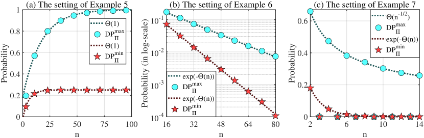
Figure 2: A numerical verification of Theorem 1. Note that the plot for Example 6 is in log-scale.

It is easy to see that the results are consistent with Theorem 1. For example, Figure 2(a) shows that both the max-smoothed likelihood and the min-smoothed likelihood of doctrinal paradoxes are $\Theta(1)$, which matches the result in Table 3. Two additional sets of experiments, whose results are presented in Figure 3(b) in Appendix C, study a more complex setting of three premises.

5 Conclusions and Future Work

We made a first step towards understanding the likelihood of doctrinal paradox in the smoothed analysis framework. There are many immediate open questions. For example, can we characterize the smoothed likelihood of the paradox for general, more complicated propositions (sometimes called agendas)? Can we remove the strict positiveness assumption on $\Pi$? Can we prove smoothed impossibility theorems that extend the quantitative impossibility theorems under i.i.d. uniform distributions [30, 14]? More generally, we believe that building a comprehensive picture of the smoothed properties of aggregation rules in judgement aggregation is a promising (yet challenging) direction in theory and in practice.

Supplementary Material for The Smoothed Likelihood of Doctrinal Paradox

Appendix A Detailed Settings for Section 2 (Preliminary)

A.1 Vectorized indexing for votes or histogram

We fix the judgement of $\vec{\omega}=\vec{\ell}=(\ell_{1},\cdots,\ell_{p})$ to correspond to the $(\overline{\ell_{1}\cdots\ell_{p}}_{(2)}+1)$-th component of $\vec{v}$, where $\overline{\ell_{1}\cdots\ell_{p}}_{(2)}$ is the binary number taking $\ell_{i}$ as the $i$-th digit. For example, if $\omega_{j,1}=1$ and $\omega_{j,2}=0$, we will have $\vec{v}_{j}(\overline{10}_{(2)}+1)=\vec{v}_{j}(3)=1$ while all other components of $\vec{v}_{j}$ are zero.

A.2 Properties of Quota Rules

The properties of quota rules include :
Anonymity: each pair of agents play interchangeable roles.
Neutrality: each pair of propositions are interchangeable.
Independence: the aggregation of a certain proposition only depends on agents’ judgement on this proposition.
Monotonicity: adding vote to the current winner will never change the winner

Appendix B Proof of Theorem 1

Theorem 1 (Smoothed Likelihood for Doctrinal Paradox). Given any strictly positive set $\Pi$ of distributions over $\mathcal{V}$, any logic function $f:\mathcal{V}\to\{0,1\}$, and any quota rule $r$. For any $n\in\mathbb{Z}_{>0}$,

$$\begin{split}&\widetilde{\text{\rm{DP}}}_{\Pi,r,f}^{\max}(n)=\left\{\begin{array}[]{ll}0&\text{if $\kappa_{1}$ is true}\\ \exp(-\Theta(n))&\text{otherwise, if $\kappa_{2}$ is true}\\ \Theta(n^{-1/2})&\text{otherwise, if $\kappa_{4}$ is true}\\ \Theta(1)&\text{otherwise}\\ \end{array}\right.\\ &\widetilde{\text{\rm{DP}}}_{\Pi,r,f}^{\min}(n)=\left\{\begin{array}[]{ll}0&\text{if $\kappa_{1}$ is true}\\ \exp(-\Theta(n))&\text{otherwise, if $\kappa_{3}$ is true}\\ \Theta(n^{-1/2})&\text{otherwise, if $\kappa_{4}$ is true}\\ \Theta(1)&\text{otherwise}\\ \end{array}\right..\end{split}$$

Proof.

We present the full proof for Step 3 discussed in the sketch in the main text.

Step 1: Polyhedra Representation. We prove the following lemma on the connection between $\mathcal{C}$ and the doctrinal paradox.

Lemma 3 (Polyhedra representation of doctrinal paradox).

Given any profile $P\in\mathcal{V}^{n}$ and any distribution $\pi$ on $\mathcal{V}$, any quota rule $r$ and any logical connection function $f$, we have the following two statements for doctrinal paradox,

$$\begin{split}(1)\;\;\;&\forall\,\mathcal{H}\in\mathcal{C},\;\text{\rm Hist}(P)\notin\mathcal{H}\Leftrightarrow\;P\text{ is not a doctrinal paradox}.\\ (2)\;\;\;&\forall\,\mathcal{H}\in\mathcal{C},\;\pi\notin\mathcal{H}_{\leq 0}\Leftrightarrow\;\text{all refinements of $\pi$ are consistent}.\\ \end{split}$$

Proof.

According to the definition of $\mathcal{C}$, we only need to prove the following statement for polyhedra:

Statement 4.

For any profile $P\in\mathcal{V}^{n}$ and any distribution $\pi$ on $\mathcal{V}$, any quota rule $r_{\vec{q},\vec{d}}$ and any logical connection function $f$,

$$\begin{split}\text{\rm Hist}(P)\in\mathcal{H}_{{\vec{\alpha}}}\;\;&\Leftrightarrow\;\;r_{\vec{q},\vec{d}}(P)={\vec{\alpha}}\;\;\;\;\;\;\;\;\;\;\text{and}\\ \pi\in\mathcal{H}_{{\vec{\alpha}},\,\leq 0}\;\;\;\;&\Leftrightarrow\;\;{\vec{\alpha}}\text{ is a refinement of }\pi.\end{split}$$

Let $\vec{\omega}_{\vec{\ell}}$ be the corresponding type of vote when the vote on premises is $\vec{\ell}$. Mathematically, $\vec{\omega}_{\vec{\ell}}\in\mathcal{V}$ and $\vec{\omega}_{\vec{\ell}}(\vec{\ell})=1$. For all $i\in[p+1]$, the characterization vector $\vec{c}_{i}$ can be written as, $\vec{c}_{i}=(q_{i}-1)\cdot\left(\sum_{\vec{\ell}\in\bm{\Omega}_{i}}\vec{\omega}_{\vec{\ell}}\right)+q_{i}\left(\sum_{\vec{\ell}\notin\bm{\Omega}_{i}}\vec{\omega}_{\vec{\ell}}\right)$. Then,

$$\begin{split}\vec{c}_{i}^{\mathsf{T}}\cdot\text{\rm Hist}(P)=\;&\vec{c}_{i}^{\mathsf{T}}\cdot\left(\sum_{\vec{\ell}}\text{\rm Hist}(P)(\vec{\ell})\cdot\vec{\omega}_{\vec{\ell}}\right)\\ =\;&(q_{i}-1)\cdot\left(\sum_{\vec{\ell}\in\bm{\Omega}_{i}}\text{\rm Hist}(P)(\vec{\ell})\right)+q_{i}\left(\sum_{\vec{\ell}\notin\bm{\Omega}_{i}}\text{\rm Hist}(P)(\vec{\ell})\right)\\ =\;&n\cdot q_{i}-\underbrace{\sum_{\vec{\ell}\in\bm{\Omega}_{i}}\text{\rm Hist}(P)(\vec{\ell})}_{\text{number of votes for $\omega_{i}=1$}}.\end{split}$$

According to the definition of quota rule, we know that,

$$\begin{split}\vec{c}_{i}^{\mathsf{T}}\cdot\text{\rm Hist}(P)\leq d_{i}-1\;\;&\Leftrightarrow\;\;r_{\vec{q},\vec{d}}(P)(i)=1\;\;\text{and}\\ -\vec{c}_{i}^{\mathsf{T}}\cdot\text{\rm Hist}(P)\leq-d_{i}\;\;&\Leftrightarrow\;\;r_{\vec{q},\vec{d}}(P)(i)=0\\ \end{split}$$

Then, the first part of Statement 4 follows by the definition of $\mathcal{H}_{{\vec{\alpha}}}$. Follow similar procedure as above, we have,

$$\begin{split}\vec{c}_{i}^{\mathsf{T}}\cdot\pi&=q_{i}-\sum_{\vec{\ell}\in\bm{\Omega}_{i}}\pi(\vec{\ell})\end{split}$$

Thus, for any distribution $\pi$ over $\mathcal{V}$,

$$\begin{split}\vec{c}_{i}^{\mathsf{T}}\cdot\pi\leq 0\;\;&\Leftrightarrow\;\;\exists\,{\vec{\alpha}}\in\mathcal{E}_{\pi}\text{ such that }{\vec{\alpha}}(i)=1\;\;\text{and}\\ -\vec{c}_{i}^{\mathsf{T}}\cdot\pi\leq 0\;\;&\Leftrightarrow\;\;\exists\,{\vec{\alpha}}\in\mathcal{E}_{\pi}\text{ such that }{\vec{\alpha}}(i)=0\\ \end{split}$$

Then, the second part of Statement 4 follows by the definition of $\mathcal{H}_{{\vec{\alpha}},\,\leq 0}$. ∎

Step 2: Apply [42, Theorem 2]. Following [42], for any distribution $\pi$ over $\mathcal{V}$ and any $n\in\mathbb{N}$, the active dimension of $\mathcal{H}$ is formally defined as:

$$\text{dim}_{\mathcal{H},n}(\pi)\triangleq\left\{\begin{array}[]{ll}\text{dim}(\mathcal{H}_{\leq 0})&\text{if }\pi\in\mathcal{H}_{\leq 0}\text{ and }\exists\,P\in\mathcal{V}^{n}\text{ such that }\text{\rm Hist}(P)\in\mathcal{H}\\ -\infty&\text{otherwise }\end{array}\right..$$

We say a polyhedra is active (to $\pi$ at $n$) if and only if $\text{dim}_{\mathcal{H},n}(\pi)\neq-\infty$. In words, an active polyhedron requires (1) there exists a profile of $n$ votes, whose histogram is in the polyhedron, and (2) $\pi$ is in the characteristic cone of the polyhedron. In the next lemma, we reveal a relationship between the active dimensions of polyhedra in $\mathcal{C}$ and the smoothed probability of the doctrinal paradox.

Lemma 5 (Active Dimension$\,\to\,$Smoothed Probability, a direct application of Theorem 2 in [42]).

Given any closed and strictly positive set $\Pi$ of distributions over $\mathcal{V}$, any logical connection function $f:\mathcal{V}\to\{0,1\}$ and any quota rule $r$. For any $n\in\mathbb{N}$,

$$\begin{split}&\widetilde{\text{\rm{DP}}}_{\Pi,r,f}^{\max}(n)=\left\{\begin{array}[]{ll}0&\text{if C1 is true}\\ \exp(-\Theta(n))&\text{otherwise, if C2 is true}\\ \max_{\mathcal{H}\in\mathcal{C}}\Theta\left(n^{(\text{dim}_{\mathcal{H}}(\pi)-m)/2}\right)&\text{otherwise}\\ \end{array}\right.\\ &\widetilde{\text{\rm{DP}}}_{\Pi,r,f}^{\min}(n)=\left\{\begin{array}[]{ll}0&\text{if C1 is true}\\ \exp(-\Theta(n))&\text{otherwise, if C3 is true}\\ \min_{\mathcal{H}\in\mathcal{C}}\Theta\left(n^{(\text{dim}_{\mathcal{H}}(\pi)-m)/2}\right)&\text{otherwise}\\ \end{array}\right.,\\ \end{split}$$

where C1 is: $\forall P\in\mathcal{V}^{n}$, $P$ is not doctrinal paradox.
C2 is: $\forall\,\pi\in\text{CH}(\Pi)\text{ and }\forall\,\mathcal{H}\in\mathcal{C},\;\text{dim}_{\mathcal{H}}(\pi)=-\infty$
C3 is: $\exists\,\pi\in\text{CH}(\Pi)\text{ and }\forall\,\mathcal{H}\in\mathcal{C},\;\text{dim}_{\mathcal{H}}(\pi)=-\infty$.

Note that C1 is the same as $\kappa_{1}$ in Theorem 1. By Lemma 3, we know that $\kappa_{2}$ (or $\kappa_{3}$) is very similar with C2 (or C3), which says that all (or some) distributions in $\text{CH}(\Pi)$ are “far” from all active polyhedra of doctrinal paradoxes.

Step 3: Closing the Gap between Lemma 5 and Theorem 1. The only gap left between Lemma 5 and Theorem 1 is that the active dimension $\text{dim}_{\mathcal{H},n}(\pi)$ is still unknown, which will be characterized in Step 3.1 and 3.2 as follows.

Step 3.1: determine $\text{dim}(\mathcal{H}_{\leq 0})$ (the dimensionality of characteristic cones).

Step 3.1.1: the linear independence of $\{\vec{c}_{1},\cdots,\vec{c}_{p}\}$. We first show that $\vec{c}_{1},\cdots,\vec{c}_{p}$ are linearly independent by contradiction. For any $i\in[p]$, we assume that $\vec{c}_{i}=\sum_{i^{\prime}\neq i}a_{i^{\prime}}\cdot\vec{c}_{i^{\prime}}$, where $a_{i^{\prime}}$ are real valued coefficients. Because $\vec{c}_{i}$ is not a zero vector and different with any $\vec{c}_{i^{\prime}}$, there must exist a pair of $i_{1}^{\prime},i_{2}^{\prime}\in[p]\setminus\{i\}$ such that $a_{i_{1}^{\prime}}\neq 0$ and $a_{i_{2}^{\prime}}\neq 0$. Let $\vec{c}_{i}{(\ell_{1},\ell_{2},\vec{0})}$ to be the coordinate of $\vec{c}_{i}$ corresponds to $\omega_{i_{1}^{\prime}}=\ell_{1}$, $\omega_{i_{2}^{\prime}}=\ell_{2}$ and all other premises are $0$. Because $\vec{c}_{i}$ has the same value in all components that $\omega_{i}=0$. We should have $\vec{c}_{i}{(0,0,\vec{0})}=\vec{c}_{i}{(1,0,\vec{0})}=\vec{c}_{i}{(1,1,\vec{0})}$, which is contradict with the observation that

$$\begin{split}\vec{c}_{i}{(0,0,\vec{0})}&=a_{i_{1}^{\prime}}\cdot q_{i_{1}^{\prime}}+a_{i_{2}^{\prime}}\cdot q_{i_{2}^{\prime}}+\sum_{i^{\prime}\notin\{i_{1}^{\prime}.i_{2}^{\prime}\}}a_{i^{\prime}}\cdot q_{i^{\prime}}\\ \vec{c}_{i}{(1,0,\vec{0})}&=a_{i_{1}^{\prime}}(q_{i_{1}^{\prime}}-1)+a_{i_{2}^{\prime}}\cdot q_{i_{2}^{\prime}}+\sum_{i^{\prime}\notin\{i_{1}^{\prime}.i_{2}^{\prime}\}}a_{i^{\prime}}\cdot q_{i^{\prime}}\\ \vec{c}_{i}{(1,1,\vec{0})}&=a_{i_{1}^{\prime}}(q_{i_{1}^{\prime}}-1)+a_{i_{2}^{\prime}}(q_{i_{2}^{\prime}}-1)+\sum_{i^{\prime}\notin\{i_{1}^{\prime}.i_{2}^{\prime}\}}a_{i^{\prime}}\cdot q_{i^{\prime}}\;\;\;\;\;\;\text{ and thus}\\ \vec{c}_{i}{(0,0,\vec{0})}&-\vec{c}_{i}{(1,0,\vec{0})}=a_{i_{1}^{\prime}}\neq 0\\ \vec{c}_{i}{(1,0,\vec{0})}&-\vec{c}_{i}{(1,1,\vec{0})}=a_{i_{2}^{\prime}}\neq 0.\end{split}$$

Step 3.1.2: the dimension of $\mathcal{H}_{{\vec{\alpha}}}$ when $\kappa_{4}$ is true. When $\kappa_{4}$ is true, the logical connection can be denoted as either $\phi\leftrightarrow\omega_{i}$ or $\phi\leftrightarrow\neg\,\omega_{i}$. For both cases, we have $\text{sign}_{0\to-1}({\alpha}_{p+1})\cdot\vec{c}_{p+1}=-\text{sign}_{0\to-1}({\alpha}_{i})\cdot\vec{c}_{i}$. When $\kappa_{4}$ is true, we will have , the following equation must hold in $\mathcal{H}_{{\vec{\alpha}},\,\leq 0}$.

$$\begin{split}&\vec{x}^{\mathsf{T}}\cdot\left(\text{sign}_{0\to-1}({\alpha}_{p+1})\cdot\vec{c}_{p+1}\right)\\ =\;&\vec{x}^{\mathsf{T}}\cdot\left(\text{sign}_{0\to-1}({\alpha}_{i})\cdot\vec{c}_{i}\right)=0.\end{split}$$

Thus, when $\kappa_{4}$ is not true, we draw the conclusion that

$$\forall\,\mathcal{H}\in\mathcal{C},\;\;\text{dim}(\mathcal{H}_{\leq 0})=m-1\;\;\text{ when $\kappa_{4}$ is true}.$$

Step 3.1.3: the dimension of $\mathcal{H}_{{\vec{\alpha}}}$ when $\kappa_{4}$ is not true. We first show the linear independence between $\vec{c}_{p+1}$ and $\{\vec{c}_{1},\cdots,\vec{c}_{p}\}$ when $\kappa_{4}$ is false. We assume that $\vec{c}_{p+1}=\sum_{i^{\prime}\in[p]}a_{i^{\prime}}\cdot\vec{c}_{i^{\prime}}$, where $a_{i^{\prime}}$ are real valued coefficients. Because $\vec{c}_{p+1}$ is not a zero vector and different with any $\vec{c}_{i^{\prime}}$ when $\kappa_{4}$ is not true, there must exist a pair of $i_{1}^{\prime},i_{2}^{\prime}\in[p]\setminus\{i\}$ such that $a_{i_{1}^{\prime}}\neq 0$ and $a_{i_{2}^{\prime}}\neq 0$. Let $\vec{c}_{p+1}{(\ell_{1},\ell_{2},\vec{0})}$ to be the coordinate of $\vec{c}_{p+1}$ corresponds to $\omega_{i_{1}^{\prime}}=\ell_{1}$, $\omega_{i_{2}^{\prime}}=\ell_{2}$ and all other premises are $0$. Thus, we have the following observations:

$$\begin{split}\vec{c}_{p+1}{(0,0,\vec{0})}&=a_{i_{1}^{\prime}}\cdot q_{i_{1}^{\prime}}+a_{i_{2}^{\prime}}\cdot q_{i_{2}^{\prime}}+\sum_{i^{\prime}\notin\{i_{1}^{\prime}.i_{2}^{\prime}\}}a_{i^{\prime}}\cdot q_{i^{\prime}}\\ \vec{c}_{p+1}{(1,0,\vec{0})}&=a_{i_{1}^{\prime}}(q_{i_{1}^{\prime}}-1)+a_{i_{2}^{\prime}}\cdot q_{i_{2}^{\prime}}+\sum_{i^{\prime}\notin\{i_{1}^{\prime}.i_{2}^{\prime}\}}a_{i^{\prime}}\cdot q_{i^{\prime}}\\ \vec{c}_{p+1}{(1,1,\vec{0})}&=a_{i_{1}^{\prime}}(q_{i_{1}^{\prime}}-1)+a_{i_{2}^{\prime}}(q_{i_{2}^{\prime}}-1)+\sum_{i^{\prime}\notin\{i_{1}^{\prime}.i_{2}^{\prime}\}}a_{i^{\prime}}\cdot q_{i^{\prime}}\;\;\;\;\;\;\text{ and thus}\\ \vec{c}_{p+1}{(0,0,\vec{0})}&-\vec{c}_{p+1}{(1,0,\vec{0})}=a_{i_{1}^{\prime}}\neq 0\\ \vec{c}_{p+1}{(1,0,\vec{0})}&-\vec{c}_{p+1}{(1,1,\vec{0})}=a_{i_{2}^{\prime}}\neq 0.\end{split}$$ (4)

Case 3.1.3.1: $\vec{c}_{p+1}{(0,0,\vec{0})}-\vec{c}_{p+1}{(1,1,\vec{0})}=a_{i_{1}^{\prime}}+a_{i_{2}^{\prime}}\neq 0$. For this case, there must exist at least three different values in $\vec{c}_{i}$, which contradict with the fact that $\vec{c}_{p+1}\in\{q_{p+1}-1,q_{p+1}\}^{m}$.

Case 3.1.3.2: $\vec{c}_{p+1}{(0,0,\vec{0})}-\vec{c}_{p+1}{(1,1,\vec{0})}=a_{i_{1}^{\prime}}+a_{i_{2}^{\prime}}=0$. we note that any nonzero value of $a_{i_{1}^{\prime}}+a_{i_{2}^{\prime}}$ already results in contradiction according to Case 1.1.1. Then, the above relationship of $a_{i_{1}^{\prime}}+a_{i_{2}^{\prime}}=0$ must holds for all nonzero $a_{i^{\prime}}$s, which implies that there cannot exists more than three non-zero values for $a_{i^{\prime}}$. Now, the only case left is $\vec{c}_{i}=a(\vec{c}_{i^{\prime}_{1}}-\vec{c}_{i^{\prime}_{2}})$, where $a$ is a nonzero real number. According to the observations in Inequalities 4, we know that

$$\begin{split}\vec{c}_{p+1}{(0,0,\vec{0})}&=a(q_{i_{1}^{\prime}}-q_{i_{2}^{\prime}})\\ \vec{c}_{p+1}{(1,0,\vec{0})}&=a(q_{i_{1}^{\prime}}-q_{i_{2}^{\prime}}-1)\\ \vec{c}_{p+1}{(0,1,\vec{0})}&=a(q_{i_{1}^{\prime}}-q_{i_{2}^{\prime}}+1),\\ \end{split}$$

which says that $\vec{c}_{p+1}$ has at least three different values and contradict with the fact that $\vec{c}_{p+1}\in\{q_{p+1}-1,q_{p+1}\}^{m}$.

Thus, when $\kappa_{4}$ is not true, we draw the conclusion that

$$\forall\,\mathcal{H}\in\mathcal{C},\;\;\text{dim}(\mathcal{H}_{\leq 0})=m\;\;\text{ when $\kappa_{4}$ is false}.$$

Step 3.2: determine whether the polyhedra is active.
Given the first part of Lemma 3, we know that $\mathcal{H}_{{\vec{\alpha}}}\cap\mathcal{V}^{n}\neq\emptyset$ is equivalent to the statement of “$\exists\,P\in\mathcal{V}^{n}$ such that $r_{\vec{q},\vec{d}}(P)={\vec{\alpha}}$”. Given the first part of Lemma 3, we know that $\pi\in\mathcal{H}_{{\vec{\alpha}},\,\leq 0}$ is equivalent to the statement of “${\vec{\alpha}}$ is a refinement of $\pi$”. Combining the above two statements. We know that polyhedra $\mathcal{H}_{{\vec{\alpha}}}$ is active if and only if ${\vec{\alpha}}$ is an effective refinement of $\pi$. Then, we know that all polyhedra in $\mathcal{C}$ is not active if and only if $\pi$ has no effective refinements of doctrinal paradoxes. Thus, we know that C2 (and C3) in Lemma 5 is equivalent to $\kappa_{2}$ (and $\kappa_{3}$) in Theorem 1. ∎

Appendix C Additional Numerical Results

In Figure 3(b), we present the numerical result for the complex setting introduced in Section 4. The common settings for the two additional experiments are:
Logical connection: conclusion $\phi=1$ if $(\omega_{1},\omega_{2},\omega_{3})\in\{(0,0,0),(0,1,0),(1,1,0)\}$ and $\phi=0$ otherwise.
Breaking criteria: $\vec{d}=(1,0,1,0)$.
Other settings and the results are shown in the Table 5.

Name of setting	Majority	Quota
Threshold $\vec{q}$	$(0.5,0.5,0.5,0.5)$	$(0.2,0.2,0.2,0.2)$
$\widetilde{\text{\rm{DP}}}_{\Pi,r_{\vec{q},\vec{d}},f}^{\max}(n)$	$\exp(-\Theta(n))$	$\Theta(1)$
$\widetilde{\text{\rm{DP}}}_{\Pi,r_{\vec{q},\vec{d}},f}^{\min}(n)$	$\exp(-\Theta(n))$	$\exp(-\Theta(n))$

Table 5: Settings and results for the experiments with three premises

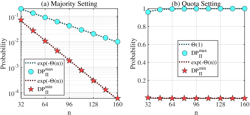
Figure 3: A Numerical verification for the complex setting of three premises. Note that (a) is plotted in log-scale.

In Table 6 - Table 10, we present the expressions of the asymptotic curves under different settings. Root mean square error (RMSE) and coefficient of determination $r^{2}$ shows the fitness between the asymptotic curves and the data points (simulated smoothed probability of doctrinal paradox).

Smoothed Probability	Expressions of the asymptotic curves	RMSE	$r^{2}$
$\widetilde{\text{\rm{DP}}}_{\Pi,r,f}^{\max}(n)$	$1-0.82227\cdot\exp(-0.05941\cdot n)$	$9.850\times 10^{-3}$	$0.99883398$
$\widetilde{\text{\rm{DP}}}_{\Pi,r,f}^{\min}(n)$	$0.25-0.27476\cdot\exp(-0.18796\cdot n)$	$8.337\times 10^{-4}$	$0.99977090$

Table 6: The asymptotic curves in Figure 2(a) for Example 5

Log-Smoothed Probability	Expressions of the asymptotic curves	RMSE	$r^{2}$
$\ln\left(\widetilde{\text{\rm{DP}}}_{\Pi,r,f}^{\max}(n)\right)$	$-0.04904\cdot n-1.0349$	$3.191\times 10^{-2}$	$0.99922895$
$\ln\left(\widetilde{\text{\rm{DP}}}_{\Pi,r,f}^{\min}(n)\right)$	$-0.09964\cdot n-1.0708$	$5.838\times 10^{-2}$	$0.99937469$

Table 7: The asymptotic curves in Figure 2(b) for Example 6

Smoothed Probability	Expressions of the asymptotic curves	RMSE	$r^{2}$
$\widetilde{\text{\rm{DP}}}_{\Pi,r,f}^{\max}(n)$ when $n$ is even	$0.96124\cdot\left(n+0.12519\right)^{-1/2}$	$3.501\times 10^{-3}$	$0.99949065$
$\widetilde{\text{\rm{DP}}}_{\Pi,r,f}^{\min}(n)$ when $n$ is even	$0.65588\cdot\exp(-0.64539\cdot n)$	$7.508\times 10^{-4}$	$0.99989252$

Table 8: The asymptotic curves in Figure 2(c) for Example 7

Smoothed Probability	Expressions of the asymptotic curves	RMSE	$r^{2}$
$\ln\left(\widetilde{\text{\rm{DP}}}_{\Pi,r,f}^{\max}(n)\right)$	$-0.02326\cdot n-0.90777$	$0.01964$	$0.99967488$
$\ln\left(\widetilde{\text{\rm{DP}}}_{\Pi,r,f}^{\min}(n)\right)$	$-0.05555\cdot n-0.94285$	$0.06556$	$0.99936553$

Table 9: The asymptotic curves in Figure 3(a) for the majority setting of three premises

Smoothed Probability	Expressions of the asymptotic curves	RMSE	$r^{2}$
$\widetilde{\text{\rm{DP}}}_{\Pi,r,f}^{\max}(n)$	$1-0.41700\cdot\exp(-0.07436\cdot n)$	$5.528\times 10^{-4}$	$0.99833417$
$\widetilde{\text{\rm{DP}}}_{\Pi,r,f}^{\min}(n)$	$0.25484\cdot\exp(-0.10890\cdot n)$	$1.5780\times 10^{-5}$	$0.99996718$

Table 10: The asymptotic curves in Figure 3(b) for the quota setting of three premises

References

- Awad et al. [2017] Edmond Awad, Richard Booth, Fernando Tohmé, and Iyad Rahwan. Judgement aggregation in multi-agent argumentation. Journal of Logic and Computation, 27(1):227–259, 2017.
- Baharad et al. [2020] Eyal Baharad, Zvika Neeman, and Anna Rubinchik. The rarity of consistent aggregators. Mathematical Social Sciences, 108:146–149, 2020.
- Baumeister et al. [2020] Dorothea Baumeister, Gabor Erdelyi, Olivia J. Erdelyi, Jörg Rothe, and Ann-Kathrin Selker. Complexity of control in judgment aggregation for uniform premise-based quota rules. Journal of Computer and System Sciences, 112:13–33, 2020.
- Bonnefon [2010] Jean-Francois Bonnefon. Behavioral evidence for framing effects in the resolution of the doctrinal paradox. Social Choice and Welfare, 34:631—641, 2010.
- Bonnefon [2011] Jean-Francois Bonnefon. The doctrinal paradox, a new challenge for behavioral psychologists. Advances in Psychological Science, 19(5):617–623, 2011.
- Brandt et al. [2016] Felix Brandt, Vincent Conitzer, Ulle Endriss, Jerome Lang, and Ariel D. Procaccia, editors. Handbook of Computational Social Choice. Cambridge University Press, 2016.
- Chilton and Tingley [2012] Adam Chilton and Dustin Tingley. The doctrinal paradox & international law. University of Pennsylvania Journal of International Law, 34(67), 2012.
- Dietrich and List [2008] Franz Dietrich and Christian List. Judgment aggregation without full rationality. Social Choice and Welfare, 31(1):15–39, 2008.
- Diss and Merlin [2021] Mostapha Diss and Vincent Merlin, editors. Evaluating Voting Systems with Probability Models. Studies in Choice and Welfare. Springer International Publishing, 2021.
- Endriss [2016] Ulle Endriss. Judgment Aggregation. In Handbook of Computational Social Choice, chapter 17. Cambridge University Press, 2016.
- Endriss et al. [2012] Ulle Endriss, Umberto Grandi, and Daniele Porello. Complexity of Judgment Aggregation. Journal of Artificial Intelligence Research, 45:481–514, 2012.
- Endriss et al. [2019] Ulle Endriss, Ronald de Haan, Jerome Lang, and Marija Slavkovik. The Complexity Landscape of Outcome Determination in Judgment Aggregation. Journal of Artificial Intelligence Research, 69:687–731, 2019.
- Everaere et al. [2017] Patricia Everaere, Sebastien Konieczny, and Pierre Marquis. An Introduction to Belief Merging and its Links with Judgment Aggregation. In Trends in Computational Social Choice, chapter 7, pages 123–143. AI Access, 2017.
- Filmus et al. [2020] Yuval Filmus, Noam Lifshitz, Dor Minzer, and Elchanan Mossel. AND testing and robust judgement aggregation. In Proceedings of STOC, 2020.
- Gehrlein and Lepelley [2011] William V. Gehrlein and Dominique Lepelley. Voting Paradoxes and Group Coherence: The Condorcet Efficiency of Voting Rules. Springer, 2011.
- Grossi and Pigozzi [2014] Davide Grossi and Gabriella Pigozzi. Judgment Aggregation: A Primer. Morgan & Claypool Publishers, 2014.
- Hanna [2009] Cheryl Hanna. The paradox of progress: Translating evan stark’s coercive control into legal doctrine for abused women. Violence Against Women, 15(2):1458–1476, 2009.
- Kornhauser and Sager [1986] Lewis A. Kornhauser and Lawrence G. Sager. Unpacking the Court. The Yale Law Journal, 96(1):82–117, 1986.
- Lang and Xia [2016] Jérôme Lang and Lirong Xia. Voting in Combinatorial Domains. In Felix Brandt, Vincent Conitzer, Ulle Endriss, Jérôme Lang, and Ariel Procaccia, editors, Handbook of Computational Social Choice, chapter 9. Cambridge University Press, 2016.
- Lenstra [1983] Hendrik Willem Lenstra. Integer programming with a fixed number of variables. Mathematics of Operations Research, 8:538–548, 1983.
- List [2005] Christian List. The probability of inconsistencies in complex collective decisions. Social Choice and Welfare, 24:3–32, 2005.
- List [2012] Christian List. The theory of judgment aggregation: an introductory review. Synthese, 187:179–207, 2012.
- List and Pettit [2002] Christian List and Philip Pettit. Aggregating sets of judgments: An impossibility result. Economics and philosophy, 18(1):89–110, 2002.
- List and Polak [2010] Christian List and Ben Polak. Introduction to judgment aggregation. Journal of Economic Theory, 145(2):441–466, 2010.
- Lyon and Pacuit [2013] Aidan Lyon and Eric Pacuit. The wisdom of crowds: Methods of human judgement aggregation. In Handbook of human computation, pages 599–614. Springer, 2013.
- Marcoci and Nguyen [2020] Alexandru Marcoci and James Nguyen. Judgement aggregation in scientific collaborations: The case for waiving expertise. Studies in History and Philosophy of Science Part A, 84:66–74, 2020.
- Mongin [2008] Philippe Mongin. Factoring out the impossibility of logical aggregation. Journal of Economic Theory, 141(1):100–113, 2008.
- Mongin [2012] Philippe Mongin. The doctrinal paradox, the discursive dilemma, and logical aggregation theory. Theory and decision, 73(3):315–355, 2012.
- Mongin [2019] Philippe Mongin. The Present and Future of Judgement Aggregation Theory. A Law and Economics Perspective. In The future of economic design, pages 417–429. Springer, 2019.
- Nehama [2013] Ilan Nehama. Approximately classic judgement aggregation. Annals of Mathematics and Artificial Intelligence, 68:91–134, 2013.
- Nehring and Pivato [2021] Klaus Nehring and Marcus Pivato. The median rule in judgement aggregation. Economic Theory, 2021.
- Nehring and Puppe [2008] Klaus Nehring and Clemens Puppe. Consistent judgement aggregation: the truth-functional case. Social Choice and Welfare, 31(1):41–57, 2008.
- Nurmi [1999] Hannu Nurmi. Voting Paradoxes and How to Deal with Them. Springer-Verlag Berlin Heidelberg, 1999.
- Pauly and Hees [2006] Marc Pauly and Martin Van Hees. Logical constraints on judgement aggregation. Journal of Philosophical logic, 35(6):569–585, 2006.
- Pettit [2001] Philip Pettit. Deliberative democracy and the discursive dilemma. Philosophical Issues, 11:268–299, 2001.
- Poisson [1837] Siméon Denis Poisson. Recherches sur la probabilité des jugements en matière criminelle et en matière civile, 1837.
- Rahwan and Tohmé [2010] Iyad Rahwan and Fernando Tohmé. Collective argument evaluation as judgement aggregation. In Proceedings of AAMAS, 2010.
- Sorensen [2003] Roy Sorensen. A Brief History of the Paradox: Philosophy and the Labyrinths of the Mind. Oxford University Press, 2003.
- Spielman and Teng [2009] Daniel A. Spielman and Shang-Hua Teng. Smoothed Analysis: An Attempt to Explain the Behavior of Algorithms in Practice. Communications of the ACM, 52(10):76–84, 2009.
- Vacca [1921] R. Vacca. Opinioni individuali e deliberazioni collettive. Rivista Internazionale di Filosofia del Diritto, 52(52–59), 1921.
- Xia [2020] Lirong Xia. The Smoothed Possibility of Social Choice. In Proceedings of NeurIPS, 2020.
- Xia [2021] Lirong Xia. How Likely Are Large Elections Tied? In Proceedings of ACM EC, 2021.
- Zhang and Conitzer [2019] Hanrui Zhang and Vincent Conitzer. A PAC Framework for Aggregating Agents’ Judgments. In Proceedings of AAAI, 2019.