Abstract

The experimental measurements on flavour physics, in tension with Standard Model predictions, exhibit large sources of Lepton Flavour Universality violation. This note summarises an analysis of the effects of the global fits to the Wilson coefficients assuming a model independent effective Hamiltonian approach, by including a proposal of different scenarios to include the New Physics contributions. Additionally, we include an overview of the impact of the future generation of colliders in the field of $B$-meson anomalies.

Talk presented at the International Workshop on Future Linear Colliders (LCWS2021), 15-18 March 2021. C21-03-15.1.

1 Introduction

In the last few years, several experimental collaborations observed Lepton Flavour Universality Violating (LFUV) processes in $B$ meson decays that would be a clear sign for physics beyond the Standard Model (SM). In the $b\to c\ell\nu$ transitions, signs of violation of lepton universality have been observed in the $e-\tau$, $\mu-\tau$ and $e-\mu$ cases [1, 2, 3]. The $R_{D^{(*)}}^{\ell}$ and $R_{D^{(*)}}^{\mu}$ ratios, defined by,

$$R_{D^{(*)}}^{\ell}=\frac{\mathrm{BR}(B\to D^{(*)}\tau\bar{\nu}_{\tau})}{[\mathrm{BR}(B\to D^{(*)}e\bar{\nu}_{e})+\mathrm{BR}(B\to D^{(*)}\mu\bar{\nu}_{\mu})]/2}\ ,$$ (1)

and

$$R_{D^{(*)}}^{\mu}=\frac{\mathrm{BR}(B\to D^{(*)}\tau\bar{\nu}_{\tau})}{\mathrm{BR}(B\to D^{(*)}\mu\bar{\nu}_{\mu})}\ ,$$ (2)

have received special attention. The measurements of these ratios at BaBar [4], Belle [5] and LHCb [6] experiments are larger than the SM prediction ($R_{D}^{\ell\ \mathrm{SM}}=0.299\pm 0.003$, $R_{D^{*}}^{\ell\ \mathrm{SM}}=R_{D^{*}}^{\mu\ \mathrm{SM}}=0.258\pm 0.005$ [7]). The world average of the experimental values for the $R_{D^{(*)}}$ ratios, as obtained by the Heavy Flavour Averaging Group (HFLAV), assuming universality in the lighter leptons, is [7]

$$R_{D}^{\mathrm{ave}}=0.340\pm 0.027\pm 0.013,\qquad\qquad R_{D^{*}}^{\mathrm{ave}}=0.295\pm 0.011\pm 0.008.$$ (3)

$R_{D}$ exceeds the SM value by $1.4\,\sigma$, and $R_{D^{*}}$ by $2.5\,\sigma$. When combined together, included their correlation, the excess is $3.08\,\sigma$.

Another class of $B$ meson observables showing signs of LFUV is related to $b\to s\ell^{+}\ell^{-}$ processes, namely the optimised angular observable $P_{5}^{\prime}$ [8] and the $R_{K^{(*)}}$ ratios,

$$R_{K^{(*)}}=\frac{\mathrm{BR}(B\to K^{(*)}\mu^{+}\mu^{-})}{\mathrm{BR}(B\to K^{(*)}e^{+}e^{-})}\ .$$ (4)

As a consequence of Lepton Flavour Universality (LFU), $R_{K}=R_{K^{*}}=1$ with uncertainties of the order of $1\%$ in the SM [9, 10]. These ratios are observables that have small theoretical uncertainties. The latest experimental results from LHCb, in the specified regions of $q^{2}$ di-lepton invariant mass, are:

$$R_{K}^{[1.1,6]}=0.846^{+0.042}_{-0.039}{}^{+0.013}_{-0.012}\,\qquad$$ [11]

$$R_{K^{*}}^{[0.045,1.1]}=0.66^{+0.11}_{-0.07}\pm 0.03\qquad\qquad R_{K^{*}}^{[1.1,6]}=0.69^{+0.11}_{-0.07}\pm 0.05\ .\qquad$$ [12] (5)

The compatibility of the individual measurements with respect to the SM predictions is of $3.1\,\sigma$ for the $R_{K}$ ratio, $2.3\,\sigma$ for the $R_{K^{*}}$ ratio in the low-$q^{2}$ region and $2.4\,\sigma$ in the central-$q^{2}$ region. The Belle collaboration has also recently reported experimental results for the $R_{K^{(*)}}$ ratios [13, 14], although with less precision than the LHCb measurements.

A great theoretical effort has been devoted to the understanding of the deviations in the $R_{K^{(*)}}$ and $R_{D^{(*)}}$ observables, and combined explanations for those deviations (see, for example [16, 17, 18, 19, 20, 21, 15, 22, 2, 23, 24, 25, 26, 27, 28, 29, 30, 31, 32, 33, 34, 35, 36, 37, 38, 39, 40, 42, 41] and references therein). Besides, the experimental data has been used to constrain New Physics (NP) models. Several global fits have been performed in the literature [43, 46, 44, 45, 49, 47, 48, 50].

These proceedings are mainly based on our previous work in [15, 50] where we investigate the effects of the global fits to the Wilson coefficients assuming a model independent effective Hamiltonian approach. In section 2 we present a brief summary of the Effective Field Theory used to describe possible NP contributions to $B$ decays observables. A summary of the results obtained in [15] for a fit of the $R_{K^{(*)}}$ ratios and the angular observables $P^{\prime}_{4}$ and $P^{\prime}_{5}$ to the Weak Effective Theory Wilson coefficients is included in this section. Section 3 is devoted to the global fits to the Wilson coefficients, presenting the set of scenarios that we have defined in [50] for the phenomenological study, by considering the NP contributions to the Wilson coefficients in such a way that NP is present in one, two or three of the Wilson coefficients simultaneously. These scenarios are used to study the impact of the global fits to the Wilson coefficients and, therefore, to exhibit more clearly which combinations of Wilson coefficients are preferred and/or constrained by experimental data. We complement our results with a discussion in section 4 of the impact that future $e^{+}e^{-}$ linear colliders will have in the $B$ anomalies [51]. Conclusions are presented in section 5.

2 Effective field theories for $B$ observables

One of the most widely used tools to study any possible New Physics (NP) contribution is the Effective Field Theory. The effective Hamiltonian approach allows us to perform a model-independent analysis of NP effects. In this way, it is possible to obtain constraints on NP contributions to the Wilson coefficients of the Hamiltonian from the experimental results.

The Standard Model Effective Field Theory (SMEFT) is formulated at an energy scale $\mu_{\mathrm{SMEFT}}=\Lambda$ higher that the electroweak (EW) scale, and the degrees of freedom are all SM fields. The Weak Effective Theory (WET) is formulated at an energy scale below the EW scale, for example $\mu_{\mathrm{WET}}=m_{b}$, and the top quark, Higgs, $W$ and $Z$ bosons are integrated out.

The relevant terms of the WET Lagrangian [52, 53, 54] are:

$$\mathcal{L}_{\text{eff}}=-\frac{4G_{F}}{\sqrt{2}}V_{cb}\sum_{\ell=e,\mu,\tau}(1+C_{VL}^{\ell})\mathcal{O}_{VL}^{\ell}+\frac{4G_{F}}{\sqrt{2}}V_{tb}V_{ts}^{*}\frac{e^{2}}{16\pi^{2}}\sum_{\ell=e,\mu}(C_{9}^{\ell}\mathcal{O}_{9}^{\ell}+C_{10}^{\ell}\mathcal{O}_{10}^{\ell})\ ,$$ (6)

where $G_{F}$ is the Fermi constant, $e$ is the electromagnetic coupling, $V_{qq^{\prime}}$ are the elements of the Cabibbo-Kobayashi-Maskawa (CKM) matrix and with the dimension six operators defined as,

$$\mathcal{O}_{VL}^{\ell}=(\bar{c}_{L}\gamma_{\alpha}b_{L})(\bar{\ell}_{L}\gamma^{\alpha}\nu_{\ell})\ ,\qquad\mathcal{O}_{9}^{\ell}=(\bar{s}_{L}\gamma_{\alpha}b_{L})(\bar{\ell}\gamma^{\alpha}\ell)\ ,\qquad\mathcal{O}_{10}^{\ell}=(\bar{s}_{L}\gamma_{\alpha}b_{L})(\bar{\ell}\gamma^{\alpha}\gamma_{5}\ell)\ ,$$ (7)

and their corresponding Wilson coefficients $C_{VL}^{\ell}$, $C_{9}^{\ell}$ and $C_{10}^{\ell}$. The $C_{9}^{\ell}$ and $C_{10}^{\ell}$ Wilson coefficients have contributions from the SM processes as well as any NP contribution,

$$C_{i}^{\ell}=C_{i}^{\mathrm{SM}\,\ell}+C_{i}^{\mathrm{NP}\,\ell}\ ,\qquad\qquad i=9,10\ .$$ (8)

The dependence of the $R_{D^{(*)}}$ ratios on the Wilson coefficients is given by [29, 33]:

$$R_{D^{(*)}}^{\ell} =R_{D^{(*)}}^{\ell,\mathrm{SM}}\frac{|1+C_{VL}^{\tau}|^{2}}{(|1+C_{VL}^{e}|^{2}+|1+C_{VL}^{\mu}|^{2})/2}\ ,$$

$$R_{D^{(*)}}^{\mu} =R_{D^{(*)}}^{\mu,\mathrm{SM}}\frac{|1+C_{VL}^{\tau}|^{2}}{|1+C_{VL}^{\mu}|^{2}}\ .$$ (9)

For the $R_{K^{(*)}}$ ratios, the dependence on the Wilson coefficients has been previously obtained in [15], where an analytic computation of $R_{K^{*0}}$ as a function of $C_{9}^{\rm{NP}\,\mu}$, $C_{10}^{\rm{NP}\,\mu}$ in the region $1.1\leq q^{2}\leq 6.0\,{\rm GeV}^{2}$ was performed. The result is given by [15]:

$$R_{K^{*}}^{[1.1,6]}\simeq\frac{0.9875+0.1759\,\mathrm{Re}\,C_{9}^{\rm{NP}\,\mu}-0.2954\,\mathrm{Re}\,C_{10}^{\rm{NP}\,\mu}+0.0212|C_{9}^{\rm{NP}\,\mu}|^{2}+0.0350|C_{10}^{\rm{NP}\,\mu}|^{2}}{1\,\ \ \ \ \ +0.1760\,\mathrm{Re}\,C_{9}^{\rm{NP}\,e}-0.3013\,\mathrm{Re}\,C_{10}^{\rm{NP}\,e}+0.0212|C_{9}^{\rm{NP}\,e}|^{2}+0.0357|C_{10}^{\rm{NP}\,e}|^{2}}\ .$$ (10)

(a)	(b)

Figure 1: Best fit and $1\sigma$ and $2\sigma$ contours to semi-leptonic $B$-decays observables, $R_{K}$, $R_{K^{*0}}$, $P^{\prime}_{4}$ and $P^{\prime}_{5}$, using (a) real and (b) imaginary Wilson coefficients.

In [15] we performed a fit of the $R_{K^{(*)}}$ ratios and the angular observables $P^{\prime}_{4}$ and $P^{\prime}_{5}$ to the WET Wilson coefficients $C_{9}^{\rm{NP}\,\mu}$and $C_{10}^{\rm{NP}\,\mu}$. We considered two hypothesis: both coefficients being real numbers or imaginary numbers. The allowed regions at $1\,\sigma$ and $2\,\sigma$ are shown in Figure 1. The best fit to the real coefficients is located at $C_{9}^{\rm{NP}\,\mu}=-1.09$, $C_{10}^{\rm{NP}\,\mu}=0.48$ improves the SM predictions by $5.95\,\sigma$, showing a clear preference for non-zero NP contribution to $C_{9}^{\mu}$. The imaginary fit presents two nearly symmetric minima located at $C_{9}^{\rm{NP}\,\mu}=-0.75\,i$, $C_{10}^{\rm{NP}\,\mu}=-0.74\,i$ and $C_{9}^{\rm{NP}\,\mu}=0.72\,i$, $C_{10}^{\rm{NP}\,\mu}=0.74\,i$, with a pull from the SM of $0.9\,\sigma$. In conclusion, purely imaginary Wilson coefficients do not provide a good description of the data. Therefore we will only consider real Wilson coefficients in what follows.

The NP contributions at an energy scale $\Lambda$ ($\Lambda\sim\mathcal{O}(\mathrm{TeV})$) is described by the SMEFT Lagrangian as given in [55],

$$\mathcal{L}_{\mathrm{SMEFT}}=\frac{1}{\Lambda^{2}}\left(C_{\ell q(1)}^{ijkl}\,O_{\ell q(1)}^{ijkl}+C_{\ell q(3)}^{ijkl}\,O^{ijkl}_{\ell q(3)}\right)\ ,$$ (11)

where the dimension six operators are defined as

$$O_{\ell q(1)}^{ijkl}=(\bar{\ell}_{i}\gamma_{\mu}P_{L}\ell_{j})(\bar{q}_{k}\gamma^{\mu}P_{L}q_{l}),\qquad\qquad O_{\ell q(3)}^{ijkl}=(\bar{\ell}_{i}\gamma_{\mu}\tau^{I}P_{L}\ell_{j})(\bar{q}_{k}\gamma^{\mu}\tau^{I}P_{L}q_{l}),$$ (12)

$\ell$ and $q$ are the lepton and quark $SU(2)_{L}$ doublets, $\tau^{I}$ the Pauli matrices, and ${i,j,k,l}$ denote generation indices. The $O_{\ell q(1)}$ operator couples two $SU(2)_{L}$-singlet currents, while the $O_{\ell q(3)}$ operator couples two $SU(2)_{L}$-triplet currents. Consequently, $O_{\ell q(1)}$ only mediates flavour-changing neutral processes, and $O_{\ell q(3)}$ mediates both flavour-changing neutral and charged processes. We will restrict our analysis to operators including only third generation quarks and same-generation leptons, and we will use the following notation for their Wilson coefficients:

$$C_{\ell q}^{e}\equiv C_{\ell q}^{1133}\ ,\qquad\qquad C_{\ell q}^{\mu}\equiv C_{\ell q}^{2233}\ ,\qquad\qquad C_{\ell q}^{\tau}\equiv C_{\ell q}^{3333}\ .$$ (13)

This particular choice of the Wilson coefficients is motivated by the fact that the most prominent discrepancies between SM predictions and experimental measurements, namely $R_{K^{(*)}}$ and $R_{D^{(*)}}$, affect the third quark generation. From a symmetry point of view, this would amount to imposing an $U(2)^{3}=U(2)_{q}\times U(2)_{u}\times U(2)_{d}$ symmetry between the first and second quark generations [56, 57, 58], that remain SM-like. In the lepton sector we only consider diagonal entries in order to avoid Lepton Flavour Violating (LFV) decays.

These operators generate the $C_{VL}^{\ell}$, $C_{9}^{\ell}$ and $C_{10}^{\ell}$ operators of the electroweak effective field theory when matched at the EW scale $\mu_{\mathrm{EW}}$. Using the package wilson [59], we define the $C_{\ell q}$ operators at $\Lambda=1\mathrm{TeV}$, we calculate their running down to $\mu_{\mathrm{EW}}=M_{Z}$, then match them with the EW operators and finally run the down to $\mu=m_{b}$, where the $B$-physics observables are computed. We found the following relations between the Wilson coefficients at high and low energies:

$$C_{9}^{\mathrm{NP}\ e,\mu}=-0.583\,C_{\ell q(1)}^{e,\mu}-0.596\,C_{\ell q(3)}^{e,\mu}\ , \qquad\qquad C_{10}^{\mathrm{NP}\ e,\mu}=0.588\,C_{\ell q(1)}^{e,\mu}+0.591\,C_{\ell q(3)}^{e,\mu}\ ,$$

$$C_{VL}^{e,\mu}=0.0012\,C_{\ell q(1)}^{e,\mu}-0.0644\,C_{\ell q(3)}^{e,\mu}\ , \qquad\qquad C_{VL}^{\tau}=-0.0598\,C_{\ell q(3)}^{\tau}\ .$$ (14)

The $\mathcal{O}_{\ell q}$ operators also produce unwanted contributions to the $B\to K^{(*)}\nu\bar{\nu}$ decays [33, 60]. In order to obey these constraints, we will fix the relation

$$C_{\ell q(1)}^{i}=C_{\ell q(3)}^{i}\equiv C_{\ell q}^{i}\ .$$ (15)

This relation also has the positive consequence of a partial cancellation of loop-induced effects in $Z$-pole and LFV observables.

3 Global fits

The effective operators affect a large number of observables. Therefore, any NP prediction based on Wilson coefficients has to be confronted not only with the $R_{K^{(*)}}$ an $R_{D^{(*)}}$ measurements, but also with additional several measurements involving the decays of $B$ mesons. In the case of the SMEFT, the Renormalization Group evolution produces a mix of the low-energy effective operators and then, modifies the $W$ and $Z$ couplings to leptons. In consequence, NP in the top sector will indirectly affect EW observables, such as the mass of the $W$ boson, the hadronic cross-section of the $Z$ boson $\sigma^{0}_{\mathrm{had}}$ or the branching ratios of the $Z$ to different leptons. In order to keep the predictions consistent with this range of experimental test, global fits have proven to be a valuable tool [46, 45, 47, 48].

In [50] we have performed global fits to the $C_{\ell q}$ Wilson coefficients using the package smelli v1.3 [60]. The global fit includes the $R_{K^{(*)}}$ and $R_{D^{(*)}}$ observables, the $W$ and $Z$ decay widths, the branching ratios to leptons, the $b\to s\mu\mu$ observables (including $P_{5}^{\prime}$ and the branching ratio of $B_{s}\to\mu\mu$) and the $b\to s\nu\bar{\nu}$ observables. The SM input parameters used in the analysis are explicitely given in [50]. They are taken from open source code flavio v1.5 [61], sources used by the program are quoted when available. Concretely, we have supplemented the experimental measurements of the flavio v1.5 database with updated values for $R_{K}$ [11], $R_{D^{(*)}}$ [13], $B\to K^{*}\ell^{+}\ell^{-}$ differential observables [62, 63], $B_{(s)}\to\mu^{+}\mu^{-}$ [64] and a re-analysis of the EW precision tests from LEP [65].

We have defined some specific scenarios, shown in Table 1, for combinations of the $C_{\ell q}^{i}$ operators such that NP contributions to the Wilson coefficients emerge in one, two or three of the Wilson coefficients simultaneously [50]: in Scenarios I-III NP only modifies the $C_{\ell q}$ operators in one lepton flavour at a time; in Scenarios IV-VI NP is present in two of the Wilson coefficients simultaneously; and finally in Scenarios VII-IX we consider the more general case in which three of the $C_{\ell q}^{i}$ operators receive NP contributions. The more general one of these last three scenarios is Scenario VII, in which we consider three independent Wilson coefficients.

The goodness of each fit is evaluated with its difference of $\chi^{2}$ with respect to the SM, $\Delta\chi^{2}_{\mathrm{SM}}=\chi^{2}_{\mathrm{SM}}-\chi^{2}_{\mathrm{fit}}$. The package smelli actually computes the differences of the logarithms of the likelihood function $\Delta\log L=-\frac{1}{2}\Delta\chi^{2}$. In order to compare two fits $A$ and $B$, we use the pull between them in units of $\sigma$, defined as [66, 67]

$$\mathrm{Pull}_{A\to B}=\sqrt{2}\mathrm{Erf}^{-1}[F(\Delta\chi^{2}_{A}-\Delta\chi^{2}_{B};n_{B}-n_{A})]\,,$$ (16)

where $\mathrm{Erf}^{-1}$ is the inverse of the error function, $F$ is the cumulative distribution function of the $\chi^{2}$ distribution and $n$ is the number of degrees of freedom of each fit. We will compare each scenario against two cases: the SM ($C_{\ell q}=0$, $n=0$) and the best fit point using three independent Wilson coefficients (scenario VII). The pull from the SM quantifies how much each scenario is preferred over the SM to describe the data. The larger the pull, the better description of the data of the preferred scenario. The pull of scenario VII quantifies how much the fit over the whole space of parameters is preferred over the simpler and more constrained fits. From the analysis of this pull we are able to discuss the relevance of the proposed scenarios, the larger the pull means that the more restricted scenario represents a worser description of the experimental data.

Scenario		$C_{\ell q}^{e}$	$C_{\ell q}^{\mu}$	$C_{\ell q}^{\tau}$	$\Delta\chi^{2}_{\mathrm{SM}}$	Pull	Pull
						from SM	to VII
I	$e$	$-0.14\pm 0.04$			8.84	2.97 $\sigma$	4.37 $\sigma$
II	$\mu$		$0.10\pm 0.04$		5.47	2.34 $\sigma$	4.73 $\sigma$
III	$\tau$			$-0.38\pm 0.19$	3.85	1.96 $\sigma$	4.89 $\sigma$
IV	$e$ and $\mu$	$-0.25\pm 0.07$	$0.24\pm 0.06$		28.42	4.97 $\sigma$	1.75 $\sigma$
V	$e$ and $\tau$	$-0.14\pm 0.06$		$-0.4\pm 0.3$	12.98	3.17 $\sigma$	4.30 $\sigma$
VI	$\mu$ and $\tau$		$0.10\pm 0.06$	$-0.3\pm 0.3$	8.73	2.49 $\sigma$	4.77 $\sigma$
VII	$e$, $\mu$ and $\tau$	$-0.25\pm 0.02$	$0.211\pm 0.016$	$-0.3\pm 0.4$	31.50	4.97 $\sigma$
VIII	$e=\mu=\tau$	$-0.0139\pm 0.0003$	$-0.0139\pm 0.0003$	$-0.0139\pm 0.0003$	0.30	0.55 $\sigma$	5.23 $\sigma$
IX	$e=-\mu=\tau$	$-0.232\pm 0.001$	$0.232\pm 0.001$	$-0.232\pm 0.001$	30.74	5.54 $\sigma$	0.41 $\sigma$

Table 1: Best fit values and pulls from the Standard Model and of scenario VII for several combinations of $C_{\ell q}^{i}$ operators.

The results of the fits are summarised in Table 1 for several combinations of $C_{\ell q}^{i}$ operators, with one, two or three lepton flavour present simultaneously in the Wilson coefficients. The best fit values at 1 $\sigma$ and pulls from the SM and to scenario VII for all cases are included in this table.

Summarising the results, we found that the largest pull from the SM prediction when NP only modifies the $C_{\ell q}^{i}$ operators in one lepton flavour at a time, i.e $C_{\ell q}^{e}$, $C_{\ell q}^{\mu}$ or $C_{\ell q}^{\tau}$, is obtained in scenario I where the coupling to electrons is added. It is almost $3\ \sigma$. This result is a reflection of the great impact of the EW precision observables in the global fit. If we restricted our fit to only $b\to s\ell^{+}\ell^{-}$ observables, the fit to only muons in scenario II would display a better pull from the SM of $2.34\ \sigma$, in line with the common wisdom about the anomalies, explaining them through NP in the muon sector [19, 21, 43, 66, 68]. The worst pull is obtained in the fit to the tau coefficient, with $1.96\ \sigma$, as it does not modify the value of the $R_{K^{(*)}}$ ratios. On the other hand, scenarios I and II both produce SM-like predictions for the observables $R_{D}$ and $R_{D^{*}}$. Scenario III, with a larger value of its Wilson coefficient, produces values closer to the experimental measurements; i.e $R^{\ell}_{D}=0.318$ and $R^{\ell}_{D^{*}}=0.268$. In order to fully address the anomaly in these observables, a larger deviation from the SM would be needed; however such a deviation would be in conflict with the EW precision data, as we obtained in [50], and in agreement with [69].

For the scenario in which NP is present in two of the Wilson coefficients, the best fit corresponds to scenario IV, where the contributions to $C_{\ell q}^{e}$ and $C_{\ell q}^{\mu}$ are favoured with a pull of $4.97\ \sigma$ with respect to the SM. Figure 2 shows the allowed regions for these fits. In the fit to Scenario IV, the $R_{K^{(*)}}$ and $R_{D^{(*)}}$ observables constrain the $C_{\ell q}^{e}-C_{\ell q}^{\mu}$ combination; while the LFU-conserving EW precision observables tightly constrain the combination $C_{\ell q}^{e}+C_{\ell q}^{\mu}$. Clearly, the EW precision observables play an important role in the global fit and the preferred values for the Wilson coefficients. The reason for this behaviour is justified by deviations in $Z$-couplings to leptons, the $\tau$-leptonic decays and the Z and W decays widths, as shown in [70]. The values of the $R_{K^{(*)}}$ and $R_{D^{(*)}}$ observables in this scenario are given in Table 2. Together, these sets of observables constrain the fit to a narrow ellipse around the best fit point. In Scenarios V and VI, the $C_{\ell q}^{\tau}$ coefficient is determined by the EW precision observables, that are compatible with a SM-like coefficient, and by $R_{D^{(*)}}$ observables, that prefer a large negative value. All the experimental constraints for $C_{\ell q}^{\tau}$ show large uncertainties, which result in less statistical significance of these fits and $C_{\ell q}^{\tau}$ still being compatible with zero at $2\,\sigma$ level.

(a)	(b)	(c)

Figure 2: $1\sigma$ and $2\sigma$ contours for scenarios with two lepton flavours present in the Wilson coefficients: (a) Scenario IV, (b) Scenario V, and (c) Scenario VI. All available data are considered.

As already established, the more general cases are the ones in which three of the $C_{\ell q}^{i}$ operators receive NP contributions. A particular scenario corresponds with universal couplings (Scenario VIII); i.e the three Wilson coefficients have the same universal contribution, and does not violate LFU. We found the smallest pull with respect to the SM ($0.55\,\sigma$) in this case, which shows that LFU NP can not explain experimental data and, therefore, LFU violation is needed to accommodate it. When the three $C_{\ell q}$ operators receive independent NP contribution (Scenario VII), the pull from the SM, $4.97\ \sigma$, is similar to that of scenario IV, and the values of $C_{\ell q}^{e}$ and $C_{\ell q}^{\mu}$ are similar too, therefore the predictions for the $R_{K^{(*)}}$ observables are very similar, as shown in Figure 3a. The value of $C_{\ell q}^{\tau}$ is close to that of Scenarios III, V and VI, which allows a best fit to the $R_{D^{(*)}}$ observables, and especially to $R_{D}^{\ell}$, that is compatible at $1\,\sigma$ with its experimental value, as shown in Figure 3b. Therefore, we conclude that the prediction of the $R_{D^{(*)}}$ observables is improved in scenario VII. This scenario was analysed in more detail in [50]. We found that the constraints to the fit can be explained by the combined effect of three different classes of observables: in the first place, the linear combination $C_{3}\sim(-C_{\ell q}^{e}+C_{\ell q}^{\mu})/\sqrt{2}$ shows a clear preference for a LFU-violating situation, driven mostly by $R_{K}$ and $R_{K^{*}}$, and in tension with $\mathrm{BR}(\pi^{+}\to e\nu)$, $R_{D^{*}}^{e/\mu}$ and $R_{e\mu}(K^{+}\to\ell^{+}\nu)$. The second class of observables are LFU-conserving, affecting the linear combination $C_{2}\sim(-C_{\ell q}^{e}-C_{\ell q}^{\mu})/\sqrt{2}$, the more relevant observables being the EW precision tests (the mass of the $W$ boson $m_{W}$, the $Z$-decay asymmetries $A_{e}$, $A_{\tau}$ and $A_{\mathrm{FB}}$ and the $Z$ decay width $\Gamma_{Z}$). Our fit is less sensitive to the third class of observables, those that affect $\tau$ physics in $C_{1}\sim-C_{\ell q}^{\tau}$, where the more relevant constraints come from the leptonic decays $\tau\to e\bar{\nu}\nu$ and $\tau\to\mu\bar{\nu}\nu$, the hadronic cross-section of the $Z$ $\sigma^{0}_{\mathrm{had}}$, and the ratios $R_{D^{(*)}}$. The LFU-violating observables, as well as the $\tau\to e\bar{\nu}\nu$ decay, proved to be the most relevant observables in the fit overall. Finally, Scenario IX corresponds with the three Wilson coefficients having the same absolute value, but $C_{\ell q}^{\mu}$ has the opposite sign. This particular arrangement of the coefficients was inspired by the similar absolute values of $C_{\ell q}^{e}$ and $C_{\ell q}^{\mu}$ in Scenario VII. This choice produces a good fit, with a pull of $5.54\,\sigma$. It is also the only scenario that remains compatible at $1\,\sigma$ with scenario VII.

Observable	Scenario IV	Scenario VII	Scenario IX	Measurement
$R_{K}^{[1.1,6]}$	$0.799\pm 0.017$	$0.800\pm 0.018$	$0.79\pm 0.02$	$0.85\pm 0.04$
$R_{K^{*}}^{[0.045,\ 1.1]}$	$0.870\pm 0.009$	$0.871\pm 0.010$	$0.870\pm 0.010$	$0.65\pm 0.09$
$R_{K^{*}}^{[1.1,\ 6]}$	$0.800\pm 0.018$	$0.802\pm 0.019$	$0.80\pm 0.02$	$0.68\pm 0.10$
$R_{D}^{\ell}$	$0.302\pm 0.005$	$0.314\pm 0.007$	$0.311\pm 0.005$	$0.35\pm 0.03$
$R_{D^{*}}^{\ell}$	$0.254\pm 0.004$	$0.264\pm 0.004$	$0.261\pm 0.004$	$0.296\pm 0.016$
$R_{D^{*}}^{\mu}$	$0.261\pm 0.004$	$0.272\pm 0.004$	$0.269\pm 0.004$	$0.31\pm 0.03$

Table 2: Values of the $R_{K^{(*)}}$ and $R_{D^{(*)}}$ observables in the scenarios with best pulls.

The results for the $R_{K^{(*)}}$ and $R_{D^{(*)}}$ observables in the scenarios with best pulls, Scenarios IV, VII and IX, are presented in Table 2. For comparison, an statistical combination of all the available measurements of each observable, performed by flavio is included in the last column of this table. In the case of the $R_{D^{(*)}}$ ratios, this combination does not assume flavour universality between electrons and muons. Figure 3 shows the results for the central value and $1\,\sigma$ uncertainty of these two observables in the three scenarios, compared to the SM prediction (yellow area) and experimental measurements (green area). These three scenarios have similar fits for the Wilson coefficients $C_{\ell q}^{e}$ and $C_{\ell q}^{\mu}$, and therefore reproduce the experimental value of $R_{K}^{[1.1,6]}$ and reduce the tension in $R_{K^{*}}^{[1.1,6]}$. The main difference between Scenarios IV, VII and IX is the fit for $C_{\ell q}^{\tau}$: Scenario IV has no NP contribution in the $\tau$ sector and consequently predicts SM-like $R_{D^{(*)}}$ ratios. Scenario VII has a large contribution to $C_{\ell q}^{\tau}$ and is able to produce a prediction for $R_{D}^{\ell}$ compatible with the experimental results, and significantly improve the predictions for $R_{D^{*}}^{\ell}$ and $R_{D^{*}}^{\mu}$. Scenario IX has an intermediate value of $C_{\ell q}^{\tau}$, and consequently its predictions for the $R_{D^{(*)}}$ ratios are not as good as in Scenario VII.

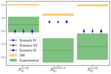
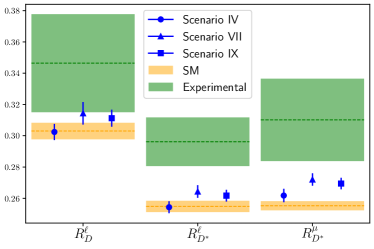
(a)	(b)

Figure 3: Central value and $1\sigma$ uncertainty of the (a) $R_{K^{(*)}}$ observables, and (b) $R_{D^{(*)}}$ observables (blue lines) in scenarios IV, VII and IX, compared to the SM prediction (yellow) and experimental measurements (green).

In addition to the observables included in our global fits, it is also possible to constrain the NP contributions to Wilson coefficients using high-energy collision data from LHC [71, 72]. We also have checked that all the results of our fits are compatible with the limits imposed by the high-$p_{T}$ phenomena [50].

4 Prospects from $e^{+}e^{-}$ colliders

A new generation of particle colliders, complementary to the LHC and its upgrade HL-LHC, will be ready in the coming decades. The International Linear Collider (ILC) will be a linear $e^{+}e^{-}$ collider in Japan, operating at center-of-mass energies ranging from $\sqrt{s}=$250 GeV at the first stages up to $\sqrt{s}=$1 TeV [73]. The Compact Linear Collider (CLIC) at CERN will also be a linear $e^{+}e^{-}$ collider, operating from $\sqrt{s}=$ 380 GeV up to $\sqrt{s}=$ 3 TeV [74]. The Future Circular Collider (FCC), also at CERN, will be a circular collider first using electrons (FCC-ee) from $\sqrt{s}=$90 GeV ($Z$ pole) up to $\sqrt{s}=$365 GeV, and then using hadrons (FCC-hh) reaching $\sqrt{s}=$100 TeV [75]. These colliders are conceived primarily as Higgs factories, exploring the origin of the electroweak symmetry breaking mechanism and the hierarchy problem. But they can also supplement the flavour programs of the LHCb and Belle in different ways: by producing $b$-flavoured hadrons in $e^{+}e^{-}\to Z\to b\overline{b}$ events (ILC operating at the $Z$ pole is expected to produce around $10^{9}$ $Z$s (“GigaZ”) [76], and the FCC-ee is expected to deliver $10^{12}$ $Z$s (“TeraZ”) [77]); by searching for new particles responsible for the deviations, such as leptoquarks or $Z^{\prime}$ bosons; by probing the effects of Wilson coefficients in the kinematical distributions sensible to virtual effects; and by improving the precision of the observables that enter our global fits. Due to the high number of $Z$ bosons produced, EW observables are a prime example of the advantages of $e^{+}e^{-}$ colliders.

In what follows, we will focus on the prospects of indirect discovery using Wilson coefficients and EW observables. The increased center-of-mass energy of the future colliders improves the sensitivity to the effects of any dimension-6 Wilson coefficient. This is evident from the energy scaling of the $2\to 2$ scattering amplitudes, $A_{6}\propto\frac{E^{2}}{\Lambda^{2}}\,$ [78].

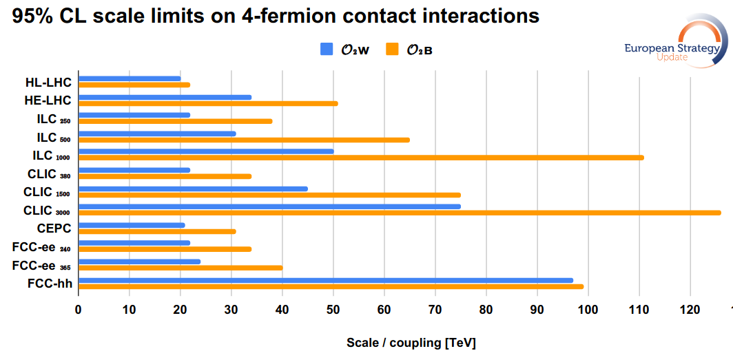
Figure 4: 95% exclusion reach in future colliders from the operators $\mathcal{O}_{2W}$ (blue) and $\mathcal{O}_{2B}$ (orange). The effective scale is given by $\Lambda/({g^{\prime}}^{2}\sqrt{C_{2W}})$ for the blue bars, and $\Lambda/(g^{2}\sqrt{C_{2B}})$ for the orange bars. Taken from [81].

The study of neutral-current benefits greatly from the clean signatures and small theoretical uncertainties provided by lepton colliders. The use of polarized beams allows for the study of the different helicity structures of the Wilson coefficients. The constraints from lepton colliders for the four-fermion contact operators are the result of a variety of final states. For example, the $e^{+}e^{-}\to t\overline{t}$ events can constrain $C_{\ell q(1)}-C_{\ell q(3)}$, while $e^{+}e^{-}\to b\overline{b}$ events can constrain $C_{\ell q(1)}+C_{\ell q(3)}$ [79]. Also the leading higher-derivative corrections to the $W$ and $Z$ bosons propagators from the $\mathcal{O}_{2W}$ and $\mathcal{O}_{2B}$ operators,

$$\mathcal{O}_{2W}=(D^{\mu}W_{\mu\nu})^{i}(D_{\rho}W^{\rho\nu})^{i},\qquad\qquad\mathcal{O}_{2B}=(\partial^{\mu}B_{\mu\nu})(\partial_{\rho}B^{\rho\nu})$$ (17)

from the Strongly-Interacting Light Higgs (SILH) basis [80] can be recast into flavour-universal four-fermion operators using the equations of motion

$$\mathcal{O}_{2W}=-\frac{g^{2}}{4}\sum_{i,j}O_{\ell q(3)}^{iijj}+\cdots,\qquad\qquad\mathcal{O}_{2B}=-\frac{{g^{\prime}}^{2}}{6}\sum_{i,j}O_{\ell q(1)}^{iijj}+\cdots,$$ (18)

where $g$ and $g^{\prime}$ are the gauge couplings for the $SU(2)_{L}$ and $U(1)_{Y}$ SM groups.

The exclusion reach for the operators $\mathcal{O}_{2W}$ and $\mathcal{O}_{2B}$ in the different colliders are depicted in Figure 4, taken from [81]. Lepton colliders provide better sensitivity for singlet operators ($\mathcal{O}_{2B}$) than for triplet operators ($\mathcal{O}_{2W}$), while the sensitivity of hadron colliders is similar in both cases. In its initial stage at $\sqrt{s}=$250 GeV, ILC is expected to provide a better sensitivity than the high-luminosity upgrade of LHC.

An important feature of our model is that it predicts NP couplings to electrons similar in magnitude to the couplings to muons. This opens the option of observation in an $e^{+}e^{-}$ machine, specially using $e^{+}e^{-}\to bs$ production, which has a very clean SM background, since this process is only generated at one loop and CKM-suppressed by $V_{ts}$ [82].

The lepton linear colliders running at their initial stages will generate a great number of $W$ and $Z$ bosons (about $10^{8}$ in ILC at $\sqrt{s}=$ 250 GeV and $10^{7}$ in CLIC at $\sqrt{s}=$ 380 GeV [81]). This will allow to improve the precision of the EW observables: the mass of the $W$ boson $m_{W}$, and the decay asymmetries $A$ and rates $R$ of the $Z$ boson. A dedicated program running at the $Z$ pole would increase the number of bosons by an order of magnitude, improving accordingly the precision of the measurements. Circular $e^{+}e^{-}$ colliders using transversely polarised beams will achieve even better results.

In our fits in section 3 we have shown that the EW observables, due to the mixing via Renormalization Group Equations, offer a set of constraints on NP complementary to those coming from $B$ decays. A significant improvement in the precision of EW observables would have consequently a great impact on our results. In order to asses the impact of the improved precision on our previous analysis, we have performed a new global fit [51] . For the central values of the EW observables we have used their predictions in our previous fits [50], and the uncertainty is taken from the ILC at $\sqrt{s}=$ 250 GeV projections from [81]. The assumed values of the central EW observables and their uncertainties are shown on Table 3. The other observables are unchanged since our previous work [50]. The largest tensions between our inputs and the SM predictions are found in the observables $A_{e}$ and $m_{W}$, being $5.6\,\sigma$ and $2.9\,\sigma$ respectively.

Obs	Central value					Error
	IV	V	VI	VII	IX
$m_{W}$ [GeV]	80.363	80.382	80.342	80.365	80.359	0.002
$A_{e}$	0.14779	0.14900	0.14580	0.14785	0.14738	0.00015
$A_{\mu}$	0.1471	0.1488	0.1457	0.14716	0.1467	0.0008
$A_{\tau}$	0.1474	0.1494	0.1463	0.14798	0.1474	0.0008
$A_{c}$	0.6677	0.6683	0.6670	0.6677	0.6675	0.0014
$A_{b}$	0.9347	0.9349	0.9346	0.9348	0.9347	0.0006
$R_{e}$	20.73	20.73	20.73	20.73	20.73	0.02
$R_{\mu}$	20.74	20.74	20.74	20.74	20.74	0.02
$R_{\tau}$	20.78	20.77	20.77	20.77	20.77	0.02
$R_{c}$	0.1722	0.1722	0.1722	0.1722	0.1722	0.0008
$R_{b}$	0.2158	0.2158	0.2158	0.2158	0.2158	0.0002

Table 3: Assumed central values for the EW observables and their uncertainties used in the ILC global fits for several scenarios.

(a)	(b)	(c)

Figure 5: Detail of the $1\sigma$ and $2\sigma$ contours for scenarios with two lepton flavours present in the Wilson coefficients: (a) Scenario IV, (b) Scenario V, and (c) Scenario VI. Solid lines correspond to the current fits, and dash-dotted lines to the fits including the ILC projections.

The fits to scenarios IV, V and VI using the projected ILC values are already included in Figure 2. For clarification, a detailed region in which the ILC prediction appears is displayed in Figure 5. The LFU-conserving direction of the fit, corresponding to the linear combination $C_{2}\sim(-C_{\ell q}^{e}-C_{\ell q}^{\mu})/\sqrt{2}$, is even more tightly constrained due to the better precision of the EW observables, obtaining $C_{2}=-0.034\pm 0.011$ in scenario VII. The LFUV direction of the fit remains unchanged, since the EW observables are not sensitive to these deviations.

Observable	Scenario IV	Scenario VII	Scenario IX
$R_{K}^{[1.1,6]}$	$0.802\pm 0.003$	$0.803\pm 0.005$	$0.807\pm 0.004$
$R_{K^{*}}^{[0.045,\ 1.1]}$	$0.872\pm 0.004$	$0.872\pm 0.008$	$0.873\pm 0.009$
$R_{K^{*}}^{[1.1,\ 6]}$	$0.804\pm 0.005$	$0.805\pm 0.006$	$0.809\pm 0.008$
$R_{D}^{\ell}$	$0.302\pm 0.005$	$0.309\pm 0.005$	$0.310\pm 0.005$
$R_{D^{*}}^{\ell}$	$0.254\pm 0.003$	$0.260\pm 0.003$	$0.261\pm 0.004$
$R_{D^{*}}^{\mu}$	$0.262\pm 0.003$	$0.267\pm 0.004$	$0.269\pm 0.004$

Table 4: Values of the $R_{K^{(*)}}$ and $R_{D^{(*)}}$ observables in the scenarios with better pulls for the fit with the upgraded ILC precision.

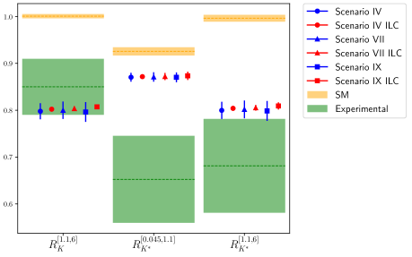
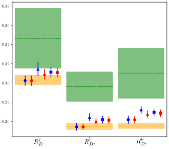
(a)	(b)

Figure 6: Central value and $1\sigma$ uncertainty of the (a) $R_{K^{(*)}}$ observables, and (b) $R_{D^{(*)}}$ observables in scenarios IV, VII and IX (blue lines for current predictions, red lines for ILC-based predictions), compared to the SM prediction (yellow) and experimental measurements (green).

The predictions for the $R_{K^{(*)}}$ and $R_{D^{(*)}}$ observables in the best fit points for scenarios IV, VII and IX with the upgraded ILC precision can be found in Table 4. Clearly, the precision in all those observables is improved. To compare with our previous fit, Figure 6 displays the central value and $1\sigma$ uncertainty of the $R_{K^{(*)}}$ and $R_{D^{(*)}}$ observables in the above mentioned scenarios for the current predictions (blue lines) and the ILC predictions (red lines). The error in all those observables is now dominated by the theoretical uncertainty, as a consequence of the reduction of the allowed region for the Wilson coefficients in the fits. The error of the $R_{K^{(*)}}$ observables is improved up to factor of 3, specially in the $1.1<q^{2}<6$ region, in which the results of the global fits are in agreement with the experimental measurements.

5 Conclusions

Several measurements of $B$ meson decays performed in the recent years indicate a possible violation of Lepton Universality that may represent an indirect signal of New Physics. In this note we summarise the results obtained in [15, 50] for the analysis of the effects of the global fits to the Wilson coefficients assuming a model independent effective Hamiltonian approach. The global fit includes $b\to s\mu\mu$ observables (including the Lepton Flavour Universality ratios $R_{K^{(*)}}$, the angular observables $P_{5}^{\prime}$ and the branching ratio of $B_{s}\to\mu\mu$), as well as the $R_{D^{(*)}}$, $b\to s\nu\bar{\nu}$ and electroweak precision observables ($W$ and $Z$ decay widths and branching ratios to leptons).

We consider different scenarios for the phenomenological analysis such that New Physics is present in one, two or three of the Wilson coefficients at a time. For all scenarios we compare the results of the global fit with respect to both the SM and the more general scenario: the best fit point of the three independent Wilson coefficients scenario in which New Physics modifies each of the operators independently.

We conclude that, when New Physics contributes to only one lepton flavour operator at a time, the largest pull from the Standard Model prediction, almost $3\ \sigma$, appears when the coupling to electrons is added independently, corresponding to our scenario I. In those scenarios in which New Physics is present in two of the Wilson coefficients simultaneously, the best fit corresponds to the case of scenario IV, where the contributions to $C_{\ell q}^{e}$ and $C_{\ell q}^{\mu}$ are favoured with a pull of $4.97\ \sigma$ with respect to the SM. If we focus on the more general scenario of three independent Wilson coefficients, we found that the prediction of the $R_{D^{(*)}}$ and $R_{K^{(*)}}$ observables is improved in the scenario in which the three $C_{\ell q}$ operators receive independent NP contributions: Scenario VII. In this case, the pull from the Standard Model is $4.97\ \sigma$ and the predictions for the $R_{K^{(*)}}$ observables are very similar to the case of Scenario IV. A better fit to $R_{D^{(*)}}$ observables, and specially to $R_{D}^{\ell}$, is obtained in this scenario. We also found that Scenario IX provides a similar fit goodness with a smaller set of free parameters.

Finally, we have discussed that the future particle colliders, and in particular the linear lepton colliders ILC and CLIC, will provide valuable new information to cast light on the $B$ anomalies. For the $R_{K^{(*)}}$ observables, the error is improved up to factor of 3, specially in the $1.1<q^{2}<6$ region, in which the results of the global fits are in agreement with the experimental measurements. Improved precision in electroweak observables will help constrain the global fits in a complementary way to $B$-physics experiments.

References

- [1] A. Abdesselam et al. [Belle Collaboration], [arXiv:1702.01521 [hep-ex]].
- [2] M. Jung and D. M. Straub, JHEP 01 (2019), 009 doi:10.1007/JHEP01(2019)009 [arXiv:1801.01112 [hep-ph]].
- [3] C. Bobeth, D. van Dyk, M. Bordone, M. Jung and N. Gubernari, [arXiv:2104.02094 [hep-ph]].
- [4] J. P. Lees et al. [BaBar], Phys. Rev. Lett. 109 (2012), 101802 doi:10.1103/PhysRevLett.109.101802 [arxiv:1205.5442 [hep-ex]].
- [5] A. Abdesselam et al. [Belle Collaboration], [arXiv:1904.08794 [hep-ex]].
- [6] R. Aaij et al. [LHCb Collaboration], Phys. Rev. Lett. 120 (2018) no.17, 171802 doi:10.1103/PhysRevLett.120.171802 [arXiv:1708.08856 [hep-ex]].
- [7] Y. S. Amhis et al. [HFLAV Collaboration], Eur. Phys. J. C 81 (2021) no.3, 226 doi:10.1140/epjc/s10052-020-8156-7 [arXiv:1909.12524 [hep-ex]].
- [8] S. Descotes-Genon, J. Matias, M. Ramon and J. Virto, JHEP 01 (2013), 048 doi:10.1007/JHEP01(2013)048 [arXiv:1207.2753 [hep-ph]].
- [9] G. Hiller and F. Kruger, Phys. Rev. D 69 (2004), 074020 doi:10.1103/PhysRevD.69.074020 [arXiv:hep-ph/0310219 [hep-ph]].
- [10] M. Bordone, G. Isidori and A. Pattori, Eur. Phys. J. C 76 (2016) no.8, 440 doi:10.1140/epjc/s10052-016-4274-7 [arXiv:1605.07633 [hep-ph]].
- [11] R. Aaij et al. [LHCb Collaboration], [arXiv:2103.11769 [hep-ex]].
- [12] R. Aaij et al. [LHCb Collaboration], JHEP 1708 (2017) 055 doi:10.1007/JHEP08(2017)055 [arXiv:1705.05802 [hep-ex]].
- [13] S. Choudhury et al. [Belle Collaboration], JHEP 03 (2021), 105 doi:10.1007/JHEP03(2021)105 [arXiv:1908.01848 [hep-ex]].
- [14] A. Abdesselam et al. [Belle Collaboration], Phys. Rev. Lett. 126 (2021) no.16, 161801 doi:10.1103/PhysRevLett.126.161801 [arXiv:1904.02440 [hep-ex]].
- [15] J. Alda, J. Guasch and S. Peñaranda, Eur. Phys. J. C 79 (2019) no.7, 588 doi:10.1140/epjc/s10052-019-7092-x [arXiv:1805.03636 [hep-ph]].
- [16] W. Altmannshofer, C. Niehoff, P. Stangl and D. M. Straub, Eur. Phys. J. C 77 (2017) no.6, 377 doi:10.1140/epjc/s10052-017-4952-0 [arXiv:1703.09189 [hep-ph]].
- [17] G. Hiller and M. Schmaltz, JHEP 1502 (2015) 055 doi:10.1007/JHEP02(2015)055 [arXiv:1411.4773 [hep-ph]]; G. Hiller and I. Nisandzic, Phys. Rev. D 96 (2017) no.3, 035003 doi:10.1103/PhysRevD.96.035003 [arXiv:1704.05444 [hep-ph]].
- [18] T. Hurth, F. Mahmoudi and S. Neshatpour, Nucl. Phys. B 909 (2016) 737 doi:10.1016/j.nuclphysb.2016.05.022 [arXiv:1603.00865 [hep-ph]].
- [19] W. Altmannshofer, P. Stangl and D. M. Straub, Phys. Rev. D 96 (2017) no.5, 055008 doi:10.1103/PhysRevD.96.055008 [arXiv:1704.05435 [hep-ph]].
- [20] L. S. Geng et al., Phys. Rev. D 96 (2017) no.9, 093006 doi:10.1103/PhysRevD.96.093006 [arXiv:1704.05446 [hep-ph]].
- [21] M. Ciuchini et al., Eur. Phys. J. C 77 (2017) no.10, 688 doi:10.1140/epjc/s10052-017-5270-2 [arXiv:1704.05447 [hep-ph]].
- [22] A. K. Alok, D. Kumar, J. Kumar, S. Kumbhakar and S. U. Sankar, JHEP 09 (2018), 152 doi:10.1007/JHEP09(2018)152 [arXiv:1710.04127 [hep-ph]].
- [23] S. Bhattacharya, S. Nandi and S. Kumar Patra, Eur. Phys. J. C 79 (2019) no.3, 268 doi:10.1140/epjc/s10052-019-6767-7 [arXiv:1805.08222 [hep-ph]].
- [24] C. Murgui, A. Peñuelas, M. Jung and A. Pich, JHEP 09 (2019), 103 doi:10.1007/JHEP09(2019)103 [arXiv:1904.09311 [hep-ph]].
- [25] M. Blanke et al., Phys. Rev. D 100 (2019) no.3, 035035 doi:10.1103/PhysRevD.100.035035 [arXiv:1905.08253 [hep-ph]].
- [26] B. Bhattacharya, A. Datta, D. London and S. Shivashankara, Phys. Lett. B 742 (2015), 370-374 doi:10.1016/j.physletb.2015.02.011 [arXiv:1412.7164 [hep-ph]].
- [27] L. Calibbi, A. Crivellin and T. Ota, Phys. Rev. Lett. 115 (2015), 181801 doi:10.1103/PhysRevLett.115.181801 [arXiv:1506.02661 [hep-ph]]; L. Calibbi, A. Crivellin and T. Li, Phys. Rev. D 98 (2018) no.11, 115002 doi:10.1103/PhysRevD.98.115002 [arXiv:1709.00692 [hep-ph]].
- [28] G. Hiller, D. Loose and K. Schönwald, JHEP 12 (2016), 027 doi:10.1007/JHEP12(2016)027 [arXiv:1609.08895 [hep-ph]].
- [29] B. Bhattacharya, A. Datta, J. P. Guévin, D. London and R. Watanabe, JHEP 01, 015 (2017) doi:10.1007/JHEP01(2017)015 [arXiv:1609.09078 [hep-ph]].
- [30] A. Crivellin, D. Müller and T. Ota, JHEP 09 (2017), 040 doi:10.1007/JHEP09(2017)040 [arXiv:1703.09226 [hep-ph]]; A. Crivellin, D. Müller and F. Saturnino, JHEP 06 (2020), 020 doi:10.1007/JHEP06(2020)020 [arXiv:1912.04224 [hep-ph]].
- [31] Y. Cai, J. Gargalionis, M. A. Schmidt and R. R. Volkas, JHEP 10 (2017), 047 doi:10.1007/JHEP10(2017)047 [arXiv:1704.05849 [hep-ph]].
- [32] A. K. Alok, D. Kumar, J. Kumar and R. Sharma, Eur. Phys. J. C 79 (2019) no.8, 707 doi:10.1140/epjc/s10052-019-7219-0 [arXiv:1704.07347 [hep-ph]].
- [33] F. Feruglio, P. Paradisi and A. Pattori, JHEP 1709 (2017) 061 doi:10.1007/JHEP09(2017)061 [arXiv:1705.00929 [hep-ph]].
- [34] D. Buttazzo, A. Greljo, G. Isidori and D. Marzocca, JHEP 11 (2017), 044 doi:10.1007/JHEP11(2017)044 [arXiv:1706.07808 [hep-ph]].
- [35] L. Di Luzio, A. Greljo and M. Nardecchia, Phys. Rev. D 96 (2017) no.11, 115011 doi:10.1103/PhysRevD.96.115011 [arXiv:1708.08450 [hep-ph]].
- [36] M. Bordone, C. Cornella, J. Fuentes-Martin and G. Isidori, Phys. Lett. B 779 (2018), 317-323 doi:10.1016/j.physletb.2018.02.011 [arXiv:1712.01368 [hep-ph]].
- [37] J. Kumar, D. London and R. Watanabe, Phys. Rev. D 99 (2019) no.1, 015007 doi:10.1103/PhysRevD.99.015007 [arXiv:1806.07403 [hep-ph]].
- [38] A. Angelescu, D. Bečirević, D. A. Faroughy and O. Sumensari, JHEP 10 (2018), 183 doi:10.1007/JHEP10(2018)183 [arXiv:1808.08179 [hep-ph]].
- [39] A. Crivellin, C. Greub, D. Müller and F. Saturnino, Phys. Rev. Lett. 122 (2019) no.1, 011805 doi:10.1103/PhysRevLett.122.011805 [arXiv:1807.02068 [hep-ph]].
- [40] S. Bifani, S. Descotes-Genon, A. Romero Vidal and M. H. Schune, J. Phys. G 46 (2019) no.2, 023001 doi:10.1088/1361-6471/aaf5de [arXiv:1809.06229 [hep-ex]].
- [41] W. Altmannshofer, P. S. B. Dev, A. Soni and Y. Sui, Phys. Rev. D 102 (2020) no.1, 015031 doi:10.1103/PhysRevD.102.015031 [arXiv:2002.12910 [hep-ph]].
- [42] K. S. Babu, P. S. B. Dev, S. Jana and A. Thapa, JHEP 03 (2021), 179 doi:10.1007/JHEP03(2021)179 [arXiv:2009.01771 [hep-ph]].
- [43] B. Capdevila, A. Crivellin, S. Descotes-Genon, J. Matias and J. Virto, JHEP 1801 (2018) 093 doi:10.1007/JHEP01(2018)093 [arXiv:1704.05340 [hep-ph]].
- [44] A. K. Alok et al., Phys. Rev. D 96 (2017) no.9, 095009 doi:10.1103/PhysRevD.96.095009 [arXiv:1704.07397 [hep-ph]].
- [45] J. E. Camargo-Molina, A. Celis and D. A. Faroughy, Phys. Lett. B 784 (2018), 284-293 doi:10.1016/j.physletb.2018.07.051 [arXiv:1805.04917 [hep-ph]].
- [46] A. Celis, J. Fuentes-Martin, A. Vicente and J. Virto, Phys. Rev. D 96 (2017) no.3, 035026 doi:10.1103/PhysRevD.96.035026 [arXiv:1704.05672 [hep-ph]].
- [47] J. Aebischer et al., Eur. Phys. J. C 80 (2020) no.3, 252 doi:10.1140/epjc/s10052-020-7817-x [arXiv:1903.10434 [hep-ph]].
- [48] R. Aoude, T. Hurth, S. Renner and W. Shepherd, JHEP 12 (2020), 113 doi:10.1007/JHEP12(2020)113 [arXiv:2003.05432 [hep-ph]].
- [49] A. Datta, J. Kumar and D. London, Phys. Lett. B 797 (2019), 134858 doi:10.1016/j.physletb.2019.134858 [arXiv:1903.10086 [hep-ph]].
- [50] J. Alda, J. Guasch and S. Peñaranda, [arXiv:2012.14799 [hep-ph]].
- [51] J. Alda, J. Guasch and S. Peñaranda, Work in preparation.
- [52] A. J. Buras, Contribution to: Les Houches Summer School in Theoretical Physics, Session 68: Probing the Standard Model of Particle Interactions, 281-539 [arXiv:hep-ph/9806471 [hep-ph]].
- [53] J. Aebischer, A. Crivellin, M. Fael and C. Greub, JHEP 05 (2016), 037 doi:10.1007/JHEP05(2016)037 [arXiv:1512.02830 [hep-ph]]; J. Aebischer, M. Fael, C. Greub and J. Virto, JHEP 09 (2017), 158 doi:10.1007/JHEP09(2017)158 [arXiv:1704.06639 [hep-ph]].
- [54] M. Tanaka and R. Watanabe, Phys. Rev. D 87 (2013) no.3, 034028 doi:10.1103/PhysRevD.87.034028 [arXiv:1212.1878 [hep-ph]].
- [55] B. Grzadkowski, M. Iskrzynski, M. Misiak and J. Rosiek, JHEP 10 (2010), 085 doi:10.1007/JHEP10(2010)085 [arXiv:1008.4884 [hep-ph]].
- [56] R. Barbieri, G. Isidori, J. Jones-Perez, P. Lodone and D. M. Straub, Eur. Phys. J. C 71 (2011), 1725 doi:10.1140/epjc/s10052-011-1725-z [arXiv:1105.2296 [hep-ph]].
- [57] R. Barbieri, D. Buttazzo, F. Sala and D. M. Straub, JHEP 07 (2012), 181 doi:10.1007/JHEP07(2012)181 [arXiv:1203.4218 [hep-ph]].
- [58] J. A. Aguilar-Saavedra et al. [arXiv:1802.07237 [hep-ph]].
- [59] J. Aebischer, J. Kumar and D. M. Straub, Eur. Phys. J. C 78 (2018) no.12, 1026 doi:10.1140/epjc/s10052-018-6492-7 [arXiv:1804.05033 [hep-ph]].
-
[60]
J. Aebischer, J. Kumar, P. Stangl and D. M. Straub,
Eur. Phys. J. C 79 (2019) no.6, 509
doi:10.1140/epjc/s10052-019-6977-z
[arXiv:1810.07698 [hep-ph]].
Version 1.3 available at https://github.com/smelli/smelli/tree/v1.3.0 -
[61]
D. M. Straub,
[arXiv:1810.08132 [hep-ph]].
Version 1.5 available at https://github.com/flav-io/flavio/tree/v1.5.0 - [62] R. Aaij et al. [LHCb Collaboration], Phys. Rev. Lett. 125 (2020) no.1, 011802 doi:10.1103/PhysRevLett.125.011802 [arXiv:2003.04831 [hep-ex]].
- [63] R. Aaij et al. [LHCb Collaboration], JHEP 12 (2020), 081 doi:10.1007/JHEP12(2020)081 [arXiv:2010.06011 [hep-ex]].
- [64] The LHCb Collaboration [LHCb Collaboration], LHCb-CONF-2020-002, CERN-LHCb-CONF-2020-002.
- [65] P. Janot and S. Jadach, Phys. Lett. B 803 (2020), 135319 doi:10.1016/j.physletb.2020.135319 [arXiv:1912.02067 [hep-ph]].
- [66] S. Descotes-Genon, L. Hofer, J. Matias and J. Virto, JHEP 06 (2016), 092 doi:10.1007/JHEP06(2016)092 [arXiv:1510.04239 [hep-ph]].
- [67] B. Capdevila, U. Laa and G. Valencia, Eur. Phys. J. C 79 (2019) no.6, 462 doi:10.1140/epjc/s10052-019-6944-8 [arXiv:1811.10793 [hep-ph]].
- [68] G. D’Amico et al., JHEP 09 (2017), 010 doi:10.1007/JHEP09(2017)010 [arXiv:1704.05438 [hep-ph]].
- [69] B. Capdevila, A. Crivellin, S. Descotes-Genon, L. Hofer and J. Matias, Phys. Rev. Lett. 120 (2018) no.18, 181802 doi:10.1103/PhysRevLett.120.181802 [arXiv:1712.01919 [hep-ph]].
- [70] F. Feruglio, PoS BEAUTY 2018 (2018) 029 doi:10.22323/1.326.0029 [arXiv:1808.01502 [hep-ph]].
- [71] D. A. Faroughy, A. Greljo and J. F. Kamenik, Phys. Lett. B 764 (2017), 126-134 doi:10.1016/j.physletb.2016.11.011 [arXiv:1609.07138 [hep-ph]].
- [72] A. Greljo, J. Martin Camalich and J. D. Ruiz-Álvarez, Phys. Rev. Lett. 122 (2019) no.13, 131803 doi:10.1103/PhysRevLett.122.131803 [arXiv:1811.07920 [hep-ph]].
- [73] H. Aihara et al. [ILC Collaboration], arXiv:1901.09829 [hep-ex].
- [74] A. Robson et al., arXiv:1812.07987 [physics.acc-ph].
- [75] F. Bordry et al., arXiv:1810.13022 [physics.acc-ph].
- [76] A. Irles, R. Pöschl, F. Richard and H. Yamamoto, [arXiv:1905.00220 [hep-ex]].
- [77] A. Blondel et al. [arXiv:1906.02693 [hep-ph]].
- [78] F. Maltoni, L. Mantani and K. Mimasu, JHEP 10 (2019), 004 doi:10.1007/JHEP10(2019)004 [arXiv:1904.05637 [hep-ph]].
- [79] G. Durieux, M. Perelló, M. Vos and C. Zhang, JHEP 10 (2018), 168 doi:10.1007/JHEP10(2018)168 [arXiv:1807.02121 [hep-ph]].
- [80] G. F. Giudice, C. Grojean, A. Pomarol and R. Rattazzi, JHEP 06 (2007), 045 doi:10.1088/1126-6708/2007/06/045 [arXiv:hep-ph/0703164 [hep-ph]].
- [81] R. K. Ellis et al., arXiv:1910.11775 [hep-ex].
- [82] J. de Blas et al., CERN Yellow Rep. Monogr. Vol. 3 (2018) doi:10.23731/CYRM-2018-003 [arXiv:1812.02093 [hep-ph]].