Progenitor mass constraints for the type Ib intermediate-luminosity SN 2015ap and the highly extinguished SN 2016bau

Abstract

Photometric and spectroscopic analyses of the intermediate-luminosity Type Ib supernova (SN) 2015ap and of the heavily reddened Type Ib SN 2016bau are discussed. Photometric properties of the two SNe, such as colour evolution, bolometric luminosity, photospheric radius, temperature, and velocity evolution, are also constrained. The ejecta mass, synthesised nickel mass, and kinetic energy of the ejecta are calculated from their light-curve analysis. We also model and compare the spectra of SN 2015ap and SN 2016bau at various stages of their evolution. The P Cygni profiles of various lines present in the spectra are used to determine the velocity evolution of the ejecta. To account for the observed photometric and spectroscopic properties of the two SNe, we have computed 12 $M_{\odot}$ zero-age main sequence (ZAMS) star models and evolved them until the onset of core collapse using the publicly available stellar-evolution code MESA. Synthetic explosions were produced using the public version of STELLA and another publicly available code, SNEC, utilising the MESA models. SNEC and STELLA provide various observable properties such as the bolometric luminosity and velocity evolution. The parameters produced by SNEC/STELLA and our observations show close agreement with each other, thus supporting a 12 $M_{\odot}$ ZAMS star as the possible progenitor for SN 2015ap, while the progenitor of SN 2016bau is slightly less massive, being close to the boundary between SN and non-SN as the final product.

1 Introduction

Core-collapse supernovae (CCSNe) are among the most powerful astronomical explosions, occurring during the final stellar evolutionary stages of massive stars ($M>8$–10 $M_{\odot}$; e.g., Garry 2004; Woosley 2005; Groh 2017). Extensive reviews of various types of CCSNe and criteria used to categorise them are provided by (among others) Filippenko (1997) and Gal-Yam (2016). CCSNe are broadly classified according to the presence or absence of hydrogen (H) features in their spectra. SNe showing prominent H features are classified as Type II, while those lacking them are Type I. These classes are further divided into various subclasses. Type Ib SNe exhibit prominent helium (He) features in their spectra, whereas Type Ic SNe show neither H nor He obvious features. Prominent features of intermediate-mass elements such as O, Mg, and Ca are also seen in Type Ib and Type Ic SN spectra. Although SNe Ib/c lack obvious H features in their early-time spectra, few studies have focused on the existence of H in SNe Ib (e.g., Branch et al., 2002, 2006; Hachinger et al., 2012; Elmhamdi et al., 2006). Type IIb SNe form a transition class of objects that link SNe II and SNe Ib (Filippenko, 1988; Filippenko et al., 1993; Smartt, 2009). The early-phase spectra of SNe IIb display prominent H features, while unambiguous He features appear after a few weeks.

The main powering mechanism in normal SNe Ib/c is radioactive decay of ⁵⁶Ni and ⁵⁶Co, leading to the deposition of energetic gamma rays that thermalise in the homologously expanding ejecta (e.g., Arnett, 1980, 1982, 1996; Nadyozhin, 1994; Chatzopoulous et al., 2013; Nicholl et al., 2017). Some SNe Ib (e.g., SN2005bf, Maeda et al. 2007) have also shown evidence for the light curves being powered by the spin-down of a young magnetar (e.g., Ostriker & Gunn, 1971; Arnett & Fu, 1989; Maeda et al., 2007; Kasen & Bildsten, 2010; Woosley, 2010; Chatzopoulous et al., 2013; Nicholl et al., 2017). In the post-photospheric phase, when the SN ejecta become optically thin, the light curves of CCSNe are powered by energy deposition from the radioactive decay of ⁵⁶Ni to ⁵⁶Co and finally to ⁵⁶Fe. In many cases, however, the SN progenitor is embedded within dense circumstellar matter (CSM), so when the SN explosion occurs the SN ejecta may violently interact with the CSM, resulting in the formation of forward and reverse shocks that deposit their kinetic energy into the material which is radiatively released and thus powers the light curve (e.g., Chevalier & Fransson, 1982, 1994; Moriya et al., 2011; Ginzberg & Balberg, 2012; Chatzopoulous et al., 2013; Nicholl et al., 2017).

Understanding the possible progenitors of H-stripped CCSNe is still a challenging task, though a few studies have been performed. For SNe Ib/c, broadly two scenarios are proposed. The first involves relatively low-mass progenitors ($>11\,M_{\odot}$) in binary systems (Podsiadlowski et al., 1992; Nomoto et al., 1995; Smartt, 2009), where the primary star lost its H envelope through transfer of mass to a companion star. The second considers massive Wolf-Rayet (WR) stars ($>20$–25  $M_{\odot}$) that lose mass via stellar winds (e.g., Gaskell et al., 1986; Eldridge et al., 2011; Groh et al., 2013). In one relatively recent study, Cao et al. (2013) reported a possible progenitor of SN iPTF13bvn identified in pre-explosion images within a 2$\sigma$ error radius, consistent with a massive WR progenitor star. The massive WR progenitor scenario is also supported by stellar evolutionary models. Based on observational evidence, from early- and nebular-phase spectroscopy of SNe Ib, both massive WR stars as well as interacting binary progenitors are proposed. For SNe IIb, the direct detections of objects in pre-explosion images of four cases also indicate either massive WR stars ($M_{\rm ZAMS}\approx 10$–28 $M_{\odot}$; Crockett et al. 2008) or more extended yellow supergiants (YSGs) with $M_{\rm ZAMS}=12$–17 $M_{\odot}$ (Van Dyk et al., 2013; Folatelli et al., 2014; Smartt, 2015) as possible progenitors. The hydrodynamical modelling of the possible progenitors (identified either via direct imaging as in the case of iptf13bvn (Cao et al., 2013) or indirect methods which include nebular-phase spectral modelling (Jerkstrand, 2015; Uomoto, 1986)) and simulating their synthetic explosions can be vital to understanding their nature, physical conditions, circumstellar environment, and chemical compositions. Unfortunately, only a handful of such studies have been performed in the cases of stripped-envelope SNe, including the Type Ib SN iptf13bvn (Cao et al., 2013; Bersten et al., 2014; Paxton et al., 2018), the famous Type IIb SN 2016gkg (Bersten et al., 2018), and the Type IIb SN 2011dh (Bersten et al., 2012). Our work takes such studies one step further as we perform hydrodynamical simulations of the possible progenitors of two SNe Ib and also simulate their synthetic explosions.

In this paper, we explore the photometric and spectroscopic behaviour of SN 2015ap and SN 2016bau, primarily using data obtained using the KAIT, Nickel, and Shane telescopes at Lick Observatory. Based on the analysis, we model and attempt to place constraints on the properties of the progenitors of these two SNe. In Sec. 2, details about various telescopes and reduction procedures are presented. Sec. 3 provides methods to correct for the Milky Way and the host-galaxy extinction. Photometric properties of the two SNe, such as their bolometric light curve, temperature, radius, and velocity evolution, are also discussed. Sec. 4 includes the analysis describing the spectral evolution of SN 2015ap and SN 2016bau, as well as comparisons with other similar and well-studied SNe; we also model the spectra of these SNe using SYN++. Quasi-bolometric light-curve modelling is performed and discussed in Sec. 5; light curves corresponding to various powering mechanisms of SNe are fitted to the observed quasi-bolometric light curves. The assumptions and methods for modelling the possible progenitors of the two SNe and their evolution until the onset of core-collapse using MESA are presented in Sec. 6. We discuss the assumptions and methods for producing the synthetic explosions using SNEC and STELLA in Sec. 7; here, the comparisons between the parameters obtained through synthetic explosions and observed ones are presented. In Sec. 8, we discuss the major results and findings of our analysis. Finally, in Sec. 9, we summarise our work by briefly discussing the major outcomes and provide concluding remarks.

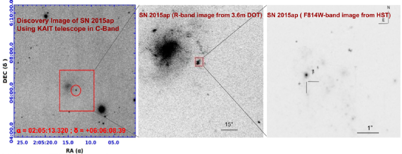
Figure 1: Left panel: The discovery image of SN 2015ap using the KAIT telescope in C-filter.The SN is marked inside the red circle. . Middle panel: A zoomed version of an $R$-band image with $2^{\prime}\times 2^{\prime}$ FoV obtained on 6 Oct. 2020 using a 4k $\times$ 4k CCD imager mounted on the 3.6 m DOT. Right panel: A further zoomed, about $6^{\prime\prime}\times 6^{\prime\prime}$ FoV of the location of SN 2015ap taken on 12 Aug. 2020 using the Hubble Space Telescope (HST) in the F814W filter. The SN seems to be fainter than the detection limit of HST at this time. A log of HST observations is included in the Appendix.

2 Data acquisition and reduction

SN 2015ap was discovered by KAIT as part of the Lick Observatory Supernova Search (LOSS; Filippenko et al., 2001), in an 18 s unfiltered image (close to the $R$ band; see Li et al. 2003) taken at 11:16:31 on 2015 Sep. 08 (Ross et al., 2015), at $17.41\pm 0.06$ mag. The object was also marginally detected one day earlier on Sep. 07.47 with $18.07\pm 0.22$  mag. We measure its J2000.0 coordinates to be $\alpha=02^{\mathrm{h}}05^{\mathrm{m}}13.32^{\mathrm{s}}$, $\delta=+06^{\circ}06\arcmin 08\aas@@fstack{\prime\prime}4$, with an uncertainty of $0\aas@@fstack{\prime\prime}5$ in each coordinate. SN 2015ap is $28\aas@@fstack{\prime\prime}3$ west and $16\aas@@fstack{\prime\prime}2$ south of the nucleus of its host galaxy IC 1776, which has a redshift of $z=0.011375\pm 0.000017$ (Chengalur et al., 1993) and a barred-spiral morphology (SB(s)d; de Vaucouleurs et al., 1991)). SN 2016bau was discovered by Ron Arbour in an unfiltered image taken at 23:22:33 on 2016 Mar. 13 (Arbour, 2016), at 17.8 mag. Its J2000.0 coordinates are given as $\alpha=11^{\mathrm{h}}20^{\mathrm{m}}59.02{\mathrm{s}}$, $\delta=+53^{\circ}10\arcmin 25\aas@@fstack{\prime\prime}6$. SN 2016bau is $35\aas@@fstack{\prime\prime}3$ west and $15\aas@@fstack{\prime\prime}2$ north of the nucleus of its host galaxy NGC 3631, which has $z=0.00384\pm 0.00014$ (Falco et al., 1999) and a morphology of SAc C (Ann, Seo & Ha, 2015). Both of these SNe were classified as SN Ib on the basis of well-developed features of He I, Fe II (blended), and Ca II, a few days after maximum brightness.

Figure 1 shows finder charts of SN 2015ap obtained with different telescopes. The $B$, $V$, $R$, and $I$ follow-up images of SN 2015ap and SN 2016bau were obtained with both the 0.76 m Katzman Automatic Imaging Telescope (KAIT; Filippenko et al., 2001) and the 1 m Nickel telescope at Lick Observatory. All images were reduced using a custom pipeline detailed by Stahl et al. (2019). Here, we briefly summarise the process for photometry. The image-subtraction procedures were applied in order to remove the host-galaxy light, using additional images obtained after the SN had faded below our detection limit. Point-spread-function (PSF) photometry was obtained using DAOPHOT (Stetson, 1987) from the IDL Astronomy User's Library. Three nearby stars were chosen from the Pan-STARRS1 catalogue for calibration. Their magnitudes were first transformed into Landolt (1992) magnitudes using the empirical prescription presented by Torny et al. (2012, Eq. 6) and then transformed to the KAIT/Nickel natural system. Apparent magnitudes were all measured in the KAIT4/Nickel2 natural system. The final results were transformed to the standard system using local calibrators and colour terms for KAIT4 and Nickel2 (Stahl et al., 2019). In addition, the $U$-band photometry was obtained from the Swift Optical/Ultraviolet Supernova Archive (SOUSA; https://archive.stsci.edu/prepds/sousa/; Brown et al. 2014).

There are a total of 17 spectra of SN 2015ap; 15 of them were taken with the Kast spectrograph (Miler & Stone, 1993) on the 3 m Shane telescope at Lick Observatory and the other 2 were taken with LRIS (Oke et al., 1995) on the Keck-I 10 m telescope. Except for the earliest spectrum taken on 10.531 Sep. 2015 (UT dates are used throughout this paper) using the Lick Shane/Kast system, 16 spectra in this paper were published by Shivvers et al. (2018); refer to that paper for details of the observations. Also, there are 8 spectra of SN 2016bau, all obtained with the Lick Shane/Kast system. We used the 600/4310 grism on the blue side, the 300/7500 grating on the red side, the d5500 dichroic, and a long slit $2^{\prime\prime}$ wide. For LRIS we used the 600/4000 grism on the blue side, the 400/8500 grating on the red side, and a $1^{\prime\prime}$ slit. The spectra were binned to 2 $\mathrm{\SIUnitSymbolAngstrom}$ pixel^-1.

3 Photometric Properties

In this section, we discuss various photometric properties of SN 2015ap and SN 2016bau, including their colour evolution, extinction, quasi-bolometric light curves, and various blackbody parameters.

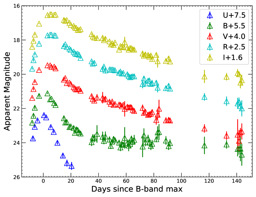
Figure 2: $UBVRI$ light curves of SN 2015ap, where $BVRI$ data were obtained with KAIT while the $U$-band data were taken from the UVOT mounted on Swift (https://swift.gsfc.nasa.gov).

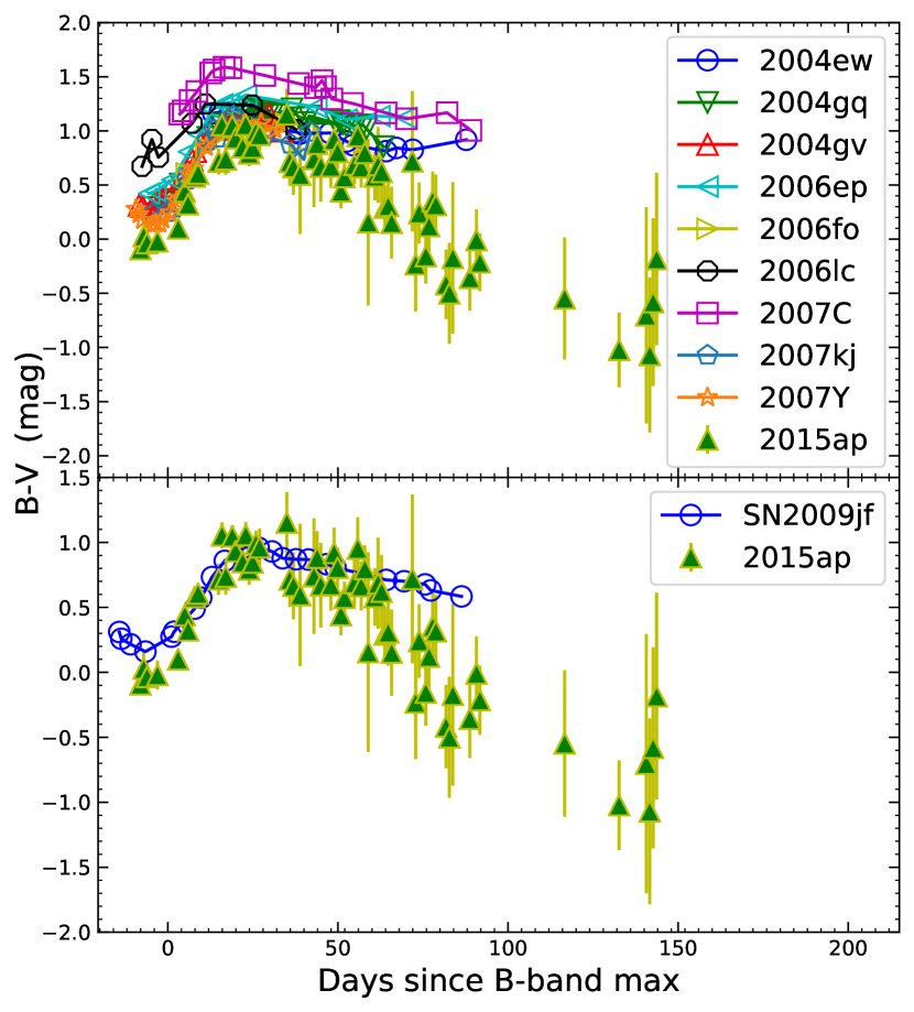
Figure 3: The top panel shows a comparison of the $(B-V)$ colour of SN 2015ap (corrected for Milky Way extinction) with that of other Type Ib SNe. The data for SNe other than SN 2015ap are taken from Stritzinger et al. (2018). The bottom panel shows the $(B-V)$ colour curves of SN 2015ap and SN 2009jf (both corrected for Milky Way extinction).

3.1 Photometric properties of SN2015ap

Most of the analysis in this paper has been performed with respect to $B$-band maximum brightness. To find its date, we fit a sixth-order polynomial to the $B$ data which well sample the photospheric phase. The resulting date of $B$-band maximum is MJD $57282.47\pm 2.56$. To determine the explosion epoch ($t_{\rm exp}$) of SN 2015ap, we use $R$-band data. The $R$ magnitudes are converted into fluxes and a sixth-order polynomial is fitted. We extrapolate the polynomial and the epoch corresponding to zero flux is taken as the explosion epoch, MJD $57272.72\pm 1.49$, which is in good agreement with Prentice et al. (2019).

Figure 2 shows the $UBVRI$ light curves of SN 2015ap. The rise rate for the $U$-band light curve is faster than that of other bands, and similarly the $U$ decline rate is faster, making the $U$ light curve much narrower compared to other bands. As we go to longer wavelengths, we see that the light curves become broader, with the $I$-band light curve being the broadest.

3.1.1 Colour evolution and extinction correction

Distances are taken from the NASA Extragalctic Database (NED), and a cosmological model with H${}_{0}=73.8$ km s^-1 Mpc^-1, $\Omega_{m}=0.3$, and $\Omega_{\Lambda}=0.7$ is assumed throughout. For SN 2015ap, we corrected for Milky Way (MW) extinction using NED following Schlafly & Finkbeiner (2011). In the direction of SN 2015ap, the Galactic extinctions for the $U$, $B$, $V$, $R$, and $I$ bands are 0.185, 0.154, 0.117, 0.092, and 0.064 mag, respectively.

The top panel of Figure 3 shows a comparison of the $(B-V)$ colour of SN 2015ap with that of other Type Ib SNe (all corrected for MW extinction). SN 2015ap seems to be the least reddened and lies below nearly all of the other SNe Ib.

Following Prentice et al. (2019), the host-galaxy contamination is negligible and hence ignored. To further support this assumption, the $(B-V)$ colour curve of SN 2009jf (Sahu et al., 2011) is shown in the bottom panel of Figure 3, corrected for an MW colour excess of $E(B-V)_{\rm MW}=0.112$ mag (host extinction is negligible). In order to match the ($B-V$) colour curve of SN 2009jf, we need not apply any shift to the MW-corrected SN 2015ap $(B-V)$ colour curve.

Figure 4 illustrates the position of SN 2015ap in the Miller diagram (Richardson et al., 2014). The distance modulus ($\mu$) of SN 2015ap is 33.269 mag; thus, SN 2015ap appears to be a normal SN Ib. For SN 2016bau, we calculate $\mu=32.65$ mag; based on its position in Figure 4, it seems to be a moderately luminous, normal SN Ib.

3.1.2 Quasi-bolometric and bolometric light curves

To obtain the quasi-bolometric light curves, we made use of the superbol code (Nicholl M., 2018). We first provided the extinction-corrected $U$, $B$, $V$, $R$, and $I$ data to superbol. Thereafter, it mapped the light curve in each filter to a common set of times through the processes of interpolation and extrapolation. It then fit blackbodies to the spectral energy distribution (SED) at each epoch, up to the observed wavelength, to give the quasi-bolometric light curve by performing trapezoidal integration. The peak quasi-bolometric luminosity obtained through integrating the flux over a wavelength range of 4000–10,000 $\mathrm{\SIUnitSymbolAngstrom}$ is $10^{(42.548\pm 0.019)}$ erg s^-1, in agreement with Prentice et al. (2019).

Figure 5 shows a comparison of the quasi-bolometric light curve of SN 2015ap with that of other H-stripped CCSNe. The code superbol also provides the bolometric light curve, including the additional blackbody corrections to the observed quasi-bolometric light curve, by fitting a single blackbody to observed fluxes at a particular epoch and integrating the fluxes trapezoidally for a wavelength range of 100–25,000 $\mathrm{\SIUnitSymbolAngstrom}$. The top panel of Figure 6 provides the resulting quasi-bolometric and bolometric light curves of SN 2015ap.

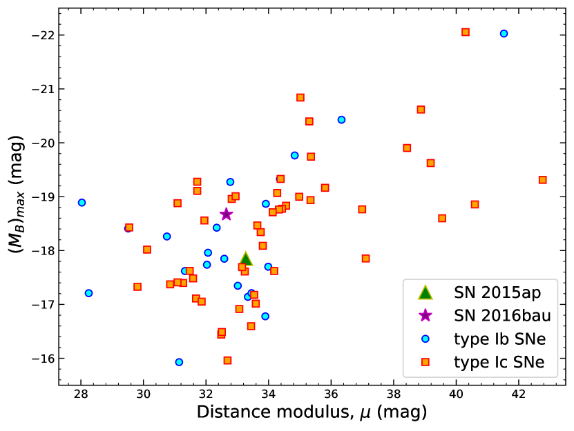
Figure 4: The position of SN 2015ap and SN 2016bau in the Miller diagram.

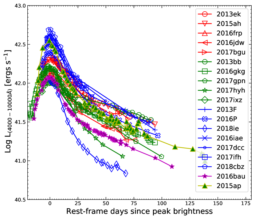
Figure 5: Comparison of quasi-bolometric light curves of SN 2015ap and SN 2016bau, obtained by fitting a blackbody to the SED and integrating the fluxes over the wavelength range of 4000–10,000 $\mathrm{\SIUnitSymbolAngstrom}$, with that of other stripped-envelope CCSNe. Symbols are colour coded: red, green, and blue correspond to Type Ib, IIb, and Ic SNe, respectively.

3.1.3 Temperature, radius, and velocity evolution

From superbol, the photospheric temperature ($T_{\rm BB}$) and radius ($R_{\rm BB}$) evolution of SN 2015ap are also obtained. During the initial phases, the photospheric temperature is high, reaching about 11,400 K at $-6.18$ d. Further, as the SN ejecta expand, cooling occurs and the temperature tends to fall, dropping to 4490 K on +21.66 d, then remaining nearly constant (Fig. 6, second panel from top). A conventional evolution in radius is also seen. Initially, at an epoch of $-8$ d, the photospheric radius is $4.14\times 10^{14}$ cm. Thereafter, the SN expands and its radius increases, reaching a maximum radius of $3.27\times 10^{15}$ cm, beyond which the photosphere seems to recede into the SN ejecta (Fig. 6, third panel from top). From the prior knowledge of the explosion epoch and radii at various epochs, we can estimate the photospheric velocity evolution of this SN, using $v_{\rm ph}=R_{\rm BB}/t$, where $t$ is the time since explosion. The bottom panel of Figure 6 shows the velocity evolution of SN 2015ap.

From the known value of $t_{\rm exp}$, a rise time ($t_{\rm rise}$) of $14.8\pm 2.2$ d is obtained. The photospheric velocity near maximum light is 9000 km s^-1 (Prentice et al., 2019). With the known values of $t_{\rm rise}$, the photospheric velocity near maximum light, and a constant opacity ($\kappa$) of 0.07 cm² g^-1, we also obtain the ejecta mass ($M_{\rm ej}$) and kinetic energy ($E_{\rm ke}$) from the Arnett (1982) model by following Equations (1) and (3) of Wheeler et al. (2015): $2.2\pm 0.6\,M_{\odot}$ and $(1.05\pm 0.31)\times 10^{51}$ erg, respectively. Our derived ejecta mass is slightly higher than that of Prentice et al. (2019), but less than Gangopadhyay et al. (2020). Corresponding to a peak luminosity of $(3.53\pm 0.16)\times 10^{42}$ erg s^-1, the amount of ⁵⁶Ni synthesised is $0.14\pm 0.02\,M_{\odot}$, calculated following Prentice et al. (2016).

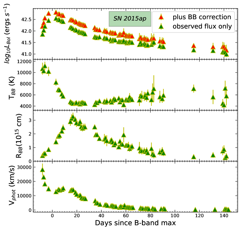
Figure 6: The top panel shows the bolometric and quasi-bolometric light curves of SN 2015ap. Second panel: the temperature evolution of SN 2015ap. Third and fourth panels: the radius and velocity evolutions (respectively) obtained using blackbody fits.

3.2 Photometric properties of SN 2016bau

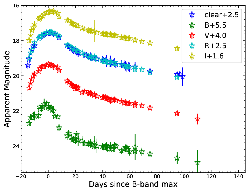
Figure 7: $BVRI$ and Clear filter light curves of SN 2016bau.

Following a method similar to that for SN 2015ap, the $B$-band maximum and the explosion epochs of SN 2016bau were determined to be MJD $57477.37\pm 1.99$ and MJD $57462.54\pm 0.97$, respectively. Figure 7 shows the $BVRI$ and Clear ($C$) filter light curves of SN 2016bau. Light curves in the shorter-wavelength bands are narrower compared to those in the longer-wavelength bands, following a trend similar to that of SN 2015ap. Also, the $C$ filter almost exactly replicates the $R$-band light curve, as expected (Li et al., 2003).

3.2.1 Colour evolution and extinction correction

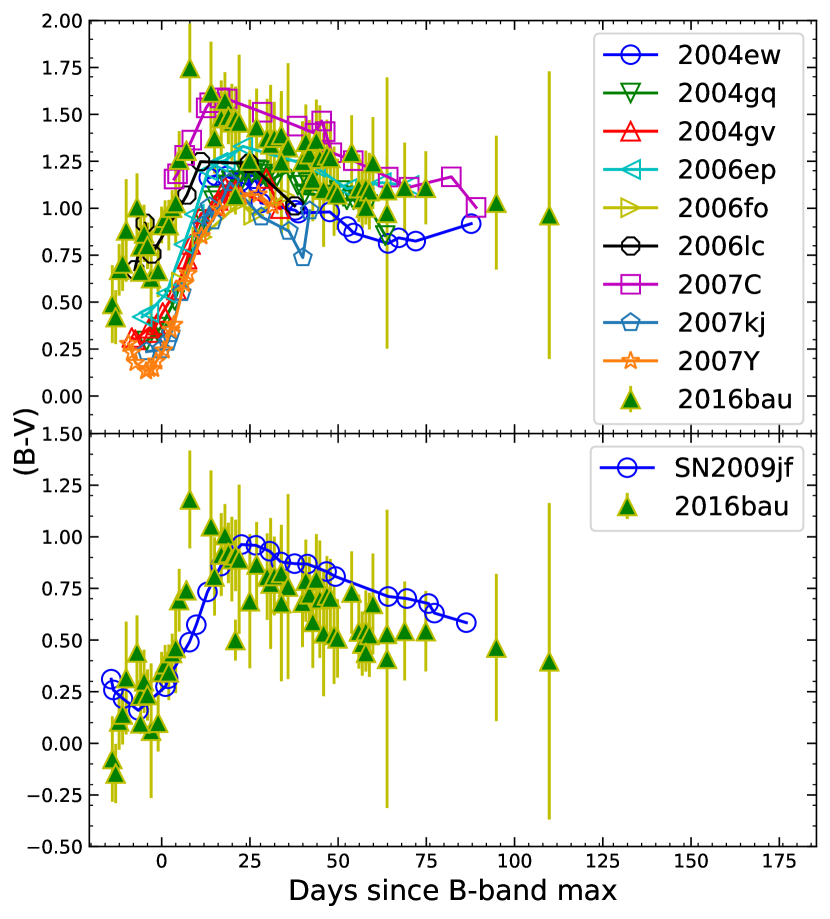
Figure 8: The top panel shows a comparison of the $(B-V)$ colour of SN 2016bau with that of other SNe Ib (all corrected for MW extinction). The data for the other SNe are taken from Stritzinger et al. (2018). The bottom panel shows the $(B-V)$ colour curves of SN 2016bau and SN 2009jf, both corrected for MW extinction. To match the SN 2009jf colour curve, a shift of 0.566 mag is required for the SN 2016bau colour curve.

Similar to SN 2015ap, we corrected for MW extinction using NED following Schlafly & Finkbeiner (2011). In the direction of SN 2016bau, the Galactic extinction for the $B$, $V$, $R$, and $I$ bands is 0.060, 0.045, 0.036, and 0.025 mag, respectively. The top panel of Figure 8 shows a comparison of the $(B-V)$ colour of SN 2016bau with that of other SNe Ib. SN 2016bau seems to be heavily reddened and lies above nearly all of the other SNe Ib. To correct for the host-galaxy extinction, we made use of the colour curve of SN 2009jf. We calculated the differences in the colours of the two SNe and took their weighted mean. In this calculation, we made use of data only in the range 0 to +20 d for the reasons mentioned by Stritzinger et al. (2018). The resulting host-galaxy extinction is $E(B-V)_{\rm host}=0.566\pm 0.046$ mag. Thus, in order to match the SN 2009jf $(B-V)$ colour curve, we need to shift the MW-corrected $(B-V)$ colour curve of SN 2016bau downward by 0.566 mag, as shown in the bottom panel of Figure 8.

3.2.2 Quasi-bolometric and bolometric light curves

To obtain the quasi-bolometric and bolometric light curves of SN 2016bau, we used superbol, as in the case of SN 2015ap. The extinction-corrected $B$, $V$, $R$, and $I$ data were given as input to superbol. The top panel of Figure 9 shows the quasi-bolometric and bolometric light curves of SN 2016bau. Figure 5 shows the comparison of the quasi-bolometric light curve of SN 2016bau obtained by integrating the flux over the wavelength range 4000–10,000 Å with other H-stripped CCSNe from Prentice et al. (2019). Here, SN 2016bau also seems to lie on the moderately bright end.

3.2.3 Temperature, radius, and velocity evolution

Figure 9 also shows the evolution of the photospheric temperature ($T_{\rm BB}$) and radius ($R_{\rm BB}$) of SN 2016bau, obtained using superbol. During the initial phases, the photospheric temperature is very high, reaching about 17,000 K near 0 d. Thereafter, as the SN ejecta expand, cooling occurs and the temperature falls, reaching 6000 K at around +20 d, then remaining nearly constant (Fig. 9, second panel from top). A conventional evolution in radius is also seen (Fig. 9, third panel from top). Initially, at an epoch of around $-6$ d, the photospheric radius is $0.28\times 10^{15}$ cm. Following this, the supernova expands and its radius increases, reaching a maximum radius of $0.96\times 10^{15}$ cm, beyond which the photosphere seems to recede within the SN ejecta.

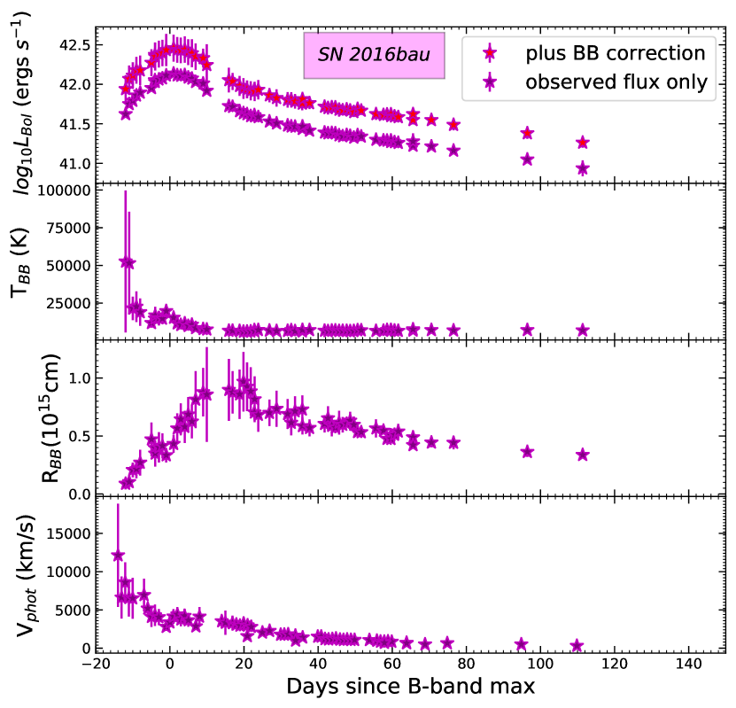
Figure 9: The top panel shows the bolometric and quasi-bolometric light curves of SN 2016bau. Second panel: the temperature evolution of SN 2016bau. Third and fourth panels: the radius and velocity evolution (respectively) obtained using blackbody fits.

From the prior knowledge of explosion epoch and radii at various epochs, we estimate the photospheric velocity evolution of this SN in the same way as for SN 2015ap. The bottom panel of Figure 9 shows the velocity evolution of SN 2016bau.

From the prior knowledge of $t_{\rm exp}$, a rise time ($t_{\rm rise}$) of $17.09\pm 1.29$ d is obtained. The photospheric velocity near maximum light is $\sim 5000$ km s^-1, obtained from a blackbody fit. With the known values of $t_{\rm rise}$, the photospheric velocity near maximum light, and a constant opacity ($\kappa$) 0.07 cm² g^-1, we obtain the ejecta mass ($M_{\rm ej}$) and kinetic energy ($E_{\rm ke}$) following Equation (1) and Equation (3) of Wheeler et al. (2015); the results are $1.6\pm 0.3\,M_{\odot}$ and $(0.24\pm 0.04)\times 10^{51}$ erg, respectively. Following Prentice et al. (2016), an amount of $0.055\pm 0.006\,M_{\odot}$ of ⁵⁶Ni is synthesised, corresponding to a peak luminosity of $(1.19\pm 0.08)\times 10^{42}$ erg s^-1.

4 Spectral studies of SN 2015ap and SN 2016bau

In this section, we discuss spectral features of SN 2015ap and SN 2016bau and further compare their properties with other similar SNe. We modelled the spectra of these two SNe at different epochs using SYN++ (Branch et al., 2007; Thomas et al., 2011) and performed the spectral matching of the 12, 13, and 17 $M_{\odot}$ spectral models given by Jerkstrand (2015) with the spectra of SN 2015ap and SN 2016bau at phases around 100 d past explosion. In this section, we also estimate the velocities of various lines present in the spectra, using their absorption troughs.

4.1 Spectral properties of SN 2015ap

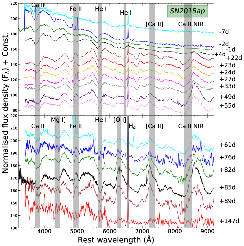
Figure 10: Top panel: the early-phase spectra up to +55 d. Bottom panel: the spectral evolution beyond +55 d since $B_{\rm max}$ of SN 2015ap.

The top and bottom panels of Figure 10 show the early phases ($-7$ d to +55 d) and late phases (+61 d to +147 d) spectral evolution, respectively. It is quite evident from the top panel of Figure 10 that initially SN 2015ap shows broad-lined features (at $-7$ d and $-2$ d), which later evolve to spectra of a normal Type Ib SN. The characteristic He I line at 5876 $\mathrm{\SIUnitSymbolAngstrom}$ of a typical SN Ib is clearly seen in the spectra of SN 2015ap. We also see unambiguous He I features at 6678 $\mathrm{\SIUnitSymbolAngstrom}$ and 7065 $\mathrm{\SIUnitSymbolAngstrom}$, but these two lines are not as prominent as the one at 5876 $\mathrm{\SIUnitSymbolAngstrom}$. In the very early phases (up to +4 d), the He I line at 7065 $\mathrm{\SIUnitSymbolAngstrom}$ is hard to identify. We see that the He I absorption at 5876 $\mathrm{\SIUnitSymbolAngstrom}$ is stronger than any other absorption features, and it is present in every spectrum up to +147 d. The Fe II feature near 5169 $\mathrm{\SIUnitSymbolAngstrom}$ is very hard to be identified, and it seems to be highly blended with He I 5016 $\mathrm{\SIUnitSymbolAngstrom}$.

The spectral evolution also shows the Ca II near-infrared (NIR) feature, which is almost absent in the very early phases ($-7$ d to +4 d), but starts to develop very strongly from +22 d onward. It is so strong that each spectrum on and after +22 d shows it, even the lowest-SNR spectrum at +147 d. The forbidden [Ca II] feature near 7300 $\mathrm{\SIUnitSymbolAngstrom}$ is almost absent at very early phases ($-7$ d to +4 d), then begins to develop very obviously in the spectra from +22 d, and is present up to +89 d. This [Ca II] feature can also get blended with [O II] emission at 7320 $\mathrm{\SIUnitSymbolAngstrom}$ and 7330 $\mathrm{\SIUnitSymbolAngstrom}$. It almost disappears in the spectrum at +147 d, though its absence may not be real owing to the very poor SNR of that spectrum. We also see the Ca II H&K feature near 3934 $\mathrm{\SIUnitSymbolAngstrom}$, which is present in every spectrum. From the bottom panel of Figure 10, we see that as the spectra evolve, the absorption features of different lines tend to disappear and the emission features become more prominent. We see a very weak semiforbidden Mg I] line, at 4571 $\mathrm{\SIUnitSymbolAngstrom}$. However we can clearly see the forbidden emission lines of [O I] and [Ca II], which indicates the onset of the nebular phase.

4.1.1 Spectral comparison

To investigate the spectroscopic behaviour of SN 2015ap, we compare its spectral features with those of other well-studied SNe Ib such as SN 2004gq (Modjaz et al., 2014), SN 2008D (Modjaz et al., 2014), SN 2012au (Pandey et al., 2020), SN 2009jf (Sahu et al., 2011; Modjaz et al., 2014), iPTF13bvn (Srivastav et al., 2014a), SN 2007uy (Modjaz et al., 2014; Milisavljevic et al., 2010), SN 2007gr (Valenti et al., 2008; Modjaz et al., 2014), and SN 2005bf (Modjaz et al., 2014).

The top panel of Figure 11 shows the early phase ($-7$ d) spectral comparison of SN 2015ap with these well-studied SNe Ib. The spectral features of SN 2015ap look similar to those of SN 2008D and SN 2012au, compared to other SNe Ib. We can see that the Ca II H&K feature, the Mg II feature, and the He I P Cygni profile match very well with those of SN 2008D, while in other SNe in the comparison sample, these features are much more developed. The blue end of the spectrum matches nicely with SN 2008D, while the redder part is featureless and much closer to SN 2012au and SN 2005bf. The He I 5876 $\mathrm{\SIUnitSymbolAngstrom}$ feature of SN 2015ap is completely different from that of SN 2007uy, but resembles that of SN 2008D and seems to be less evolved compared to that of SN 2004gq, SN 2012au, SN 2009jf, and iptf13bvn. The Fe II profile in SN 2015ap is hard to detect, which may be due to a very high initial optical opacity. We try to estimate the velocities using the various absorption features. As the spectrum at this epoch is continuum dominated, only a few absorption features were visible. The velocity estimated using He I absorption lines is $\sim$ 14,100 km s^-1.

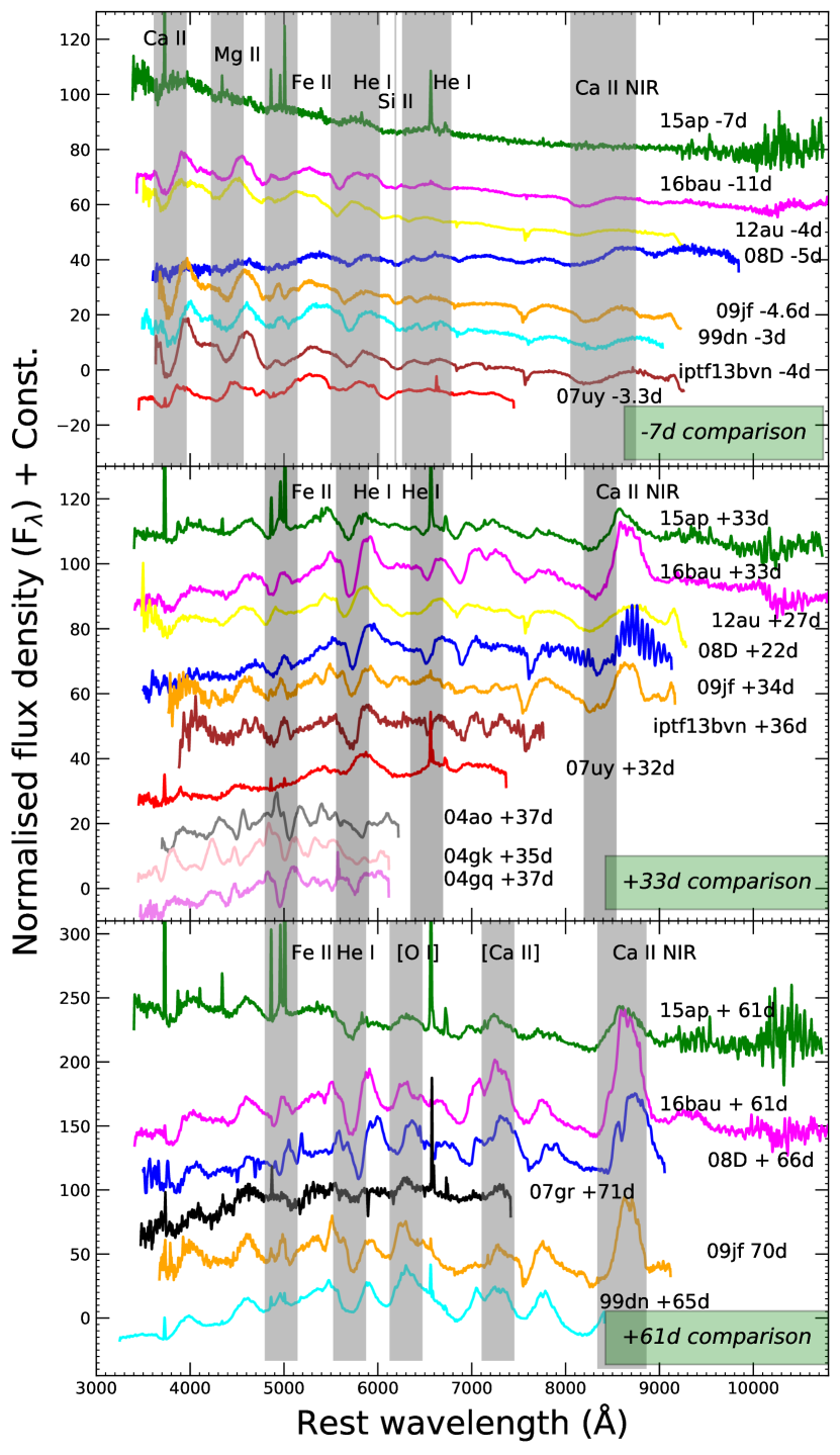
Figure 11: Spectral comparison of the spectra of SN 2015ap and SN 2016bau at epochs $-7$ d (top panel), +33 d (middle panel), and +61 d (bottom panel). Various important SN Ib features have been compared with those of other similar-type SNe.

Further, we compare the +33 d spectrum of SN 2015ap with our comparison sample (middle panel of Figure 11). At this epoch, the spectrum of SN 2015ap shows various P Cygni profiles. We see that it almost exactly replicates the +22 d spectrum of SN 2008D. The blended He I and Fe II profiles near 5016 $\mathrm{\SIUnitSymbolAngstrom}$ well match those of other SNe Ib, except for SN 2007uy, where the peak is almost absent, and for SN 2005bf, where it is double peaked. The He I feature at 5876 $\mathrm{\SIUnitSymbolAngstrom}$ matches well with other SNe Ib except for the cases of SN 2007uy and SN 2005bf, where the absorption features seem to be much broader. Here, once again, SN 2007uy seems to match much less and SN 2008D seems to best match the +22 d spectrum of SN 2015ap. The velocities estimated using the Ca II NIR triplet and He I absorption features are $\sim$ 7800 km s^-1 and 10000 km s^-1, respectively.

For a much clear comparison, we compared the +61 d spectrum of SN 2015ap (bottom panel of Fig. 11) with spectra of other well-studied SNe Ib. At this epoch also, the spectrum is still much closer to that of SN 2008D compared to other SNe Ib. The blended Fe II and He I feature near 5016 $\mathrm{\SIUnitSymbolAngstrom}$ shows an almost similar profile to that of SN 2008D. However, the 5876 $\mathrm{\SIUnitSymbolAngstrom}$ He I profile is narrower in SN 2015ap compared to SN 2008D. We can see the onset of the appearance of the [O I] line in SN 2015ap, which differs from SN 2008D. The He I profile is well matched in the cases of SN 1999dn and SN 2009jf, but the Ca II NIR triplet of these SNe differs from that of SN 2015ap. Here the velocities estimated using the Ca II NIR triplet and He I absorption features are $\sim$ 6900 km s^-1 and 8100  km s^-1, respectively.

4.1.2 Spectral modelling

After confidently identifying the features present in the spectra of SN 2015ap and comparing them with those of other well-studied SNe, we tried to model a few spectra at various epochs using SYN++. The top panel in Figure 12 shows the early-phase ($-7$ d) spectrum of SN 2015ap. This spectrum displays weak and broad P Cygni profiles of He I, Ca II H&K, and the Ca II NIR triplet, and also some blended features of Fe II. We also show the best-matching synthetic spectrum, generated by SYN++. The absorption features due to Ca II H&K, Ca II NIR triplet, He I, and Fe II multiplets are easily reproduced. The photospheric velocity and blackbody temperature associated with the best-fit spectrum are 12,000 km s^-1 and 12,000 K, respectively. We perform SYN++ matching to four additional spectra from epochs $-2$ d to +33 d (Fig. 12). With the passage of time, the SN expands, cools gradually, and its expansion velocity decreases slowly, so we see a gradual decrease in the values of these fitted parameters. The photospheric velocities during the phase of $-7$ d to +33 d vary from 13,000 km s^-1 to 6800 km s^-1, and the blackbody temperature varies from 12,000 K to 4500 K, which are in good agreement with those obtained photometrically from blackbody fits. Owing to the local thermodynamic equilibrium (LTE) approximation, SYN++ does not work well for the later epochs and cannot be used to fit the spectra.

To get an estimate of the progenitor mass, we used the +98.75 d post-explosion spectrum of SN 2015ap and plotted it along with the 12, 13, and 17 $M_{\odot}$ model spectra from Jerkstrand (2015) at 100 d, after scaling by a factor of exp$(-2\times\Delta t/111.4)$ (Jerkstrand, 2015), where $\Delta t$ = 1.25, is the time difference between the epoch of the model spectrum and the epoch of the observed spectrum. We can see that the 12 $M_{\odot}$ and 17 $M_{\odot}$ model spectra seem to reproduce the observed spectrum of SN 2015ap. The 12 $M_{\odot}$ spectrum very nicely matches the observed spectrum throughout the entire wavelength range, while the 17 $M_{\odot}$ spectrum slightly overproduces the flux near the Ca II NIR triplet close to 8500 $\mathrm{\SIUnitSymbolAngstrom}$. However, the 13 $M_{\odot}$ model spectrum fails to explain the observed fluxes throughout the entire wavelength range. Thus, based on this analysis, a range of 12–17 $M_{\odot}$ is expected for the possible progenitor mass of SN 2015ap, in agreement with that described by Gangopadhyay et al. (2020).

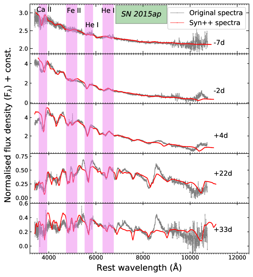
Figure 12: SYN++ modelling of the spectra of SN 2015ap at epochs $-7$ d, -2 d, +4 d, +22 d, and +33 d. Prominent He I features could be produced nicely.

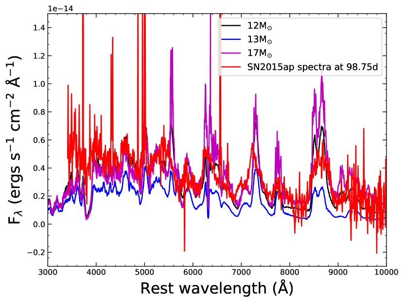
Figure 13: The $t=+98.75$ d spectrum of SN 2015ap plotted along with the 12, 13, and 17 $M_{\odot}$ models from Jerkstrand (2015) at 100 d scaled with an exponential factor exp$(-2\times 1.25/111.4)$. The 12 $M_{\odot}$ and 17 $M_{\odot}$ models seem to best match the observed spectrum of SN 2015ap.

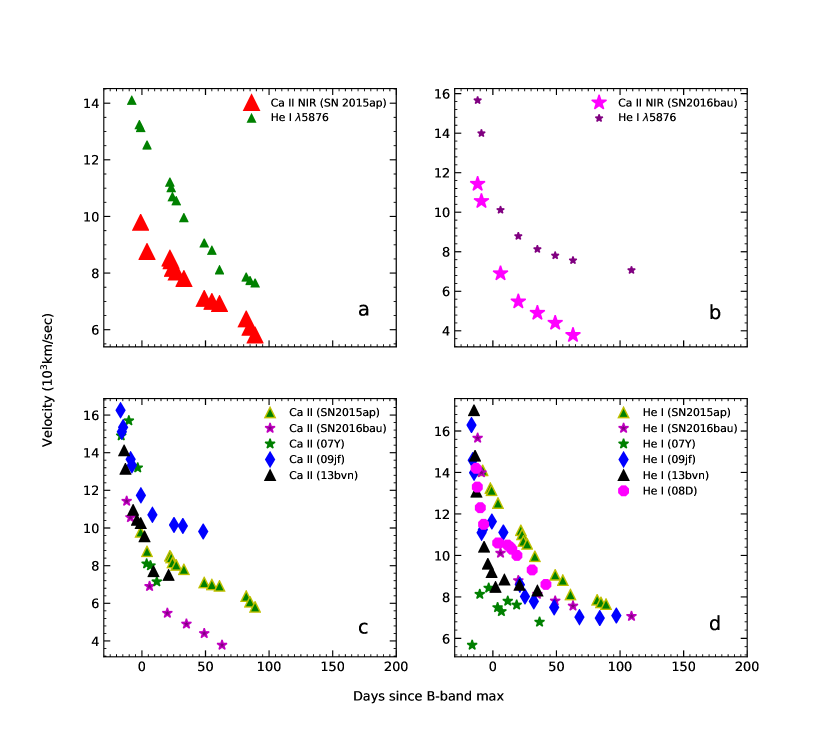
Figure 14: (a) The temporal evolution of velocities of He I 5876 $\mathrm{\SIUnitSymbolAngstrom}$ and the Ca II NIR triplet for SN 2015ap. (b) Same as (a) but for SN 2016bau. The bottom two panels show the comparison of these line velocities of SN 2015ap and SN 2016bau with SNe 2007Y (Stritzinger et al., 2009), 2009jf (Sahu et al., 2011), iPTF13bvn (Srivastav et al., 2014a), and 2008D (Modjaz et al., 2014).

4.1.3 Velocity evolution of various lines of SN 2015ap

We used the blue–shifted absorption minima of P Cygni profiles and the special-relativistic Doppler formula (Sher, 1968) to obtain the velocities of several lines. Figure 14$a$ shows the He I and the Ca II NIR triplet velocity evolution of SN 2015ap. In the initial few days, the line velocities tend to decrease rapidly. At an epoch of +24 d, the velocities estimated using He I 5876 $\mathrm{\SIUnitSymbolAngstrom}$ and the Ca II NIR triplet are $\sim$ 10,600 km s^-1 and 8200 km s^-1, respectively. The velocities estimated using these two lines drop to $\sim$ 9100 km s^-1 and 7100 km s^-1 (respectively) at an epoch of +49 d. In the late phases, the velocities decline gradually.

Figure 14$c,d$, show comparisons of velocities obtained using the Ca II NIR triplet and He I 5876 $\mathrm{\SIUnitSymbolAngstrom}$ features with other well-studied SNe. Initially the Ca II NIR line velocity of SN 2015ap evolves in a manner similar to iptf13bvn, thereafter it decays slowly, attaining a velocity of $\sim$ 7600 km s^-1 at +89 d. We see that the ejecta velocity of SN 2015ap obtained using He I 5876 $\mathrm{\SIUnitSymbolAngstrom}$ is higher than that of other SNe Ib but closer to SN 2008D.

4.2 Spectral properties of SN 2016bau

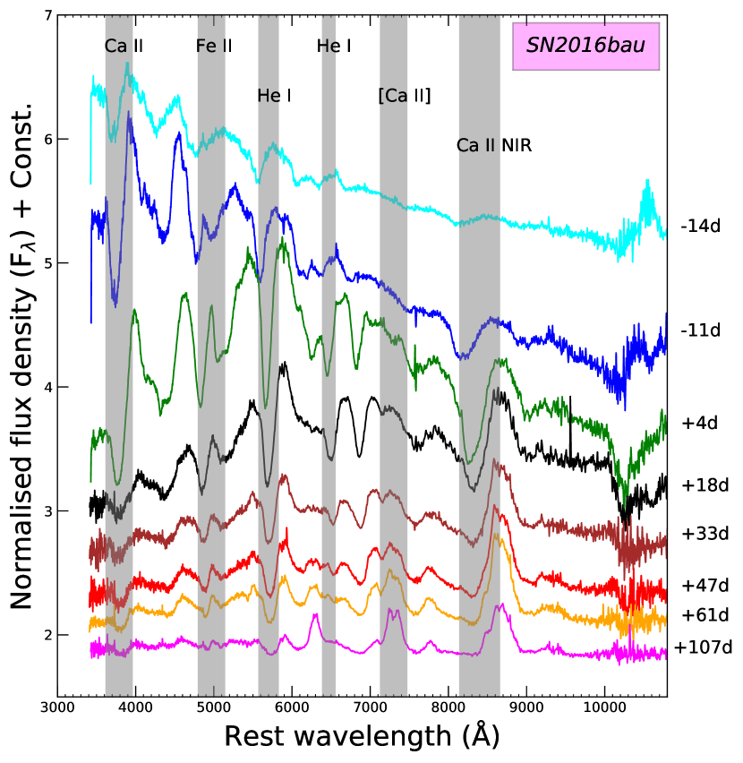
Figure 15: Various line identifications in the overall spectral evolution of SN 2016bau. Strong He I features along with other important lines are indicated.

Figure 15 shows the spectral evolution of SN 2016bau for a period of $-14$ d to +107 d. In the first spectrum ($-14$ d), we see well-developed He I features (5876, 6678, and 7065 $\mathrm{\SIUnitSymbolAngstrom}$). Also, the spectrum on this particular epoch displays a weak and broad Ca II NIR feature, but with the passage of time (beyond $\sim+33$ d), prominent Ca II NIR features start to appear. We also see that in the initial phases there is a strong Ca II H $\&$ K feature, but it becomes progressively weaker at later phases. As the phase approaches the date of $B$-band maximum brightness, the He I features start to appear much more strongly, as seen in the spectra at $-11$ d, +4 d, and +18 d. Beyond $-11$ d, the longer wavelengths exhibit strong Ca II NIR features. The spectra also display very strong P Cygni profiles of He I at 5016 $\mathrm{\SIUnitSymbolAngstrom}$ after $t=-11$ d. The emergence of very strong features of He I in the early-time spectra confirms this SN to be of Type Ib.

4.2.1 Spectral comparison

To investigate the spectroscopic behaviour of SN 2016bau, we have compared its spectral features with those of other well-studied SNe Ib. We used a sample similar to that for SN 2015ap. The top panel of Figure 11 shows the early-phase ($-11$ d) spectral comparison of SN 2016bau with other well-studied H-stripped CCSNe. The spectral features of SN 2016bau look much more similar to those of SN 2012au, SN 2009jf, and SN 1999dn compared to other SNe. we can see that the Ca II  H&K feature, the Mg II feature, and the He I P Cygni profile of SN 2016bau match very well those of SN 2012au, SN 2009jf, and SN 1999dn. The He I 5876 $\mathrm{\SIUnitSymbolAngstrom}$ feature of SN 2016bau is completely different from that of SN 2007uy, SN 2015ap, and SN2008D. As with SN 2015ap, the blended Fe II profile in SN 2016bau is hard to detect, which may be due to a very high initial optical opacity. The spectrum at this epoch has nicely developed He I features. The velocity estimated using the He I 5876 $\mathrm{\SIUnitSymbolAngstrom}$ absorption line is $\sim$ 15,600 km s^-1.

The middle panel of Figure 11 shows the +33 d spectral comparison of SN 2016bau with other well-studied SNe Ib. The spectrum at this epoch contains many P Cygni profiles of various lines. These spectral features look most similar to those of SN 2008D and SN 2015ap, compared to other SNe Ib. We see that the Ca II NIR feature, the Fe II feature, and the He I P Cygni profile match very well those of SN 2008D and SN 2015ap, compared to other SNe. SN 2009jf also seems to match nicely in the redder part of the spectrum. The He I 5876 $\mathrm{\SIUnitSymbolAngstrom}$ feature of SN 2016bau is completely different from those of SN 2007uy, SN 2005bf, SN 2004gq, and SN 2007gr, but resembles those of SN 2008D, SN 2015ap, and SN2009jf. The He I 5876 $\mathrm{\SIUnitSymbolAngstrom}$ profile of SN 2016bau seems to be more asymmetric and narrower than that of iptf13bvn. At this epoch, the velocities estimated using the absorption features of He I and the Ca II NIR triplet are $\sim$ 8100 km s^-1 and 4900 km s^-1, respectively.

For much clearer comparisons, we also compared the +61 d spectrum of SN 2016bau (bottom panel of Figure. 11) with other well-studied H-stripped CCSNe spectra. At this epoch, the bluer part of the spectrum is much closer to SN 2008D compared to other SNe Ib. Here the blended Fe II and He I features near 5016 $\mathrm{\SIUnitSymbolAngstrom}$ show profiles nearly similar to those of SN 2008D and SN 2009jf. However, the 5876 $\mathrm{\SIUnitSymbolAngstrom}$ He I profile is broader in SN 2016bau compared with SN 2008D. We can see that the onset of the appearance of [O I] in SN 2016bau is slightly different from that of SN 2008D, while it matches nicely that of SN 2009jf. The He I profile is well matched in the case of SN 2008D. Here the velocities estimated using the Ca II NIR and He I absorption features are $\sim$ 3700 km s^-1 and 7600 km s^-1, respectively.

4.2.2 Spectral modelling

After confidently identifying various spectral features, we tried to model the spectra of SN 2016bau at different epochs using SYN++. The top panel of Figure 16 shows the early-phase ($-14$ d) spectrum of SN 2016bau. It contains many broad P Cygni profiles of He I, Ca II H&K, the Ca II NIR triplet, and also some blended features of Fe II. In this figure we have also presented the best-matching synthetic spectrum generated by SYN++. The modelled spectrum easily reproduces the absorption features of Ca II H&K, Ca II NIR, He I, and the Fe II multiplet. The photospheric velocity and blackbody temperature associated with the best-fit spectrum are 16,000 km s^-1 and 9000 K respectively. We performed SYN++ matching for four additional spectra which covers a period of $-11$ d to +33 d (subsequent panels of Fig. 16). With the passage of time, the SN expands and cools gradually, and its expansion velocity decreases slowly, so we see a gradual decrease in the fit parameters such as velocity and temperature in the later phases. The photospheric velocity during the phase of $-14$ d to +33 d varies from 16,000 km s^-1 to 8000 km s^-1 and the blackbody temperature ranges from 9000 K to 4000 K, in good agreement with values obtained photometrically from blackbody fits.

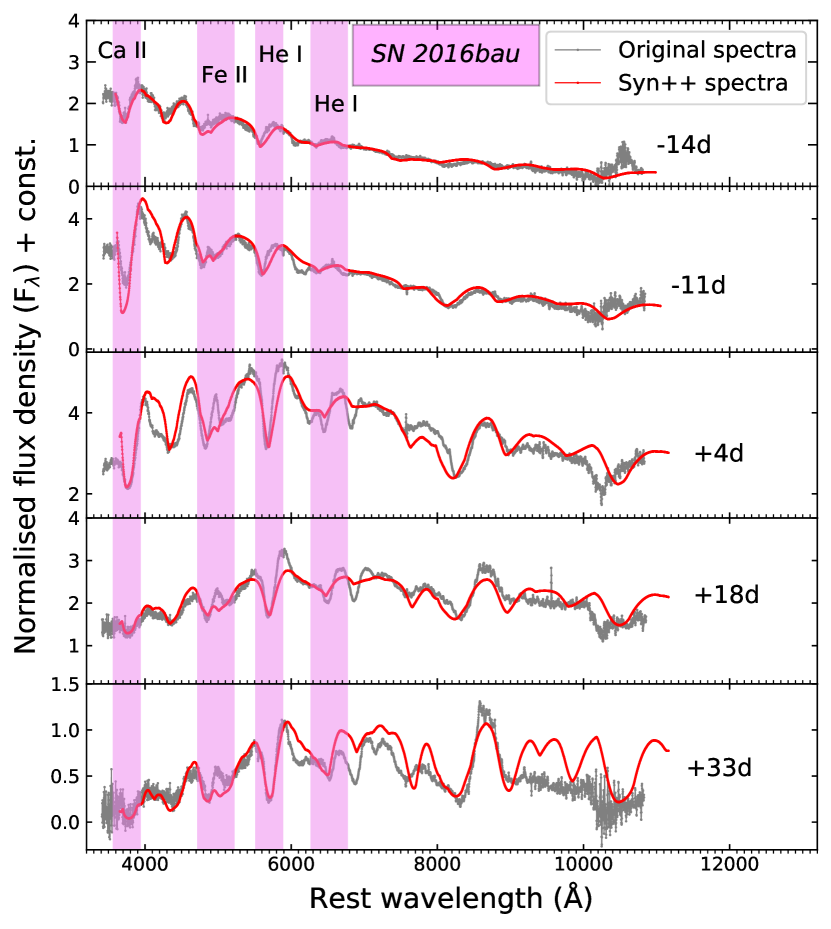
Figure 16: SYN++ modelling of the spectra of SN 2016bau at epochs $-14$ d, $-11$ d, $+4$ d, $+18$ d, and $+33$ d.

We also try to match the +121 d spectrum of SN 2016bau with the 12 $M_{\odot}$, 13 $M_{\odot}$, and 17 $M_{\odot}$ model spectra at +100 d from Jerkstrand (2015), scaled with a factor of exp$(-2\times\Delta t/111.4)$ (Jerkstrand, 2015), where $\Delta t$ = 21, is the time difference of the epoch of model spectrum and the epoch of observed spectrum. We can see that all three models over–predict the observed fluxes from 3000 $\mathrm{\SIUnitSymbolAngstrom}$ to around 6000 $\mathrm{\SIUnitSymbolAngstrom}$, beyond which the 12 $M_{\odot}$ model spectrum seems to best describe the observed spectrum. It could nicely explain the [Ca II] emission near 7300 $\mathrm{\SIUnitSymbolAngstrom}$ and the Ca II NIR feature near 8500 $\mathrm{\SIUnitSymbolAngstrom}$. The 13 $M_{\odot}$ model spectrum also produces the [Ca II] emission but fails to explain the observed fluxes near the Ca II-NIR triplet. The 17 $M_{\odot}$ model spectrum overpredicts the flux throughout the entire wavelength range and thus fails to explain the spectrum of SN 2016bau. Hence, based on our analysis, a slightly low-mass progenitor ($\leq 12$ $M_{\odot}$) is expected.

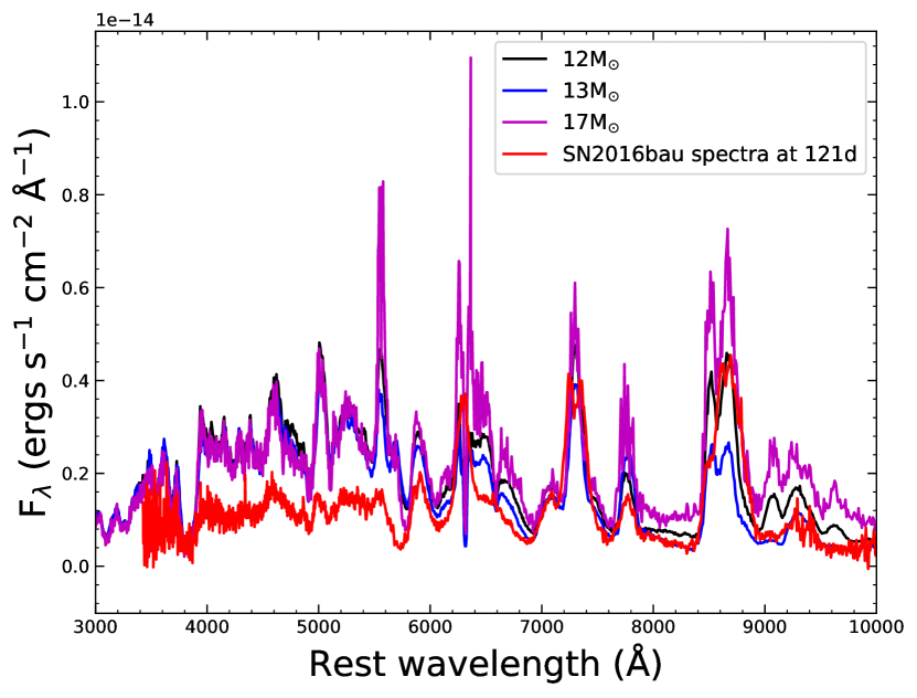
Figure 17: The $t=+121$ d spectrum of SN 2016bau plotted along with the 12, 13, and 17 $M_{\odot}$ models from Jerkstrand (2015) at 100 d scaled with an exponential factor exp$(-2\times 21/111.4)$. The 12 $M_{\odot}$ model seems to best match the spectrum of SN 2016bau.

4.2.3 Velocity evolution of Various lines of SN 2016bau

We used the blue-shifted absorption minima of P Cygni profiles to obtain the velocities of He I and Ca II NIR lines. Figure 14$b$ shows the He I and Ca II NIR velocity evolution of SN 2016bau. In the initial few days, the line velocities tend to decrease rapidly, but in later phases, the velocities decline gradually. At an early epoch of $-14$ d, the velocities estimated using He I 5876 $\mathrm{\SIUnitSymbolAngstrom}$ and the Ca II NIR triplet are $\sim$ 15,600 km s^-1 and $\sim$ 11,400 km s^-1, respectively. The velocities estimated using these two lines drop to $\sim$ 7800 km s^-1 and $\sim$ 4400 km s^-1 (respectively) at an epoch of +47 d. Beyond +47 d, the velocities continue to decline with a slower rate as compared to initial decline rate. Figure 14$c,d$ show the comparison of these two line velocities with other well-studied SNe. Initially, the Ca II NIR velocity declines very fast but in the later epochs, only gradual decline is seen. It evolves in a manner very similar to iPTF13bvn, but in the late phases, the velocities are slower than other SNe. The velocity obtained using He I 5876 $\mathrm{\SIUnitSymbolAngstrom}$ of SN 2016bau evolves in a manner similar to that of other SNe Ib, but much closer to SN 2009jf and iPTF13bvn. The He I line velocity of SN 2016bau at +33 d reaches $\sim$ 8200 km s^-1, nearly equal to those of SN 2009jf and iPTF13bvn.

5 MINIM modelling of the quasi-bolometric light curve

In this section, we fit the radioactive decay (RD) and the magnetar (MAG) powering mechanisms, as discussed by Chatzopoulous et al. 2013 (see also Wheeler et al. 2017; Kumar et al. 2020, 2021), by employing the MINIM (Chatzopoulous et al., 2013) code. MINIM is a $\chi^{2}$-minimisation fitting code that utilises the Price algorithm (Brachetti et al., 1997). In the RD model, the radioactive decay of ⁵⁶Ni and ⁵⁶Co leads to the deposition of energetic gamma-rays that are assumed to thermalise in the homologously expanding SN ejecta and thus powering the light curve. In the MAG model, the light curves are powered by the energy released by the spin-down of a young magnetar, located in the centre of the SN ejecta. Following Prentice et al. (2019), we have adopted a constant opacity, $\kappa$ = 0.07 cm² g^-1, for both SN 2015ap and SN 2016bau.

Table 1: Minimum $\chi^{2}$/dof parameters for SN 2015ap and SN 2016bau for the RD model.

	$M_{\mathrm{Ni}}$a	$t_{\mathrm{d}}$b	$A_{\mathrm{\gamma}}$c	$M_{\mathrm{ej}}$b	$\chi^{2}/\mathrm{dof}$
	($M_{\odot}$)	(days)		($M_{\odot}$)
SN 2015ap
whole light curve	0.094 $\pm$ 0.004	8.0 $\pm$ 2.0	30.05 $\pm$ 1.05	0.64 $\pm$ 0.3	6.2
+20 d data	0.181 $\pm$ 0.006	14.5 $\pm$ 0.3	5.3 $\pm$ 0.3	2.1 $\pm$ 0.09	1.2
SN 2016bau
whole light curve	0.08 $\pm$ 0.01	20.5 $\pm$ 0.7	7.8 $\pm$ 0.5	2.8 $\pm$ 0.2	22.7
+20 d data	0.065 $\pm$ 0.001	18.09 $\pm$ 0.3	9.95 $\pm$ 0.4	1.81 $\pm$ 0.07	1.2

$a$, mass of ⁵⁶Ni synthesised; $b$, effective diffusion timescale,
$c$, optical depth for the $\gamma$-rays measured 10 d after the explosion;
$d$, ejecta mass, with $\kappa=0.07$ cm² g^-1.

Table 2: Minimum $\chi^{2}$/dof parameters for SN 2015ap and SN 2016bau for the MAG model.

	$R_{0}$a	$E_{p}$b	$t_{d}$c	$t_{p}$d	$v_{\rm exp}$e	$M_{\rm ej}$f	$P_{i}$g	$B$h	$\chi^{2}/\mathrm{dof}$
	($10^{13}$ cm)	($10^{51}$ erg)	(days)	(days)	($10^{3}$ km s-1)	($M_{\odot}$)	(ms)	($10^{14}$ G)
SN 2015ap
	0.594 $\pm$ 0.003	0.01210 $\pm$ 0.00007	8.7 $\pm$ 0.1	12.06 $\pm$ 0.08	6.03 $\pm$ 0.02	0.75$\pm$ 0.02	40.6 $\pm$0.1	25.5$\pm$ 0.2	1.54
SN 2016bau
	7.9 $\pm$ 0.7	0.00403 $\pm$ 0.00007	8.5 $\pm$ 0.1	15.1 $\pm$ 0.1	6.2 $\pm$ 0.5	1.26$\pm$ 0.02	70.4$\pm$ 0.6	52.6$\pm$ 0.8	1.4

$a$, progenitor radius; $b$, magnetar rotational energy; $c$, effective diffusion timescale (in days); $d$, magnetar spin-down timescale;
$e$, SN expansion velocity; $f$, $\kappa=0.07$ cm² g^-1 is used; $g$, initial period of the magnetar; $h$, magnetic field of the magnetar.

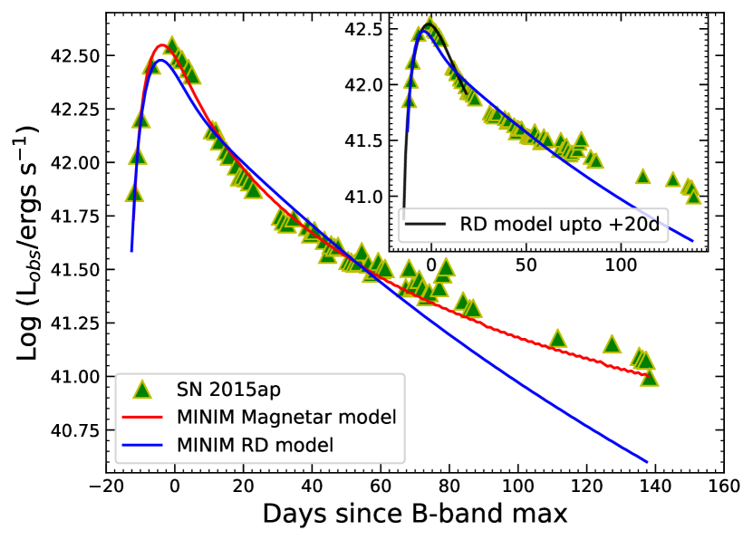
Figure 18: MINIM modelling of the quasi-bolometric light curve of SN 2015ap. The inset shows the RD model fitting only for the early phase (up to +20 d).

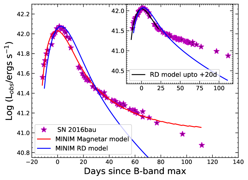
Figure 19: MINIM modelling of the quasi-bolometric light curve of SN 2016bau. The figure in the inset shows the RD model fitting only for the early phase (up to +20 d).

5.1 SN 2015ap

Figure 18 shows the results of RD and MAG model fittings to the quasi-bolometric light curve of SN 2015ap. All of the fitted and calculated parameters are listed in Tables 1 and 2. The ejecta mass ($M_{\rm ej}$) in the RD and MAG models was calculated using Equation 1 from Wheeler et al. (2015). Although the RD model seems to reasonably fit the observed quasi-bolometric light curve, it seems unable to reproduce not only the observed peak luminosity, but also the light curve at late phases, after +50 d. The nickel mass and ejecta mass obtained from these models are somewhat smaller than the ones inferred directly from the observed rise time and peak luminosity in Sec.3.1.3. As the RD model is the prominent powering mechanism for normal SNe Ib, we tried to fit the RD model only up to a relatively early phase ($\sim+20$ d). We see in the inset of Figure 18 that the early phase is nicely fitted in this case. A nickel mass ($M_{\rm Ni}$) of $0.181\pm 0.006\,M_{\odot}$ and an ejecta mass ($M_{\rm ej}$) of $2.1\pm 0.09\,M_{\odot}$ obtained through this fitting are close to the observed values listed in Sec.3.1.3. The fitted and calculated values from the photospheric phase are collected in Table 1.

The MAG model fits the whole observed light curve, both around peak brightness as well as during the late phase, better than the RD model. However, the fitted parameters seem to be unphysical, particularly the very slow initial rotation ($P_{i}\approx 40$ ms) and the very low initial rotational energy ($E_{p}\approx 10^{49}$ erg). This is not surprising given that the magnetar model contains two timescales, one for the rising part and another for the declining part of the light curve (Chatzopoulous et al., 2013). Thus, the possibility of SN 2015ap powered by spin-down of a magnetar is less likely.

5.2 SN 2016bau

Figure 19 shows the results of the RD and MAG model fittings to the quasi-bolometric light curve of SN 2016bau. The fitted and calculated parameters are listed in Tables 1 and 2. The RD model can fit the observed peak luminosity, but huge deviations from the observed light curve are seen in the later phases. The model also fails to match the observed stretch factor of the light curve. Like in the case of SN 2015ap, we also tried to fit only the early part, before +20 d post-peak (see the inset in Fig. 19). In this case, the fitted parameters, such as the nickel mass of $0.065\pm 0.002\,M_{\odot}$ and the ejecta mass of $1.81\pm 0.07\,M_{\odot}$ (see Table 1), are very close to the observed values in Section 3.2.3. Similar to SN 2015ap, the slow rotation ($P_{i}\approx 70$ ms), low magnetar rotational energy ($E_{p}\approx 10^{48}$ erg), and very high progenitor radius ($\sim 1200\,R_{\odot}$) make the MAG model physically unrealistic for SN 2016bau, despite the better fit to the whole light curve in Figure 19.

5.3 Summary of MINIM modelling

The failure of the semi-analytical RD models to simultaneously fit the early and late parts of the light curves of SN 2015ap and SN 2016bau highlights the issues related to the validity of such kinds of models in the case of stripped-envelope SNe. The difficulty in explaining the late-phase decline rate with the assumed diffusion model have already been explored by Wheeler et al. (2015).

Figures 18 and 19 reveal another issue: the model light curve is steeper after +30–40 d than the observed one. This indicates that the early- and late-phase data cannot be fitted simultaneously with the same model parameters. Even though the nickel mass of the second model fits (insets in Figs. 18 and 19) the observed peak luminosity, the decline rate, which is related to the ejecta mass (see Eq. 1 of Wheeler et al. (2015)) is clearly too fast, suggesting an underestimated $M_{\rm ej}$.

This issue is very probably related to the assumption of the constant ejecta density profile (and also the constant opacity). The less steep late part of the light curve needs more ejecta mass to trap the heating gamma-rays originating from the Ni and Co decay. The early part, however, suggests ejecta that dilute much faster than what can fit the late part. Within the context of the constant-density model, this dichotomy means that fitting only the early part results in a lower ejecta mass compared to fitting only the late part (Fig.20).

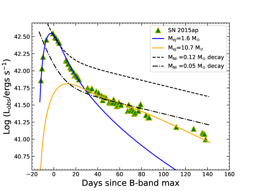
Figure 20: Detailed MINIM modelling to the quasi-bolometric light curve of SN 2015ap. All of the models with different $M_{\rm ej}$ and $M_{\rm Ni}$ are shown together. The models with $M_{\rm ej}=1.6\,M_{\odot}$ and 10.7 $M_{\odot}$ show the RD model fittings considering only the early- and late-phase data, respectively. The other two models show the effect of the amount of nickel present.

Since this issue cannot be solved self-consistently with the constant-density model, and it can plague the mass estimates that consider only the early or late part of the light curve, we investigate it further in the following sections by applying more realistic models for the progenitors and the SN light curves.

6 MESA modelling of a 12 $M_{\odot}$ ZAMS progenitor star

Adoption of a 12 $M_{\odot}$ ZAMS progenitor star for SN 2015ap is primarily based on the results of comparison of the three models from Jerkstrand (2015) and also in the literature; in addition, it supports the observed amount of ejecta mass for SN 2015ap. The ejecta mass for SN 2016bau was calculated to be $\sim 1.6\,M_{\odot}$. On account of such an ejecta mass and the result of Jerkstrand (2015) spectral model matching, we also choose a 12 $M_{\odot}$ ZAMS star as a possible progenitor for SN 2016bau.

We first evolve the 12 $M_{\odot}$ ZAMS star until the onset of core-collapse, using the one-dimensional stellar evolution code MESA, version 11701(Paxton et al., 2011, 2013, 2015, 2018). We do not consider rotation and assume an initial metallicity of $Z=0.02$. Convection is modelled using the mixing theory of Henyey et al. (1965), adopting the Ledoux criterion. We set the mixing-length parameters to $\alpha=3.0$ in the region where the mass fraction of hydrogen is greater than 0.5, and set it to 1.5 in the other regions. Semi-convection is modelled following Langer et al. (1985) with an efficiency parameter of $\alpha_{\mathrm{sc}}=0.01$. For the thermohaline mixing, we follow Kippenhahn et al. (1980), and set the efficiency parameter as $\alpha_{\mathrm{th}}=2.0$. We model the convective overshooting with the diffusive approach of Herwig (2000), with $f=0.01$ and $f_{0}=0.004$ for all the convective core and shells. We use the Dutch scheme for the stellar wind, with a scaling factor of 1.0. The Dutch wind scheme in MESA combines results from several papers. Specifically, when $T_{\mathrm{eff}}>10^{4}$ K and the surface mass fraction of hydrogen is greater than 0.4, the results of Vink et al. (2001) are used, and when $T_{\mathrm{eff}}>10^{4}$ K and the surface mass fraction of hydrogen is less than 0.4, the results of Nugis & Lamers (2000) are used. In the case when $T_{\mathrm{eff}}<10^{4}$ K, the de Jager et al. (1988) wind scheme is used.

SNe Ib have been considered to originate from massive stars which lose almost all of their hydrogen envelope, most probably due to binary interaction (e.g., Yoon et al., 2010; Dessart et al., 2012; Eldridge & Maund, 2016; Ouchi & Maeda, 2017). Here, in order to produce such a stripped model, we artificially strip the hydrogen envelope, mimicking the binary interaction. Specifically, after evolving the model until the exhaustion of helium, we impose an artificial mass-loss rate of $\dot{M}\gtrsim 10^{-4}\,M_{\odot}\,\mathrm{yr}^{-1}$ until the total hydrogen mass of the star goes down to 0.01 $M_{\odot}$. After the hydrogen mass reaches the specified limit, we switch off the artificial mass loss and evolve the model until the onset of core-collapse. At the time of core-collapse, our model has a total mass of $3.42\,M_{\odot}$.

7 Explosions of modelled progenitors using SNEC and STELLA

In this section we briefly discuss the assumptions and setups to produce artificial explosions using SNEC (Morozova et al., 2015) and STELLA (Blinnikov et al., 1998, 2000; Branch et al., 2006) for SN 2015ap and SN 2016bau.

7.1 SN 2015ap

Using the progenitor model on the verge of core-collapse obtained through MESA, we then carried out the radiation hydrodynamical simulations. For this purpose, we use the publicly available codes SNEC and STELLA.

SNEC is a one-dimensional Lagrangian hydrodynamic code, which also solves radiation energy transport with the flux-limited diffusion approximation. The code generates the bolometric light curve and the photospheric velocity evolution of the SN, along with other observed parameters. The setup for the calculation using SNEC closely follows Ouchi & Maeda (2019). Here, we briefly summarise the important parameters and modifications made to Ouchi & Maeda (2019). First, we excise the innermost $1.4\,M_{\odot}$ before the explosion, assuming that it collapses to form a neutron star. The number of cells is set to be 70. Although this number is relatively small, we have confirmed that the light curve and photospheric velocity of the SN are well converged in the time domain of interest. We tried following two possible powering mechanisms for SN 2015ap using SNEC, as follows.

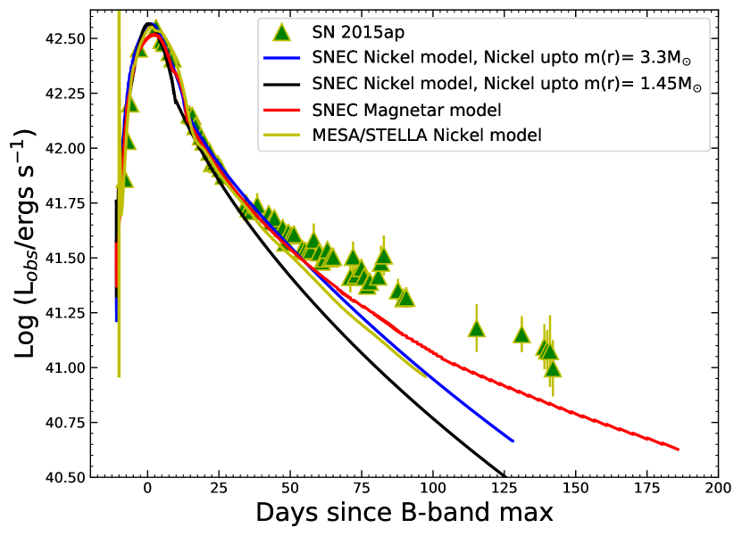
Figure 21: Comparison of quasi-bolometric light curve of SN 2015ap with those obtained using SNEC by taking into account the Ni and Co decay model and the magnetar model. This figure also depicts the result of the Ni–Co decay model obtained using STELLA.

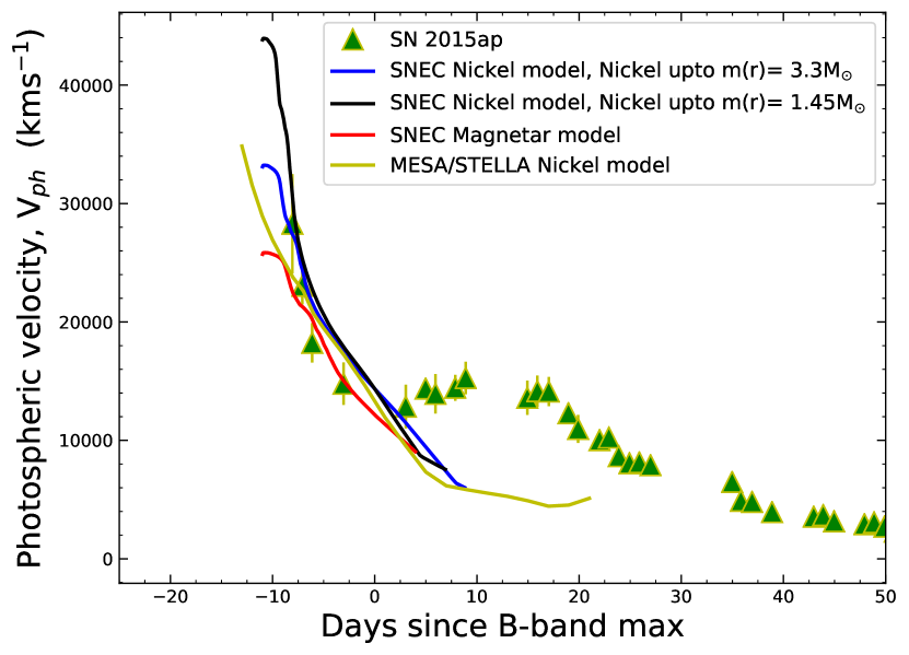
Figure 22: Comparison of the observed velocity evolution of SN 2015ap with that produced by SNEC using two models. We also show a comparison of the observed velocity evolution produced with STELLA.

7.1.1 Ni–Co Decay

The radioactive decay of Ni and Co is considered to be the most prominent mechanism for the powering of light curves of SNe Ib (e.g., Karamehmetoglu, 2017). SNEC incorporates this model by default. Here, we provide the setup of the explosion parameters to incorporate the Ni–Co decay model. The code does not include a nuclear-reaction network, and ⁵⁶Ni is given by hand. We considered two scenarios of nickel distribution. In one case, the mass of Ni is set to be $M_{\mathrm{Ni}}=0.135\,M_{\odot}$ and distributed from the inner boundary up to the mass coordinate $m(r)=3.3\,M_{\odot}$. For this model the explosion is simulated as a piston, with the first two computational cells of the profile boosted outward with a velocity of $4.0\times 10^{9}$ cm s^-1 for a time interval of 0.01 s. The total energy ($E_{\rm tot}$) of the model is $3.7\times 10^{51}$ erg. For the second case, the mass of Ni is set to be $M_{\mathrm{Ni}}=0.1\,M_{\odot}$ and distributed near the centre, from the inner boundary up to the mass coordinate of $m(r)=1.45\,M_{\odot}$. The explosion is simulated as a piston, with the first two computational cells of the profile boosted outward with a velocity of $5.0\times 10^{9}$ cm s^-1 for a time interval of 0.01 s. The total energy of the model in this case is $6.5\times 10^{51}$ erg. Thus, our results provide a range of $M_{\mathrm{Ni}}$ and total energy, depending on the distribution of nickel mass.

7.1.2 Spin-down of a magnetar

We also tried a magnetar-powering mechanism for the light curve as SN 2015ap; it shows some resemblance to SN 2008D, which has broader features in its early-time spectra and also some X-ray emission in the later phases. A few SNe Ib are also explained by magnetar models, one such example being SN 2005bf (Maeda et al., 2007). For this model, the explosion is the piston type, with the first two computational cells of the profile boosted outward with a velocity of $3.3\times 10^{9}$ cm s^-1 for a time interval of 0.01 s. The total energy of the model in this case is $2.2\times 10^{51}$ erg. The most important change made to Ouchi & Maeda (2019) is that we add the magnetar heat to the ejecta.

Following Metzger et al. (2015), the magnetar spin-down luminosity is given by

$$L_{\mathrm{sd}}=L_{\mathrm{sd_{i}}}(1+t/t_{\mathrm{sd}})^{-2}.$$

Here, $L_{\mathrm{sd_{i}}}$ is the spin-down luminosity at $t=0$, and $t_{\mathrm{sd}}$ is the initial spin-down time. We inject this luminosity into the whole ejecta above the mass cut uniformly in mass. For the initial spin-down luminosity, we assume $L_{\mathrm{sd{{}_{i}}}}=1.3\times 10^{43}$ erg s^-1, while for the initial spin-down time, we assume $t_{\mathrm{sd}}=12$ d. In this model, we do not include the effect of Ni heating. Following Metzger et al. (2015) (Equations 2 and 3), corresponding to $L_{\mathrm{sd{{}_{i}}}}=1.3\times 10^{43}$ erg s^-1 and $t_{\mathrm{sd}}=12$ d, we obtain a magnetic field ($B$) of $5.1\times 10^{14}$ G and an initial period ($P_{i}$) of 43.06 ms for the modelled magnetar. These values of $B$ and $P_{i}$ are very close to those obtained using MINIM.

We also use the public version of STELLA, available with MESA. The default radioactive decay of ⁵⁶Ni and ⁵⁶Co as a powering mechanism is used for SN 2015ap. Nearly similar parameters as in the case of SNEC are used for STELLA. The MESA setups are unchanged for STELLA calculations. We use a total energy after explosion of $3.6\times 10^{51}$ erg and a ⁵⁶Ni mass of $0.193\,M_{\odot}$, which is slightly more than the ⁵⁶Ni mass used in SNEC. In order to avoid the numerical problem caused by the high-velocity material, we removed the outer layer of the progenitor where the density is less than $10^{-5}$ g cm^-3 (see also Moriya et al., 2020).

7.1.3 Summary of the modelling

Figure 21 shows the comparison of the observed quasi-bolometric luminosity with that produced by SNEC. We find that the radioactive decay models with ⁵⁶Ni mass in the range 0.1–0.135 $M_{\odot}$ and total energy in the range (3.7–6.5) $\times 10^{51}$ erg could nicely explain the light curve. Our results also signify that the distribution of ⁵⁶Ni mass plays an important role for explaining the observed light curves. The magnetar model could also explain the quasi-bolometric light curve, but we do not see very strong evidence that SN 2015ap is powered by a magnetar. This figure also shows the results of STELLA calculations. We see that, although the explosion energy is similar, we need a slightly higher amount of nickel to properly match the observed light curve of SN 2015ap.

Figure 22 illustrates a comparison of observed photospheric velocity evolution produced by blackbody fitting with that produced by SNEC. We see that the Ni–Co decay and magnetar models initially show higher velocities, but in the later epochs they well replicate the observed photospheric velocities. This figure also shows the Fe II 5169 $\mathrm{\SIUnitSymbolAngstrom}$ velocity evolution produced by STELLA. Owing to the unambiguous absence of Fe II 5169 $\mathrm{\SIUnitSymbolAngstrom}$ features in SN 2015ap, we used the photospheric velocity obtained through a blackbody fit for our comparison of Fe II 5169 $\mathrm{\SIUnitSymbolAngstrom}$ line velocities. We can see a very good match between the STELLA velocities and observed ones. The modelling parameters, along with the observed values, are listed in Table 3.

7.2 SN 2016bau

Using a similar progenitor model on the verge of core-collapse, obtained through MESA, as in the case of SN 2015ap, we carried out the radiation hydrodynamical simulations using SNEC and STELLA. For calculations using SNEC, the setup closely follows that of Ouchi & Maeda (2019). First, we excise the innermost $1.53\,M_{\odot}$ before the explosion, assuming that it collapses to form a neutron star. The number of cells is set to 70. We try two possible powering mechanisms for SN 2016bau using SNEC, as follows.

Table 3: Observed and modelled parameters for SN 2015ap and SN 2016bau

	$M_{\mathrm{Ni}}$	$M_{\mathrm{ej}}$	$E_{\mathrm{tot}}$
	($M_{\odot}$)	($M_{\odot}$)	$10^{51}$ erg
SN 2015ap
Arnett’s modela	0.14 $\pm$ 0.02	2.2 $\pm$ 0.6	*
SNEC (Ni distributed up to $M(r)=3.3\,M_{\odot}$)	0.135	2.02	3.7
SNEC (Ni distributed up to $M(r)=1.45\,M_{\odot}$)	0.1	2.02	6.5
SNEC Magnetar model	0.0	2.02	2.2
From STELLA	0.193	1.92	3.6
SN 2016bau
Arnett’s modela	0.055 $\pm$ 0.006	1.6 $\pm$ 0.3	**
SNEC (Ni distributed up to $M(r)=3.3\,M_{\odot}$)	0.045	1.89	1.23
SNEC (Ni distributed up to $M(r)=1.57\,M_{\odot}$)	0.03	1.89	1.93
SNEC Magnetar model	0.0	1.89	0.8
From STELLA	0.065	1.89	1.6

$a$: Calculated using $t_{\rm rise}$, $\kappa=0.07$ cm² g^-1, and $L_{\rm peak}$.
$*$: Instead, a kinetic energy of the ejecta $(E_{k})=1.05\times 10^{51}$ erg is obtained.
$**$: Instead, a kinetic energy of the ejecta $(E_{k})=0.24\times 10^{51}$ erg is obtained.

7.2.1 Ni–Co Decay

The setup for the calculation using SNEC is similar to that of SN 2015ap. Considering the radioactive decay of Ni–Co the most prominent mechanism for powering light curves of SNe Ib, we employed this model as the powering mechanism for SN 2016bau. Here we briefly describe the setup of the explosion parameters incorporated in the Ni–Co decay model.

We considered two cases of ⁵⁶Ni mass distribution. In the first case, the mass of ⁵⁶Ni synthesised is set to be $M_{\mathrm{Ni}}=0.045\,M_{\odot}$. Then, it is distributed from the inner boundary up to the mass coordinate of $M(r)=3.3\,M_{\odot}$. Thereafter, we simulate the explosion as a piston, with the first two computational cells of the profile boosted outward with a velocity of $4.2\times 10^{9}$ cm s^-1 for a time interval of 0.01 s. The model has a total energy of $1.3\times 10^{51}$ erg. For the second case, the mass of ⁵⁶Ni synthesised is set to be $M_{\mathrm{Ni}}=0.03\,M_{\odot}$ and distributed from the inner boundary up to the mass coordinate of $M(r)=1.57\,M_{\odot}$. Thereafter, we simulate the explosion as a piston, with the first two computational cells of the profile boosted outward with a velocity of $4.9\times 10^{9}$ cm s^-1 for a time interval of 0.01 s, and the model has a total energy of $1.93\times 10^{51}$ erg. We find that, depending on the $M_{\mathrm{Ni}}$ distribution, the radioactive decay models with ⁵⁶Ni mass in the range 0.03–$0.045\,M_{\odot}$ and total energy in the range (1.23–1.93) $\times 10^{51}$ erg can nicely explain the light curve.

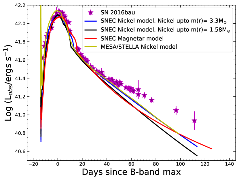
Figure 23: Comparison of the quasi-bolometric light curve of SN 2016bau and light curves produced by SNEC and STELLA, considering the radioactive decay model.

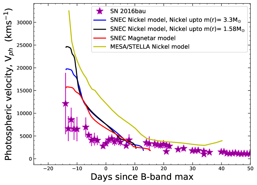
Figure 24: Comparison between the observed velocity evolution of SN 2016bau and the photometric velocity evolution produced by SNEC and STELLA, considering the radioactive decay model.

7.2.2 Spin-down of a magnetar

We also tried the magnetar powering mechanism for SN 2016bau. The explosion is simulated as a piston, with the first two computational cells of the profile boosted outward with a velocity of $3.6\times 10^{9}$ cm s^-1 for a duration of 0.01 s and a total model energy of $0.8\times 10^{51}$ erg. Like SN 2015ap, we inject $L_{\mathrm{sd_{i}}}=0.4\times 10^{43}$ erg s^-1 to the ejecta above the mass cut uniformly in mass. We assume $t_{\mathrm{sd}}=16.0$ d and do not include the effect of Ni heating. Corresponding to $L_{\mathrm{sd{{}_{i}}}}=0.4\times 10^{43}$ erg s^-1 and $t_{\mathrm{sd}}=16$ d, we obtain a magnetic field ($B$) of $7.9\times 10^{14}$ G and an initial period ($P_{i}$) of 71.8 ms for the modelled magnetar. These values of $B$ and $P_{i}$ are very close to those obtained using MINIM.

We also perform STELLA calculations for SN 2016bau, by employing the default radioactive decay of ⁵⁶Ni and ⁵⁶Co powering mechanism. We used similar parameters as in the case of SNEC and STELLA. The MESA setups are unchanged for STELLA calculations. We used a total energy after explosion of $1.6\times 10^{51}$ erg and a ⁵⁶Ni mass of $0.065\,M_{\odot}$, slightly above the ⁵⁶Ni mass used in SNEC.

7.2.3 Summary of the modelling

Figure 23 shows the comparison of the observed quasi-bolometric luminosity with that produced by SNEC for the radioactive decay and magnetar spin-down models. We find that the radioactive decay model from SNEC could successfully explain the light curve. The magnetar model also shows a good match, but we do not see any significant signs of SN 2016bau being powered by a magnetar. This figure also shows the results of STELLA calculations; they also match the observed light curve of SN 2016bau nicely, with parameters similar to those of SNEC.

Figure 24 shows a comparison of the observed photospheric velocity evolution produced by blackbody fitting with that produced by the radioactive decay model and the magnetar spin-down model using SNEC. Here, the models show high initial velocities which drop at later epochs. We see that the velocities produced by the models initially deviate from the observed photospheric velocities, but tend to follow velocities similar to the observed ones at later epochs. The figure also shows a comparison the Fe II 5169 $\mathrm{\SIUnitSymbolAngstrom}$ line velocity obtained using STELLA with the photospheric velocity obtained through blackbody fits. Similar to the case of SN 2015ap, this SN also lacks unambiguous features of the Fe II 5169 $\mathrm{\SIUnitSymbolAngstrom}$ line.

From Figure 24, it is evident that our model overestimates the velocity by a factor of nearly two. The $M_{\rm ej}$ from Arnett’s model is $\sim 1.6\,M_{\odot}$. The diffusion time is given by $(M^{3}/E)^{1/4}$. Since this combination is fixed, $M^{3}/E$ is roughly constant. But $M^{3}/E\approx M^{3}/(Mv^{2})=M^{2}/v^{2}\approx$ constant. Thus, we have $M\approx v$ to meet the observational constraints. So, if we need to decrease the velocity by a factor of two, the ejecta mass would also decrease by the same factor. Then the He star mass is likely $\sim 2$–2.5 $M_{\odot}$, which is at the boundary between a SN and a non-SN. Since $E\approx Mv^{2}\approx v^{3}$, the energy may go down quite substantially in this case.

8 Discussion

We present a detailed photometric and spectroscopic analysis of two Type Ib SNe, namely SN 2015ap and SN 2016bau. From our analysis, SN 2015ap is an intermediate-luminosity normal SN Ib, while SN 2016bau is highly extinguished by host-galaxy dust. In this section, we discuss the major outcomes of our present analysis.

The photometric properties of both the SNe were analysed by determining the bolometric luminosity of their light curves. For SN 2015ap, we calculate a ⁵⁶Ni mass of $0.14\pm 0.02$ $M_{\odot}$ and an ejecta mass of $2.2\pm 0.6$ $M_{\odot}$, while for SN 2016bau, the ⁵⁶Ni mass and ejecta mass were $0.055\pm 0.006\,M_{\odot}$ and $1.6\pm 0.3\,M_{\odot}$, respectively. The photospheric temperature, radius, and velocity evolution for both SNe were also explored. Based on the derived physical quantities from the temporal evolution of these two SNe, we tried to constrain possible powering mechanisms using a semi-analytical model called MINIM. We found that the semi-analytical RD model failed to simultaneously fit the early and late phases of both SNe, raising issues related to the validity of such models in the case of stripped-envelope SNe. One solution to such a situation is to fit the early-phase and late-phase data with different sets of model parameters. Another cause for the failure of the RD model can be attributed to the assumption of the constant ejecta density profile. For the MAG model, the fitted parameters seemed to be unphysical in both SNe, especially the very slow initial rotation (for SN 2015ap, $P_{i}\approx 40$ ms, and for SN 2016bau, $P_{i}\approx 70$ ms) and the very low initial rotational energy (for both SNe, $E_{p}\approx 10^{49}$ erg). Also, no signs of these SNe powered by a magnetar mechanism were evident either from photometry or spectroscopy, so this possibility was discarded.

The spectroscopic behaviour of both SNe was also studied using the present and archival data. These SNe showed unambiguous He I features from very early to late phases, confirming them to be SNe Ib. Their spectral features match with those of other well-studied SNe Ib. Additionally, SN 2015ap closely resembled SN 2008D, which had shown X-ray emission. The spectra of our two SNe at various epochs were modelled using SYN++. For SN 2015ap, the spectral modelling indicated a range of photospheric temperatures and velocities from 13,000 km s^-1 to 6800 km s^-1 and from 12,000 K to 4500 K (respectively) during the time interval $-7$ d to +33 d. For SN 2016bau, these two parameters ranged from 16,000 km s^-1 to 8000 km s^-1 and from 9000 K to 4000 K (respectively) during the time interval $-14$ d to +33 d. The spectra of these two SNe at particular epochs were compared with model spectra of 12, 13, and 17 $M_{\odot}$ progenitor stars. For SN 2015ap, the 12 $M_{\odot}$ and 17 $M_{\odot}$ model spectra showed reasonable matches, indicating a progenitor in the mass range 12–17 $M_{\odot}$; for SN 2016bau, the 12 M_⊙ model spectrum could explain the observed spectrum to some extent better than other models, indicating a $\leq 12\,M_{\odot}$ progenitor.

Based on the photometric and spectroscopic properties described above, a 12 $M_{\odot}$ ZAMS star was chosen as the possible progenitor for both SNe. This 12 $M_{\odot}$ ZAMS progenitor was evolved up to the onset of core collapse using MESA. The MESA outputs on the onset of core collapse were fed as input to SNEC and STELLA, which simulate the synthetic explosions. The RD and MAG models were employed using SNEC while only the RD model was employed in STELLA. Here also, the models failed to fit the late part of the light curve simultaneously. The cause can be attributed to the various assumptions, including the spherically symmetrical explosions and the use of constant ejecta density profiles throughout. Similar to the case of MINIM, the MAG model provided unphysical parameters during the SNEC analysis.

Our analysis favours a 12 $M_{\odot}$ ZAMS star as a possible progenitor for SN 2015ap based on outputs of the models reasonably explaining the bolometric luminosity light curve and the photospheric velocity. However, in case of SN 2016bau, the model velocities are higher by a factor of almost 2, demanding that the ejecta mass be lower by similar factor. This would imply an He star of mass $\sim 2$–2.5 $M_{\odot}$, which is at the boundary for exploding as an SN. Thus, a slightly lower mass ZAMS star could also be the possible progenitor of SN 2016bau. Hydrodynamical evolution models of such low-mass stars to reach the stage of core collapse and then undergo synthetic explosions are extremely difficult to perform, but this can be taken as a challenge for the future.

9 Conclusions

Photometric and spectroscopic analyses of the Lick/KAIT-discovered Type Ib SN 2015ap and another Type Ib SN 2016bau, both having extensive follow-up observations made with various telescopes, are discussed. For both SNe, photometric data corrected for the Milky Way and host-galaxy extinction were used to estimate the quasi-bolometric luminosity light curves and study the photospheric radius, temperature, and velocity evolution. Spectral properties of SN 2015ap and SN 2016bau were then explored in detail. We modelled the spectra, studied the spectral evolution, and compared the spectra at various epochs with those of other well-studied SNe Ib, which further confirmed that these two SNe are Type Ib SN.

We attempted to determine the progenitor masses of SN 2015ap and SN 2016bau. Our results support $12\,M_{\odot}$ progenitors for these two SNe. The $12\,M_{\odot}$ ZAMS progenitor was evolved up to the onset of core-collapse using MESA. The output of MESA was incorporated as input to SNEC and STELLA, which produced the artificial explosions replicating the actual SN explosions. Considering the decay of Ni and Co to be the most prominent powering mechanism for SNe Ib, we tried this powering mechanism for SN 2015ap and SN 2016bau, using SNEC and STELLA. We found that the quasi-bolometric luminosity could nicely be explained by our models, while the velocity evolution obtained from SNEC and STELLA satisfactorily agrees with the observed one. We also explored the effect of the distribution of nickel mass near the centre and up to near the surface. Lower amounts of nickel were required to match the light curve for the case of centrally distributed nickel in comparison to the case where the nickel was distributed up to near the surface. Based on the above conclusions, our analysis supports a star having $M_{\rm ZAMS}=12\,M_{\odot}$ as the possible progenitor for SN 2015ap. For SN 2016bau, a slightly lower ZAMS progenitor is expected.

Data availability

The photometric and spectroscopic data used in this work can be made available on request to the corresponding author. The inlist files to create the MESA models and STELLA calculations, along with SNEC parameters files, can also be made available on request to the corresponding author.

Appendix A Log of spectroscopic and photometric observations

Table 4: Spectroscopic observations of SN 2016bau.

Note: All spectra were taken with the Kast spectrograph on the 3.0 m Shane telescope at Lick Observatory.

UT Date	MJD
2016/03/16	57463.719
2016/03/19	57466.919
2016/04/03	57481.671
2016/04/17	57495.902
2016/05/02	57510.671
2016/05/16	57524.860
2016/05/30	57538.741
2016/07/15	57584.710

Table 5: Photometry of SN 2015ap.

MJD	$B$	$V$	$R$	$I$	Telescope
	(mag)	(mag)	(mag)	(mag)	(mag)
57274.4258	17.35 $\pm$ 0.09	17.28 $\pm$ 0.07	17.07 $\pm$ 0.05	16.75 $\pm$ 0.06	KAIT
57275.3867	16.94 $\pm$ 0.09	16.83 $\pm$ 0.06	16.67 $\pm$ 0.05	16.39 $\pm$ 0.06	KAIT
57276.3516	16.40 $\pm$ 0.17	16.40 $\pm$ 0.11	16.39 $\pm$ 0.08	16.05 $\pm$ 0.07	KAIT
57279.4336	15.79 $\pm$ 0.11	15.84 $\pm$ 0.06	15.64 $\pm$ 0.05	15.39 $\pm$ 0.05	KAIT
57283.4375	15.44 $\pm$ 0.01	15.26 $\pm$ 0.01	15.14 $\pm$ 0.01	14.93 $\pm$ 0.01	Nickel
57285.5078	15.64 $\pm$ 0.08	15.44 $\pm$ 0.04	15.20 $\pm$ 0.03	14.90 $\pm$ 0.03	KAIT
57286.4062	15.70 $\pm$ 0.04	15.48 $\pm$ 0.03	15.14 $\pm$ 0.02	14.87 $\pm$ 0.02	KAIT
57287.4375	15.91 $\pm$ 0.05	15.47 $\pm$ 0.03	15.18 $\pm$ 0.03	14.87 $\pm$ 0.03	KAIT
57288.4102	15.89 $\pm$ 0.05	15.51 $\pm$ 0.03	15.17 $\pm$ 0.03	14.86 $\pm$ 0.03	KAIT
57290.3555	16.07 $\pm$ 0.07	15.55 $\pm$ 0.05	15.20 $\pm$ 0.03	14.87 $\pm$ 0.03	KAIT
57291.3594	16.30 $\pm$ 0.09	15.58 $\pm$ 0.04	15.19 $\pm$ 0.03	14.88 $\pm$ 0.013	KAIT
57297.4023	17.06 $\pm$ 0.20	16.27 $\pm$ 0.07	15.71 $\pm$ 0.04	15.19 $\pm$ 0.04	KAIT
57298.3906	17.30 $\pm$ 0.12	16.20 $\pm$ 0.04	15.75 $\pm$ 0.03	15.23 $\pm$ 0.03	KAIT
57299.5039	17.35 $\pm$ 0.15	16.53 $\pm$ 0.05	15.91 $\pm$ 0.03	15.22 $\pm$ 0.03	KAIT
57301.4258	17.52 $\pm$ 0.11	16.48 $\pm$ 0.04	15.98 $\pm$ 0.03	15.35 $\pm$ 0.03	KAIT
57302.3125	17.43 $\pm$ 0.01	16.37 $\pm$ 0.01	15.86 $\pm$ 0.01	15.33 $\pm$ 0.01	Nickel
57302.3672	17.47 $\pm$ 0.08	16.52 $\pm$ 0.04	16.05 $\pm$ 0.03	15.46 $\pm$ 0.03	KAIT
57304.4727	17.68 $\pm$ 0.12	16.76 $\pm$ 0.07	16.19 $\pm$ 0.04	15.57 $\pm$ 0.03	KAIT
57305.3828	17.90 $\pm$ 0.12	16.76 $\pm$ 0.05	16.27 $\pm$ 0.03	15.61 $\pm$ 0.03	KAIT
57306.3516	17.88 $\pm$ 0.18	16.84 $\pm$ 0.06	16.26 $\pm$ 0.04	15.65 $\pm$ 0.04	KAIT
57307.3438	17.74 $\pm$ 0.01	16.72 $\pm$ 0.01	16.18 $\pm$ 0.01	15.63 $\pm$ 0.01	Nickel
57307.3945	17.82 $\pm$ 0.13	16.86 $\pm$ 0.04	16.27 $\pm$ 0.03	15.76 $\pm$ 0.04	KAIT
57308.3633	17.82 $\pm$ 0.12	16.83 $\pm$ 0.05	16.34 $\pm$ 0.03	15.75 $\pm$ 0.04	KAIT
57309.4609	17.91 $\pm$ 0.16	16.89 $\pm$ 0.08	16.35 $\pm$ 0.04	15.73 $\pm$ 0.04	KAIT
57317.3047	17.98 $\pm$ 0.02	17.10 $\pm$ 0.01	16.64 $\pm$ 0.01	15.99 $\pm$ 0.01	Nickel
57317.4492	18.31 $\pm$ 0.24	17.25 $\pm$ 0.08	16.75 $\pm$ 0.05	16.02 $\pm$ 0.04	KAIT
57318.3008	18.19 $\pm$ 0.27	17.30 $\pm$ 0.09	16.72 $\pm$ 0.05	16.12 $\pm$ 0.05	KAIT
57319.3984	18.22 $\pm$ 0.20	17.48 $\pm$ 0.12	16.80 $\pm$ 0.05	16.12 $\pm$ 0.07	KAIT
57325.4297	18.25 $\pm$ 0.38	17.14 $\pm$ 0.14	17.15 $\pm$ 0.09	16.19 $\pm$ 0.07	KAIT
57326.3594	18.42 $\pm$ 0.29	17.43 $\pm$ 0.07	17.03 $\pm$ 0.05	16.35 $\pm$ 0.04	KAIT
57327.4297	17.98 $\pm$ 0.26	17.40 $\pm$ 0.12	-	-	KAIT
57330.3906	18.37 $\pm$ 0.22	17.58 $\pm$ 0.08	17.20 $\pm$ 0.06	16.46 $\pm$ 0.05	KAIT
57331.3359	18.63 $\pm$ 0.22	17.72 $\pm$ 0.08	17.16 $\pm$ 0.04	16.59 $\pm$ 0.05	KAIT
57332.3047	18.21 $\pm$ 0.01	17.47 $\pm$ 0.01	17.11 $\pm$ 0.01	16.47 $\pm$ 0.01	Nickel
57332.3555	18.31 $\pm$ 0.18	17.57 $\pm$ 0.07	17.21 $\pm$ 0.04	16.56 $\pm$ 0.04	KAIT
57333.3477	18.19 $\pm$ 0.17	17.73 $\pm$ 0.09	17.23 $\pm$ 0.06	16.56 $\pm$ 0.05	KAIT
57334.3789	18.35 $\pm$ 0.16	17.66 $\pm$ 0.08	17.25 $\pm$ 0.06	16.51 $\pm$ 0.05	KAIT
57337.3281	18.33 $\pm$ 0.20	18.01 $\pm$ 0.18	17.33 $\pm$ 0.05	16.85 $\pm$ 0.06	KAIT
57338.2852	18.62 $\pm$ 0.28	17.79 $\pm$ 0.12	17.30 $\pm$ 0.05	16.73 $\pm$ 0.05	KAIT
57339.3125	18.45 $\pm$ 0.22	17.83 $\pm$ 0.08	17.46 $\pm$ 0.05	16.75 $\pm$ 0.06	KAIT
57339.3438	18.28 $\pm$ 0.02	17.64 $\pm$ 0.01	17.27 $\pm$ 0.02	16.66 $\pm$ 0.01	Nickel
57340.3594	18.52 $\pm$ 0.18	17.76 $\pm$ 0.07	17.40 $\pm$ 0.06	16.73 $\pm$ 0.06	KAIT
57343.3906	18.31 $\pm$ 0.02	17.66 $\pm$ 0.01	17.38 $\pm$ 0.02	16.64 $\pm$ 0.01	Nickel
57347.3164	18.51 $\pm$ 0.03	17.73 $\pm$ 0.01	17.51 $\pm$ 0.02	17.02 $\pm$ 0.02	Nickel
57361.2656	18.55 $\pm$ 0.02	18.14 $\pm$ 0.01	17.93 $\pm$ 0.02	17.19 $\pm$ 0.01	Nickel
57425.1641	19.22 $\pm$ 0.06	19.63 $\pm$ 0.07	-	-	Nickel
57431.1250	19.51 $\pm$ 0.10	19.48 $\pm$ 0.10	19.05 $\pm$ 0.34	-	Nickel
57444.1328	19.67 $\pm$ 0.09	20.06 $\pm$ 0.10	19.82 $\pm$ 0.09	18.93 $\pm$ 0.06	Nickel

Table 6: Log of HST observations of SN 2015ap.

Note: All exposures were 710 s and there were no detections.

UT Date	Filter
2017/08/16	F555W
2017/02/19	F814W
2016/04/03	F555W
2016/04/17	F814W

Table 7: Photometry of SN 2016bau

MJD	$B$	$V$	$R$	$clear$	$I$	Telescope
	(mag)	(mag)	(mag)	(mag)	(mag)
57462.384	-	-	-	16.896 $\pm$ 0.190	-
57463.381	17.196 $\pm$ 0.160	16.691 $\pm$ 0.131	16.488 $\pm$ 0.165	16.553 $\pm$ 0.226	16.381 $\pm$ 0.124	KAIT
57464.338	16.843 $\pm$ 0.119	16.408 $\pm$ 0.080	16.180 $\pm$ 0.102	16.199 $\pm$ 0.103	16.079 $\pm$ 0.086	KAIT
57465.324	16.879 $\pm$ 0.120	16.192 $\pm$ 0.066	16.027 $\pm$ 0.070	15.967 $\pm$ 0.131	15.809 $\pm$ 0.106	KAIT
57466.310	16.726 $\pm$ 0.134	16.005 $\pm$ 0.057	15.852 $\pm$ 0.055	15.838 $\pm$ 0.105	15.661 $\pm$ 0.063	KAIT
57467.330	16.787 $\pm$ 0.253	15.890 $\pm$ 0.103	15.608 $\pm$ 0.098	15.767 $\pm$ 0.156	15.451 $\pm$ 0.128	KAIT
57470.385	16.762 $\pm$ 0.165	15.741 $\pm$ 0.071	15.376 $\pm$ 0.074	15.374 $\pm$ 0.061	15.165 $\pm$ 0.091	KAIT
57471.397	16.401 $\pm$ 0.176	15.589 $\pm$ 0.059	15.278 $\pm$ 0.053	15.288 $\pm$ 0.062	15.114 $\pm$ 0.056	KAIT
57472.397	16.358 $\pm$ 0.140	15.477 $\pm$ 0.061	15.202 $\pm$ 0.051	15.254 $\pm$ 0.065	15.031 $\pm$ 0.055	KAIT
57473.355	16.282 $\pm$ 0.114	15.467 $\pm$ 0.049	15.196 $\pm$ 0.049	15.206 $\pm$ 0.072	14.982 $\pm$ 0.055	KAIT
57474.383	16.106 $\pm$ 0.315	15.464 $\pm$ 0.083	15.107 $\pm$ 0.063	15.154 $\pm$ 0.075	14.882 $\pm$ 0.114	KAIT
57476.373	16.079 $\pm$ 0.131	15.398 $\pm$ 0.048	15.026 $\pm$ 0.049	15.067 $\pm$ 0.079	14.806 $\pm$ 0.052	KAIT
57477.367	16.274 $\pm$ 0.088	15.348 $\pm$ 0.042	15.048 $\pm$ 0.042	15.073 $\pm$ 0.046	14.787 $\pm$ 0.042	KAIT
57478.332	16.340 $\pm$ 0.082	15.376 $\pm$ 0.044	15.005 $\pm$ 0.042	15.055 $\pm$ 0.080	14.744 $\pm$ 0.040	KAIT
57479.395	16.290 $\pm$ 0.123	15.365 $\pm$ 0.054	14.989 $\pm$ 0.053	15.039 $\pm$ 0.089	14.750 $\pm$ 0.060	KAIT
57480.345	16.440 $\pm$ 0.087	15.422 $\pm$ 0.034	15.037 $\pm$ 0.038	15.062 $\pm$ 0.045	14.753 $\pm$ 0.056	KAIT
57481.338	16.487 $\pm$ 0.207	15.444 $\pm$ 0.070	15.102 $\pm$ 0.065	15.105 $\pm$ 0.073	14.713 $\pm$ 0.062	KAIT
57482.341	16.801 $\pm$ 0.142	15.527 $\pm$ 0.053	15.057 $\pm$ 0.045	15.132 $\pm$ 0.065	14.784 $\pm$ 0.049	KAIT
57485.358	17.453 $\pm$ 0.207	15.691 $\pm$ 0.115	15.237 $\pm$ 0.093	15.320 $\pm$ 0.090	15.039 $\pm$ 0.090	KAIT
57491.352	17.914 $\pm$ 0.243	16.282 $\pm$ 0.118	15.730 $\pm$ 0.119	15.744 $\pm$ 0.141	15.224 $\pm$ 0.116	KAIT
57492.352	17.765 $\pm$ 0.159	16.376 $\pm$ 0.103	15.776 $\pm$ 0.085	15.824 $\pm$ 0.137	15.262 $\pm$ 0.073	KAIT
57494.257	17.979 $\pm$ 0.169	16.484 $\pm$ 0.108	15.896 $\pm$ 0.111	15.941 $\pm$ 0.148	15.392 $\pm$ 0.125	KAIT
57495.299	18.142 $\pm$ 0.134	16.553 $\pm$ 0.069	15.914 $\pm$ 0.071	16.018 $\pm$ 0.095	15.427 $\pm$ 0.064	KAIT
57496.272	18.106 $\pm$ 0.131	16.603 $\pm$ 0.065	15.970 $\pm$ 0.063	16.048 $\pm$ 0.093	15.445 $\pm$ 0.058	KAIT
57497.268	18.194 $\pm$ 0.186	16.721 $\pm$ 0.086	15.966 $\pm$ 0.065	16.100 $\pm$ 0.084	15.492 $\pm$ 0.067	KAIT
57498.330	18.137 $\pm$ 0.145	16.646 $\pm$ 0.094	16.065 $\pm$ 0.087	16.129 $\pm$ 0.114	15.557 $\pm$ 0.079	KAIT
57499.317	18.147 $\pm$ 0.329	16.675 $\pm$ 0.149	16.111 $\pm$ 0.141	16.193 $\pm$ 0.230	15.555 $\pm$ 0.131	KAIT
57502.338	18.204 $\pm$ 0.277	16.935 $\pm$ 0.170	16.180 $\pm$ 0.204	16.201 $\pm$ 0.147	15.674 $\pm$ 0.095	KAIT
57504.271	18.340 $\pm$ 0.173	16.893 $\pm$ 0.111	16.291 $\pm$ 0.114	16.313 $\pm$ 0.165	15.738 $\pm$ 0.095	KAIT
57505.327	-	-	-	16.297 $\pm$ 0.148	-	KAIT
57507.265	18.362 $\pm$ 0.179	16.974 $\pm$ 0.109	16.372 $\pm$ 0.116	16.408 $\pm$ 0.184	15.803 $\pm$ 0.089	KAIT
57508.241	18.348 $\pm$ 0.248	16.993 $\pm$ 0.197	16.445 $\pm$ 0.210	16.408 $\pm$ 0.237	15.837 $\pm$ 0.163	KAIT
57509.285	18.414 $\pm$ 0.156	17.023 $\pm$ 0.110	16.401 $\pm$ 0.119	16.441 $\pm$ 0.181	15.825 $\pm$ 0.098	KAIT
57510.229	-	-	-	16.458 $\pm$ 0.172	-	KAIT
57511.236	18.498 $\pm$ 0.154	17.092 $\pm$ 0.121	16.484 $\pm$ 0.086	16.447 $\pm$ 0.178	15.848 $\pm$ 0.087	KAIT
57513.195	18.490 $\pm$ 0.417	17.150 $\pm$ 0.163	16.552 $\pm$ 0.134	16.517 $\pm$ 0.195	15.929 $\pm$ 0.112	KAIT
57517.272	18.501 $\pm$ 0.189	17.238 $\pm$ 0.104	16.619 $\pm$ 0.116	16.594 $\pm$ 0.221	16.001 $\pm$ 0.096	KAIT
57518.210	18.590 $\pm$ 0.151	17.221 $\pm$ 0.129	16.668 $\pm$ 0.114	16.591 $\pm$ 0.139	15.993 $\pm$ 0.094	KAIT
57519.223	18.514 $\pm$ 0.156	17.211 $\pm$ 0.094	16.671 $\pm$ 0.095	16.612 $\pm$ 0.127	16.043 $\pm$ 0.101	KAIT
57520.193	18.453 $\pm$ 0.167	17.284 $\pm$ 0.148	16.669 $\pm$ 0.099	16.651 $\pm$ 0.349	16.039 $\pm$ 0.102	KAIT
57521.203	18.651 $\pm$ 0.179	17.276 $\pm$ 0.126	16.737 $\pm$ 0.121	16.699 $\pm$ 0.119	16.057 $\pm$ 0.093	KAIT
57522.186	18.638 $\pm$ 0.215	17.359 $\pm$ 0.186	16.744 $\pm$ 0.190	16.727 $\pm$ 0.263	16.074 $\pm$ 0.155	KAIT
57523.259	18.510 $\pm$ 0.235	17.396 $\pm$ 0.194	16.697 $\pm$ 0.149	16.672 $\pm$ 0.322	16.029 $\pm$ 0.118	KAIT
57524.206	18.643 $\pm$ 0.147	17.346 $\pm$ 0.121	16.717 $\pm$ 0.116	16.753 $\pm$ 0.229	16.068 $\pm$ 0.102	KAIT
57525.193	18.675 $\pm$ 0.168	17.392 $\pm$ 0.090	16.802 $\pm$ 0.118	16.729 $\pm$ 0.134	16.117 $\pm$ 0.110	KAIT
57526.218	18.464 $\pm$ 0.205	17.358 $\pm$ 0.120	16.748 $\pm$ 0.113	16.739 $\pm$ 0.243	16.097 $\pm$ 0.101	KAIT
57527.200	18.490 $\pm$ 0.166	17.401 $\pm$ 0.092	16.824 $\pm$ 0.116	16.846 $\pm$ 0.201	16.115 $\pm$ 0.089	KAIT
57531.212	18.761 $\pm$ 0.175	17.450 $\pm$ 0.096	16.854 $\pm$ 0.102	16.832 $\pm$ 0.221	16.214 $\pm$ 0.114	KAIT
57533.227	18.663 $\pm$ 0.143	17.541 $\pm$ 0.109	16.914 $\pm$ 0.143	16.848 $\pm$ 0.249	16.209 $\pm$ 0.075	KAIT
57534.202	18.583 $\pm$ 0.130	17.519 $\pm$ 0.085	16.984 $\pm$ 0.133	16.933 $\pm$ 0.264	16.271 $\pm$ 0.102	KAIT
57535.215	18.683 $\pm$ 0.163	17.558 $\pm$ 0.110	16.998 $\pm$ 0.112	16.975 $\pm$ 0.277	16.269 $\pm$ 0.105	KAIT
57536.219	18.693 $\pm$ 0.177	17.587 $\pm$ 0.101	16.981 $\pm$ 0.103	16.958 $\pm$ 0.257	16.275 $\pm$ 0.076	KAIT
57537.232	18.818 $\pm$ 0.224	17.562 $\pm$ 0.098	17.001 $\pm$ 0.093	17.010 $\pm$ 0.270	16.257 $\pm$ 0.093	KAIT
57541.231	18.793 $\pm$ 0.151	17.682 $\pm$ 0.086	17.137 $\pm$ 0.117	16.981 $\pm$ 0.263	16.355 $\pm$ 0.097	KAIT
57552.211	18.943 $\pm$ 0.150	17.819 $\pm$ 0.124	17.316 $\pm$ 0.100	17.231 $\pm$ 0.070	16.525 $\pm$ 0.088	KAIT
57572.191	19.171 $\pm$ 0.331	18.126 $\pm$ 0.132	17.587 $\pm$ $\pm$0.117	17.422 $\pm$ 0.139	16.842 $\pm$ 0.118	KAIT
57574.190	-	-	-	17.403 $\pm$ 0.091	-	KAIT
57576.191	-	-	-	17.544 $\pm$ 0.519	-	KAIT
57471.326	16.267 $\pm$ 0.022	15.589 $\pm$ 0.015	15.274$\pm$ 0.019	-	15.065 $\pm$ 0.027	KAIT
57484.382	16.823 $\pm$ 0.029	15.501 $\pm$ 0.034	15.213 $\pm$ 0.014	-	14.842 $\pm$ 0.022	KAIT
57498.264	17.822 $\pm$ 0.081	16.741 $\pm$ 0.057	16.069 $\pm$ 0.031	-	15.551 $\pm$ 0.035	KAIT
57511.285	18.314 $\pm$ 0.376	17.054 $\pm$ 0.046	16.397 $\pm$ 0.025	-	15.843 $\pm$ 0.616	KAIT
57535.248	18.563 $\pm$ 0.058	17.544 $\pm$ 0.035	16.948 $\pm$ 0.044	-	16.289 $\pm$ 0.072	KAIT
57541.241	18.555 $\pm$ 0.719	17.565 $\pm$ 0.070	17.014 $\pm$ 0.034	-	16.347 $\pm$ 0.028	KAIT
57546.216	18.816 $\pm$ 0.229	17.691 $\pm$ 0.070	17.139 $\pm$ 0.028	-	16.447 $\pm$ 0.099	KAIT
57587.185	19.431 $\pm$ 0.701	18.453 $\pm$ 0.309	-	-	-	KAIT

References

- Arnett (1980) Arnett W. D. 1980, ApJ, 237, 541
- Arnett (1982) Arnett W. D. 1982, ApJ, 253, 785
- Arnett & Fu (1989) Arnett W. D.& Fu, A. 1989, ApJ, 340, 396
- Arnett (1996) Arnett D., 1996, Supernovae and Nucleosynthesis,ed. D. N. Spergel, Princeton series in astrophysics, Princeton,NJ; Princeton University Press
- Ann, Seo & Ha (2015) Ann H. B., Seo M., & Ha D. K. 2015, ApJS, 217, 27A
- Arbour (2016) Arbour, R. 2016, TNSTR, 215, 1
- Bessell et al. (1998) Bessell, M. S., Castelli, F., Plez, B. 1998, A&A, 333, 231
- Bersten et al. (2012) Bersten, M. C., Benvenuto, O. G., Nomoto, K., Ergon, M., Folatelli, G. et al. 2012, ApJ, 757, 31
- Bersten et al. (2014) Bersten, M. C., Benvenuto, O. G., Folatelli, G., Nomoto, K., Kuncarayakt H. et al. 2014, AJ, 148, 68
- Bersten et al. (2018) Bersten, M. C., Folatelli, G., García, F., van Dyk, S. D., Benvenuto, O. G. et al. 2018, Nature, 554, 497
- Blinnikov et al. (1998) Blinnikov S. I., Eastman R., Bartunov O. S., Popolitov V. A., & Woosley S. E. 1998, ApJ, 496, 454
- Blinnikov et al. (2000) Blinnikov S., Lundqvist P., Bartunov O., Nomoto K., & Iwamoto K. 2000, ApJ, 532, 1132
- Branch et al. (2006) Blinnikov S. I., Röpke F. K., Sorokina E. I. et al. 2006, A&A, 453, 229
- Branch et al. (2002) Branch D., benetti S., Kasen Daniel, Baron E., Jeffery D. J. et al. 2002, ApJ, 566, 1005
- Branch et al. (2006) Branch, D., Jeffery, D. J., Young, T. R., & Baron, E. 2006, PASP, 118, 791
- Brachetti et al. (1997) Brachetti P., de Felice Ciccoli M., di Pillo G. et al. 1997, J. Global Optimization, 10, 165
- Branch et al. (2007) Branch D., Parrent J., Troxel M. A., Casebeer D., Jeffery D. J. et al. 2007, American Institute of Physics Conference Series Vol. 924, The Multicolored Landscape of Compact Objects and Their Explosive Origins. pp 342-349, doi:10.1063/1.2774879
- Brown et al. (2014) Brown, Peter J.; Breeveld, A. A., Holland, S., Kuin, P., Pritchard, T. 2014, Astrophysics and Space Science, 354(1), 89-96
- Cao et al. (2013) Cao Y., Kasliwal M. M., Arcavi I. et al. 2013, ApJ, 775, L7
- Chatzopoulous et al. (2013) Chatzopoulous, E., Wheeler, J. C., Vinko, J., Horvath, Z. L., & Nahy, A. 2013, ApJ, 773, 76
- Chevalier & Fransson (1982) Chevalier R. A. 1982, ApJ, 258, 790
- Chevalier & Fransson (1994) Chevalier R. A., & Fransson C. 1994, ApJ, 420, 268
- Chengalur et al. (1993) Chengalur, J., Salpeter, E. & Terzlan, Y. 1993, ApJ, 419, 30
- Crockett et al. (2008) Crockett R. M. et al. 2008, MNRAS, 391, L5
- de Jager et al. (1988) de Jager, C., Nieuwenhuijzen, H., & van der Hucht, K. A. 1988, A&AS, 72, 259
- Dessart et al. (2012) Dessart L., Hillier D. J., Li, C., et al. 2012, MNRAS, 424, 2139
- de Vaucouleurs et al. (1991) de Vaucouleurs G., de Vaucouleurs A., Corwin H. G., Jr., Buta R. J., Paturel G., & Fouqué, P. 1991, RC3.9, “Third Reference Catalogue of Bright Galaxies," version 3.9 (New York: Springer)
- Eldridge et al. (2011) Eldridge, J. J., & Langer, N., Tout, C. A. 2011, MNRAS, 414, 3501
- Eldridge & Maund (2016) Eldridge, J. J., & Maund, J. R. 2016, MNRAS, 461, L117
- Elmhamdi et al. (2006) Elmhamdi A., Danziger I. J., Branch D., Leibundgut B., Baron E. et al. 2006, A&A, 450, 305
- Falco et al. (1999) Falco E. E., Kurtz M. J., Geller M. J., Huchra J. P., Peters J. et al. 1999, PASP, 111, 438
- Filippenko (1988) Filippenko, A. V. 1988, AJ, 96, 1941
- Filippenko et al. (1993) Filippenko, A. V., Matheson T., Ho L. C. 1993, ApJL, 481, L89
- Filippenko (1997) Filippenko, A. V. 1997, ARA&A, 35, 309
- Filippenko et al. (2001) Filippenko, A. V., Li, W. D., Treffers, R. R., & Modjaz, M. 2001, in Small-Telescope Astronomy on Global Scales., ed. B.Paczyński, W. P. Chen, & C. Lemme (San Francisco: ASP), 121
- Folatelli et al. (2014) Folatelli G. et al. 2014, ApJ, 793, L22
- Fukugita et al. (1996) Fukugita, M., Ichikawa, T., Gunn, J. E., Doi, M.,Shimasaku, K. et al. 1996, AJ, 111, 1748
- Gal-Yam (2016) Gal-Yam, A. 2017, in Handbook of Supernovae (Springer International Publishing), 1
- Gangopadhyay et al. (2020) Gangopadhyay A., Misra K., Sahu D. K., Wang, Shan-Qin, Kumar B. et al. 2020, MNRAS, 497, 3770
- Garry (2004) Garry., G. 2004, Science, Vol. 304, Issue 5679, pp. 1915-1916, DOI: 10.1126/science.1100370
- Gaskell et al. (1986) Gaskell C. M., Cappellaro E., Dinerstein H. L.,Garnett D. R., Harkness R. P., Wheeler J. C. 1986, ApJ, 306 L77
- Ginzberg & Balberg (2012) Ginzberg, S., & Balberg, S. 2012, ApJ, 757 178
- Groh et al. (2013) Groh, J. H., Maynet, G., Georgy, C., &, Ekstrom, S. 2013, A&A, 558, A131
- Groh (2017) Groh Jose H. 2017, Predicting the nature of supernova progenitors, Phil. Trans. R. Soc. A., 375, 20170219 (https://doi.org/10.1098/rsta.2017.0219)
- Guillochon et al. (2018) Guillochon, J., Nicholl, M., Villar, V. A., Mockler, B., Narayan, G. et al. 2018, The Astrophysical Journal Supplement Series, 236:6
- Hachinger et al. (2012) Hachinger, S., Mazzali, P. A., Taubenberger, S., et al. 2012,MNRAS, 422, 70
- Henyey et al. (1965) Henyey, L., Vardya, M. S., & Bodenheimer, P. 1965, ApJ, 142, 841
- Herwig (2000) Herwig, F. 2000, A&A, 360, 952
- Jerkstrand (2015) Jerkstrand, A., Ergon, M., Smartt, S. J., Fransson, C., Sollerman, J. 2015, A&A, 573, A12
- Kasen & Bildsten (2010) Kasen, D., & Bildsten, L. 2010, ApJ, 717, 245
- Karamehmetoglu (2017) Karamehmetoglu, E., Taddia, F., Sollerman, J., Wyrzykowski, Ł., Schmidl, S. et al. 2017, A&A, 602, A93
- Kippenhahn et al. (1980) Kippenhahn, R., Ruschenplatt, G., & Thomas, H.-C. 1980, A&A, 91, 175
- Kumar et al. (2020) Kumar, A., Pandey S. B., Konyves-Toth, R., et al. 2020, ApJ, 892, 28K
- Kumar et al. (2021) Kumar, A., Kumar, B., Pandey, S. B., et al. 2021, MNRAS, 502, 1678
- Landolt (1992) Landolt, A. 1992, AJ, 104, 340
- Langer et al. (1985) Langer, N., El Eid, M. F., & Fricke, K. J. 1985, A&A, 145, 179
- Li et al. (2003) Li W., Filippenko A. V., Chornock R. & Jha S., et al. 2003, PASP, 115, 844
- Maeda et al. (2003) Maeda, K., Mazzali, P. A., Deng, J., Nomoto, K., Yoshii, Y. et al. 2003, ApJ, 593, 931
- Maeda et al. (2007) Maeda, K., Tanaka, M., Nomoto, K., Tominaga, N., Kawabata, K. et al. 2007, ApJ, 666, 1069
- Metzger et al. (2015) Metzger, B. D., Margalit, B., Kasen, D., et al. 2015, MNRAS, 454, 3311
- Milisavljevic et al. (2010) Milisavljevic, D., Fesen R. A., Gerardy, C. L., et al. 2014, AJ, 147, 99
- Miler & Stone (1993) Miller, J. S., & Stone, R. P. S. 1993, Lick Obs. Tech. Rep. No. 66
- Modjaz et al. (2014) Modjaz, M., Blondin, S., Kirshner, R. P. et al. 2014, AJ, 147, 99
- Moriya et al. (2011) Moriya, T. J., Tominaga, N., Blinnikov, S. I., Balkanov, P. V., & Sorokina, E. I. 2011, MNRAS, 415, 199
- Moriya et al. (2020) Moriya, T. J., Suzuki, A., Takiwaki, T., et al. 2020, MNRAS, 497, 1619
- Morozova et al. (2015) Morozova, V., Piro, A. L., Renzo, M., Ott, C. D. 2015, ApJ, 814, 63
- Nadyozhin (1994) Nadyozhin, D. K. 1994, ApJS, 92, 527
- Nicholl et al. (2017) Nicholl, M., Guillochon, J., & Berger, E. 2017, ApJ, 850, 55
- Nicholl M. (2018) Nicholl, M. 2018, RNAAS, 2, 230
- Nomoto et al. (1995) Nomoto K., I., Iwamoto, K., Suzuki, T. 1995, Phys. Rep., 256, 173
- Nugis & Lamers (2000) Nugis, T., & Lamers, H. J. G. L. M. 2000, A&A, 360, 227
- Oke et al. (1995) Oke, J. B., Cohen J. G., Carr M., Cromer J., Dingizian A., et al. 1995, PASP, 107, 375O
- Ostriker & Gunn (1971) Ostriker, J. P., & Gunn, J. E. 1971, ApJL, 164, L95
- Ouchi & Maeda (2017) Ouchi, R., & Maeda, K. 2017, ApJ, 840, 90
- Ouchi & Maeda (2019) Ouchi, R., & Maeda, K. 2019, ApJ, 877, 92
- Pandey et al. (2020) Pandey S. B. et al. 2020, In preparation
- Paxton et al. (2011) Paxton, B., Bildsten, L., Dotter, A., Herwig, F., Lesaffre, P. et al. 2011, ApJS, 192, 3
- Paxton et al. (2013) Paxton, B., Cantiello, M., Arras, P., Bildsten, L., Brown, E. F. et al. 2013, ApJS, 208, 4
- Paxton et al. (2015) Paxton, B., Marchant, P., Schwab, J., Bauer, E. B., Bildsten, L. et al. 2015, ApJS, 220, 15
- Paxton et al. (2018) Paxton, B., Schwab, J., Bauer, E. B., Bildsten, L., Blinnikov, S. et al. 2018, ApJS, 234, 34
- Podsiadlowski et al. (1992) Podsiadlowski P., Joss P. C., Hsu J. J. L. 1992, ApJ, 391, 246
- Prentice et al. (2016) Prentice S. J., Mazzali, P., Pian E., Gal-Yam A., Kulkarni S. R. et al. 2016, MNRAS, 458, 2973
- Prentice et al. (2019) Prentice S. J., Ashall C., James P. A., et al. 2019, MNRAS, 485, 1559 2973
- Richardson et al. (2014) Richardson D., Jenkins R. L. III, Wright J.,& Maddox, L. 2014, AJ, 147, 118
- Ross et al. (2015) Ross, W., Zheng, W. & Filippenko, A. 2015, CBET, 4190
- Sahu et al. (2011) Sahu, D. K.,Gurugubelli U. K., Anupama G. C., Nomoto K. 2011, MNRAS, 413, 2583
- Schlafly & Finkbeiner (2011) Schlafly, Edward F., & Finkbeiner, Douglas P. 2011, ApJ, 737, 103
- Sher (1968) Sher, D. 1968, JRASC, 62, 105S
- Shivvers et al. (2018) Shivvers I., Filippenko A. V., Silverman J. M., Zheng W., Foley R. J. et al. 2018, MNRAS, 482, 1545
- Smartt (2009) Smartt S. J. 2009, ARA&A, 47, 63
- Smartt (2015) Smartt, S. J. 2015, PASA, 32, e016
- Srivastav et al. (2014a) Srivastav, S., Anupama G. C., Sahu D. K. 2014a, MNRAS, 445, 1932
- Stahl et al. (2019) Stahl B. E., Zheng W., de J. Thomas, Filippenko A. V., Bigley, A. et al. 2019, MNRAS 490, 3882
- Stetson (1987) Stetson, P. B. 1987, PASP, 99, 191
- Stritzinger et al. (2009) Stritzinger, M., Mazzali, P., Phillips, M. M., Immler, S., Soderberg, A. et al. 2009, APJ, 696, 713
- Stritzinger et al. (2018) Stritzinger M. D., Taddia F., Burns C. R., Phillips M. M., Bersten M. et al. 2018, A&A, 609, A135
- Tartaglia et al. (2015) Tartaglia, L., Elias-Rosa, N., Benetti, S., Cappellaro, E., Tomasella, L., P. Ochner, A. Pastorello, G. et al., The Astronomer’s Telegram, No.8039,2015
- Thomas et al. (2011) Thomas, R. C., Nugent, P. E., & Meza, J. C., 2011, PASP, 123, 237
- Torny et al. (2012) Tonry, J. L., Stubbs, C. W., Lykke, K. R., et al., 2012, ApJ, 750, 99
- Uomoto (1986) Uomoto, A. 1986, ApJL, 310, L35
- Valenti et al. (2008) Valenti, S., Elias-Rosa, N., Taubenberger, S et al., 2008, ApJL, 673, L155
- Van Dyk et al. (2013) Van Dyk, S. D., Zheng, W., Clubb, K. I., Filippenko, A. V., Cenko, S. B. et al. 2013, ApJL, 772, L32
- Vink et al. (2001) Vink, J. S., de Koter, A., & Lamers, H. J. G. L. M. 2001, A&A, 369, 574
- Wheeler et al. (2015) Wheeler, J. C., Johnson, V. & Clocchiatti, A., 2015, MNRAS, 450, 1295
- Wheeler et al. (2017) Wheeler, J. C., Chatzopoulos, E., Vinkó, J., et al. 2017, ApJ, 851, L14
- Woosley (2005) Woosley, S. E., & Janka, T. 2005, Nature Physics, 1, 147
- Woosley (2010) Woosley, S. E. 2010, ApJL, 719, L204
- Yoon et al. (2010) Yoon, S.-C., Woosley, S. E., & Langer, N. 2010, ApJ, 725, 940
- Yaron & Gal-Yam (2012) Yaron, O., & Gel-Yam, A. 2012, PASP, 124, 668