Counterfactual Explanations for Neural Recommenders

Abstract.

Understanding why specific items are recommended to users can significantly increase their trust and satisfaction in the system. While neural recommenders have become the state-of-the-art in recent years, the complexity of deep models still makes the generation of tangible explanations for end users a challenging problem. Existing methods are usually based on attention distributions over a variety of features, which are still questionable regarding their suitability as explanations, and rather unwieldy to grasp for an end user. Counterfactual explanations based on a small set of the user’s own actions have been shown to be an acceptable solution to the tangibility problem. However, current work on such counterfactuals cannot be readily applied to neural models. In this work, we propose ACCENT, the first general framework for finding counterfactual explanations for neural recommenders. It extends recently-proposed influence functions for identifying training points most relevant to a recommendation, from a single to a pair of items, while deducing a counterfactual set in an iterative process. We use ACCENT to generate counterfactual explanations for two popular neural models, Neural Collaborative Filtering (NCF) and Relational Collaborative Filtering (RCF), and demonstrate its feasibility on a sample of the popular MovieLens 100K dataset.

1. Introduction

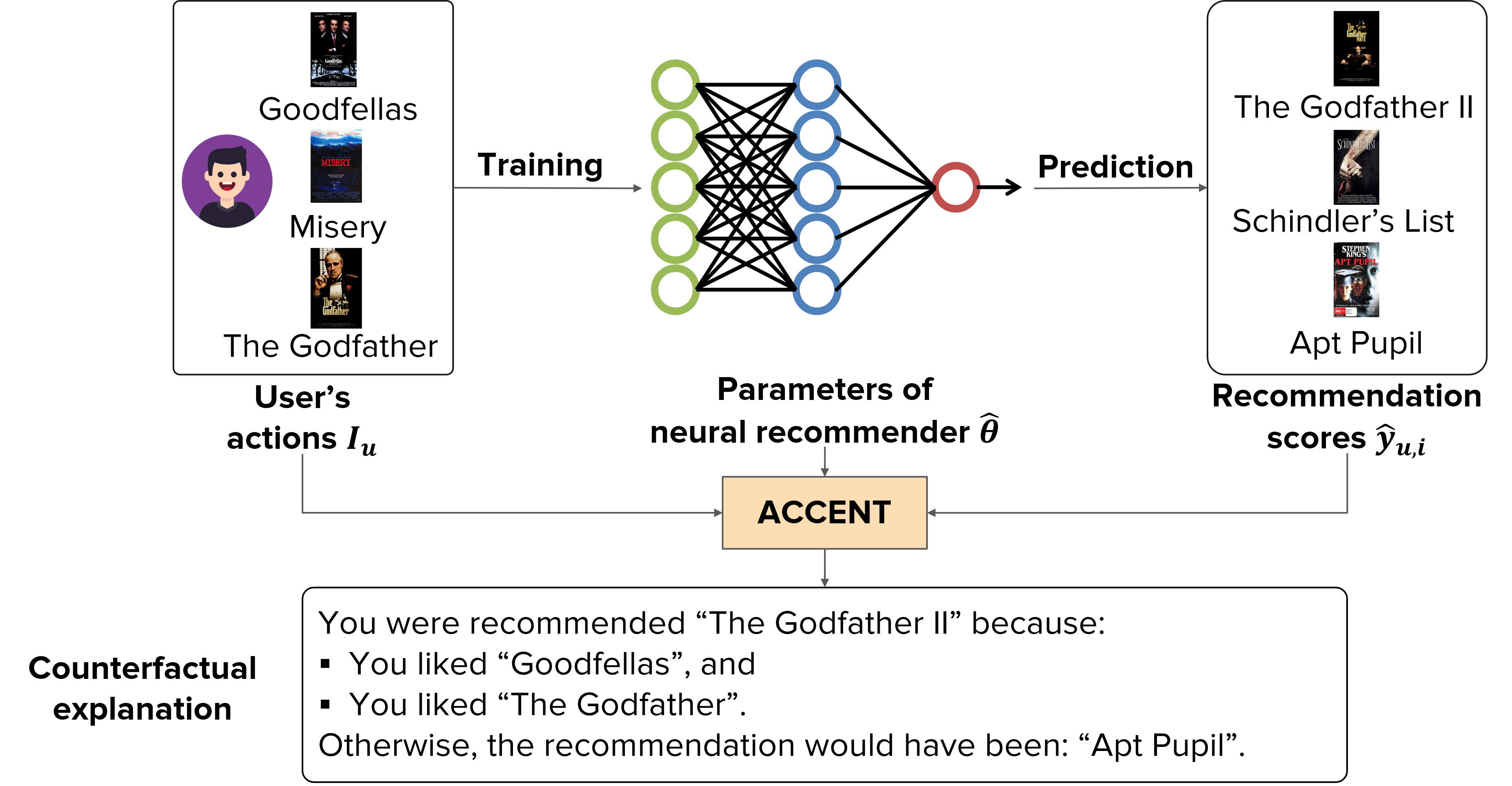
Figure 1. Positioning Accent in a neural recommender setup. Taking the user’s actions, parameters of the neural recommender, and predicted scores for items as input, Accent produces a concise counterfactual explanation.

Motivation. Recommender systems have become ubiquitous in today’s online world, spanning e-commerce to news to social media. It is fairly well-accepted that high-quality explanations (Ribeiro et al., 2016; Lundberg and Lee, 2017; Chen et al., 2018a) for the recommended content can help improve users’ satisfaction, while being actionable towards improving the underlying models (Ghazimatin et al., 2021; Balog and Radlinski, 2020; Lu et al., 2018b; Zhang and Chen, 2020; Zhao et al., 2019; Luo et al., 2020). Typical methods explaining neural recommenders face certain concerns: (i) they often rely on the attention mechanism to find important words (Seo et al., 2017), reviews (Chen et al., 2018b), or regions in images (Chen et al., 2019), which is still controversial (Jain and Wallace, 2019; Wiegreffe and Pinter, 2019); (ii) use connecting paths between users and items (Yang et al., 2018; Ai et al., 2018; Xian et al., 2019) that may not really be actionable and have privacy concerns; and, (iii) they use external item metadata such as reviews (Seo et al., 2017; Wu et al., 2019; Lu et al., 2018a) or images (Chen et al., 2019; Wu et al., 2019), that may not always be available.

In this context, it is reasonable to assume that in order to be tangible to end users, such explanations should relate to the user’s own activity, and be scrutable, actionable, and concise (Balog et al., 2019; Ghazimatin et al., 2019). This paved the way to posit counterfactual explanations based on the user’s own actions as a viable mechanism to address the tangibility concern (Ghazimatin et al., 2020; Karimi et al., 2021; Lucic et al., 2021; Mothilal et al., 2020; Martens and Provost, 2014). A counterfactual explanation is a set of the user’s own actions, that, when removed, produces a different recommendation (referred to as a replacement item in this text). In tandem with the huge body of work on explanations, recommender models themselves have continued to become increasingly complex. In recent years, neural recommender systems have become the de facto standard in the community, owing to their power of learning the sophisticated non-linear interplay between several factors (Zhang et al., 2019; He et al., 2017; Xin et al., 2019). However, this same complexity prevents us from generating counterfactual explanations with the same methodology that works well for graph-based recommenders (the Prince algorithm (Ghazimatin et al., 2020)).

Approach. To address this research gap, we present our method Accent (Action-based Counterfactual Explanations for Neural Recommenders for Tangibility), that extends the basic idea in Prince to neural recommenders. However, this necessitates tackling two basic challenges: (i) Prince relied on estimating contribution scores of a user’s actions using Personalized PageRank for deriving counterfactual sets, something that does not carry over to arbitrary neural recommenders; and (ii) the graph-based theoretical formalisms that form the core of the Prince algorithm, and ensure its optimality, also do not readily extend to deep learning models. To overcome these obstacles, we adapt the recently proposed Fast Influence Analysis (FIA) (Cheng et al., 2019) mechanism that sorts the user’s actions based on their approximate influence on the prediction from the neural recommender. While such influence scores are a viable proxy for the contribution scores above, they cannot be directly used to produce counterfactual sets. Accent extends the use of influence scores from single data points to pairs of items, the pair being the recommendation item and its replacement. This is a key step that enables producing counterfactual sets by iteratively closing the score gap between the original recommendation and a candidate replacement item from the original top-$k$ recommendations.

Figure 1 illustrates a typical counterfactual explanation output by Accent for the recommendation The Godfather II: had the user not watched movies Goodfellas and The Godfather, she would have been recommended Apt Pupil instead. More formally, given a user $u$, a list $I_{u}$ of items interacted by $u$ (her own actions), and a recommendation $rec$, Accent finds a counterfactual explanation $I_{u}^{*}\subseteq I_{u}$ whose removal from the training set results in a different recommendation $rec^{*}$. We apply Accent to explain predictions from two prominent neural recommenders, Neural Collaborative Filtering (NCF) (He et al., 2017) and Relational Collaborative Filtering (RCF) (Xin et al., 2019), and validate it on a subset of the MovieLens 100K dataset. All code and data are available at https://www.mpi-inf.mpg.de/impact/counterfactual-explanations-for-recommenders and https://github.com/hieptk/accent.

2. Method

2.1. Estimating parameters

Rooted in statistics, influence functions estimate how the model parameters change when a data point is upweighted by a small amount $\epsilon$ (Hampel, 1974). Using influence functions, Koh and Liang (Koh and Liang, 2017) proposed a method for estimating the impact of removing a data point from the training set (reducing its weight to $0$) on the model parameters. To briefly describe this method, let $\hat{\theta}$ be the original model parameters, i.e., $\hat{\theta}$ is the minimizer of the empirical risk:

(1) $$R(\theta)=\frac{1}{n}\sum_{i=1}^{n}L(z_{i},\theta)$$

where $n$ is the number of training points and $L(z_{i},\theta)$ is the loss of training point $z_{i}$ using parameters $\theta$. After upweighting training point $z$ by a small amount $\epsilon$, the new optimal parameters ($\hat{\theta}_{\epsilon,z}$) are approximated as follows:

(2) $$\hat{\theta}_{\epsilon,z}=\arg\min_{\theta\in\Theta}\{R(\theta)+\epsilon L(z,\theta)\}$$

According to (Koh and Liang, 2017), the influence of upweighting training point $z$ by a small amount $\epsilon$ is given by:

(3) $$\frac{d\hat{\theta}_{\epsilon,z}}{d\epsilon}\Big{|}_{\epsilon=0}=-H_{\hat{\theta}}^{-1}\nabla L(z,\hat{\theta})$$

where $H_{\hat{\theta}}$ is the Hessian matrix computed as $H_{\hat{\theta}}=\frac{1}{n}\sum_{i=1}^{n}\nabla_{\theta}^{2}L(z_{i},\hat{\theta})$. Since the weight of each training point is $\frac{1}{n}$, removing a training point $z$ is equivalent to upweighting it by $-\frac{1}{n}$. We can estimate the new parameters $\hat{\theta}^{-z}$ after removing $z$ by setting $\epsilon=-\frac{1}{n}$ in (3):

(4) $$\hat{\theta}^{-z}-\hat{\theta}=\frac{1}{n}H_{\hat{\theta}}^{-1}\nabla L(z,\hat{\theta})$$

Note that, since neural models are not convex, we enforce the invertibility of $H_{\hat{\theta}}$ by adding a small damping term $\lambda$ to its diagonal.

A challenge while applying influence functions to neural models is that the set of parameters is usually huge. FIA (Cheng et al., 2019) is a technique to reduce the computational cost of influence functions for recommender systems, and we will adapt this approach to our algorithm.

2.2. Computing influence on score gaps

Using FIA, we can estimate the new parameters $\hat{\theta}^{-z}$ when one training point (one of the user’s actions $I_{u}$) is removed. Substituting $\hat{\theta}^{-z}$ into the recommender model, we can estimate the new predicted score for any item. We denote the preference score of user $u$ for item $i$ before and after removing point $z$ as $\hat{y}_{u,i}$ and $\hat{y}_{u,i}^{-z}$, respectively. The influence of $z$ on $\hat{y}_{u,i}$ is defined as:

(5) $$I(z,\hat{y}_{u,i})=\hat{y}_{u,i}-\hat{y}_{u,i}^{-z}$$

We can then estimate the influence of a training point $z$ on the score gap between two items $i$ and $j$ as:

$$I(z,\hat{y}_{u,i}-\hat{y}_{u,j})=(\hat{y}_{u,i}-\hat{y}_{u,j})-(\hat{y}_{u,i}^{-z}-\hat{y}_{u,j}^{-z})$$

(6) $$=(\hat{y}_{u,i}-\hat{y}_{u,i}^{-z})-(\hat{y}_{u,j}-\hat{y}_{u,j}^{-z})=I(z,\hat{y}_{u,i})-I(z,\hat{y}_{u,j})$$

For a set of points $Z=\{z_{1},z_{2},...,z_{m}\}$, we approximate the influence of removing this set by:

(7) $$I(Z,\hat{y}_{u,i}-\hat{y}_{u,j})=\sum_{k=1}^{m}I(z_{k},\hat{y}_{u,i}-\hat{y}_{u,j})$$

With the increase in the size of the set $Z$, the accuracy of the above estimation deteriorates. However, since counterfactual sets are usually very small, this approximation is still valid.

2.3. Filling the gap

To replace the recommendation $rec$ with $rec^{*}$, we need to find a counterfactual explanation set $Z\subseteq I_{u}$ whose removal results in:

$$\hat{y}^{-Z}_{u,rec}-\hat{y}^{-Z}_{u,rec^{*}}<0$$

$$\Leftrightarrow\hat{y}_{u,rec}-\hat{y}_{u,rec^{*}}-\hat{y}^{-Z}_{u,rec}+\hat{y}^{-Z}_{u,rec^{*}}>\hat{y}_{u,rec}-\hat{y}_{u,rec^{*}}$$

$$\Leftrightarrow I(Z,\hat{y}_{u,rec}-\hat{y}_{u,rec^{*}})>\hat{y}_{u,rec}-\hat{y}_{u,rec^{*}}$$

(8) $$\Leftrightarrow\sum_{k=1}^{m}I(z_{k},\hat{y}_{u,rec}-\hat{y}_{u,rec^{*}})>\hat{y}_{u,rec}-\hat{y}_{u,rec^{*}}$$

Therefore, the optimal way to replace $rec$ with $rec^{*}$ is to add training points $z_{k}$ to $Z$ in the order of decreasing $I(z_{k},\hat{y}_{u,rec}-\hat{y}_{u,rec^{*}})$ until (8) is satisfied. To find the smallest counterfactual explanation $I_{u}^{*}$, we try every replacement item from a set of candidates $I_{rep}$. In principle, $I_{rep}$ could span the complete set of items $I$, but a practical choice is the original set of top-$k$ recommendations. Good models usually diversify their top-$k$ while preserving relevance, and choosing the replacement from this slate ensures that $rec^{*}$ is neither trivially similar to $rec$ nor irrelevant to $u$. Finally, this smallest set of actions $I_{u}^{*}$ is returned to $u$ as a tangible explanation for $rec$. Algorithm 1 contains a precise formulation of Accent. Accent’s time complexity is $O(|I_{rep}|\times|I_{u}|\times\log|I_{u}|)$ + $O(|I_{rep}|\times|I_{u}|)$ calls of FIA. Since Accent only requires access to gradients and the Hessian matrix, it is applicable to a large class of neural recommenders.

Input: user $u$, recommendation item $rec$,

items interacted with by user $I_{u}$, candidate replacement items $I_{rep}$

Output: smallest counterfactual set $I_{u}^{*}$, replacement $rec^{*}$

$I_{u}^{*},rec^{*}\leftarrow I_{u},-1$

for $i\in I_{rep}$ do

       for $z\in I_{u}$ do // Compute influence on gap

             compute $I(z,\hat{y}_{u,rec})$ and $I(z,\hat{y}_{u,i})$

             $I(z,\hat{y}_{u,rec}-\hat{y}_{u,i})\leftarrow I(z,\hat{y}_{u,rec})-I(z,\hat{y}_{u,i})$

            

       end for

      $gap,I_{u}^{i}\leftarrow\hat{y}_{u,rec}-\hat{y}_{u,i},\emptyset$

       sort $I_{u}$ by decreasing $I(z,\hat{y}_{u,rec}-\hat{y}_{u,i})$

       for $z\in sorted(I_{u})$ do

             if $gap<0$ or $I(z,\hat{y}_{u,rec}-\hat{y}_{u,i})\leq 0$ then

                  

                   // Gap is filled or impossible

                   break

                  

             end if

            $gap\leftarrow gap-I(z,\hat{y}_{u,rec}-\hat{y}_{u,i})$

              // Update gap

             $I_{u}^{i}\leftarrow I_{u}^{i}\cup\{z\}$

              // and result set

            

       end for

      if $gap<0$ and $|I_{u}^{i}|<|I_{u}^{*}|$ then // New smallest set

             $I_{u}^{*},rec^{*}\leftarrow I_{u}^{i},i$

            

       end if

      

end for

return $I_{u}^{*},rec^{*}$

Algorithm 1 Accent

3. Experimental Setup

3.1. Recommender models

We apply Accent on NCF (He et al., 2017), one of the first neural recommenders, and RCF (Xin et al., 2019), a more recent choice. NCF (He et al., 2017) consists of a generalized matrix factorization layer (where the user and the item embeddings are element-wise multiplied), and a multilayer perceptron that takes these user and item embeddings as input. These two parts are then combined to predict the final recommendation score. RCF uses auxiliary information to incorporate item-item relations into the model. It computes target-aware embeddings that capture information about the user, her interactions, and their relationships with target items (recommendation candidates) using a two-layer attention scheme. The recommendation score of the user and the target item are computed from these target-aware embeddings.

3.2. Dataset

We use the popular MovieLens $100$K dataset (Harper and Konstan, 2015), which contains $100k$ ratings on a $1-5$ scale by $943$ users on $1682$ movies. Input of this form can be directly fed into NCF. On the other hand, to conform to the implicit feedback setting in RCF, we binarized ratings to a positive label if it is $3$ or above, and a negative label otherwise. We removed all users with $<\!10$ positive ratings or $<\!10$ negative ratings so that the profiles are big and balanced enough for learning discriminative user models. This pruning results in $452$ users, $1654$ movies, and $61054$ interactions in our dataset. For item-item relations in RCF, we used the auxiliary data provided in (Xin et al., 2019), which contains four relation types and $97209$ relation pairs.

3.3. Baselines

We compare Accent against four baseline algorithms. Two baselines are based on the attention weights in RCF and are not applicable to NCF, while the other two algorithms are based on FIA scores and can be used for both recommender models.

3.3.1. Attention-based algorithms

Attention weights in RCF can be used to produce explanations (Xin et al., 2019). An item’s attention weight shows how much it affects the prediction: thus, to find a counterfactual explanation for $rec$, we can sort all items in $I_{u}$ by decreasing attention weights. We then add these items one by one to $I_{u}^{*}$ until the predicted recommendation is changed. Here, we assume removing a few training points does not change the model significantly, so all parameters remain fixed. We refer to this as pure attention. We adapt pure attention to a smarter attention baseline, where an item is added to $I_{u}^{*}$ only if removing it reduces the score gap between $\hat{y}_{u,rec}$ and the second-ranked item’s score. The underlying intuition is to avoid adding potentially irrelevant items to the explanation. The score gap is again estimated using fixed parameters.

3.3.2. FIA-based algorithms

Here, we test the direct applicability of FIA to produce counterfactual explanations. We simply sort items in $I_{u}$ by $I(z,\hat{y}_{u,rec})$ and add items one by one to $I_{u}^{*}$ until $rec$ is displaced (pure FIA). As with attention, we improve pure FIA to keep only the interactions that reduce the score gap between $\hat{y}_{u,rec}$ and the score of the second-ranked item (strategy denoted by FIA).

3.4. Initialization

For FIA on NCF, we used the implementation in (Cheng et al., 2019). We used a batch size $1246$ as this implementation requires this value to be a factor of the dataset size ($61054$). All other hyperparameters were kept the same. For RCF, we set the dropout rate to $0$ to minimize randomness during retraining. We replaced the ReLU activation with GELU (Hendrycks and Gimpel, 2020) to avoid problems with non-differentiability (Koh and Liang, 2017). To guarantee FIA’s effectiveness, we made sure that each interaction corresponds to one training point (that was fifty in the original model). For this, we paired each liked item $i^{+}$ by user $u$ with one of her disliked items $i^{-}$, and added triples $(u,i^{+},i^{-})$ to the training set. In particular, for each $i^{+}$, we selected an $i^{-}$ that shares the highest number of relations with $i^{+}$. By doing this principled negative sampling, the RCF model can still discriminate between positive and negative items effectively, despite having only one negative item for each positive. For FIA on RCF, we added damping term $\lambda=0.01$ to the Hessian matrix and used our own implementation.

4. Results and insights

4.1. Evaluation protocol

For each of the $452$ users in our dataset, we find an explanation $I_{u}^{*}$ for their recommendation $rec$, and a replacement $rec^{*}$ from $I_{rep}$, where $I_{rep}$ is the original top-$k$ ($k=5,10,20$). We then retrain the models without $I_{u}^{*}$ and verify if $rec^{*}$ replaces $rec$. This is done for both recommender models (NCF and RCF) and each of the explanation algorithms (Accent, pure attention, attention, pure FIA and FIA, as applicable). The percentages of actual replacements (CF percentage) and the average sizes of the counterfactual sets (CF set size) for Accent and the baselines are reported in Table 1. Ideally, an algorithm should have a high CF percentage and a small CF set size. To give a qualitative feel of the explanations generated by Accent, we provide some anecdotal examples in Table 2 (baselines had larger CF sets). To compare the counterfactual effect (CF percentages) between two methods, we used the McNemar’s test for paired binomial data, since each explanation is either actually counterfactual or not (binary). For CF set sizes, we used the one-sided paired $t$-test. The significance level for all tests was set to $0.05$.

Candidate top-k set of replacement items		$k=5$		$k=10$		$k=20$
Recommender model	Explanation model	CF percentage	CF set size	CF percentage	CF set size	CF percentage	CF set size
NCF (He et al., 2017)	Pure FIA (Cheng et al., 2019)	$54.20$	$9.08$	$56.19$	$9.46$	$55.75$	$9.50$
	FIA (Cheng et al., 2019)	$55.97$	$7.98$	$56.19$	$7.80$	$55.75$	$7.84$
	ACCENT (Proposed)	$\boldsymbol{57.30}$	$\boldsymbol{4.73^{*}}$	$\boldsymbol{57.74}$	$\boldsymbol{4.69^{*}}$	$\boldsymbol{57.08}$	$\boldsymbol{4.62^{*}}$
RCF (Xin et al., 2019)	Pure Attention (Xin et al., 2019)	$73.01$	$9.36$	$73.45$	$7.94$	$74.34$	$7.75$
	Attention (Xin et al., 2019)	$76.99$	$3.55$	$76.99$	$3.53$	$76.99$	$3.51$
	Pure FIA (Cheng et al., 2019)	$80.75$	$4.85$	$81.19$	$4.62$	$81.86$	$4.72$
	FIA (Cheng et al., 2019)	$81.64$	$4.15$	$81.86$	$4.10$	$81.86$	$4.10$
	ACCENT (Proposed)	$\boldsymbol{81.86^{\dagger}}$	$\boldsymbol{2.83^{*\dagger}}$	$\boldsymbol{82.08^{\dagger}}$	$\boldsymbol{2.75^{*\dagger}}$	$\boldsymbol{82.08^{\dagger}}$	$\boldsymbol{2.74^{*\dagger}}$

Best values in each column are in bold. * and ^† denote statistical significance of Accent over FIA and Attention, respectively.

Table 1. Performance comparison of Accent with baselines on our sample of the MovieLens 100K benchmark.

Recommendation	Accent Explanation	Replacement
The Silence Of The Lambs	Contact Fargo	Donnie Brasco
Titanic	True Romance The Basketball Diaries	East Of Eden
The Devil’s Advocate	Speed Eraser It’s A Wonderful Life	My Fair Lady

Table 2. Counterfactual sets generated by Accent.

4.2. Key findings

Accent is effective. For both models, Accent produced the best overall results for producing counterfactual explanations. Results are statistically significant for CF percentages over attention baselines, and for CF set sizes over both attention and FIA methods (marked with asterisks and daggers in Table 1).

Attention is not explanation. The two algorithms using attention performed the worst. Their CF percentage is at least $5\%$ lower than Accent and their average CF set sizes are between $1.3$ to $3.3$ times bigger than Accent. This shows that using attention is not really helpful in finding concise counterfactual explanations.

FIA is not enough. The two algorithms that directly use FIA to rank interactions produced very big explanations. The average size of FIA’s explanations is $1.5$ to $1.7$ times bigger than that of Accent (about twice as big for pure FIA with NCF, the context in which FIA was originally proposed). This provides evidence that to replace $rec$, the influence on the score gap is more important than the influence on the score of $rec$ alone.

Considering the score gap is essential. The two pure algorithms that do not consider the score gap between $rec$ and the replacement while expanding the explanation, performed worse than their smarter versions that do take this gap reduction into account. The difference can be as large as $4\%$ in CF percentages, with up to $2.6$ times bigger CF sets (pure attention, $k=5$).

Influence estimation for sets is adequate. Our approximation of FIA for sets of items is actually quite close to the true influence. For RCF, the RMSE between the approximated influence and the true influence is $1.17$ over different values of $k$, which is small compared to the standard deviation of the true influence ($\simeq 3.7$). For NCF, this RMSE is $0.36$ while the true influence has a standard deviation of $0.34$, implying that estimation accuracy is lower for this model: this in turn results in a lower CF percentage.

Explanations get smaller as $k$ grows. The performance of Accent is stable across different $k\;(5,10,20)$, varying less than $1\%$. The average CF set size slightly decreases as $k$ increases, because we have more options to replace $rec$ with. Interestingly, a similar effect was observed in the graph-based setup in Prince (Ghazimatin et al., 2020).

4.3. Analysis

Pairwise vis-à-vis one-versus-all. In our main algorithm, instead of fixing one replacement item at a time (pairwise), we can have a different approach that does not need a fixed replacement. In particular, at each step, we can reduce the gap between $rec$ and the second-ranked item at the time, leaving this second-ranked item to change freely during the process (one-versus-all). Through experiments, we found that this approach can slightly improve the counterfactual percentage of Accent by $0.22\%$ on RCF but at the cost of bigger explanations.

Error analysis. Despite being effective in estimating influence, FIA is still an approximation. In particular, it assumes that only a few parameters are affected by the removal of a data point (corresponding user and item embeddings). This assumption can sometimes lead to errors in practice. In NCF, we observed a large discrepancy between the estimated influence and the actual score drops, despite their strong correlation ($\rho=0.77$). This explains Accent’s relatively low CF percentages in NCF ($\simeq 57\%$). It would thus be desirable to update more parameters when one action is removed: for example, in RCF, we can also consider relation type and relation value embeddings. However, this could substantially increase the computational cost. Another source of error is that the influence of a set of items is sometimes overestimated. This can cause Accent to stop prematurely when the cumulative influence is not enough to swap two items. To mitigate this, we can retrain the model after Accent stops, to verify whether the result is actually counterfactual. If not, Accent can resume and add more actions.

5. Conclusion

We described Accent, a mechanism for generating counterfactual explanations for neural recommenders. Accent extends ideas from the Prince algorithm to the neural setup, while using and adapting influence values from FIA for the pairwise contribution scores that were a core component of Prince but non-trivial to obtain in deep models. We demonstrated Accent’s effectiveness over attention and FIA baselines with the underlying recommender being NCF or RCF, but it is applicable to a much broader class of models: the only requirements are access to gradients and the Hessian.

Acknowledgements. This work was supported by the ERC Synergy Grant 610150 (imPACT).

References

- (1)
- Ai et al. (2018) Qingyao Ai, Vahid Azizi, Xu Chen, and Yongfeng Zhang. 2018. Learning heterogeneous knowledge base embeddings for explainable recommendation. Algorithms 11, 9 (2018).
- Balog and Radlinski (2020) Krisztian Balog and Filip Radlinski. 2020. Measuring Recommendation Explanation Quality: The Conflicting Goals of Explanations. In SIGIR.
- Balog et al. (2019) Krisztian Balog, Filip Radlinski, and Shushan Arakelyan. 2019. Transparent, scrutable and explainable user models for personalized recommendation. In SIGIR.
- Chen et al. (2018b) Chong Chen, Min Zhang, Yiqun Liu, and Shaoping Ma. 2018b. Neural attentional rating regression with review-level explanations. In WWW.
- Chen et al. (2018a) Jianbo Chen, Le Song, Martin Wainwright, and Michael Jordan. 2018a. Learning to explain: An information-theoretic perspective on model interpretation. In ICML.
- Chen et al. (2019) Xu Chen, Hanxiong Chen, Hongteng Xu, Yongfeng Zhang, Yixin Cao, Zheng Qin, and Hongyuan Zha. 2019. Personalized Fashion Recommendation with Visual Explanations Based on Multimodal Attention Network: Towards Visually Explainable Recommendation. In SIGIR.
- Cheng et al. (2019) Weiyu Cheng, Yanyan Shen, Linpeng Huang, and Yanmin Zhu. 2019. Incorporating Interpretability into Latent Factor Models via Fast Influence Analysis. In KDD.
- Ghazimatin et al. (2020) Azin Ghazimatin, Oana Balalau, Rishiraj Saha Roy, and Gerhard Weikum. 2020. PRINCE: Provider-Side Interpretability with Counterfactual Explanations in Recommender Systems. In WSDM.
- Ghazimatin et al. (2021) Azin Ghazimatin, Soumajit Pramanik, Rishiraj Saha Roy, and Gerhard Weikum. 2021. ELIXIR: Learning from User Feedback on Explanations to Improve Recommender Models. arXiv:cs.IR/2102.09388
- Ghazimatin et al. (2019) Azin Ghazimatin, Rishiraj Saha Roy, and Gerhard Weikum. 2019. FAIRY: A Framework for Understanding Relationships between Users’ Actions and their Social Feeds. In WSDM.
- Hampel (1974) Frank R. Hampel. 1974. The Influence Curve and Its Role in Robust Estimation. J. Amer. Statist. Assoc. (1974).
- Harper and Konstan (2015) F. Maxwell Harper and Joseph A. Konstan. 2015. The MovieLens Datasets: History and Context. TiiS (2015).
- He et al. (2017) Xiangnan He, Lizi Liao, Hanwang Zhang, Liqiang Nie, Xia Hu, and Tat-Seng Chua. 2017. Neural Collaborative Filtering. In WWW.
- Hendrycks and Gimpel (2020) Dan Hendrycks and Kevin Gimpel. 2020. Gaussian Error Linear Units (GELUs). arXiv:cs.LG/1606.08415
- Jain and Wallace (2019) Sarthak Jain and Byron C. Wallace. 2019. Attention is not Explanation. In NAACL.
- Karimi et al. (2021) Amir-Hossein Karimi, Bernhard Schölkopf, and Isabel Valera. 2021. Algorithmic recourse: From counterfactual explanations to interventions. In FACCT.
- Koh and Liang (2017) Pang Wei Koh and Percy Liang. 2017. Understanding Black-box Predictions via Influence Functions. In ICML.
- Lu et al. (2018a) Yichao Lu, Ruihai Dong, and Barry Smyth. 2018a. Coevolutionary Recommendation Model: Mutual Learning between Ratings and Reviews. In WWW.
- Lu et al. (2018b) Yichao Lu, Ruihai Dong, and Barry Smyth. 2018b. Why I like it: Multi-task learning for recommendation and explanation. In RecSys.
- Lucic et al. (2021) Ana Lucic, Maartje ter Hoeve, Gabriele Tolomei, Maarten de Rijke, and Fabrizio Silvestri. 2021. CF-GNNExplainer: Counterfactual Explanations for Graph Neural Networks. arXiv:cs.LG/2102.03322
- Lundberg and Lee (2017) Scott M Lundberg and Su-In Lee. 2017. A Unified Approach to Interpreting Model Predictions. In NIPS.
- Luo et al. (2020) Kai Luo, Hojin Yang, Ga Wu, and Scott Sanner. 2020. Deep Critiquing for VAE-Based Recommender Systems. In SIGIR.
- Martens and Provost (2014) David Martens and Foster Provost. 2014. Explaining data-driven document classifications. MIS Quarterly 38, 1 (2014).
- Mothilal et al. (2020) Ramaravind K Mothilal, Amit Sharma, and Chenhao Tan. 2020. Explaining machine learning classifiers through diverse counterfactual explanations. In FACCT.
- Ribeiro et al. (2016) Marco Tulio Ribeiro, Sameer Singh, and Carlos Guestrin. 2016. “Why should I trust you?” Explaining the predictions of any classifier. In KDD.
- Seo et al. (2017) Sungyong Seo, Jing Huang, Hao Yang, and Yan Liu. 2017. Interpretable Convolutional Neural Networks with Dual Local and Global Attention for Review Rating Prediction. In RecSys.
- Wiegreffe and Pinter (2019) Sarah Wiegreffe and Yuval Pinter. 2019. Attention is not not Explanation. In EMNLP-IJCNLP.
- Wu et al. (2019) Libing Wu, Cong Quan, Chenliang Li, Qian Wang, Bolong Zheng, and Xiangyang Luo. 2019. A Context-Aware User-Item Representation Learning for Item Recommendation. TOIS (2019).
- Xian et al. (2019) Yikun Xian, Zuohui Fu, S Muthukrishnan, Gerard De Melo, and Yongfeng Zhang. 2019. Reinforcement knowledge graph reasoning for explainable recommendation. In SIGIR.
- Xin et al. (2019) Xin Xin, Xiangnan He, Yongfeng Zhang, Yongdong Zhang, and Joemon Jose. 2019. Relational Collaborative Filtering: Modeling Multiple Item Relations for Recommendation. In SIGIR.
- Yang et al. (2018) Fan Yang, Ninghao Liu, Suhang Wang, and Xia Hu. 2018. Towards interpretation of recommender systems with sorted explanation paths. In ICDM.
- Zhang et al. (2019) Shuai Zhang, Lina Yao, Aixin Sun, and Yi Tay. 2019. Deep Learning Based Recommender System: A Survey and New Perspectives. ACM Comput. Surv. (2019).
- Zhang and Chen (2020) Yongfeng Zhang and Xu Chen. 2020. Explainable Recommendation: A Survey and New Perspectives. Foundations and Trends® in Information Retrieval (2020).
- Zhao et al. (2019) Guoshuai Zhao, Hao Fu, Ruihua Song, Tetsuya Sakai, Zhongxia Chen, Xing Xie, and Xueming Qian. 2019. Personalized reason generation for explainable song recommendation. TIST 10, 4 (2019).