Prominent characteristics of recurrent neuronal networks are robust against low synaptic weight resolution

Abstract

The representation of the natural-density, heterogeneous connectivity of neuronal network models at relevant spatial scales remains a challenge for Computational Neuroscience and Neuromorphic Computing. In particular, the memory demands imposed by the vast number of synapses in brain-scale network simulations constitutes a major obstacle. Limiting the number resolution of synaptic weights appears to be a natural strategy to reduce memory and compute load. In this study, we investigate the effects of a limited synaptic-weight resolution on the dynamics of recurrent spiking neuronal networks resembling local cortical circuits, and develop strategies for minimizing deviations from the dynamics of networks with high-resolution synaptic weights. We mimic the effect of a limited synaptic weight resolution by replacing normally distributed synaptic weights by weights drawn from a discrete distribution, and compare the resulting statistics characterizing firing rates, spike-train irregularity, and correlation coefficients with the reference solution. We show that a naive discretization of synaptic weights generally leads to a distortion of the spike-train statistics. Only if the weights are discretized such that the mean and the variance of the total synaptic input currents are preserved, the firing statistics remains unaffected for the types of networks considered in this study. For networks with sufficiently heterogeneous in-degrees, the firing statistics can be preserved even if all synaptic weights are replaced by the mean of the weight distribution. We conclude that even for simple networks with non-plastic neurons and synapses, a discretization of synaptic weights can lead to substantial deviations in the firing statistics, unless the discretization is performed with care and guided by a rigorous validation process. For the network model used in this study, the synaptic weights can be replaced by low-resolution weights without affecting its macroscopic dynamical characteristics, thereby saving substantial amounts of memory.

Keywords: neuromorphic computing, spiking neuronal network, network heterogeneity, synaptic-weight discretization, validation, activity statistics

1 Introduction

Computational neuronal network models constrained by available biological data constitute a valuable tool for studying brain function. The large number of neurons in the brain, their dense connectivity, and the premise that advanced brain functions involve a complex interplay of different brain regions (Bressler and Menon, 2010) pose high computational demands on model simulations. The human cortex consists of more than $10^{10}$ neurons (Herculano-Houzel, 2009), each receiving about $10^{4}$ connections (Abeles, 1991; DeFelipe et al., 2002). The requirements for simulations of networks at this scale by far exceed the limits of modern workstations. Even on high-performance computing (HPC) systems that distribute the work load across many compute nodes running designated simulation software, neuronal networks larger than 10% of the human cortex are not accessible to simulation to date (Jordan et al., 2018). Studying downscaled networks with reduced neuron and synapse numbers does not qualify as an alternative to natural-density full-scale networks: while parameter adjustments can compensate to preserve some characteristics of the network dynamics such as firing rates, or the sensitivity to small perturbations (Bachmann et al., 2020), other features such as the structure of pairwise correlations in the neuronal activity cannot be maintained simultaneously (van Albada et al., 2015).

The complexity of neuronal network models evaluated on conventional HPC systems is limited by simulation speed and hardware requirements. Routine simulations of large-scale natural-density networks are still not a standard. Even with state-of-the-art software and high-performance machines, simulations of biological processes may take several hundred times longer than the respective processes in the brain (Jordan et al., 2018). Biological processes evolving on long time scales (hours, days, up to years) such as learning and brain development are therefore impossible to simulate in reasonable amounts of time. In addition, the power consumption of large-scale network simulations on HPC systems exceeds the demands of biological brains by orders of magnitude (van Albada et al., 2018). In this study, we address another factor obstructing large-scale neuronal network simulations: the high memory demand (Kunkel et al., 2012, 2014). In simulations performed with NEST (Gewaltig and Diesmann, 2007), a simulation software optimized for this application area, the required memory is mainly used for the storage of synapses (Jordan et al., 2018). While the network model by Jordan et al. (2018) involves dynamic synapses undergoing spike-time dependent plasticity, the problem persists also for the simplest static synapse models characterized by a constant weight and transmission delay. Using double-precision floating point numbers, NEST requires $64$ bit of memory for the weight and $24$ bit for the delay of each synapse (Kunkel et al., 2014). In the mammalian neocortex, the number of synapses exceeds the number of neurons by a factor of $10^{4}$. Hence, even small memory demands for individual synapses add up to substantial amounts in brain-scale simulations. Reduced memory consumption leads to faster simulation because the network model can be represented on fewer compute nodes, thereby reducing the time required for communication between nodes. Access patterns of synapses are highly variable due to the random structure of neuronal networks and their sparse and irregular activity. Therefore, also on the individual compute nodes a reduced memory consumption helps as memory access can better be predicted and more of the required memory fits into the cache.

While these and other limitations may not be overcome using conventional computers built upon the von-Neumann architecture (Backus, 1978; Indiveri and Liu, 2015), the development of novel, brain-inspired hardware architectures promises a solution. Examples for these so-called neuromorphic hardware systems with different levels of maturity are SpiNNaker (Furber et al., 2013), BrainScaleS (Meier, 2015), Loihi (Davies et al., 2018), TrueNorth (Merolla et al., 2014), and Tianjic (Pei et al., 2019). All of these systems are designed after different principles and with different aims (Furber, 2016), and they employ different strategies for handling synaptic weights in an architecture with typically little available memory. SpiNNaker, for instance, saves the weights as $16$-bit integer values (Jin et al., 2009) and uses fixed-point arithmetic for the computations. BrainScaleS, instead, utilizes a mixed signal approach where the dynamics of individual neurons are implemented by analog circuits embedded in a silicon wafer and the weight of each synapse is stored using only $6$-bit (Wunderlich et al., 2019). Similarly, GPUs (Knight and Nowotny, 2018; Golosio et al., 2021) and FPGAs (Gupta et al., 2015) are used for simulations of neural networks with reduced numerical precision.

Simulation results obtained with different (neuromorphic) hardware and software systems are hard to compare (Senk et al., 2017; Gutzen et al., 2018; van Albada et al., 2018). A number of inherent structural differences (e.g., numerical solvers) may obscure the role of reduced numerical precision on the network dynamics. Here, we systematically study the effects of a limited synaptic-weight resolution in software-based simulations of recurrently connected spiking neuronal networks. We mimic a limited synaptic-weight resolution by drawing synaptic weights from a discrete distribution with a predefined discretization level. All other parameters and dynamical variables are represented in double precision and all calculations are carried out using standard double arithmetic in the programming language C++. An exception are the spike times of the neurons which are bound to the time grid spanned by the computation time step $h$. This artificially increases synchronization in the network and introduces a global synchronization error of first order (Hansel et al., 1998; Morrison et al., 2007). The limitation can be overcome by treating spikes in continuous time. This is more costly if only a moderate precision is required but leads to shorter run times of high-precision simulations (Hanuschkin et al., 2010). However, in the models considered here the errors are dominated by other factors (van Albada et al., 2018). Frameworks like NEST may support both simulation strategies enabling the validation of grid-constrained results by continuous time simulations with minimal changes to the executable model description.

In the field of machine learning, a number of previous studies addresses the effects of low-resolution weights in artificial neural networks (e.g., Dundar and Rose, 1995; Draghici, 2002; Courbariaux et al., 2014; Gupta et al., 2015; Muller and Indiveri, 2015; Wu et al., 2016; Guo, 2018). These studies, however, do not provide any intuitive or theoretical explanation why a particular weight resolution is sufficient to achieve a desirable network performance. It is therefore unclear to what extent the results of these studies generalize to other tasks or networks. It is particularly difficult to transfer these results to neuroscientific network models: while in machine learning networks are typically validated based on the achieved task performance, neuroscience often also focuses on the idle (“resting state”) or task related network activity. In this work, we address the origin of potential deviations in the dynamics of neuronal networks with reduced synaptic-weight resolution from those obtained with a high-resolution “reference” of the same network, and develop strategies to minimize these deviations. For some machine learning algorithms such as reservoir computing, the two views on performance are related as the functional performance depends on the dynamical characteristics of the underlying neuronal network. In general, however, task performance is not a predictor of network dynamics (and vice versa).

We demonstrate our general approach based on variants of the local cortical microcircuit model by Potjans and Diesmann (2014), the “PD model”. This model represents the cortical natural-density circuitry underneath a $1\,\mathrm{mm^{2}}$ patch of early sensory cortex with almost $80,000$ neurons and $\sim 10^{4}$ synapses per neuron, and explains the cell-type and cortical-layer specific firing statistics observed in nature. To account for the natural heterogeneity in connection strengths, the synaptic weights are normally distributed. The PD model may serve as a building block for brain-size networks, because the fundamental characteristics of the cortical circuitry at this spatial scale are similar across different cortical areas and species. In the recent past, the PD model served as a benchmark for several validation studies in the rapidly evolving field of Neuromorphic Computing (van Albada et al., 2018; Knight and Nowotny, 2018; Rhodes et al., 2019; Heittmann et al., 2020; Kurth et al., 2020; Golosio et al., 2021). With this manuscript, we aim to add the aspect of weight discretization to the debate.

The manuscript is organized as follows: Section 2 provides details on the discretization methods, the validation procedure, the network model, and the network simulations. Section 3.1 exposes the pitfalls of a naive discretization of synaptic weights and section 3.2 proposes an optimal discretization strategy for the given synaptic-weight distribution. For illustration, sections 3.1 and 3.2 are based on a variant of the PD model with fixed in-degrees, i.e., a network where each neuron within a population receives exactly the same number of inputs. In section 3.3, in contrast, the in-degrees are distributed (as in the original PD model), allowing for a generalization of the results. Section 3.4 proposes an analytical approach using mean-field theory to substantiate the simulation results on the role of synaptic-weight and in-degree distributions. Section 3.5 investigates the effect of the simulation duration on the relevance of the employed validation metrics, and on the validation performance. The final section 4 summarizes the results and discusses future work towards precise and efficient neuronal network simulations.

2 Methods

The general approach of this study is to compare simulations of neuronal networks with differently discretized synaptic weights. To assess whether the weight discretization influences the network dynamics, the statistics of the spiking activity in the networks with discretized weights are compared with the statistics in the reference network with double precision weights. The following sections describe the methods used for discretizing the synaptic weights (section 2.1) and for calculating and comparing the network statistics (section 2.2). Section 2.3 contains specifications of the neuronal network models employed.

2.1 Discretization of synaptic weights

Computer number formats determine how many binary digits, i.e., bits, of computer memory are occupied by a numerical value and how these bits are interpreted (Goldberg, 1991). Both the number of bits, $N_{\text{bits}}$, and their interpretation differ for the various floating-point and fixed-point formats deployed in software and hardware. A common format is the IEEE 754 double-precision binary floating-point format (binary64) which allocates $64$ bits of memory per value encoding the sign ($1$ bit), the exponent ($11$ bits), and the significant precision ($52$ bits). In general, the upper limit of distinguishable values that a format can represent is $2^{N_{\text{bits}}}$. We here aim to identify a possible lower limit for a bit resolution required to store the synaptic weights in neuronal network simulations without compromising the accuracy of the results. The network models studied in this work assume weights to be sampled from continuous distributions, yielding values in double precision in the respective reference implementations.

To mimic a lower bit resolution, we discretize the distributions and systematically reduce the number of attainable values. On the machine, the values are still represented in double precision, but the degrees of discretization considered are by orders of magnitude coarser than double precision. Our approach is therefore independent of the underlying number format. For generality and for explicit distinction from the format-specific $N_{\text{bits}}$, we define the weight resolution by the number of possible discrete values, $N_{\text{bins}}$, that a discrete distribution is composed of. In the studied network models, projections between different pairs of neuronal populations are parameterized with weights sampled from $N_{\text{distr}}$ distributions, for details see section 2.3. A weight resolution of $N_{\text{bins}}$ means that $N_{\text{bins}}$ weight values are assumed for each of the underlying distributions. The maximum total number of different weights in a network model with discretized weights is therefore $N_{\text{bins}}\cdot N_{\text{distr}}$ in addition to potentially different weights not sampled from a distribution, e.g., those used to connect external stimulating devices.

After the reference weight values are sampled from the continuous reference distribution, each one of these sampled weights is subsequently replaced by one of the $N_{\text{bins}}$ discrete values which are computed according to a discretization procedure as follows: first an interval $\left[w_{\text{min}},\,w_{\text{max}}\right]$ is defined. Then the interval is divided up into $N_{\text{bins}}$ bins of equal widths such that the left edge of the first bin is $w_{\text{min}}$ and the right edge of the last bin is $w_{\text{max}}$. For each bin, indexed by $i\in\text{$\left[1,\,...,\,N_{\text{bins}}\right]$}$, the center value $v_{i}$ is assumed as the discrete value for that bin:

$$v_{i}=w_{\text{min}}+\left(\frac{1}{2}+i-1\right)\cdot w_{\text{step}}\quad\text{with}\quad w_{\text{step}}=\frac{w_{\text{max}}-w_{\text{min}}}{N_{\text{bins}}}.$$ (1)

All weights drawn from the continuous reference distribution falling into a specific bin are replaced by the respective $v_{i}$, meaning that they are rounded to the nearest discrete value. If a sampled weight coincides with a bin edge, the larger one of the two possible $v_{i}$ is chosen. However, the probability that a double precision weight drawn from a distribution with a continuous probability density function falls exactly onto the edge of one discrete bin is almost zero. Weights outside of the interval $\left[w_{\text{min}},\,w_{\text{max}}\right]$ are rounded to the closest discrete values, namely the values of the first or last bin. The two discretization schemes used in this study (“naive” and “optimized”) differ in their choice of the boundaries of the interval.

2.1.1 Naive discretization of normal weight distribution

Without deeper considerations, it seems reasonable to choose $[w_{\text{min}},\,w_{\text{max}}]$ such that the number of originally drawn weights outside of this interval is negligible. As we are studying network models in which the underlying continuous weight distributions are normal distributions with mean $\overline{w}_{\infty}$ and standard deviation $\Delta w_{\text{$\infty$}}$, a choice could be:

$$\left[w_{\text{min}},\,w_{\text{max}}\right]=\left[\overline{w}_{\infty}-5\Delta w_{\text{$\infty$}},\,\overline{w}_{\infty}+5\Delta w_{\text{$\infty$}}\right].$$ (2)

2.1.2 Optimized discretization of normal weight distribution

An optimized choice for the boundaries of the interval takes statistical properties of the discrete weights into account. If the reference weights are independently generated according to a probability distribution $p(w)$, the distribution of the discrete weights is a probability mass function $p^{*}\left(v_{i}\right)=:p_{i}^{*}$ with

$$p_{i}^{*}=\left\{\begin{array}[]{lcl}F\left(w_{\text{min}}+w_{\text{step}}\right)-F\left(-\infty\right)&\text{if}&i=1\\ F\left(w_{\text{min}}+iw_{\text{step}}\right)-F\left(w_{\text{min}}+\left(i-1\right)w_{\text{step}}\right)&\text{if}&i=2,\dots,\left(N_{\text{bins}}-1\right)\\ F\left(\infty\right)-F\left(w_{\text{min}}+\left(N_{\text{bins}}-1\right)w_{\text{step}}\right)&\text{if}&i=N_{\text{bins}}\end{array}\right.$$ (3)

and $F(w)=\int_{-\infty}^{w}p\left(w^{\prime}\right)\,\text{d}w^{\prime}$. The statistical properties of the discrete weights are calculated as for any other discrete random variable; mean and standard deviation of the discrete weights are:

$$\overline{w}_{N_{\text{bins}}} = \sum_{i=1}^{N_{\text{bins}}}v_{i}p_{i}^{*}$$

$$\Delta w_{N_{\text{bins}}} = \sqrt{\sum_{i=1}^{N_{\text{bins}}}v_{i}^{2}p_{i}^{*}-\overline{w}_{N_{\text{bins}}}^{2}}.$$ (4)

Due to the symmetry of the underlying normal distribution $p(w)$, the mean of the discrete distribution $\overline{w}_{N_{\text{bins}}}$ is always equal to the mean of the continuous reference distribution $\overline{w}_{\infty}$ when placing the bins symmetrically around $\overline{w}_{\infty}$. On the contrary, the standard deviation $\Delta w_{N_{\text{bins}}}$ of the discrete weights changes with the number $N_{\text{bins}}$ of bins (figure 1a). From (3) and (4) follows that the standard deviation of the discretized version depends on the parameters $w_{\text{min}}$, $w_{\text{max}}$ and $N_{\text{bins}}$. For even numbers of bins, increasing the interval $\left[w_{\text{min}},\,w_{\text{max}}\right]$ causes the standard deviation to diverge to infinity, and for odd numbers of bins, the standard deviation converges to zero (figure 1b). Therefore, using even numbers of bins the standard deviation of the discrete weights $\Delta w_{N_{\text{bins}}}$ matches the reference standard deviation $\Delta w_{\text{$\infty$}}$ only for one particular choice of $\left[w_{\text{min}},\,w_{\text{max}}\right]$, while using odd numbers of bins leads to a second crossing point. By chance, the naive choice of the interval in (2) is close to the second intersection for three bins. For high numbers of bins, the standard deviation is preserved for a wide range of $\left[w_{\text{min}},\,w_{\text{max}}\right]$.

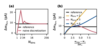
Figure 1: Distortion of synaptic-weight statistics by naive discretization. Dependence of the standard deviation $\Delta w_{N_{\text{bins}}}$ of naively discretized synaptic weights (for excitatory connections) on the number $N_{\text{bins}}$ of bins (a) and on the relative (half-)width $\left(w_{\text{max}}-\overline{w}_{\infty}\right)/\Delta w_{\text{$\infty$}}$ of the discretization interval (b). The horizontal black line marks the standard deviation $\Delta w_{\text{$\infty$}}$ of the corresponding (normal) reference weight distribution.

The optimized scheme uses the obtained knowledge of the dependence on the standard deviation to improve the discretization procedure: for each number of bins $N_{\text{bins}}$, different interval boundaries are computed such that the standard deviation is always preserved.

For $N_{\text{bins}}=2$ the optimal choice for $\left[w_{\text{min}},\,w_{\text{max}}\right]$ can be calculated analytically, yielding the interval $\left[\overline{w}_{\infty}-2\Delta w_{\text{$\infty$}},\,\overline{w}_{\infty}+2\Delta w_{\text{$\infty$}}\right]$. For any higher number of bins, not only $v_{i}$ but also $p_{i}^{*}$ in (4) depend on the interval, therefore solutions are found numerically. Here we use Brent’s method implemented in scipy.optimize.root-scalar to find the first intersection. Since the computational effort increases and yields only negligible gain for higher numbers of bins (figure 1), the optimization is only performed for $N_{\text{bins}}<2^{16}$ and for higher numbers of bins the fixed interval from (2) is used. For $N_{\text{bins}}=1$ this optimization is not possible since the standard deviation is zero by construction.

2.2 Validation procedure

2.2.1 Statistics of spiking activity

We evaluate the effects of discretized synaptic weights on network dynamics by employing the same statistical spiking-activity characteristics used in previous studies: distributions of single-neuron firing rates (FR), distributions of coefficients of variation (CV) of the interspike intervals, and distributions of short-term spike-count correlation coefficients (CC; Senk et al., 2017; Knight and Nowotny, 2018; van Albada et al., 2018; Gutzen et al., 2018; Golosio et al., 2021). The time-averaged firing rate

$$\text{FR}_{i}=\frac{N_{i}\left(T_{\text{trans}},\,T_{\text{sim}}\right)}{T_{\text{sim}}-T_{\text{trans}}}$$

of neuron $i$ is defined as the total number $N_{i}\left(T_{\text{trans}},\,T_{\text{sim}}\right)$ of spikes emitted by this particular neuron $i$ during the entire simulation, i.e., in the time interval $\left[T_{\text{trans}},\,T_{\text{sim}}\right)$, normalized by the observation duration $(T_{\text{sim}}-T_{\text{trans}})$ (Perkel et al., 1967). The interspike intervals (ISI) are the time intervals between consecutive spikes of a single neuron. From the ISI distribution, the coefficient of variation

$$\text{CV}_{i}=\frac{\sigma_{\text{ISI},i}}{\mu_{\text{ISI},i}}$$ (5)

of each neuron $i$ is computed as the ratio between the ISI standard deviation $\sigma_{\text{ISI},i}$ and its mean $\mu_{\text{ISI},i}$ (Perkel et al., 1967). The CV is a measure of the spike-train irregularity. In addition to the first-order (single-neuron) measures $\text{FR}_{i}$ and $\text{CV}_{i}$, we quantify the level of synchrony in the network on short time scales by the Pearson correlation coefficient

$$\text{CC}_{ij}=\frac{C_{ij}\left(0\right)}{\sqrt{C_{ii}\left(0\right)C_{jj}\left(0\right)}}$$ (6)

for pairs of neurons $i$ and $j$. Here,

$$C_{ij}(\tau)=\left\langle\left(x_{i}\left(t,t+\Delta\right)-\left\langle x_{i}\left(t,t+\Delta\right)\right\rangle_{t}\right)\left(x_{j}\left(t+\tau,t+\Delta+\tau\right)-\left\langle x_{j}\left(t,t+\Delta\right)\right\rangle_{t}\right)\right\rangle_{t}$$ (7)

denotes the covariance of the spike counts $x_{i/j}\left(t,\,t+\Delta\right)$ , i.e., the number of spikes in a time interval $[t,\,t+\Delta),$ for a time lag $\tau$ (Perkel et al., 1967). The bin size $\Delta$ for the covariance calculation matches the refractory period of the neurons in the model networks ($2\,\mathrm{ms}$). FR, CV and CC are calculated using the Python package NetworkUnit (Gutzen et al., 2018) which relies on the package Elephant (Denker et al., 2018).

2.2.2 Comparison of distributions

FR and CV are calculated for all neurons in each neuronal population, and the CC for all pairs of $200$ distinct neurons in each population. The model validation is based on the distributions of FR, CV and CC, respectively, obtained from these ensembles. The distributions are depicted as histograms with bin sizes $2\cdot\left(\text{IQR }/n^{1/3}\right)$ that are determined using the Freedman-Diaconis rule (Freedman and Diaconis, 1981) based on the inter-quartile range IQR and the sample size $n$. For the histograms depicted in figures 2, 3, 4, and 6, the bin size is calculated for the data obtained from the respective reference networks with continuous weight distribution, and then used for all shown distributions for one population. In figure 7, the histogram bin size is obtained from either the longest simulation ($60\,\mathrm{min}$; a–c), or from the last simulation interval ($30\text{\textendash}40\,\mathrm{min}$; d–f). While visual inspection of the histograms yields a qualitative assessment of the similarity of two distributions $p\left(x\right)$ and $q\left(x\right)$, the Kolmogorov-Smirnov (KS) score

$$D_{\text{KS}}=\sup\left|P(x)-Q(x)\right|$$ (8)

provides a quantitative evaluation. The KS score is the maximum vertical distance between the cumulative distribution functions $P(x)=\int^{x}p\left(y\right)\text{\,d}y$ and $Q(x)=\int^{x}q\left(y\right)\,\text{d}y$ (Gutzen et al., 2018) and thereby is sensitive to differences in both the shapes and the positions of the distributions.

The comparison of the distributions of FR, CV and CC for a network with continuous weights with those of a network with discretized weights eliminates other sources of variability by using the same instantiation of the random network model. The two networks not only have the same initial conditions, external inputs, connections between identical pairs of neurons, and spike-transmission delays: one by one the weights in the discretized network are the discrete counterparts of the weights in the continuous network (section 2.1).

2.3 Description of network models

The present study uses the model of the cortical microcircuit proposed by Potjans and Diesmann (2014), which mimics the local circuit below $1\,\mathrm{mm^{2}}$ of cortical surface, as a reference. Tables 1–4 provide a formal description according to Nordlie et al. (2009). The PD model organizes the neurons into eight recurrently connected populations; an excitatory (E) and an inhibitory (I) one in each of four cortical layers: L2/3E, L2/3I, L4E, L4I, L5E, L5I, L6E, and L6I. The identical current-based leaky integrate-and-fire dynamics with exponentially decaying postsynaptic currents describes the neurons of all populations. Connection probabilities $C_{YX}$ for connections from population $X$ to population $Y$ are derived from anatomical and electrophysiological measurements. The weights for the recurrent synapses are drawn from three different normal distributions ($N_{\text{distr}}=3$): mean and standard deviation are $\left(\overline{w}_{\infty},\,\Delta w_{\text{$\infty$}}\right)=\left(87.8,\,8.8\right)\,\mathrm{pA}$ for excitatory and $\left(\overline{w}_{\infty},\,\Delta w_{\text{$\infty$}}\right)=\left(-351.2,\,35.1\right)\,\mathrm{pA}$ for inhibitory connections. The weights from L4E to L2/3E form an exception as the values are doubled: $\left(\overline{w}_{\infty},\,\Delta w_{\text{$\infty$}}\right)=\left(175.6,\,17.6\right)\,\mathrm{pA}$. To account for Dale’s principle (Strata and Harvey, 1999), negative (positive) sampled weights of connections that are supposed to be excitatory (inhibitory) are set to zero. The resulting distributions are therefore slightly distorted (for the weight distributions used in this study, this distortion is negligible). Transmission delays are also drawn from normal distributions with different parameters for excitatory and inhibitory connections, respectively. Each neuron receives external input with the statistics of Poisson point process and a constant weight of $87.8\,\mathrm{pA}$. The simulations are performed with a simulation time step of $0.1\,\mathrm{ms}$ and have a duration $T_{\text{sim}}$ of $15$ biological minutes with exceptions in section 3.5. For all simulations, the first second $T_{\text{trans}}=1\,\mathrm{s}$ is discarded from the analysis. The actual observation time is therefore $T_{\text{sim}}-T_{\text{trans}}$. For easier readability all times given in this manuscript always refer to the simulation duration $T_{\text{sim}}$. The initial membrane potentials of all neurons are randomly drawn from a population-specific normal distribution to reduce startup transients.

In the original implementation of the model, the total number of synapses between two populations $S_{YX}$ is derived from an estimate of the total number of synapses in the volume and exactly $S_{YX}$ synapses are established. Section 3.3 uses this fixed total number connectivity. The fixed in-degree network models in sections 3.1 and 3.2 determine the in-degrees $K_{YX}$ by dividing the total number of synapses by the number of neurons in the target population and rounding up to the next larger integer, see (10). The rounding ensures that at least one synapse remains for a non-zero connection probability. Table 3 summarizes the resulting values of $S_{YX}$ and $K_{YX}$.

Model summary
Structure	Multi-layer excitatory-inhibitory (E-I) network
Populations	$8$ cortical in $4$ layers (L2/3, L4, L5, L6)
Connectivity	Random, independent, population-specific; fixed in-degree models and fixed total number models
Neuron model	Leaky integrate-and-fire (LIF)
Synapse model	Exponentially shaped postsynaptic currents with normally distributed static weights
Input	Independent fixed-rate Poisson spike trains to all neurons (population-specific in-degree)
Measurements	Spikes

Table 1: Description of the network model following the guidelines of Nordlie et al. (2009).

Connectivity
• Connection probabilities $C_{YX}$ from population $X$ to population $Y$ with $\{X,Y\}\in\left\{\text{L2/3,\,L4,\,L5,\,L6}\right\}\times\left\{\text{E,I}\right\}$. Values are given in Potjans and Diesmann (2014, table 5). • Self-connections (autapses) are prohibited; multiple connections between neurons (multapses) are allowed.
Fixed total number models	Total number of synapses (Potjans and Diesmann, 2014, eq. 1): $$S_{YX}=\frac{\log(1-C_{YX})}{\log((N_{Y}N_{X}-1)/(N_{Y}N_{X}))}$$ (9) In- and out-degrees are binomially distributed.
Fixed in-degree models	In-degree: $$K_{YX}=\left\lceil\frac{S_{YX}}{N_{Y}}\right\rceil$$ (10)

Neuron and synapse model
Neuron	Leaky integrate-and-fire neuron (LIF) • Dynamics of membrane potential $V_{i}\left(t\right)$ for neuron $i$: – Spike emission at times $t_{s}^{i}$ with $V_{i}\left(t_{s}^{i}\right)\geq V_{\theta}$ – Subthreshold dynamics with $\tau_{\text{m}}=R_{\text{m}}C_{\text{m}}$: $$\tau_{\text{m}}\dot{V}_{i}=-V_{i}+R_{\text{m}}I_{i}\left(t\right)\quad\text{if}\quad\forall s:\,t\notin\left(t_{s}^{i},\,t_{s}^{i}+\tau_{\text{ref}}\right]$$ (11) – Reset $+$ refractoriness: $V_{i}\left(t\right)=V_{\text{reset}}\quad\text{if}\quad\forall s:\,t\in\left(t_{s}^{i},\,t_{s}^{i}+\tau_{\text{ref}}\right]$ • Exact integration with temporal resolution $h$ (Rotter and Diesmann, 1999)
Postsynaptic currents	• Instantaneous onset, exponentially decaying postsynaptic currents • Input current of neuron $i$ from presynaptic neuron $j$: $$I_{i}\left(t\right)=\sum_{j}J_{ij}\sum_{s}\text{e}^{-\left(t-t_{s}^{j}-d_{ij}\right)/\tau_{\text{s}}}\Theta\left(t-t_{s}^{j}-d_{ij}\right)$$ (12)
Synaptic weights (reference distribution)	• Normally distributed (clipped to preserve sign): $$w_{ij}\sim\mathcal{N}\left\{\overline{w}_{\infty,YX},\,\Delta w_{\infty,YX}^{2}\right\},\,\,\,\overline{w}_{\infty,YX}=g_{YX}\cdot\overline{w}_{\infty}$$ (13)
Spike transmission delays	• Normally distributed (left-clipped at $h$): $$d_{ij}\sim\mathcal{N}\left\{\overline{d}_{X},\,\Delta d_{X}^{2}\right\}$$ (14)
Initial membrane potentials	• Normally distributed: $$V_{ij}\sim\mathcal{N}\left\{\overline{V}_{0,X},\,\Delta V_{0,X}^{2}\right\}$$ (15)

Table 2: Description of the network model (continuation of table 1).

Neuron and network parameters
Populations and external in-degree
Symbol		Value								Description
$X$		L2/3E	L2/3I	L4E	L4I	L5E	L5I	L6E	L6I	Population name
$N_{X}$		$20,683$	$5,834$	$21,915$	$5,479$	$4,850$	$1,065$	$14,395$	$2,948$	Size
$K_{X,\text{ext}}$		$1,600$	$1,500$	$2,100$	$1,900$	$2,000$	$1,900$	$2,900$	$2,100$	External in-degree
In-degrees in fixed in-degree models
$K_{YX}$		from $X$
		L2/3E	L2/3I	L4E	L4I	L5E	L5I	L6E	L6I
	L2/3E	2,200	1,080	980	468	160	0	110	0
	L2/3I	2,991	861	704	290	381	0	61	0
	L4E	160	35	1,118	795	33	1	668	0
to $Y$	L4I	1,481	17	1,814	954	17	0	1,609	0
	L5E	2,189	375	1,136	32	421	497	297	0
	L5I	1,166	160	571	13	301	405	125	0
	L6E	326	39	468	92	286	22	582	753
	L6I	767	6	75	3	137	9	980	460
Total number of synapses in fixed total number models
$S_{YX}$		from $X$
		L2/3E	L2/3I	L4E	L4I	L5E	L5I	L6E	L6I
	L2/3E	45,499,804	22,323,576	20,253,647	9,670,918	3,293,577	0	2,271,403	0
	L2/3I	17,443,694	5,018,762	4,105,338	1,690,073	2,221,212	0	353,460	0
	L4E	3,503,669	756,561	24,482,849	17,413,575	714,524	7,002	14,624,431	0
to $Y$	L4I	8,114,253	92,831	9,933,537	5,223,271	87,836	0	8,810,905	0
	L5E	10,613,575	1,817,058	5,507,804	151,900	2,040,738	2,407,889	1,438,969	0
	L5I	1,241,436	169,424	607,666	12,851	319,601	430,443	132,414	0
	L6E	4,681,225	556,108	6,727,569	1,320,233	4,112,224	305,028	837,2649	10,827,677
	L6I	2,260,836	17,207	220,032	8,078	401,637	25,217	2,888,426	1,354,319

Connection parameters and external input
Symbol	Value	Description
$\overline{w}_{\infty}$	$87.81\,\mathrm{pA}$	Reference synaptic strength. All synapse weights are measured in units of $\overline{w}_{\infty}$.
$g_{YX}$		Relative synaptic strengths:
	$1$	$X\in\left\{\text{\text{L2/3E,\,L4E,\,L5E,\,L6E}}\right\}$
	$-4$	$X\in\{\text{L2/3I,\,L4I,\,L5I,\,L6I}\}$, except for:
	$2$	$\left(X,Y\right)=\left(\text{L4E,\,L2/3E}\right)$
$\Delta w_{\infty,YX}$	$0.1\cdot g_{YX}\cdot\overline{w}_{\infty}$	Standard deviation of weight distribution
$\overline{d}_{\text{E}}$	$1.5\,\mathrm{ms}$	Mean excitatory delay
$\overline{d}_{\text{$I$}}$	$0.75\,\mathrm{ms}$	Mean inhibitory delay
$\Delta d_{X}$	$0.5\cdot\overline{d}_{X}$	Standard deviation of delay distribution
$\nu_{\text{ext}}$	$8\,\mathrm{s^{-1}}$	Rate of external input with Poisson interspike interval statistics
LIF neuron model
Symbol	Value	Description
$C_{\text{m}}$	$250\,\mathrm{pF}$	Membrane capacitance
$\tau_{\text{m}}$	$10\,\mathrm{ms}$	Membrane time constant
$E_{\text{L}}$	$-65\,\mathrm{mV}$	Resistive leak reversal potential
$V_{\theta}$	$-50\,\mathrm{mV}$	Spike detection threshold
$V_{\text{reset}}$	$-65\,\mathrm{mV}$	Spike reset potential
$\tau_{\text{ref}}$	$2\,\mathrm{ms}$	Absolute refractory period after spikes
$\tau_{\text{s}}$	$0.5\,\mathrm{ms}$	Postsynaptic current time constant

Table 3: Neuron, network, and simulation parameters.

Neuron and network parameters (cont.)
Initial membrane potentials
Symbol		Value								Description
$X$		L2/3E	L2/3I	L4E	L4I	L5E	L5I	L6E	L6I	Population name
$\overline{V}_{0,X}$		$-68.28$	$-63.16$	$-63.33$	$-63.45$	$-63.11$	$-61.66$	$-66.72$	$-61.43$	Mean in mV
$\Delta V_{0,X}$		$5.36$	$4.57$	$4.74$	$4.94$	$4.94$	$4.55$	$5.46$	$4.48$	Standard deviation in mV

Simulation parameters
Symbol	Value	Description
$T_{\text{sim}}$	$15\,\mathrm{min}$	Simulation duration
$h$	$0.1\,\mathrm{ms}$	Temporal resolution
$T_{\text{trans}}$	$1\,\mathrm{s}$	Startup transient

Table 4: Neuron, network, and simulation parameters (continuation of table 3).

2.4 Software environment and simulation architecture

The simulations in this study are performed on the JURECA supercomputer at the Jülich Research Centre, Germany. JURECA consists of 1872 compute nodes, each with two Intel Xeon E5-2680 v3 Haswell CPUs running at 2.5 GHz. The processors have 12 cores and support 2 hardware threads per core. Each compute node has at least 128$\>\mathrm{GB}$ of memory available. The compute nodes are connected via Mellanox EDR InfiniBand.

All neural network simulations in this study are performed using the NEST simulation software (Gewaltig and Diesmann, 2007). NEST uses double precision floating point numbers for the network parameters and the calculations. The simulation kernel is written in C++ but the simulations are defined via the Python interface PyNEST (Eppler et al., 2009). The simulations of the cortical microcircuit are performed with NEST compiled from the master branch (commit 8adec3c, https://github.com/nest/nest-simulator). The compilations are performed with the GNU Compiler Collection (GCC). ParaStationMPI library is used for MPI support. Each simulation runs on a single compute node with 1 MPI process and 24 OpenMP threads.

All analyses are carried out with Python 3.6.8 and the following packages: NumPy (version 1.15.2), SciPy (version 1.2.1), Matplotlib (version 3.0.3), Elephant (version 0.5.0, https://python-elephant.org), and NetworkUnit (version 0.1.0, https://github.com/INM-6/NetworkUnit).

The source code to reproduce all figures of this manuscript is publicly available at https://doi.org/10.5281/zenodo.4696168.

3 Results

In this study, the evaluation of the role of the synaptic weight resolution is based on the model of a local cortical microcircuit derived by Potjans and Diesmann (2014). The model comprises four cortical layers (L2/3, L4, L5, and L6), each containing an excitatory (E) and an inhibitory (I) neuron population. An $8\times 8$ matrix of cell-type and layer specific connection probabilities provides the basis of the connectivity between neurons (table 5 in Potjans and Diesmann, 2014). Based on this matrix, the present manuscript considers two different probabilistic algorithms to determine which individual neurons in any pair of populations are being connected. First, section 3.1 uses a fixed in-degree rule which requires for each neuron of a target population the same number of incoming connections from a source population. Second, in section 3.3 the total number of synapses between two populations is calculated and synapses are established successively until this number is reached. We refer to this latter procedure, which was also employed in the original implementation by Potjans and Diesmann (2014), as the fixed total number rule. In both algorithms, synapses are drawn randomly; the exact connectivity realization is hence dependent on the specific sequence of random numbers required for the sampling process, i.e., the choice and the seed of the employed pseudo-random number generators.

In the PD model, a spike of a presynaptic neuron elicits, after a transmission delay, a jump in the synaptic currents of its postsynaptic targets which decays exponentially with time. In the original implementation, the synaptic weights, the amplitudes of these jumps, are drawn from normal distributions when connections are established, and they remain constant for the course of the following state-propagation phase. All excitatory weights are sampled from a normal distribution with the same (positive) mean and the same standard deviation, except for connections from L4E to L2/3E where the mean and standard deviation are doubled. All inhibitory weights are sampled with a different (negative) mean and a different standard deviation.

This study compares the activity statistics obtained from simulations of a reference model with continuous weight distributions with those where the synaptic weights are drawn from the same continuous distributions and subsequently discretized. We refer to an “$N_{\text{bins}}$ discretization” as the case where the sampled weights are replaced by a finite set of $N_{\text{bins}}\in\mathcal{\mathbb{N}}^{+}$ discrete values for each of the three weight distributions. As validation measures, we use the time-averaged single-neuron firing rates (FR), the coefficients of variation (CV) of the interspike intervals as a spike-train irregularity measure, and the short-term spike-train correlation coefficients (CC) as a synchrony measure. We quantify the discretization error, i.e., the deviation between the discretized and the reference model, by the Kolmogorov-Smirnov (KS) score $D_{\text{KS}}$ computed from the empirical distributions of these statistical measures across neurons. To evaluate the significance of the discretization error, we recognize that the model is defined in a probabilistic manner: valid predictions of this model are those features that are exhibited by the ensemble of model realizations. Features that are specific to a single realization are meaningless. Therefore, deviations between realizations of a discretized and the reference model are significant only if they exceed those between different realizations of the reference model. In other words, if the observed KS score between the discretized and the reference model falls into the distribution of KS scores obtained from an ensemble of pairs of reference realizations, the weight discretization does not lead to significant errors with respect to the considered validation measure.

3.1 Naive discretization distorts statistics of spiking activity

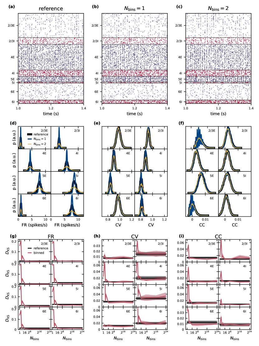
Figure 2: Effect of naive weight discretization on the spike-train statistics in networks with fixed in-degrees. Caption continued on next page.

(a)–(c): Spiking activity (dots mark time and sender of each spike) of $5\%$ of all excitatory (blue) and inhibitory (red) neurons of the eight neuronal populations (vertically arranged) of the PD model with fixed in-degrees. Spike times from simulations of the reference network (a) and of networks with naively discretized $1$-bin (b) and $2$-bin weights (c). (d)–(f): Population-specific distributions of single-neuron firing rates FR (d), coefficients of variation CV of the interspike intervals (e), and spike-train correlation coefficients CC (f) from simulations of the reference network (black), as well as networks with $1$-bin (blue) and $2$-bin weights (yellow). (g)–(i): Mean (solid curves) and standard deviation (shaded areas) of the Kolmogorov-Smirnov scores $D_{\text{KS}}$ obtained from distributions in panels (d)–(f) across five different network realizations. Red: Comparison of simulation results with discretized ($N_{\text{bins}}=1,\ldots,2^{24}$ ) and reference weights (with identical random-number generator seed). Black: Comparison of different random realizations of the reference network.

The connectivity of the PD model exhibits different sources of heterogeneity: connections between pairs of neurons result from a random process and distributions govern the creation of their weights and delays. A number of previous studies have shown how such heterogeneities influence neuronal network dynamics (Tsodyks et al., 1993; Golomb and Rinzel, 1993; van Vreeswijk and Sompolinsky, 1998; Neltner et al., 2000; Denker et al., 2004; Roxin et al., 2011; Roxin, 2011; Pfeil et al., 2016). In particular, distributed in-degrees, as implemented with the fixed total number rule in the original version of the model by Potjans and Diesmann (2014), can obscure effects of altered weight distributions which are the primary subject of this study. To isolate the role of the weight distribution, we therefore start by investigating a fixed in-degree version of the PD model. To assess how a discretization of the weights affects the spiking activity in the network, we begin with a simple “naive” discretization scheme: an arbitrary interval is defined around the mean value of the underlying normal distribution (here: $\pm 5$ standard deviations) and discretized into a desired number of bins. Each weight sampled from the continuous distribution is replaced by the nearest bin value, respectively (for details, see section 2.1).

We use similar measures and procedures as previous studies (e.g., van Albada et al., 2018; Knight and Nowotny, 2018) to compare the activity on a statistical level, but with the major difference that here the network is simulated longer, in fact $15$ minutes of biological time (see section 3.5). The raster plots in figure 2(a–c) show qualitatively similar asynchronous irregular spiking activity in all neuronal populations. The individual spike times, however, are different in the networks with synaptic weights using the reference implementation with double precision in panel (a) and in the networks with $1$- and $2$-bin weights in panels (b) and (c), respectively. The dynamics of recurrent neuronal networks similar to the PD model is often chaotic (Sompolinsky et al., 1988; van Vreeswijk and Sompolinsky, 1998; Monteforte and Wolf, 2010). Even tiny perturbations (such as modifications in synaptic weights) can therefore cause large deviations in the microscopic dynamics. Macroscopic characteristics such as distributions of firing rates, spike-train regularity and synchrony measures, however, should not be affected. Preserving the spiking statistics upon weight discretization is therefore an aim of this study.

The distributions of time-averaged firing rates obtained with $1$-bin weights have a similar mean as the reference distribution, but are more narrow in all populations (figure 2d). In homogeneous networks with non-distributed $1$-bin weights, analytical studies predict that all neurons inside one population have the same firing rate (Brunel, 2000; Helias et al., 2014), in contrast to the reference network with distributed weights and an expected rate distribution of finite width. The remaining finite width of the rate distribution obtained from network simulations with $1$-bin weights is a finite-size effect and decreases further for larger networks and longer simulation times. For $2$-bin weights generated by this naive discretization scheme, the rate distributions are broader than in the reference network (figure 2d). For several neuronal populations, such as L2/3E or L2/3I, the distributions of the coefficients of variation of the interspike intervals obtained from networks with discrete weights are similar to those of the reference network (figure 2e). In other populations, such as L6I, the CV distributions are narrower for $1$-bin weights and broader for $2$-bin weights, while the mean is preserved. The distributions of correlation coefficients in the discretized implementations are similar to the reference version for most populations (figure 2f). Only in L2/3E and L6E we see an oscillatory pattern for one bin in the region of small correlations. The same oscillatory pattern is also present in the CC distribution of the reference network but less pronounced (not visible here).

To quantify the differences in the resulting distributions we use the Kolmogorov-Smirnov (KS) score. In each case we compare the distributions of FR, CV and CC obtained from simulations of networks with binned weights to the reference distributions. To assess the significance of non-zero KS scores, we repeat the comparison analysis for pairs of (random) realizations of the reference network (i.e., different realizations of the connectivity, spike-transmission delays, external inputs, and initial conditions). As simulation results should not qualitatively depend on the specific realization of the probabilistically defined model, all deviations (KS scores) which are of the same size as or smaller than this baseline are insignificant. For all three activity statistics (FR, CV, CC) the deviations are largest for one and two bins (figure 2g–i). For around $16$ bins the deviations in all three activity statistics converge towards a non-zero KS score, and do not decrease further with any higher number of bins. This residual deviation is the minimal possible deviation for this simulation time. In the fixed in-degree network using the naive discretization scheme, these deviations are smaller than the baseline obtained using different network realizations from $16$ bins onward. For the kind of network simulation studied here and the specific choice of the binning, $16$ bins are therefore sufficient to achieve activity statistics with a satisfactory precision. For lower numbers of bins, a pattern appears in all populations and for all three statistical measures: the deviations from the reference network do not decrease monotonously with increasing number of bins, but increase from one to two bins, decrease from two to three, and increase again from three to four bins (figure 2g–i). These differences are highly significant as in several neuronal populations three bins achieve a score value better than the reference obtained using different seeds while four bins do not. The weight discretization procedure (section 2.1) reveals a hint on the origin of this behavior. The naive discretization scheme changes the standard deviation of the weight distributions depending on the number of bins. Three bins achieve a good result by a mere coincidence, because due to the choice of the binning interval, the standard deviation of the discrete weights is close to the standard deviation of the reference distributions (see figure 1). Comparing the KS scores in figure 2(g) with the discrepancies between the standard deviations in figure 1(a) exhibits the same pattern in both measures.

3.2 Optimized discretization preserves statistics of spiking activity

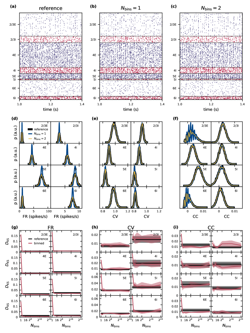
Figure 3: Effect of optimized weight discretization on the spike-train statistics in networks with fixed in-degrees. Same display as in figure 2.

Suspecting that a discrepancy between the standard deviations of the weight distributions in the reference and the binned network results in deviant activity statistics, we derive a discretization method that preserves the standard deviation of the reference weights for any number of bins. This method adapts the width of the interval in which the discrete bins are evenly placed, depending on the number of bins and the reference weight distribution (section 2.1). If the discrepancy in the standard deviations of the weight distributions is indeed the major cause of the errors observed in the activity statistics, the optimized discretization method should substantially reduce these errors. In the $1$-bin case the standard deviation is per definition zero and the optimization procedure cannot be applied. Similarly the optimization procedure is not applied in the cases with $2^{16}$and $2^{24}$ bins. Therefore, the shown data for $1,\,2^{16},\text{ and }2^{24}$ bins are the same in figures 2 and 3. Already for two bins, the FR, CV and CC distributions resulting from the optimized discretization visually match the distributions from the reference network in all neuronal populations in figure 3(d–f) in contrast to figure 2(d–f). The KS score confirms that the optimized discretization improves the accuracy of simulation with low numbers of bins (figure 3g–i). A discretization using two bins is sufficient to yield scores of the same order as or even smaller than the baseline resulting from the comparison of different realizations of the reference network. Increasing the number of bins beyond two does not lead to any further improvements for CV and CC. The KS score for the FR decreases slightly (not visible here) up to around $16$ bins, from where it remains stationary for all higher number of bins. For the fixed in-degree version of the PD model, the accuracy of the simulation is therefore preserved with a $2$-bin weight discretization.

3.3 Minimal weight resolution depends on in-degree heterogeneity

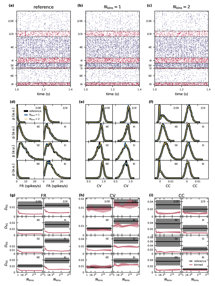
Figure 4: Effect of optimized weight discretization on the spike-train statistics in networks with fixed total numbers of connections. Same display as in figure 2.

So far we studied the PD model with fixed in-degrees. In this section we move on to a model version in which the neuronal populations are connected with the fixed total number rule (as originally used by Potjans and Diesmann, 2014), leading to binomial distributions of the numbers of incoming connections per neuron in each population. In comparison to the networks used in sections 3.1 and 3.2, this distribution of in-degrees leads to a heterogeneity across neurons inside one population independent of the weight distributions. We use the optimized discretization scheme and employ the same statistical analysis as in the previous section, to determine how this additional network heterogeneity influences the accuracy of network simulations subject to weight discretization.

In figure 4(d–f), the distributions of firing rates, coefficients of variation of the interspike intervals and correlation coefficients using reference weights have different shapes and in most populations increased widths compared to the distributions in the previous fixed in-degree network in figure 3(d–f). For all three statistics (FR, CV, CC) the distributions of the binned network match those of the reference network closely for one and two bins (figure 4d–f). As before, we quantify the deviations of the simulations with the binned weights from the reference using the KS score (figure 4g–i). For CV and CC, the score shows no systematic trend with varying number of bins. For the FR, there is a small descend from one to around $16$ bins and a stationary score for all higher numbers of bins. Nevertheless for all three statistical measures the score values are always smaller or of similar order as the disparity between different realizations of the reference network. We conclude that already just one bin successfully preserves the activity statistics in the PD model with distributed in-degrees and using the optimized discretization method this remains true also for higher numbers of bins.

3.4 Mean-field theory relates variability of weights, in-degrees and firing rates to minimal weight resolution

Two weight bins preserve the activity statistics of the PD model in the fixed in-degree network (section 3.2) and one weight bin is sufficient for the network with heterogeneous in-degrees (section 3.3). This observation calls for a deeper look at the influence of weight and in-degree heterogeneity on the firing statistics. In mean-field approximation (Fourcaud and Brunel, 2002; Schuecker et al., 2015), the stationary firing response of a neuron $i$ with exponential postsynaptic currents is fully determined by the first two cumulants

$$\mu_{i} = \tau_{\text{s}}\sum_{j\in X_{i}}w_{ij}\nu_{j},$$ (16)

$$\sigma_{i}^{2} = \tau_{\text{s}}\sum_{j\in X_{i}}w_{ij}^{2}\nu_{j},$$ (17)

of its total synaptic input current. Here, $X_{i}$ denotes the population of neurons presynaptic to $i$, $\nu_{j}$ the stationary firing rate of presynaptic neuron $j$, $w_{ij}$ the synaptic weight, and $\tau_{\text{s}}$ the synaptic time constant. The size of the presynaptic population $X_{i}$ defines the in-degree $K_{i}=|X_{i}|$ of neuron $i$. Any heterogeneity in $w_{ij}$ and $K_{i}$ (and $\nu_{j})$ leads to a heterogeneous synaptic input statistics $\mu_{i}$ and $\sigma_{i}^{2}$, and, in turn, to a heterogeneous firing statistics. Here, we therefore argue that weight discretization preserves the firing statistics across the population as long as it preserves the synaptic-input statistics across the population. Rather than developing a full self-consistent mathematical description of this statistics (Roxin et al., 2011; van Vreeswijk and Sompolinsky, 1998; Renart et al., 2010; Helias et al., 2014), we restrict ourselves to studying the effect of weight discretization on the ensemble statistics of the synaptic-input mean $\mu_{i}$ and variance $\sigma_{i}^{2}$, under the assumption that the distributions of $w_{ij}$, $K_{i}$ and $\nu_{j}$ are known. For simplicity, we limit this discussion to the first two cumulants of the ensemble distributions, the ensemble mean $\left\langle x\right\rangle$ and variance $\left\langle\delta x^{2}\right\rangle$ of $\mu_{i}$ and $\sigma_{i}^{2}$ ($x\in\left\{\mu_{i},\sigma_{i}^{2}\right\}$):

$$\left\langle\mu\right\rangle = \tau_{\text{s}}\left\langle K\right\rangle\left\langle w\right\rangle\left\langle\nu\right\rangle,$$ (18)

$$\left\langle\sigma^{2}\right\rangle = \tau_{\text{s}}\left\langle K\right\rangle\left(\left\langle w\right\rangle^{2}+\left\langle\delta w^{2}\right\rangle\right)\left\langle\nu\right\rangle,$$ (19)

$$\left\langle\delta\mu^{2}\right\rangle = \tau_{\text{s}}^{2}\left[\left\langle\delta K^{2}\right\rangle\left\langle w\right\rangle^{2}\left\langle\nu\right\rangle^{2}+\left\langle K\right\rangle\left\langle w\right\rangle^{2}\left\langle\delta\nu^{2}\right\rangle+\left\langle K\right\rangle\left\langle\delta w^{2}\right\rangle\left(\left\langle\nu\right\rangle^{2}+\left\langle\delta\nu^{2}\right\rangle\right)\right],$$ (20)

$$\left\langle\delta\left(\sigma^{2}\right)^{2}\right\rangle = \tau_{\text{s}}^{2}\left[\left(\left\langle\delta K^{2}\right\rangle-\left\langle K\right\rangle\right)\left(\left\langle w\right\rangle^{2}+\left\langle\delta w^{2}\right\rangle\right)^{2}\left\langle\nu\right\rangle^{2}+\left\langle K\right\rangle\left\langle w^{4}\right\rangle\left(\left\langle\nu\right\rangle^{2}+\left\langle\delta\nu^{2}\right\rangle\right)\right].$$ (21)

The above expressions rely on Wald’s equation (Wald, 1944), the Blackwell-Girshick equation (Blackwell and Girshick, 1946), and general variance properties. Note that in previous works on heterogeneous networks, the population variance $\left\langle\delta\left(\sigma^{2}\right)^{2}\right\rangle$ of the input variance is often neglected (Roxin et al., 2011; Helias et al., 2014; Renart et al., 2010). Roxin et al. (2011) moreover neglect the dependence of $\left\langle\sigma^{2}\right\rangle$ on the weight variance $\left\langle\delta w^{2}\right\rangle$. While the ensemble measures in (18)–(21) can be computed for the whole neuronal network, it is more conclusive to use population-specific ensemble measures computed individually for each pair of source $X$ and target population $Y$. With this approach, $\left\langle K\right\rangle$ and $\left\langle\delta K^{2}\right\rangle$ refer to the mean and the variance of the number of inputs from population $X$ across all neurons in the target population $Y$, $\left\langle w\right\rangle$ and $\left\langle\delta w^{2}\right\rangle$ to the mean and the variance of the weights of all connections from $X$ to $Y$, and $\left\langle\nu\right\rangle$ and $\left\langle\delta\nu^{2}\right\rangle$ to the mean and the variance of the firing rate across neurons in the source population $X$. Deriving these population-specific measures is possible because $\mu$ and $\sigma^{2}$ given in (16) and (17), respectively, decompose into the contributions of the different source populations. Besides, we assume that $K_{i}$ and $w_{ij}$ are drawn independently from their respective distributions and the rates $\nu_{j}$ are also assumed to be independent.

For each of the ensemble measures (18)–(21), we define a discretization error

$$\varepsilon_{N_{\text{bins}}}\left(x\right)=\frac{\left|x_{\infty}-x_{N_{\text{bins}}}\right|}{\left|x_{N_{\text{bins}}}\right|}$$ (22)

as the normalized deviation of the measure $x_{N_{\text{bins}}}$ in a network with $N_{\text{bins}}$ weight bins from its counterpart $x_{\infty}$ in the network with the reference weight distribution. In table 5, we summarize $\varepsilon_{N_{\text{bins}}}$ for all four ensemble measures to assess deviations introduced by weight discretization to one and two bins according to the optimized scheme. In the $2$-bin case, $\left\langle w\right\rangle$ and $\left\langle\delta w^{2}\right\rangle$ are the same for the reference and binned networks; in the $1$-bin case, however, only $\left\langle w\right\rangle$ is preserved while $\left\langle\delta w^{2}\right\rangle$ vanishes by definition. The term $\left\langle w^{4}\right\rangle$ in (21) evaluates for the normal reference weight distribution to $\left\langle w\right\rangle^{4}+6\left\langle w\right\rangle^{2}\left\langle\delta w^{2}\right\rangle+3\left\langle\delta w^{2}\right\rangle^{2}$, for one bin to $\left\langle w\right\rangle^{4}$, and for two bins to $\left\langle w\right\rangle^{4}+6\left\langle w\right\rangle^{2}\left\langle\delta w^{2}\right\rangle+\left\langle\delta w^{2}\right\rangle^{2}$. Therefore, the results in the fourth column of table 5 are only valid for a normal reference weight distribution, while the first three columns are valid independent of the shape of the weight, in-degree, or firing rate distribution. For simplicity, the rate distributions are here assumed to be similar in the reference and the binned networks. The mean-field theory in general relates the fluctuating synaptic input to the distribution of output spike rates by a self-consistency equation such that any change of parameters changes both. Here we go with the assumption of similarity as we are interested in finding binned networks yielding similar spiking statistics as the reference. Consequently, $\varepsilon_{1}\left(\left\langle\mu\right\rangle\right)=\varepsilon_{2}\left(\left\langle\mu\right\rangle\right)=\varepsilon_{2}\left(\left\langle\sigma^{2}\right\rangle\right)=\varepsilon_{2}\left(\left\langle\delta\mu^{2}\right\rangle\right)=0$, since all these measures only depend on quantities which are the same in networks with the reference weight distribution and their binned counterparts. Non-zero table entries result from cases where the respective quantities do not cancel.

$x$	$\left\langle\mu\right\rangle$	$\left\langle\sigma^{2}\right\rangle$	$\left\langle\delta\mu^{2}\right\rangle$	$\left\langle\delta\left(\sigma^{2}\right)^{2}\right\rangle$
$\varepsilon_{1}\left(x\right)$	$0$	$j$	$j\cdot\frac{1+f}{k+f}$	$j\cdot\left(2+j\right)\cdot\left(1+2\frac{1+f}{k+f}\right)$
$\varepsilon_{2}\left(x\right)$	$0$	$0$	$0$	$\frac{2j^{2}}{4j+\frac{k+f}{1+f}\left(1+j\right)^{2}}$

Table 5: Discretization error of the synaptic-input statistics for 1- and 2-bin discretization. Discretization error $\varepsilon_{N_{\text{bins}}}(x)$ as defined in (22) for the four ensemble measures (18)–(21) (columns), for networks with $N_{\text{bins}}=1$ and $N_{\text{bins}}=2$ weight bins (rows). The parameters $j:=\left\langle\delta w^{2}\right\rangle/\left\langle w\right\rangle^{2}$, $f:=\left\langle\delta\nu^{2}\right\rangle/\left\langle\nu\right\rangle^{2}$ and $k:=\left\langle\delta K^{2}\right\rangle/\left\langle K\right\rangle$ denote the squared variation coefficients of the synaptic weights and the firing rates, and the Fano factor of the in-degrees, respectively.

Conventional mean-field theory captures the mean and the variance of the input fluctuations to describe the dynamical state of a recurrent random spiking neuronal network. This is sufficient to predict characteristics of network dynamics like the mean spike rate, the pairwise correlation between neurons, and the power spectrum. Therefore, if the deviations in table 5 of $\mu$ and $\sigma^{2}$ are small, the activity statistics in the network are expected to be preserved. Right off the bet, the $2$-bin discretization seems more promising, because three of the four ensemble averages considered here evaluate to zero by definition. This holds true for any in-degree, weight or firing rate distribution as long as the $2$-bin discretization preserves mean and standard deviation of the weight distribution. In the $1$-bin case, the deviation of $\left\langle\sigma^{2}\right\rangle$ still depends on the spread of synaptic weights without any further additive terms or scaling. In particular, the term does not depend on whether the in-degrees are distributed or not. In networks with a large spread of synaptic weights, a $1$-bin weight discretization is therefore always insufficient. The third column of table 5 considers $\left\langle\delta\mu^{2}\right\rangle$, the variance of the means of the membrane potential across the population. Again, the deviation of this value from the reference evaluates to exactly zero for the $2$-bin case. For a single bin, however, a more complex term remains. For small or no variability in the number of incoming synapses, the deviation of $\left\langle\delta\mu^{2}\right\rangle$ in the $1$-bin case depends on the width of the weight distribution, but the more the in-degrees are distributed, the smaller this dependence becomes; for a high variability of the in-degree $k\rightarrow\infty$ with $k:=\left\langle\delta K^{2}\right\rangle/\left\langle K\right\rangle$ the deviation goes to zero even in the $1$-bin case. In that case, the variability of the mean membrane potentials caused by the distributed in-degrees is so large that the variability of the weight distribution does not matter. The deviations of $\left\langle\delta\left(\sigma^{2}\right)^{2}\right\rangle$, which quantify the variability of the magnitude of the membrane potential fluctuations across populations, are non-zero for both $1$- and $2$-bin discretization. For one bin, a high in-degree variability $k\rightarrow\infty$ leads to a residual deviation $j\cdot\left(2+j\right)$ that only depends on the relative spread $j:=\left\langle\delta w^{2}\right\rangle/\left\langle w\right\rangle^{2}$ of the reference weight distribution. For two bins, the respective deviation declines with an increasing variability of the in-degrees.

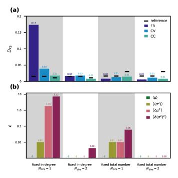
Figure 5: Statistics of spiking activity and discretization errors of the synaptic-input statistics. (a): Mean over all neuron populations of the $D_{\text{KS}}$ scores (for one fixed network realization) calculated as in figures 3 and 4 for FR (dark blue), CV (light blue), and CC (turquoise). Mean reference is shown in black. (b): Mean over all pairs of source and target populations of $\varepsilon$ values calculated as in table 5 for the averaged input mean $\left\langle\mu\right\rangle$ (green), averaged input variance $\left\langle\sigma^{2}\right\rangle$ (olive green), the population variance of the input mean $\left\langle\delta\mu^{2}\right\rangle$ (rose), and the population variance of the input variance $\left\langle\delta\left(\sigma^{2}\right)^{2}\right\rangle$ (purple). Logarithmic $y$-axis used for $\varepsilon$. First column: fixed in-degree network with $1$-bin weights. Second column: fixed in-degree network with $2$-bin weights. Third column: fixed total number network with $1$-bin weights. Fourth column: fixed total number network with $2$-bin weights. All $\varepsilon$ values vanishing by construction are marked as “$0$” without decimals, all others are rounded to two decimal places.

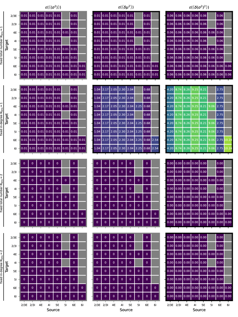
Figure 8: Discretization errors of the synaptic-input statistics in mean-field approximation. Caption continued on next page.

For a direct comparison of the theoretical approach and results obtained from analyzing simulated data, we evaluate the terms in table 5 with parameters and simulation results of our tested network models with optimized weight discretization (figures 3 and 4). The contributions of the firing rates are numerically computed based on measured firing rates from simulations with the reference weight distribution. Figure 5 is arranged such that the KS scores of the simulated spiking activity in panel (a) can be directly compared to the computed deviations in the neuron input fluctuations in panel (b) for the fixed total number and fixed in-degree networks with one and two weight bins. Both the KS scores and the $\varepsilon$ values are here averaged over populations; for completeness, figure 8 shows all $\varepsilon$ values for each pair of source and target population individually. In the PD model (Potjans and Diesmann, 2014), the standard deviations of the weights are $10\%$ of the mean values, resulting in $j=0.01$. With fixed total number connectivity (multapses allowed), the in-degrees are binomially distributed with a mean of $S_{YX}/N_{Y}$ and a variance of $S_{YX}/N_{Y}\left(1-1/N_{Y}\right)$, where $S_{YX}$ is the total number of synapses between source $X$ and target population $Y$, and $N_{Y}$ is the number of neurons in the target population (Senk et al., 2020). The Fano factor of the in-degrees is therefore $k=1-1/N_{Y}$. The fixed in-degree scenario simplifies $k=0$ as $\left\langle\delta K^{2}\right\rangle=0$.

In the fixed total number network with one weight bin, the normalized deviations of all of the considered ensemble measures are very small ($\varepsilon_{1}<0.1$). This is in line with the corresponding KS scores of the spiking activity being all below the reference. In contrast, the fixed in-degree network using one weight bin exhibits large discretization errors: values above $1$ for $\left\langle\delta\mu^{2}\right\rangle$ and even above $10$ for $\left\langle\delta\left(\sigma^{2}\right)^{2}\right\rangle$ are observed in some populations. These deviations explain the differences in spiking statistics seen in figure 5(a). Using two weight bins, all considered ensemble averages have negligible deviations corroborating the respective observations of negligible deviations in simulation activity statistics.

3.5 Observation duration determines specificity of validation measures and validation performance

3.5.1 Specificity of validation measures

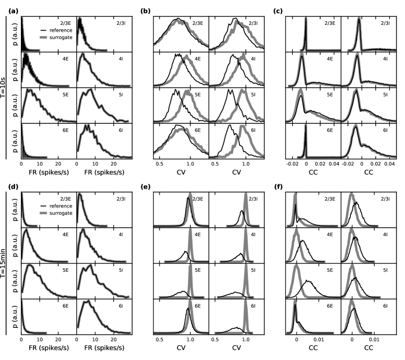
Figure 6: Role of observation duration for the specificity of validation measures. Distributions of population-specific single-neuron firing rates FR (a,d), coefficients of variation CV of the interspike intervals (b,e), and spike-train correlation coefficients CC (c,f). Black: fixed total number network model with reference weight distribution (same as in figure 4). Gray: surrogate data with randomized spike times (see text). Top: observation duration $T_{\text{sim}}=10\,\mathrm{s}.$ Bottom: $T_{\text{sim}}=15\,\mathrm{min}$.

The criteria that are naturally used to validate a particular model implementation are determined by those features the model seeks to explain. The validation metrics should therefore reflect the specifics of the model, rather than effects that arise from other aspects not directly related to the model under investigation. The example of this study, the model by Potjans and Diesmann (2014), predicts that layer and population specific patterns of firing rates, spike-train irregularities (ISI CVs) and pairwise correlations are a consequence of the cell-type specific connectivity within local cortical circuits. Distributions of these quantities therefore constitute meaningful validation metrics for this model. However, this holds only true if these distributions are obtained such that they primarily reflect the model-specific connectivity, and are not the result of some other trivial effects, for example those introduced by the measurement process. A standard approach to disentangle such effects is to compare the data generated by the model against those generated by an appropriate null hypothesis where certain model-specific features are purposefully destroyed (see Grün (2009) for a review of methods for spiking activity and their limitations).

As an example, consider the distributions of spike-train correlation coefficients. The PD model predicts that pairwise spike-train correlations are small and distributed around some population-specific non-zero mean, and that these distributions are explained by the specifics of the connectivity. Consider now the alternative hypothesis (null hypothesis) according to which the correlation distributions are fully explained by the distributions of time-averaged firing rates, and do not reflect any further characteristics of the synaptic connectivity. An instantiation of this null hypothesis is obtained by generating surrogate data from the model data, where the spike times for each neuron are uniformly randomized within the observation interval. Under this null hypothesis, the distributions of firing rates are fully preserved (figure 6a and d), but the pairwise correlations on a millisecond timescale (as well as spike-train regularities) are destroyed. For increasing observation time $T_{\text{sim}}\to\infty$, the distributions of correlation coefficients hence approach delta-distributions with zero mean. For finite sample sizes, i.e., finite observation duration $T_{\text{sim}}$, however, spurious non-zero correlations remain. The correlation distributions obtained under this null hypothesis therefore have some finite width, and may be hard to distinguish from the actual model distributions. Indeed, the distributions of spike-train correlation coefficients obtained from $T_{\text{sim}}=10\,\mathrm{s}$ simulations of the PD model cannot be distinguished from those generated by the null hypothesis introduced above (figure 6c). Only for sufficiently long observation intervals do the empirical model correlation distributions carry specific information about the network connectivity which is not already contained in the rate distributions (figure 6(f) for $T_{\text{sim}}=15\,\mathrm{min}$).

We conclude that a model validation based on spike-train correlation distributions should be interpreted with care: for short observation duration (e.g., $T_{\text{sim}}=10\,\mathrm{s}$ as used by van Albada et al., 2018, Knight and Nowotny, 2018, Rhodes et al., 2019, and Golosio et al., 2021), any model implementation that preserves the rates but destroys interactions between spike trains would not differ from the reference model with respect to the correlation distributions. Distributions of correlations obtained from short observation periods may however still be useful to rule out that some model implementation erroneously generates correlations that are significantly larger than those generated by the reference model (see, e.g., Pauli et al., 2018).

In principle, the same is true for other validation metrics, such as distributions of interspike intervals (ISI) and their coefficients of variation CVs (definitions in section 2.2.1, figure 6b and e). The surrogate data of this example may suggest all CVs to be one, but the finite sample sizes lead to distributions of finite widths and eventually even a shifted mean (as seen in the $T_{\text{sim}}=10\,\mathrm{s}$ case). In the face of finite observation times, one needs to check to what extent these metrics are informative about the specifics of the underlying model, and whether there is actually any chance that some imperfect implementation of the model can lead to deviations from the reference. The comparison with appropriate surrogate data is a straight forward and established procedure to test this. In the following subsection, we employ an alternative approach and investigate directly how the validation performance converges with the length of the observation interval.

3.5.2 Validation performance

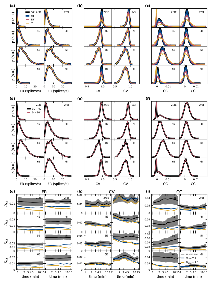
Figure 7: Dependence of validation performance on observation interval and duration. Caption continued on next page.

(a)–(f): Population specific distributions of single-neuron firing rates FR (a,d), coefficients of variation CV of the interspike intervals (b,e), and spike-train correlation coefficients CC (c,f) for different observation durations ($5$, $15$, $40$, $60\,\textmd{min}$; a-c) and different observation intervals ($[0,10]\,\textmd{min}$, $[30,40]\,\text{min}$) with identical duration (d-f). (g)–(i): Dependence of validation performance (Kolmogorov-Smirnov score $D_{\text{KS}}$ of distributions obtained from simulations with discretized and double-precision weights) for single-neuron firing rates FR (g), coefficients of variation CV of the interspike intervals (h), and spike-train correlation coefficients CC (i) on observation duration $T_{\text{sim}}$ with $1$-bin (blue) and $2^{24}$-bin weights (yellow). Black traces and gray band represent mean and standard deviation of KS scores computed with pairs of five random realizations of the reference model.

Here, we tackle the question of how long simulations need to be to yield an amount of data that is sufficient for exposing model specifics beyond effects of finite data (see also Dahmen et al. (2019) for a discussion). To investigate the convergence behavior of our validation metrics, we analyze simulated data of up to one hour of model time of the PD model (figure 7a–c). A completely converged distribution is defined as independent of time when its shape does not change any more if more data is added. Firing-rate distributions converge fast; no difference is visible if analyzing only $5\,\mathrm{min}$ of the data or the full hour. In contrast, the shape of the distributions of correlation coefficients still changes after $40\,\mathrm{min}$ for all populations and appears not to have converged for the entire data recorded. The behavior of the distributions of the coefficients of variation is population-specific: a higher on-average firing rate leads to more spike data entering the computation of the CVs which results in a faster convergence with simulated model time. The convergence of distributions from low-firing neurons in L2/3E, L2/3I and L6E, for instance, is slow.

To rule out that the underlying network dynamics change qualitatively over time, which would have been a simple explanation for changes in the distributions, we compare data from two $10\,\mathrm{min}$ intervals separated by $20\,\mathrm{min}$: the distributions match for all three metrics (figure 7d–f). Convergence of the network dynamics to a stationary state happens in fact on a much smaller time scale in the PD model network, and we avoid distortions due to startup transients by always excluding the very first $T_{\text{trans}}=1\,\mathrm{s}$ of each simulation from the data analyzed. To achieve the same interval lengths, also the first second of the $[30,40]\,\text{min}$ interval is excluded.

These findings make it apparent that only comparisons between simulations of equal model time intervals are meaningful. Choosing a sufficient length for the time intervals such that model specifics are not overshadowed by finite-data effects is a non-trivial task which depends on the network model itself but also on the statistical measures applied, as shown in figures 6 and 7. There are a couple of possible approaches for this endeavor:

1. The conceptually easiest way is to simulate for very long periods of biological times (e.g., more than one hour) until all calculated statistical distributions are converged. Because most complex neuronal network simulations require wall-clock times much longer than the model time simulated on modern HPC systems, this approach is unfeasible until accelerated hardware is available (Jordan et al., 2018).

2. Otherwise one can restrict the analysis to statistics that are less impacted by finite data biases (e.g., the time-averaged firing rate in figure 7a). The drawback of this approach is that a thorough validation relies on a number of complementary metrics as decisive model-specific differences may only become evident with some measures and not others (Senk et al., 2017).

3. One can also derive analytical relations for the convergence behavior of certain observables and fit them to a series of differently long simulations. In this way the true value of the observable can be estimated without finite data biases, as was, e.g., performed in Dahmen et al. (2019).

4. The strategy employed in this study is the following: if qualitative findings are the important parts of the study, then one can first guess a long enough simulation time and perform the study with this. Afterwards one has to confirm that the specific measurements to uphold these findings are already converged also for shorter time scales than employed in the study. Figure 7(g)–(i) shows the KS scores obtained for a network with fixed total number connections but for different simulation durations. Also for shorter simulation times than $15\,\mathrm{min}$ the score of a simulation with one bin is below the reference and therefore has acceptable accuracy, while the improvement in accuracy when going to a high number of bins is only small. The drawback of this approach is that one can only confirm in retrospective if the chosen simulation time was sufficient enough, but if one finds the opposite one would have to perform the analysis again for longer simulation times.

4 Discussion

This study contributes to the understanding of the effects of discretized synaptic weights on the dynamics of spiking neuronal networks. We found the lowest weight resolution that can maintain the original activity statistics for two derivatives of the cortical microcircuit model of Potjans and Diesmann (2014). In general, the discretization procedure must preserve the moments of the reference weight distributions. In networks where all neurons within one population receive the same number of synaptic inputs, the variability in synaptic weights constitutes the dominant source of input heterogeneity. In this case, the weight discretization has to account for both the mean and the variance of the normal reference weight distributions. In such networks, two discrete weights are sufficient for each pair of populations to preserve the population-level statistics. In networks where the neurons inside the same neuronal population receive different numbers of inputs, the variability in in-degrees may play a major role in the population-level statistics. In the PD model with binomially distributed in-degrees, the in-degree variability is dominating the weight variability such that the original weights can be replaced by their mean value without changing the population-level statistics. The study outlines a mean-field theoretical approach to relate synaptic weight and in-degree heterogeneities to the variability of the synaptic input statistics which, in turn, determines the statistics of the spiking activity. We show that this relationship qualitatively explains the effects of a reduced synaptic weight resolution observed in direct simulations. Finally the work sheds light on the convergence time of the activity statistics. For a meaningful validation, the simulated model time needs to be long enough such that the statistics are not dominated by effects of finite sample sizes and instead are sufficiently sensitive to distinguish model specifics from random outcomes.

In our approach synaptic weights are stored with the full floating point resolution the computer hardware supports and all computations are carried out using the full resolution of the floating point unit of the processor. Discretization just refers to the fact that a synaptic weight only assumes one of a small set of predefined values. Thus, for the price of an indirection, only as many bits are required per synapse as needed to uniquely identify the values in the set: one bit for two values, 2 bit for four values. In the cortical microcircuit model of Potjans and Diesmann (2014), the recurrent weights are drawn from one of three distinct distributions (section 2.3). As these weights can be replaced by the respective mean weight without affecting the activity statistics, it is sufficient to store only three distinct weight values (one for each synapse type) rather than the weights for all existing synapses. Based on the $64$-bit required for the representation of each weight of the $298,880,941$ recurrent connections in the cortical microcircuit model with fixed total number connectivity, this reduces the memory demand of the network by $2.39\,\mathrm{GB}$. This reduction scales linearly with the number of synapses, such that the memory saving potential increases for larger networks. In our reference implementation NEST this can be achieved by using three synapses models derived from the static_synapse_hom_w class. If several weights are required for each group of neurons, as is the case for fixed in-degree connectivity, there exists at present no pratical implementation in NEST or neuromorphic hardware that can fully utilize a similar memory saving potential. More research is required on suitable interfaces for the user, the domain specific language NESTML (Plotnikov et al., 2016) offers a perspective.

The synaptic weight resolution can be substantially reduced if the discretization procedure accounts for the statistics of the reference weights. Simulation architectures which allow users to adapt the synaptic weight resolution to the specific network model are therefore preferable to those where the weight representation is fixed. This seems to advocate the use of a mixed precision approach in neuromorphic hardware, in which the synaptic weights are implemented with a lower resolution while the computations are performed with higher numerical precision. An opportunity for future development is to determine which calculation precision is required. While it is possible to achieve comparable network dynamics with 32-bit fixed point arithmetic (van Albada et al., 2018), a minimum bit limit has not been identified, yet.

This study is restricted to non-plastic neuronal networks that fulfill the assumptions underlying mean-field theory as presented, e.g., in (Brunel, 2000), including heterogeneous networks as studied in (Roxin et al., 2011). In such networks, the distribution of synaptic inputs across time can be approximated by a normal distribution (diffusion approximation) such that the statistics of the spiking activity is fully determined by the mean and the variance of this distribution. This assumption rules out network states with low firing rates, or correlated activity, as well as networks with strong synaptic weights. A number of recent experimental studies revealed long-tailed, non-Gaussian synaptic weight distributions in both hippocampus and neocortex. Here, few individual synapses can be orders of magnitudes stronger than the median of the weight distribution (for a review, see Buzsáki and Mizuseki, 2014). Theoretical studies demonstrate that such long-tailed weight distributions can self-organize in the presence of synaptic plasticity (Teramae and Fukai, 2014), and result in distinct dynamics not observed in networks of the type studied here (Teramae et al., 2012; Iyer et al., 2013; Kriener et al., 2014). It remains to be investigated to what extent our conclusions translate to such networks. The study by Teramae and Fukai (2014) indicates that the overall firing statistics in simple recurrent spiking neuronal networks with long-tailed weight distributions can be preserved in the face of a limited synaptic weight resolution, provided this resolution does not fall below $4$ bit. Our study employs a uniform discretization of synaptic weights with equidistant bins of identical size. For asymmetric, long-tailed weight distributions, non-uniform discretizations could prove beneficial. In this context, the k-means algorithm may constitute a potential approach (Muller and Indiveri, 2015).

The connectivity of the models considered in this study is fixed and does not change over time. If, on a given hardware architecture, memory is scarce but computations are cheap, the connectivity of such static networks can be implemented using an alternative approach: connectivity data such as weights, delays, and targets do not need to be stored and retrieved many times, but can be procedurally generated for each spike during runtime using a deterministic pseudo-random number generator. In particular in the case where a single synaptic weight is sufficient to describe the projection between two populations, the effort reduces to the procedural identification of the target neurons. This technique has been applied, for instance, by Eugene M. Izhikevich to simulate a large thalamocortical network model on an HPC cluster (https://www.izhikevich.org/human_brain_simulation/why.htm), or more recently by Knight and Nowotny (2020) to run a model of vision-related cortical areas (Schmidt et al., 2018) on GPUs, as well as by Heittmann et al. (2020) for a PD model simulation using the IBM Neural Supercomputer (INC-3000) based on FPGAs. Network models with synaptic plasticity, however, require the storage of weights because they are updated frequently during a simulation. Plastic network models are crucial to study slow biological processes such as learning, brain adaptation and rehabilitation as well as brain development (Morrison et al., 2008; Tetzlaff et al., 2012; Magee and Grienberger, 2020). The present study focuses on the network dynamics at short time scales where plasticity may be negligible. An earlier study already assessed the effect of low weight resolutions in networks with spike-timing dependent plasticity (Pfeil et al., 2012). Further studies need to investigate to what extent a reduced synaptic weight resolution compromises the dynamics and function of plastic neuronal networks. Recent studies indicate that good model performance could be achieved by weight discretization methods based on stochastic rounding (Gupta et al., 2015; Muller and Indiveri, 2015). Stochastic rounding could be implemented in memristive components with probabilistic switching, thus requiring no extra random number generators (Muller and Indiveri, 2015). It would also be interesting to study to what extent discrete weights affect the memory capacity in functional networks (Gerstner and van Hemmen, 1992; Seo et al., 2011). This problem is closely linked to the question if weight discretization limits the capabilities of neuronal networks to produce different spatiotemporal activity patterns (Kim and Chow, 2018). The capabilities for discretization in functional networks depend highly on the discretization method (Senn and Fusi, 2005; Gupta et al., 2015; Muller and Indiveri, 2015) and also the neuron models involved. Recently, Cazé and Stimberg (2020) showed that non-linear processing in dendrites enables neurons to perform computations with significantly lower synaptic weight resolution than otherwise possible. Therefore a principled approach to discretization methods and an adequate selection of performance measures are necessary dependent on the respective task.

A large body of modeling studies treats synaptic weights as continuous quantities that can assume any real number within certain bounds. However, it is known since long that neurotransmission in chemical synapses is quantized – a consequence of the fact that neurotransmitters are released in discrete packages from vesicles in the presynaptic axon terminals. The analysis of spontaneous (miniature) postsynaptic currents, i.e., postsynaptic responses to the neurotransmitter release from single presynaptic vesicles, reveals that the resolution of synaptic weights is indeed finite for chemical synapses. Malkin et al. (2014), for example, show that the amplitudes of spontaneous excitatory postsynaptic currents recorded from different types of excitatory and inhibitory cortical neurons are unimodally distributed with a peak at about $20\,\mathrm{pA}$ and a lower bound at about $10\,\mathrm{pA}$. Note that these results have been obtained despite a number of factors that may potentially wash out the discreteness of synaptic transmission, such as variability in vesicles sizes, variability in the position of vesicle fusion zones, quasi-randomness in neurotransmitter diffusion across the synaptic cleft, and variability in postsynaptic receptor densities. For evoked synaptic responses involving neurotransmitter release from many presynaptic vesicles, and for superpositions of inputs from many synapses, the discreteness of synaptic strengths is obscured and unlikely to play a particular role for the dynamics of the neuronal network as a whole. Hence, nature, too, relies to a large extent on discrete network connection strengths. A better understanding of how system-level learning in nature copes with the discrete and probabilistic nature of synapses will guide us towards effective discretization methods for synaptic weights in neuromorphic computers.

Conclusion

Porting neuronal network models from multi-purpose computing systems to neuromorphic hardware may require adjustments to the original model description for managing hardware constraints like limited available memory. A rigorous validation procedure assesses the effect of potential adjustments and avoids unwanted behavior. This study makes use of common tools from computational neuroscience including network simulation, statistical data analysis, and a mean-field approach to challenge relevant performance measures of a model under the assumption of a limited synaptic weight resolution, and proposes a strategy for weight discretization without compromising the dynamics. Future work needs to investigate to what extent more complex networks are affected by limiting the weight resolution. In particular, it remains an open question whether synaptic or cell-intrinsic plasticity mechanisms can compensate for this.

Author contributions

All authors jointly did the conceptual work, wrote the paper, reviewed the manuscript and approved it for publication. SD performed the simulations, analyzed and visualized the data. SD and JS developed the mean-field theoretical approach. SD was supervised by JS and MD.

Appendix A Population-specific discretization errors

Discretization errors $\varepsilon$ of the population-averaged input variance $\left\langle\sigma^{2}\right\rangle$ (left column), the population variance of the input mean $\left\langle\delta\mu^{2}\right\rangle$ (middle column), and the population variance of the input variance $\left\langle\delta\left(\sigma^{2}\right)^{2}\right\rangle$ (right column) for all pairs of source and target populations. Values are calculated according to table 5 from weight and connectivity parameters, and from empirical firing-rate distributions obtained in network simulations. First row: fixed total number network with $1$-bin weights. Second row: fixed in-degree network with $1$-bin weights. Third row: fixed total number network with $2$-bin weights. Fourth row: fixed in-degree network with $2$-bin weights. The discretization error of the population-averaged input mean $\left\langle\mu\right\rangle$ vanishes by construction, and is therefore not shown here. Other discretization errors vanishing by construction are marked by “0”. All other errors are rounded to two decimal places. Gray matrix elements indicate unconnected pairs of populations. Discretization errors not depending on the firing-rate distributions are marked with gray frames.

References

- (1)
- Abeles (1991) Abeles, M. (1991). Corticonics: Neural Circuits of the Cerebral Cortex, 1st edn, Cambridge University Press, Cambridge.
-
Bachmann et al. (2020)
Bachmann, C., Tetzlaff, T., Duarte, R. and Morrison, A.
(2020).
Firing rate homeostasis counteracts changes in stability of recurrent
neural networks caused by synapse loss in Alzheimer’s disease, PLOS
Comput. Biol. 16(8): e1007790.
https://doi.org/10.1371/journal.pcbi.1007790 -
Backus (1978)
Backus, J. (1978).
Can programming be liberated from the von neumann style?, Communications of the ACM 21(8): 613–641.
https://doi.org/10.1145/359576.359579 -
Blackwell and Girshick (1946)
Blackwell, D. and Girshick, M. A. (1946).
On functions of sequences of independent chance vectors with
applications to the problem of the "random walk" in
$k$ dimensions, The Annals of Mathematical
Statistics 17(3): 310–317.
https://doi.org/10.1214/aoms/1177730943 -
Bressler and Menon (2010)
Bressler, S. L. and Menon, V. (2010).
Large-scale brain networks in cognition: emerging methods and
principles, Trends in Cognitive Sciences 14(6): 277–290.
https://doi.org/10.1016/j.tics.2010.04.004 -
Brunel (2000)
Brunel, N. (2000).
Dynamics of sparsely connected networks of excitatory and inhibitory
spiking neurons, Journal of Computational Neuroscience 8(3): 183–208.
https://doi.org/10.1023/a:1008925309027 -
Buzsáki and Mizuseki (2014)
Buzsáki, G. and Mizuseki, K. (2014).
The log-dynamic brain: how skewed distributions affect network
operations, Nat. Rev. Neurosci. 15: 264–278.
https://doi.org/10.1038/nrn3687 -
Cazé and Stimberg (2020)
Cazé, R. D. and Stimberg, M. (2020).
Neurons with dendrites can perform linearly separable computations
with low resolution synaptic weights, F1000Research 9: 1174.
https://europepmc.org/articles/PMC7848858 -
Courbariaux et al. (2014)
Courbariaux, M., Bengio, Y. and David, J.-P. (2014).
Training deep neural networks with low precision multiplications,
arXiv preprint arXiv:1412.7024 [cs] .
http://arxiv.org/abs/1412.7024 -
Dahmen et al. (2019)
Dahmen, D., Grün, S., Diesmann, M. and Helias, M.
(2019).
Second type of criticality in the brain uncovers rich multiple-neuron
dynamics, Proceedings of the National Academy of Sciences 116: 13051–13060.
https://doi.org/10.1073/pnas.1818972116 -
Davies et al. (2018)
Davies, M., Srinivasa, N., Lin, T.-H., Chinya, G., Cao, Y., Choday, S. H.,
Dimou, G., Joshi, P., Imam, N., Jain, S., Liao, Y., Lin, C.-K., Lines, A.,
Liu, R., Mathaikutty, D., McCoy, S., Paul, A., Tse, J., Venkataramanan, G.,
Weng, Y.-H., Wild, A., Yang, Y. and Wang, H. (2018).
Loihi: A neuromorphic manycore processor with on-chip learning, IEEE Micro 38(1): 82–99.
https://doi.org/10.1109/mm.2018.112130359 -
DeFelipe et al. (2002)
DeFelipe, J., Alonso-Nanclares, L. and Arellano, J.
(2002).
Microstructure of the neocortex: comparative aspects, J.
Neurocytol. 31: 299–316.
https://doi.org/10.1023/A:1024130211265 -
Denker et al. (2004)
Denker, M., Timme, M., Diesmann, M., Wolf, F. and Geisel, T.
(2004).
Breaking synchrony by heterogeneity in complex networks, Phys.
Rev. Lett. 92(7): 074103–1–074103–4.
https://doi.org/10.1103/PhysRevLett.92.074103 -
Denker et al. (2018)
Denker, M., Yegenoglu, A. and Grün, S. (2018).
Collaborative HPC-enabled workflows on the HBP Collaboratory
using the Elephant framework, Neuroinformatics 2018, p. P19.
https://abstracts.g-node.org/abstracts/023bec4e-0c35-4563-81ce-2c6fac282abd -
Draghici (2002)
Draghici, S. (2002).
On the capabilities of neural networks using limited precision
weights, Neural Networks 15(3): 395–414.
https://doi.org/10.1016/s0893-6080(02)00032-1 -
Dundar and Rose (1995)
Dundar, G. and Rose, K. (1995).
The effects of quantization on multilayer neural networks, IEEE Transactions on Neural Networks 6(6): 1446–1451.
https://doi.org/10.1109/72.471364 -
Eppler et al. (2009)
Eppler, J. M., Helias, M., Muller, E., Diesmann, M. and Gewaltig, M.
(2009).
PyNEST: a convenient interface to the NEST simulator, Front.
Neuroinformatics 2: 12.
https://doi.org/10.3389/neuro.11.012.2008 -
Fourcaud and Brunel (2002)
Fourcaud, N. and Brunel, N. (2002).
Dynamics of the firing probability of noisy integrate-and-fire
neurons, Neural Comput. 14: 2057–2110.
https://doi.org/10.1162/089976602320264015 -
Freedman and Diaconis (1981)
Freedman, D. and Diaconis, P. (1981).
On the histogram as a density estimator: theory, Zeitschrift für Wahrscheinlichkeitstheorie und verwandte Gebiete 57(4): 453–476.
https://link.springer.com/content/pdf/10.1007/BF01025868.pdf -
Furber (2016)
Furber, S. (2016).
Large-scale neuromorphic computing systems, Journal of Neural
Engineering 13(5): 051001.
https://doi.org/10.1088/1741-2560/13/5/051001 -
Furber et al. (2013)
Furber, S., Lester, D., Plana, L., Garside, J., Painkras, E., Temple, S.
and Brown, A. (2013).
Overview of the SpiNNaker System Architecture, IEEE Trans.
Comp. 62(12): 2454–2467.
https://doi.org/10.1109/TC.2012.142 -
Gerstner and van Hemmen (1992)
Gerstner, W. and van Hemmen, J. L. (1992).
Associative memory in a network of ’spiking’ neurons, Network
3: 139–164.
https://doi.org/10.1088/0954-898X_3_2_004 -
Gewaltig and Diesmann (2007)
Gewaltig, M.-O. and Diesmann, M. (2007).
NEST (NEural Simulation Tool), Scholarpedia 2(4): 1430.
https://doi.org/10.4249/scholarpedia.1430 -
Goldberg (1991)
Goldberg, D. (1991).
What every computer scientist should know about floating-point
arithmetic, ACM Computing Surveys 23: 5–48.
https://doi.org/10.1145/103162.103163 -
Golomb and Rinzel (1993)
Golomb, D. and Rinzel, J. (1993).
Dynamics of globally coupled inhibitory neurons with heterogeneity,
Phys. Rev. E 48(6): 4810–4814.
https://doi.org/10.1103/PhysRevE.48.4810 -
Golosio et al. (2021)
Golosio, B., Tiddia, G., Luca, C. D., Pastorelli, E., Simula, F. and Paolucci, P. S. (2021).
Fast simulations of highly-connected spiking cortical models using
GPUs, Front. Comput. Neurosci. 15.
https://doi.org/10.3389/fncom.2021.627620 -
Grün (2009)
Grün, S. (2009).
Data-driven significance estimation of precise spike correlation,
Journal of Neurophysiology 101(3): 1126–1140.
(invited review).
https://doi.org/10.1152/jn.00093.2008 -
Guo (2018)
Guo, Y. (2018).
A survey on methods and theories of quantized neural networks, arXiv p. 1808.04752 [cs.LG].
https://arxiv.org/abs/1808.04752 -
Gupta et al. (2015)
Gupta, S., Agrawal, A., Gopalakrishnan, K. and Narayanan, P.
(2015).
Deep learning with limited numerical precision, International
Conference on Machine Learning, pp. 1737–1746.
http://proceedings.mlr.press/v37/gupta15.html -
Gutzen et al. (2018)
Gutzen, R., von Papen, M., Trensch, G., Quaglio, P., Grün, S. and Denker, M. (2018).
Reproducible neural network simulations: Statistical methods for
model validation on the level of network activity data, Front.
Neuroinformatics 12: 90.
https://doi.org/10.3389/fninf.2018.00090 -
Hansel et al. (1998)
Hansel, D., Mato, G., Meunier, C. and Neltner, L. (1998).
On numerical simulations of integrate-and-fire neural networks, Neural Comput. 10(2): 467–483.
https://doi.org/10.1162/089976698300017845 -
Hanuschkin et al. (2010)
Hanuschkin, A., Kunkel, S., Helias, M., Morrison, A. and Diesmann, M.
(2010).
A general and efficient method for incorporating precise spike times
in globally time-driven simulations, Front. Neuroinformatics 4: 113.
https://www.frontiersin.org/article/10.3389/fninf.2010.00113 -
Heittmann et al. (2020)
Heittmann, A., Psychou, G. and Noll, T. (2020).
Simulation of a full density cortical microcircuit model on the IBM
INC 3000 Neural Supercomputer, Bernstein Conference 2020, G-Node.
https://doi.org/10.12751/nncn.bc2020.0224 -
Helias et al. (2014)
Helias, M., Tetzlaff, T. and Diesmann, M. (2014).
The correlation structure of local cortical networks intrinsically
results from recurrent dynamics, PLOS Comput. Biol. 10(1): e1003428.
https://doi.org/10.1371/journal.pcbi.1003428 -
Herculano-Houzel (2009)
Herculano-Houzel, S. (2009).
The human brain in numbers: a linearly scaled-up primate brain, Front. Hum. Neurosci. 3: 31.
https://doi.org/10.3389/neuro.09.031.2009 -
Indiveri and Liu (2015)
Indiveri, G. and Liu, S.-C. (2015).
Memory and information processing in neuromorphic systems, Proceedings of the IEEE 103(8): 1379–1397.
https://doi.org/10.1109/jproc.2015.2444094 -
Iyer et al. (2013)
Iyer, R., Menon, V., Buice, M., Koch, C. and Mihalas, S.
(2013).
The influence of synaptic weight distribution on neuronal population
dynamics, PLOS Comput. Biol. 9(10): e1003248.
https://doi.org/10.1371/journal.pcbi.1003248 -
Jin et al. (2009)
Jin, X., Rast, A., Galluppi, F., Khan, M. and Furber, S.
(2009).
Implementing learning on the SpiNNaker universal neural chip
multiprocessor, Neural Information Processing, Springer Berlin
Heidelberg, pp. 425–432.
https://doi.org/10.1007/978-3-642-10677-4_48 -
Jordan et al. (2018)
Jordan, J., Ippen, T., Helias, M., Kitayama, I., Sato, M., Igarashi, J.,
Diesmann, M. and Kunkel, S. (2018).
Extremely scalable spiking neuronal network simulation code: From
laptops to exascale computers, Front. Neuroinformatics 12: 2.
https://doi.org/10.3389/fninf.2018.00002 -
Kim and Chow (2018)
Kim, C. M. and Chow, C. C. (2018).
Learning recurrent dynamics in spiking networks, eLife 7: e37124.
https://doi.org/10.7554/eLife.37124 -
Knight and Nowotny (2018)
Knight, J. C. and Nowotny, T. (2018).
GPUs outperform current HPC and neuromorphic solutions in terms
of speed and energy when simulating a highly-connected cortical model, Front. Neurosci. 12: 941.
https://doi.org/10.3389/fnins.2018.00941 -
Knight and Nowotny (2020)
Knight, J. C. and Nowotny, T. (2020).
Larger GPU-accelerated brain simulations with procedural
connectivity, BioRxiv .
https://doi.org/10.1101/2020.04.27.063693 -
Kriener et al. (2014)
Kriener, B., Enger, H., Tetzlaff, T., Plesser, H. E., Gewaltig, M.-O.
and Einevoll, G. T. (2014).
Dynamics of self-sustained asynchronous-irregular activity in random
networks of spiking neurons with strong synapses., Front. Comput.
Neurosci. 8: 136.
https://doi.org/10.3389/fncom.2014.00136 -
Kunkel et al. (2012)
Kunkel, S., Potjans, T. C., Eppler, J. M., Plesser, H. E., Morrison, A.
and Diesmann, M. (2012).
Meeting the memory challenges of brain-scale simulation, Front.
Neuroinformatics 5: 35.
https://doi.org/10.3389/fninf.2011.00035 -
Kunkel et al. (2014)
Kunkel, S., Schmidt, M., Eppler, J. M., Masumoto, G., Igarashi, J., Ishii, S.,
Fukai, T., Morrison, A., Diesmann, M. and Helias, M.
(2014).
Spiking network simulation code for petascale computers, Front.
Neuroinformatics 8: 78.
https://doi.org/10.3389/fninf.2014.00078 -
Kurth et al. (2020)
Kurth, A., Finnerty, J., Terhorst, D., Pronold, J., Senk, J. and Diesmann, M. (2020).
Sub realtime simulation of a full density cortical microcircuit model
on a single compute node, Bernstein Conference 2020, G-Node.
https://doi.org/10.12751/NNCN.BC2020.0221 -
Magee and Grienberger (2020)
Magee, J. C. and Grienberger, C. (2020).
Synaptic plasticity forms and functions, Annual Review of
Neuroscience 43(1): 95–117.
https://doi.org/10.1146/annurev-neuro-090919-022842 -
Malkin et al. (2014)
Malkin, S., Kim, K. K., Tikhonov, D. and Zaitsev, A. (2014).
Properties of spontaneous and miniature excitatory postsynaptic
currents in neurons of the rat prefrontal cortex, Journal of
Evolutionary Biochemistry and Physiology 50(6): 506–514.
https://doi.org/10.1134/S0022093014060052 -
Meier (2015)
Meier, K. (2015).
A mixed-signal universal neuromorphic computing system, 2015
IEEE International Electron Devices Meeting (IEDM), IEEE.
https://doi.org/10.1109/iedm.2015.7409627 -
Merolla et al. (2014)
Merolla, P. A., Arthur, J. V., Alvarez-Icaza, R., Cassidy, A. S., Sawada, J.,
Akopyan, F., Jackson, B. L., Imam, N., Guo, C., Nakamura, Y., Brezzo, B., Vo,
I., Esser, S. K., Appuswamy, R., Taba, B., Amir, A., Flickner, M. D., Risk,
W. P., Manohar, R. and Modha, D. S. (2014).
A million spiking-neuron integrated circuit with a scalable
communication network and interface, Science 345(6197): 668–673.
https://doi.org/10.1126/science.1254642 -
Monteforte and Wolf (2010)
Monteforte, M. and Wolf, F. (2010).
Dynamical entropy production in spiking neuron networks in the
balanced state, Phys. Rev. Lett. 105(26): 268104.
https://doi.org/10.1103/PhysRevLett.105.268104 -
Morrison et al. (2008)
Morrison, A., Diesmann, M. and Gerstner, W. (2008).
Phenomenological models of synaptic plasticity based on spike-timing,
Biol. Cybern. 98(6): 459–478.
https://doi.org/10.1007/s00422-008-0233-1 -
Morrison et al. (2007)
Morrison, A., Straube, S., Plesser, H. E. and Diesmann, M.
(2007).
Exact subthreshold integration with continuous spike times in
discrete-time neural network simulations, Neural Comput. 19(1): 47–79.
https://doi.org/10.1162/neco.2007.19.1.47 -
Muller and Indiveri (2015)
Muller, L. K. and Indiveri, G. (2015).
Rounding methods for neural networks with low resolution synaptic
weights, arXiv p. 1504.05767 [cs.NE].
http://arxiv.org/abs/1504.05767 -
Neltner et al. (2000)
Neltner, L., Hansel, D., Mato, G. and Meunier, C. (2000).
Synchrony in heterogeneous networks of spiking neurons, Neural
Comput. 12(7): 1607–1641.
https://doi.org/10.1162/089976600300015286 -
Nordlie et al. (2009)
Nordlie, E., Gewaltig, M.-O. and Plesser, H. E. (2009).
Towards reproducible descriptions of neuronal network models, PLOS Comput. Biol. 5(8): e1000456.
https://doi.org/10.1371/journal.pcbi.1000456 -
Pauli et al. (2018)
Pauli, R., Weidel, P., Kunkel, S. and Morrison, A. (2018).
Reproducing polychronization: a guide to maximizing the
reproducibility of spiking network models, Front. Neuroinformatics 12(46).
https://doi.org/10.3389/fninf.2018.00046 -
Pei et al. (2019)
Pei, J., Deng, L., Song, S., Zhao, M., Zhang, Y., Wu, S., Wang, G., Zou, Z.,
Wu, Z., He, W., Chen, F., Deng, N., Wu, S., Wang, Y., Wu, Y., Yang, Z., Ma,
C., Li, G., Han, W., Li, H., Wu, H., Zhao, R., Xie, Y. and Shi, L.
(2019).
Towards artificial general intelligence with hybrid tianjic chip
architecture, Nature 572(7767): 106–111.
https://doi.org/10.1038/s41586-019-1424-8 -
Perkel et al. (1967)
Perkel, D. H., Gerstein, G. L. and Moore, G. P. (1967).
Neuronal spike trains and stochastic point processes. I. The
single spike train, Biophys. J. 7(4): 391–418.
https://doi.org/10.1016/s0006-3495(67)86596-2 -
Pfeil et al. (2016)
Pfeil, T., Jordan, J., Tetzlaff, T., Grübl, A., Schemmel, J., Diesmann, M.
and Meier, K. (2016).
Effect of heterogeneity on decorrelation mechanisms in spiking neural
networks: A neuromorphic-hardware study, Phys. Rev. X 6: 021023.
http://link.aps.org/doi/10.1103/PhysRevX.6.021023 -
Pfeil et al. (2012)
Pfeil, T., Potjans, T. C., Schrader, S., Potjans, W., Schemmel, J., Diesmann,
M. and Meier, K. (2012).
Is a 4-bit synaptic weight resolution enough? - Constraints on
enabling spike-timing dependent plasticity in neuromorphic hardware, Front. Neurosci. 6(90).
https://doi.org/10.3389/fnins.2012.00090 -
Plotnikov et al. (2016)
Plotnikov, D., Blundell, I., Ippen, T., Eppler, J. M., Rumpe, B. and Morrison, A. (2016).
NESTML: a modeling language for spiking neurons, in
A. Oberweis and R. Reussner (eds), Modellierung 2016, Vol.
P-254 of Lecture Notes in Informatics (LNI), Modellierung 2016,
Karlsruhe (Germany), 17 Mar 2016 - 19 Mar 2016, Gesellschaft für Informatik
e.V. (GI), pp. 93–108.
http://juser.fz-juelich.de/record/826510 -
Potjans and Diesmann (2014)
Potjans, T. C. and Diesmann, M. (2014).
The cell-type specific cortical microcircuit: Relating structure and
activity in a full-scale spiking network model, Cereb. Cortex 24(3): 785–806.
https://doi.org/10.1093/cercor/bhs358 -
Renart et al. (2010)
Renart, A., De La Rocha, J., Bartho, P., Hollender, L., Parga, N., Reyes, A.
and Harris, K. D. (2010).
The asynchronous state in cortical circuits, Science 327: 587–590.
https://doi.org/10.1126/science.1179850 -
Rhodes et al. (2019)
Rhodes, O., Peres, L., Rowley, A. G., Gait, A., Plana, L. A., Brenninkmeijer,
C. and Furber, S. B. (2019).
Real-time cortical simulation on neuromorphic hardware, 378: 20190160.
https://doi.org/10.1098/rsta.2019.0160 -
Rotter and Diesmann (1999)
Rotter, S. and Diesmann, M. (1999).
Exact digital simulation of time-invariant linear systems with
applications to neuronal modeling, Biol. Cybern. 81(5-6): 381–402.
https://doi.org/10.1007/s004220050570 -
Roxin (2011)
Roxin, A. (2011).
The role of degree distribution in shaping the dynamics in networks
of sparsely connected spiking neurons, Front. Comput. Neurosci. 5(8).
https://doi.org/10.3389/fncom.2011.00008 -
Roxin et al. (2011)
Roxin, A., Brunel, N., Hansel, D., Mongillo, G. and van Vreeswijk, C.
(2011).
On the distribution of firing rates in networks of cortical neurons,
Journal of Neuroscience 31(45): 16217–16226.
https://doi.org/10.1523/jneurosci.1677-11.2011 -
Schmidt et al. (2018)
Schmidt, M., Bakker, R., Shen, K., Bezgin, G., Diesmann, M. and van
Albada, S. J. (2018).
A multi-scale layer-resolved spiking network model of resting-state
dynamics in macaque visual cortical areas, PLOS Comput. Biol. 14(10): e1006359.
https://doi.org/10.1371/journal.pcbi.1006359 -
Schuecker et al. (2015)
Schuecker, J., Diesmann, M. and Helias, M. (2015).
Modulated escape from a metastable state driven by colored noise,
Phys. Rev. E 92: 052119.
https://doi.org/10.1103/physreve.92.052119 -
Senk et al. (2020)
Senk, J., Kriener, B., Djurfeldt, M., Voges, N., Schüttler, L.,
Gramelsberger, G., Plesser, H. E., Diesmann, M. and Van Albada,
S. J. (2020).
Systematic textual and graphical description of connectivity, Bernstein Conference 2020, G-Node.
https://doi.org/10.12751/nncn.bc2020.0263 -
Senk et al. (2017)
Senk, J., Yegenoglu, A., Amblet, O., Brukau, Y., Davison, A., Lester, D. R.,
Lührs, A., Quaglio, P., Rostami, V., Rowley, A., Schuller, B., Stokes,
A. B., van Albada, S. J., Zielasko, D., Diesmann, M., Weyers, B., Denker, M.
and Grün, S. (2017).
A collaborative simulation-analysis workflow for computational
neuroscience using HPC, in E. Di Napoli, M.-A. Hermanns, H. Iliev,
A. Lintermann and A. Peyser (eds), High-Performance Scientific
Computing. JHPCS 2016., Vol. 10164 of Lecture Notes in Computer
Science, Springer, Cham, pp. 243–256.
https://doi.org/10.1007/978-3-319-53862-4_21 -
Senn and Fusi (2005)
Senn, W. and Fusi, S. (2005).
Convergence of stochastic learning in perceptrons with binary
synapses, Phys. Rev. E 71(6).
https://doi.org/10.1103/physreve.71.061907 -
Seo et al. (2011)
Seo, J., Brezzo, B., Liu, Y., Parker, B., Esser, S., Montoye, R., Rajendran,
B., Tierno, J., Chang, L., Modha, D. and Friedman, D.
(2011).
A 45nm CMOS neuromorphic chip with a scalable architecture for
learning in networks of spiking neurons, Custom Integrated Circuits
Conference (CICC), 2011 IEEE, pp. 1–4.
https://doi.org/10.1109/CICC.2011.6055293 -
Sompolinsky et al. (1988)
Sompolinsky, H., Crisanti, A. and Sommers, H. J. (1988).
Chaos in random neural networks, Phys. Rev. Lett. 61: 259–262.
http://link.aps.org/doi/10.1103/PhysRevLett.61.259 - Strata and Harvey (1999) Strata, P. and Harvey, R. (1999). Dale’s principle, Brain research bulletin 50(5-6): 349–350.
-
Teramae and Fukai (2014)
Teramae, J.-N. and Fukai, T. (2014).
Computational implications of lognormally distributed synaptic
weights, Proceedings of the IEEE 102(4): 500–512.
https://doi.org/10.1109/JPROC.2014.2306254 -
Teramae et al. (2012)
Teramae, J.-N., Tsubo, Y. and Fukai, T. (2012).
Optimal spike-based communication in excitable networks with
strong-sparse and weak-dense links, Sci. Rep. 2: 485.
https://doi.org/10.1038/srep00485 -
Tetzlaff et al. (2012)
Tetzlaff, C., Kolodziejski, C., Markelic, I. and Wörgötter, F.
(2012).
Time scales of memory, learning, and plasticity, Biological
Cybernetics 106(11-12): 715–726.
https://doi.org/10.1007/s00422-012-0529-z -
Tsodyks et al. (1993)
Tsodyks, M., Mitkov, I. and Sompolinsky, H. (1993).
Pattern of synchrony in inhomogeneous networks of oscillators with
pulse interactions, Phys. Rev. Lett. 71(8).
https://doi.org/10.1103/PhysRevLett.71.1280 -
van Albada et al. (2015)
van Albada, S. J., Helias, M. and Diesmann, M. (2015).
Scalability of asynchronous networks is limited by one-to-one mapping
between effective connectivity and correlations, PLOS Comput. Biol.
11(9): e1004490.
https://doi.org/10.1371/journal.pcbi.1004490 -
van Albada et al. (2018)
van Albada, S. J., Rowley, A. G., Senk, J., Hopkins, M., Schmidt, M., Stokes,
A. B., Lester, D. R., Diesmann, M. and Furber, S. B.
(2018).
Performance comparison of the digital neuromorphic hardware
SpiNNaker and the neural network simulation software NEST for a
full-scale cortical microcircuit model, Front. Neurosci. 12: 291.
https://doi.org/10.3389/fnins.2018.00291 -
van Vreeswijk and Sompolinsky (1998)
van Vreeswijk, C. and Sompolinsky, H. (1998).
Chaotic balanced state in a model of cortical circuits, Neural
Comput. 10(6): 1321–1371.
https://doi.org/10.1162/089976698300017214 -
Wald (1944)
Wald, A. (1944).
On cumulative sums of random variables, The Annals of
Mathematical Statistics 15(3): 283–296.
https://doi.org/10.1214/aoms/1177731235 -
Wu et al. (2016)
Wu, J., Leng, C., Wang, Y., Hu, Q. and Cheng, J. (2016).
Quantized convolutional neural networks for mobile devices, Proceedings of the IEEE Conference on Computer Vision and Pattern Recognition
(CVPR).
https://doi.org/10.1109/CVPR.2016.521 -
Wunderlich et al. (2019)
Wunderlich, T., Kungl, A. F., Müller, E., Hartel, A., Stradmann, Y., Aamir,
S. A., Grübl, A., Heimbrecht, A., Schreiber, K., Stöckel, D., Pehle,
C., Billaudelle, S., Kiene, G., Mauch, C., Schemmel, J., Meier, K.
and Petrovici, M. A. (2019).
Demonstrating advantages of neuromorphic computation: A pilot study,
Front. Neurosci. 13.
https://doi.org/10.3389/fnins.2019.00260