Probing modified gravity theories with multiple measurements of high-redshift quasars

Abstract

In this paper, we quantify the ability of multiple measurements of high-redshift quasars (QSOs) to constrain several theories of modified gravity, including the Dvali-Gabadadze-Porrati braneworld scenario, generalized Chaplygin gas, $f(T)$ modified gravity, and Modified Polytropic Cardassian model. Recently released sample of 1598 quasars with X-ray and UV flux measurements in the redshift range of $0.036\leqslant z\leqslant 5.1003$, as well as a compilation of 120 intermediate-luminosity radio quasars covering the redshift of $0.46<z<2.76$ are respectively used as standard probes at higher redshifts. For all considered modified gravity theories, our results show that there is still some possibility that the standard $\Lambda$CDM scenario might not be the best cosmological model preferred by the current quasar observations. In order to improve cosmological constraints, the quasar data are also combined with the latest observations of baryon acoustic oscillations (BAO), which strongly complement the constraints. Finally, we discuss the support given by the data to modified gravity theories, applying different information theoretic techniques like the Akaike Information Criterion (AIC), Bayesian Information Criterion (BIC) and Jensen-Shannon divergence (JSD).

1 Introduction

The discovery of the accelerating expansion of the universe, first confirmed by observations of type Ia supernovae (SN Ia) (Riess et al., 1998; Perlmutter et al., 1999), is a milestone in modern cosmology and has since been verified by other cosmological observations, including the cosmic microwave background (CMB) (Spergel et al., 2003), BAO (Eisenstein et al., 2005; Percival et al., 2007), large-scale structure (Tegmark et al., 2004). However, there are different understandings about the origin of cosmic acceleration, which has led to many cosmological scenarios principally based on two large categories being proposed and developed. On the one hand, in the framework of Einstein’s Theory of General Relativity a mysterious component with negative pressure, dubbed dark energy (DE) (Copeland et al., 2006), responsible for the accelerated cosmological expansion is proposed. On the other hand, modifying the theory of gravity (Tsujikawa, 2010) is another direction to understand this phenomenon instead of adding new hypothetical material components.

In the first scenario, the simplest candidate for dark energy is the cosmological constant $\Lambda$, a modification of the energy-momentum tensor in Einstein equations, which is constant in time and underlies the simplest standard cosmological model – the $\Lambda$CDM model. While $\Lambda$CDM is consistent with many observations (Allen et al., 2008; Cao et al., 2012; Alam et al., 2017; Farooq et al., 2017; Scolnic et al., 2018), this model is still confronted with some theoretical problems such as the well-known fine-tuning problem and coincidence problem (Weinberg, 1989), which has prompted a great number of dark energy models including dynamic dark energy models (Boisseau et al., 2000; Kamenshchik et al., 2001; Maor et al., 2001), interacting dark energy model (Amendola, 2000; Caldera-Cabral et al., 2009) and scalar field theories (Peebles et al., 1988; Ratra et al., 1988; Zlatev et al., 1999; Caldwell et al., 2005; Chen et al., 2011, 2016), to be proposed and studied. In the second scenario, many modified gravity theories not only provides interesting ideas to deal with the cosmological constant problem and explain the late-time acceleration of the universe without DE but also describe the large scale structure distribution of the universe (see Clifton et al. (2012); Koyama (2016) for recent reviews). One idea to modify gravity is assuming that our universe is embedded in a higher dimensional spacetime, such as the brane-world Dvali-Gabadadze-Porrati (DGP) model (Dvali et al., 2000; Sollerman et al., 2009), modified polytropic Cardassian (MPC) model (Wang et al., 2003; Magana et al., 2015), and Gauss-Bonnet gravity (Nojiri et al., 2005). Another interesting idea is to extend General Relativity (GR) by permitting the field equation to be higher than second order, like $f(R)$ gravity (Chiba et al., 2003; Sotiriou, 2010), or change the Levi-Civita connection to the Weitzenböck connection with torsion, such as $f(T)$ gravity (Bengochea et al., 2009; Yang et al., 2011; Cai et al., 2016). In this paper, we concentrate on four cosmological models in the framework work of Friedman-Lemaître-Robertson-Walker metric, including Generalized Chaplygin Gas (GCG) model, a kind of dynamical dark energy model, in which the dark energy density decreases with time, DGP model, MPC model, and the power-law $f(T)$ model, based on teleparallel gravity.

With so many competitive cosmological models, many authors have taken advantage of various cosmological probes, such as SN Ia (Nesseris et al., 2005; Suzuki et al., 2012; Scolnic et al., 2018), Gamma-ray burst (Lamb et al., 2000; Liang et al., 2005; Ghirlanda et al., 2006; Rezaei et al., 2020), HII starburst galaxies (Siegel et al., 2005; Plionis et al., 2011; Terlevich et al., 2015; Wei et al., 2016; Wu et al., 2020; Cao et al., 2020) acting as standard candles, strong gravitational lensing systems (Biesiada et al., 2011; Cao et al., 2011; Cao & Zhu, 2012; Cao, Covone & Zhu, 2012; Cao et al., 2012, 2015b; Chen et al., 2015; Cao et al., 2017c; Liu et al., 2019; Amante et al., 2020), galaxy clusters (Bonamente et al., 2006; De Bernardis et al., 2006; Chen et al., 2012), BAO measurements, CMB (Spergel et al., 2003; Planck Collaboration et al., 2016, 2018) acting as standard rulers to test these models or in other similar cosmological studies. Furthermore, it is crucial to test which model is most favored by current observations, in addition to the most important aim that is to constrain cosmological parameters more precisely. To fulfill this tough goal, better and diverse data sets are required.

Recently, quasars observed with multiple measurements, another potential cosmological probe with a higher redshift range that reaches to $z\sim 5$, is becoming popular to constrain cosmological models in the largely unexplored portion of redshift range from $z\sim 2$ to $z\sim 5$. A sample that contains 120 angular size measurements in intermediate-luminosity quasars from the very-long baseline interferometry (VLBI) observations (Cao et al., 2017a, b), has become an effective standard ruler, which have been extensively applied to test cosmological models (Qi et al., 2017; Melia et al., 2017; Li et al., 2017; Zheng et al., 2017; Xu et al., 2018; Ryan et al., 2019), measuring the speed of light (Cao et al., 2017a, 2020) and exploring cosmic curvature at different redshifts (Qi et al., 2019a; Cao et al., 2019) and the validity of cosmic distance duality relation (Zheng et al., 2020). Then, Risaliti & Lusso (2019) put forward a new compilation of quasars containing 1598 QSO X-Ray and UV flux measurements in the redshift range of $0.036\leqslant z\leqslant 5.1003$, which have been used to constrain cosmological models (Khadka et al., 2020b) and cosmic curvature at high redshifts (Liu et al., 2020a; Liu, et al., 2020), as well as test the cosmic opacity (Liu et al., 2020b; Geng et al., 2020). Making use of this data to explore cosmological researches mainly depends on the empirical relationship between the X-Ray and UV luminosity of these high redshift quasars proposed by Avni & Tananbaum (1986), which leads to the Hubble diagram constructed by quasars (Risaliti & Lusso, 2015; Lusso & Risaliti, 2016; Risaliti & Lusso, 2017; Bisogni et al., 2018). In general, the advantage of these two QSO measurements over other traditional cosmological probes is that QSO has a larger redshift range, which may be rewarding in exploring the behavior of the non-standard cosmological models at high redshifts, providing an important supplement to other astrophysical observations and also demonstrating the ability of QSO as an additional cosmological probe (Zheng et al., 2021).

In this paper, we focus on applying the angular size measurements of intermediate-luminosity quasars (Cao et al., 2017a, b) and the large QSO X-ray and UV flux measurements (Risaliti & Lusso, 2019) to constrain four non-standard cosmological models, with the main goal of testing the agreement between the high-redshift combined QSO data and the standard $\Lambda$CDM model through the performance of these non-standard models at higher redshift, as well as demonstrating the potential of QSO as an additional cosmological probe. In order to make the constraints more stringent and test consistency, 11 recent BAO measurements (Cao et al., 2020) are considered in the joint analysis with the combined QSO measurements, at the redshift range $0.122\leq z\leq 2.34$. This paper is organized as follows. In Sec. 2, all the observations we used in this work are briefly introduced. In Sec. 3, we describe the non-standard cosmological models we considered, and details of the methods used to constrain the model parameters are described in Sec. 4. In Sec.5, we perform a Markov chain Monte Carlo (MCMC) analysis using different data sets, and apply some techniques of model selection. Finally, conclusions are summarized in Sec. 6.

Table 1: The BAO data. Distances $D_{M}(r_{s,fid}/r_{s})$, $D_{V}(r_{s,fid}/r_{s})$, $r_{s}$ and $r_{s,fid}$ have the units of $Mpc$, while $H(z)(r_{s}/r_{s,fid})$ has the units of $km\,s^{-1}\,Mpc^{-1}$, and $D_{A}/r_{s}$, $D_{H}/r_{s}$, as well as $D_{M}/r_{s}$ are dimensionless. The correlation matrix of the six measurements from Alam et al. (2017) and the two measurements from de Sainte Agathe et al. (2019) can be found in Ryan et al. (2019) and Cao et al. (2020) respectively.

z	Measurement	Value	Ref.
0.38	$D_{M}(r_{s,fid}/r_{s})$	1512.39	Alam et al. (2017)
0.38	$H(z)(r_{s}/r_{s,fid})$	81.2087	Alam et al. (2017)
0.51	$D_{M}(r_{s,fid}/r_{s})$	1975.22	Alam et al. (2017)
0.51	$H(z)(r_{s}/r_{s,fid})$	90.9029	Alam et al. (2017)
0.61	$D_{M}(r_{s,fid}/r_{s})$	2306.68	Alam et al. (2017)
0.61	$H(z)(r_{s}/r_{s,fid})$	98.9647	Alam et al. (2017)
0.122	$D_{V}(r_{s,fid}/r_{s})$	$539\pm 17$	Carter et al. (2018)
0.81	$D_{A}/r_{s}$	$10.75\pm 0.43$	DES Collaboration (2019)
1.52	$D_{V}(r_{s,fid}/r_{s})$	$3843\pm 147$	Ata et al. (2018)
2.34	$D_{H}/r_{s}$	8.86	de Sainte Agathe et al. (2019)
2.34	$D_{M}/r_{s}$	37.41	de Sainte Agathe et al. (2019)

2 DATA

Quasars are one of the brightest sources in the universe. Observable at very high redshifts, they are regarded as particularly promising cosmological probes. In the past decades, different relations involving the quasar luminosity have been proposed to study the "redshift - luminosity distance" relation in quasars with the aim of cosmological applications (Baldwin, 1977; Watson et al., 2011; Wang et al., 2013). Accordingly, Risaliti & Lusso (2015) compiled a sample of 808 quasar flux-redshift measurements over a redshift range $0.061\leq z\leq 6.280$ with the aim to constrain cosmological models. More than three-quarters of quasars in this sample are located at high redshift ($z>1$). It is worth to notice that this compilation alone did not give very tight constraints on the cosmological parameters compared with other data (Khadka et al., 2020a), on account of the large global intrinsic dispersion ($\delta=0.32$) in the X-ray and UV luminosity relation. Recently, Risaliti & Lusso (2019) proposed a final compilation of 1598 quasars flux-redshift measurements, selected from a sample of 7238 quasars with available X-ray and UV measurements, to find more high-quality quasars applicable to cosmological research. Compared with the 2015 data set, the latest quasar sample has a smaller redshift range ($0.036\leq z\leq 5.1003$) whereas 899 quasars at high redshift ($z>1$) are included in the sample. Meanwhile, with the progressively refined selection technique, flux measurements, and the efforts of eliminating systematic errors, the Hubble diagram produced by this large quasar sample is in great accordance with that of supernovae and the concordance model at $z\leq 1.4$ (Risaliti & Lusso, 2019). Besides, these QSOs have an X-ray and UV luminosity relation with a smaller intrinsic dispersion ($\delta=0.23$).

Besides the X-ray and UV flux measurements of quasars, we also use the angular size measurements in radio quasars (Cao et al., 2017a, b, 2018), from the very-long-baseline interferometry (VLBI) observations, which has become a reliable standard ruler in cosmology. The measurements of milliarcsecond-scale angular size from compact radio sources (Gurvits et al., 1999) have been utilized for cosmological models inference (Vishwakarma, 2001; Zhu et al., 2002; Chen et al., 2003). Notably, the angular size measurements are effective only if the linear size $l_{m}$ of the compact radio sources is independent on both redshifts and intrinsic properties of the source such as luminosity. More recently, Cao et al. (2017b) presented a final sample of 120 intermediate-luminosity quasars ($10^{27}W/Hz\leq L\leq 10^{28}W/Hz$) over the redshift range $0.46<z<2.76$ from VLBI all-sky survey of 613 milliarcsecond ultra-compact radio sources (Kellermann, 1993; Gurvits, 1994), in which these intermediate-luminosity quasars show negligible dependence on redshifts and intrinsic luminosity. Meanwhile, a cosmology-independent method to calibrate the linear size as $l_{m}=11.03pc$ was implemented in the study and these angular size versus redshift data have been used to constrain cosmological parameters.

Additionally, in order to acquire smaller uncertainty, as well as to compare the constraints to the joint analysis with other cosmological probes, we also add 11 recent BAO data (Cao et al., 2020) in our analysis. These data come from the large scale structure power spectrum through astronomical surveys and have been extensively applied in cosmological applications, covering the redshift range $0.122\leq z\leq 2.34$. Figure 1 indicates the redshift distribution of the QSO measurements and BAO data, where we display the X-ray and UV fluxes QSO measurements, the angular size measurements in radio quasars and BAO measurements by the abbreviation QSO[XUV], QSO[AS], and BAO respectively.

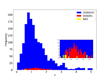
Figure 1: The redshift distribution of the QSO and BAO measurements and its details (lower right). Blue, red and yellow histograms stand for the redshift distribution of QSO[XUV], QSO[AS], and BAO respectively.

3 COSMOLOGICAL MODELS

In this paper, we concentrate on four non-standard cosmological models in a spatially flat universe, including the DGP model, Generalized Chaplygin Gas (GCG) model, the MPC model, and the power-law $f(T)$ model, based on Teleparallel Gravity.

3.1 Dvali-Gabadadze-Porrati model

Arising from the braneworld theory, the Dvali-Gabadadze-Porrati model (Dvali et al., 2000) modifies the gravity to reproduce the cosmic acceleration without need to invoke DE. In this model, we are living on a 4D membrane in a higher-dimensional spacetime. Moreover, the gravity leaks out into the bulk at large scales, which will result in the accelerated expansion of the Universe (Li et al., 2013). The Friedman equation is modified as

$$H^{2}-\frac{H}{r_{c}}=\frac{8\pi G}{3}\rho_{m},$$ (1)

where $r_{c}=1/[H_{0}(1-\Omega_{m})]$ represents the length scale beyond which the leaking occurs. We can directly rewrite the above equation and get the expansion rate

$$\frac{H(z)^{2}}{H_{0}^{2}}=\left(\sqrt{\Omega_{m}(1+z)^{3}+\Omega_{rc}}+\sqrt{\Omega_{rc}}\right)^{2},$$ (2)

where $H_{0}$ is the Hubble constant and $\Omega_{rc}=1/(4r_{c}^{2}H_{0}^{2})$ is related to the cosmological scale. Setting $z=0$ in Eq. (2), the normalization condition can be obtained

$$\Omega_{rc}=\frac{(1-\Omega_{m})^{2}}{4}.$$ (3)

and there are two free parameters ${\hat{p}}=(\Omega_{m},H_{0})$ to be constrained.

3.2 Generalized Chaplygin Gas model

As one of the candidates for dark energy models, the Chaplygin gas model, where dark energy and dark matter are unified through an exotic equation of state, has been proposed to explain the cosmic acceleration Kamenshchik et al. (2001); Bento et al. (2002); Biesiada et al. (2005); Malekjani et al. (2011). In this model, the universe is filled with the so-called Chaplygin gas, which is a perfect fluid characterized by the equation of state $p=-A/\rho$. A more general case, in which

$$p=-\frac{A}{\rho^{\alpha}},$$ (4)

where $A$ is a positive constant and $\rho$ is the energy density of this fluid, is called the generalized Chaplygin gas. The GCG model with $\alpha=0$ reduces to standard $\Lambda$CDM model and with $\alpha=1$ reduces to the standard Chaplygin gas (SCG) model. In the framework of FLRW metric, applying Eq. (4) and the conservation equation $d(\rho a^{3})=-pd(a^{3})$, the energy density of GCG model is written as

$$\rho_{GCG}=\rho_{0GCG}\left[A_{s}+(1-A_{s})a^{-3(1+\alpha)}\right]^{\frac{1}{1+\alpha}},$$ (5)

where $a$ is the scale factor, $A_{s}=A/\rho_{0GCG}^{1+\alpha}$ and $\rho_{0GCG}$ is the present energy density of the GCG. Using Eq. (4) and Eq. (5), one obtains the equation of state parameter of GCG model

$$\omega_{GCG}=-\frac{A_{s}a^{3(1+\alpha)}}{1-A_{s}+A_{s}a^{3(1+\alpha)}}.$$ (6)

Eq. (6) shows clearly that GCG acts like dust matter ($\omega_{GCG}\rightarrow 0$) in the early time ($a\rightarrow 0$) and behaves like a cosmological constant ($\omega_{GCG}\rightarrow-1$) at late epoch ($a\rightarrow\infty$). The Friedman equation for this model can be expressed as

$$\begin{split}H(z)^{2}/H_{0}^{2}=&\Omega_{b}(1+z)^{3}+\\ &(1-\Omega_{b})\left[A_{s}+(1-A_{s})(1+z)^{3(1+\alpha)}\right]^{\frac{1}{1+\alpha}},\end{split}$$ (7)

where $\Omega_{b}$ is the present density parameter of the baryonic matter. We adopt $100\Omega_{b}h^{2}=2.166\pm 0.015\pm 0.011$ with $h=H_{0}/100$ as usual and in the uncertainty budget first term is associated with the deuterium abundance measurement and the second one – with the Big Bang Nucleosynthesis (BBN) calculation used to get $\Omega_{b0}$ (Cooke et al., 2018). Since the parameter $A_{s}$ can be expressed by the effective total matter density $\Omega_{m}$ and the $\alpha$ parameter

$$A_{s}=1-\left(\frac{\Omega_{m}-\Omega_{b}}{1-\Omega_{b}}\right)^{1+\alpha},$$ (8)

there are three free parameters ${\hat{p}}=(\Omega_{m},\alpha,H_{0})$ in this model.

3.3 Power-law f(T) model

Lately, another kind of modified gravity theory-$f(T)$ (Bengochea et al., 2009; Cai et al., 2016; Qi et al., 2017) proposed in the framework of the Teleparallel Equivalent of General Relativity, has attracted a lot of attention. In this scenario, the Weitzenböck connection with torsion is used instead of torsionless Levi-Civita connection with curvature used in General Relativity. The Lagrangian density is a function $f(T)$ of the torsion scalar $T$, which is responsible for the cosmic acceleration. In this framework, the Friedman equation could be expressed as

$$\frac{H(z)^{2}}{H_{0}^{2}}=\Omega_{m}(1+z)^{3}+\Omega_{F}y(z,P),$$ (9)

where $\Omega_{F}=1-\Omega_{m}$ and $y(z,{\hat{p}})$ can be written as

$$y(z,{\hat{p}})=\frac{1}{T_{0}\Omega_{F}}(f-2Tf_{T}),$$ (10)

with $T_{0}=-6H_{0}^{2}$, $f_{T}\equiv df/dT$, and ${\hat{p}}$ representing the parameters occurring in different forms of $f(T)$ theory. In this paper, we focus on the power-law $f(T)$ model with the following form

$$f(T)=\alpha(-T)^{{}^{b}},$$ (11)

where $\alpha$ and $b$ are two model parameters. The distortion parameter $b$ quantifies the deviation from the $\Lambda$CDM model, while the parameter $\alpha$ can be expressed through the Hubble constant and density parameter $\Omega_{F0}$ by combining Eq. (9) and Eq. (11) with the boundary condition $H(z=0)/H_{0}=1$:

$$\alpha=(6H_{0}^{2})^{1-b}\frac{\Omega_{F0}}{2b-1}.$$ (12)

Now, Eq. (10) can be rewritten as

$$y(z,{\hat{p}})=E^{2b}(z,b).$$ (13)

Here we consider the Taylor expansion up to second order for Eq. (9), on $H(z,b)^{2}/H_{0}^{2}$ around $b=0$, to calculate the Friedman equation (details can be found in Nesseris et al. (2013)). Eventually, the free parameters in this $f(T)$ model are ${\hat{p}}=(\Omega_{m},b,H_{0})$.

3.4 Modified Polytropic Cardassian model

In order to explain the accelerated cosmological expansion from a different perspective, Freese et al. (2002) introduced the original Cardassian model motivated by the braneworld theory, without DE involved. In this model the Friedman equation is modified to

$$H^{2}=\frac{8\pi G\rho_{m}}{3}+B\rho_{m}^{n},$$ (14)

where $\rho_{m}$ is the total matter density and the second term on the right-hand side represents the Cardassian term. It is worth noting that the universe is driven to accelerate by the Cardassian term when the parameter $n$ satisfies $n<2/3$. Then, a simple generalized case of the Cardassian model was proposed by Gondolo et al. (2002); Wang et al. (2003), where an additional exponent $q$ was introduced. We can write the Friedman equation with this generalization as

$$\frac{H(z)^{2}}{H_{0}^{2}}=\Omega_{m}(1+z)^{3}\times\left[1+\left(\left(\frac{1}{\Omega_{m}}\right)^{q}-1\right)(1+z)^{3q(n-1)}\right]^{1/q}.$$ (15)

The MPC model, with the free parameters of ${\hat{p}}=(\Omega_{m},n,q,H_{0})$ in this model, will reduce to $\Lambda$CDM model when $q=1$ and $n=0$.

4 METHODS

In this section, we present the details of deriving observational constraints on the cosmological models from QSOs and BAO measurements.

4.1 Quasars measurements

Over the decades, a non-linear relation between the UV and X-ray luminosities of quasars have been recognized and refined (Risaliti & Lusso, 2015). This relation can be expressed as

$$\log(L_{X})=\gamma\log(L_{UV})+\beta,$$ (16)

where $\log=\log_{10}$ and the slope – $\gamma$ along with the intercept – $\beta$ are two free parameters, which should be constrained by the measurements. Applying the flux-luminosity relation of $F=L/{4\pi D_{L}^{2}}$, the UV and X-ray luminosities can be replaced by the observed fluxes:

$$\log(F_{X})=\gamma\log(F_{UV})+2(\gamma-1)\log(D_{L})+(\gamma-1)\log(4\pi)+\beta,$$ (17)

where $F_{X}$ and $F_{UV}$ are the X-ray and UV fluxes, respectively. Here $D_{L}$ is the luminosity distance, which indicates such kind of QSO measurements can be used to calibrate them as standard candles. Theoretically, $D_{L}$ is determined by the redshift $z$ and cosmological parameters ${\hat{p}}$ in a specific model:

$$D_{L}(z,{\hat{p}})=\frac{c(1+z)}{H_{0}}\int_{0}^{z}\frac{dz^{\prime}}{E(z^{\prime})},$$ (18)

where $E(z)\equiv H(z)/H_{0}$. In order to constrain cosmological parameters ${\hat{p}}$ through the measurements of QSO X-ray and UV fluxes, we compare the observed X-ray fluxes with the predicted X-ray fluxes calculated with Eq. (17) at the same redshift. Then, the best-fitted parameter values and respective uncertainties for each cosmological model are determined by minimizing the $\chi^{2}=-2\ln(LF)$ objective function, defined by the log-likelihood (Risaliti & Lusso, 2015):

$$\ln(LF)=-\frac{1}{2}\sum_{i=1}^{1598}\left[\frac{[\log(F_{X,i}^{obs})-\log(F_{X,i}^{th})]^{2}}{s_{i}^{2}}+ln(2\pi s_{i}^{2})\right],$$ (19)

where $\ln=\log_{e}$, $s_{i}^{2}=\sigma_{i}^{2}+\delta^{2}$, and In $\sigma_{i}$ is the measurement error on $F_{X,i}^{obs}$. In addition to the cosmological model parameters, three more free parameters are fitted: $\gamma$, $\beta$ representing the X-UV relation and $\delta$ representing the global intrinsic dispersion. Then, according to (Khadka et al., 2020b), for the purpose of model comparison we use the value of

$$\chi_{XUV,min}^{2}=-2\ln(LF)_{min}-\sum_{i=1}^{1598}\ln(2\pi(\sigma_{i,XUV}^{2}+\delta_{best\;fit}^{2})).$$ (20)

In our analysis, another QSO data set comes from a new compiled sample of 120 intermediate luminosity quasars (Cao et al., 2017a, b) covering the redshift range $0.46<z<2.76$ with angular sizes $\theta_{obs}(z)$, while the intrinsic length of this standard ruler is calibrated to $l_{m}=11.03\pm 0.25$ pc through a new cosmology-independent calibration technique (Cao et al., 2017b). The corresponding theoretical predictions for the angular sizes at redshift $z$ can be expressed as

$$\theta_{th}(z)=\frac{l_{m}}{D_{A}(z)},$$ (21)

where $D_{A}(z)$ is the angular diameter distance at redshift $z$ and

$$D_{A}(z)=\frac{D_{L}(z)}{(1+z)^{2}}.$$ (22)

Then, one can derive model parameters by minimizing the $\chi^{2}$ objective function:

$$\chi_{AS}^{2}(z;{\hat{p}})=\sum_{i=1}^{120}\frac{\left[\theta_{th}(z_{i};{\hat{p}})-\theta_{obs}(z_{i})\right]^{2}}{\sigma_{\theta}(z_{i})^{2}},$$ (23)

where ${\hat{p}}$ denote free parameters in a specific cosmological model and $\theta_{th}(z_{i};{\hat{p}})$ represents the theoretical value of angular sizes at redshift $z_{i}$. Moreover, an additional $10\%$ systematical uncertainty is added in the total uncertainty $\sigma_{\theta}(z_{i})^{2}$ to account for the intrinsic spread in the linear size (Cao et al., 2017b). Therefore, in our analysis, the total uncertainty is written as $\sigma_{\theta}(z_{i})^{2}=\sigma_{\theta,stat}(z_{i})^{2}+\sigma_{\theta,sys}(z_{i})^{2}$, where $\sigma_{\theta,stat}(z_{i})^{2}$ is the statistical uncertainty of $\theta_{obs}(z_{i})$ measurements.

4.2 Baryon Acoustic Oscillations measurements

For inclusion of the BAO measurements to the determination of cosmological parameters, we follow the approach carried out in Ryan et al. (2019). It is well known that the BAO data, in particular those listed in Table 1, are scaled by the size of the sound horizon at the drag epoch $r_{s}$, which can be expressed as (details can be found in Eisenstein et al. (1998))

$$r_{s}=\frac{2}{3k_{eq}}\sqrt{\frac{6}{R_{eq}}}\ln\left[\frac{\sqrt{1+R_{d}}+\sqrt{R_{d}+R_{eq}}}{1+\sqrt{R_{eq}}}\right],$$ (24)

where $R_{d}$ and $R_{eq}$ are the values of the baryon to photon density ratio

$$R=\frac{3\rho_{b}}{4\rho_{\gamma}},$$ (25)

at the drag and matter-radiation equality redshifts $z_{d}$ and $z_{eq}$, respectively, and $k_{eq}$ is the particle horizon wavenumber at $z_{eq}$. The detailed expression of $z_{d}$, $z_{eq}$, $k_{eq}$ and the baryon to photon density radio $R$ can be found in Eisenstein et al. (1998).

The BAO measurements listed in Table 1 involve the transverse comoving distance (equal to the line of sight comoving distance if $\Omega_{k0}=0$ )

$$D_{M}(z)=D_{c}(z)=\frac{c}{H_{0}}\int_{0}^{z}\frac{d{z}^{\prime}}{E({z}^{\prime})}$$ (26)

the expansion rate $H(z)$, angular diameter distance $D_{A}(z)=\frac{D_{M}(z)}{1+z}$ and the volume-averaged angular diameter distance

$$D_{V}(z)=\left[\frac{cz}{H_{0}}\frac{D_{M}^{2}(z)}{E(z)}\right]^{1/3}.$$ (27)

For the measurements of the sound horizon ($r_{s}$) scaled by its fiducial value, we use Eq. (24) to calculate both $r_{s}$ and $r_{s,fid}$, following the approach applied in Ryan et al. (2019). The parameters of $(\Omega_{m},H_{0},\Omega_{b}h^{2})$ in the fiducial cosmology are used as input to compute $r_{s,fid}$ where the BAO measurements are reported. For the analysis that scales the BAO measurements only by $r_{s}$, we turn to the fitting formula of Eisenstein et al. (1998), which is modified with a multiplicative scaling factor of 147.60 Mpc$/r_{s,Planck}$ According to the analysis of Ryan et al. (2019), such modifications to the output of the fitting formula may result in precise determinations of the size of the sound horizon $r_{s}$ and $r_{s,fid}$. Let us note that the baryon density $\Omega_{b}h^{2}$ is required to calculate the sound horizon $r_{s}$ in Eq. (24). For the uncorrelated BAO measurements listed in Table 1 (i.e. lines 7-9), the $\chi^{2}$ objective function can be written as

$$\chi_{BAO}^{2}({\hat{p}})=\sum_{i=1}^{3}\frac{\left[A_{th}(z_{i};{\hat{p}})-A_{obs}(z_{i})\right]^{2}}{\sigma(z_{i})^{2}},$$ (28)

where $A_{th}$ and $A_{obs}$ are the predicted and measured quantities of the BAO data listed in Table 1, and $\sigma(z_{i})$ stands for the relevant uncertainty of $A_{obs}$.

The BAO measurements listed in the first six lines and the last two lines of Table 1 are correlated and consequently the $\chi^{2}$ objective function takes the form

$$\chi_{BAO}^{2}({\hat{p}})=\left[A_{th}({\hat{p}})-A_{obs}\right]^{T}C^{-1}\left[A_{th}({\hat{p}})-A_{obs}\right],$$ (29)

where $C^{-1}$ denotes the inverse covariance matrix (Ryan et al., 2019)) for the BAO data taken from Alam et al. (2017), while the covariance matrix is presented in Cao et al. (2020) for the BAO data taken from de Sainte Agathe et al. (2019).

4.3 JOINT ANALYSIS

We will perform the joint analysis of the above described data to determine constraints on the parameters of a given model. In this section we outline the underlying methodology. Using the $\chi^{2}$ objective function defined above, one can write the likelihood function as

$$\mathcal{L}({\hat{p}})=e^{-\frac{\chi({\hat{p}})^{2}}{2}},$$ (30)

where ${\hat{p}}$ is the set of model parameters under consideration. Then, the likelihood function of the above combined analysis is expressed as

$$\mathcal{L}=\mathcal{L}_{XUV}\mathcal{L}_{AS}\mathcal{L}_{BAO}.$$ (31)

The likelihood analysis is performed using the Markov chain Monte Carlo (MCMC) method, implemented in the emcee package in Python 3.7 (Foreman-Mackey et al., 2013).

After constraining the parameters of each model, it is essential to determine which model is most preferred by the observational measurements and carry out a good comparison between the different models. Out of possible model selection techniques, we will use the Akaike Information Criterion (AIC) (Akaike, 1974)

$$AIC=\chi_{min}^{2}+2k,$$ (32)

as well as the Bayesian Information Criterion (BIC) (Schwarz, 1978)

$$BIC=\chi_{min}^{2}+klnN,$$ (33)

where $\chi_{min}^{2}=-2ln\mathcal{L}_{max}$, $k$ is the number of free parameters in the model and $N$ represents the number of data points. Moreover, the ratio of $\chi_{min}$ to the number of degrees of freedom $dof=N-k$, is reported as an estimate of the quality of the observational data set. The Akaike weights $\omega_{i}(AIC)$ and Bayesian weights $\omega_{i}(BIC)$ are computed through the normalized relative model likelihoods, which are expressed as

$$\omega_{i}(IC)=\frac{exp\left\{-\frac{1}{2}\Delta_{i}(IC)\right\}}{\sum_{k=1}^{K}exp\left\{-\frac{1}{2}\Delta_{k}(IC)\right\}},$$ (34)

where $\Delta_{i}(IC)$ is the difference of the value of given information criterion IC (AIC or BIC) between the model $i$ and the one which has the lowest IC and K denotes the total number of the models considered. One can find the details of the rules for estimating the AIC and BIC model selection in Biesiada (2007); Lu et al. (2008).

We supplement the model comparison by calculating the Jensen-Shannon divergence (JSD) (Lin, 1991; Abbott et al., 2019) between the posterior distributions of the common parameters assessed with two different cosmological models. The JSD is a symmetrized and smoothed measure of the distance between two probability distributions $p(x)$ and $q(x)$ defined as

$$D_{JS}(p\mid q)=\frac{1}{2}\left[D_{KL}(p\mid s)+D_{KL}(q\mid s)\right],$$ (35)

where $s=1/2(p+q)$ and $D_{KL}$ is the Kullback Leibler divergence (KLD) between the distributions $p(x)$ and $q(x)$ expressed as

$$D_{KL}(p\mid q)=\int p(x)\log_{2}\left(\frac{p(x)}{q(x)}\right)dx,$$ (36)

and a smaller value of the JSD indicates that the posteriors from two models agree well (Abbott et al., 2019).

It should be pointed out that in order to compare models through the JSD, we should use the posterior distributions of parameters ${\hat{p}}$ which are the same in the models compared. Therefore, the matter density $\Omega_{m}$ and the Hubble constant $H_{0}$ are the two parameters of interest in our analysis. In addition, we will compare the models described in Sec. 3 with $\Lambda$CDM model. Concerning the posterior distributions of common free parameters in different models, they can be obtained through the MCMC method, then we take advantage of the dedicated Python 3.7 package to compute the JSD between two one-dimensional (1D) probability distributions.

model	data	$\Omega_{m}$	$\beta$	$\gamma$	$\delta$	$H_{0}$
$\Lambda$CDM	QSO[XUV]+QSO[AS]	$0.406_{-0.082}^{+0.108}$	$7.321_{-0.314}^{+0.308}$	$0.631_{-0.010}^{+0.010}$	$0.231_{-0.004}^{+0.004}$	$64.704_{-3.744}^{+3.347}$
	BAO	$0.316_{-0.020}^{+0.022}$	-	-	-	$68.074_{-1.380}^{+1.545}$
	QSO[XUV]+QSO[AS]+BAO	$0.317_{-0.007}^{+0.007}$	$7.152_{-0.260}^{+0.265}$	$0.637_{-0.009}^{+0.009}$	$0.231_{-0.004}^{+0.004}$	$68.157_{-0.487}^{+0.496}$
model	data	$\Omega_{m}$	$\beta$	$\gamma$	$\delta$	$H_{0}$
DGP	QSO[XUV]+QSO[AS]	$0.365_{-0.100}^{+0.129}$	$7.358_{-0.309}^{+0.328}$	$0.630_{-0.010}^{+0.010}$	$0.231_{-0.004}^{+0.004}$	$62.353_{-3.709}^{+3.877}$
	BAO	$0.269_{-0.020}^{+0.022}$	-	-	-	$59.560_{-1.004}^{+1.149}$
	QSO[XUV]+QSO[AS]+BAO	$0.329_{-0.009}^{+0.009}$	$7.299_{-0.271}^{+0.263}$	$0.632_{-0.009}^{+0.009}$	$0.231_{-0.004}^{+0.004}$	$62.757_{-0.471}^{+0.488}$
model	data	$\Omega_{m}$	$\alpha$	$\beta$	$\gamma$	$\delta$	$H_{0}$
GCG	QSO[XUV]+QSO[AS]	$0.416_{-0.068}^{+0.088}$	$2.360_{-1.793}^{+1.803}$	$7.419_{-0.340}^{+0.326}$	$0.628_{-0.011}^{+0.011}$	$0.231_{-0.004}^{+0.004}$	$69.254_{-4.970}^{+4.427}$
	BAO	$0.299_{-0.039}^{+0.029}$	$-0.227_{-0.246}^{+0.272}$	-	-	-	$63.972_{-5.866}^{+5.266}$
	QSO[XUV]+QSO[AS]+BAO	$0.319_{-0.009}^{+0.010}$	$-0.067_{-0.147}^{+0.151}$	$7.186_{-0.250}^{+0.259}$	$0.636_{-0.009}^{+0.008}$	$0.231_{-0.004}^{+0.005}$	$67.496_{-1.904}^{+1.605}$
model	data	$\Omega_{m}$	$b$	$\beta$	$\gamma$	$\delta$	$H_{0}$
f(T)	QSO[XUV]+QSO[AS]	$0.409_{-0.090}^{+0.131}$	$-0.193_{-0.509}^{+0.551}$	$7.344_{-0.331}^{+0.313}$	$0.631_{-0.010}^{+0.011}$	$0.231_{-0.005}^{+0.005}$	$63.829_{-4.839}^{+4.147}$
	BAO	$0.303_{-0.029}^{+0.028}$	$0.261_{-0.323}^{+0.252}$	-	-	-	$64.154_{-4.858}^{+4.806}$
	QSO[XUV]+QSO[AS]+BAO	$0.320_{-0.009}^{+0.010}$	$0.084_{-0.166}^{+0.176}$	$7.163_{-0.269}^{+0.280}$	$0.637_{-0.009}^{+0.009}$	$0.231_{-0.004}^{+0.005}$	$67.507_{-1.987}^{+1.327}$
model	data	$\Omega_{m}$	$q$	$n$	$\beta$	$\gamma$	$\delta$	$H_{0}$
MPC	QSO[XUV]+QSO[AS]	$0.410_{-0.062}^{+0.085}$	$1.936_{-0.982}^{+2.923}$	$-0.547_{-0.981}^{+0.564}$	$7.497_{-0.374}^{+0.343}$	$0.626_{-0.011}^{+0.012}$	$0.231_{-0.004}^{+0.005}$	$70.576_{-4.435}^{+6.475}$
	BAO	$0.304_{-0.034}^{+0.030}$	$0.914_{-0.322}^{+0.381}$	$0.120_{-0.320}^{+0.192}$	-	-	-	$63.800_{-5.620}^{+5.177}$
	QSO[XUV]+QSO[AS]+BAO	$0.321_{-0.011}^{+0.011}$	$0.944_{-0.183}^{+0.237}$	$0.022_{-0.205}^{+0.165}$	$7.176_{-0.253}^{+0.290}$	$0.636_{-0.010}^{+0.008}$	$0.231_{-0.005}^{+0.005}$	$67.462_{-2.324}^{+1.663}$

Table 2: Summary of the best-fit values with their 1$\sigma$ uncertainties concerning the parameters of all considered models. The results are obtained from the combined data sets of QSO[XUV]+QSO[AS], BAO and QSO[XUV]+QSO[AS]+BAO.

data	model	AIC	$\Delta$AIC	$\omega_{i}(AIC)$	BIC	$\Delta$BIC	$\omega_{i}(BIC)$	$\chi_{min}^{2}/dof$	$D_{JS}(\Omega_{m})$	$D_{JS}(H_{0})$
QSO[XUV]+QSO[AS]	$\Lambda$CDM	2217.95	1.25	0.257	2245.19	1.25	0.3419	1.289	0	0
	DGP	2216.70	0	0.479	2243.94	0	0.6376	1.288	0.233	0.273
	GCG	2218.58	1.88	0.188	2251.27	7.32	0.0164	1.289	0.199	0.447
	f(T)	2221.43	4.73	0.045	2254.12	10.18	0.0039	1.291	0.161	0.136
	MPC	2222.20	7.38	0.031	2260.34	16.40	0.0002	1.291	0.224	0.516
BAO	$\Lambda$CDM	13.88	1.57	0.233	14.68	1.57	0.2454	1.098	0	0
	DGP	12.32	0	0.511	13.11	0	0.5370	0.924	0.749	0.999
	GCG	15.95	3.63	0.083	17.14	4.03	0.0716	1.244	0.339	0.658
	f(T)	14.71	2.39	0.155	15.90	2.79	0.1332	1.090	0.270	0.640
	MPC	18.99	1.57	0.018	20.59	7.47	0.0128	1.571	0.255	0.663
QSO[XUV]+QSO[AS]+BAO	$\Lambda$CDM	2227.20	0	0.780	2254.47	0	0.9483	1.286	0	0
	DGP	2233.63	6.43	0.031	2260.90	6.43	0.0381	1.289	0.566	0.999
	GCG	2230.45	3.25	0.153	2263.18	8.71	0.0122	1.288	0.198	0.586
	f(T)	2234.92	7.72	0.016	2267.65	13.18	0.0013	1.290	0.214	0.547
	MPC	2234.58	7.38	0.020	2272.77	18.30	0.0001	1.290	0.322	0.629

Table 3: Information theoretic model comparison. Minimum values of AIC, BIC, their differences and weights are reported for the $\Lambda$CDM and each of the four cosmological models considered. Jensen-Shannon divergence $D_{JS}$ between $\Lambda$CDM and other cosmological models was calculated with respect to the matter density parameter $\Omega_{m}$ and the Hubble constant $H_{0}$.

5 RESULTS AND DISCUSSION

In this section, we present the results for the four cosmological models listed in Sec. 3, obtained using different combination of data sets: QSO[XUV]+QSO[AS], BAO and QSO[XUV]+QSO[AS]+BAO. In order to have a good comparison, the corresponding results for the concordance $\Lambda$CDM model is also displayed. The 1D probability distributions and 2D contours with $1\sigma$ and $2\sigma$ confidence levels, as well as the best-fit value with 1 $\sigma$ uncertainty for each model are shown in Figs. 2-6 and reported in Table 2.

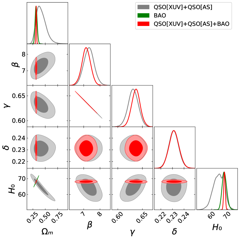
Figure 2: The 1D probability distributions and 2D contours with $1\sigma$ and $2\sigma$ confidence levels for $\Lambda$CDM model obtained from QSO[XUV]+QSO[AS] (gray), BAO (green) and QSO[XUV]+QSO[AS]+BAO (red) data.

5.1 Observational Constraints on Dvali-Gabadadze-Porrati model

As can be seen from Fig. 3, the combined QSO measurements (QSO[XUV]+QSO[AS]) do not provide stringent constraints on the matter density parameter $\Omega_{m}$, which will be improved with the combination of recent BAO observations. The best-fit value of $\Omega_{m}$ given by QSO[XUV]+QSO[AS] is $\Omega_{m}=0.365_{-0.100}^{+0.129}$ within 68.3% confidence level, which agrees well with the QSO[AS] data alone: $\Omega_{m}=0.285_{-0.155}^{+0.255}$ (without systematics) (Cao et al., 2017b), the recent Planck 2018 results: $\Omega_{m}=0.315\pm 0.007$ (Planck Collaboration et al., 2018) and SNe Ia+BAO+CMB+observational Hubble parameter (OHD): $\Omega_{m}=0.305\pm 0.015$ (Shi et al., 2012). However, it is worthwhile to mention that the matter density parameter $\Omega_{m}$ obtained by QSO tends to be higher than that from other cosmological probes, as was remarked in the previous works of Risaliti & Lusso (2019); Khadka et al. (2020b). This suggests that the composition of the universe characterized by cosmological parameters can be comprehended differently through high-redshift quasars. For the BAO data, the best-fit matter density parameter is $\Omega_{m}=0.269_{-0.020}^{+0.022}$, which is significantly lower than that from the modified gravity theories considered in this paper. Interestingly, the estimated values of $\Omega_{m}$ are in agreement with the standard ones reported by other astrophysical probes, such as $\Omega_{m}=0.277_{-0.017}^{+0.017}$ given by the linear growth factors combined with CMB+BAO+SNe+GRB observations (Xia et al., 2009), $\Omega_{m}=0.235_{-0.074}^{+0.125}$ given by galaxy clusters combined with SNe+GRBs+CMB+BAO+OHD observations (Liang et al., 2011), and $\Omega_{m}=0.243_{-0.074}^{+0.077}$ given by strong gravitational lensing systems (Ma et al., 2019). For comparison, the fitting results from the combined QSO[XUV]+QSO[AS]+BAO data sets are also shown in Fig. 3, with the the matter density parameter of $\Omega_{m}=0.329_{-0.009}^{+0.009}$. The use of BAO data to constrain cosmological models seems to be complementary to the QSO distance measurements, considering the constrained results especially on $\Omega_{m}$ and $H_{0}$.

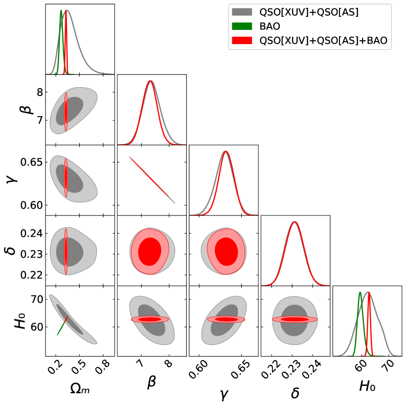
Figure 3: The 1D probability distributions and 2D contours with $1\sigma$ and $2\sigma$ confidence levels for DGP model obtained from QSO[XUV]+QSO[AS] (gray), BAO (green) and QSO[XUV]+QSO[AS]+BAO (red) data.

5.2 Observational Constraints on Generalized Chaplygin Gas model

Fig. 4 and Table 2 present the results of the best-fitted parameters for the GCG model. One can see a deviation between the constraints of ($\Omega_{m}$, $\alpha$, $H_{0}$) coming from the three combined data sets, which are still consistent with each other within $2\sigma$ confidence level. On the one hand, the combined data sets QSO[XUV]+QSO[AS] can not tightly constrain the model parameters ($\Omega_{m}$,$\alpha$), especially for parameter $\alpha$ whose best-fit value is $\alpha=2.360_{-1.793}^{+1.803}$ and $\Omega_{m}$ is much larger than the value implied by other measurements. In the framework of GCG, considering the fact that the parameter $\alpha$ quantifies the deviation from the $\Lambda$CDM model and the SCG model, $\Lambda$CDM is not consistent with GCG at $1\sigma$ confidence level, while SCG is more favored by the QSO[XUV]+QSO[AS] data. However, in the case of BAO and QSO[XUV]+QSO[AS]+BAO data, $\Lambda$CDM is still favored within $1\sigma$, with $\alpha=-0.227_{-0.246}^{+0.272}$ and $\alpha=-0.067_{-0.147}^{+0.151}$ respectively. The combined data set of QSO[XUV]+QSO[AS]+BAO provides more stringent constraints on the matter density parameter ($\Omega_{m}=0.319_{-0.009}^{+0.010}$) and the Hubble constant ($H_{0}=67.496_{-1.904}^{+1.605}\mathrm{~{}km~{}s^{-1}~{}Mpc^{-1}}$). For comparison, the results obtained from the joint light-curve analysis (JLA) compilation of SNe Ia, CMB, BAO, and 30 OHD data simulated over redshift range $2\leqslant z\leqslant 5$ gave $\Omega_{m}=0.345_{-0.006}^{+0.006}$ and $\alpha=-0.047_{-0.026}^{+0.027}$ (Liu et al., 2019), which prefers a higher value of $\Omega_{m}$ than our results and does not include $\Lambda$CDM within $1\sigma$ range. It is interesting to note that Liu et al. (2019) also obtained $\alpha=-0.040_{-0.065}^{+0.060}$ without adding the simulated data, which still includes the $\Lambda$CDM model at $1\sigma$ confidence level and is slightly different from the results obtained by adding the simulated higher redshift. This may indicate that the data within the “redshift desert” ($2\leqslant z\leqslant 5$) can provide a valuable supplement to other astrophysical observations in the framework of GCG model.

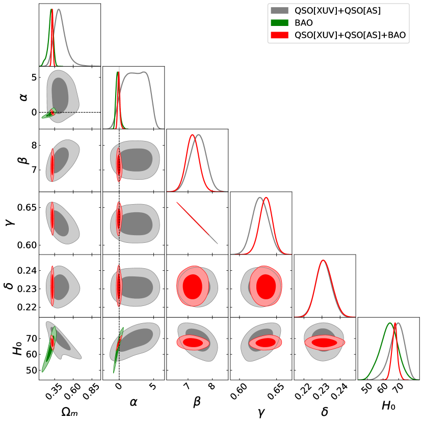
Figure 4: The 1D probability distributions and 2D contours with $1\sigma$ and $2\sigma$ confidence levels for GCG model obtained from QSO[XUV]+QSO[AS] (gray), BAO (green) and QSO[XUV]+QSO[AS]+BAO (red) data. The black dashed line represents the $\Lambda$CDM model corresponding to $\alpha=0$.

5.3 Observational Constraints on Power-law F(T) model

In the case of $f(T)$ theory based on $f(T)=\alpha(-T)^{{}^{b}}$ ansatz, the results are presented in Fig. 5 and can be seen in Table 2. It can be clearly seen from the comparison plots, there is a consistency between QSO[XUV]+QSO[AS], BAO and QSO[XUV]+QSO[AS]+BAO. However, the QSO[XUV]+QSO[AS] data generate a higher matter density parameter $\Omega_{m}=0.409_{-0.090}^{+0.131}$ compared with other probes. As for the parameter $b$ which captures the deviation of the $f(T)$ model from the $\Lambda$CDM model, the best-fit value is $b=-0.193_{-0.509}^{+0.551}$ and the $\Lambda$CDM model ($b=0$) is still included within $1\sigma$ range. Such conclusion could also be carefully derived in the case of BAO and QSO[XUV]+QSO[AS]+BAO measurements. For comparison, our results are similar to the results obtained with QSO(AS)+SNe Ia+BAO+CMB data sets ($\Omega_{m}=0.317\pm 0.010$, $b=0.057_{-0.065}^{+0.091}$) (Qi et al., 2017) and SNe Ia+BAO+CMB+dynamical growth data ($\Omega_{m}=0.272\pm 0.008$, $b=-0.017\pm 0.083$) (Nesseris et al., 2013), where the value of $\Omega_{m}$ is in tension with our results within $1\sigma$. Moreover, in the framework of the power-law $f(T)$ model, the parameter $b$ obtained from QSO[XUV]+QSO[AS] and BAO alone seems to deviate from zero more according to the above mentioned results, which suggests that there are still some possibility that $\Lambda$CDM may not be the best cosmological model preferred by current observations with larger redshift range. With the combined data sets QSO[XUV]+QSO[AS]+BAO, we also get stringent constraints on the model parameters $\Omega_{m}=0.320_{-0.010}^{+0.009}$, $b=0.084_{-0.166}^{+0.176}$ and $H_{0}=67.507_{-1.987}^{+1.327}\mathrm{~{}km~{}s^{-1}~{}Mpc^{-1}}$, where $\Lambda$CDM is included within $1\sigma$. It is worth noting that this slight deviation from the $\Lambda$CDM is also in agreement with similar results in the literature, obtained from QSO[AS]+BAO+CMB ($b=0.080\pm 0.077$) (Qi et al., 2017) and OHD+SN Ia+BAO+CMB ($b=0.05128_{-0.019}^{+0.025}$) (Nunes et al., 2016).

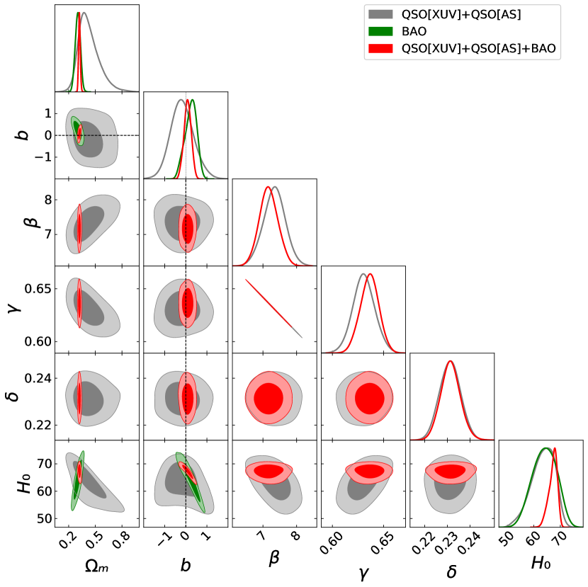
Figure 5: The 1D probability distributions and 2D contours with $1\sigma$ and $2\sigma$ confidence levels for $f(T)$ model obtained from QSO[XUV]+QSO[AS] (gray), BAO (green) and QSO[XUV]+QSO[AS]+BAO (red) data. The black dashed line represents the $\Lambda$CDM model corresponding to $b=0$.

5.4 Observational Constraints on Modified Polytropic Cardassian model

All values of the estimated cosmic parameters in the MPC model are displayed in Table 2 and illustrated in Fig. 6. For the QSO[XUV]+QSO[AS], BAO and QSO[XUV]+QSO[AS]+BAO data, the best-fit values of the parameters ($q$ and $n$) are in good agreement with each other within within $2\sigma$. Meanwhile, $\Lambda$CDM is still favored by the current QSO and BAO measurements within $1\sigma$ confidence level in the MPC model. Apparently, however, the combined QSO data supports higher matter density parameter $\Omega_{m}=0.410_{-0.062}^{+0.085}$ than that from the other two data sets within 68.3% confidence level. The constraints on the parameters $q$ and $n$ from the QSO[XUV]+QSO[AS] data are very weak: $q=1.936_{-0.982}^{+2.923}$, $n=-0.547_{-0.981}^{+0.564}$, but it seems that the central values of $q$ and $n$ deviate more from 1 and 0, respectively in comparison to the results obtained with BAO and QSO[XUV]+QSO[AS]+BAO. This may suggest, that the quasar data (especially QSO[XUV]) at higher redshift may have some possibility of favoring the modifications to the Friedmann equations in the MPC model. Several authors have tested the MPC model with different measurements. For instance, the SNe Ia+BAO+CMB+OHD data sets gave $q=0.897_{-0.468}^{+0.152}$, $n=-0.648_{-1.106}^{+0.856}$ (Shi et al., 2012), which are in good accordance with our results obtained of the BAO measurements and QSO[XUV]+QSO[AS]+BAO. In addition, our limits are similar to $q=3.29\pm 3.30$, $n=0.26\pm 0.13$ shown in Magana et al. (2015) using BAO data, and in tension with the results obtained from strong lensing measurements (Magana et al., 2015) in Abell1689: $q=5.2\pm 2.25$, $n=0.41\pm 0.25$. With the SNLS3 SN Ia sample+CMB+BAO+OHD data sets, Li et al. (2012) got the constraints $q=1.098_{-0.465}^{+1.015}$ and $n=0.014_{-0.946}^{+0.364}$, which is consistent with our limits. Note that, also with the QSO[XUV]+QSO[AS]+BAO data sets the best-fit values of $q$ and $n$ parameters deviate from 1 and 0 respectively, which implies the possibility of the modifications to the Friedmann equations.

From our constraints on the matter density parameter $\Omega_{m}$ in different non-standard cosmological models, one thing is quite clear, which is that the combined QSO data containing large number of measurements at high redshifts ($2\leqslant z\leqslant 5$) do favor $\Omega_{m}$ lying in the range from $0.365_{-0.100}^{+0.129}$ to $0.416_{-0.068}^{+0.088}$. This is considerably higher than the constraints from other probes (such as BAO measurements). Actually, such results on $\Omega_{m}$ have been noted in the previous works through different approaches. For instance, Khadka et al. (2020b) obtained $\Omega_{m}\sim 0.5-0.6$ in four different cosmological models with large number of QSO[XUV], while Qi et al. (2017) derived $\Omega_{m}=0.319\pm 0.011$ and $\Omega_{m}=0.329\pm 0.011$ in different $f(T)$ theories with QSO[AS]+BAO+CMB data sets. Other studies of different dark energy models (based on Pade approximation parameterizations) revealed the similar conclusions with Pantheon+GRB+QSO: the matter density parameter lies in the range from $\Omega_{m}=0.384_{-0.022}^{+0.033}$ to $\Omega_{m}=0.391_{-0.026}^{+0.038}$ (Rezaei et al., 2020). Meanwhile, some recent studies (Risaliti & Lusso, 2019; Lusso et al., 2019; Rezaei et al., 2020; Benetti et al., 2019; Yang et al., 2020; Demianski et al., 2020; Li et al., 2021) focused on exploring the deviation between high redshift measurements and the standard cosmological model. Despite of the $\Omega_{m}$ inconsistency obtained from the measurements with different redshift coverage, it is still under controversy whether this is an indication of a new physics or an unknown systematic effect of the high-redshift observations. Therefore, besides developing new high quality and independent cosmological probes, it would be more interesting to figure out why the standard cosmological parameters are fitted to different values with high and low redshift observations. The latter indicates that one could go beyond $\Lambda$CDM model to properly describe our universe (Ding et al., 2015; Zheng et al., 2016).

As for the constraints on the Hubble constant $H_{0}$ shown in Table 2, one can see that $H_{0}$ lies in the range from $H_{0}=62.353_{-3.709}^{+3.877}$ to $H_{0}=70.576_{-4.435}^{+6.475}\mathrm{~{}km~{}s^{-1}~{}Mpc^{-1}}$ for the combined QSO data, from $H_{0}=59.560_{-1.004}^{+1.149}$ to $H_{0}=68.074_{-1.380}^{+1.545}\mathrm{~{}km~{}s^{-1}~{}Mpc^{-1}}$ for BAO, and from $H_{0}=62.757_{-0.471}^{+0.488}$ to $H_{0}=68.157_{-0.487}^{+0.496}\mathrm{~{}km~{}s^{-1}~{}Mpc^{-1}}$ for QSO[XUV]+QSO[AS]+BAO. Apparently, almost all the results for $H_{0}$ are lower than $70\mathrm{~{}km~{}s^{-1}~{}Mpc^{-1}}$, except for the MPC model assessed with QSO[XUV]+QSO[AS] which however has large uncertainties.

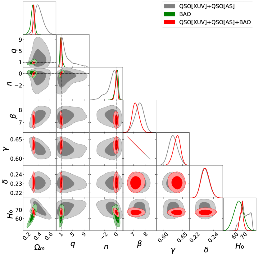
Figure 6: The 1D probability distributions and 2D contours with $1\sigma$ and $2\sigma$ confidence levels for MPC model, obtained from QSO[XUV]+QSO[AS] (gray), BAO (green) and QSO[XUV]+QSO[AS]+BAO (red) data. The black dashed line indicates the $\Lambda$CDM model corresponding to $q=1$ and $n=0$.

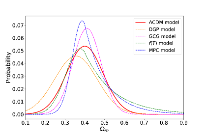
(a) Combined QSO

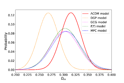
(b) BAO

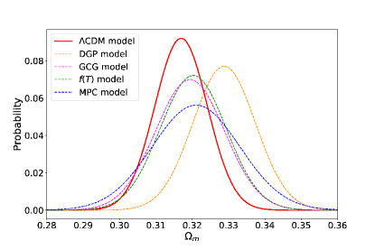
(c) Combined QSO and BAO

Figure 7: The posterior distributions of $\Omega_{m}$ for $\Lambda$CDM, DGP, GCG, $f(T)$, and MPC model, with the combined QSO, BAO and combined QSO+BAO data.

5.5 MODEL COMPARISON

In this section we compare the models and discuss how strongly are they supported by the observational data sets. In Table 3 one can find the summary of the information theoretical model selection criteria applied to different models from QSO[XUV]+QSO[AS], BAO and QSO[XUV]+QSO[AS]+BAO data sets. It can be seen that $\Lambda$CDM is still the best model for the combined data QSO[XUV]+QSO[AS]+BAO, under the assessment of AIC and BIC. Although the quasar sample (QSO[XUV]+QSO[AS]) and the BAO data tend to prefer the DGP model in term of AIC and BIC, they also share the same preference for $\Lambda$CDM, compared with other theories of modified gravity.

It is important to keep in mind that model selection provides a quantitative information on the strength of evidence (or the degree of support) rather than just selecting only one model (Lu et al., 2008). Table 3 informs us that AIC applied to the QSO[XUV]+QSO[AS] data set does not effectively discriminate $\Lambda$CDM and GCG models – both of them receive the similar support, while the evidence against $f(T)$ and MPC model is very strong. For the QSO[XUV]+QSO[AS]+BAO data, we find that the DGP, $f(T)$ and MPC model are clearly disfavored by the data, as they are unable to provide a good fit. The BIC diversifies the evidence between the models. Out of all the candidate models, it is obvious that models with more free parameters (GCG, $f(T)$ and MPC) are less favored by the current quasar observations (QSO[XUV]+QSO[AS]). Among these four modified gravity models, the evidence against MPC is very noticeable for all kinds of data sets, which demonstrates the MPC model is seriously punished by the BIC.

Traditional information criteria (AIC or BIC) do not provide much insight into the agreement between $\Lambda$CDM and the other four models. Therefore, we also calculated the JSD (see Sec. 4.4) in order to assess which models are consistent with $\Lambda$CDM in light of the observational data. As already mentioned one should have common parameters in all compared models and we used in this role the matter density parameter and Hubble constant. Figs. 7-8 show the posterior distribution of $\Omega_{m}$ and $H_{0}$ obtained with QSO[XUV]+QSO[AS], BAO and QSO[XUV]+QSO[AS]+BAO data sets for all models considered. For QSO[XUV]+QSO[AS] data, the posterior distributions of $\Omega_{m}$ and $H_{0}$ in $f(T)$ models agree more with that of $\Lambda$CDM in terms of the value of JSD. As for the BAO measurements, the value of JSD concerning $\Omega_{m}$ shows the MPC model agree more with the $\Lambda$CDM, but concerning $H_{0}$, all four non-standard models give large distance from the $\Lambda$CDM, where the $f(T)$ model is still the closest to it. In the case of QSO[XUV]+QSO[AS]+BAO data sets, the DGP and MPC model are much more distant from the $\Lambda$CDM for the posterior distributions of $\Omega_{m}$, while GCG and $f(T)$ model is closer to it, which is similar to the cases for the posterior distributions of $H_{0}$.

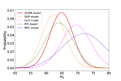
(a) Combined QSO

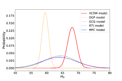
(b) BAO

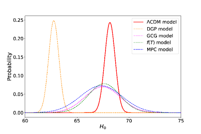
(c) Combined QSO and BAO

Figure 8: The posterior distributions of $H_{0}$ for $\Lambda$CDM, DGP, GCG, $f(T)$, and MPC model, with the combined QSO, BAO and combined QSO+BAO data.

6 CONCLUSIONS

The modified gravity could provide interesting approaches to explain the cosmic acceleration, without involving dark energy. In this paper, we have evaluated the power of multiple measurements of quasars covering sufficiently wide redshift range, on constraining some popular modified gravity theories including DGP, GCG, the power-law $f(T)$ model and MPC model, under the assumption of the spatial flatness of the Universe. As for the observational data, the newest large sample of QSO X-ray and UV flux measurements (Risaliti & Lusso, 2019) were used as standard candles and provided a good opportunity to test models at the "redshift desert" ($2\leqslant z\leqslant 5$) that is not yet widely available through other observations. In addition, a popular compilation of 120 angular size measurements of compact structure in radio quasars versus redshift data from very-long-baseline interferometry (VLBI) over the redshift range $0.46<z<2.76$ (Cao et al., 2017b) was used as standard rulers to test these models in conjunction with the 1598 QSO X-Ray and UV flux measurements. Meanwhile, with the aim to tighten the constraint from the combined QSO data sets and test the consistency with other observations, 11 recent BAO measurements in the redshift range $0.122\leq z\leq 2.34$ (Cao et al., 2020) were also taken into account in this work. Here we summarize our main conclusions in more detail:

• Our results show that calibrating parameters $\beta$ and $\gamma$ from the non-linear $L_{X}-L_{UV}$ relation, as well as the global intrinsic dispersion $\delta$ are almost independent of the cosmological model, which is similar to the results from Khadka et al. (2020b). This supports the evidence that these selected quasars can be regarded as standard candles.

• In all four non-standard cosmological models, the results show that the combined QSO data alone are not able to provide tight constraints on model parameters, which is mainly related to the large dispersion ($\delta=0.23$) of the $L_{X}-L_{UV}$ relation obtained from the 1598 QSO X-Ray and UV flux measurements. On the other hand, the combined quasar data constraints are mostly coherent with the joint analysis including BAO measurements. The value of matter density parameter $\Omega_{m}$ implied by the combined QSO data is noticeably larger than that derived from other measurements, which is likely caused by the discrepancy between the QSO X-Ray and UV flux data and the $\Omega_{m}=0.3$ flat $\Lambda$CDM (Risaliti & Lusso, 2019; Khadka et al., 2020b). It is quite possible that quasar data at high redshifts can shed new light on the model of our universe. Moreover, in this paper, we tested different alternative models. Most of them include the concordance $\Lambda$CDM model as a special case corresponding to certain values of their parameters, such as the parameter $b$ in the power-law $f(T)$ model. For the $f(T)$ and MPC model, $\Lambda$CDM turned out to be compatible with them at $1\sigma$ confidence level, while the GCG model is generally inconsistent with the cosmological constant case within $1\sigma$. Furthermore, after including BAO in the joint analysis, the best-fit value of these parameters and their $1\sigma$ confidence levels show less deviation from $\Lambda$CDM, which suggests that BAO measurements favor $\Lambda$CDM significantly.

• According to the AIC and BIC, the concordance $\Lambda$CDM model is still the best cosmological model in light of the combined QSO and BAO data, while the MPC model has considerably less support as the best one. Although the quasar sample (QSO[XUV]+QSO[AS]) and the BAO data tend to prefer the DGP model in term of AIC and BIC, they also share the same preference for $\Lambda$CDM, compared with other theories of modified gravity. Therefore, non-standard models with more free parameters are less favored by the available observations, which is the most unambiguous result of the current dataset. In order to compare the agreement between the $\Lambda$CDM model and other four models, Jensen-Shannon divergence (JSD) was applied in this paper. We found that for the combined QSO data, the posterior distribution of $\Omega_{m}$ and $H_{0}$ from $f(T)$ were in a better agreement with $\Lambda$CDM. For BAO measurements, MPC and $f(T)$ models are closer to $\Lambda$CDM according to the values of JSD from the posterior distribution of $\Omega_{m}$, while all four models are distant from $\Lambda$CDM in the case of $H_{0}$, especially the DGP model. With QSO+BAO data, the results are similar to that from BAO measurements, but the posterior distribution of $\Omega_{m}$ from GCG and $f(T)$ model are in better agreement with $\Lambda$CDM.

Data Availability Statements

The data underlying this article will be shared on reasonable request to the corresponding author.

References

- Abbott et al. (2019) Abbott, B. P., et al. 2019, PRX, 9, 031040
- Akaike (1974) Akaike, H. 1974, IEEE Trans. Autom. Control, 19, 716
- Alam et al. (2017) Alam, S., et al. 2017, MNRAS, 470, 2617
- Allen et al. (2008) Allen, S. W., Rapetti, D. A., Schmidt, R. W., Ebeling, H., Morris, R. G., Fabian, A. C. 2008, MNRAS, 383, 879
- Amante et al. (2020) Amante, M. H., et al. 2019, MNRAS, 498, 6013
- Amendola (2000) Amendola, L. 2000, PRD, 62, 043511
- Ata et al. (2018) Ata, M., et al. 2018, MNRAS, 473, 4773
- Avni & Tananbaum (1986) Avni, Y., & Tananbaum, H. 1986, ApJ, 305, 83
- Baldwin (1977) Baldwin, J. A. 1977, ApJ, 214, 679
- Bengochea et al. (2009) Bengochea, G.R., Ferraro, R. 2009, PRD, 79, 124019
- Bento et al. (2002) Bento, M. C., Bertolami, O., Sen, A. A. 2002, PRD, 66, 043507
- Biesiada et al. (2005) Biesiada, M., God lowski, W., & Szydłowski, M. 2005, ApJ, 622, 28
- Biesiada (2007) Biesiada, M. 2007, JCAP, 02, 003B
- Biesiada et al. (2011) Biesiada, M., Malec, B., & Piorkowska, A. 2011, RAA, 11, 641
- Bisogni et al. (2018) Bisogni, S., et al. 2017, Front Astron Space. Sci, 4, 68
- Boisseau et al. (2000) Boisseau, B., Esposito-Farese, G., Polarski, D., Starobinsky, A. A. 2000, PRL, 85, 2236
- Bonamente et al. (2006) Bonamente, M., et al. 2006, ApJ, 647, 25
- Benetti et al. (2019) Benetti, M., & Capozziello, S. 2019, JCAP, 1912, 008
- Cai et al. (2016) Cai, Y.-F., Capozziello, S., De Laurentis, M., Saridakis, E. N. 2016, RPPh, 79, 106901
- Caldera-Cabral et al. (2009) Caldera-Cabral, G., Maartens, R., Urena-Lopez, L. A. 2009, PRD, 79, 063518
- Caldwell et al. (2005) Caldwell, R., Linder E.V. 2005, PRL, 888, L25
- Cao et al. (2011) Cao, S., Zhu, Z.-H., & Zhao, R. 2011, PRD, 84, 023005
- Cao & Zhu (2012) Cao, S., & Zhu, Z.-H. 2012, A&A, 538, A43
- Cao, Covone & Zhu (2012) Cao, S., Covone, G., & Zhu, Z.-H. 2012, ApJ, 755, 31
- Cao et al. (2012) Cao, S., Pan, Y., Biesiada, M., Godlowski, W., & Zhu Z.-H. 2012, JCAP, 03, 016
- Cao et al. (2015b) Cao, S., Biesiada, M., Gavazzi, R., Piórkowska, A., & Zhu, Z.-H. 2015b, ApJ, 806, 185
- Cao et al. (2017a) Cao, S., et al. 2017, JCAP, 02, 012
- Cao et al. (2017b) Cao, S., et al. 2017, A&A, 606, A15
- Cao et al. (2017c) Cao, S., et al. 2017, ApJ, 835, 92
- Cao et al. (2018) Cao, S., Biesiada, M., Zheng, X. G., et al. 2018, EPJC, 78, 749
- Cao et al. (2019) Cao, S., et al. 2019, PDU, 24, 100274
- Cao et al. (2020) Cao, S., et al. 2020, ApJL, 888, L25
- Cao et al. (2020) Cao, S. L., Ryan, J., Ratra, B. 2020, MNRAS, 497, 3191
- Carter et al. (2018) Carter, P., Beutler, F., Percival, W. J., Blake, C., Koda, J., Ross, A. J. 2018, MNRAS, 481, 2371
- Chen et al. (2003) Chen, G., Ratra, B. 2003, ApJ, 582, 586
- Chen et al. (2011) Chen, Y., Ratra, B. 2011, PLB, 703, 406
- Chen et al. (2012) Chen, Y., Ratra, B. 2012, A&A, 543, A104
- Chen et al. (2015) Chen, Y., Geng, C.-Q., Cao, S., Huang, Y.-M., Zhu, Z.-H. 2015, JCAP, 2, 010
- Chen et al. (2016) Chen, Y., Ratra, B., Biesiada, M., Li, S., Zhu, Z.-H. 2016, ApJ, 829, 61
- Chiba et al. (2003) Chiba, T. 2003, PLB, 575, 1
- Clifton et al. (2012) Clifton, T., Ferreira, P. G., Padilla, A., Skordis, C. 2012, Phys. Rep., 513, 1
- Cooke et al. (2018) Cooke, R. J., Pettini, M., Steidel, C. C. 2018, ApJ, 855, 102
- Copeland et al. (2006) Copeland, E. J., Sami, M., Tsujikawa, S. 2006, IJMPD, 15, 1753
- De Bernardis et al. (2006) De Bernardis, F., Giusarma, E., Melchiorri, A. 2006, IJMPD, 15, 759
- DES Collaboration (2019) DES Collaboration 2019, MNRAS, 483, 4866
- de Sainte Agathe et al. (2019) de Sainte Agathe V. et al., 2019, A&A, 629, A85
- Ding et al. (2015) Ding, X., et al. 2015, ApJL, 803, L22
- Dvali et al. (2000) Dvali, G., Gabadadze, G., Porrati, M. 2000, PLB, 485, 208
- Demianski et al. (2020) Demianski, M., et al. 2020, Frontiers in Astronomy and Space Sciences, 7, 69
- Eisenstein et al. (1998) Eisenstein, D. J., Hu, W. 1998, ApJ, 496, 605
- Eisenstein et al. (2005) Eisenstein, D. J., et al. 2005, ApJ, 633, 560
- Farooq et al. (2017) Farooq, O., Madiyar, F., Crandall, S, Ratra, B. 2017, ApJ, 835, 26
- Foreman-Mackey et al. (2013) Foreman-Mackey, D., Hogg, D. W., Lang, D., Goodman, J. 2013, PASP, 125, 306
- Freese et al. (2002) Freese, K., Lewis, M. 2002, PLB, 540, 1
- Geng et al. (2020) Geng, S. B., Cao, S., Liu, T. H., Biesiada, M., Qi, J.-Z., Liu, Y. T., Zhu, Z.-H. 2020, 905, 54
- Ghirlanda et al. (2006) Ghirlanda, G., Ghisellini, G., Firmani, C. 2006, New Journal of Physics, 8, 123
- Gondolo et al. (2002) Gondolo, P., Freese, K. 2002, arXiv:0211397
- Gurvits (1994) Gurvits, L. 1994, ApJ, 425, 442
- Gurvits et al. (1999) Gurvits, L. I., Kellermann, K. I., Frey, S. 1999, A&A, 342, 378
- Kamenshchik et al. (2001) Kamenshchik, A. Yu., Moschella U., Pasquier V. 2001, PLB, 511, 265
- Kellermann (1993) Kellermann, K. 1993, Nature, 361, 134
- Khadka et al. (2020a) Khadka, N., Ratra, B. 2020, MNRAS, 492, 4456
- Khadka et al. (2020b) Khadka, N., Ratra, B. 2020, MNRAS, 497, 263
- Koyama (2016) Koyama, K. 2016, Reports on Progress in Physics, 79, 046902
- Lamb et al. (2000) Lamb, D. Q., Reichart, D. E. 2000, ApJ, 536, 1
- Li et al. (2012) Li, Z., Wu, P., Yu, H. 2012, ApJ, 744, 176
- Li et al. (2017) Li, X. L., et al. 2017, EPJC, 77, 677
- Li et al. (2021) Li, X. L., et al. 2021, arXiv:2103.16032
- Li et al. (2013) Li, Z., Liao, K., Wu, P., Yu, H., & Zhu, Z. H. 2013, PRD, 88, 023003
- Liang et al. (2005) Liang, E., Zhang, B. 2005, ApJ, 633, 611
- Lin (1991) Lin, J. 1991, IEEE Trans. Inf. Theory, 37, 145
- Liu et al. (2019) Liu, T. H., et al. 2019, ApJ, 886, 94
- Liu et al. (2020a) Liu, T. H., et al. 2020, MNRAS, 496, 708
- Liu et al. (2020b) Liu, T. H., Cao, S., Biesiada, M., Liu, Y. T., Geng, S. B., Lian, Y. J. 2020, APJ, 899, 71
- Liu et al. (2019) Liu, Y., Guo, R.-Y., Zhang, J.-F., Zhang, X. 2019, JCAP, 1905, 016
- Liu, et al. (2020) Liu, Y. T., Cao, S., Liu, T. H., Li, X. L., Geng, S. B., Lian, Y. J., Guo, W. Z. 2020, ApJ, 901, 129
- Lu et al. (2008) Lu, J., et al. 2008, EPJC, 58, 311
- Lusso & Risaliti (2016) Lusso, E., & Risaliti, G. 2016, ApJ, 819, 154
- Liang et al. (2011) Liang, N., Zhu, Z.-H. 2011, RAA, 11, 497
- Lusso et al. (2019) Lusso, E., Piedipalumbo, E., Risaliti, G., Paolillo, M., Bisogni, S., Nardini, E., Amati, L., 2019, A&A, 628, L4
- Magana et al. (2015) Magana, J., Motta, V., Cardenas, V. H., Verdugo, T., Jullo, E. 2015, ApJ, 813, 69
- Malekjani et al. (2011) Malekjani, M., Khodam-Mohammadi, A., Nazari-pooya, N. 2011, Astrophys. Space Sci., 334, 193
- Maor et al. (2001) Maor, I., Brustein, R., Steinhardt, P. J. 2001, PRL, 86, 6
- Melia et al. (2017) Melia, Y. B., Zhang, J., Cao, S., et al. 2017, EPJC, 77, 891
- Ma et al. (2019) Ma, Y. B., et al. 2019, EPJC, 79, 121
- Nesseris et al. (2005) Nesseris, S., Perivolaropoulos, L. 2005, PRD, 72, 123519
- Nesseris et al. (2013) Nesseris, S., Basilakos, S., Saridakis, E. N., Perivolaropoulos, L. 2013, PRD, 88, 103010
- Nojiri et al. (2005) Nojiri, S., Odintsov, S.D. 2005, PLB, 631, 1
- Nunes et al. (2016) Nunes, R. C., Pan, S., Saridakis, E. N. 2016, JCAP, 2016, 011
- Peebles et al. (1988) Peebles, P. J. E., Ratra, B. 1988, ApJ, 325, L17
- Percival et al. (2007) Percival, W. J., et al. 2007, MNRAS, 381, 1053
- Perlmutter et al. (1999) Perlmutter, S., et al. 1999, ApJ, 517, 565
- Planck Collaboration et al. (2016) Planck Collaboration et al., 2016, A&A, 594, A13
- Planck Collaboration et al. (2018) Planck Collaboration et al. 2018, arXiv:1807.06209
- Plionis et al. (2011) Plionis, M., et al. 2011, MNRAS, 416, 2981
- Qi et al. (2017) Qi, J.-Z., Cao, S., Biesiada, M., Zheng, X., Zhu, Z.-H. 2017, EPJC, 77, 502
- Qi et al. (2019a) Qi, J.-Z., et al. 2019a, MNRAS, 483, 1
- Ratra et al. (1988) Ratra, B., Peebles, P. J. E. 1988, PRD, 37, 3406
- Rezaei et al. (2020) Rezaei, M., Ojaghi, S. P., Malekjani, M. 2020, APJ, 900, 70
- Riess et al. (1998) Riess, A. G., et al. 1998, AJ, 116, 1009
- Risaliti & Lusso (2015) Risaliti, G., & Lusso, E. 2015, ApJ, 815, 33
- Risaliti & Lusso (2017) Risaliti, G., & Lusso, E. 2017, AN, 338, 329
- Risaliti & Lusso (2019) Risaliti, G., & Lusso, E. 2019, Nature Astronomy, 3, 272
- Ryan et al. (2019) Ryan, J., Chen, Y., Ratra, B. 2019, MNRAS, 488, 3844
- Ryan et al. (2018) Ryan, J., Doshi, S., Ratra, B. 2018, MNRAS, 480, 759
- Schwarz (1978) Schwarz, G. 1978, Annals of Statistics, 6, 461
- Scolnic et al. (2018) Scolnic, D., et al. 2018, ApJ, 859, 101
- Siegel et al. (2005) Siegel, E. R., et al. 2005, MNRAS, 356, 1117
- Shi et al. (2012) Shi, K., Huang, Y. F., Lu, T. 2012, MNRAS, 426, 2452
- Sollerman et al. (2009) Sollerman, J. et al. 2009, ApJ, 703, 1374
- Sotiriou (2010) Sotiriou, T. P., Faraoni, V. 2010, Rev. Mod. Phys., 82, 451
- Spergel et al. (2003) Spergel, D. N., et al. 2003, ApJS, 148, 175
- Suzuki et al. (2012) Suzuki, N., Rubin, D., Lidman, C., et al. 2012, ApJ, 746, 85
- Tegmark et al. (2004) Tegmark, M., et al. 2004, PRD, 69, 103501
- Terlevich et al. (2015) Terlevich, R., et al. 2015, MNRAS, 451, 3001
- Tsujikawa (2010) Tsujikawa, S. 2010, Lect. Notes Phys., 800, 99
- Vishwakarma (2001) Vishwakarma, R. G. 2001, CQG, 18, 1159
- Wang et al. (2003) Wang, Y., Freese, K., Gondolo, P., Lewis, M. 2003, ApJ, 594, 25
- Wang et al. (2013) Wang, J.-M., et al. 2013, PRL, 110, 081301
- Watson et al. (2011) Watson, D., et al. 2011, ApJL, 740, L49
- Wei et al. (2016) Wei, J.-J., Wu, X.-F., & Melia, F. 2016, MNRAS, 463, 1144
- Weinberg (1989) Weinberg, S. 1989, Rev. Mod. Phys., 61, 1
- Wu et al. (2020) Wu, Y., et al. 2020, ApJ, 888, 113
- Xu et al. (2018) Xu, T., Cao, S., Qi, J., Biesiada, M., Zheng, X., Zhu, Z.-H. 2018, JCAP, 2018, 042
- Xia et al. (2009) Xia, J.-Q. 2009, PRD, 79, 103527
- Yang et al. (2011) Yang, R. J. 2011, EPJC, 71, 1797
- Yang et al. (2020) Yang, T., et al. 2020, PRD, 102, 123532
- Zheng et al. (2016) Zheng, X., et al. 2016, ApJ, 825, 17
- Zheng et al. (2017) Zheng, X., Biesiada, M., Cao, S., Qi, J., Zhu, Z.-H. 2017, JCAP, 10, 030
- Zheng et al. (2020) Zheng, X., Liao, K., Biesiada, M., Cao, S., Liu, T.-H., Zhu, Z.-H. 2020, ApJ, 892, 103
- Zheng et al. (2021) Zheng, X., et al. 2021, SCPMA, 64, 259511
- Zhu et al. (2002) Zhu, Z.-H., Fujimoto, M.-K. 2002, ApJ, 581, 1
- Zlatev et al. (1999) Zlatev, I., Wang, L.M., Steinhardt, P.J. 1999, PRL, 82, 896