Scaling Migrations and Replications of Virtual Network Functions based on Network Traffic Forecasting

Abstract

Migration and replication of virtual network functions (VNFs) are well-known mechanisms to face dynamic resource requests in Internet Service Provider (ISP) edge networks. They are not only used to reallocate resources in carrier networks, but in case of excessive traffic churns also to offloading VNFs to third party cloud providers. We propose to study how traffic forecasting can help to reduce the number of required migrations and replications when the traffic dynamically changes in the network. We analyze and compare three scenarios for the VNF migrations and replications based on: (i) the current observed traffic demands only, (ii) specific maximum traffic demand value observed in the past, or (iii) predictive traffic values. For the prediction of traffic demand values, we use an LSTM model which is proven to be one of the most accurate methods in time series forecasting problems. Based the traffic prediction model, we then use a Mixed-Integer Linear Programming (MILP) model as well as a greedy algorithm to solve this optimization problem that considers migrations and replications of VNFs. The results show that LSTM-based traffic prediction can reduce the number of migrations up to 45% when there is enough available resources to allocate replicas, while less cloud-based offloading is required compared to overprovisioning.

1 Introduction

Internet Service Providers (ISP) recognize Network Function Virtualization (NFV) as a key concept to reducing capital and operational expenditures. In NFV, service provisioning is achieved by concatenating Virtual Network Functions (VNFs) in a specific sequence order, defined as Service Function Chains (SFCs). The placement of VNFs is a well known problem in the community which can follow different optimization objectives, such as network load balancing and end-to-end delay. Once VNFs are deployed in the network, the dynamic traffic demand patterns require either reallocation or scaling of VNFs to pursuing different objectives. Moreover, part of the workload may need to be migrated to the cloud due to, for instance, non-optimal deployments or insufficient resources within physical servers of the ISP.

The migration and replication of VNFs is a problem widely studied from different perspectives to date. In all studies, when performing migrations in runtime, it was shown that the active flows need to be rerouted causing service disruptions. The use of replications, on the other hand, requires extra server resources, due to virtualization overhead, and extra network resources, due to state synchronization tasks. From an ISP-centric point of view, the use of third party clouds for a possible migration or replication of VNFs has an impact not only on the performance of the system but also on the monetary costs for the ISP when using third-party cloud services. For these reasons, accurate prediction of future resource utilization or traffic demand values is the key for ISP to better proactively allocate their resources.

We propose to study how traffic forecasting can help us generally reduce the number of migrations and replications in ISPs, as well as the related placements in third-party clouds. We formulate the placement problem as a Mixed-Integer Linear Programming (MILP) model and solve the placement in two phases, the latter one focused on migrations and replications to be able to better understand their effects. We analyze and compare three scenarios for the VNF migrations and replications based on: (i) the current observed traffic demands only, (ii) specific maximum traffic demand value observed in the past, or (iii) predictive traffic values. In the latter case, we specifically use LSTM networks for traffic predictions. The placement model also considers the impact of migrations on the service delays due to service interruptions and the impact replications on the network and server resource utilization due to virtual machine (VM) overhead and synchronization traffic. Since the MILP model cannot be used as online solution, we propose a greedy algorithm for that purpose and analyze its performance.

The rest of the paper is organized as follows. Section II presents related work and our contribution. Section III describes the reference scenario. Section IV formulates the optimization model. Section V describes the online heuristic approaches. Section VI analyzes the performance of the model and heuristics and Section VII concludes the paper.

2 Related Work and Our Contribution

2.1 VNF placement, migrations and replications

Significant amount of previous work has focused on the placement of virtual resources for VNFs [16], specially with variants of the joint optimization placement problem with different objectives. For instance, in [27], a resource allocation solution is proposed for optimizing energy efficiency, while considering delay, network and server utilization. [3] proposed models to finding the optimal dimensioning and resource allocation with latency constraints in mobile networks. [21] studied how to optimize the VNF placement and traffic routing while considering reliability and end-to-end delays. In [13], the authors propose to solve a joint decision problem when placing VNFs considering multiple real-world aspects in order to deal with highly varying traffic requests. Within the placement problem topic, migration and replications of VNFs are known as specific sub-problems that need to be solved in the context of resource and service management.

Regarding migrations, since VNFs are commonly running over VMs, there is the possibility of migrating VMs entirely [31] or migrationg only the internal states of VNFs [30] to new VMs. In this regard, while the interruption and rerouting of active flows is possible [12], there is always a service downtime duration that will vary depending on the path latencies [28]. Some authors, like in [8], propose a dynamic placement scheduler to minimize the end-to-end latencies when performing migrations. In [11], a trade-off was found between the power consumption and QoS degradation to determine whether a migration is appropriate in order to minimize its negative impact due to the service interruptions.

On the other hand, replications have been primarily used to provide service reliability [17, 10], whereby minimization of the number of required replicas [9] is one of the main objectives. In addition, replications need to be studied in the context of reduction of end-to-end service delays [33], load balancing on the network links [6] or to load balance the server utilization [5]. Studies combining both migrations and replications have also been carried out, e.g., [14], where a balancing between the number of migrations and replications is proposed in order to maximize the network throughput and minimize the delay. In our previous work [7], we proposed an optimization method to deriving a trade-off between migrations and replications while improving server, network load balancing and QoS. Unlike migrations, replications need to consider the impact on traffic synchronization between VNFs, which is an important issue that adds considerable traffic overhead in the network [2].

2.2 Traffic forecasting and VNF resource requirement predictions

While NFV provides network operators more flexibility to instantiate VNFs at runtime, the dynamic change of network states due to the highly variant traffic load at the edge requires prediction mechanisms to proactively adapt the placement of VNFs accordingly. To address this issues, two approaches have been proposed, one by predicting the resources that VNFs will require based on past utilization [18] while the other one by using traffic forecasting (predictions) techniques to calculate how much resources the VNFs will need to serve that traffic correspondingly [22]. In both cases, a more traditional approach uses either the statistical analysis of time series, or machine learning. Examples of the statistical analysis can be found, for instance, in [32] where the authors introduce a mechanism based on Fourier-Series to determine upcoming demands to perform online VNF scaling. In [26], the authors also use Fourier-Series with the same purpose but, in this case, with the objective of reducing blocking probability. A slightly different approach in this area is proposed in [29] where a method is used based on linear regression to predict traffic and to scale VNFs in order to improve service availability. Yet another example in [20] uses a fractional Brownian motion (fBm) traffic model to learn traffic parameters in order to predict time-varying VNF resource demand.

Most of the recent work in this area, however, include machine learning based methods. In the area of predicting resource requirements, [19] uses Feedforward Neural Networks (FNN) to predict future requirements of VNFs based on its past utilization and the influence from neighbor VNFs. With a similar objective, the [24] uses a Bayesian learning approach to learn from historical resource usage data from VNFs and predict future resource reliability. Another example in [15] uses an specific type of Recurrent Neural Network (RNN) which is based on attention and embedding techniques jointly with Long Short Term Memory (LSTM) model to predict CPU utilization from VNFs with high accuracy.

For traffic forecasting with ML, [1] uses both RNN and Deep Neural Networks (DNN) to forecast traffic changes and prove that these methods can improve delay when provisioning new resources to VNFs as compared to threshold-based methods. Since one of the main objectives when traffic predicting is to determine when to scale VNFs, as discussed in [25]. Here, it is proposed to use of Multilayer Perceptron (MLP) to predict the required number of VNFs in relation with the network traffic to scaling the deployment of VNFs.

2.3 Our Contribution

So far, we lack studies on to how traffic prediction can be used to minimize migrations and replications of VNFs. To this end, we contribute with studying how traffic forecasting can help on reducing the number of migration and replication of VNFs by optimizing their placement in a proactive manner. This is motivated especially by three previously mentioned studies, [13], [1] and [25], that showed the need to consider highly varying traffic requests when placing VNFs in 5G networks and the role that traffic forecasting plays in placement and scaling of VNFs. We analyze this problem from an ISP point of view by using a MILP generic multipath based model comparing three scenarios: (i) when VNFs are placed only considering current observed traffic demands, (ii) when VNFs are placed considering the 80% of the specific maximum traffic demand value and (iii) when VNFs are placed considering predicted traffic values. For traffic forecasting, we use an LSTM model which is proven to be one of the most accurate methods in time series forecasting problems. The placement model also considers the impact of migration of VNFs have on the service delays due to service interruptions, considering individual delays per each traffic demand on a per-path basis, i.e., individually per each path. Regarding replications, we consider their impact on the network and server resource utilization due to VM overhead and synchronization traffic used for maintaining states. Additionally, we propose a greedy algorithm as online solution for the MILP model and we compare it to basic random- and first-fit approaches. Finally, we contribute to by showing that traffic prediction can reduce the number of migrations when enough available resources to allocate replicas, while also reducing the utilization of the cloud.

3 Reference Scenario

We assume that an ISP owns the network infrastructure close to the end users where it install small groups of servers for the NFV Infrastructure. We also assume that the ISP uses the cloud as a third party to offload VNFs when, for instance, its own infrastructure cannot deploy new VNFs. Our model follows a two phase optimization process, in order to study the impact of migrations and replications of VNFs have on the ISP network while minimizing the utilization of the cloud.

3.1 Optimization Scenarios and assumptions

Since our approach to optimizations is carried out from the point of view of an ISP who owns the physical server infrastructure, given a certain network topology with certain number of servers located in network nodes, we assume that all nodes of that topology have direct links to a third party cloud server. The specific resulting resource utilization from the links connecting to the cloud and the cloud servers are not considered in the analysis, but the geographic location of the cloud servers for service delay is.

The optimization is divided in two phases. During the first one, the model optimizes by minimizing the placement of VNFs in the cloud, so the ISP network is as much utilized as possible, and also by minimizing the number of VNF replicas at certain time step $t$. After that, a second placement is carried out at time $t+\Delta t$ while considering initial placement of VNFs that took over during the first phase. In this case, minimizing the migration of VNFs from the first placement is also added to the objective altogether with the minimization of replications and cloud VNFs. Since the traffic demands, and, therefore, the amount of resources allocated by VNFs vary over time, during the first phase at time $t$, a certain traffic bandwidth is considered which is different from the one considered during the second phase after $\Delta t$. The main objective is, therefore, to study how migrations and replications can be minimized in the network while at the same time also reducing the usage of the cloud. This is done while comparing three different scenarios when optimizing during the first phase: i) considering the current observed traffic demands at time $t$, ii) considering the 80% of the maximum traffic demand values can have and iii) considering the predicted traffic demands at time $t+\Delta t$.

For the sake of simplicity, we consider a VNF instance maps 1:1 to a VM where some server resources are reserved to the VM independently of the processed traffic. We define the end-to-end service delay, as the sum of propagation delay (time for the data to travel trough the fiber), processing delay (time for the VNF to process the data) and service interruption delays caused by migrations. These delays will be explained in detail in the next section, however, let us shortly focus on the migration process in order to better understand its impact on the service delay. We assume a migration occurs when a VNF is reallocated into a new location and, still, there are active flows being served. So, we omit here the case of cold migrations. Most of the migration process occurs without affecting the perceived delay by the end user since, before performing a migration, a new VNF instance is deployed in a new location and its state is synchronized with the old instance. However, we consider there is always a short interruption of the active flows to commute to the new VNF [28]. In this sense, the service delay can be interpreted as a worst case delay. In our model, we consider a multipath based approach where every SFC can use multiple paths, whereby each path can exhibit different delays due to different links and VNFs are traversed. On the other hand, we make use of replications to address scalability but without introducing delays due to the replication process does not stop active flows. But, we do consider the synchronization traffic between replicas in order maintain their states synchronized, as we detail later.

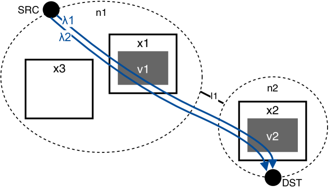
(a) First placement

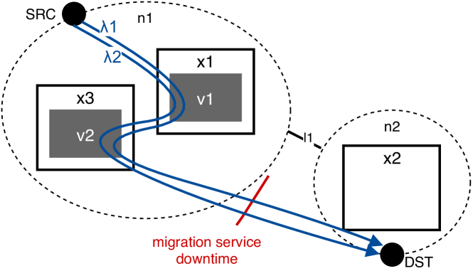
(b) Migration during second placement

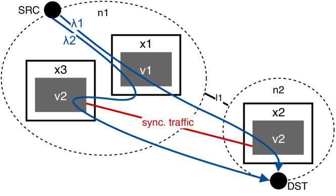
(c) Replication during second placement

Figure 1: Examples of different possible scenarios for the model

3.2 Migrations and replications

To better understand the model, let us now illustrate an example (shown in Fig. 1a) of an SFC is providing service to traffic demands $\lambda 1$ and $\lambda 2$ with two chained VNFs, $v1$ and $v2$ instantiated in server $x1$, from node $n1$, and server $x2$ from node $n2$, respectively. Depending on the functionality, every VNF can be of a different type $t$, however for simplification in this example, we assume all VNFs are of the same type $t$, so they all require the same amount resources. The service delay is calculated as the sum of propagation delays, processing delays and service interruption delays. As an example, assuming $D_{l}$ is the propagation delay of a link $l$ and $d_{x,v}^{\text{pro}}(\lambda)$ is the processing delay experienced by a traffic demand $\lambda$ traversing a VNF $v$ on a server $x$, then, the delay for traffic demand $\lambda_{1}$ using that specific path $p$ is $\hat{d}_{p}^{\lambda_{1}}=D_{l1}+d_{x1,v1}^{\text{pro}}(\lambda 1)+d_{x2,v2}^{\text{pro}}(\lambda 1)$. In this phase, which is taken as the initial placement for the second phase, we do not consider delays caused by service interruptions, since there are no migrations yet.

For the second phase, the traffic demands change, so the current VNFs in the network have the possibility to be either be migrated or replicated. An example is shown in Fig. 1b, where VNF $v2$ is migrated from server $x2$ to server $x3$. From the delay point of view, here because a service interruption ocurred due to active flows are stopped, a delay will be added and the new resulting service delay. Another example is shown in Fig. 1c, where instead of migrating, the VNF $v2$ is replicated into server $x3$ and only traffic demand $\lambda 2$ is routed to the new replica location. In this case, there is synchronization traffic added between both VNFs $v2$ to maintain their states synchronized.

3.3 Traffic demand model and time series forecasting

We assume that every source destination pair of nodes within the ISP network generates a certain number of traffic demands with specific bandwidth. The traffic demands data samples are generated using a lognormal distribution with a time-varying mean and variance, which simulates the behavior of common traffic patterns in the internet . The time-varying mean values are obtained using superposition of sinusoidal functions, i.e.:

$$y(t)=\alpha+\sum_{k=1}^{n}\beta_{k}\cdot\sin(\omega_{k}^{t}+\phi_{k})$$ (1)

, where $\alpha$ is a constant amplitude, $\beta_{k}$ and $\phi_{k}$ are frequency dependent constants, and $n$ the number of frequency components, in our case equal to 2. We generate 24 data samples per period simulating one day. An example of a resulting function is shown in Fig. 2.

In the first scenario, during the first placement the VNFs are allocated based on the observed traffic at that specific time step. In the second scenario, the VNFs are allocated assuming the demands values are at the 80% of the specific maximum traffic demand value instead of considering the real observed values. This let us consider this case as the most conservative one, since an overprovisioning of resources will occur in most of the cases. In the third scenario, the VNFs are allocated considering the predicted traffic demand values after $\Delta t$ instead of the observed ones. Then, the resulting placement from the three scenarios during this first placement is used as initial condition for the optimization of the second phase, where in all cases only the the real observed values are considered.

For the last scenario, a time series forecasting problem is modelled where a certain number of periods $D-1$ are used for training and one period for evaluation. We specifically use one LSTM network for every traffic demand with input and output sizes of 1 unit and 8 units in a hidden layer. The model uses Rectified Linear Unit (ReLU) as the activation function and is fit with Adam optimizer and optimized using the mean squared error (mse) loss function. The batch size for the model is 4 and the validation data is 10% of the total. The number of epochs is not constrained, instead an early stopping function is used with a minimum delta of 0.001 and a patience of 10 epochs. Specific parameters are later described during the evaluation of the model.

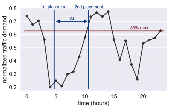
Figure 2: Normalized traffic demand example

Table 1: Parameters and variables notation

Param.	Meaning
$\mathbb{N}$	set of nodes: $\mathbb{N}=\{1,...,N\}$, $n\in\mathbb{N}$.
$\mathbb{X}$	set of servers: $\mathbb{X}=\{1,...,X\}$, $x\in\mathbb{X}$.
$\mathbb{L}$	set of links: $\mathbb{L}=\{1,...,L\}$, $\ell\in\mathbb{L}$.
$\mathbb{P}$	set of admissible paths: $\mathbb{P}=\{1,...,P\}$, $p\in\mathbb{P}$.
$\mathbb{S}$	set of SFCs: $\mathbb{S}=\{1,...,S\}$, $s\in\mathbb{S}$.
$\mathbb{T}$	set of VNF types: $\mathbb{T}=\{1,...,T\}$, $t\in\mathbb{T}$.
$\mathbb{V}_{s}$	ordered set, $v\in\mathbb{V}_{s}$ is the $v$th VNF in set $\mathbb{V}_{s}$.
$\Lambda$	set of traffic demands: $\Lambda=\{1,...,\Lambda\}$, $\lambda\in\Lambda$.
$\Lambda_{s}\subseteq\Lambda$	subset of traffic demands $\lambda\in\Lambda_{s}$ for SFC $s\in\mathbb{S}$.
$\mathbb{N}_{p}\subseteq\mathbb{N}$	subset of ordered nodes in path $p\in\mathbb{P}$.
$\mathbb{X}_{n}\subseteq\mathbb{X}$	subset of servers attached to node $n\in\mathbb{N}$.
$\mathbb{X}_{p}\subseteq\mathbb{X}$	subset of ordered servers in path $p\in\mathbb{P}$.
$\mathbb{X}_{C}\subseteq\mathbb{X}$	subset of servers located at the cloud.
$\mathbb{P}_{s}\subseteq\mathbb{P}$	subset of admissible paths $p\in\mathbb{P}_{s}$ for $s\in\mathbb{S}$.
$T_{p}^{\ell},T_{p}^{n,m}$	binary, 1 if path $p\in\mathbb{P}$ traverses link $\ell\in\mathbb{L}$ and 1 if connects node $n\in\mathbb{N}$ and $m\in\mathbb{N}$ as source and destination path nodes respectively.
$\Gamma_{t(v)}^{\mathrm{pro}},\Gamma_{t(v)}^{\mathrm{syn}}$	continuous, load ratio of a VNF of type $t\in V_{t}$ and traffic ratio for synchronization traffic between two VNFs of type $t\in V_{t}$, respectively.
$\Theta_{t(v)}^{s}$	integer, overhead for VNF $v\in\mathbb{V}_{s}$ of type $t\in V_{t}$.
$C_{\ell}^{\mathrm{max}},C_{x}^{\mathrm{max}}$	integers, maximum capacity of link $\ell\in\mathbb{L}$ and of server $x\in\mathbb{X}$, respectively.
$C_{x,t(v)}^{\mathrm{proq,max}}$	integer, maximum processing capacity that can be assigned by a server $x$ to a VNF of type $t$
$D_{\ell}$	continuous, propagation delay of link $\ell\in\mathbb{L}$.
$D_{s}^{\mathrm{max}},D^{\mathrm{dwt}}$	continuous, max. service delay of a SFC $s\in\mathbb{S}$ and service downtime duration caused by a migration, respectively.
$D_{t(v)}^{\mathrm{pro,max}}$	continuous, maximum allowed processing delay for a VNF of type $t$.
$D_{t(v)}^{\mathrm{proq}},D_{t(v)}^{\mathrm{prox}}$	continuous, delay of a VNF $v$ of type $t$ due to queues and processing, respectively.
Vars.	Meaning
$z_{p}^{s}$	binary, 1 if SFC $s$ uses path $p\in\mathbb{P}_{s}$.
$z_{p}^{\lambda,s}$	binary, 1 if traffic demand $\lambda$ from SFC $s$ uses path $p\in\mathbb{P}_{s}$.
$f_{x}$	binary, 1 if server $x$ is used, 0 otherwise.
$f_{x}^{v,s}$	binary, 1 if VNF $v\in\mathbb{V}_{s}$ from SFC $s$ is allocated at server $x\in\mathbb{X}$, 0 otherwise.
$f_{x,\lambda}^{v,s}$	binary, 1 if VNF $v\in\mathbb{V}_{s}$ from SFC $s$ is used at server $x\in\mathbb{X}$ by traffic demand $\lambda$, 0 otherwise.
$h_{p}^{v,s}$	binary, 1 if VNF $v\in\mathbb{V}_{s}$ from SFC $s$ uses path $p\in\mathbb{P}$ for state synchronization, 0 otherwise.
$d_{p}^{\lambda,s}$	continuous, service delay of a traffic demand $\lambda$ in path $p$.
$u_{\ell}$, $u_{x}$	continuous, utilization of a link $\ell\in\mathbb{L}$ and server $x\in\mathbb{X}$, respectively.

4 Problem Formulation

We model the network as $\mathbb{G}=(\mathbb{N}\cup\mathbb{X},\mathbb{L})$ where $\mathbb{N}=\{1,...,N\}$ is a set of nodes, $\mathbb{X}=\{1,...,X\}$ is a set of servers and $\mathbb{L}=\{1,...,L\}$ is a set of directed links. Specifically, $\mathbb{X}_{n}$ is a subset of servers $x\in\mathbb{X}$ attached to node $n\in\mathbb{N}$. We denote the set of all SFCs as $\mathbb{S}=\{1,...,S\}$, where a specific SFC $s\in\mathbb{S}$ is an ordered set of VNFs $\mathbb{V}_{s}=\{1,...,V_{s}\}$, each VNF being of type $t$, $t\in\mathbb{T}$, $\mathbb{T}=\{1,...,T\}$, where $v\in\mathbb{V}_{s}$ is the $v$^th VNF in set $V_{s}$. Table 1 summarizes the notations. It should be noted that the model is written such that it can be efficiently used in optimization solvers. For instance, the big M method is avoided when possible or its value is minimized in order to avoid numerical issues with the solver.

4.1 Objective Function

We define the joint optimization problem as the minimization of the sum of the number of migrations and replications, i.e.,

$$\text{\emph{minimize}}:\quad \sum_{s\in\mathbb{S}}\sum_{v\in\mathbb{V}_{s}}\bigg{[}W_{m}\sum_{x\in\mathbb{X}}F_{x}^{v,s}(1-f_{x}^{v,s})$$ (2a)

$$+W_{r}\Big{[}\big{(}\sum_{x\in\mathbb{X}}f_{x}^{v,s}\big{)}-1\Big{]}\bigg{]}$$ (2b)

$$+W_{c}\sum_{x\in\mathbb{X}_{C}}\sum_{s\in\mathbb{S}}\sum_{v\in\mathbb{V}_{s}}f_{x}^{v,s}$$ (2c)

, where the variable $f_{x}^{v,s}$ specifies if a VNF $v$ from service chain $s$ is allocated in server $x$. Since the optimization process follows two different phases, after the first placement we take the value of variables $f_{x}^{v,s}$ and convert them into the input parameters $F_{x}^{v,s}$ for the next placement step, i.e.

$$\forall s\in\mathbb{S},\forall v\in\mathbb{V}_{s},\forall x\in\mathbb{X}:f_{x}^{v,s}\Rightarrow F_{x}^{v,s}$$ (3)

The parameter $F_{x}^{v,s}$ determines if a VNF $v$ of a service chain $s$ was placed on server $x$ during the initial placement. In this way, the first term of the equation (2) counts the number of migrations, the second term counts the number of replications and the third term counts the number of functions allocated in cloud servers (here only $\mathbb{X}_{C}$ subset is considered). We next follow up with the definition of constraints.

4.2 General Constraints

The general constraints are related to the traffic routing, the VNF placement and the mapping between VNFs and paths.

4.2.1 Routing

For a given network, the input set $p\in\mathbb{P}_{s}$ is the set of all pre-calculated paths for SFC $s$. The binary variable $z_{p}^{\lambda,s}=1$ indicates, that a traffic demand $\lambda\in\Lambda_{s}$ of the SFC $s$ is using path $p\in\mathbb{P}_{s}$. The first routing constraint specifies that each traffic demand $\lambda\in\Lambda_{s}$ from SFC $s\in\mathbb{S}$ has to use only one path $p\in\mathbb{P}_{s}$, i.e.:

$$\forall s\in\mathbb{S},\forall\lambda\in\Lambda_{s}:\sum_{p\in\mathbb{P}_{s}}z_{p}^{\lambda,s}=1$$ (4)

Then, the next constraint takes the activated paths from the variable $z_{p}^{\lambda,s}$ and activates the path for a certain SFC $s$:

$$\forall s\in\mathbb{S},\forall p\in\mathbb{P}_{s},\forall\lambda\in\Lambda_{s}:z_{p}^{\lambda,s}\leq z_{p}^{s}\leq\sum_{\lambda^{\prime}\in\Lambda_{s}}z_{p}^{\lambda^{\prime},s}$$ (5)

This forces $z_{p}^{s}$ to be 1 when at least one traffic demand is using path $p$, whereas the right side forces to $z_{p}^{s}$ to be 0 when no traffic demand $\lambda$ is using path $p$.

4.2.2 VNF placement

VNF placement is modeled using the binary variable $f_{x,\lambda}^{v,s}$, which has only value 1, if VNF $v$ from SFC $s$ is allocated at server $x\in\mathbb{X}$ and used by traffic demand $\lambda\in\Lambda_{s}$. Similar to (4), the next constraint defines that each traffic demand $\lambda\in\Lambda_{s}$ from SFC $s\in\mathbb{S}$ traverses every VNF $v\in\mathbb{V}_{s}$ in only one specific server $x\in\mathbb{X}$:

$$\forall s\in\mathbb{S},\forall v\in\mathbb{V}_{s},\forall\lambda\in\Lambda_{s}:\sum_{x\in\mathbb{X}}f_{x,\lambda}^{v,s}=1$$ (6)

Then, similarly to (5), the next constraint takes the activated VNFs for each traffic demand from the variable $f_{x,\lambda}^{v,s}$ and activates the VNF for a certain SFC $s$ as follows:

$$\begin{split}\forall s\in\mathbb{S},\forall v\in\mathbb{V}_{s},\forall x\in\mathbb{X},\forall\lambda\in\Lambda_{s}:\\ f_{x,\lambda}^{v,s}\leq f_{x}^{v,s}\leq\!\!\!\!\sum_{\lambda^{\prime}\in\Lambda_{s}}f_{x,\lambda^{\prime}}^{v,s}\end{split}$$ (7)

, where the left side forces to $f_{x}^{v,s}$ to be 1 when at least one traffic demand $\lambda\in\Lambda_{s}$ is using VNF $v\in\mathbb{V}_{s}$ at server $x\in\mathbb{X}$ and the right side forces to $f_{x}^{v,s}$ to be 0 when no traffic demand is using that specific VNF $v$ on server $x$. Likewise, we determine if a server is being used or not by constraining the variable $f_{x}$ as:

$$\forall x\in\mathbb{X}:\frac{1}{|\mathbb{S}||\mathbb{V}_{s}|}\sum_{s\in\mathbb{S}}\sum_{v\in\mathbb{V}_{s}}f_{x}^{v,s}\leq f_{x}\leq\sum_{s\in\mathbb{S}}\sum_{v\in\mathbb{V}_{s}}f_{x}^{v,s}\text{ ,}$$ (8)

where $f_{x}$ is 1 if at least one VNF from any SFC is allocated at server $x\in\mathbb{X}$, 0 otherwise.

4.2.3 Mapping VNFs to paths

The next equation maps the activated VNF to the activated paths defined in the previous constraints. The first one defines how many times a VNF can be replicated:

$$\forall s\in\mathbb{S},\forall v\in\mathbb{V}_{s}:\sum_{x\in\mathbb{X}}f_{x}^{v,s}\leq R_{t(v)}\sum_{p\in\mathbb{P}_{s}}z_{p}^{s}+1-R_{t(v)}$$ (9)

, where $R_{t(v)}$ specifies if a certain VNF $v$ of type $t$ is replicable. When $R_{t(v)}$ is 0, the total number of activated VNFs $v\in\mathbb{V}_{s}$ from SFC $s\in\mathbb{S}$ is $\sum_{x\in\mathbb{X}}f_{x}^{v,s}\leq 1$. In case the VNF is replicable, then the maximum number of replicas is limited by the total number of activated paths $\sum_{p\in\mathbb{P}_{s}}z_{p}^{s}$ for that specific SFC $s$. The next constraint activates the VNFs on the activated paths:

$$\forall s\in\mathbb{S},\forall p\in\mathbb{P}_{s},\forall\lambda\in\Lambda_{s},\forall v\in\mathbb{V}_{s}:z_{p}^{\lambda,s}\leq\sum_{x\in\mathbb{X}_{p}}f_{x,\lambda}^{v,s}$$ (10)

If the variable $z_{p}^{\lambda,s}$ is activated, then every VNF $v\in\mathbb{V}_{s}$ from SFC $s\in\mathbb{S}$ has to be activated in some server $x\in\mathbb{X}_{p}$ from the path $p\in\mathbb{P}$ for a specific traffic demand $\lambda$. When $z_{p}^{\lambda,s}$ is deactivated, then no VNFs can be placed for that specific traffic demand. The last general constraint controls that all VNFs $V_{s}$ from a specific SFC $s$ are traversed by every traffic demand $\lambda\in\Lambda_{s}$ in the given order, i.e.:

$$\begin{split}\forall s\in\mathbb{S},\forall\lambda\in\Lambda_{s},\forall p\in\mathbb{P}_{s},\forall v\in\mathbb{V}_{s},\forall n,m\in\mathbb{N}:\\ \Bigg{(}\sum_{m=1}^{n}\sum_{y\in\mathbb{X}_{m}}\!f_{y,\lambda}^{(v-1),s}\!\!\Bigg{)}-\!\!\!\sum_{x\in\mathbb{X}_{n}}\!\!f_{x,\lambda}^{v,s}\geq z_{p}^{\lambda,s}\!-1\left\{\begin{array}[]{ll}1<v\leq|\mathbb{V}_{s}|\\ n\neq m\end{array}\right.\end{split}$$ (11)

, where the variable $z_{p}^{\lambda,s}$ activates the ordering constraint side (left side) when is 1 and deactivates it, otherwise. Then, if path $p\in\mathbb{P}$ is activated, the ordering is checked for every traffic demand $\lambda\in\Lambda_{s}$ individually by using the variable $f_{x,\lambda}^{v,s}$. Hence, for every traffic demand $\lambda$ of SFC $s$, the $v$^th VNF is allocated at server $x\in\mathbb{X}_{n}$ only if the previous $(v-1)$^th VNF is allocated at any server $y\in\mathbb{X}_{m}$, where $m$ is the i^th node from 1 until $n$ traversed by path $p$. It should be noted, that the correct sequence of VNFs relies on the correct sequence of subset of servers, i.e. $x\in\mathbb{X}_{n}$. This assumes that the correct sequence of VNFs inside these subsets is organized by the local routing, which may be located at the node $n$ or at a local switch not modeled in detail.

4.3 Traffic and Performance Constraints

4.3.1 Synchronization traffic

When performing replications of VNFs, the stateful states between the original and replicas has to be maintained in order to be reliable against VNF failures and avoiding the loss of information. For this reason, we consider that when a VNF is replicated, the generated synchronization traffic between replicas and the original has to be also considered. The amount of the state synchronization traffic depends on the state space and its time dynamic, where it is assumed, that each VNF has full knowledge on the state of all its instances used to implement the VNF $v\in\mathbb{V}_{s}$. Let us assume, that this amount is proportional to the total traffic offered to the SFC weighted by an synchronization ratio $\Gamma_{t(v)}^{\mathrm{syn}}$, which depends on the type of VNF $t$. In summary, the directional traffic from a VNF to its replica is given by $\Gamma_{t(v)}^{\mathrm{syn}}|\Lambda_{s}|$, and its routing should be optimized within the network.

In order to know if the same VNF $v\in\mathbb{V}_{s}$ from SFC $s$ is placed in two different servers $x\in\mathbb{X}$ and $y\in\mathbb{X}$, we define:

$$\begin{split}\forall s\in\mathbb{S},\forall v\in\mathbb{V}_{s},\forall x\in\mathbb{X},\forall y\in\mathbb{X}:\\ g_{x,y}^{v,s}=f_{x}^{v,s}f_{y}^{v,s}\text{, \quad for }y\!\neq\!x\end{split}$$ (12)

, where the variable $g_{x,y}^{v,s}$ is 1 only when both variables $f_{x}^{v,s}$ and $f_{y}^{v,s}$ are also 1, and 0 otherwise. In this way, this variable is used to know if two different servers have the same VNF placed, which means that model is allocating one replica. We use the well-known linearization method when multiplying two binary variables. In case $g_{x,y}^{v,s}=1$, we need to carry the synchronization traffic from server $x$ to $y$, by selecting only one predefined path between them, i.e.:

$$\begin{split}\forall s\in\mathbb{S},\forall v\in\mathbb{V}_{s},\forall n,m\in\mathbb{N},\forall x\in\mathbb{X}_{n},\forall y\in\mathbb{X}_{m}:\\ g_{x,y}^{v,s}\leq\sum_{p\in\mathbb{P}}h_{p}^{v,s}\cdot T_{p}^{n,m}\leq 1\text{,\quad for }n\neq m\end{split}$$ (13)

$$\begin{split}\forall s\in\mathbb{S},\forall v\in\mathbb{V}_{s},\forall n,m\in\mathbb{N}:\\ \sum_{p\in\mathbb{P}}h_{p}^{v,s}\cdot T_{p}^{n,m}\leq\sum_{x\in\mathbb{X}_{n}}\sum_{y\in\mathbb{X}_{m}}g_{x,y}^{v,s}\text{,\quad for }n\neq m\end{split}$$ (14)

, where the constant $T_{p}^{n,m}=1$ indicates, that the path $p\in\mathbb{P}$ exists which connects servers $x\in\mathbb{X}_{n}$ and $y\in X_{m}$ using the shortest path between nodes $n$ and $m$. The right term of (13) guarantees that only one path $p\in\mathbb{P}$ is selected by variable $h_{p}^{v,s}$. Moreover, (14) guarantees that this path is only used if at least one $g_{x,y}^{v,s}$ is 1. Note that $h_{p}^{v,s}$ is a binary variable used for every VNF $v$ of SFC $s$.

4.3.2 Link and server utilization

The utilization of a link is calculated as follows:

$$\begin{split}\forall\ell\in\mathbb{L}:u_{\ell}=\frac{1}{C_{\ell}^{\mathrm{max}}}\sum_{s\in\mathbb{S}}\sum_{p\in\mathbb{P}_{s}}\sum_{\lambda\in\Lambda_{s}}\lambda\cdot T_{p}^{\ell}\cdot z_{p}^{\lambda,s}+\\ \frac{1}{C_{\ell}^{\mathrm{max}}}\sum_{p\in\mathbb{P}}T_{p}^{\ell}\sum_{s\in\mathbb{S}}\sum_{v\in\mathbb{V}_{s}}\Gamma_{t(v)}^{\mathrm{syn}}\cdot|\Lambda_{s}|\cdot h_{p}^{v,s}\leq 1\text{ ,}\end{split}$$ (15)

where $\lambda\cdot T_{p}^{\ell}$ adds the traffic demands from SFC $s\in\mathbb{S}$ when a path $p\in\mathbb{P}_{s}$ traverses the link $\ell\in\mathbb{L}$. Then, the variable $z_{p}^{\lambda,s}$ specifies if the traffic demand $\lambda$ from SFC $s$ is using path $p$. The second term is the sum of the extra traffic generated due to the state synchronization between VNFs $v\in\mathbb{V}_{s}$ from SFC $s$, which is proportional to its total traffic $|\Lambda_{s}|$ multiplied by the synchronization traffic ratio $\Gamma_{t(v)}^{\mathrm{syn}}$ of the VNF of type $t$. This traffic is only added, if the variable $h_{p}^{v,s}$ is 1, which indicates that path $p\in\mathbb{P}$ is used for synchronization by a VNF $v$ from SFC $s$, and the link $\ell\in\mathbb{L}$ belongs to this path. Both summation terms are divided by the maximum link capacity $C_{\ell}^{\mathrm{max}}$ to restrict the utilization.

The processing load of a server is derived as

$$\gamma_{x}=\sum_{s\in\mathbb{S}}\sum_{v\in\mathbb{V}_{s}}\Big{(}\Gamma_{t(v)}^{\mathrm{pro}}\sum_{\lambda\in\Lambda_{s}}\lambda\cdot f_{x,\lambda}^{v,s}+\Theta_{t(v)}^{s}\cdot f_{x}^{v,s}\Big{)}$$ (16)

, where the first term sums the traffic $\lambda\in\Lambda_{s}$ that is using the VNF $v\in\mathbb{V}_{s}$ from SFC $s\in\mathbb{S}$ at server $x\in\mathbb{X}$, which is determined by the variable $f_{x,\lambda}^{v,s}$, and multiplied by the processing load ratio $\Gamma_{t(v)}^{\mathrm{pro}}$ of the VNF of type $t$. The second term adds the overhead generated by the VM where the VNF is running and is only added, when the variable $f_{x}^{v,s}$ determines that this VNF is placed in server $x$. Then, the utilization follows to be given by

$$\forall x\in\mathbb{X}:u_{x}=\frac{\gamma_{x}}{C_{x}^{\mathrm{max}}}\leq 1\text{ ,}$$ (17)

where $C_{x}^{\mathrm{max}}$ is the maximum processing capacity.

4.3.3 Service delay

Since every service has a maximum allowed delay $D_{s}^{\mathrm{max}}$ specified in the SLA agreement, in case of exceeding it, some penalty costs are applied. In our model, and for simplicity, we take into account the propagation delay due to the traversed links, the processing delay that every VNF requires in the servers and, where applicable, the downtime delays caused by the interruption of the service during the migrations of VNFs.

Processing delay: The processing delay $d_{x,v,s}^{\mathrm{pro}}$ of a VNF $v$ in a server $x$ depends, on the one side, on the amount of traffic being processed by a specific VNF, described by $d_{x,v,s}^{\mathrm{proq}}$, and on $d_{x,v,s}^{\mathrm{prox}}$, which is related to the VNF type and the total server load $u_{x}$, given as

$$\forall s\in\mathbb{S},\forall v\in\mathbb{V}_{s},\forall x\in\mathbb{X}_{p}:d_{x,v,s}^{\mathrm{pro}}=d_{x,v,s}^{\mathrm{proq}}+d_{x,v,s}^{\mathrm{prox}}$$ (18a)

$$d_{x,v,s}^{\mathrm{proq}}=D_{t(v)}^{\mathrm{proq}}\frac{\Gamma_{t(v)}^{\mathrm{pro}}\cdot\sum_{\lambda\in\Lambda_{s}}f_{x,\lambda}^{v,s}\cdot\lambda}{C_{x,t(v)}^{\mathrm{proq,max}}}$$ (18b)

$$d_{x,v,s}^{\mathrm{prox}}=D_{t(v)}^{\mathrm{pro\_x,min}}\cdot f_{x}^{v,s}+D_{t(v)}^{\mathrm{prox}}\cdot u_{x}$$ (18c)

In (18b), the numerator of $d_{x,v,s}^{\mathrm{proq}}$ determines the total processing load assigned to the VNF of type $t$, which is controlled by the variables $f_{x,\lambda}^{v,s}$. Thus, if the assigned processing load is equal to $C_{x,t(v)}^{\mathrm{proq,max}}$, the VNF adds the processing delay $D_{t(v)}^{\mathrm{proq}}$. The second delay term, given in (18c), adds the load independent minimum delay associated to the usage of a type of this VNF, and a delay part which increases with the server utilization. As a consequence the processing delay $d_{x,v,s}^{\mathrm{pro}}(\vec{\lambda})$ depends on the server $x$, the used VNF type and linearly increases with increasing traffic. Furthermore, the dependency on all traffic demands is denoted by the vector $\vec{\lambda}$, which is omitted for simplicity in (18).

Downtime duration: If a VNF $v$ of SFC $s$ has to be migrated, we assume an interruption of the service with duration $D^{\mathrm{dwt}}$. Thus, the total service downtime will consider the migration of all VNFs in that SFC which yields a constraint as follows:

$$\forall s\in\mathbb{S}:d_{s}^{\mathrm{dwt}}=D^{\mathrm{dwt}}\sum_{x\in\mathbb{X}}\sum_{v\in\mathbb{V}_{s}}F_{x}^{v,s}(1-f_{x}^{v,s})$$ (19)

, where the parameter $F_{x}^{v,s}$ determines if a VNF $v$ was placed on server $x$ during the first placement. Thus, if a VNF migrates to another server $y\neq x$, the variable $f_{x}^{v,s}$ is equal to zero and the service downtime $D^{\mathrm{dwt}}$ has to be taken into account.

Total delay: Because the model allows that different traffic demands per service can be assigned to different paths, we define individual end-to-end delay $\hat{d}_{p}^{\lambda,s}$ for every traffic demand, as follows:

$$\begin{split}\forall s\in\mathbb{S},\forall\lambda\in\Lambda_{s},\forall p\in\mathbb{P}_{s}:\\ \hat{d}_{p}^{\lambda,s}=\sum_{\ell\in\mathbb{L}}D_{\ell}\cdot T_{p}^{\ell}+\sum_{x\in\mathbb{X}_{p}}\sum_{v\in\mathbb{V}_{s}}d_{x,v,s}^{\mathrm{pro}}(\vec{\lambda})\cdot f_{x,\lambda}^{v,s}+d_{s}^{\mathrm{dwt}}\end{split}$$ (20)

The first term is the propagation delay, where $D_{\ell}$ is the delay of the link $\ell$, and $T_{p}^{\ell}$ specifies if the link $\ell$ is traversed by path $p\in\mathbb{P}_{s}$. The second term adds the processing delays caused by all VNFs from the SFC placed on the servers $x\in\mathbb{X}_{p}$, in which the variable $f_{x,\lambda}^{v,s}$ has to ensure that the demand $\lambda$ is processed at a specific server $x$. Finally, the third term is the total downtime duration due to the migrations of that service chain. It should be noted that the second term of (20) includes a nonlinear relation between the binary variable $f^{v,s}_{x,\lambda}$ and the delay variable $d_{x,v,s}^{\mathrm{pro}}$, which also depends on all decision variables $f^{v{{}^{\prime}},s{{}^{\prime}}}_{x,\lambda{{}^{\prime}}}$. To solve that, we introduce a new delay variable $d_{x,\lambda}^{v,s}$, which is bounded as follows:

$$d_{x,v,s}^{\mathrm{pro}}-D_{t(v)}^{\mathrm{pro,max}}(1-f_{x,\lambda}^{v,s})\leq d_{x,\lambda}^{v,s}\leq D_{t(v)}^{\mathrm{pro,max}}\cdot f_{x,\lambda}^{v,s}$$ (21)

If the VNF is selected at server $x$ by $f_{x,\lambda}^{v,s}=1$, the variable is lower bounded by the exact delay $d_{x,v,s}^{\mathrm{pro}}$ and upper bounded by the maximum VNF delay $D_{t(v)}^{\mathrm{pro,max}}$. Since $d_{x,v,s}^{\mathrm{pro}}\leq d_{x,\lambda}^{v,s}\leq D_{t(v)}^{\mathrm{pro,max}}$, the specific delay of a VNF can be restricted. If the VNF is not selected, i.e., $f_{x,\lambda}^{v,s}=0$, the variable has value $d_{x,\lambda}^{v,s}=0$, since the constant $D_{t(v)}^{\mathrm{pro,max}}$ makes the left size of (21) to be negative. Hence, the end-to-end delay is mapped to an upper and lower bounded variable $d_{p}^{\lambda,s}$ given as

$$\begin{split}\forall s\in\mathbb{S},\forall\lambda\in\Lambda_{s},\forall p\in\mathbb{P}_{s}:\\ d_{p}^{\lambda,s}=\sum_{\ell\in\mathbb{L}}D_{\ell}\cdot T_{p}^{\ell}+\sum_{x\in\mathbb{X}_{p}}\sum_{v\in\mathbb{V}_{s}}d_{x,\lambda}^{v,s}+d_{s}^{\mathrm{dwt}}\quad\text{,}\end{split}$$ (22)

in which the bounding feature is used in the optimization scenarios described next.

5 Online Heuristic Approaches

Since the model presented is a MILP optimization problem and these models are known to be NP-hard [4], in this section we propose a greedy algorithm to work as an online solution and, First-Fit and Random-Fit algorithms for comparison purposes.

5.1 First-Fit and Random-Fit algorithms

Both First-Fit (FF) and Random-Fit (RF) algorithms are described in Algorithm 1. While both approaches share most of the code, the FF_RF parameter specifies whether the code has to run FF or RF. The process starts with a loop where every demand from every SFC is going to be considered (line 1). The first step is to then retrieve all the paths with enough link resources to assign traffic demand $\lambda$ and that also connect both source and destination nodes (line 2). These paths are saved into $\mathbb{P}_{s}^{\prime}$, from where one admissible path $p$, first one for FF or a random one for RF, is selected (line 3). In this point, we make sure here that in this path, there are enough server resources to allocate all the VNFs for SFC $s$. Then, from that path, for every VNF $v$ from SFC $s$ (line 4) we start with the process of selecting servers for allocations. First, we retrieve all servers with enough free capacity to allocate the VNF $v$ and to provide service to demand $\lambda$ (line 5), and then we choose the first available server in FF or a random one in RF (line 6). It is to be noted here, that to satisfy VNF ordering (see equation 11), the procedure chooseServer will return a valid server from before/after the previous/next VNF allocated. While for the FF case, we assure in line 3 that there will always be a server where to allocate the next VNF in the chain, in RF case we make sure here (line 6) that after the random server selected there is still place to allocate all the rest of the VNFs from the chain in next servers in the path, or we select another server instead. In line 7, we assign the demand and the VNF to the server (i.e. equations (6) and (7)). After all the VNFs have been placed, the next step is to route traffic demand $\lambda$ to path $p$ (line 9), to finally add the synchronization traffic for the service chain (line 10).

Algorithm 1 First-Fit/Random-Fit: main(FF_RF)

1:for $s\in\mathbb{S}$, $\lambda\in\Lambda_{s}$ do

2:   $\mathbb{P}_{s}^{\prime}\leftarrow$ getAdmissiblePaths($s$, $\lambda$)

3:   $p\leftarrow$ choosePath(FF_RF, $\mathbb{P}_{s}^{\prime}$)

4:   for $v\in\mathbb{V}_{s}$ do

5:     $\mathbb{X}_{p}^{\prime}\leftarrow$ getAvailableServers($s$, $\lambda$, $v$, $p$)

6:     $x\leftarrow$ chooseServer(FF_RF, $\mathbb{X}_{p}^{\prime}$)

7:     addVNFToServer($s$, $v$, $\lambda$, $x$)

8:   end for

9:   routeDemandToPath($s$, $p$, $\lambda$)

10:   addSynchronizationTraffic($s$)

11:end for

5.2 Greedy algorithm

The greedy algorithm main function is described in Algorithm 2. The procedure starts with the natural ordering of SFCs by the total traffic demand value (line 1). This is done in order to first allocate services with lower impact on the utilization resources in order to avoid the creation of bottlenecks in servers and links during the firsts phases of the allocation. Then, it starts iterating over each service (line 2) and over each traffic demand for certain service (line 3). Then, for each traffic demand we first retrieve all paths with enough free link resources in $\mathbb{P}_{s}^{\prime}$ (line 4). Then, we choose a path $p$ inside of a loop from all retrieved paths (line 6, details explained later).This is done to ensure that in case a path cannot be used for allocating all VNFs, the algorithm tries with the next one. Once the path is selected, we start with the placement of all VNFs on the selected path. First, all the available servers for a specific VNF $v$ on path $p$ are retrieved in variable $\mathbb{X}_{p}^{\prime}$ (line 8), then we choose one server $x$ for that specific VNF in line 9 (this procedure explained later) and place the VNF (line 10). In case the VNF has been already placed by another demand of the same service, the demand is associated to that VNF, instead. Finally after all VNFs are placed, we map the demand over path (line 12). Finally, as in the previous case, the synchronization traffic for that service is added (line 15)

Algorithm 2 Greedy: main()

1:$\mathbb{S}^{\prime}$ = orderServicesByTotalDemandValue($\mathbb{S}$)

2:for $s\in\mathbb{S}^{\prime}$ do

3:   for $\lambda\in\Lambda_{s}$ do

4:     $\mathbb{P}_{s}^{\prime}\leftarrow$ getAdmissiblePaths($s$, $\lambda$)

5:     for $p\in\mathbb{P}_{s}^{\prime}$ do

6:        $p\leftarrow$ choosePath($s$, $\lambda$, $\mathbb{P}_{s}^{\prime}$) $\triangleright$ go to Alg. 3

7:        for $v\in\mathbb{V}_{s}$ do

8:          $\mathbb{X}_{p}^{\prime}\leftarrow$ getAvailableServers($s$, $\lambda$, $p$, $v$)

9:          $x\leftarrow$ chooseServer($s$, $\lambda$, $p$, $v$, $\mathbb{X}_{p}^{\prime}$) $\triangleright$ go to Alg. 4

10:          mapVNFToServer($v$ , $x$)

11:        end for

12:        mapDemandToPath($s$, $p$, $\lambda$)

13:     end for

14:   end for

15:   addSynchronizationTraffic($s$)

16:end for

Algorithm 3 Greedy: choosePath($s$, $\lambda$, $\mathbb{P}_{s}^{\prime}$)

1:$p\leftarrow$ getUsedPathDemandInitPlacement($s$, $\lambda$, $\mathbb{P}_{s}^{\prime}$)

2:if $p$ then return $p$

3:end if

4:$p\leftarrow$ getUsedPathInitialPlacement($s$, $\mathbb{P}_{s}^{\prime}$)

5:if $p$ then return $p$

6:end if

7:$p\leftarrow$ getUsedPathForSFC($s$, $\mathbb{P}_{s}^{\prime}$)

8:if $p$ then return $p$

9:end if

10:return getPathWithShortestDelay($s$, $\lambda$, $\mathbb{P}_{s}^{\prime}$)

Algorithm 4 Greedy: chooseServer($s$, $\lambda$, $p$, $v$, $\mathbb{X}_{p}^{\prime}$, A)

1:$\mathbb{X}_{p}^{\prime}\leftarrow$ removeServersPreviousVNFs($\mathbb{X}_{p}^{\prime}$)

2:$\mathbb{X}_{p}^{\prime}\leftarrow$ removeServersNextVNFs($\mathbb{X}_{p}^{\prime}$)

3:$c\leftarrow$ getCloudServer($\mathbb{X}_{p}^{\prime}$)

4:$x\leftarrow$ getUsedServerDemandInitialPlace($s$, $v$, $\lambda$, $\mathbb{X}_{p}^{\prime}$)

5:checkPosition(x, c, A) $\triangleright$ go to line 13

6:$x\leftarrow$ getUsedServerInitialPlacement($s$, $v$, $\mathbb{X}_{p}^{\prime}$)

7:checkPosition(x, c, A) $\triangleright$ go to line 13

8:$x\leftarrow$ getUsedServerForSFC($s$, $v$, $\mathbb{X}_{p}^{\prime}$)

9:checkPosition(x, c, A) $\triangleright$ go to line 13

10:if !A then return null

11:else return $\mathbb{X}_{p}^{\prime}$[0]

12:end if

13:procedure checkPosition($x$, $c$, A)

14:   if $x$ != null then

15:     if $A$ & $c$ & indexOf($x$) < indexOf($c$) then

16:        return x

17:     else if $A$ & $c$ & indexOf($x$) > indexOf($c$) then

18:        return c

19:     else return $x$

20:     end if

21:   end if

22:end procedure

When selecting a path for a specific traffic demand in line 6, the procedure described in Algorithm 3 is executed. This procedure execute the following methods in this specific order: return an already used path for the same demand $\lambda$ during the initial placement (line 1), return any used path for SFC $s$ during the initial placement (line 4), return any used path for SFC $s$ (line 7) or return the path with shortest path delay (line 10). If one method does not return a path, then the next one is executed.

Going back to Algorithm 2, when choosing a server for a specific VNF in line 9, the procedure described in Algorithm 4 is executed. In this point, we first remove servers from the set $\mathbb{X}_{p}^{\prime}$ that have already allocated VNFs before/after the current VNF in the path (lines 1 and 2), in order to satisfy with sequence order equation (11). Then, we follow up with the selection of a server from the remaining ones. Here, in case it exists, we first retrieve the cloud server $c$ in the path (line 3). Then, we retrieve a server already used for VNF $v$ and demand $\lambda$ during the initial placement (line 4) into server $x$. In line 5, we check the position in the path of that server, where the procedure is specified in line 13. This procedure receives the server $x$, the cloud server $c$ in case it exists and the boolean variable $A$ which specifies whether this is the last attempt in terms of remaining available paths. The objective here is to first check if $x$ is valid (line 14), otherwise it finishes. In case is valid, then we return $x$ if it is the last attempt $A$, if it exists a cloud server in the path and if the index of $x$ is lower than the index of $c$ in the array. In case this condition does not apply, we continue with the next condition in line 17 with the difference of checking whether $x$ is after the cloud server in the array. In that case, the cloud server is returned. If none of the previous applies, then $x$ is returned in line 19. This procedure is basically performed to make sure that in all cases there will be a location where to place VNFs which is in the cloud server, but choosing it as the last option. Continuing with line 6, similarly here we try to retrieve a server used during the initial placement for service $s$ regardless for which traffic demand and perform the same procedure like in the previous case (line 7). While the first method tries to reuse the same exact server like in the initial placement in order to avoid a migration, here we try to use a server already used by some other demand during the initial placement for the same service in order to avoid a replication. Similarly, the next case in line 8 retrieves an already used server by the same service regarless it is from initial placement or allocated during the current placement. Here again we are trying to avoid an unnecessary replication and we check again like before the position of the returned server in line 9. If none of the previous methods returned a valid server, then we return null in line 10 in order to later try with the next available path in case this is not the latest path. If it is the latest path, then we just return the first available server in the set (line 11).

5.2.1 Computational complexity

In terms of complexity from bottom to top, for the Algorithm 4 considering $V_{L}$ as the length of the longest SFC, it is in the order of $\Theta=O(V_{L}\cdot|\mathbb{X}|)$. The Algorithm 3 is in the order of $\Theta^{\prime}=O(P_{S})$ where $P_{S}$ is the number of paths per SFC. The Algorithm 2 is calculated based on the complexity of Algorithm 3 and 4, and the complexity of the synchronization traffic (line 15) which is in the order of $\Theta^{\prime\prime}=O(V_{L}\cdot|\mathbb{X}^{2}|\cdot|\mathbb{P}|)$. Considering $L_{P}$ as the length of the longest path, then the complexity of the entire Algorithm 2 is in the order of $O(|\mathbb{S}^{2}|+|\Lambda|\cdot L_{P}\cdot P_{S}\cdot[\Theta^{\prime}+V_{L}\cdot\Theta]\cdot\Theta^{\prime\prime})$, which can be simplified as $O(|\mathbb{S}^{2}|+|\Lambda|\cdot L_{P}\cdot V_{L}\cdot|\mathbb{X}^{2}|\cdot|\mathbb{P}|\cdot[P_{S}^{2}+V_{L}^{2}\cdot|\mathbb{X}|\cdot P_{S}])$.

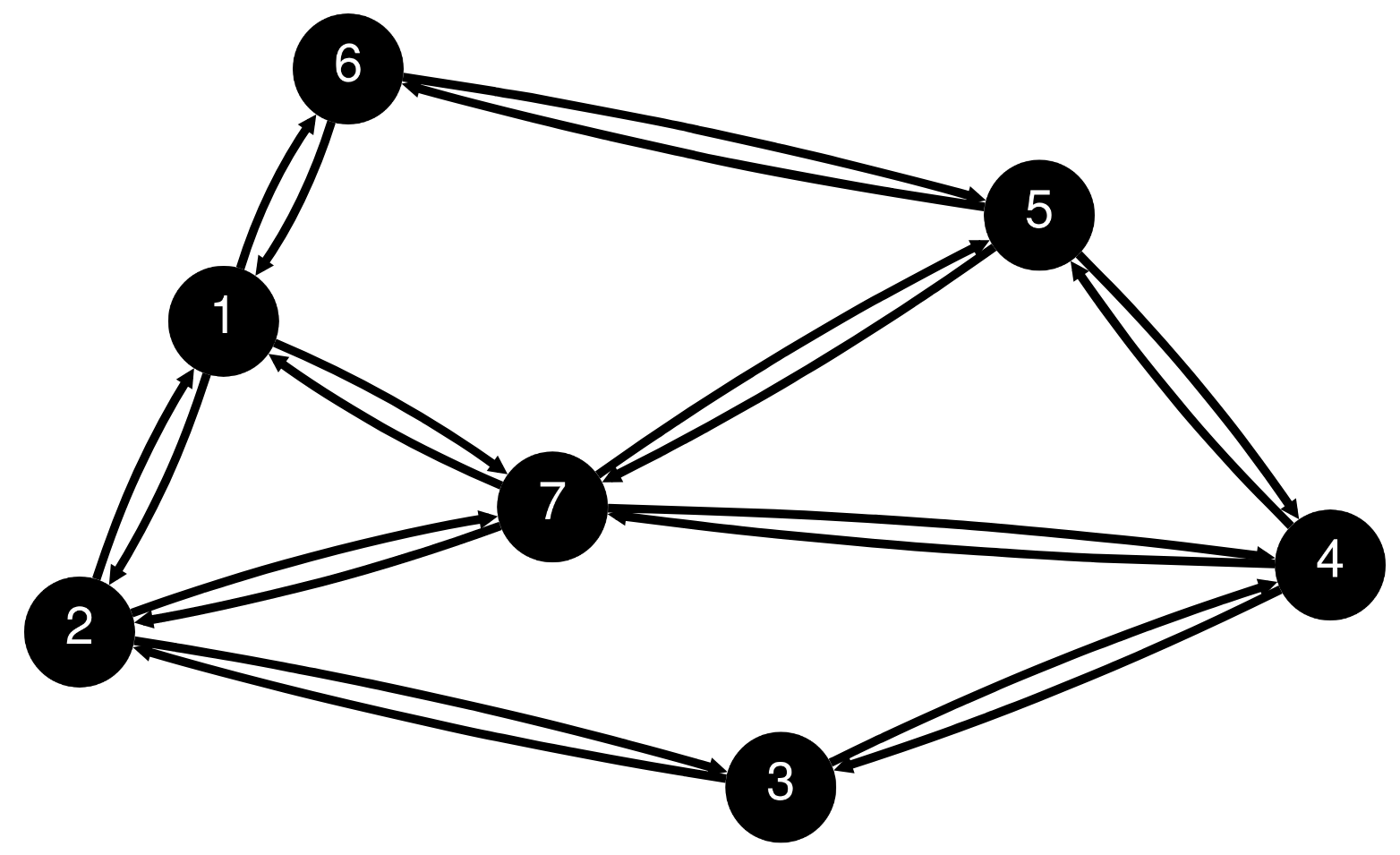
(a) N7 network

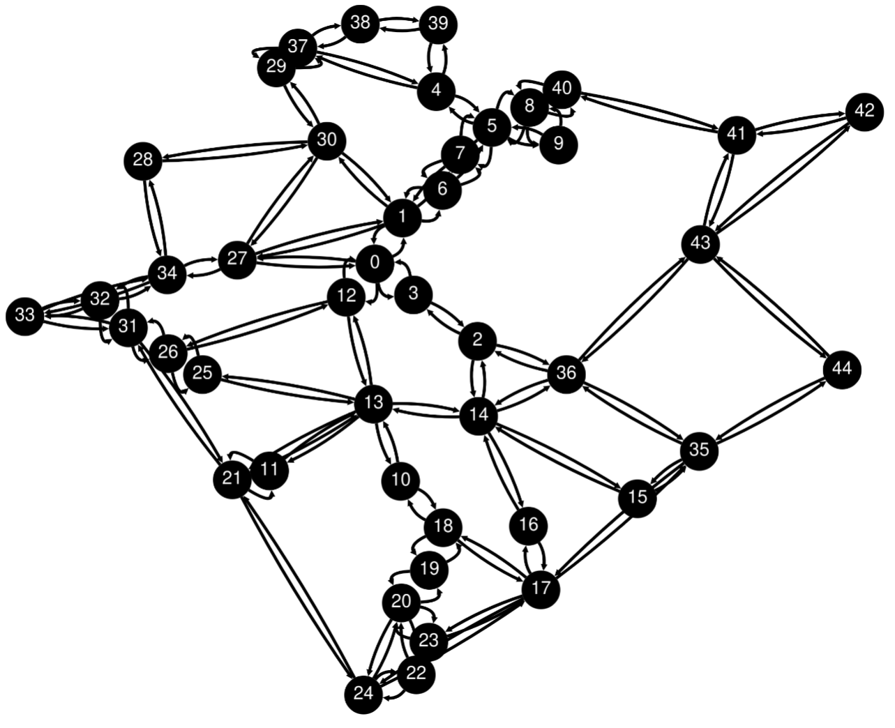
(b) N45 network

Figure 3: Network topologies used in the performance evaluation.

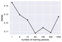
(a) RMSE

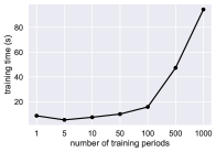
(b) Training time

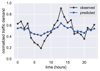
(c) Validation for 1 period

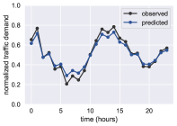
(d) Validation for 50 periods

Figure 4: Traffic prediction model results

6 Performance evaluation

We use MILP model implemented with Gurobi Optimizer tool to evaluate a smaller size network N7 (7 nodes, 20 directed links with 500 units of capacity each, see Fig. 3a) and heuristics for a larger-size network N45 (45 nodes, 140, directed links with 1000 units of capacity, Fig. 3b). In N7, every node is equipped with one server, whereas in N45 there are 8 servers per node. In both networks, we assume that all nodes can establish on-demand connectivity to a third-party cloud server of which the geographic location is determined based on the closest common locations used by cloud providers. Thus, for the 7-nodes network, in N7 the geographic locations are based regionally, such as the area of Braunschweig (Germany) for the network and the area of Frankfurt, for the cloud server, respectively. For N45, we use a modified version of Palmetto network in South Carolina, USA and the cloud server in North Virginia, USA. The propagation delay is correspondingly calculated considering the distance between nodes from their latitude and longitude using the Haversine method using 2/3 of the speed of light. We thereby assume the links used to connect to the third-party cloud have sufficient capacity for any demand, and therefore do not impact the analysis of server utilization.

For each source-destination pair of nodes, 3 paths are pre-computed that do not traverse the cloud node and 1 additional path that does. Also 2 additional paths per node are computed for the synchronization traffic between possible VNFs allocated in the cloud and in the network. The path computation is carried out in this way to make sure the model has enough freedom to allocate all SFCs in the network and at least there is one admissible path per SFC to allocate VNFs in the cloud. We assume that every source-destination pair of nodes (except the cloud node) instantiates independent SFCs with variable length from 1 to 10 VNFs depending depending on the scenario. The processing load of a certain VNF is calculated from the total amount of processed traffic in the VNF multiplied by a random load ratio ($\Gamma_{t(v)}^{\mathrm{pro}}$) between 1% and 100%. Additionally, an overhead ($\Theta_{t(v)}^{s}$) is calculated as a random percentage between 1% and 10% of the processing load [23]. The synchronization traffic between VNFs ($\Gamma_{t(v)}^{\mathrm{syn}}$) is calculated as 10% of the processing load of the VNF. The delay parameters per VNF, already explained is section 4.3.3, are specified using typical values as follows: $D_{t(v)}^{\mathrm{proq}}=3~{}ms$, $D_{t(v)}^{\mathrm{prox}}=5~{}ms$, $D_{t(v)}^{\mathrm{pro\_x,min}}=2~{}ms$ and $D_{t(v)}^{\mathrm{pro,max}}=10~{}ms$. In the networks studied, for all SFCs the service delay is constrained to $D_{s}^{\mathrm{max}}=400~{}ms$. The round trip time is, for both networks, always shorter than 5 ms which leads to a service downtime of duration $D^{\mathrm{dwt}}=27.5~{}ms$ when performing a migration, in the worst case scenario [28].

Two types of results are produced: (i) one setting all SFCs with a certain length while all servers have the same capacity and (ii) one setting all servers to the certain capacity while all SFCs have a random length. The reason for that is to independently see the effects that SFCs lengths and server capacities have on the network. In case i), the server capacities are set to 1000 for N7 and 2000 units for N45, and all SFC lengths are chosen in increments from 1 to 10. In case ii), the server capacities vary from 250 to 3000 units and every SFC is of random length between 1 and 10.

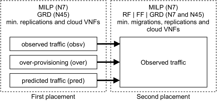
Figure 5: Optimization scenarios

6.1 Optimization scenarios

We assume that every source-destination pair of nodes generates between 1 and 3 traffic flows, with traffic demand per flow set to a random value between 1 and 100 traffic units. For each traffic demand, 24 values are generated in one time period following a lognormal distribution with time-varying mean and variance, as explained in Section 3.3. For the time series forecasting, one LSTM network is created and trained per each traffic flow for a certain number of periods, and then evaluated for 1 time period.

To determine the optimum number of required training periods, the model has been tested using from 1 to 1000 periods for training. The resulting RMSE is shown in 4a where it shows that above 50 periods of time, the performance is not improving anymore. However, the training time continues to increase with the number of training periods as expected, see Fig. 4b. Taking 1 period as the worst case and 50 as the best case, Fig. 4c and Fig. 4d show the predicted and observed normalized traffic demand values over time during the evaluation period, respectively. Here, we can see how the number of training periods impacts the accuracy of the model.

To illustrate the issues of computation time, we show the results obtained by using the CPU of a machine with an Intel Core i7-6700 and 32 GB of RAM. The total computation time considering all traffic demands for takes $\approx$7 minutes in N7, when training for 1 period and $\approx$12 minutes when training for 50 periods. For N45, it takes in total $\approx$13 hours for 50 training periods. While the specific total computational time can be improved by using GPUs or by training models in parallel, it should be noted that the network size needs to be considered when using predictions.

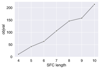
(a) Variable SFC lenght

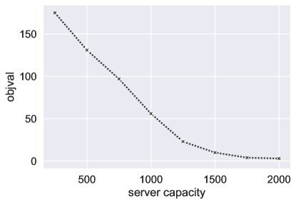
(b) Variable server capacity

Figure 6: Objective function value for obsv, over and pred scenarios in the N7 network using the MILP model.

(a) Variable SFC length

(b) Variable server capacity

Figure 7: Objective function values of RF, FF, GRD and MILP for the pred scenario in the N7 network.

From the generated traffic demand values produced for the evaluation period, three optimization scenarios are derived based on which values are considered during the first placement: i) observed values (obsv), ii) 80% of the maximum individual traffic demand values, which corresponds to overprovisioning (over) and iii) predicted values (pred). After the first placement, the second placement is carried out considering the location of the VNFs during the first placement, as explained in equation 3 and considering the new traffic demand values after a $\Delta t$ time shift from the set of traffic demand values (see Fig. 4d). In our case, the first time step for the first placement is taken randomly from the first 18 time values and $\Delta t$ is set to 6 time periods. Hence, for the first scenario obsv, only the current observed values at time $t$ are considered for the placement of VNFs. In the second scenario over, the observed values are ignored, and instead, the VNFs are placed assuming the traffic is always at the 80% of the maximum traffic demand value. The third scenario places VNFs considering the predicted traffic values after $\Delta t$.

Fig. 5) illustrates the optimization process. The second placement uses the first placement as input, and it optimizes the placement again by considering the real monitored and observed traffic demand values. The first placement is carried out using either the MILP model in N7, or the greedy algorithm (GRD) in N45. In all cases, the objective is to allocate VNF while minimizing the number of replications and the number of virtual functions placed in the cloud. In the first placement, the are no migrations from any previous step to consider. In the second placement, the MILP model in N7, and all heuristics for both networks, all by considering the same objectives which to minimizing the number of migrations, replications and cloud VNFs. Finally, for the reminder of the paper we show the results obtained from the second placement, while using the three scenarios during the first placement, as described.

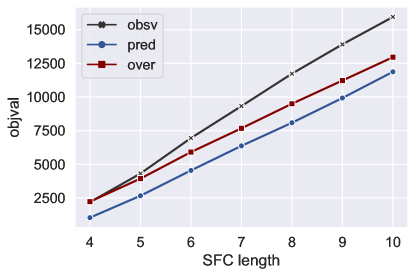
(a) Variable SFC lenght

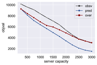
(b) Variable server capacity

Figure 8: Objective function value for obsv, over and pred scenarios in the N45 network using the GRD algorithm.

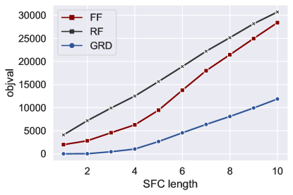
(a) Variable SFC length

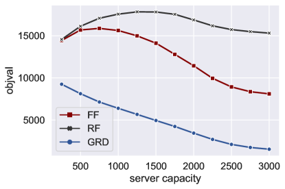
(b) Variable server capacity

Figure 9: Objective function values for RF, FF and GRD for the pred scenario in the N45 network.

6.2 Objective function

Since the objective function (equation (2)) is a joint optimization from three different weighted terms, we first show the results when minimizing all terms, so all three weights $W_{m}$, $W_{r}$ and $W_{c}$ are equal to 1. Fig. 6 shows the objective value for the three scenarios obsv, over and pred when varying the SFC lengths and when varying the server capacities in N7. It should be noted that some zero values for certain SFC lengths or server capacities are omitted in the plots due to clarity. We can observe that pred overperforms the other two cases. Between over and obsv, when the servers are overloaded the over case performs slightly better than obsv as expected, due to the overprovisioning factor.

Before analyzing the three scenarios in large network N45, let us first compare how heuristics compare to MILP model in N7. Fig. 7 shows again the objective values for pred scenario, but now comparing the MILP model with the heuristic algorithms RF, FF and GRD. Here we can see that both RF and FF are far from the optimal solution, being RF slightly better than FF in most cases.

When using the greedy algorithm for the N45 network, we compare again the three scenarios obsv, over and pred in Fig. 8. Here, we can see a more clear difference between the three cases, being again the pred scenario the one with a clear advantage compared to the other two. This case also better illustrates how over case overperforms obsv case mostly when the servers are overloaded confirming what we could slightly see with the N7 network. From Fig. 9 we can compare RF, FF and GRD, in this case for the N45 network. Different from N7, here we can see how FF outperforms RF in all cases. We see here a trend on FF working better the more free the network and servers are, but in any case the achieved values are comparable to the GRD algorithm which performs always better.

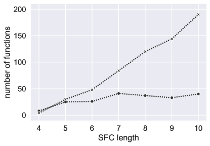
(a) Minimizing migrations

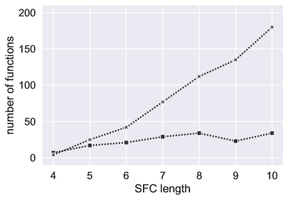
(b) Minimizing replications

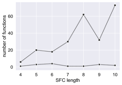
(c) Minimizing cloud VNFs

Figure 10: Number of migrations, replications and cloud VNFs for different SFC lengths in the N7 network using MILP model.

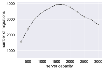
(a) Number of migrations

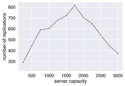
(b) Number of replications

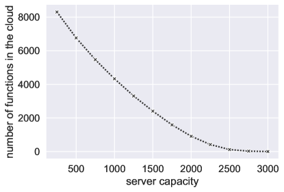
(c) Number of cloud VNFs

Figure 11: Number of migrations, replications and cloud VNFs for different server capacity in N45 network using GRD algorithm.

6.3 Migrations, Replications and Cloud VNFs

In order to better see how the model behaves individually when minimizing only one of the terms, we set a certain weight (i.e. $W_{m}$, $W_{r}$ or $W_{c}$) equal to 1, and the others close to 0 in such a way that the sum of all secondary terms is within interval $[0,1)$. By doing that, we limit the freedom of the model while, at the same time, we ensure there is no impact on the main term which value is always going to be a positive integer. In this regard, Fig. 10a shows the results in terms of number of replications (rep) and number of cloud VNFs (cld), when minimizing the number of migrations for the three scenarios obsv, over and pred and different SFC lengths in N7. By looking at over-rep and over-cld, we see how overprovisioning does not allocate replicas and places more functions in the cloud compared to other cases. In comparison, the obsv case allocates less functions in the cloud at expenses of deploying a considerable number of replicas. The pred case can be seen as a trade-off solution, as it allocates considerably less VNFs in the cloud compared to over, independently from the SFC length, and less than obsv mostly when the servers are overloaded with long SFCs. In terms of replicas, the pred requires much less resources in almost all cases compared to obsv case. When minimizing the number of replications, see Fig. 10b, the difference between pred and obsv in terms of allocations in the cloud is much smaller, but still reduces the number of migrations independently from the SFC length. Here the over case behaves quite similar to pred in number of migrations, but instead requires to allocate more cloud VNFs. When minimizing the number of functions in the cloud, see Fig. 10c, we see how pred requires much less migrations compared to the other two cases, but no remarkable difference regarding replications.

To individually see the number of migrations, replications and cloud VNFs with no influence from the weights (i.e. all terms the same weight), we now study N45 network. Fig. 11a shows how obsv case requires much more migrations compared to the other cases except when the servers are either too overloaded or too underloaded where the values become closer to over case. On the other hand, pred case requires the same number of migrations than over when the servers are overloaded and improves when there is enough free available resources. In Fig. 11b, regarding the number of replications we see that there is no much difference between pred and obsv, but over case is the one requiring significantly less replications, except for the cases where the servers are either too overloaded or too underloaded. This effect can be explained by the fact that when there are no available resources in the servers, the model cannot perform replications, and when there are more than enough available resources, the model avoids replications that are not essential. When looking at Fig. 11c, we see that there is almost no difference between obsv and pred, but the over case allocates considerably more cloud VNFs than the other two cases.

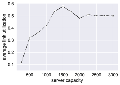
(a) Average link utilization

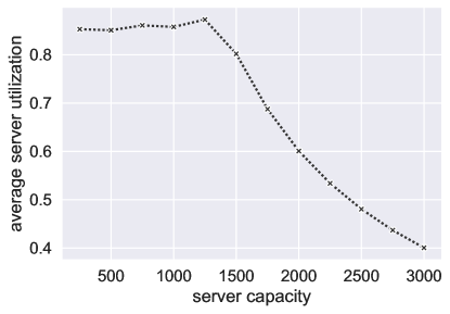
(b) Average server utilization

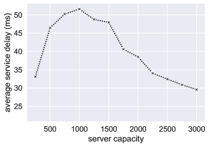
(c) Average service delay

Figure 12: Resource utilization and service delays for different server capacities in the N7 network

6.4 Resource Utilization and Service Delay

To show the difference between the three scenarios, Fig. 12a, Fig. 12b and Fig. 12c show the average link utilization, server utilization and service delay, respectively, versus a varying server capacity for N7. For both link and server utilization, the link capacity connecting to the cloud and the cloud servers are not considered. Here, in most cases when the network is not overloaded, the over case has slightly lower link utilization compared to the other cases, since this case allocates more cloud VNFs, so the edge network is less utilized and less replicas are used, so less synchronization traffic is added to the network. Between pred and obsv cases, the first one has slightly lower link utilization in some specific cases. This difference is inexistent when looking at the server utilization, and here only over case has lower utilization for the same reason as before. When comparing the three cases for the average service delay, we notice how over has the lowest delay, even though it allocates generally more cloud VNFs as we have seen before, so the propagation delay is larger. However, this case performs less migrations compared to the other cases, and therefore, there is less penalty due to service interruptions. When comparing pred with obsv, we see how pred has less service delay, so less migrations are required.

Fig. 13 shows again the same results, but this time for the N45 network. Here, we can better see the difference in the lower utilization of links of the over case compared with the other two. This is again due to the fact that overprovisioning results into a higher usage of the cloud, so the network is less utilized. This is also confirmed when looking at the average server utilization where pred and obsv cases make full usage of all server resources at the edge before using the cloud, contrary to the over case. The most interesting case is with regard the service delay, where we can see how the pred case is able to outperform over when the servers are not overloaded since the number of migrations are much lower as we could see from Fig. 11a.

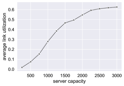
(a) Average link utilization

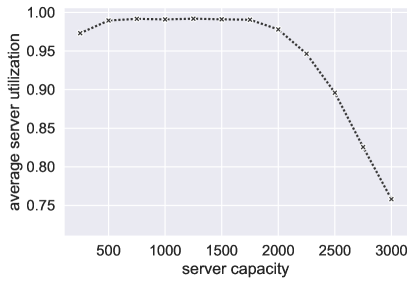
(b) Average server utilization

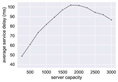
(c) Average service delay

Figure 13: Resource utilization and service delays for different server capacities in the N45 network

6.5 Discussion and remarks

From all three scenarios analyzed, we see observe that in all cases, predicting the traffic demands helps to reduce the overall number of migrations, replications and usage of the cloud. More specifically, the overprovisioning case requires in general less replications compared to the other two cases, but requires as many migrations as with the prediction case, when the network is overloaded and considerably more when the network is underloaded. Because overprovisioning does not consider the fluctuations of traffic, it can, in the best case, match the real traffic and, in the worst case, to provision excessive resources in advance, which results in using more the cloud compared to the other two cases. Placing VNFs only considering the observed traffic results in using a similar total amount of resources as with prediction, since there is no much difference in the number of replications and usage of the cloud, but it requires significantly more migrations to be able to accommodate future demands. In summary, we can say that when using traffic prediction, the number of migrations can be reduced up to 45% when there is enough available resources to allocate replicas, compared to other cases studied. This is true at expenses of using replications and cloud placements, as much as in the observed traffic case. When comparing it to the overprovisioning case, that statement remains true, but also the usage of the cloud is reduced by allocating almost up to double number of replications. However, for traffic prediction to successfully help on this problem, it requires certain amount of training periods per independent traffic demand in the network, which can result in high computational resources and computational time for larger networks.

7 Conclusions

We studied the problem of optimal placement of VNFs from an ISP point of view, when minimizing migrations and replications. We proposed a traffic forecasting model using LSTM networks and used it to place VNFs accordingly to the predicted traffic demands. We proposed an offline MILP model as well as an online greedy algorithm for the placement optimization problem. We compared three scenarios by either considering: (i) the current observed traffic demands only, (ii) overprovisioning of the 80% of every specific maximum traffic demand value had in the past, or (iii) the predicted traffic values based on history. We showed that with traffic prediction, the number of migrations can be reduced up to 45% when there is enough available resources to allocate replicas. This also results in less usage of the third-party clouds as compared to capacity overprovisioning. While overprovisioning can be valid a solution when unexpected traffic peaks appear resulting in higher usage of the cloud temporarily, traffic prediction can minimize the need for the same that by anticipating a proper placement and replication inside the network. The usage of LSTM networks, however, requires non-negligible training time and computational resources which is also something that needs to be taken into consideration.

References

- Alawe et al. [2018] Alawe, I., Ksentini, A., Hadjadj-Aoul, Y., Bertin, P., 2018. Improving traffic forecasting for 5g core network scalability: A machine learning approach. IEEE Network 32, 42–49. doi:10.1109/MNET.2018.1800104.
- Alharbi et al. [2019] Alharbi, H.A., Elgorashi, T.E., Lawey, A.Q., Elmirghani, J.M., 2019. The Impact of Inter-Virtual Machine Traffic on Energy Efficient Virtual Machines Placement. 2019 IEEE Sustainability through ICT Summit, StICT 2019 doi:10.1109/STICT.2019.8789381.
- Basta et al. [2017] Basta, A., Blenk, A., Hoffmann, K., Morper, H.J., Hoffmann, M., Kellerer, W., 2017. Towards a Cost Optimal Design for a 5G Mobile Core Network based on SDN and NFV. IEEE Transactions on Network and Service Management 4537, 1–14. doi:10.1109/TNSM.2017.2732505.
- Bulut and Ralphs [2015] Bulut, A., Ralphs, T., 2015. On the Complexity of Inverse Mixed Integer Linear Optimization. URL: https://coral.ise.lehigh.edu/~ted/files/papers/InverseMILP15.pdf.
- Carpio et al. [2017a] Carpio, F., Bziuk, W., Jukan, A., 2017a. Replication of Virtual Network Functions: Optimizing link utilization and resource costs, in: 2017 40th International Convention on Information and Communication Technology, Electronics and Microelectronics (MIPRO), Croatian Society MIPRO. doi:10.23919/MIPRO.2017.7973481.
- Carpio et al. [2017b] Carpio, F., Dhahri, S., Jukan, A., 2017b. VNF placement with replication for Load balancing in NFV networks, in: IEEE International Conference on Communications, IEEE. doi:10.1109/ICC.2017.7996515.
- Carpio et al. [2018] Carpio, F., Jukan, A., Pries, R., 2018. Balancing the Migration of Virtual Network Functions with Replications in Data Centers, in: NOMS 2018 - 2018 IEEE/IFIP Network Operations and Management Symposium, IEEE. doi:10.1109/NOMS.2018.8406275.
- Cziva et al. [2018] Cziva, R., Anagnostopoulos, C., Pezaros, D.P., 2018. Dynamic, Latency-Optimal vNF Placement at the Network Edge. Proceedings - IEEE INFOCOM 2018-April, 693–701. doi:10.1109/INFOCOM.2018.8486021.
- Ding et al. [2017] Ding, W., Yu, H., Luo, S., 2017. Enhancing the reliability of services in NFV with the cost-efficient redundancy scheme. IEEE International Conference on Communications 1. doi:10.1109/ICC.2017.7996840.
- Engelmann and Jukan [2018] Engelmann, A., Jukan, A., 2018. A Reliability Study of Parallelized VNF Chaining, in: 2018 IEEE International Conference on Communications (ICC), IEEE. pp. 2–7. doi:10.1109/ICC.2018.8422595.
- Eramo et al. [2017] Eramo, V., Miucci, E., Ammar, M., Lavacca, F.G., 2017. An Approach for Service Function Chain Routing and Virtual Function Network Instance Migration in Network Function Virtualization Architectures. IEEE/ACM Transactions on Networking doi:10.1109/TNET.2017.2668470.
- Gember-Jacobson et al. [2014] Gember-Jacobson, A., Viswanathan, R., Prakash, C., Grandl, R., Khalid, J., Das, S., Akella, A., 2014. OpenNF: Enabling Innovation in Network Function Control. SIGCOMM Comput. Commun. Rev. 44, 163–174. doi:10.1145/2740070.2626313.
- Golkarifard et al. [2021] Golkarifard, M., Chiasserini, C.F., Malandrino, F., Movaghar, A., 2021. Dynamic VNF placement, resource allocation and traffic routing in 5g. Computer Networks 188, 107830. doi:https://doi.org/10.1016/j.comnet.2021.107830.
- Huang et al. [2018] Huang, M., Liang, W., Ma, Y., Guo, S., 2018. Throughput maximization of delay-sensitive request admissions via virtualized network function placements and migrations. IEEE International Conference on Communications 2018-May. doi:10.1109/ICC.2018.8422337.
- Kim et al. [2019] Kim, H.G., Lee, D.Y., Jeong, S.Y., Choi, H., Yoo, J.H., Hong, J.W.K., 2019. Machine Learning-Based Method for Prediction of Virtual Network Function Resource Demands, in: 2019 IEEE Conference on Network Softwarization (NetSoft), IEEE. URL: https://ieeexplore.ieee.org/document/8806687, doi:10.1109/NETSOFT.2019.8806687.
- Laghrissi and Taleb [2019] Laghrissi, A., Taleb, T., 2019. A Survey on the Placement of Virtual Resources and Virtual Network Functions. IEEE Communications Surveys and Tutorials 21, 1409–1434. doi:10.1109/COMST.2018.2884835.
- Michael Till Beck, Juan Felipe Botero et al. [2016] Michael Till Beck, Juan Felipe Botero, K.S., Beck, M.T., Botero, J.F., Michael Till Beck, Juan Felipe Botero, K.S., 2016. Resilient Allocation of Service Function Chains, in: IEEE Conference on Network Function Virtualization and Software Defined Networks (NFV-SDN), IEEE. doi:10.1109/NFV-SDN.2016.7919487.
- Mijumbi et al. [2016] Mijumbi, R., Hasija, S., Davy, S., Davy, A., Jennings, B., Boutaba, R., 2016. A connectionist approach to dynamic resource management for virtualised network functions doi:10.1109/CNSM.2016.7818394.
- Mijumbi et al. [2017] Mijumbi, R., Hasija, S., Davy, S., Davy, A., Jennings, B., Boutaba, R., 2017. Topology-Aware Prediction of Virtual Network Function Resource Requirements. IEEE Transactions on Network and Service Management 14, 106–120. URL: https://ieeexplore.ieee.org/document/7849149, doi:10.1109/TNSM.2017.2666781.
- Qu et al. [2020] Qu, K., Zhuang, W., Shen, X., Li, X., Rao, J., 2020. Dynamic resource scaling for VNF over nonstationary traffic: A learning approach. IEEE Transactions on Cognitive Communications and Networking , 1–1doi:10.1109/TCCN.2020.3018157.
- Qu et al. [2017] Qu, L., Assi, C., Shaban, K., Khabbaz, M.J., 2017. A reliability-aware network service chain provisioning with delay guarantees in NFV-enabled enterprise datacenter networks. IEEE Transactions on Network and Service Management 14, 554–568. doi:10.1109/TNSM.2017.2723090.
- Rahman et al. [2018] Rahman, S., Ahmed, T., Huynh, M., Tornatore, M., Mukherjee, B., 2018. Auto-scaling VNFs using machine learning to improve QoS and reduce cost doi:10.1109/ICC.2018.8422788.
- Reddy and Rajamani [2014] Reddy, P.V.V., Rajamani, L., 2014. Virtualization overhead findings of four hypervisors in the CloudStack with SIGAR. 2014 4th World Congress on Information and Communication Technologies, WICT 2014 , 140–145doi:10.1109/WICT.2014.7077318.
- Shi et al. [2015] Shi, R., Zhang, J., Chu, W., Bao, Q., Jin, X., Gong, C., Zhu, Q., Yu, C., Rosenberg, S., 2015. MDP and Machine Learning-Based Cost-Optimization of Dynamic Resource Allocation for Network Function Virtualization, in: 2015 IEEE International Conference on Services Computing, IEEE. pp. 65–73. URL: https://ieeexplore.ieee.org/document/7207337, doi:10.1109/SCC.2015.19.
- Subramanya and Riggio [2019] Subramanya, T., Riggio, R., 2019. Machine learning-driven scaling and placement of virtual network functions at the network edges doi:10.1109/NETSOFT.2019.8806631.
- Sun et al. [2016] Sun, Q., Lu, P., Lu, W., Zhu, Z., 2016. Forecast-assisted NFV service chain deployment based on affiliation-aware vNF placement doi:10.1109/GLOCOM.2016.7841846.
- Tajiki et al. [2017] Tajiki, M.M., Salsano, S., Chiaraviglio, L., Shojafar, M., Akbari, B., 2017. Joint Energy Efficient and QoS-aware Path Allocation and VNF Placement for Service Function Chaining. IEEE Transactions on Network and Service Management PP, 1. doi:10.1109/TNSM.2018.2873225.
- Taleb et al. [2019] Taleb, T., Ksentini, A., Frangoudis, P.A., 2019. Follow-me cloud: When cloud services follow mobile users. IEEE Transactions on Cloud Computing 7, 369–382. doi:10.1109/TCC.2016.2525987.
- Tang et al. [2019] Tang, H., Zhou, D., Chen, D., 2019. Dynamic network function instance scaling based on traffic forecasting and VNF placement in operator data centers. IEEE Transactions on Parallel and Distributed Systems 30, 530–543. doi:10.1109/TPDS.2018.2867587.
- Xia et al. [2016a] Xia, J., Cai, Z., Xu, M., 2016a. Optimized Virtual Network Functions Migration for NFV. IEEE 22nd International Conference on Parallel and Distributed Systems Optimized doi:10.1109/ICPADS.2016.0053.
- Xia et al. [2016b] Xia, J., Pang, D., Cai, Z., Xu, M., Hu, G., 2016b. Reasonably Migrating Virtual Machine in NFV-Featured Networks. IEEE International Conference on Computer and Information Technology (CIT) doi:10.1109/CIT.2016.96.
- Yao et al. [2020] Yao, Y., Guo, S., Li, P., Liu, G., Zeng, Y., 2020. Forecasting assisted VNF scaling in NFV-enabled networks. Computer Networks 168, 107040. doi:10.1016/j.comnet.2019.107040.
- Yuan et al. [2020] Yuan, Q., Ji, X., Tang, H., You, W., 2020. Toward Latency-Optimal Placement and Autoscaling of Monitoring Functions in MEC. IEEE Access 8, 41649–41658. doi:10.1109/ACCESS.2020.2976858.