Uncovering patterns for adverse pregnancy outcomes with a Bayesian spatial model: Evidence from Philadelphia

Abstract

We introduce a Bayesian conditional autoregressive model for analyzing patient-specific and neighborhood risks of stillbirth and preterm birth within a city. Our fully Bayesian approach automatically learns the amount of spatial heterogeneity and spatial dependence between neighborhoods. Our model provides meaningful inferences and uncertainty quantification for both covariate effects and neighborhood risk probabilities through their posterior distributions. We apply our methodology to data from the city of Philadelphia. Using electronic health records (45,919 deliveries at hospitals within the University of Pennsylvania Health System) and United States Census Bureau data from 363 census tracts in Philadelphia, we find that both patient-level characteristics (e.g. self-identified race/ethnicity) and neighborhood-level characteristics (e.g. violent crime) are highly associated with patients’ odds of stillbirth or preterm birth. Our neighborhood risk analysis further reveals that census tracts in West Philadelphia and North Philadelphia are at highest risk of these outcomes. Specifically, neighborhoods with higher rates of women in poverty or on public assistance have greater neighborhood risk for these outcomes, while neighborhoods with higher rates of college-educated women or women in the labor force have lower risk. Our findings could be useful for targeted individual and neighborhood interventions.

1 Introduction

1.1 Background

Despite advancements in maternal health, adverse pregnancy outcomes such as stillbirth and preterm birth continue to be major public health problems. While there has been a 90 percent reduction in infant mortality over the past century [23], rates of stillbirth (i.e. fetal death at or after 20 weeks of pregnancy) have remained largely unchanged [16, 38]. For example, in 2013, a total of 23,595 stillbirths were reported in the United States (U.S.) [19]. This represents a country-wide statistic and therefore the number of stillbirths in any individual city for a given year is often very sparse.

Preterm birth (i.e. birth before 37 weeks of pregnancy) is another adverse pregnancy outcome that has gradually increased over time. The Centers for Disease Control and Prevention (CDC) estimated that in 2014, preterm birth affected one of every 10 infants in the U.S. [9]. According to the CDC, the U.S. preterm birth rate also increased from 9.57% in 2014 to 9.93% in 2017 [21].

Adverse pregnancy outcomes are significantly associated with increased risk of neonatal mortality and morbidity, adverse neuro-developmental and cognitive outcomes, and increased health care costs [27, 42]. To reduce a patient’s likelihood of experiencing an adverse pregnancy outcome, it is crucial to understand the factors that may contribute to them. Gaining insight into these risk factors can help to guide clinical interventions. Such care might entail more frequent prenatal visits, early induction of labor, or Cesarean deliveries [38].

Apart from patient-specific risk, it is also of interest to quantify the neighborhood risk of these outcomes. A neighborhood is defined as a spatial unit (e.g. a census tract) within a larger geographic area such as a city or a state. The occurrence of adverse perinatal outcomes is often geographically heterogeneous, with some areas that are more severely affected [36, 43]. Thus, some researchers have argued that it is critical to conduct location-specific analyses in order to better develop targeted intervention strategies for subpopulations at highest risk [36].

Researchers have identified environmental (or neighborhood-level) risk factors for patient-specific risk of adverse pregnancy outcomes. Several studies have suggested that neighborhood characteristics such as local exposure to pollutants, residential segregation, crime levels, and income inequality may also contribute to a patient’s risk of adverse pregnancy outcomes and other maternal outcomes such as severe maternal morbidity [15, 14, 25].

While patient-specific risk of adverse perinatal outcomes has been studied extensively, there has been comparatively less work on quantifying this risk for geographic areas. To identify higher-risk regions for preterm birth, South et al. [36] estimated the spatial density of preterm birth probabilities in Hamilton County, Ohio using spatial filtering techniques. Zahrieh et al. [43] and Zahrieh et al. [44] used Bayesian Poisson processes to discover regions with high intensities of stillbirth events in Iowa. While these researchers identified general geographic areas with elevated risk of adverse pregnancy outcomes, they did not quantify such risk for specific neighborhoods.

Targeted social policies and programs are often implemented in practice at a neighborhood level [35]. For example, city councils may designate specific neighborhoods as “priority neighborhoods” for targeted investment [35]. Recently, there has been growing interest in place-based interventions and policies for addressing health disparities [24]. Place-based interventions are approaches for improving population health within a defined geographic location, delivered at a local or regional level rather than at a national level [24]. Thus, we aim to quantify the neighborhood risks for stillbirth and preterm birth for the predetermined census tracts in a city.

1.2 Our contributions

Our main objective is to model stillbirth and preterm birth within the predefined neighborhoods of a city. We are not aware of any previous studies that have quantified the neighborhood risks for these two adverse pregnancy outcomes at the census tract level. In fitting our statistical model, we have several desiderata. First, the results should be easily interpretable to both clinicians and public health practitioners. Secondly, our findings should have the potential to guide both patient-specific and place-based interventions to reduce stillbirth and preterm rates. To this end, we develop a conditional autoregressive (CAR) logistic regression model that incorporates spatial information from adjacent neighborhoods in order to improve estimates for individual sites.

We briefly motivate the use of the CAR model (described in greater detail in Section 3.1). Since our motivating dataset (introduced in Section 2) consists of patients that are nested (and aggregated for privacy reasons) within predefined census tracts of Philadelphia, we employ a multilevel model that allows for heterogeneity between the census tracts. Moreover, we would like to account for not only spatial heterogeneity but also possible spatial dependence between the neighborhoods. A CAR model allows us to model both heterogeneity and spatial dependence through spatially correlated random effects. At the same time, a CAR logistic regression model also retains the interpretability of a typical generalized linear mixed model (GLMM), enabling one to obtain odds ratios for potential risk factors, as well as patient-specific and neighborhood risk probabilities.

We use our method to study two adverse pregnancy outcomes in Philadelphia, currently the sixth most populous city in the U.S. Philadelphia is a particularly compelling case study because it is a large urban area that has been experiencing population growth and changes to its built environment for the first time in decades [1]. While our study focuses on Philadelphia, the methods that we introduce in Section 3 can be applied to any city.

We conduct a two-part statistical analysis. In the first stage, we introduce our Bayesian CAR model for estimating patient-specific risk factors of stillbirth and preterm birth. Our CAR model accounts for spatial dependence between geographic neighbors and thus facilitates principled sharing of information across different neighborhoods. Moreover, our fully Bayesian approach automatically learns the amount of spatial autocorrelation from the data. To assess the association of patient-level and neighborhood-level risk factors with patient-specific risks of these outcomes, we propose to use a measure that we call Bayes-$p$ (originally introduced by Makowski et al. [20] as the Bayesian Probability of Direction). Rather than testing for significant effect sizes, the Bayes-$p$ quantifies how well a covariate effect can be distinguished from a null effect.

In the second stage of our analysis, we aggregate the estimates from our spatial model to predict the neighborhood probabilities for stillbirth and preterm birth. A major benefit our Bayesian model is that we can naturally quantify the uncertainty of these predicted neighborhood risk probabilities through their posterior distributions. We then cluster the individual census tracts into “lower-risk,” “moderate-risk,” and “higher-risk” neighborhoods for each outcome. This enables us to identify specific neighborhoods with elevated risk of stillbirth and preterm birth.

The rest of the paper is organized as follows. In Section 2, we describe the dataset that motivated our study. In Section 3, we introduce our modeling approaches for quantifying patient-level and neighborhood risk of adverse pregnancy outcomes. Section 4 applies our methods to a case study on stillbirth and preterm birth in Philadelphia. Section 5 concludes the paper with a discussion.

2 Motivating data

We first obtained data on patients at hospitals within the University of Pennsylvania Health System (also known as Penn Medicine) from 2010 to 2017. We used a previously developed and validated algorithm by Canelón et al. [7] to identify deliveries from Penn Medicine electronic health records (EHRs). After removing 17,305 patients with either missing values in the patient address or who lived outside of Philadelphia, our dataset contained an initial total of 46,029 deliveries at Penn Medicine hospitals between 2010 and 2017. Further exclusion criteria for our cohort are described subsequently.

Within each EHR, the following delivery outcomes were annotated: Cesarean section delivery, stillbirth, and preterm birth (each coded as either “1” or “0”). In addition, the EHRs also reported each patient’s residential address, the age of the patient at the time of delivery, binary variables for the patient’s self-reported racial/ethnic group (Hispanic, non-Hispanic White, non-Hispanic Black or non-Hispanic Asian) and a binary variable for multiple birth (e.g. twins, triplets).

The city of Philadelphia is made up of 384 census tracts determined by the U.S. Census Bureau. We matched the patients’ residential addresses to their specific longitude and latitude coordinates. Based on these coordinates, we then mapped each of the patients to one of 384 census tracts. Because some census tracts were very sparsely populated (e.g. the areas around rivers), we removed tracts that had fewer than 10 deliveries in each of the eight years or that did not share a border with any tract having at least 10 deliveries. This preprocessing procedure removed 21 census tracts and 110 observations from our dataset. Our final cohort contained $N=45{,}919$ deliveries in $n=363$ census tracts, among whom had 385 stillbirths and 2897 preterm births.

Table 1: The 19 covariates that we used in our analysis of adverse pregnancy outcomes in Philadelphia.

Patient-Level	Description
age	Age of the patient
Black	Indicator if the patient self-identifies as Black
Hispanic	Indicator if the patient self-identifies as Hispanic
Asian	Indicator if the patient self-identifies as Asian
multiple birth	Indicator if multiple babies were delivered
Neighborhood-Level	Description
proportion Asian	Proportion of neighborhood that is Asian
proportion Hispanic	Proportion of neighborhood that is Hispanic
proportion Black	Proportion of neighborhood that is Black
proportion women	Proportion of women aged 15-50
poverty	Proportion of women aged 15-50 below the poverty level
public assistance	Proportion of women aged 15-50 who received public assistance
labor force	Proportion of women aged 16-50 who were in the labor force
recent birth	Proportion of women who gave birth in the past 12 months
high school grad	Proportion of women aged 15-50 who graduated high school
college grad	Proportion of women aged 15-50 with a Bachelor’s degree
occupied housing	Total number of occupied housing units (log-transformed)
housing violation	Total number of housing violations (log-transformed)
violent crime	Total number of violent crimes (log-transformed)
nonviolent crime	Total number of nonviolent crimes (log-transformed)

Next, we augmented our dataset with neighborhood covariates based on the census tracts where each of the patients lived. Most of the neighborhood-level data was downloaded in June 2020 from https://data.census.gov/cedsci/, the U.S. Census Bureau’s online data dissemination platform. We downloaded datasets documenting racial makeup, poverty status, education level, and number of housing units for each census tract in Pennsylvania from 2010 through 2017. We also included neighborhood-level data on crime, previously analyzed by Balocchi and Jensen [1], from https://opendataphilly.org, where the Philadelphia Police Department publicly releases the location, time, and type of each reported crime in the city. For our study, we included the total number of violent crimes and nonviolent crimes from 2010 to 2017 in each of the census tracts as neighborhood-level predictors. Violent crimes included murders, rapes, robberies and aggravated assaults, whereas nonviolent crimes included burglaries, larceny/theft, motor vehicle thefts and arson.

Table 1 describes all 19 of the patient-level and neighborhood-level covariates that we included in our study. Some additional preprocessing of the data was done to ensure that there was not severe multicollinearity among the covariates. These details are provided in Appendix C.

3 Statistical methodology

3.1 Patient-specific risk analysis

Our motivating dataset from Section 2 contains geospatial data linked to Philadelphia census tracts. To account for both neighborhood heterogeneity and potential spatial autocorrelation between neighborhoods, we propose a fully Bayesian CAR model for modeling adverse pregnancy outcomes. Let $y_{ij}$ be a binary response variable, with “1” indicating if an adverse pregnancy outcome occurred for patient $j$ in the $i$th neighborhood. Suppose that we have $n$ neighborhoods and a total of $N=\sum_{i=1}^{n}m_{i}$ observations, where $m_{i}$ denotes the number of patients in the $i$th neighborhood. We assume that each $y_{ij}$ follows a conditionally independent Bernoulli distribution, that is,

$$y_{ij}\mid p_{ij}\sim\textrm{Bernoulli}(p_{ij}),\hskip 14.22636pti=1,\ldots,n,j=1,\ldots,m_{i}.$$ (1)

A standard model for estimating the $p_{ij}$’s in (1) is the mixed effects logistic regression model,

$$\log\left(\frac{p_{ij}}{1-p_{ij}}\right)=\alpha_{i}+\bm{x}_{ij}^{\top}\bm{\beta},$$ (2)

where $\bm{x}_{ij}$ is a $p$-dimensional vector that contains the $p$ covariates for the $j$th patient in neighborhood $i$, $\bm{\beta}=(\beta_{1},\dots,\beta_{p})^{\top}\in\mathbb{R}^{p}$ is a vector of unknown regression coefficients (the fixed effects), and $\alpha_{i}$ is a random effect that accounts for the variation in neighborhood $i$ that cannot be explained by the $p$ covariates.

Let $\bm{\alpha}=(\alpha_{1},\ldots,\alpha_{n})^{\top}$ denote the vector of neighborhood-specific random effects. In order to incorporate the neighborhood information in our spatial analysis, we employ a CAR prior on $\bm{\alpha}$ [2, 17, 18]. The CAR model is a Gaussian Markov random field which induces spatial dependence through an adjacency matrix for the areal units, which in our case study, are the census tracts of Philadelphia. We use the proper CAR formulation of Leroux et al. [18], which defines the distribution of each $\alpha_{i}$, given the other entries $\bm{\alpha}_{-i}$, as a normal distribution centered at a weighted average of a global mean $\alpha_{0}$ and the $\alpha_{j}$’s from neighborhoods that share a border with $\alpha_{i}$. That is,

$$\alpha_{i}\mid\bm{\alpha}_{-i},\alpha_{0},\tau_{\alpha},\rho\sim\mathcal{N}\left(\frac{\rho\sum_{j}w_{ij}\alpha_{j}+(1-\rho)\alpha_{0}}{\rho\sum_{j}w_{ij}+(1-\rho)},\frac{\tau_{\alpha}^{2}}{\rho\sum_{j}w_{ij}+(1-\rho)}\right),$$ (3)

where the $w_{ij}$’s are adjacency weights that are equal to one if the neighborhoods $i$ and $j$ share a border and equal to zero otherwise. The autocorrelation parameter $\rho\in[0,1)$ represents the strength of spatial correlation between the components of $\bm{\alpha}$, with larger values of $\rho$ corresponding to stronger influence of bordering neighborhoods.

We collect the adjacency weights $w_{ij}$ into an adjacency matrix $\bm{W}$, constructed using shape files from the U.S. Census Bureau to determine which of the census tracts share a border. The joint distribution of $\bm{\alpha}$ is then uniquely determined by the set of conditional distributions defined in (3) and can be written more compactly as

$$\bm{\alpha}\mid\alpha_{0},\tau_{\alpha},\rho\sim\mathcal{N}\left(\alpha_{0}\cdot\bm{1},\tau_{\alpha}^{2}\bm{\Sigma}_{\rm CAR}\right),$$ (4)

where $\bm{1}$ is a $n$-dimensional vector of all ones, $\bm{\Sigma}^{-1}_{\rm CAR}=\rho(\bm{D}_{\bm{W}}-\bm{W})+(1-\rho)\bm{I}_{n}$, and $\bm{D}_{\bm{W}}-\bm{W}$ is the Laplacian matrix based on the neighborhood adjacency matrix $\bm{W}$.[1] In our spatial logistic model, we use (4) as the prior for $\bm{\alpha}$ in (2). If $\rho=0$ in (4), then our model reduces to a GLMM with independent (non-spatially correlated) neighborhood random effects.

There are various hypothesis tests to determine the degree of spatial autocorrelation in a CAR model (4). For example, Moran’s $I$ statistic [26] has widely been used in practice to test for the presence of significant spatial autocorrelation. As an alternative to testing if $\rho=0$ (or more generally, if $\rho=\rho_{0}$ for some fixed $\rho_{0}\in[0,1)$), a Bayesian approach can be used to adaptively learn the amount of spatial autocorrelation from the data and to model the implicit uncertainty about $\rho$. To this end, we endow the autocorrelation parameter $\rho$ in (4) with a standard uniform prior,

$$\rho\sim\mathcal{U}(0,1).$$ (5)

The posterior distribution $p(\rho\mid\bm{y})$ can be used to assess the strength of spatial autocorrelation (see e.g. Figure 1). If there is weak or negligible autocorrelation, then the posterior for $\rho$ will concentrate most of its posterior probability near zero. Moreover, since $\rho$ is sampled in each iteration of our Markov chain Monte Carlo (MCMC) algorithm and subsequently used to sample the model parameters $(\bm{\alpha},\bm{\beta})$, we obtain posterior samples of $(\bm{\alpha},\bm{\beta})$ based on different values of $\rho$. In this sense, the prior on $\rho$ (5) also facilitates model averaging over varying degrees of spatial autocorrelation.

We further endow the grand mean $\alpha_{0}$ and the global scale parameter $\tau_{\alpha}$ in (4) with weakly informative priors,

$$\alpha_{0}\sim\mathcal{N}(0,100),~{}~{}\tau_{\alpha}\sim\mathcal{C}^{+}(0,1),$$ (6)

where $\mathcal{C}^{+}(0,1)$ denotes a half-Cauchy distribution. To complete our prior specification, we place a weakly informative prior on the fixed effects $\bm{\beta}$ in (2) as

$$\bm{\beta}\mid\bm{b}_{0},\tau_{\beta}\sim\mathcal{N}(\bm{b}_{0},\tau_{\beta}^{2}\bm{I}_{p}),~{}~{}\bm{b}_{0}\sim\mathcal{N}(\bm{0}_{p},100\cdot\bm{I}_{p}),~{}~{}\tau_{\beta}\sim\mathcal{C}^{+}(0,1).$$ (7)

The spatial logistic regression model (2) under the priors (4)-(7) can be implemented using Markov chain Monte Carlo (MCMC). The complete MCMC algorithm is provided in Appendix B.

To conduct inference about the covariate effects, we propose using the Bayes-$p$ measure, originally introduced as the Probability of Direction by Makowski et al. [20]. The Bayes-$p$ for the $j$th covariate is the posterior probability that the corresponding regression coefficient $\beta_{j}$ has the sign of its posterior median, or the maximum posterior probability that $\beta_{j}$ is either less than zero or greater than zero. That is,

$$\text{Bayes-}p=\max\left\{P(\beta_{j}>0\mid\bm{y}),P(\beta_{j}<0\mid\bm{y})\right\}.$$ (8)

The Bayes-$p$ (8) is a posterior probability quantifying how well the posterior distribution can be distinguished from a null effect. It should be stressed that the Bayes-$p$ does not pertain to the hypothesis testing framework and is quite different from a frequentist $p$-value. A smaller p-value indicates a higher level of statistical significance, whereas a larger Bayes-$p$ corresponds to a predictor that is more highly associated with the outcome. Some illustrations and motivations for using the Bayes-$p$ are provided in Appendix A.

3.2 Neighborhood risk analysis

The approaches that we introduced in Section 3.1 allow us to quantify the patient-specific risk for stillbirth and preterm birth. However, we also aim to quantify the neighborhood risk probabilities of these outcomes for each of the $n=363$ census tracts of Philadelphia. The patient-specific risk analysis in Section 3.1 is based on conditional comparisons among different risk factors. In other words, the effects of each risk factor are determined conditionally on the other covariates in the model. As a result, high correlations between covariates might mask the true associations between some of the predictor variables and the outcome of interest. Contrastingly, our neighborhood risk analysis allows for marginal comparisons of the risk factors between different neighborhoods and clusters of neighborhoods (see Table 3, for example).

First, we define the risk probability $p_{ij}$ for patient $j$ living in the $i$th census tract as $p_{ij}=e^{\theta_{ij}}/(1+e^{\theta_{ij}})$, where $\theta_{ij}$ is the log-odds, $\theta_{ij}=\alpha_{i}+\bm{x}_{ij}^{\top}\bm{\beta}$, and $\alpha_{i}$ and $\bm{\beta}$ are as in (2). Based on all $m_{i}$ individuals’ risk probabilities in the $i$th neighborhood, we define the neighborhood risk probability $p_{i}$ for the $i$th neighborhood as

$$p_{i}=\frac{1}{m_{i}}\sum_{j=1}^{m_{i}}p_{ij}.$$ (9)

We can approximate the posterior distributions of the predicted neighborhood probabilities $p(p_{i}\mid\bm{y}),i=1,\ldots,n$, using the MCMC samples of $(\bm{\alpha},\bm{\beta})$ from our CAR model in Section 3.1. These posterior distributions can naturally quantify the uncertainty of these neighborhood risk probabilities (9).

In epidemiology, it is common to develop different risk categories for community health. For example, the CDC has categorized all of the U.S. counties’ community levels of coronavirus disease 2019 (COVID-19) as either “low,” “medium,” or “high.” To aid in the interpretability of our results for neighborhood risk of stillbirth and preterm birth, we similarly stratify the census tracts of Philadelphia into three risk categories. Specifically, we take the posterior means $\widehat{p}_{i}$ of $p(p_{i}\mid\bm{y}),i=1,\ldots,n$ and cluster the predicted $\widehat{p}_{i}$’s into three groups using $k$-means clustering: “lower-risk,” “moderate-risk,” and “higher-risk” neighborhoods. The cluster assignments for the $n$ neighborhoods are then subsequently used to form the aggregate risk posteriors $p(p_{LR}\mid\bm{y}),p(p_{MR}\mid\bm{y})$, and $p(p_{HR}\mid\bm{y})$, where $p_{LR}$, $p_{MR}$, and $p_{HR}$ denote the predicted probabilities for the lower-risk, moderate-risk, and higher-risk clusters of neighborhoods respectively. For cluster $c\in\{LR,MR,HR\}$, let $n_{c}$ denote the number of neighborhoods in that cluster. The neighborhood cluster risk is defined as

$$p_{c}=\frac{1}{n_{c}}\sum_{i\in c}p_{i},$$ (10)

where $p_{i}$ is the $i$th neighborhood’s risk probability (9).

It should be stressed that we do not claim that there are only three “true” clusters of neighborhood risks of stillbirth or preterm birth. Rather, our approach aims to easily extract neighborhood patterns in Philadelphia that are interpretable to maternal health practitioners (see Table 3 and bottom two panels of Figure 3). A similar approach to ours was used by Byrnes et al. [6]. It is certainly possible to stratify the neighborhoods into more than three risk categories. However, for our dataset, we found that the three aggregate risk posterior densities $p(p_{LR}|y)$, $p(p_{MR}|y)$, and $p(p_{HR}|y)$ were fairly well-separated (see Figure 4). Moreover, limiting the number of risk categories to three allowed us to easily detect spatial patterns in neighborhood risk, as we describe in Section 4.3.

4 Results from our case study of Philadelphia

4.1 Model fitting and validation

We now apply the modeling approaches described in Sections 3.1 and 3.2 to the study of stillbirths and preterm births in Philadelphia. For the CAR model that we introduced in Section 3.1, we ran two MCMC chains for a total of 5500 iterations each, using the MCMC algorithm described in Appendix B. For each chain, we removed the first 500 iterations as burn-in. We also thinned our chains every 10 iterations, leaving us with a total of 1000 samples from the two chains. In Appendix E, we report MCMC diagnostics (trace plots, autocorrelation plots, and MCMC standard errors) to confirm that the number of iterations we used was sufficient to achieve convergence and that our thinned samples were not too correlated. Before fitting our models, we also standardized all the continuous variables to lie on the same scale. Our model’s estimates of the regression coefficients were then transformed back to their original scale for our final analysis.

We used the first six years of data from 2010 to 2016 to perform the patient-specific risk analysis in Section 4.2. The remaining year of data 2017 was used for model validation and for predicting the neighborhood risk probabilities in Section 4.3. We refer to these two datasets as the training set (years 2010 to 2016) and the validation set (year 2017), respectively. The reason that we estimated the neighborhood risk probabilities on a completely out-of-sample validation set was to avoid overfitting to the training set.

All of our analysis was done using the R programming language [32]. In Appendix E, we report all of the R packages that were used to conduct our analyses and produce the results in this article.

4.2 Results for patient-specific risk analysis

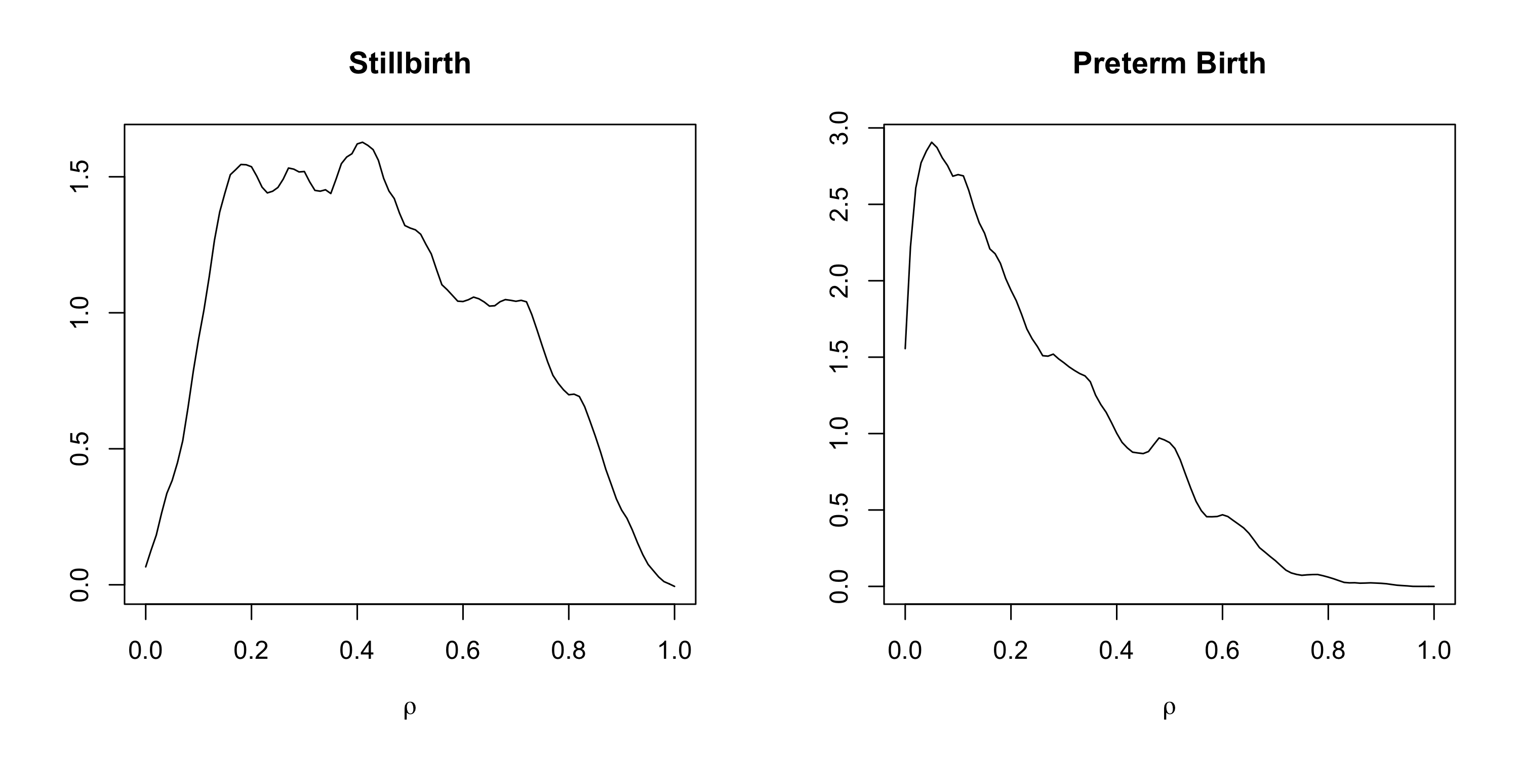
Figure 1: Plots of the posterior densities for autocorrelation parameter $\rho$ for stillbirth (left panel) and preterm birth (right panel) under the CAR model.

We first examined the posterior densities for the autocorrelation parameter $\rho$ under the CAR model introduced in Section 3.1. Figure 1 shows the plots of the marginal posteriors $p(\rho\mid\bm{y})$ for stillbirth (left panel) and preterm birth (right panel). For stillbirth, we observe that the majority of the posterior mass for $\rho$ was between 0.2 and 0.6, with non-negligible mass greater than 0.8. Figure 1 suggests that the unexplained variation for stillbirth is spatially autocorrelated and that some unmeasured, spatially correlated covariates might help to explain the variation in stillbirth. On the other hand, for preterm birth, most of the posterior mass for $\rho$ was between 0 and 0.2, but there was still some posterior mass on values greater than 0.2. This suggests that there is weaker – but possibly still non-negligible – autocorrelation in the unexplained variation for preterm birth than stillbirth.

To further validate the appropriateness of our spatial model, we used two different Bayesian information criteria to compare the model fit of the CAR model to a non-spatial Bayesian mixed effects model. These results are reported in Appendix D.1 and confirm that the CAR model provides a better fit to our data than a purely non-spatial Bayesian mixed effects model.

Table 2: Posterior mean odds ratios (OR) and Bayes-$p$ measures for stillbirth and preterm birth under the CAR model.

	Stillbirth		Preterm birth
	OR	Bayes-$p$	OR	Bayes-$p$
Patient-level
age	1.01	0.79	1.00	0.95
Black	2.23	1.00	1.55	1.00
Hispanic	1.61	1.00	0.94	0.79
Asian	0.97	0.58	1.12	0.84
multiple birth	4.17	1.00	10.56	1.00
Neighborhood-level
proportion Asian	1.01	0.58	0.90	0.58
proportion Hispanic	0.45	0.95	0.72	1.00
proportion Black	0.61	0.95	0.92	0.74
proportion women	0.24	0.89	1.88	1.00
poverty	3.92	1.00	0.87	0.63
public assistance	0.49	0.84	0.89	0.58
labor force	1.25	0.58	0.49	1.00
recent birth	1.40	0.74	1.48	0.79
high school grad	1.16	0.58	2.63	1.00
college grad	0.50	0.89	0.74	0.79
occupied housing	0.99	0.53	0.93	0.68
housing violation	0.88	0.84	0.99	0.68
violent crime	1.59	1.00	1.16	1.00
nonviolent crime	0.75	1.00	0.97	0.63

In Table 2, we report the posterior mean odds ratio (OR) and the Bayes-$p$ (8) for all 19 covariates in our CAR model. Recall that the Bayes-$p$ allows for direct comparison of the strength of association between different covariate effects and the outcome of interest, with a larger Bayes-$p$ value indicating a stronger association. We also plot the 95% posterior credible intervals of the log-odds ratio for these 19 covariates in Figure 2.

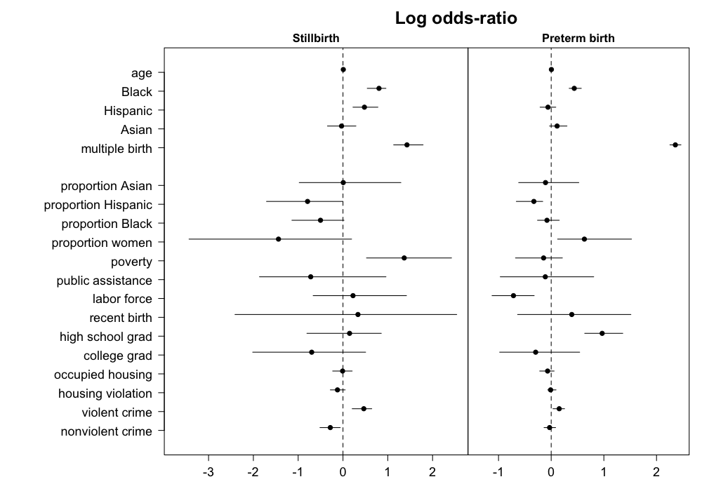
Figure 2: Posterior mean and 95% credible intervals of the log odd-ratios for the 19 covariates under our CAR model. The results are shown for both stillbirth (left) and preterm birth (right).

We found that self-identifying as Black or Hispanic and experiencing multiple birth were the patient-level risk factors that were the most highly associated with patient-specific risk for stillbirth (Bayes-$p$=1). Among the neighborhood-level risk factors for stillbirth, the proportion of Hispanic and Black residents, the proportion of women living below the poverty line, and the number of both violent and nonviolent crimes were the most highly associated with a patient’s stillbirth risk (Bayes-$p$ $\geq 0.95$). On the other hand, the patient-level risk factors most highly associated with patient-specific risk of preterm birth were the patient’s age, whether or not they self-identified as Black, and whether or not they gave multiple birth (Bayes-$p$ $\geq 0.95$). Meanwhile, the neighborhood-level risk factors most highly associated with preterm birth were the number of violent crimes, the neighborhood proportion of Hispanic residents, and the neighborhood proportions of women who were aged 15 to 50, who were in the labor force, or who had graduated high school (Bayes-$p$ $=1$).

We highlight a few specific findings that may warrant further research and action from medical and public health professionals. After controlling for other variables, it appears as though patients who self-identify as Black are at much higher risk of stillbirth (OR=2.23) and preterm birth (OR=1.55), compared to White patients. Self-identified Hispanics are also at much higher risk of stillbirth (OR=1.61) than White patients. Finally, patients experiencing multiple birth are at much higher risk of stillbirth (OR=4.17) and preterm birth (OR=10.56) than those giving birth to only one baby. These findings suggest that both maternal racial/ethnic group and multiple birth play an important role in determining a patient’s likelihood of experiencing stillbirth or preterm birth.

Among the neighborhood-level risk factors, we found that after controlling for other variables, an increase in neighborhood violent crime was highly associated with greater risk of both stillbirth (OR=1.59) and preterm birth (OR=1.16). Increased neighborhood poverty also led to much higher patient-specific risk of stillbirth (OR=3.92), while an increase in proportion of women who graduated from high school led to much higher patient-specific risk of preterm birth (OR=2.63). Finally, an increase in the percentage of women in the labor force was associated with much lower patient-specific risk of preterm birth (OR=0.49). Our findings suggest that place-based policies and investments to decrease violent crime, alleviate poverty, and increase in the number of women in the labor force may reduce patient-specific risk of stillbirth or preterm birth for women living in these neighborhoods.

4.3 Results for neighborhood risk analysis

In this section, we discuss the main findings from our neighborhood analysis (described in Section 3.2). The top two panels of Figure 3 plot the posterior means of the predicted neighborhood risk probabilities (9) for stillbirth and preterm birth. For stillbirth (top left panel of Figure 3), the neighborhoods with the lowest risk probabilities tended to be concentrated in Center City and areas immediately adjacent to Center City (such as Fishtown and Fairmount to the north and Bella Vista and Southwest Center City to the south) and in Northwest Philadelphia. Additionally, some small pockets of census tracts with lower risk can be found in Northeast Philadelphia and West Philadelphia. The census tracts with the highest risk of stillbirth were in North Philadelphia (such as North Philadelphia West), West Philadelphia (such as Cathedral Park, West Parkside, Mantua and Kingsessing) and South Philadelphia (such as Grays Ferry and West Passyunk).

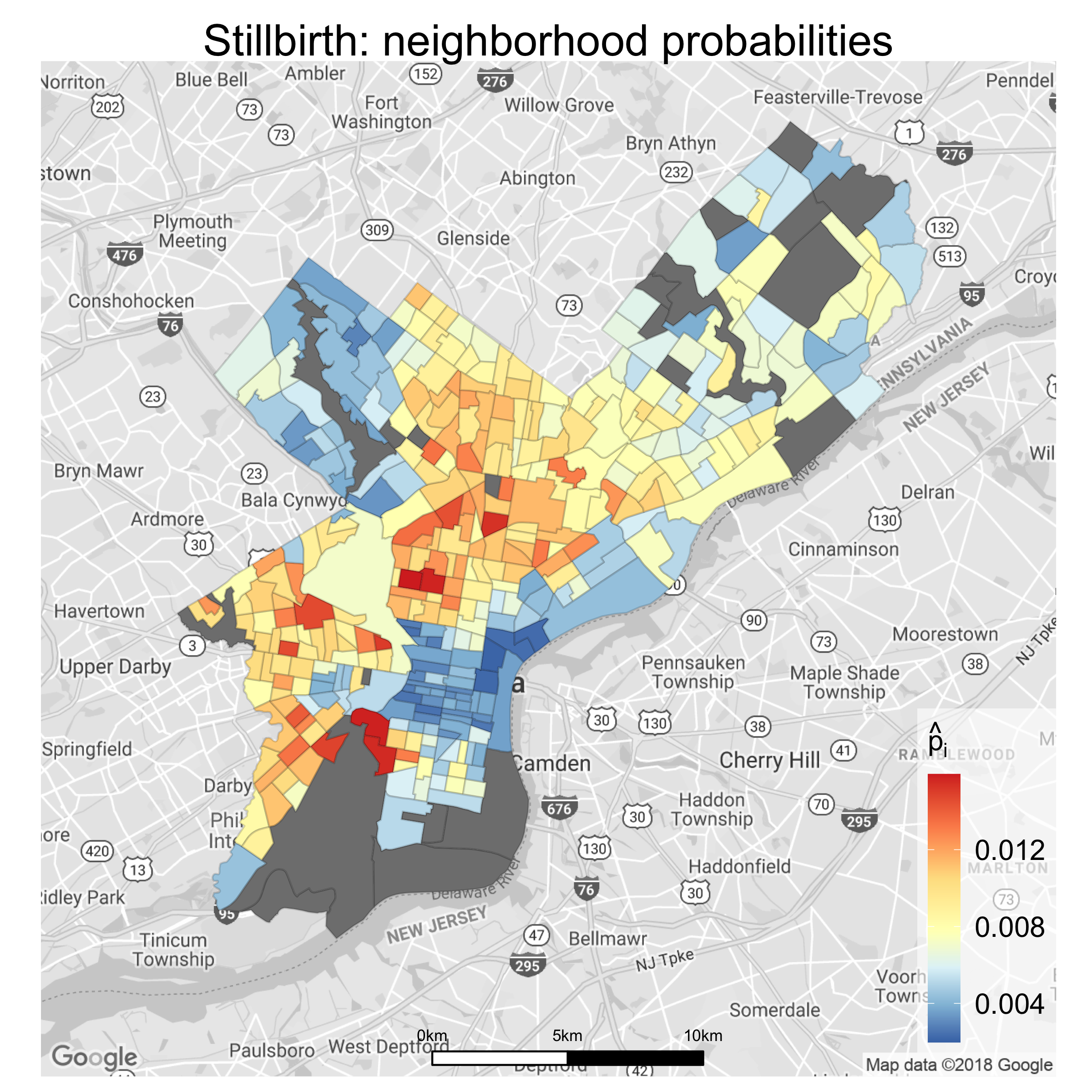
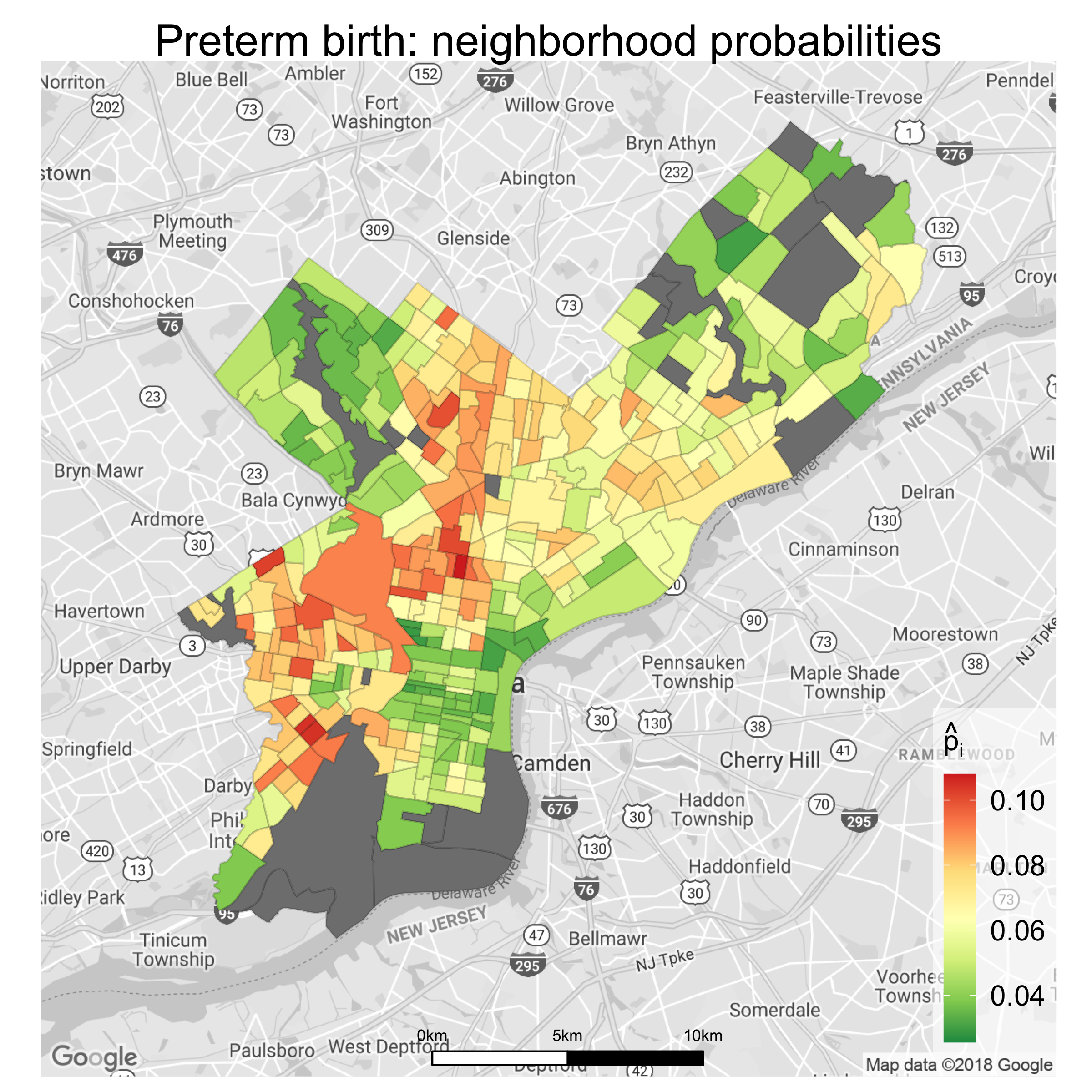
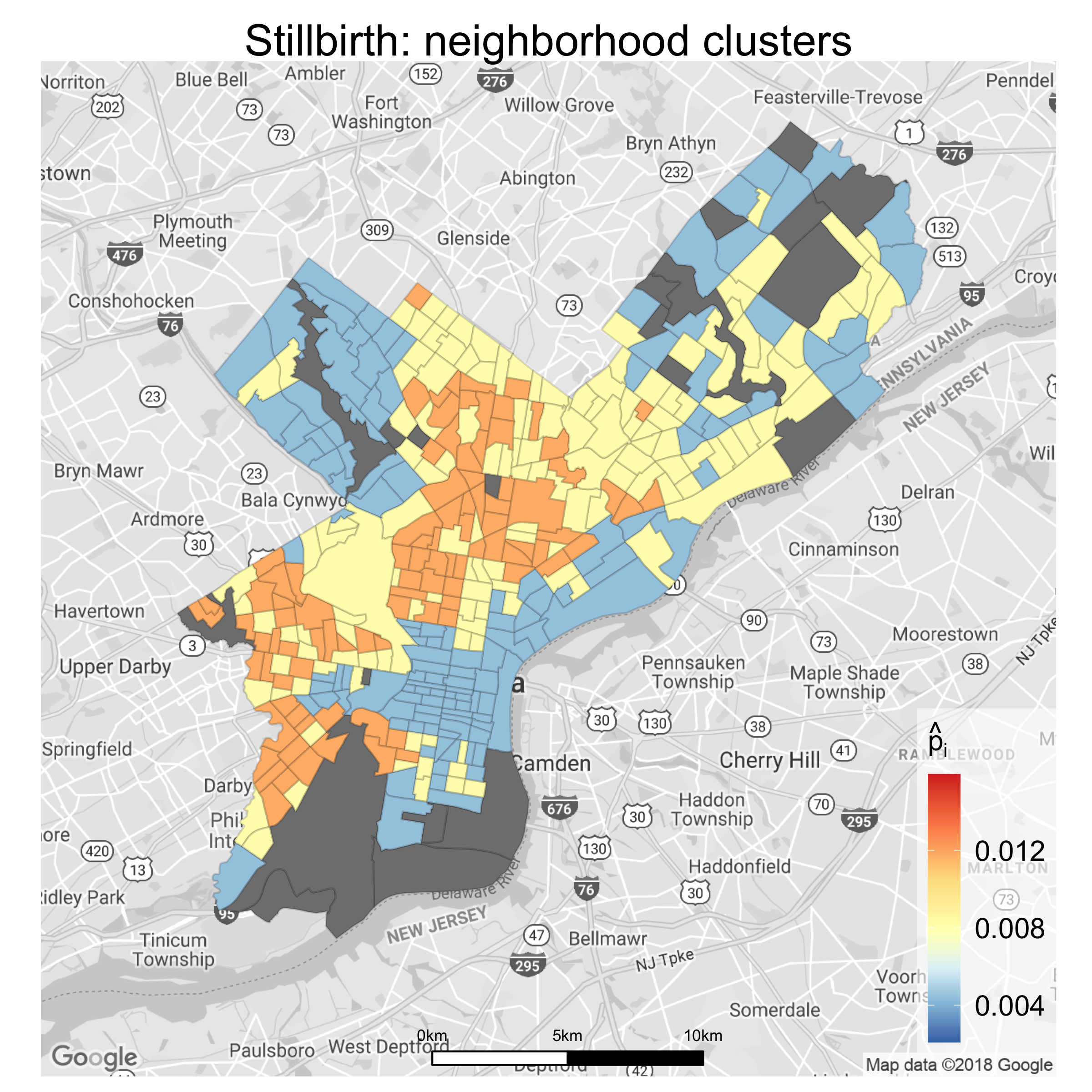
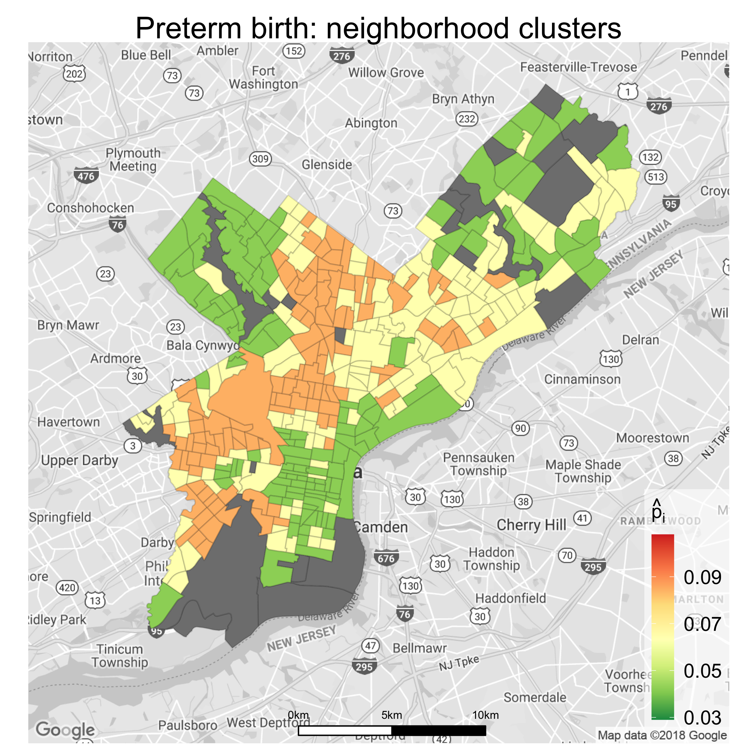
Figure 3: Top two panels: Maps of the predicted (posterior mean) neighborhood probabilities of having an adverse pregnancy outcome for stillbirth (left panel) and preterm birth (right panel). Bottom two panels: Maps of the clusters of lower-risk, moderate-risk and higher-risk neighborhoods for stillbirth (left panel) and preterm birth (right panel). The orange clusters are the higher risk neighborhoods and the light yellow clusters are the moderate risk clusters. The neighborhoods shown in gray are the very sparsely populated census tracts that were excluded from our analysis.

The top right panel of Figure 3 plots the posterior means of the predicted neighborhood probabilities (9) for preterm birth. Similar to stillbirth, we found that most of the areas with lower risk of preterm birth were concentrated in Center City and its surrounding neighborhoods and in Northwest Philadelphia, with some small pockets in Northeast Philadelphia and West Philadelphia. Moreover, we also found several census tracts with higher risk of preterm birth in North Philadelphia (especially in North Philadelphia West, Upper North Philadelphia and East Germantown) and in West Philadelphia (especially in Kingsessing, Cathedral Park and West Parkside).

Clustering the neighborhoods into “lower-risk,” “moderate-risk,” or “higher-risk” categories allowed us to more easily visualize the spatial distribution of neighborhood risks for stillbirth and preterm birth in Philadelphia. In particular, the census tracts in the higher or moderate risk clusters also tended to be spatially clustered. The bottom two panels of Figure 3 plot the cluster assignments for all 363 census tracts. These maps confirm that most of the higher-risk neighborhoods for stillbirth and preterm birth were concentrated in North Philadelphia and West Philadelphia. In addition, North Philadelphia and Northeast Philadelphia also contained many moderate-risk clusters.Table 3 shows the number of neighborhoods in each risk category. 95 neighborhoods were categorized as “higher-risk” for stillbirth, and 112 neighborhoods were categorized as “higher-risk” for preterm birth.

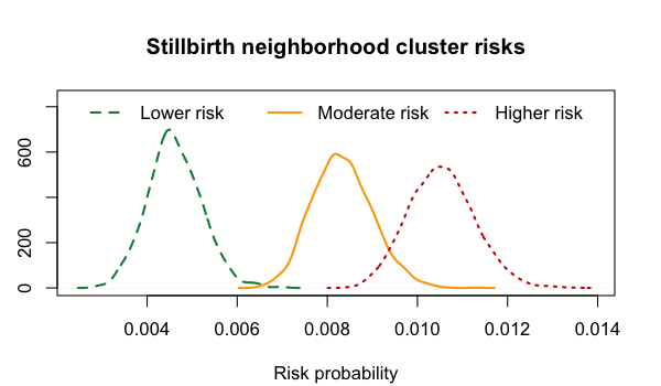
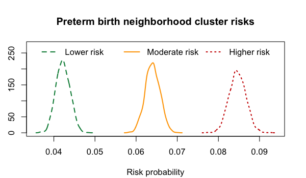
Figure 4: The neighborhood cluster risk posteriors for stillbirth (left panel) and preterm birth (right panel). The $95\%$ credible intervals for the clusters probabilities are respectively $(0.0034,0.0058)$, $(0.0071,0.0097)$ and $(0.0092,0.0120)$ for stillbirth and $(0.039,0.045)$, $(0.060,0.067)$ and $(0.081,0.088)$ for preterm birth.

Figure 4 plots the neighborhood cluster risk posterior distributions $p(p_{LR}\mid\bm{y})$, $p(p_{MR}\mid\bm{y})$, and $p(p_{HR}\mid\bm{y})$ for the three risk categories. We see that the cluster risks (10) for the higher-risk group were on average more than double those for the lower-risk group. In particular, the posterior mean risks for lower-risk neighborhoods were 0.0044 for stillbirth and 0.0422 for preterm birth. These risks more than doubled to 0.0118 for stillbirth and 0.0847 for preterm birth in the high-risk neighborhoods. Moreover, there was no overlap between the 95% credible intervals for $p(p_{LR}\mid\bm{y})$ and $p(p_{MR}\mid\bm{y})$ for either stillbirth or preterm birth. This suggests that our model was able to separate the neighborhoods with elevated (moderate or higher) risk of stillbirth and preterm birth.

Previous research has found that neighborhoods in North and West Philadelphia tend to have poorer health outcomes than other neighborhoods in Philadelphia. According to the Philadelphia Health Rankings website https://phillyhealthrankings.org/, residents in North and West Philadelphia are burdened with lower lifespans on average and higher rates of high cholesterol, hypertension, diabetes, and heart disease than Philadelphia as a whole. Our findings on the elevated neighborhood risk of stillbirth and preterm birth in North and West Philadelphia seem to be consistent with previous findings on other poor health outcomes in these same neighborhoods. We note that the website Philadelphia Health Rankings has not tracked the neighborhood incidences for either stillbirth or preterm birth.

Finally, we used our predicted cluster risk probabilities to study the discrepancies in neighborhood characteristics. For each of the neighborhood-level covariates, we computed the mean covariate value within each cluster and regressed these on the clusters’ risk probabilities. Table 3 summarizes our main results. The “Up/down” column in Table 3 indicates the sign of the slope of the regression if the slope was found to be significantly different from zero. More detailed results from this analysis are given in Appendix D.2.

From Table 3, we see that neighborhoods with higher risk of stillbirth and preterm birth tended to have higher proportions of Black residents, higher proportions of women living below the poverty line and on public assistance, and higher numbers of housing violations and violent crimes. Meanwhile, neighborhoods with lower risk of these outcomes tended to have higher proportions of Asian residents and higher proportions of women who were in the labor force or who had graduated from college. Our findings suggest that place-based policies to reduce poverty and violent crime may reduce neighborhood risk of stillbirth and preterm birth. In addition, expanding educational opportunities and labor force participation among women may also lower neighborhood risk of stillbirth and preterm birth.

Table 3: Predicted (posterior mean) neighborhood cluster risk probability ($\widehat{p}_{c}$), number of neighborhoods ($n_{c}$), and average neighborhood characteristics for the clusters of lower, moderate and higher-risk neighborhoods. Plus and minus signs indicate the direction of each of the neighborhood characteristics (i.e. whether they tend to increase or decrease with higher risk), if they are determined to be significantly different from zero.

	Stillbirth				Preterm birth
	Lower	Moderate	Higher	Up/	Lower	Moderate	Higher	Up/
	risk	risk	risk	down	risk	risk	risk	down
$\widehat{p}_{c}$	0.44%	0.81%	1.18%		4.22%	6.40%	8.47%
$n_{c}$	126	142	95		119	132	112
proportion Asian	0.09	0.07	0.03	–	0.09	0.07	0.03	–
proportion Hispanic	0.07	0.14	0.14	+	0.08	0.18	0.08
proportion Black	0.16	0.50	0.78	+	0.16	0.43	0.80	+
proportion women	0.30	0.28	0.28	–	0.29	0.28	0.29
poverty	0.17	0.28	0.41	+	0.17	0.29	0.37	+
public assistance	0.03	0.08	0.11	+	0.03	0.07	0.12	+
labor force	0.77	0.68	0.63	–	0.77	0.68	0.64	–
recent birth	0.04	0.05	0.06	+	0.04	0.06	0.06	+
high school grad	0.17	0.30	0.35	+	0.16	0.30	0.35	+
college grad	0.29	0.13	0.07	–	0.31	0.13	0.07	–
occupied housing	7.26	7.28	7.31		7.31	7.29	7.24
housing violation	3.87	4.45	5.00	+	3.75	4.51	4.93	+
violent crime	3.91	4.54	5.08	+	3.81	4.62	4.97	+
nonviolent crime	4.64	4.54	4.73		4.52	4.68	4.67	+

While we have done a comparative study of different clusters of neighborhoods in this section, our model also facilitates comparisons between specific individual neighborhoods that may be of interest. In Appendix D.3, we present pairwise neighborhood risk comparisons for four representative pairs of neighborhoods. These pairs of neighborhoods have very different values for at least one of the covariates in Table 3. For example, in one of the pairs, the first neighborhood has a very low proportion of college-educated women ($\approx 0.00$), while the second neighborhood has a fairly high proportion of college-educated women (0.71). The posterior mean risk for stillbirth in the first neighborhood is about 3.7 times that for the second neighborhood. It is interesting to see how the neighborhood risk changes between individual neighborhoods that have very different neighborhood characteristics. Comparisons between more than two neighborhoods can also be similarly done.

5 Discussion

We have presented an important application of a Bayesian CAR model to the study of stillbirth and preterm birth. Our methods were applied to the city of Philadelphia. We used a rich EHR dataset of 45,919 deliveries at Penn Medicine hospitals from 2010 to 2017, augmented with spatially varying neighborhood data from the U.S. Census Bureau and other government agencies. Our fully Bayesian approach accounts for neighborhood heterogeneity and automatically learns the amount of spatial autocorrelation between neighborhoods from the data. Instead of assessing statistical significance using posterior credible intervals, we used the Bayes-$p$ (8) to assess how well the effects of patient-specific risk factors could be distinguished from a null effect. To analyze the neighborhood risks in Philadelphia, we aggregated the estimates from our CAR model to estimate the predicted risk probabilities for both individual census tracts and clusters of census tracts.

We found that both patient-level and neighborhood-level risk factors were highly associated with patient-specific risk of stillbirth and preterm birth (see Table 2). In particular, maternal racial/ethnic group and multiple birth were found to be highly associated with increased risk of both of these outcomes. These results may be useful for developing patient-specific clinical interventions for higher-risk patients [38]. Previous research has linked neighborhood exposure to violent crime and small for gestational age infants, with the key finding being that across all racial/ethnic groups, there was a negative association between economic disadvantage and birth weight [22]. Our findings support this prior work while building upon it. Namely, we found that neighborhood-level violent crime was also highly associated with increased risk of two other important maternal health outcomes: stillbirth and preterm birth. Moreover, our results confirm previous research’s findings on the relationship between poverty and higher risk of stillbirth [12]. These results could potentially guide public policies to reduce neighborhood stressors that may be triggering these adverse fetal outcomes.

Going further than patient-level risk, our models have also enabled the development of measures of neighborhood risk assessment. We are able to group neighborhoods into lower, moderate, and higher risk for stillbirth and preterm birth and provide meaningful uncertainty measures for these clusters’ risk probabilities (see Figure 4). These neighborhood risks and assignments can enable place-based public health interventions to target communities that may have lower access to health care for a variety of reasons.

Our model detected a clear spatial pattern for neighborhood risk of stillbirth and preterm in Philadelphia. Neighborhoods in West Philadelphia and North Philadelphia were identified as being at highest risk for preterm birth and stillbirth (see Figure 3). In particular, our analysis revealed that higher-risk neighborhoods tended to have lower rates of women who had completed a college education or who were in the labor force. Higher-risk neighborhoods also tended to have higher rates of women who were living below the poverty line or who were on public assistance (see Table 3). Since we assessed the marginal comparisons of the risk factors in our neighborhood risk analysis, this seemingly contradictory result is explained by the collinearity between poverty and public assistance. However, when we inspect the effect of public assistance in the joint (and conditional) analysis that models patient-specific risk (see Table 2), we find that conditional on poverty, public assistance does not seem to have an effect on the risk for stillbirth or preterm birth.

These findings are important, especially since some prior work found a protective effect of public assistance against COVID-19 in the city of Philadelphia [5], whereas our findings suggest that public assistance may not have a similar protective effect against stillbirth or preterm birth. On the other hand, improved access to educational and employment opportunities might reduce the risk of these outcomes. Overall, this underscores the importance of studying neighborhood-level factors and their contributions to specific health outcomes of interest, since the relationship between a neighborhood characteristic and disease risk may vary depending on the outcome.

Software and data availability

All methods were implemented in the statistical environment R. Due to patient privacy concerns, we do not have permission to release or make the Penn Medicine data publicly available. However, code to implement our models and simulated synthetic data to run these scripts are available at https://github.com/cecilia-balocchi/geospatial-adverse-pregnancy.

Appendix A Justification for the Bayes-$p$

In epidemiological studies, it is customary to use either p-values or confidence intervals of the regression coefficients to determine the statistical significance of potential risk factors. However, final conclusions can be highly sensitive to the choice of p-value significance cutoff or confidence interval percentiles, and it may be preferable to use a quantitative measure for variable association that is more agnostic. This motivates us to use the Bayes-$p$ (8) to conduct inference about the effect sizes, instead of posterior credible intervals.

Recall that the Bayes-$p$ for the $j$th covariate,

$$\textrm{Bayes-$p$}=\max\left\{P(\beta_{j}>0\mid\bm{y}),P(\beta_{j}<0\mid\bm{y})\right\},$$

quantifies how much of a coefficient’s posterior mass differs from zero. A higher Bayes-$p$ for a variable indicates that it is more highly associated with the outcome. For example, a predictor whose posterior has a 90% probability of being less than zero will be more strongly associated with the outcome than a predictor whose posterior is centered and symmetric around zero. In practice, the Bayes-$p$ can be calculated using the MCMC samples for $\beta_{j}$.

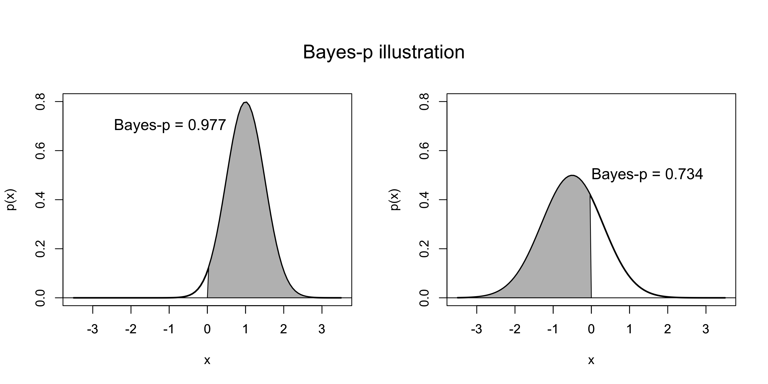
Figure 5: Graphical illustration of the Bayes-$p$ measure, computed on two Gaussian distributions $N(\mu,\sigma^{2})$, with the area shaded in gray corresponding to Bayes-$p$ for each distribution. In the left panel, $\mu=1,\sigma=0.5$, and in the right panel, $\mu=-0.5,\sigma=0.8$.

Figure 5 illustrates two examples of the Bayes-$p$ measure. In the left panel of Figure 5, the 95% credible interval is $(0.02,1.98)$ (suggesting statistical significance), while the 99% credible interval is $(-0.29,2.29)$ (suggesting an insignificant association between exposure and outcome). This demonstrates that the choice of $\alpha\in(0,1)$ in our $100(1-\alpha)\%$ posterior credible intervals can strongly influence our conclusions.

Contrastingly, the Bayes-$p$ does not depend on any threshold $\alpha$. Instead, it quantifies directly how well a covariate effect size $\beta_{j}$ can be distinguished from a null effect. In addition, posterior credible intervals do not allow for direct comparison of the effects of potential risk factors. On the other hand, the Bayes-$p$ permits comparisons between the effects of different risk factors (with a higher Bayes-$p$ indicating a stronger association with the outcome).

Appendix B MCMC algorithm

To fit our CAR model from Section 3.1, we sample from the posterior distribution with MCMC. We use a Gibbs sampler to iteratively sample from the full conditional posteriors, together with the data augmentation strategy using Pólya-Gamma latent variables proposed by Polson et al. [30]. Using the notation from Polson et al. [30], we say that a random variable $X$ is distributed from a Pólya-Gamma with parameters $b>0$ and $c\in\mathcal{R}$ if

$$X\overset{D}{=}\frac{1}{2\pi^{2}}\sum_{k=1}^{\infty}\frac{g_{k}}{(k-1/2)^{2}+c^{2}/(4\pi^{2})},$$

where $g_{k}\sim\textrm{Ga}(b,1)$, and we denote $X\sim PG(b,c)$.

As shown in Polson et al. [30], if $y_{i}\sim\text{Bernoulli}(\theta_{i})$ and $\log(\theta_{i}/(1-\theta_{i}))=\mathbf{x}_{i}^{\top}\bm{\beta}$ with $\bm{\beta}\sim\mathcal{N}(\bm{b},\bm{B})$, we can sample

$$\omega_{i}\mid\bm{\beta} \sim PG(1,\mathbf{x}_{i}^{\top}\bm{\beta}),$$

$$\bm{\beta}\mid\bm{y},\bm{\omega} \sim\mathcal{N}(\bm{m}_{\omega},\bm{V}_{\omega}),$$

with $\bm{V}_{\omega}=\left(\bm{X}^{\top}\bm{\Omega}\bm{X}+\bm{B}^{-1}\right)^{-1}$ and $\bm{m}_{\omega}=\bm{V}_{\omega}\left(\bm{X}^{\top}\bm{\Omega}\bm{\tilde{y}}+\bm{B}^{-1}\bm{b}\right)$, where $\bm{\Omega}=\text{diag}(\omega_{i})$ and $\tilde{y}_{i}=(y_{i}-0.5)/\omega_{i}$.

To adapt this sampling scheme to our model, we can write $\alpha_{i}+\mathbf{x}_{ij}^{\top}\bm{\beta}=\bm{z}_{ij}^{\top}\bm{\alpha}+\mathbf{x}_{ij}^{\top}\bm{\beta}$, where $\bm{z}_{ij}$ is a $n$-dimensional vector with all entries equal to 0, except for the $j$th entry which is equal to 1. Then the full conditional for our model can be written as

$$\omega_{ij}\mid\bm{\alpha},\bm{\beta} \sim PG(1,\alpha_{i}+\mathbf{x}_{ij}^{\top}\bm{\beta}),$$

$$\bm{\alpha}\mid\bm{y},\bm{\beta},\bm{\omega},\tau_{\alpha}^{2} \sim\mathcal{N}\left(\bm{V}_{\alpha}\left(\bm{Z}^{\top}\bm{\Omega}(\bm{\tilde{y}}-\bm{X}\bm{\beta})+\tau_{\alpha}^{-2}\bm{\Sigma}^{-1}_{\bm{\alpha}}\bm{1}\alpha_{0}\right),\bm{V}_{\alpha}^{-1}\right),$$

$$\bm{\beta}\mid\bm{y},\bm{\alpha},\bm{\omega},\tau_{\beta}^{2} \sim\mathcal{N}\left(\bm{V}_{\beta}\left(\bm{X}^{\top}\bm{\Omega}(\bm{\tilde{y}}-\bm{Z}\bm{\alpha})+\tau_{\beta}^{-2}\bm{b}_{0}\right),\bm{V}_{\beta}^{-1}\right),$$

where $\bm{Z}$ is the $N\times n$ matrix of $\bm{z}_{ij}$, $\bm{V}_{\alpha}=\bm{Z}^{\top}\bm{\Omega}\bm{Z}+\tau_{\alpha}^{-2}\bm{\Sigma}^{-1}_{\bm{\alpha}}$, $\bm{V}_{\beta}=\bm{X}^{\top}\bm{\Omega}\bm{X}+\tau_{\beta}^{-2}\bm{I}$. Moreover, $\bm{\Sigma}^{-1}_{\bm{\alpha}}$ denotes the prior covariance matrix of $\bm{\alpha}$, which is equal to $\bm{\Sigma}^{-1}_{\rm CAR}$ under model (4).

Under the CAR prior for $\bm{\alpha}$, we also need to sample the correlation parameter $\rho$. Note that this parameter affects the precision matrix of $\bm{\alpha}$, and its conditional distribution is given by

$$p(\rho\mid\textrm{rest})=p(\rho\mid\bm{\alpha},\alpha_{0},\tau_{\alpha}^{2})\propto|\bm{\Sigma}^{-1}_{\bm{\alpha}}(\rho)|^{1/2}\exp\left(-\frac{1}{2\tau_{\alpha}^{2}}(\bm{\alpha}-\alpha_{0}\bm{1})^{\top}\bm{\Sigma}^{-1}_{\bm{\alpha}}(\rho)(\bm{\alpha}-\alpha_{0}\bm{1})\right).$$

We sample from this distribution using a Metropolis Hastings-within Gibbs-step, with proposal density $g(\rho^{*}\mid\rho_{t})={\rm Beta}(\xi\cdot\rho_{t}/(1-\rho_{t}),\xi)$. This ensures that the mean is equal to $\rho_{t}$, and we choose $\xi=5$ so that $g(\rho^{\star}\mid\rho_{t}$) has small variance.

Assuming a half-Cauchy prior on $\tau_{\alpha}$ and on $\tau_{\beta}$, i.e. $p(\tau_{\alpha})\propto(\tau_{\alpha}^{2}+s_{\alpha}^{2})^{-1}$ and $p(\tau_{\beta})\propto(\tau_{\beta}^{2}+s_{\beta}^{2})^{-1}$, their conditional posterior distributions can be written as follows:

$$p(\tau_{\alpha}\mid\bm{\alpha},\alpha_{0}) \propto(\tau_{\alpha}^{2}+s_{\alpha}^{2})^{-1}\tau_{\alpha}^{n}\exp\left(-\frac{1}{\tau_{\alpha}^{2}}(\bm{\alpha}-\alpha_{0}\bm{1})^{\top}\bm{\Sigma}_{\alpha}^{-1}(\bm{\alpha}-\alpha_{0}\bm{1})/2\right),$$

$$p(\tau_{\beta}\mid\bm{\beta},\beta_{0}) \propto(\tau_{\beta}^{2}+s_{\beta}^{2})^{-1}\tau_{\beta}^{p}\exp\left(-\frac{1}{\tau_{\beta}^{2}}\sum_{k=1}^{p}(\beta_{k}-b_{0,k})^{2}/2\right).$$

To sample from these posterior distributions, we use a Metropolis-Hastings (MH) step, with a carefully designed proposal distribution. In general, given a random variable distributed according to $p(x)\propto(x^{2}+s^{2})^{-1}x^{-2\alpha}\exp(-\beta/x^{2})$, consider the following proposal distribution, $q(x)=x^{-2\alpha-1}\exp(-\beta/x^{2})$; note that $x\sim q$ is equivalent to $x^{2}\sim IG(\alpha,\beta)$. Moreover, if $\alpha$ and $\beta$ are carefully chosen, the acceptance ratio for the MH steps simplifies considerably:

$$a(x\to\tilde{x})=\frac{(x^{2}+s^{2})}{(\tilde{x}^{2}+s^{2})}\frac{\tilde{x}}{x}.$$

Thus, to sample $\tau_{\alpha}$ from its posterior, we simply need to generate from an inverse gamma distribution with parameters $\alpha=n/2$ and $\beta=(\bm{\alpha}-\alpha_{0}\bm{1})^{\top}\bm{\Sigma}_{\alpha}^{-1}(\bm{\alpha}-\alpha_{0}\bm{1})/2$, consider its square root as proposed value and compute the acceptance $a(\tau_{\alpha}\to\tilde{\tau}_{\alpha})$. Similarly, for $\tau_{\beta}$ we follow the same steps using $\alpha=p/2$ and $\beta=\sum_{k=1}^{p}(\beta_{k}-b_{0,k})^{2}/2$.

Moreover, the full conditional for the remaining parameters are standard:

$$\alpha_{0}\mid\bm{\alpha},\tau_{\alpha}^{2} \sim\mathcal{N}\left(\frac{\sum_{i=1}^{n}\alpha_{i}/\tau_{\alpha}^{2}}{1/\tau_{\alpha}^{2}+1/100},\frac{1}{1/\tau_{\alpha}^{2}+1/100}\right),$$

$$\bm{b}_{0}\mid\bm{\beta},\tau_{\beta}^{2} \sim\mathcal{N}\left(\frac{\bm{\beta}/\tau_{\beta}^{2}}{1/\tau_{\beta}^{2}+1/100},\frac{1}{1/\tau_{\beta}^{2}+1/100}\bm{I}_{p}\right).$$

Appendix C Additional data information

In Section 2, we described the data used for our analysis of adverse pregnancy outcomes in Philadelphia. While the patient-level data from Penn Medicine EHRs is not publicly available, the neighborhood-level data were downloaded from https://data.census.gov/cedsci/ and from https://opendataphilly.org. In Table 4, we describe the precise data source for each covariate. In addition, we describe some additional preprocessing of the dataset below.

Table 4: Sources and data files for neighborhood-level covariates used in our analysis. ACS refers to the American Community Survey.

Neighborhood-level covariate	Source	Data File
Proportion of each census tract that identifies as Asian Alone	ACS	B01001D
Proportion of each census tract that identifies as Black or African-American	ACS	B01001B
Proportion of each census tract that identifies as Hispanic or Latinx	ACS	B01001I
Proportion of each census tract that identifies as White Alone	ACS	B01001A
Proportion of women aged 15-50 years in each census tract	ACS	S1301
Proportion of women aged 15-50 years in each census tract below 100 percent poverty level	ACS	S1301
Proportion of women aged 15-50 years in each census tract that received public assistance income in the past 12 months	ACS	S1301
Proportion of women aged 16-50 years in each census tract that are in the labor force	ACS	S1301
Proportion of women aged 15-50 years in each census tract who had a birth in the past 12 months	ACS	B13016
Proportion of women aged 15-50 years in each census tract that graduated high school (including equivalency)	ACS	S1301
Proportion of women aged 15-50 years in each census tract that have a Bachelor’s degree	ACS	S1301
Number of occupied housing units in each census tract	ACS	S2502
Housing Violations	OpenDataPhilly
Violent Crime Rate	OpenDataPhilly
Non-Violent Crime Rate	OpenDataPhilly

In our dataset of $N=45{,}919$ deliveries, we initially included an indicator variable for whether the patient self-identified as White (White) and the neighborhood proportion of those identifying as White (proportion White) as covariates in our model. However, when we included both of these covariates, the variance inflation factors (VIF) for White and proportion White were greater than 9.5. The VIF was also greater than 9.5 for the individual and neighborhood-level race factors in Table 1 (i.e. Black, Hispanic, Asian, proportion Asian, proportion Hispanic, and proportion Black), indicating the presence of significant multicollinearity among all of the race variables [28]. The reason for this was because in the majority of cases, we could deduce the values for White and proportion White if the other variables were known. For example, if we observed Black = Hispanic = Asian = 0, then the patient typically identified as White (i.e. White = 1). On the other hand, if one of the non-White patient-level race variables in Table 1 was equal to one, then we could infer that typically the patient’s individual race was not White (i.e. White=0).

The neighborhood proportion of White residents could also often be determined by taking $\texttt{proportion White}\approx 1-(\texttt{proportion Asian}+\texttt{proportion Hispanic}+\texttt{proportion Black})$, since the proportions of Philadelphia residents identifying as Native American, Pacific Islander, Alaskan Native or Native Hawaiian were very small and therefore excluded from our analyses. Once we removed the variables White and proportion White, the VIFs for all patient-level and neighborhood-level covariates were below 9.5, indicating much less severe multicollinearity among the remaining covariates Neter et al. [28].

Appendix D Additional results

D.1 Assessing the appropriateness of a spatial model

In Section 3.1, we argued that employing a CAR model (4) with a uniform prior $\mathcal{U}(0,1)$ on the autocorrelation parameter $\rho$ allowed us to adaptively learn the degree of spatial autocorrelation between neighborhoods and model the implicit uncertainty in $\rho$. This makes it a potentially more appealing than simply employing a Bayesian mixed effects model with independent random effects for the neighborhoods (i.e. $\rho$ fixed a priori as $\rho=0$ in (4)).

Figure 1 suggests that there was moderate spatial autocorrelation for stillbirth and weak spatial autocorrelation for preterm birth. However, in order to further investigate the appropriateness of a CAR model for our data, we also compared the fit of our CAR model (4) to a Bayesian model with independent random effects (i.e. $\rho$ fixed a priori as $\rho=0$ in (4)). We compared these two models on the real dataset (described in Section 2) using two separate Bayesian model selection criteria: the Deviance Information Criterion (DIC) of Spiegelhalter et al. [37] and the Watanabe-Akaike information criterion (WAIC) of Watanabe and Opper [40].

For an unknown parameter $\bm{\theta}$, the deviance is $D(\bm{\theta})=-2\log p(\bm{y}|\bm{\theta})$, where $p(\bm{y}|\bm{\theta})$ is the likelihood for the respective model. The DIC is given by $D(\bar{\bm{\theta}})+2p_{D}$ where the first term is the deviance evaluated at the posterior mean of $\bm{\theta}$, and $p_{D}=\overline{D(\bm{\theta})}-D(\bar{\bm{\theta}})$ is the effective number of model parameters where $\overline{D(\bm{\theta})}=E_{\bm{\theta}|\bm{y}}[D(\bm{\theta})]$ is the posterior mean deviance. The DIC rewards better fitting models through the first term and penalizes more complex models through the second term. The model with the smallest overall DIC value is preferred.

As an alternative to DIC, one can also consider the WAIC. The WAIC is given by $\textrm{WAIC}=-2\log\overline{p(\bm{y}|\bm{\theta})}+2p_{W}$ where $\overline{p(\bm{y}|\bm{\theta})}$ is the posterior predictive density of the observed data, and $p_{W}=\sum_{i,j}\textrm{Var}[\log p(y_{ij}|\bm{\theta})|\bm{y}]$, as recommended in Gelman et al. [10]. Compared to DIC, WAIC considers the predictive density averaged over the posterior distribution, instead of conditioning on a point estimate, resulting in an approach more in line with the Bayesian framework.

Let $\bm{\theta}=(\bm{\alpha},\bm{\beta})$. For the mixed effects logistic regression model (2), the likelihood is defined as $p(\bm{y}|\bm{\theta})=\prod_{i,j}p(y_{ij}|\bm{\theta})=\prod_{i,j}\left[p_{ij}(\bm{\theta})^{y_{ij}}(1-p_{ij}(\bm{\theta}))^{1-y_{ij}}\right],$ where $p_{ij}(\bm{\theta})=\exp(\alpha_{i}+\mathbf{x}_{ij}^{\top}\bm{\beta})/(\exp(\alpha_{i}+\mathbf{x}_{ij}^{\top}\bm{\beta})+1)$. In practice, we estimate $\bar{\bm{\theta}}$, $\overline{D(\bm{\theta})}$, $\overline{p(\bm{y}|\bm{\theta})}$ and $\textrm{Var}[\log p(y_{ij}|\bm{\theta})|\bm{y}]$ using MCMC samples from the algorithm described in Appendix B and then compute the DIC as $\textrm{DIC}=2\overline{D(\bm{\theta})}-D(\overline{\bm{\theta}})$ and the WAIC as $\textrm{WAIC}=-2\log\overline{p(\bm{y}|\bm{\theta})}+2\sum_{i,j}\textrm{Var}[\log p(y_{ij}|\bm{\theta})|\bm{y}]$. The model with the smallest DIC or WAIC provides the best model fit.

We fit the CAR and the independent random effects (indRE) to our training set and computed the DIC and WAIC using the validation set. The training and validation data are described in Section 4.1. Our results are presented in Table 5. We see that the CAR model has a smaller DIC and WAIC for both stillbirth and preterm birth. This suggests that the CAR model is more appropriate to use than the indRE model for this particular dataset. However, we reiterate that by putting a prior on $\rho$ in (4), we are capturing the inherent uncertainty in the spatial autocorrelation $\rho$. Therefore, we believe that the CAR model is still appropriate to use for areal data even when spatial autocorrelation is fairly negligible. In this case, the CAR model would still be able to adaptively learn the absence of strong autocorrelation, and the posterior mass for $\rho$ would be concentrated near zero.

Table 5: Comparisons of model fit for the CAR model vs. the independent random effects (indeRE) model using DIC and WAIC.

	Stillbirth		Preterm birth
	CAR	indRE	CAR	indRE
DIC	380.1	382.3	883.8	885.1
WAIC	380.3	382.5	883.8	885.2

D.2 Additional results for the neighborhood risk analysis

In Section 4.3, we presented a comparative analysis of the neighborhood characteristics between “lower-risk,” “moderate-risk,” and “higher-risk” clusters of neighborhoods that we found. Here, we regressed the mean neighborhood covariate values of each cluster on the posterior mean predicted risk probabilities for each cluster. The main results of this analysis were reported in Table 3. In Tables 6 and 7, we report more detailed results for stillbirth and preterm birth respectively. In the rightmost columns of Tables 6 and 7, we report the magnitudes of the estimated slope and the p-values from the simple linear regression models that we fit.

Table 6: Average neighborhood characteristics of the clusters of lower-risk, moderate-risk, and higher-risk neighborhoods for stillbirth are given in the first three columns. Results from three-way ANOVA tests and simple linear regression on the cluster risk probabilities are reported in the last two columns.

Stillbirth	Lower risk	Moderate risk	Higher risk	ANOVA		Slopes
$\hat{p}$	0.44%	0.81%	1.18%
	$\bar{x}_{j}$	$\bar{x}_{j}$	$\bar{x}_{j}$	F-value	p-value	$\beta$	p-value
proportion Asian	0.0862	0.0673	0.0266	16.3005	0.0000	-7.9247	0.0000
proportion Hispanic	0.0729	0.1441	0.1367	6.3663	0.0019	9.2469	0.0042
proportion Black	0.1606	0.5012	0.7776	144.7190	0.0000	84.1930	0.0000
proportion women	0.2974	0.2808	0.2762	5.0093	0.0071	-2.9566	0.0030
poverty	0.1659	0.2828	0.4120	102.9180	0.0000	33.2907	0.0000
public assistance	0.0328	0.0824	0.1130	58.5833	0.0000	11.0247	0.0000
labor force	0.7675	0.6820	0.6320	48.3316	0.0000	-18.6495	0.0000
recent birth	0.0394	0.0546	0.0617	18.8219	0.0000	3.0859	0.0000
high school grad	0.1690	0.3006	0.3521	110.1243	0.0000	25.4390	0.0000
college grad	0.2945	0.1303	0.0699	195.1799	0.0000	-31.2494	0.0000
occupied housing	7.2564	7.2836	7.3087	0.4074	0.6657	7.1142	0.3668
housing violation	3.8695	4.4477	5.0005	52.0092	0.0000	153.6266	0.0000
violent crime	3.9053	4.5420	5.0788	95.5258	0.0000	159.9585	0.0000
nonviolent crime	4.6378	4.5386	4.7254	3.0265	0.0497	9.7213	0.3644

In addition to these simple linear regressions, we also performed one-way analysis of variance (ANOVA) tests to test whether the mean neighborhood covariate values differed significantly across lower-risk, moderate-risk, and higher-risk groups of neighborhoods. We report the $F$-statistics and p-values from these ANOVA tests in the second rightmost columns of Tables 6 and 7. We see that there is agreement between the ANOVA tests and the linear regression models that we fit. Namely, if the ANOVA test determined that there was no significant difference between the lower-risk, moderate-risk, and higher-risk groups for a particular neighborhood characteristic (occupied housing and nonviolent crime for stillbirth; and proportion women, occupied housing, and housing violations for preterm birth), then the linear regression slope for that neighborhood characteristic was also not significantly different from zero.

Table 7: Average neighborhood characteristics of the clusters of lower-risk, moderate-risk, and higher-risk neighborhoods for preterm birth are given in the first three columns. Results from three-way ANOVA tests and simple linear regression on the cluster risk probabilities are reported in the last two columns.

Preterm	Lower risk	Moderate risk	Higher risk	ANOVA		Slopes
$\hat{p}$	4.22%	6.40%	8.47%
	$\bar{x}_{j}$	$\bar{x}_{j}$	$\bar{x}_{j}$	F-value	p-value	$\beta$	p-value
proportion Asian	0.0870	0.0694	0.0306	15.8705	0.0000	-1.3188	0.0000
proportion Hispanic	0.0802	0.1794	0.0840	13.6561	0.0000	0.1865	0.7340
proportion Black	0.1603	0.4263	0.8029	184.8069	0.0000	15.0807	0.0000
proportion women	0.2904	0.2794	0.2870	1.3702	0.2554	-0.0905	0.5923
poverty	0.1671	0.2935	0.3712	67.5253	0.0000	4.8321	0.0000
public assistance	0.0309	0.0749	0.1163	70.4655	0.0000	2.0140	0.0000
labor force	0.7705	0.6797	0.6444	44.4952	0.0000	-2.9971	0.0000
recent birth	0.0412	0.0556	0.0567	10.8672	0.0000	0.3721	0.0000
high school grad	0.1561	0.2999	0.3505	141.7264	0.0000	4.6243	0.0000
college grad	0.3080	0.1338	0.0709	257.6153	0.0000	-5.6392	0.0000
occupied housing	7.3053	7.2916	7.2418	0.6980	0.4982	-1.4778	0.2668
housing violation	3.7539	4.5071	4.9331	65.1284	0.0000	27.9321	0.0000
violent crime	3.8085	4.6217	4.9665	108.7947	0.0000	27.5036	0.0000
nonviolent crime	4.5159	4.6786	4.6676	2.9690	0.0526	3.6579	0.0428

D.3 Pairwise comparisons of neighborhood risks

In Section 4.3, we provided a visualization of the posterior mean predicted probabilities of an adverse outcome for each neighborhood (Figure 3). However, to better compare how the collective set of covariates affects the neighborhood risk, we compare several pairs of neighborhoods which differ for one or more neighborhood-level covariates. So far, we have presented results in terms of the odds ratio (OR) for each predictor, but this can be misleading since the covariates cannot be artificially changed keeping the others fixed. Thus, we now study how neighborhood-level covariates jointly change by considering four representative pairs of neighborhoods.

It is important not to consider the predictors in isolation (as they are often correlated), but to analyze the differences between two neighborhoods for all their covariates jointly. For a predictor of interest, consider a pair of neighborhoods that display the minimum and maximum values for such predictors. One can then visualize how the other covariates change and how all of them affect the change in neighborhood risk of an adverse pregnancy outcome.

Table 8: Comparison of risk probabilities and relative odds ratio for pairs of neighborhoods that differ for a specific neighborhood-level characteristic: “proportion Black” for neighborhoods $B_{\min}$ and $B_{\max}$, “labor force” for neighborhoods $L_{\min}$ and $L_{\max}$, “college grad” for neighborhoods $C_{\min}$ and $C_{\max}$, and “violent crime” for neighborhoods $V_{\min}$ and $V_{\max}$.

	$B_{\min}$	$B_{\max}$	$L_{\min}$	$L_{\max}$	$C_{\min}$	$C_{\max}$	$V_{\min}$	$V_{\max}$
Stillbirth
$\hat{p}$	0.38%	1.1%	0.71%	0.22%	1.41%	0.38%	0.29%	0.92%
$\rm{OR}_{2}/\rm{OR}_{1}$	291.67%		31.4%		26.76%		321.1%
Preterm birth
$\hat{p}$	3.44%	8.49%	9.15%	4.52%	7.56%	3.44%	3.4%	8.03%
$\rm{OR}_{2}/\rm{OR}_{1}$	260.71%		47.04%		43.51%		247.85%
proportion Asian	0.11	0.00	0.43	0.04	0.01	0.09	0.01	0.02
proportion Hispanic	0.01	0.00	0.02	0.06	0.00	0.12	0.04	0.18
proportion Black	0.00	1.00	0.17	0.07	0.98	0.02	0.00	0.63
proportion women	0.39	0.23	0.59	0.36	0.25	0.30	0.20	0.31
poverty	0.23	0.32	0.95	0.08	0.48	0.22	0.00	0.35
public assistance	0.01	0.12	0.00	0.00	0.02	0.01	0.00	0.19
labor force	0.78	0.54	0.12	0.98	0.60	0.75	0.63	0.68
recent birth	0.01	0.02	0.00	0.00	0.07	0.09	0.07	0.06
high school grad	0.00	0.17	0.03	0.02	0.29	0.00	0.04	0.39
college grad	0.56	0.03	0.03	0.54	0.00	0.71	0.38	0.03
occupied housing	7.64	6.99	5.33	7.62	7.44	7.72	6.21	7.84
housing violation	3.56	5.21	1.82	4.09	5.36	4.45	0.48	5.93
violent crime	4.43	4.82	4.57	4.63	5.05	4.44	0.48	6.23
nonviolent crime	5.66	4.17	5.63	5.77	5.04	5.65	3.14	5.74

Table 8 reports the comparisons for four representative pairs of neighborhoods, displaying their covariates and the neighborhood OR for an adverse pregnancy outcome. The $i$th neighborhood’s OR can be computed as $\exp(\theta_{i})$, where $\theta_{i}=\alpha_{i}+\bm{x}_{ij}^{\top}\bm{\beta}$ is the neighborhood log-odds ratio. These pairs of neighborhoods were chosen to maximize the discrepancy in the proportion of Black inhabitants ($B_{\min}$ and $B_{\max}$), the proportion of women in the labor force ($L_{\min}$ and $L_{\max}$), the proportion of women who graduated from college ($C_{\min}$ and $C_{\max}$) and the level of violent crime ($V_{\min}$ and $V_{\max}$).

It is interesting to notice that the pairs of neighborhoods do not differ only in the level of the chosen predictor. For example, $B_{\min}$ and $B_{\max}$ have very different proportions of women who are college graduates. $L_{\min}$ and $L_{\max}$ also differ in the proportion of women below the poverty line, while $V_{\min}$ and $V_{\max}$ have very different levels of housing violations. The last four rows of the table compare the predicted risk of stillbirth and preterm birth for each pair of neighborhoods, along with the fraction of the two odds ratios.

D.4 Spatial distribution of estimated random effects

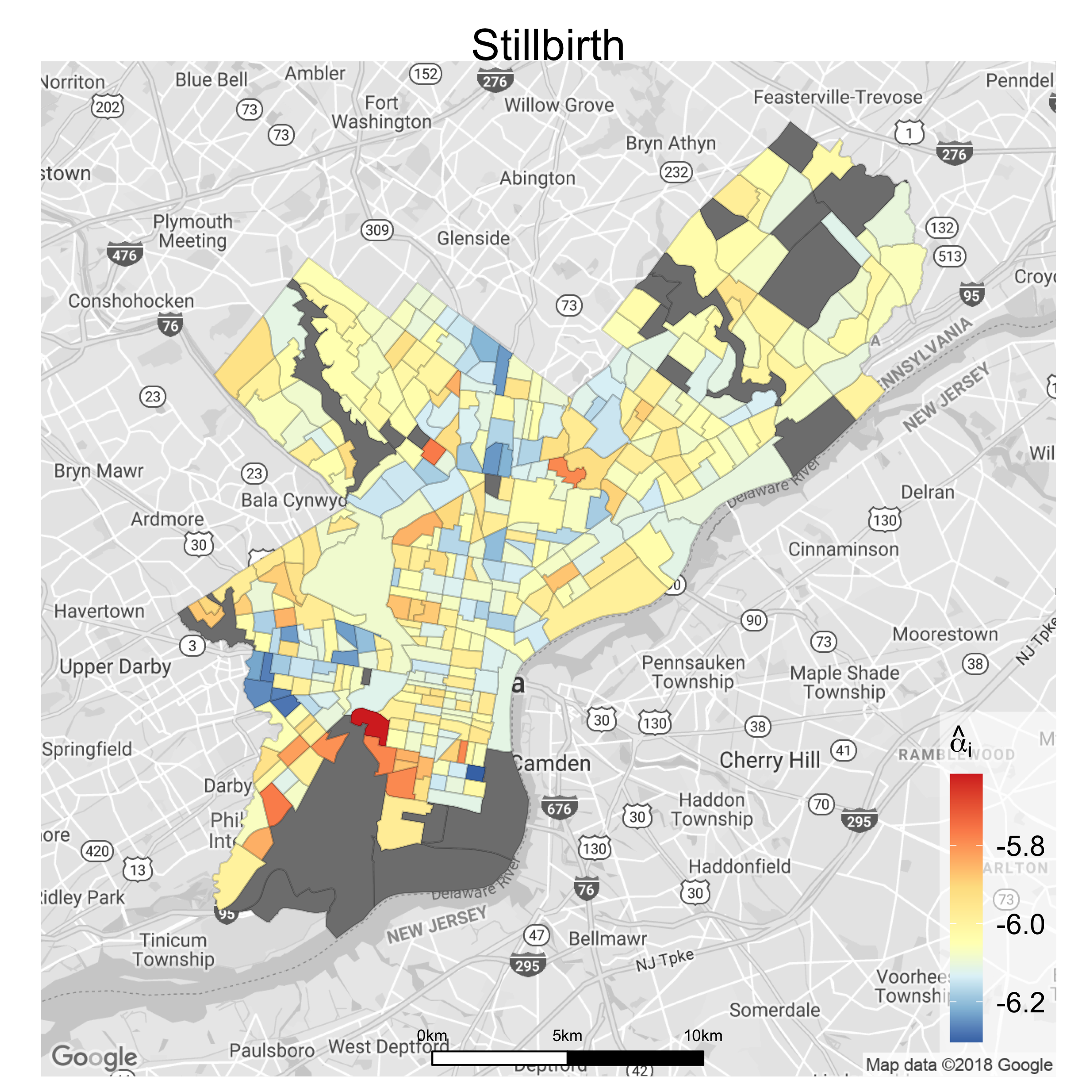
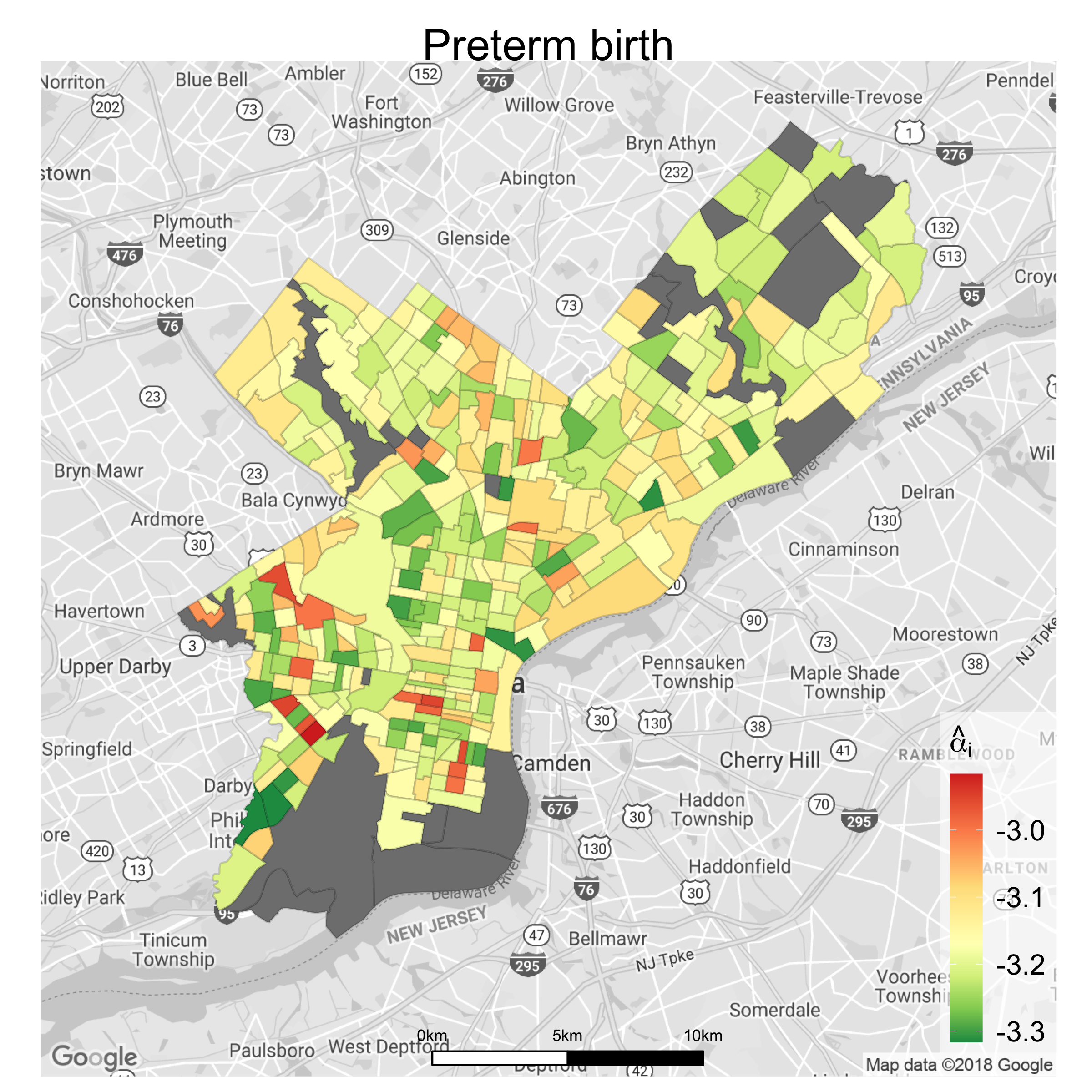
Figure 6: Maps of the posterior means of the neighborhood random effects $\alpha_{i}$ from the CAR model. Left panel: Results for stillbirth. Right panel: Results for preterm birth.

In Figure 6, we plot the posterior means $\widehat{\alpha}_{i}$’s of the neighborhood random effects for the 363 census tracts in our CAR model. Recall that the random effect $\alpha_{i}$ in (2) accounts for the variation in risk for neighborhood $i$ that cannot be explained by the fixed covariates $\bm{x}_{ij}$. Figure 3 is a bit easier to interpret than Figure 6, since Figure 3 depicts the predicted neighborhood risk probabilities of adverse pregnancy outcomes. However, we include Figure 6 here for the sake of completeness.

Appendix E MCMC diagnostics and additional computational details

E.1 MCMC diagnostics

In this section, we report the diagnostics for the MCMC algorithm described in Appendix B after we fit the CAR model to the Philadelphia dataset. Table 9 shows the effective sample size (ESS), posterior mean and Monte Carlo standard error (MCSE) for the regression coefficients (i.e. log-odds ratio) of the individual and neighborhood covariates. Results are reported in Table 9 for stillbirth and preterm birth.

Figure 7 shows the trace plots and autocorrelation plots of the MCMC samples for several of the regression coefficients under our CAR model. Figure 7 shows that the MCMC algorithm converged within 5500 iterations for the data that we analyzed in Section 4. Moreover, by thinning the chain every 10 iterations, our final MCMC samples were not overly correlated.

Table 9: Effective sample size (ESS), posterior mean regression coefficient ($\beta_{j}$), and Monte Carlo standard error (MCSE) for $\beta_{j}$ under the CAR model. These diagnostics are reported for both stillbirth and preterm birth.

	Stillbirth			Preterm birth
	ESS	$\beta_{j}$	MCSE	ESS	$\beta_{j}$	MCSE
Hispanic	168.2	-0.024	0.0239	662.0	0.449	0.0040
Black	68.3	0.450	0.0238	231.9	0.630	0.0060
Asian	190.3	0.131	0.0342	1011.8	-0.354	0.0047
multiple birth	943.7	2.356	0.0100	4241.4	1.408	0.0014
age	468.4	0.020	0.0035	2511.8	0.029	0.0006
proportion Asian	326.4	-0.016	0.0060	1609.8	-0.026	0.0011
proportion Hispanic	379.6	-0.053	0.0056	1839.4	-0.068	0.0011
proportion Black	293.8	-0.035	0.0111	1183.4	-0.061	0.0020
proportion women	386.6	0.038	0.0050	2064.8	-0.105	0.0008
poverty	450.3	-0.017	0.0059	2462.0	0.243	0.0010
public assistance	430.3	-0.003	0.0050	2249.7	-0.124	0.0008
labor force	399.5	-0.059	0.0062	2042.1	-0.050	0.0010
recent birth	461.4	0.017	0.0037	2230.2	0.038	0.0006
high school grad	432.0	0.109	0.0062	2212.4	0.068	0.0010
college grad	356.7	-0.074	0.0090	1780.7	-0.068	0.0015
occupied housing	377.2	-0.015	0.0054	1821.4	0.063	0.0009
housing violation	416.0	-0.033	0.0058	1869.5	-0.099	0.0011
violent crime	413.7	0.120	0.0097	1881.7	0.166	0.0017
nonviolent crime	375.0	-0.027	0.0064	1836.8	-0.086	0.0011

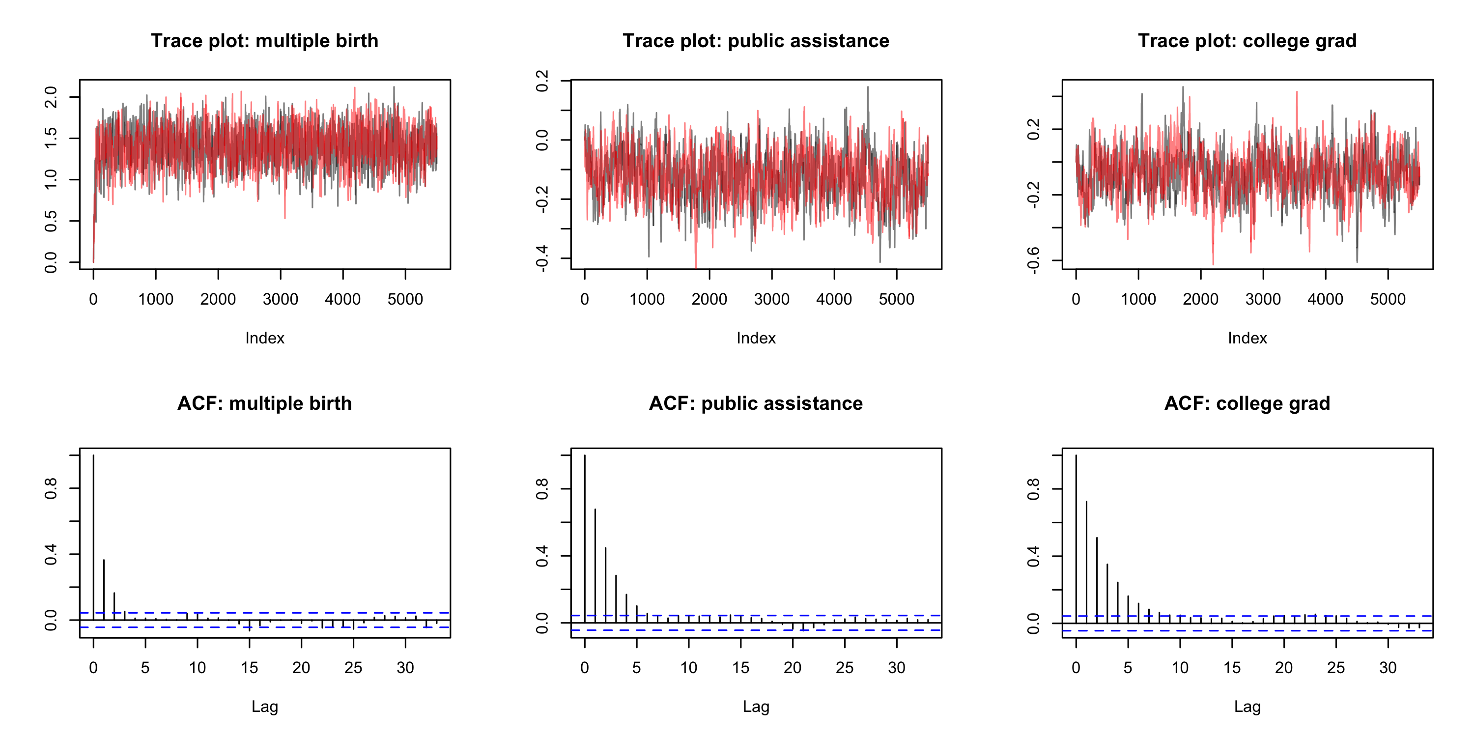
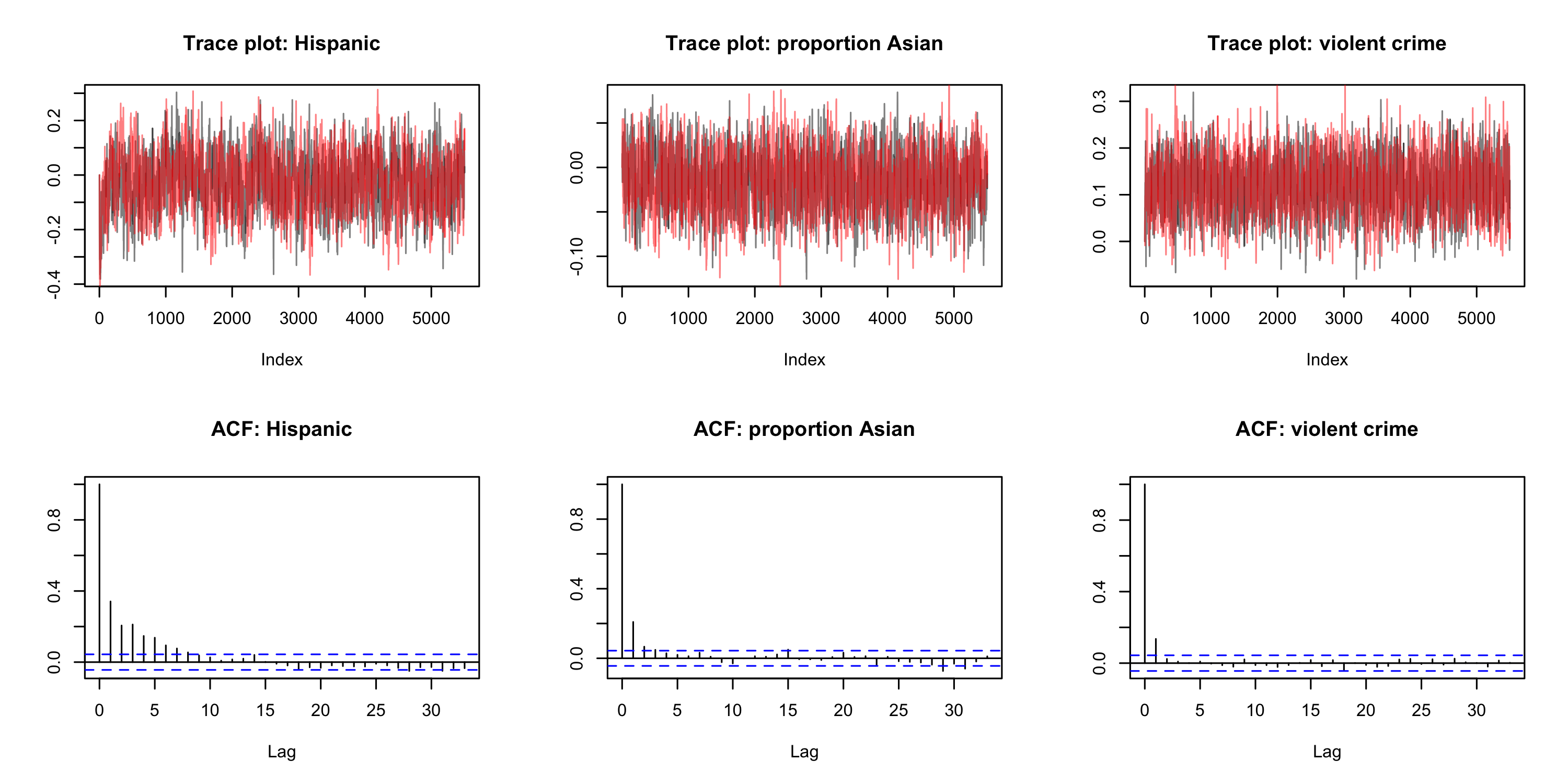
Figure 7: Trace plots of the two MCMC chains and autocorrelation plots of the thinned samples for several regression coefficients in our CAR model. In the top two rows, we plot the results for stillbirth, and in the bottom two rows, we plot the results for preterm birth.

E.2 R Packages used in the code implementation

All methods were implemented in the statistical environment R,[33] using the following R packages:

• BayesLogit [31]

• mvtnorm [11]

• xtable [8]

• sp [29]

• spdep [4]

• ggplot2 [41]

• ggmap [13]

• maptools [3]

• bde [34]

• LaplacesDemon [39]

References

- Balocchi and Jensen [2019] Balocchi, C. and Jensen, S. T. (2019). Spatial modeling of trends in crime over time in Philadelphia. The Annals of Applied Statistics, 13(4):2235–2259.
- Besag [1974] Besag, J. (1974). Spatial interaction and the statistical analysis of lattice systems. Journal of the Royal Statistical Society: Series B (Statistical Methodology), 36(2):192–225.
- Bivand and Lewin-Koh [2019] Bivand, R. and Lewin-Koh, N. (2019). maptools: Tools for Handling Spatial Objects. R package version 0.9-9.
- Bivand and Wong [2018] Bivand, R. and Wong, D. W. S. (2018). Comparing implementations of global and local indicators of spatial association. TEST, 27(3):716–748.
- Boland et al. [2021] Boland, M. R., Liu, J., Balocchi, C., Meeker, J., Bai, R., Mellis, I., Mowery, D. L., and Herman, D. (2021). Association of neighborhood-level factors and COVID-19 infection patterns in philadelphia using spatial regression. AMIA Joint Summits on Translational Science proceedings. AMIA Joint Summits on Translational Science,, 2021:545–554.
- Byrnes et al. [2015] Byrnes, J., Mahoney, R., Quaintance, C., Gould, J. B., Carmichael, S., Shaw, G. M., Showen, A., Phibbs, C., Stevenson, D. K., and Wise, P. H. (2015). Spatial and temporal patterns in preterm birth in the United States. Pediatric Research, (77):836–844.
- Canelón et al. [2021] Canelón, S. P., Burris, H. H., Levine, L. D., and Boland, M. R. (2021). Development and evaluation of MADDIE: Method to acquire delivery date information from electronic health records. International Journal of Medical Informatics, 145:104339.
- Dahl et al. [2019] Dahl, D. B., Scott, D., Roosen, C., Magnusson, A., and Swinton, J. (2019). xtable: Export Tables to LaTeX or HTML. R package version 1.8-4.
- Ferré et al. [2016] Ferré, C., Callaghan, W., Olson, C., Sharma, A., and Barfield, W. (2016). Effects of maternal age and age-specific preterm birth rates on overall preterm birth rates — United States, 2007 and 2014. MMWR Morbidity and Mortality Weekly Report, 65(43):1181–1184.
- Gelman et al. [2013] Gelman, A., Carlin, J. B., Stern, H. S., Dunson, D. B., Vehtari, A., and Rubin, D. B. (2013). Bayesian Data Analysis. CRC Press.
- Genz et al. [2020] Genz, A., Bretz, F., Miwa, T., Mi, X., Leisch, F., Scheipl, F., and Hothorn, T. (2020). mvtnorm: Multivariate Normal and t Distributions. R package version 1.1-0.
- Jardine et al. [2021] Jardine, J., Walker, K., Gurol-Urganci, I., Webster, K., Muller, P., Hawdon, J., Khalil, A., Harris, T., van der Meulen, J., Maternity, N., et al. (2021). Adverse pregnancy outcomes attributable to socioeconomic and ethnic inequalities in England: a national cohort study. The Lancet, 398(10314):1905–1912.
- Kahle and Wickham [2013] Kahle, D. and Wickham, H. (2013). ggmap: Spatial visualization with ggplot2. The R Journal, 5(1):144–161.
- Kramer et al. [2010] Kramer, M. R., Cooper, H. L., Drews-Botsch, C. D., Waller, L. A., and Hogue, C. R. (2010). Metropolitan isolation segregation and black–white disparities in very preterm birth: A test of mediating pathways and variance explained. Social Science and Medicine, 71(12):2108 – 2116.
- Kramer and Hogue [2008] Kramer, M. R. and Hogue, C. R. (2008). Place matters: Variation in the black/white very preterm birth rate across U.S. metropolitan areas, 2002–2004. Public Health Reports, 123(5):576–585.
- Kramer [2003] Kramer, M. S. (2003). The epidemiology of adverse pregnancy outcomes: An overview. The Journal of Nutrition, 133(5):1592S–1596S.
- Lee [2011] Lee, D. (2011). A comparison of conditional autoregressive models used in Bayesian disease mapping. Spatial and Spatio-temporal Epidemiology, 2(2):79–89.
- Leroux et al. [2000] Leroux, B. G., Lei, X., and Breslow, N. (2000). Estimation of disease rates in small areas: A new mixed model for spatial dependence. In Halloran, M. E. and Berry, D., editors, Statistical Models in Epidemiology, the Environment, and Clinical Trials, pages 179–191, New York, NY. Springer New York.
- Macdorman and Gregory [2015] Macdorman, M. F. and Gregory, E. C. W. (2015). Fetal and perinatal mortality: United States, 2013. National Vital Statistics Reports, 64(8):1–24.
- Makowski et al. [2019] Makowski, D., Ben-Shachar, M. S., Chen, S., and Lüdecke, D. (2019). Indices of effect existence and significance in the bayesian framework. Frontiers in Psychology, 10:2767.
- Martin et al. [2018] Martin, J., Hamilton, B., Osterman, M., Driscoll, A., Drake, P., and National Center for Health Statistics (U.S.) (2018). Births: Final data for 2017. National Vital Statistics Reports, 67(8).
- Masi et al. [2007] Masi, C. M., Hawkley, L. C., Piotrowski, Z. H., and Pickett, K. E. (2007). Neighborhood economic disadvantage, violent crime, group density, and pregnancy outcomes in a diverse, urban population. Social Science & Medicine, 65(12):2440–2457.
- Mattison et al. [2001] Mattison, D. R., Damus, K., Fiore, E., Petrini, J., and Alter, C. (2001). Preterm delivery: a public health perspective. Paediatric and Perinatal Epidemiology, 15(s2):7–16.
- McGowan et al. [2021] McGowan, V. J., Buckner, S., Mead, R., McGill, E., Ronzi, S., F., B., and Bambra, C. (2021). Examining the effectiveness of place-based interventions to improve public health and reduce health inequalities: an umbrella review. BMC Public Health, 21:1888.
- Meeker et al. [2021] Meeker, J. R., Canelón, S. P., Bai, R., Levine, L., and Boland, M. R. (2021). Individual-level and neighborhood-level risk factors for severe maternal morbidity. Obstetrics & Gynecology, 137(5):847–854.
- Moran [1950] Moran, P. A. P. (1950). Notes on continuous stochastic phenomena. Biometrika, 37:17–23.
- Muraskas and Parsi [2008] Muraskas, J. and Parsi, K. (2008). BART with targeted smoothing: An analysis of patient-specific stillbirth risk. AMA Journal of Ethics, 10(10):655–658.
- Neter et al. [2004] Neter, J., Kutner, M. H., Nachtsheim, C. J., and Wasserman, W. (2004). Applied Linear Statistical Models (4th ed.). McGraw-Hill Irwin.
- Pebesma and Bivand [2005] Pebesma, E. J. and Bivand, R. S. (2005). Classes and methods for spatial data in R. R News, 5(2):9–13.
- Polson et al. [2013a] Polson, N. G., Scott, J. G., and Windle, J. (2013a). Bayesian inference for logistic models using Pólya–Gamma latent variables. Journal of the American Statistical Association, 108(504):1339–1349.
- Polson et al. [2013b] Polson, N. G., Scott, J. G., and Windle, J. (2013b). Bayesian inference for logistic models using Pólya–Gamma latent variables. Journal of the American Statistical Association, 108(504):1339–1349.
- R Core Team [2020a] R Core Team (2020a). R: A Language and Environment for Statistical Computing. R Foundation for Statistical Computing, Vienna, Austria.
- R Core Team [2020b] R Core Team (2020b). R: A Language and Environment for Statistical Computing. R Foundation for Statistical Computing, Vienna, Austria.
- Santafe et al. [2022] Santafe, G., Calvo, B., Perez, A., and Lozano, J. A. (2022). bde: Bounded Density Estimation. R package version 1.0.1.1.
- Sharpe [2013] Sharpe, E. K. (2013). Targeted neighbourhood social policy: a critical analysis. Journal of Policy Research in Tourism, Leisure and Events, 5(2):158–171.
- South et al. [2012] South, A. P., Jones, D. E., Hall, E. S., Huo, S., Meinzen-Derr, J., Liu, L., and Greenberg, J. M. (2012). Spatial analysis of preterm birth demonstrates opportunities for targeted intervention. Maternal and Child Health Journal, 16:470–478.
- Spiegelhalter et al. [2002] Spiegelhalter, D. J., Best, N. G., Carlin, B. P., and Van Der Linde, A. (2002). Bayesian measures of model complexity and fit. Journal of the Royal Statistical Society: Series B (Statistical Methodology), 64(4):583–639.
- Starling et al. [2020] Starling, J. E., Murray, J. S., Carvalho, C. M., Bukowski, R. K., and Scott, J. G. (2020). BART with targeted smoothing: An analysis of patient-specific stillbirth risk. The Annals of Applied Statistics, 14(1):28–50.
- Statisticat & LLC [2021] Statisticat & LLC (2021). LaplacesDemon: Complete Environment for Bayesian Inference. R package version 16.1.6.
- Watanabe and Opper [2010] Watanabe, S. and Opper, M. (2010). Asymptotic equivalence of Bayes cross validation and widely applicable information criterion in singular learning theory. Journal of Machine Learning Research, 11(12):3571–3594.
- Wickham [2016] Wickham, H. (2016). ggplot2: Elegant Graphics for Data Analysis. Springer-Verlag New York.
- Xu et al. [2016] Xu, J., Murphy, S. L., Kochanek, K. D., and Bastian, B. A. (2016). Deaths: Final data for 2013. National Vital Statistics Reports, 10(10):1–119.
- Zahrieh et al. [2019a] Zahrieh, D., Oleson, J. J., and Romitti, P. A. (2019a). Bayesian point process modeling to quantify geographic regions of excess stillbirth risk. Geographical Analysis, 51(3):381–400.
- Zahrieh et al. [2019b] Zahrieh, D., Oleson, J. J., and Romitti, P. A. (2019b). Quantifying geographic regions of excess stillbirth risk in the presence of spatial and spatio-temporal heterogeneity. Spatial and Spatio-temporal Epidemiology, 29:97–109.