More Powerful Conditional Selective Inference for
Generalized Lasso by Parametric Programming

Abstract

Conditional selective inference (SI) has been studied intensively as a new statistical inference framework for data-driven hypotheses. The basic concept of conditional SI is to make the inference conditional on the selection event, which enables an exact and valid statistical inference to be conducted even when the hypothesis is selected based on the data. Conditional SI has mainly been studied in the context of model selection, such as vanilla lasso or generalized lasso. The main limitation of existing approaches is the low statistical power owing to over-conditioning, which is required for computational tractability. In this study, we propose a more powerful and general conditional SI method for a class of problems that can be converted into quadratic parametric programming, which includes generalized lasso. The key concept is to compute the continuum path of the optimal solution in the direction of the selected test statistic and to identify the subset of the data space that corresponds to the model selection event by following the solution path. The proposed parametric programming-based method not only avoids the aforementioned major drawback of over-conditioning, but also improves the performance and practicality of SI in various respects. We conducted several experiments to demonstrate the effectiveness and efficiency of our proposed method.

1 Introduction

As machine learning (ML) is applied to solve numerous practical problems, the quantification of the reliability of data-driven knowledge obtained by ML algorithms is becoming increasingly important. Among the various potential approaches for reliable ML, conditional selective inference (SI) has been recognized as a new promising method for assessing the statistical reliability of data-driven hypotheses that are selected by ML algorithms. The main concept of conditional SI is to make the inference for a data-driven hypothesis conditional on the selection event that the hypothesis is selected, which enables an exact and a valid inference to be conducted on the selected hypothesis. In the conditional SI framework, the statistical significance and reliability of data-driven selected hypotheses are quantified by the so-called selective $p$-values and selective confidence intervals, which have proper false positive rates and coverage guarantees, respectively.

Lee et al. (2016) first introduced conditional SI as a statistical inference tool for the features selected by lasso (Tibshirani, 1996). Subsequently, Hyun et al. (2018a) studied SI for inference on the selected model using generalized lasso (Tibshirani and Taylor, 2011). Their basic concept was to characterize the selection event using a polytope (a set of linear inequalities) in the sample space. In general, we refer to such methods as polytope-based SI approaches. The practical computational methods developed by these authors can be used when the selection event can be characterized by a single polytope.

However, the application scope of such polytope-based SI is limited because it can only be used when the characterization of all relevant selection events is represented by a polytope. Therefore, in most existing polytope-based SI studies, additional conditioning is required for the selection event to be characterized as a polytope. For example, in the case of lasso (Lee et al., 2016), the set of selected features as well as their signs require conditioning. Similarly, in the case of generalized lasso (Hyun et al., 2018a), additional conditioning on the signs as well as on the history (sequential order) whereby the selected elements enter the selected model is required. Such additional conditioning results in low statistical power, which is widely recognized as a major drawback of polytope-based SI studies (Fithian et al., 2014).

Contributions.

The contributions of this study are as follows:

• We go beyond the scope of polytope-based SI and propose a new SI approach based on parametric programming (PP). We name the proposed method PP-based SI. The basic concept of PP-based SI is to compute the continuum path of the optimal solutions in the direction of the selected test statistic using PP, which is subsequently used to identify the exact sampling distribution of the test statistic with the minimum amount of conditioning. Therefore, PP-based SI can fundamentally resolve the over-conditioning problem, which is a major concern in polytope-based SI, thereby achieving high statistical power.

• We derive the proposed PP-based SI for a generic class of conditional SI problems that can be represented as parametric quadratic programs (QPs). We demonstrate that the conditional SI formulations for many practical problems, including generalized lasso, elastic net, non-negative least squares, and Huber regression with the $\ell_{1}$ penalty, belong to this class, which means that the proposed PP-based SI can be used extensively.

• Furthermore, we discuss how the advantages of PP can be exploited for the effective performance of conditional SI in various data analysis tasks. As an example, using PP, we demonstrate that conditional SI can be conducted with minimal conditioning for regularization parameter selection by cross-validation (CV), the selection event of which is too complicated to be characterized as a single polytope, but can be fully characterized using PP.

• We conducted intensive experiments on both synthetic and real-world datasets, by means of which we presented evidence that our proposed method can successfully control the false positive rate, has higher statistical power than polytope-based SI, and provides superior results in practical applications.

A preliminary short version of this work was presented at the AI & Statistics (AISTATS2021) conference (Le Duy and Takeuchi, 2021). In the conference version, we only studied a specific case of vanilla lasso. In this study, we extended the basic concept of PP-based SI to a more general class of problems that can be formulated as parametric QPs, which includes vanilla lasso as a special case. Moreover, we extended the proposed method to various aspects and conducted intensive additional experiments to demonstrate the applicability of the generalized PP-based SI to a wider class of problems and settings.

Related works.

In traditional statistical inference, it is assumed that the hypothesis is fixed in advance. That is, the hypothesis on which we wish to conduct inference is determined prior to observing the dataset. Therefore, if traditional statistical inference methods are applied to data-driven hypotheses, the inferential results will no longer be valid. This problem has been discussed extensively in the context of testing the significance of the features selected by a feature selection method, such as lasso or stepwise feature selection. Several approaches have been proposed to address this problem (Benjamini and Yekutieli, 2005; Leeb and Pötscher, 2005, 2006; Benjamini et al., 2009; Pötscher and Schneider, 2010; Berk et al., 2013; Lockhart et al., 2014; Taylor et al., 2014).

In recent years, Lee et al. (2016) proposed a practical SI framework to perform exact (non-asymptotic) inference for a set of features selected by lasso. In their work, the authors revealed that the selection event can be characterized as a polytope by conditioning on a set of selected features and their signs. Furthermore, Hyun et al. (2018a) demonstrated that polytope-based SI is applicable to generalized lasso by performing additional conditioning on the signs as well as the history (sequential order) whereby the selected elements entered the selected model. Following the seminal work of (Lee et al., 2016), conditional inference-based SI has been actively studied and applied to various problems (Fithian et al., 2015; Choi et al., 2017; Tian and Taylor, 2018; Chen and Bien, 2019; Hyun et al., 2018b; Loftus and Taylor, 2014; Loftus, 2015; Panigrahi et al., 2016; Tibshirani et al., 2016; Yang et al., 2016; Suzumura et al., 2017; Tanizaki et al., 2020; Duy et al., 2020b, a; Sugiyama et al., 2020; Tsukurimichi et al., 2021).

It is desirable to conduct more powerful inference by conditioning on as little information as possible in conditional SI (Fithian et al., 2014). However, in polytope-based SI, an excessive amount of over-conditioning is required to represent the selection event using a single polytope. The authors of Lee et al. (2016) already mentioned the problem of over-conditioning and discussed the solution for removing the additional conditioning by enumerating all possible combinations of signs and taking the union over the resulting polyhedra. Unfortunately, such an enumeration for an exponentially increasing number of sign combinations is only feasible when the number of selected features is small. Loftus and Taylor (2014) extended polytope-based SI to cases in which the selection event is characterized by quadratic inequalities. Although we do not discuss quadratic inequality-based SI further, as it suffers from a similar over-conditioning issue, our proposed PP-based SI can also be applied to resolve the issue for this class of conditional SIs.

Our work was motivated by Liu et al. (2018), in which the authors proposed solutions to overcome the over-conditioning issue of polytope-based SI for vanilla lasso in certain special settings. In one of the settings, inference on the full model parameters in which conditional SI can be performed with minimal conditioning was studied, because a full model parameter is not dependent on other parameters. Moreover, our work was motivated by a discussion in the paper where the authors noted that multiple lasso fitting at a sequence of grid points may aid in alleviating over-conditioning. However, the authors did not suggest any practical computational methods to realize this concept. Furthermore, the conditional sampling distribution that is evaluated at a finite number of grid points only provides an approximation of the exact distribution, which means that the theoretical validity of the conditional SI is no longer guaranteed. Our proposed PP-based SI can be interpreted as a means of solving lasso at infinitely many grid points, which completely resolves these challenging problems. As another direction to resolve over-conditioning, Tian and Taylor (2018) and Terada and Shimodaira (2019) proposed methods using randomization. A drawback of these randomization-based approaches (including the simple data-splitting approach) is that further randomness is added in both the feature selection and inference stages.

PP has long been studied in the optimization field to solve a family of optimization problems that are parameterized by a scalar parameter (Ritter, 1984; Allgower and George, 1993; Gal, 1995; Best, 1996). Moreover, PP has been used in the context of the regularization path in ML (Osborne et al., 2000; Efron and Tibshirani, 2004; Hastie et al., 2004; Rosset and Zhu, 2007; Bach et al., 2006; Rosset and Zhu, 2007; Tsuda, 2007; Lee and Scott, 2007; Takeuchi et al., 2009; Takeuchi and Sugiyama, 2011; Karasuyama and Takeuchi, 2010; Hocking et al., 2011; Karasuyama et al., 2012; Ogawa et al., 2013; Takeuchi et al., 2013). The regularization path is a method of tracking the manner in which the optimal solution changes when the regularization parameter changes, which is useful for efficient model selection. Our main idea was to employ PP to track how the optimal solution and selected features change when the training dataset changes in the direction of the selected test statistic, which enables the exact sampling distribution of the test statistic that is conditional on the selection event to be identified. The power of the conditional SI introduced in the pioneering work of Lee et al. (2016) can be optimized using the proposed approach, which is applicable to conditional SI for a wide class of problems including generalized lasso.

2 Problem Statement

To formulate the problem, we consider a random response vector

$${\bm{Y}}=(Y_{1},...,Y_{n})^{\top}\sim\mathbb{N}({\bm{\mu}},\Sigma),$$ (1)

where $n$ is the number of instances, ${\bm{\mu}}$ is an unknown vector, and $\Sigma\in\mathbb{R}^{n\times n}$ is a covariance matrix that is known or estimable from independent data. The goal is statistical quantification of the significance of the data-driven hypotheses that are obtained by applying the generalized lasso estimator to the response vector.

Generalized lasso and its selection event.

We consider a linear regression model with $p$ features $\bm{x}_{1},\ldots,\bm{x}_{p}\in\mathbb{R}^{n}$ and denote the feature matrix as $X\in\mathbb{R}^{n\times p}$, in which the features are considered as non-random. We do not make any assumption about the relationship between the $\bm{\mu}$ and $p$ features $\bm{x}_{1},\ldots,\bm{x}_{p}\in\mathbb{R}^{n}$, but consider the case in which a linear model with generalized lasso regularization is employed to model the relationship between $X$ and a random response vector $\bm{Y}$. Given an observed response vector ${\bm{y}}^{\rm obs}\in\mathbb{R}^{n}$ that is sampled from model (1), the generalized lasso optimization problem is expressed as

$$\hat{{\bm{\beta}}}=\operatorname*{arg\,min}\limits_{{\bm{\beta}}\in\mathbb{R}^{p}}\frac{1}{2}\|{\bm{y}}^{\rm obs}-X{\bm{\beta}}\|^{2}_{2}+\lambda\|D{\bm{\beta}}\|_{1},$$ (2)

where $D\in\mathbb{R}^{m\times p}$ is a penalty matrix and $\lambda\geq 0$ is a regularization parameter. The matrix $D$ and its number of rows are predetermined by the user to produce the desired structures in the solution $\hat{\bm{\beta}}$ in (2). Examples of matrix $D$ are presented in Examples 1, 2, and 3.

As the optimization in (2) produces the sparsity of $D\hat{\bm{\beta}}$, we define a set of non-zero components (the active set) as follows:

$${\mathcal{M}}_{\rm obs}={\mathcal{A}}({\bm{y}}^{\rm obs})=\{j:(D\hat{\bm{\beta}})_{j}\neq 0\},\quad j\in[m],$$

where ${\mathcal{A}}:\bm{Y}\mapsto{\mathcal{M}}$ indicates the algorithm that maps a response vector $\bm{Y}$ to a set of non-zero components ${\mathcal{M}}$. Thereafter, we define the selection event in which the active set for a random response vector $\bm{Y}$ is the same as the observed response vector $\bm{y}^{\rm obs}$:

$$\left\{{\mathcal{A}}(\bm{Y})={\mathcal{A}}({\bm{y}}^{\rm obs})\right\}.$$ (3)

Statistical inference.

Let $\bm{\eta}^{\top}_{j}\bm{Y}$ be a linear contrast that indicates the test statistic that we wish to consider, where $\bm{\eta}_{j}$ is defined depending on the problem and the $j^{\rm th}$ selected component in the observed active set.

Example 1.

In the case of testing the features selected by vanilla lasso (Tibshirani, 1996), $D=I_{p}\in\mathbb{R}^{p\times p}$, which is the identity matrix. The test statistic $\bm{\eta}^{\top}_{j}\bm{Y}=\hat{\beta}_{j}$ represents the coefficient of the $j^{\rm th}$ selected feature (Lee et al., 2016), where $\bm{\eta}_{j}$ is defined as

$$\bm{\eta}_{j}=X_{{\mathcal{M}}_{\rm obs}}\left(X^{\top}_{{\mathcal{M}}_{\rm obs}}X_{{\mathcal{M}}_{\rm obs}}\right)^{-1}\bm{e}_{j},$$ (4)

in which $\bm{e}_{j}\in\mathbb{R}^{|{\mathcal{M}}_{\rm obs}|}$ is a basis vector with $1$ at the $j^{\rm th}$ position. This form of test statistic can also be applied to test the features that are selected by other regression methods, such as elastic net (Zou and Hastie, 2005), Huber regression (Huber, 1992), or non-negative least squares.

Example 2.

In the context of changepoint (CP) detection using fused lasso, the matrix $D\in\mathbb{R}^{(p-1)\times p}$ is expressed as

$$D=\begin{pmatrix}-1&1&0&\cdots&0&0\\ 0&-1&1&\cdots&0&0\\ &&&\cdots&&\\ 0&0&0&\cdots&-1&1\end{pmatrix}.$$

The test statistic $\bm{\eta}^{\top}_{j}\bm{Y}$ represents the difference in the sample mean between the left and right segments of the CP at the $j^{\rm th}$ position, which was also used in Hyun et al. (2018a). In this case, $\bm{\eta}_{j}$ is defined as

$$\bm{\eta}_{j}=\frac{1}{j-j_{\rm prev}}\mathbf{1}^{n}_{j_{\rm prev}+1:j}-\frac{1}{j_{\rm next}-j}\mathbf{1}^{n}_{j+1:j_{\rm next}},$$ (5)

where $j_{\rm prev}\in{\mathcal{M}}_{\rm obs}$ and $j_{\rm next}\in{\mathcal{M}}_{\rm obs}$ are the CP positions before and after the selected CP at position $j$, respectively, and $\mathbf{1}^{n}_{s:e}\in\mathbb{R}^{n}$ is a vector in which the elements from positions $s$ to $e$ are set to 1, and 0 otherwise.

Example 3.

In trend filtering, the aim is to test whether a change occurs in the trend at position $j\in{\mathcal{M}}_{\rm obs}$. We define $\bm{\eta}_{j}$ as follows:

$$\bm{\eta}_{j}=\bm{e}_{j-1}-2\bm{e}_{j}+\bm{e}_{j+1},$$

where $\bm{e}_{j}\in\mathbb{R}^{n}$. The test statistic $\bm{\eta}_{j}^{\top}\bm{Y}$ indicates that we wish to test whether the points at positions $j$, $j-1$, and $j+1$ lie on the same line statistically. In this case, the matrix $D\in\mathbb{R}^{(p-2)\times p}$ is expressed as

$$D=\begin{pmatrix}-1&2&-1&\cdots&0&0&0\\ 0&-1&2&\cdots&0&0&0\\ &&&\cdots&&&\\ 0&0&0&\cdots&-1&2&-1\end{pmatrix}.$$

For the inference, we consider the following null hypothesis and alternative hypothesis:

$${\rm H}_{0,j}:\bm{\eta}_{j}^{\top}\bm{\mu}=0\quad\text{vs.}\quad{\rm H}_{1,j}:\bm{\eta}_{j}^{\top}\bm{\mu}\neq 0.$$ (6)

Conditional SI.

Suppose that the hypotheses in (6) are fixed; that is, non-random. Thus, the naive (two-sided) $p$-value in the classical $z$-test is obtained by

$$P^{\rm naive}_{j}=\mathbb{P}_{{\rm H}_{0,j}}\left(|\bm{\eta}_{j}^{\top}\bm{Y}|\geq|\bm{\eta}_{j}^{\top}\bm{y}^{\rm obs}|\right).$$ (7)

However, as the hypotheses in (6) are not fixed in advance, the naive $p$-value is not valid in the sense that, if we reject ${\rm H}_{0,j}$ with a significance level $\alpha$ (e.g., $\alpha=0.05$), the false positive rate (type-I error) cannot be controlled at the level $\alpha$. This is because the hypotheses in (6) are selected by the data and selection bias exists.

It is necessary to remove the information that has been used for the initial hypothesis generation process to correct the selection bias. This can be achieved by considering the sampling distribution of the test statistic $\bm{\eta}^{\top}_{j}\bm{Y}$ that is conditional on the selection event; that is,

$$\bm{\eta}^{\top}_{j}\bm{Y}\mid\left\{{\mathcal{A}}(\bm{Y})={\mathcal{A}}({\bm{y}}^{\rm obs}),{\bm{q}}({\bm{Y}})={\bm{q}}({\bm{y}}^{\rm obs})\right\},$$ (8)

where ${\bm{q}}({\bm{Y}})=(I_{n}-{\bm{c}}{\bm{\eta}}^{\top}_{j}){\bm{Y}}$ with $\bm{c}=\Sigma{\bm{\eta}}_{j}({\bm{\eta}}^{\top}_{j}\Sigma{\bm{\eta}}_{j})^{-1}$ is the nuisance component that is independent of the test statistic $\bm{\eta}_{j}^{\top}\bm{Y}$. The second condition ${\bm{q}}({\bm{Y}})={\bm{q}}({\bm{y}}^{\rm obs})$ indicates that the nuisance component for a random vector $\bm{Y}$ is the same as that for $\bm{y}^{\rm obs}$ .

Once the selection event has been identified, the pivotal quantity can be computed:

$$F^{{\mathcal{Z}}}_{\bm{\eta}^{\top}_{j}\bm{\mu},{\bm{\eta}}^{\top}_{j}\Sigma{\bm{\eta}}_{j}}(\bm{\eta}^{\top}_{j}\bm{Y}).\mid\left\{{\mathcal{A}}(\bm{Y})={\mathcal{A}}({\bm{y}}^{\rm obs}),{\bm{q}}({\bm{Y}})={\bm{q}}({\bm{y}}^{\rm obs})\right\},$$ (9)

which is the c.d.f. of the truncated normal distribution with a mean $\bm{\eta}^{\top}_{j}\bm{\mu}$, variance ${\bm{\eta}}^{\top}_{j}\Sigma{\bm{\eta}}_{j}$, and truncation region ${\mathcal{Z}}$, which is calculated based on the selection event. Based on the pivotal quantity, the selective type-I error or selective $p$-value (Fithian et al., 2014) can be considered in the following form:

$$P^{\rm selective}_{j}=2\ \min\{\pi_{j},1-\pi_{j}\},$$ (10)

where $\pi_{j}=1-F^{{\mathcal{Z}}}_{0,{\bm{\eta}}^{\top}_{j}\Sigma{\bm{\eta}}_{j}}(\bm{\eta}^{\top}_{j}{\bm{Y}})$, which is valid in the sense that

$${\rm Prob}_{{\rm H}_{0,j}}\left(P^{\rm selective}_{j}<\alpha\right)=\alpha,\forall\alpha\in[0,1].$$

Furthermore, to obtain a confidence level of $1-\alpha$ for any $\alpha\in[0,1]$, by inverting the pivotal quantity in Equation (9), we can determine the smallest and largest values of $\bm{\eta}^{\top}_{j}\bm{\mu}$ such that the value of the pivotal quantity remains in the interval $\left[\frac{\alpha}{2},1-\frac{\alpha}{2}\right]$ (Lee et al., 2016).

Challenge in conditional data space characterization.

The main difficulty in the above conditional SI is that the characterization of the minimal conditional data space

$$\left\{{\mathcal{A}}(\bm{Y})={\mathcal{A}}({\bm{y}}^{\rm obs}),{\bm{q}}({\bm{Y}})={\bm{q}}({\bm{y}}^{\rm obs})\right\}$$

in Equation (8) is intractable. To overcome this issue, Hyun et al. (2018a) considered the inference to be conditional not only on the active set, but also on the signs and history (order) whereby the elements of $D\hat{\bm{\beta}}$ entered the active set. Unfortunately, such additional conditioning on the signs and history leads to low statistical power owing to over-conditioning .

In the following section, we introduce a method for identifying the minimum amount of conditioning $\left\{{\mathcal{A}}(\bm{Y})={\mathcal{A}}({\bm{y}}^{\rm obs}),{\bm{q}}({\bm{Y}})={\bm{q}}({\bm{y}}^{\rm obs})\right\}$ that results in higher statistical power. The main concept is to compute the path of the generalized lasso solutions in the direction of interest $\bm{\eta}_{j}$. By focusing on the line along $\bm{\eta}_{j}$, the majority of irrelevant regions that do not affect the truncated normal sampling distribution can be skipped because they do not intersect with this line. Thus, we can skip the majority of combinations of signs and history that never appear when applying generalized lasso to the data on the line.

3 Proposed Method

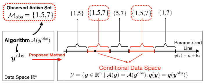
Figure 1: Schematic of proposed method. We obtain the observed active set ${\mathcal{M}}_{\rm obs}$ by applying generalized lasso to the observed data $\bm{y}^{\rm obs}$. The statistical inference for each selected element in the observed active set is conducted conditional on the subspace ${\mathcal{Y}}$, the data of which have the same active set as $\bm{y}^{\rm obs}$. We introduce a PP method for characterizing the conditional data space ${\mathcal{Y}}$ by searching the parameterized line.

We present the technical details of the proposed method in this section. A schematic of the method is provided in Figure 1. We first introduce a QP reformulation for the generalized lasso problem in §3.1. Thereafter, the characterization of the conditional data space is presented in §3.2. Subsequently, we propose a PP approach for identifying the conditional data space in §3.3. Finally, the detailed algorithm is presented in §3.4.

3.1 QP for Generalized Lasso

We demonstrate that the generalized lasso problem can be reformulated as a QP problem.

Lemma 1.

We denote $\bm{\xi}=D\bm{\beta}$, and the generalized lasso in (2) can be rewritten as

$$\left(\hat{\bm{\beta}},\hat{\bm{\xi}}\right)=\operatorname*{arg\,min}\limits_{\bm{\beta}\in\mathbb{R}^{p},\bm{\xi}\in\mathbb{R}^{m}}\frac{1}{2}||\bm{y}-X\bm{\beta}||_{2}^{2}+\lambda||\bm{\xi}||_{1}\quad\text{subject to}\quad\bm{\xi}=D\bm{\beta}.$$ (11)

By decomposing $\bm{\xi}=\bm{\xi}^{+}-\bm{\xi}^{-}$, $\bm{\xi}^{+},\bm{\xi}^{-}\geq\bm{0}$, the generalized lasso problem can be formulated as the following QP problem:

$$\begin{aligned} \left(\hat{\bm{\beta}},\hat{\bm{\xi}}^{+},\hat{\bm{\xi}}^{-}\right)=\operatorname*{arg\,min}\limits_{\bm{\beta},\bm{\xi}^{+},\bm{\xi}^{-}}&~{}\frac{1}{2}\begin{pmatrix}\bm{\beta}\\ \bm{\xi}^{+}\\ \bm{\xi}^{-}\end{pmatrix}^{\top}\begin{pmatrix}X^{\top}X&0&0\\ 0&0&0\\ 0&0&0\end{pmatrix}\begin{pmatrix}\bm{\beta}\\ \bm{\xi}^{+}\\ \bm{\xi}^{-}\end{pmatrix}+\left(\lambda\begin{pmatrix}\bm{0}_{p}\\ {\bm{1}}_{m}\\ {\bm{1}}_{m}\end{pmatrix}-\begin{pmatrix}X^{\top}\bm{y}\\ \bm{0}_{m}\\ \bm{0}_{m}\end{pmatrix}\right)^{\top}\begin{pmatrix}\bm{\beta}\\ \bm{\xi}^{+}\\ \bm{\xi}^{-}\end{pmatrix}\\ \textrm{s.t}~{}&\begin{pmatrix}0&I_{m}&-I_{m}\end{pmatrix}\begin{pmatrix}\bm{\beta}\\ \bm{\xi}^{+}\\ \bm{\xi}^{-}\end{pmatrix}=\begin{pmatrix}D&0&0\end{pmatrix}\begin{pmatrix}\bm{\beta}\\ \bm{\xi}^{+}\\ \bm{\xi}^{-}\end{pmatrix},~{}\bm{\xi}^{+}\geq 0,~{}\bm{\xi}^{-}\geq 0,\end{aligned}$$ (12)

where $\bm{1}_{m}\in\mathbb{R}^{m}$ and $\bm{0}_{m}\in\mathbb{R}^{m}$ are vectors in which all elements are set to 1 and 0, respectively, and $I_{m}\in\mathbb{R}^{m\times m}$ is an identity matrix.

Proof.

The optimization problem in (11) can be rewritten as follows:

$$\left(\hat{\bm{\beta}},\hat{\bm{\xi}}\right)=\operatorname*{arg\,min}\limits_{\bm{\beta},\bm{\xi}}\frac{1}{2}\bm{\beta}^{\top}X^{\top}X\bm{\beta}-(X^{\top}\bm{y})^{\top}\bm{\beta}+\lambda||\bm{\xi}||_{1}\quad\textrm{s.t}\quad\bm{\xi}=D\bm{\beta}.$$ (13)

We obtain (12) by decomposing $\bm{\xi}=\bm{\xi}^{+}-\bm{\xi}^{-}$ with $\bm{\xi}^{+},\bm{\xi}^{-}\geq\bm{0}$. In this case, the key point is that the component $||\bm{\xi}||_{1}$ in (13) can be written as $||\bm{\xi}||_{1}=\sum_{j\in[m]}(\xi^{+}_{j}+\xi^{-}_{j})$ because at least one of $\xi^{+}_{j}$ and $\xi^{-}_{j}$, $j\in[m]$, must be set to zero in the optimal solution. That is, $\hat{\xi}^{+}_{j}>0\Rightarrow\hat{\xi}^{-}_{j}=0$, and vice versa. The concept of decomposing $\bm{\xi}=\bm{\xi}^{+}-\bm{\xi}^{-}$ is often employed to reformulate the $\ell_{1}$-norm of $\bm{\xi}$. ∎

3.2 Conditional Data Space Characterization

We define the set of $\bm{y}\in\mathbb{R}^{n}$ that satisfies the conditions in Equation (8):

$${\mathcal{Y}}=\{{\bm{y}}\in\mathbb{R}^{n}\mid{\mathcal{A}}({\bm{y}})={\mathcal{A}}({\bm{y}}^{\rm obs}),{\bm{q}}(\bm{y})={\bm{q}}({\bm{y}}^{\rm obs})\}.$$ (14)

According to the second condition, the data in ${\mathcal{Y}}$ are restricted to a line (see Section 6 in Liu et al. (2018) and Fithian et al. (2014)). Therefore, the set ${\mathcal{Y}}$ can be rewritten using the scalar parameter $z\in\mathbb{R}$, as follows:

$${\mathcal{Y}}=\left\{{\bm{y}}(z)={\bm{a}}+{\bm{b}}z\mid z\in{\mathcal{Z}}\right\},$$ (15)

where ${\bm{a}}={\bm{q}}(\bm{y}^{\rm obs})$, ${\bm{b}}=\Sigma{\bm{\eta}}_{j}({\bm{\eta}}^{\top}_{j}\Sigma{\bm{\eta}}_{j})^{-1}$, and

$${\mathcal{Z}}=\left\{z\in\mathbb{R}\mid{\mathcal{A}}({\bm{y}}(z))={\mathcal{A}}({\bm{y}}^{\rm obs})\right\}.$$ (16)

Next, we consider a random variable $Z\in\mathbb{R}$ and its observation $z^{\rm obs}\in\mathbb{R}$, which satisfies ${\bm{Y}}={\bm{a}}+{\bm{b}}Z$ and ${\bm{y}}^{\rm obs}={\bm{a}}+{\bm{b}}z^{\rm obs}$. The conditional inference in (8) is rewritten as the problem of characterizing the sampling distribution of

$$Z\mid\left\{Z\in{\mathcal{Z}}\right\}.$$ (17)

As $Z\sim\mathbb{N}(0,{\bm{\eta}}^{\top}_{j}\Sigma{\bm{\eta}}_{j})$ under the null hypothesis, $Z\mid Z\in{\mathcal{Z}}$ follows a truncated normal distribution. Once the truncation region ${\mathcal{Z}}$ has been identified, the pivotal quantity in Equation (9) is equal to $F^{{\mathcal{Z}}}_{0,{\bm{\eta}}^{\top}_{j}\Sigma{\bm{\eta}}_{j}}(Z)$, and it can be obtained easily. Thus, the remaining task is the characterization of ${\mathcal{Z}}$.

Characterization of truncation region ${\mathcal{Z}}$.

We introduce the optimization problem (12) with the parameterized response vectors ${\bm{y}}(z)=\bm{a}+\bm{b}z$ ($\bm{a}$, $\bm{b}$ that are defined in (15)) for $z\in\mathbb{R}$ as follows:

$$\begin{aligned} \hat{\bm{r}}(z)=\operatorname*{arg\,min}_{\bm{r}}\quad&\frac{1}{2}\bm{r}^{\top}P\bm{r}+(\bm{q}^{0}+\bm{q}^{1}z)^{\top}\bm{r}\\ \textrm{s.t.}\quad&G\bm{r}\leq\bm{h}^{0}+\bm{h}^{1}z,\end{aligned}$$ (18)

where $\bm{r}=\left(\bm{\beta},\bm{\xi}^{+},\bm{\xi}^{-}\right)^{\top}\in\mathbb{R}^{p+2m}$, $\bm{q}^{0}=\left(-X^{\top}\bm{a},\lambda\bm{1}_{m},\lambda\bm{1}_{m}\right)^{\top}\in\mathbb{R}^{p+2m}$, $\bm{q}^{1}=\left(-X^{\top}\bm{b},\bm{0},\bm{0}\right)\in\mathbb{R}^{p+2m}$, $P\in\mathbb{R}^{(p+2m)\times(p+2m)}$ and $G\in\mathbb{R}^{4m\times(p+2m)}$, $\bm{h}^{0}=\bm{h}^{1}=\bm{0}_{4m}$,

$$P=\begin{pmatrix}X^{\top}X&0&0\\ 0&0&0\\ 0&0&0\end{pmatrix},\quad G=\begin{pmatrix}-D&D&0&0\\ I_{m}&-I_{m}&-I_{m}&0\\ -I_{m}&I_{m}&0&-I_{m}\\ \end{pmatrix}^{\top}.$$

Let $\hat{\bm{u}}(z)$ be the vector of optimal Lagrange multipliers and ${\rm row}(G)$ be the number of rows in matrix $G$. The KKT conditions of (18) are written as

$$P\hat{\bm{r}}(z)+\bm{q}^{0}+\bm{q}^{1}z+G^{\top}\hat{\bm{u}}(z) =0,$$ (19)

$$G\hat{\bm{r}}(z)-\bm{h}^{0}-\bm{h}^{1}z \leq 0,$$

$$\hat{u}_{i}(z)(G\hat{\bm{r}}(z)-\bm{h}^{0}-\bm{h}^{1}z)_{i} =0,\quad\forall i\in[{\rm row}(G)],$$

$$\hat{u}_{i}(z) \geq 0,\quad\forall i\in[{\rm row}(G)].$$

To construct the truncation region ${\mathcal{Z}}$ in Equation (16), we must 1) compute the entire path of $\hat{\bm{\xi}}(z)=\hat{\bm{\xi}}^{+}(z)-\hat{\bm{\xi}}^{-}(z)$ in (18), and 2) identify the set of intervals of $z$ on which ${\mathcal{A}}({\bm{y}}(z))={\mathcal{A}}({\bm{y}}^{\rm obs})$. However, it is difficult to compute $\hat{\bm{\xi}}^{+}(z)$ and $\hat{\bm{\xi}}^{-}(z)$ for infinitely many values of $z\in\mathbb{R}$. We demonstrate that the paths of $\hat{\bm{\xi}}^{+}(z)$ and $\hat{\bm{\xi}}^{-}(z)$ can be computed within finite operations by introducing parametric quadratic programming.

3.3 Piecewise Linear Homotopy

In this section, we demonstrate that $\hat{\bm{r}}(z)$ in (18) is a piecewise linear function of $z$, which also indicates that $\hat{\bm{\xi}}^{+}(z)$ and $\hat{\bm{\xi}}^{-}(z)$ are piecewise linear functions of $z$.

Lemma 2.

We denote ${\mathcal{I}}_{z}=\{i\in[{\rm row}(G)]:\hat{u}_{i}(z)>0\}$, ${\mathcal{I}}_{z}^{c}=[{\rm row}(G)]\setminus{\mathcal{I}}_{z}$, and $G_{{\mathcal{I}}_{z}}$ as the rows of matrix $G$ in a set ${\mathcal{I}}_{z}$. Consider two real values $z$ and $z^{\prime}$ ($z<z^{\prime}$). If ${\mathcal{I}}_{z}={\mathcal{I}}_{z^{\prime}}$, we obtain

$$\hat{\bm{r}}(z^{\prime})-\hat{\bm{r}}(z) =\bm{\psi}(z)\times(z^{\prime}-z),$$ (20)

$$\hat{\bm{u}}_{{\mathcal{I}}_{z}}(z^{\prime})-\hat{\bm{u}}_{{\mathcal{I}}_{z}}(z) =\bm{\gamma}(z)\times(z^{\prime}-z),$$ (21)

where $\bm{\psi}(z)\in\mathbb{R}^{{\rm row}(P)},\bm{\gamma}(z)\in\mathbb{R}^{|{\mathcal{I}}_{z}|}$, $\begin{bmatrix}\bm{\psi}(z)\\ \bm{\gamma}(z)\end{bmatrix}=\begin{bmatrix}P&G_{{\mathcal{I}}_{z}}^{\top}\\ G_{{\mathcal{I}}_{z}}&0\\ \end{bmatrix}^{-1}\begin{bmatrix}-\bm{q}^{1}\\ \bm{h}^{1}_{{\mathcal{I}}_{z}}\end{bmatrix}$.

Proof.

From the KKT conditions in (19), we obtain

$$P\hat{\bm{r}}(z)+\bm{q}^{0}+\bm{q}^{1}z+G^{\top}\hat{\bm{u}}(z) =0,$$ (22)

$$(G\hat{\bm{r}}(z)-\bm{h}^{0}-\bm{h}^{1}z)_{i} =0,\quad\forall i\in{\mathcal{I}}_{z},$$

$$(G\hat{\bm{r}}(z)-\bm{h}^{0}-\bm{h}^{1}z)_{i} \leq 0,\quad\forall i\in{\mathcal{I}}_{z}^{c}.$$

According to (22), we obtain the following linear system:

$$\begin{bmatrix}P&G_{{\mathcal{I}}_{z}}^{\top}\\ G_{{\mathcal{I}}_{z}}&0\end{bmatrix}\begin{bmatrix}\hat{\bm{r}}(z)\\ \hat{\bm{u}}_{{\mathcal{I}}_{z}}(z)\end{bmatrix}=\begin{bmatrix}-\bm{q}^{0}\\ \bm{h}^{0}_{{\mathcal{I}}_{z}}\end{bmatrix}+\begin{bmatrix}-\bm{q}^{1}\\ \bm{h}^{1}_{{\mathcal{I}}_{z}}\end{bmatrix}z$$

$$\Leftrightarrow~{} \begin{bmatrix}\hat{\bm{r}}(z)\\ \hat{\bm{u}}_{{\mathcal{I}}_{z}}(z)\end{bmatrix}=\begin{bmatrix}P&G_{{\mathcal{I}}_{z}}^{\top}\\ G_{{\mathcal{I}}_{z}}&0\end{bmatrix}^{-1}\begin{bmatrix}-\bm{q}^{0}\\ \bm{h}^{0}_{{\mathcal{I}}_{z}}\end{bmatrix}+\begin{bmatrix}P&G_{{\mathcal{I}}_{z}}^{\top}\\ G_{{\mathcal{I}}_{z}}&0\end{bmatrix}^{-1}\begin{bmatrix}-\bm{q}^{1}\\ \bm{h}^{1}_{{\mathcal{I}}_{z}}\end{bmatrix}z.$$ (23)

Similarly, for $z^{\prime}$, we obtain

$$\begin{bmatrix}\hat{\bm{r}}(z^{\prime})\\ \hat{\bm{u}}_{{\mathcal{I}}_{z^{\prime}}}(z^{\prime})\end{bmatrix}=\begin{bmatrix}P&G_{{\mathcal{I}}_{z^{\prime}}}^{\top}\\ G_{{\mathcal{I}}_{z^{\prime}}}&0\end{bmatrix}^{-1}\begin{bmatrix}-\bm{q}^{0}\\ \bm{h}^{0}_{{\mathcal{I}}_{z^{\prime}}}\end{bmatrix}+\begin{bmatrix}P&G_{{\mathcal{I}}_{z^{\prime}}}^{\top}\\ G_{{\mathcal{I}}_{z^{\prime}}}&0\end{bmatrix}^{-1}\begin{bmatrix}-\bm{q}^{1}\\ \bm{h}^{1}_{{\mathcal{I}}_{z^{\prime}}}\end{bmatrix}z^{\prime}.$$ (24)

By subtracting (23) from (24) and ${\mathcal{I}}_{z}={\mathcal{I}}_{z^{\prime}}$, we can express the following:

$$\begin{bmatrix}\hat{\bm{r}}(z^{\prime})\\ \hat{\bm{u}}_{{\mathcal{I}}_{z}}(z^{\prime})\end{bmatrix}-\begin{bmatrix}\hat{\bm{r}}(z)\\ \hat{\bm{u}}_{{\mathcal{I}}_{z}}(z)\end{bmatrix}=\begin{bmatrix}P&G_{{\mathcal{I}}_{z}}^{\top}\\ G_{{\mathcal{I}}_{z}}&0\end{bmatrix}^{-1}\begin{bmatrix}-\bm{q}^{1}\\ \bm{h}^{1}_{{\mathcal{I}}_{z}}\end{bmatrix}\times(z^{\prime}-z).$$ (25)

We denote $\begin{bmatrix}\bm{\psi}(z)\\ \bm{\gamma}(z)\end{bmatrix}=\begin{bmatrix}P&G_{{\mathcal{I}}_{z}}^{\top}\\ G_{{\mathcal{I}}_{z}}&0\end{bmatrix}^{-1}\begin{bmatrix}-\bm{q}^{1}\\ \bm{h}^{1}_{{\mathcal{I}}_{z}}\end{bmatrix}$ with $\bm{\psi}(z)\in\mathbb{R}^{{\rm row}(P)}$ and $\bm{\gamma}(z)\in\mathbb{R}^{|{\mathcal{I}}_{z}|}$, and we subsequently achieve the results in Lemma 2. ∎

For simplicity, we assume that the generalized lasso solution is unique for any $\bm{y}(z),z\in\mathbb{R}$. The uniqueness in the generalized lasso problem has been studied in Ali and Tibshirani (2019). In this case, it can be guaranteed that the matrix inverse in Equation (25) always exists. If this is not the case, we can use parametric quadratic programming for the degenerate cases in Best (1996).

Computation of breakpoint.

According to Lemma 2, the solution $\hat{\bm{r}}(z)$ is a linear function of $z$ until $z$ reaches a breakpoint, at which one component of $\hat{\bm{u}}(z)$ enters or leaves the set ${\mathcal{I}}_{z}$. At this point, we discuss the identification of the breakpoint.

Lemma 3.

Consider a real value $z$. Subsequently, ${\mathcal{I}}_{z}={\mathcal{I}}_{z^{\prime}}$ for any real value $z^{\prime}$ in the interval $[z,z+t_{z})$, where $z+t_{z}$ is the value of the breakpoint:

$$t_{z}=\min\{t_{z}^{1},t_{z}^{2}\}$$ , (26)

$$t_{z}^{1}=\min\limits_{j\in{\mathcal{I}}_{z}^{c}}\left(-\frac{(G_{{\mathcal{I}}^{c}_{z}}\hat{\bm{r}}(z)-\bm{h}^{0}_{{\mathcal{I}}_{z}^{c}}-\bm{h}^{1}_{{\mathcal{I}}_{z}^{c}}z)_{j}}{(G_{{\mathcal{I}}^{c}_{z}}\bm{\psi}(z)-\bm{h}^{1}_{{\mathcal{I}}_{z}^{c}})_{j}}\right)_{++}\quad \text{ and }\quad t_{z}^{2}=\min\limits_{j\in{\mathcal{I}}_{z}}\left(-\frac{\hat{u}_{j}(z)}{\gamma_{j}(z)}\right)_{++}.$$ (27)

In this case, for any $a\in\mathbb{R}$, $(a)_{++}=a$ if $a>0$, and $(a)_{++}=\infty$ otherwise.

Proof.

We first illustrate how to derive $t_{z}^{1}$. According to (20), we obtain

$$\hat{\bm{r}}(z^{\prime})=\hat{\bm{r}}(z)+\bm{\psi}(z)\times(z^{\prime}-z).$$

Thereafter, we need to guarantee

$$G_{{\mathcal{I}}^{c}_{z}}\hat{\bm{r}}(z^{\prime})-\bm{h}^{0}_{{\mathcal{I}}_{z}^{c}}-\bm{h}^{1}_{{\mathcal{I}}_{z}^{c}}z^{\prime} \leq 0$$

$$\Leftrightarrow~{}G_{{\mathcal{I}}^{c}_{z}}(\hat{\bm{r}}(z)+\bm{\psi}(z)\times(z^{\prime}-z))-\bm{h}^{0}_{{\mathcal{I}}_{z}^{c}}-\bm{h}^{1}_{{\mathcal{I}}_{z}^{c}}\times(z^{\prime}-z)-\bm{h}^{1}_{{\mathcal{I}}_{z}^{c}}z \leq 0$$

$$\Leftrightarrow~{}\left(G_{{\mathcal{I}}^{c}_{z}}\bm{\psi}(z)-\bm{h}^{1}_{{\mathcal{I}}_{z}^{c}}\right)\times(z^{\prime}-z) \leq-(G_{{\mathcal{I}}^{c}_{z}}\hat{\bm{r}}(z)-\bm{h}^{0}_{{\mathcal{I}}_{z}^{c}}-\bm{h}^{1}_{{\mathcal{I}}_{z}^{c}}z).$$ (28)

The right-hand side of (28) is positive because $G_{{\mathcal{I}}^{c}_{z}}\hat{\bm{r}}(z)-\bm{h}^{0}_{{\mathcal{I}}_{z}^{c}}-\bm{h}^{1}_{{\mathcal{I}}_{z}^{c}}z\leq 0$. Therefore, to satisfy Equation (28),

$$z^{\prime}-z\leq\min\limits_{j\in{\mathcal{I}}_{z}^{c}}\left(-\frac{(G_{{\mathcal{I}}^{c}_{z}}\hat{\bm{r}}(z)-\bm{h}^{0}_{{\mathcal{I}}_{z}^{c}}-\bm{h}^{1}_{{\mathcal{I}}_{z}^{c}}z)_{j}}{(G_{{\mathcal{I}}^{c}_{z}}\bm{\psi}(z)-\bm{h}^{1}_{{\mathcal{I}}_{z}^{c}})_{j}}\right)_{++}=t_{z}^{1}.$$

Next, we explain how to derive $t_{z}^{2}$. According to (21), we obtain

$$\hat{\bm{u}}_{{\mathcal{I}}_{z}}(z^{\prime})=\hat{\bm{u}}_{{\mathcal{I}}_{z}}(z)+\bm{\gamma}(z)\times(z^{\prime}-z).$$

We need to guarantee

$$\hat{\bm{u}}_{{\mathcal{I}}_{z}}(z^{\prime})>0\Leftrightarrow\hat{\bm{u}}_{{\mathcal{I}}_{z}}(z)+\bm{\gamma}(z)\times(z^{\prime}-z)>0.$$ (29)

Therefore, to satisfy Equation (29),

$$z^{\prime}-z<\min\limits_{j\in{\mathcal{I}}_{z}}\left(-\frac{\hat{u}_{j}(z)}{\gamma_{j}(z)}\right)_{++}=t_{z}^{2}.$$

Finally, using $t_{z}=\min\{t_{z}^{1},t_{z}^{2}\}$, we obtain the interval in which ${\mathcal{I}}_{z^{\prime}}={\mathcal{I}}_{z}$ for any $z^{\prime}\in[z,z+t_{z})$. ∎

3.4 Algorithm

0:  $X,{\bm{y}}^{\rm obs},\lambda,D,[z_{\rm min},z_{\rm max}]$

1:  Obtain observed active set ${\mathcal{M}}_{\rm obs}={\mathcal{A}}(\bm{y}^{\rm obs})$ for data $(X,{\bm{y}}^{\rm obs})$

2:  for each selected $j\in{\mathcal{M}}_{\rm obs}$ do

3:     Compute $\bm{\eta}_{j}$, and subsequently calculate $\bm{a}$ and $\bm{b}$ based on $\bm{\eta}_{j}$ and $\bm{y}^{\rm obs}$ $\leftarrow$ Equation (15)

4:     ${\mathcal{A}}(\bm{y}(z))\leftarrow{\tt compute\_solution\_path}$ ($X$, $\lambda$, $D$, $\bm{a}$, $\bm{b}$, $[z_{\rm min},z_{\rm max}]$)

5:     Truncation region ${\mathcal{Z}}\leftarrow\{z:{\mathcal{A}}(\bm{y}(z))={\mathcal{M}}_{\rm obs}\}$

6:     $P^{\rm selective}_{j}\leftarrow$ Equation (10) (and$/$or selective confidence interval)

7:  end for

7:  $\{P^{\rm selective}_{j}\}_{j\in{\mathcal{M}}_{\rm obs}}$ (and$/$or selective confidence intervals)

Algorithm 1 parametric_SI

0:  $X,\lambda,D,\bm{a},\bm{b},[z_{\rm min},z_{\rm max}]$

1:  Initialization: $k=1$, $z_{k}=z_{\rm min}$, ${\mathcal{T}}={z_{k}}$

2:  while $z_{k}<z_{\rm max}$ do

3:     $t_{z_{k}},{\mathcal{M}}_{z_{k}}\leftarrow{\tt compute\_step\_size}(X,z_{k},\bm{a},\bm{b},\lambda,D)$

4:     $z_{k+1}=z_{k}+t_{z_{k}}$, ${\mathcal{T}}={\mathcal{T}}\cup\{z_{k+1}\}$ ($z_{k+1}$ is the value of the next breakpoint)

5:     $k=k+1$

6:  end while

6:  $\{{\mathcal{M}}_{z_{k}}\}_{k\in[|{\mathcal{T}}|-1]}$

Algorithm 2 compute_solution_path

0:  $X,z,\bm{a},\bm{b},\lambda,D$

1:  $\bm{y}(z)=\bm{a}+\bm{b}z$

2:  Compute $\hat{\bm{r}}(z)$ for data $(X,\bm{y}(z))$ and calculate $\hat{\bm{\xi}}(z)=\hat{\bm{\xi}}^{+}(z)-\hat{\bm{\xi}}^{-}(z)$ based on $\hat{\bm{r}}(z)$

3:  Obtain ${\mathcal{M}}_{z}={\mathcal{A}}(\bm{y}(z))=\{j:\hat{\xi}_{j}(z)\neq 0\}$

4:  Compute $t_{z}$ $\leftarrow$ Lemma 3

4:  $t_{z},{\mathcal{M}}_{z}$

Algorithm 3 compute_step_size

In this section, we present the detailed algorithm of the proposed PP-based SI method. In Algorithm 1, to obtain the active set, we simply apply generalized lasso to the data $(X,\bm{y}^{\rm obs})$, and we obtain ${\mathcal{M}}_{\rm obs}$. Thereafter, we conduct SI for each observed active set. For every $j\in{\mathcal{M}}_{\rm obs},$ we first obtain the direction of interest $\bm{\eta}_{j}$. The main task is to compute the solution path of $\hat{\bm{r}}(z)$ in Equation (18) for the parameterized response vector $\bm{y}(z)$, where the parameterized solution $\hat{\bm{r}}(z)$ varies for different $j\in{\mathcal{M}}_{\rm obs}$ because the direction of interest $\bm{\eta}_{j}$ is dependent on $j$. This task can be achieved by Algorithm 2. Finally, after obtaining the path, we can easily determine the truncation region ${\mathcal{Z}}$, which is used to compute the selective $p$-value or selective confidence interval.

In Algorithm 2, a sequence of breakpoints is computed individually. The algorithm is initialized at $z_{k}=z_{\rm min},k=1$. At each $z_{k}$, the task is to determine the next breakpoint $z_{k+1}$. This task can be performed by computing the step size in Algorithm 3. This step is repeated until $z_{k}>z_{\rm max}$. By identifying all of the breakpoints $\{z_{t}\}_{t\in[|{\mathcal{T}}|]}$, the entire path of ${\mathcal{M}}_{z}$ for $z\in\mathbb{R}$ is expressed as

$${\mathcal{M}}_{z}={\mathcal{A}}(\bm{y}(z))=\left\{\begin{array}[]{ll}{\mathcal{A}}(\bm{y}(z_{1}))&\text{ if }z\in[z_{1},z_{2}],\\ {\mathcal{A}}(\bm{y}(z_{2}))&\text{ if }z\in[z_{2},z_{3}],\\ ~{}~{}~{}~{}~{}\vdots&\\ {\mathcal{A}}(\bm{y}(z_{|{\mathcal{T}}|-1}))&\text{ if }z\in[z_{|{\mathcal{T}}|-1},z_{|{\mathcal{T}}|}].\end{array}\right.$$

Selection of $[z_{\rm min},z_{\rm max}]$.

Under normality, very positive and negative values of $z$ do not affect the inference. Therefore, it is reasonable to consider a range of values, such as $[-20\sigma,20\sigma]$ (Liu et al., 2018) or $\left[-|\bm{\eta}_{j}^{\top}\bm{y}^{\rm obs}|-20\sigma,|\bm{\eta}_{j}^{\top}\bm{y}^{\rm obs}|+20\sigma\right]$ (Sugiyama et al., 2020), where $\sigma$ is the standard deviation of the sampling distribution of the test statistic.

In Line 2 of Algorithm 3, $\hat{\bm{r}}(z)$ can be computed based on the KKT conditions. However, it is well known that numerical issues will arise. Therefore, in our experiments, we modify the algorithm slightly to overcome these numerical problems. In particular, we first replace Line 1 in Algorithm 3 with $\bm{y}(z)=\bm{a}+\bm{b}(z+\Delta z)$, where $\Delta z$ is a small value such that $z_{k}+\Delta z<z_{k+1}$ for all $k\in[|{\mathcal{T}}|-1]$. Subsequently, at Line 2 of Algorithm 3, we simply obtain $\hat{\bm{r}}(z)$ by applying the QP solver to $\bm{y}(z)$. We can confirm whether $\Delta z$ is sufficiently small by verifying whether exactly one component in the vector of the optimal Lagrange multipliers $\hat{\bm{u}}(z)$ has already entered or left the set ${\mathcal{I}}_{z}$. This condition is satisfied in all of the experiments by simply setting $\Delta z=0.0001$.

The complexity of Algorithm 1 is dependent on the number of breakpoints. In the literature on PP, the worst-case complexity increases exponentially with the problem size (Ritter, 1984; Allgower and George, 1993; Gal, 1995; Best, 1996; Mairal and Yu, 2012). However, in practice, it has been reported that the number of breakpoints is approximately linear with the problem size and it does not actually increase as much as in the theoretical worst case. This has also been noted in regularization path studies (Osborne et al., 2000; Efron and Tibshirani, 2004; Hastie et al., 2004; Mairal and Yu, 2012). In fact, in all of the experiments in §6, the number of breakpoints is within a reasonable size and the computational cost is not a major problem of the proposed method.

4 Generality of Proposed Method

Although we only focused on generalized lasso in §3, the parametric QP formulation in (18) is more general and the forms of matrices $P$ and $G$ as well as vectors $\bm{q}^{0},\bm{q}^{1},\bm{h}^{0}$, and $\bm{h}^{1}$ can be changed depending on the problem. That is, the method proposed method in §3 is flexible and can be applied to any problem that can be converted into a parametric QP in the form of (18). In this section, we demonstrate the extensions of the proposed method for testing the statistical significance of the features that are selected by various feature selection algorithms.

When applying a feature selection algorithm ${\mathcal{A}}$ to the observed response vector $\bm{y}^{\rm obs}$, the observed active set can be defined as follows:

$${\mathcal{M}}_{\rm obs}={\mathcal{A}}(\bm{y}^{\rm obs})=\{j:\hat{\beta}_{j}\neq 0\}.$$

In this setting, $D=I_{p}$. To test the selected features in ${\mathcal{M}}_{\rm obs}$, the conditional inference is the same as that defined in (8) and the characterization of the truncation region ${\mathcal{Z}}$ is the same as (16). To identify ${\mathcal{Z}}$, the remaining task is to compute the solution path $\hat{\bm{\beta}}(z)$ for $z\in\mathbb{R}$ and to identify the intervals of $z$ in which we obtain the same active set as $\bm{y}^{\rm obs}$. In the following sections, we present the parametric QP formulations for vanilla lasso, elastic net, non-negative least squares, and Huber regression. As all of these regression problems can be converted into the form of (18), the path of $\hat{\bm{\beta}}(z)$ can be computed within finite operations by using PP, as demonstrated in §3.3.

Parametric QP for vanilla lasso.

Vanilla lasso with a parameterized response vector $\bm{y}(z)$ for $z\in\mathbb{R}$ is defined as

$$\hat{\bm{\beta}}_{\rm lasso}(z) =\operatorname*{arg\,min}\limits_{\bm{\beta}\in\mathbb{R}^{p}}\frac{1}{2}||\bm{y}(z)-X\bm{\beta}||_{2}^{2}+\lambda||\bm{\beta}||_{1}.$$ (30)

Lemma 4.

By decomposing $\bm{\beta}=\bm{\beta}^{+}-\bm{\beta}^{-}$, $\bm{\beta}^{+},\bm{\beta}^{-}\geq\bm{0}_{p}$, the lasso problem in (30) can be solved by the following parametric QP:

$$\left(\hat{\bm{\beta}}^{+}_{\rm lasso}(z),\hat{\bm{\beta}}^{-}_{\rm lasso}(z)\right)=\operatorname*{arg\,min}\limits_{\bm{\beta}^{+},\bm{\beta}^{-}\in\mathbb{R}^{p}} \quad\frac{1}{2}\begin{pmatrix}\bm{\beta}^{+}\\ \bm{\beta}^{-}\end{pmatrix}^{\top}\begin{pmatrix}X^{\top}X&-X^{\top}X\\ -X^{\top}X&X^{\top}X\end{pmatrix}\begin{pmatrix}\bm{\beta}^{+}\\ \bm{\beta}^{-}\end{pmatrix}$$

$$\quad+\left(\lambda\bm{1}_{2p}-\begin{pmatrix}X^{\top}\bm{y}(z)\\ -X^{\top}\bm{y}(z)\end{pmatrix}\right)^{\top}\begin{pmatrix}\bm{\beta}^{+}\\ \bm{\beta}^{-}\end{pmatrix}$$

s.t. $$\quad\bm{\beta}^{+}\geq\bm{0}_{p},\bm{\beta}^{-}\geq\bm{0}_{p}.$$

Proof.

According to (30), we obtain

$$\hat{\bm{\beta}}_{\rm lasso}(z) =\operatorname*{arg\,min}\limits_{\bm{\beta}\in\mathbb{R}^{p}}\frac{1}{2}||\bm{y}(z)-X\bm{\beta}||_{2}^{2}+\lambda||\bm{\beta}||_{1}$$

$$=\operatorname*{arg\,min}\limits_{\bm{\beta}\in\mathbb{R}^{p}}\frac{1}{2}\left(\bm{y}(z)^{\top}\bm{y}(z)-\bm{\beta}^{\top}X^{\top}\bm{y}(z)-\bm{y}(z)^{\top}X\bm{\beta}+\bm{\beta}^{\top}X^{\top}X\bm{\beta}\right)+\lambda||\bm{\beta}||_{1}.$$ (31)

Similar to the proof of Lemma 1, as the component $\frac{1}{2}\bm{y}(z)^{\top}\bm{y}(z)$ does not affect the optimal solution $\hat{\bm{\beta}}_{\rm lasso}(z)$, we can rewrite (31) as

$$\hat{\bm{\beta}}_{\rm lasso}(z)=\operatorname*{arg\,min}\limits_{\bm{\beta}\in\mathbb{R}^{p}}\frac{1}{2}\bm{\beta}^{\top}X^{\top}X\bm{\beta}-(X^{\top}\bm{y}(z))^{\top}\bm{\beta}+\lambda||\bm{\beta}||_{1}.$$ (32)

Finally, by decomposing $\bm{\beta}=\bm{\beta}^{+}-\bm{\beta}^{-}$, $\bm{\beta}^{+},\bm{\beta}^{-}\geq\bm{0}_{p}$ and $||\bm{\beta}||_{1}=\sum_{j\in[p]}(\beta^{+}_{j}+\beta^{-}_{j})$, we obtain the result in Lemma 4. ∎

In our preliminary conference paper (Le Duy and Takeuchi, 2021), we initially presented the idea of introducing PP for vanilla lasso in a slightly different (but essentially the same) manner.

Parametric QP for elastic net.

The elastic net with a parameterized response vector $\bm{y}(z)$ for $z\in\mathbb{R}$ is defined as

$$\hat{\bm{\beta}}_{\rm elastic}(z)=\operatorname*{arg\,min}\limits_{\bm{\beta}\in\mathbb{R}^{p}}\frac{1}{2n}||\bm{y}(z)-X\bm{\beta}||_{2}^{2}+\lambda||\bm{\beta}||_{1}+\frac{1}{2}\zeta||\bm{\beta}||_{2}^{2}.$$ (33)

Lemma 5.

By decomposing $\bm{\beta}=\bm{\beta}^{+}-\bm{\beta}^{-}$, $\bm{\beta}^{+},\bm{\beta}^{-}\geq\bm{0}_{p}$, the elastic net problem in (33) can be solved using the following parametric QP:

$$\left(\hat{\bm{\beta}}^{+}_{\rm elastic}(z),\hat{\bm{\beta}}^{-}_{\rm elastic}(z)\right)=\operatorname*{arg\,min}\limits_{\bm{\beta}^{+},\bm{\beta}^{-}\in\mathbb{R}^{p}} \quad\frac{1}{2n}\begin{pmatrix}\bm{\beta}^{+}\\ \bm{\beta}^{-}\end{pmatrix}^{\top}\begin{pmatrix}X^{\top}X&-X^{\top}X\\ -X^{\top}X&X^{\top}X\end{pmatrix}\begin{pmatrix}\bm{\beta}^{+}\\ \bm{\beta}^{-}\end{pmatrix}$$

$$\quad+\zeta\cdot\frac{1}{2}\begin{pmatrix}\bm{\beta}^{+}\\ \bm{\beta}^{-}\end{pmatrix}^{\top}\begin{pmatrix}I_{p}&-I_{p}\\ -I_{p}&I_{p}\end{pmatrix}\begin{pmatrix}\bm{\beta}^{+}\\ \bm{\beta}^{-}\end{pmatrix}\$$

$$\quad+\left(\lambda\bm{1}_{2p}-\frac{1}{n}\begin{pmatrix}X^{\top}\bm{y}(z)\\ -X^{\top}\bm{y}(z)\end{pmatrix}\right)^{\top}\begin{pmatrix}\bm{\beta}^{+}\\ \bm{\beta}^{-}\end{pmatrix}$$

s.t. $$\quad\bm{\beta}^{+}\geq\bm{0}_{p},\bm{\beta}^{-}\geq\bm{0}_{p}.$$

Proof.

The proof of Lemma 5 is similar to the proof of Lemma 4. ∎

Parametric QP for non-negative least squares.

The non-negative least squares problem with a parametrized response vector $\bm{y}(z)$ for $z\in\mathbb{R}$ is defined as

$$\hat{\bm{\beta}}_{\rm non-negative}(z)=\operatorname*{arg\,min}\limits_{\bm{\beta}\in\mathbb{R}^{p}}\frac{1}{2}||\bm{y}(z)-X\bm{\beta}||_{2}^{2}\quad\textrm{s.t}\quad\bm{\beta}\geq 0.$$

The above problem can be formulated as the following parametric QP:

$$\hat{\bm{\beta}}_{\rm non-negative}(z)=\operatorname*{arg\,min}\limits_{\bm{\beta}\in\mathbb{R}^{p}}\frac{1}{2}\bm{\beta}^{\top}X^{\top}X\bm{\beta}-\left(X^{\top}\bm{y}(z)\right)^{\top}\bm{\beta}\quad\textrm{s.t}\quad\bm{\beta}\geq 0.$$

Parametric QP for Huber regression with $\ell_{1}$ penalty.

The Huber regression with the $\ell_{1}$ penalty for a parameterized response vector $\bm{y}(z)$ is formulated as

$$\hat{\bm{\beta}}_{\rm huber}(z)=\operatorname*{arg\,min}_{\bm{\beta}\in\mathbb{R}^{p}}\sum_{i=1}^{n}L_{\delta}(y_{i}(z)-\bm{x}_{i}^{\top}\bm{\beta})+\lambda||\bm{\beta}||_{1},$$ (34)

with

$$L_{\delta}(e)=\left\{\begin{array}[]{ll}\frac{1}{2}e^{2}&\text{ if }|e|\leq\delta,\\ \delta(|e|-\frac{1}{2}\delta)&\text{ otherwise},\end{array}\right.$$

where $\delta>0$ is also a predetermined tuning parameter. Let $\bm{e}=\bm{y}(z)-X\bm{\beta}$, $\bm{\phi}\in\mathbb{R}^{n}$, and $\bm{\nu}\in\mathbb{R}^{n}$ be the vectors in which the $i^{\rm th}$ element $\phi_{i}$ and $\nu_{i}$ are respectively defined as

$$\phi_{i}=\min\{|e_{i}|,\delta\},\quad\nu_{i}=\max\{|e_{i}|-\delta,0\},$$

where $e_{i}$ is the $i^{\rm th}$ element of $\bm{e}$. Obviously, $|e_{i}|=\phi_{i}+\nu_{i}$. Subsequently, by decomposing $\bm{\beta}=\bm{\beta}^{+}-\bm{\beta}^{-}$, $\bm{\beta}^{+},\bm{\beta}^{-}\geq\bm{0}_{p}$, the problem in (34) can be solved by the following parametric QP:

$$\left(\hat{\bm{\phi}}(z),\hat{\bm{\nu}}(z),\hat{\bm{\beta}}^{+}_{\rm huber}(z),\hat{\bm{\beta}}^{-}_{\rm huber}(z)\right)=\operatorname*{arg\,min}\limits_{\bm{\phi},\bm{\nu},\bm{\beta}^{+},\bm{\beta}^{-}} \frac{1}{2}\bm{\phi}^{\top}\bm{\phi}+\delta\cdot\bm{1}_{n}^{\top}\bm{\nu}+\sum\limits_{j}\left(\beta_{j}^{+}+\beta_{j}^{-}\right)$$

s.t $$-\bm{\phi}-\bm{\nu}\leq\bm{y}(z)-X\left(\bm{\beta}^{+}-\bm{\beta}^{-}\right)\leq\bm{\phi}+\bm{\nu},$$

$$\bm{0}_{n}\leq\bm{u}\leq\delta\cdot\bm{1}_{n},~{}\bm{v}\geq\bm{0}_{n},$$

$$\bm{\beta}^{+}\geq\bm{0}_{p},~{}\bm{\beta}^{-}\geq\bm{0}_{p}.$$

The lasso-like formulation of the Huber regression has been discussed in She and Owen (2011). Conditional SI for outliers was studied in Chen and Bien (2019), and we recently investigated its PP version in Tsukurimichi et al. (2021).

5 Characterization of CV-Based Tuning Parameter Selection Event

Various ML tasks involve careful tuning of a regularization parameter $\lambda$ that controls the balance between an empirical loss term and a regularization term; for example, this is commonly achieved by CV. However, the majority of the current SI studies have assumed a pre-specified $\lambda$ and have ignored the fact that $\lambda$ is selected based on the data, because it is difficult to characterize the CV selection event. Loftus (2015) and Markovic et al. (2017) proposed solutions to incorporate CV events. However, the former work required additional conditioning on all intermediate models, which led to a loss of power, whereas the latter considered a randomization version of CV instead of vanilla CV.

In this section, we introduce a new means of characterizing the minimal selection event in which $\lambda$ is selected based on the data; for example, via CV . For notational simplicity, we consider the case in which the data are divided into training and validation sets, and the latter is used for selecting $\lambda$. The following discussion can easily be extended to CV scenarios. We rewrite the observed data as follows:

$$\{X,\bm{y}^{\rm obs}\}=\left\{(X_{\rm train}\ X_{\rm val})^{\top}\in\mathbb{R}^{n\times p},(\bm{y}^{\rm obs}_{\rm train}\ \bm{y}^{\rm obs}_{\rm val})^{\top}\in\mathbb{R}^{n}\right\}.$$

Given a set of regularization parameter candidates $\Lambda$, the process of selecting $\lambda$ is as follows:

1. For each $\lambda\in\Lambda$, we first obtain $\hat{\bm{\beta}}_{\lambda}$ using the training data

   $$\hat{\bm{\beta}}_{\lambda}\in\operatorname*{arg\,min}\limits_{\bm{\beta}}\frac{1}{2}\|\bm{y}_{\rm train}^{\rm obs}-X_{\rm train}\bm{\beta}\|^{2}_{2}+\lambda\|D\bm{\beta}\|_{1}.$$

   Thereafter, the validation error is defined as

   $$E_{\lambda}=\frac{1}{2}\|\bm{y}_{\rm val}^{\rm obs}-X_{\rm val}\bm{\hat{}}{\bm{\beta}}_{\lambda}\|^{2}_{2}.$$

2. We select $\lambda^{\rm obs}=\lambda\in\Lambda$, which has the corresponding smallest validation error $E_{\lambda}$.

The selection event of the above validation process is defined as

$$\{{\mathcal{V}}(\bm{Y})={\mathcal{V}}(\bm{y}^{\rm obs})\},$$ (35)

where ${\mathcal{V}}(\bm{y}^{\rm obs})=\lambda^{\rm obs}\in\Lambda$ is the event that $\lambda^{\rm obs}$ is selected when validation is performed on $\bm{y}^{\rm obs}$.

After selecting $\lambda^{\rm obs}$, we can obtain the observed active set ${\mathcal{M}}_{\rm obs}$ by applying generalized lasso on $\bm{y}^{\rm obs}$ with the selected $\lambda^{\rm obs}$, which can be defined as in (3). However, to conduct a statistical test for each element in ${\mathcal{M}}_{\rm obs}$, the conditional inference will be different from (8), because we must incorporate the selection event of the validation process. Therefore, for each $j\in{\mathcal{M}}_{\rm obs}$, we consider the following conditional inference:

$$\bm{\eta}_{j}^{\top}\bm{Y}\mid\{{\mathcal{A}}(\bm{Y})={\mathcal{A}}(\bm{y}^{\rm obs}),{\mathcal{V}}(\bm{Y})={\mathcal{V}}(\bm{y}^{\rm obs}),\bm{q}(\bm{Y})=\bm{q}(\bm{y}^{\rm obs})\}.$$ (36)

According to the third condition, the data are restricted on the line, as discussed in §3.2. Therefore, the conditional data space in (36) can be rewritten as:

$${\mathcal{Y}}_{\rm CV}=\{\bm{y}(z)=\bm{a}+\bm{b}z\mid z\in{\mathcal{Z}}_{\rm CV}\},$$

where

$${\mathcal{Z}}_{\rm CV}=\{z\in\mathbb{R}\mid{\mathcal{A}}(\bm{y}(z))={\mathcal{A}}(\bm{y}^{\rm obs}),{\mathcal{V}}(\bm{y}(z))={\mathcal{V}}(\bm{y}^{\rm obs})\}.$$

The remaining task to conduct the inference is to identify ${\mathcal{Z}}_{\rm CV}$. We can decompose ${\mathcal{Z}}_{\rm CV}$ into two separate sets

$${\mathcal{Z}}_{\rm CV}={\mathcal{Z}}_{1}\cap{\mathcal{Z}}_{2},$$

where ${\mathcal{Z}}_{1}=\{z\in\mathbb{R}\mid{\mathcal{A}}(\bm{y}(z))={\mathcal{A}}(\bm{y}^{\rm obs})\}$ and ${\mathcal{Z}}_{2}=\{z\in\mathbb{R}\mid{\mathcal{V}}(\bm{y}(z))={\mathcal{V}}(\bm{y}^{\rm obs})\}.$ The set ${\mathcal{Z}}_{1}$ can easily be constructed using the method proposed in the previous sections. The remaining challenge is to identify ${\mathcal{Z}}_{2}$.

To construct ${\mathcal{Z}}_{2}$, it is necessary to identify the intervals of $z$ on which $\lambda^{\rm obs}$ has the smallest validation error. That is, we can redefine

$${\mathcal{Z}}_{2}=\{z\in\mathbb{R}\mid E_{\lambda^{\rm obs}}(z)\leq E_{\lambda}(z)\text{ for any }\lambda\in\Lambda\},$$

where

$$E_{\lambda}(z)=\frac{1}{2} \|\bm{y}_{\rm val}(z)-X_{\rm val}\bm{\hat{}}{\bm{\beta}}_{\lambda}(z)\|^{2}_{2},,$$ (37)

$$\hat{\bm{\beta}}_{\lambda}(z)\in\operatorname*{arg\,min}\limits_{\bm{\beta}\in\mathbb{R}^{p}}\frac{1}{2} \|\bm{y}_{\rm train}(z)-X_{\rm train}\bm{\beta}\|^{2}_{2}+\lambda\|D\bm{\beta}\|_{1}.$$ (38)

For each $\lambda\in\Lambda$, although it appears to be intractable to compute $E_{\lambda}(z)$ for infinitely many values of $z\in\mathbb{R}$, the task can be completed within finite operations using PP.

0:  $X,\bm{y}^{\rm obs},\Lambda,D,K,[z_{\rm min},z_{\rm max}]$

1:  Conduct $K$-fold CV to select $\lambda^{\rm obs}$

2:  Obtain ${\mathcal{M}}_{\rm obs}={\mathcal{A}}(\bm{y}^{\rm obs})$ for data $(X,{\bm{y}}^{\rm obs})$ with the selected $\lambda^{\rm obs}$

3:  for each $j\in{\mathcal{M}}_{\rm obs}$ do

4:     Compute $\bm{\eta}_{j}$, and subsequently calculate $\bm{a}$ and $\bm{b}$ based on $\bm{\eta}_{j}$ and $\bm{y}^{\rm obs}$ $\leftarrow$ Equation (15)

5:     Obtain ${\mathcal{A}}(\bm{y}(z))$ using Algorithm 2 $\leftarrow{\tt compute\_solution\_path}$ ($X$, $\lambda^{\rm obs}$, $D$, $\bm{a}$, $\bm{b}$, $[z_{\rm min},z_{\rm max}]$)

6:     ${\mathcal{Z}}_{1}\leftarrow\{z:{\mathcal{A}}(\bm{y}(z))={\mathcal{M}}_{\rm obs}\}$    (characterize model selection event)

7:     ${\mathcal{Z}}_{2}\leftarrow$ compute_${\mathcal{Z}}_{2}$($X,\bm{a},\bm{b},\Lambda,D,K$)    (characterize CV selection event)

8:     ${\mathcal{Z}}_{\rm CV}={\mathcal{Z}}_{1}\cap{\mathcal{Z}}_{2}$

9:     Compute $P^{\rm selective}_{j}$ in Equation (10) with truncation region ${\mathcal{Z}}_{\rm CV}$

10:  end for

10:  $\{P^{\rm selective}_{j}\}_{j\in{\mathcal{M}}_{\rm obs}}$

Algorithm 4 SI_with_$K$_fold_cross_validation

As demonstrated in §3.3, the optimal solution $\hat{\bm{\beta}}_{\lambda}(z)$ in (38) is a piecewise linear function of $z$. That is,

$$\hat{\bm{\beta}}_{\lambda}(z)=\left\{\begin{array}[]{ll}\hat{\bm{\beta}}_{\lambda}(z_{1})+\bm{s}_{\lambda}^{1}(z-z_{1})&\text{ if }z\in[z_{1},z_{2}],\\ \hat{\bm{\beta}}_{\lambda}(z_{2})+\bm{s}_{\lambda}^{2}(z-z_{2})&\text{ if }z\in[z_{2},z_{3}],\\ ~{}~{}~{}~{}~{}~{}~{}~{}\vdots&\\ \hat{\bm{\beta}}_{\lambda}(z_{|{\mathcal{T}}_{\lambda}|-1})+\bm{s}_{\lambda}^{|{\mathcal{T}}_{\lambda}|-1}(z-z_{|{\mathcal{T}}_{\lambda}|-1})&\text{ if }z\in[z_{|{\mathcal{T}}_{\lambda}|-1},z_{|{\mathcal{T}}_{\lambda}|}],\end{array}\right.$$ (43)

where $\bm{s}_{\lambda}^{k\in|{\mathcal{T}}_{\lambda}|}$ is the slope vector, the elements of which are dependent on $\bm{\psi}(z_{k\in|{\mathcal{T}}_{\lambda}|})$ in (20). The subscript $\lambda$ in $\hat{\bm{\beta}}_{\lambda}(z),\bm{s}_{\lambda}^{k},{\mathcal{T}}_{\lambda}$ indicates that these components are dependent on $\lambda$. Moreover, because we decompose $\bm{y}(z)=\left(\bm{y}_{\rm train}(z),\bm{y}_{\rm val}(z)\right)^{\top}$, the vectors $\bm{a}$ and $\bm{b}$ can be rewritten as follows:

$$\bm{a}=\left(\bm{a}_{\rm train}~{}\bm{a}_{\rm val}\right)^{\top},\quad\bm{b}=\left(\bm{b}_{\rm train}~{}\bm{b}_{\rm val}\right)^{\top}.$$

Therefore, we can write

$$\bm{y}_{\rm val}(z)=\bm{a}_{\rm val}+\bm{b}_{\rm val}z.$$ (44)

According to the piecewise linearity of $\hat{\bm{\beta}}_{\lambda}(z)$ in (43) and the linearity of $\bm{y}_{\rm val}(z)$ in (44), the validation error $E_{\lambda}(z)$ in (37) is a piecewise quadratic function of $z$, which can be expressed as follows:

$$E_{\lambda}(z)=\left\{\begin{array}[]{ll}(1/2)||(\bm{a}_{\rm val}-X_{\rm val}\hat{\bm{\beta}}_{\lambda}(z_{1})+X_{\rm val}\bm{s}_{\lambda}^{1}z_{1})+(\bm{b}_{\rm val}-X_{\rm val}\bm{s}_{\lambda}^{1})z||_{2}^{2}&\text{ if }z\in[z_{1},z_{2}],\\ (1/2)||(\bm{a}_{\rm val}-X_{\rm val}\hat{\bm{\beta}}_{\lambda}(z_{2})+X_{\rm val}\bm{s}_{\lambda}^{2}z_{2})+(\bm{b}_{\rm val}-X_{\rm val}\bm{s}_{\lambda}^{2})z||_{2}^{2}&\text{ if }z\in[z_{2},z_{3}],\\ ~{}~{}~{}~{}~{}~{}~{}~{}~{}~{}~{}~{}~{}~{}~{}~{}~{}~{}~{}~{}~{}~{}~{}~{}~{}~{}~{}~{}~{}\vdots&\\ (1/2)||(\bm{a}_{\rm val}-X_{\rm val}\hat{\bm{\beta}}_{\lambda}(z_{|{\mathcal{T}}_{\lambda}|-1})+X_{\rm val}\bm{s}_{\lambda}^{|{\mathcal{T}}_{\lambda}|-1}z_{|{\mathcal{T}}_{\lambda}|-1}).\\ ~{}~{}~{}~{}~{}~{}~{}~{}~{}~{}~{}~{}~{}~{}~{}~{}~{}~{}~{}~{}~{}~{}~{}~{}~{}~{}~{}~{}~{}~{}~{}~{}~{}~{}~{}~{}~{}~{}+(\bm{b}_{\rm val}-X_{\rm val}\bm{s}_{\lambda}^{|{\mathcal{T}}_{\lambda}|-1})z||_{2}^{2}&\text{ if }z\in[z_{|{\mathcal{T}}_{\lambda}|-1},z_{|{\mathcal{T}}_{\lambda}|}].\end{array}\right.$$

At this point, for each $\lambda\in\Lambda$, we have a corresponding validation error $E_{\lambda}(z)$, which is a piecewise quadratic function of $z$. Finally, ${\mathcal{Z}}_{2}$ can be identified by determining the intervals of $z$ in which the validation error $E_{\lambda^{\rm obs}}(z)$ corresponding to $\lambda^{\rm obs}$ is the minimum among a set of piecewise quadratic functions. The procedure for the $K$-fold CV case is presented in Algorithm 4.

0:  $X,\bm{a},\bm{b},\Lambda,D,K$

1:  for $\lambda\in\Lambda$ do

2:     for $k\leftarrow 1$ to $K$ do

3:        Compute $\hat{\bm{\beta}}_{\lambda}^{k}(z)$ as in (38) for fold $k$

4:        Compute validation error $E_{\lambda}^{k}(z)$ as in (37) for fold $k$

5:     end for

6:     Compute mean error $\bar{E}_{\lambda}(z)=\frac{1}{K}\sum_{k=1}^{K}E_{\lambda}^{k}(z)$ among $K$ folds for current $\lambda$ candidate

7:  end for

8:  ${\mathcal{Z}}_{2}=\{z\in\mathbb{R}\mid\bar{E}_{\lambda^{\rm obs}}(z)\leq\bar{E}_{\lambda}(z)\text{ for any }\lambda\in\Lambda\}$

8:  ${\mathcal{Z}}_{2}$

Algorithm 5 compute_${\mathcal{Z}}_{2}$

6 Experiments

In this section, we discuss the performance evaluation of the proposed method. First, the experimental setup is presented in §6.1. Thereafter, the results on synthetic and real data are outlined in §6.2 and §6.3, respectively.

6.1 Experimental Setup

We conducted experiments on fused lasso, which is one of the most commonly studied cases of generalized lasso, as well as on feature selection methods including vanilla lasso, elastic net, non-negative least squares, and Huber regression + $\ell_{1}$ penalty. We executed the code on an Intel(R) Xeon(R) CPU E5-2687W v4 @ 3.00 GHz.

Methods for comparison.

We present the false positive rate (FPR), true positive rate (TPR), and confidence interval (CI) for the following conditional inferences:

• Proposed method: Conditional inference without extra conditioning, as defined in (8), which was the main focus of this study.

• Over-conditioning (OC): Conditional inference with extra conditioning. Regarding fused lasso, OC is the method that was proposed in Hyun et al. (2018a). Regarding vanilla lasso, elastic net, and Huber regression + $\ell_{1}$ penalty, OC is the polytope-based SI that was proposed in Lee et al. (2016).

• Data splitting (DS) (Cox, 1975): DS is the commonly used procedure for selection bias correction. In this approach, the data are randomly divided into two halves: one half is used for model selection and the other half is used for inference.

Synthetic data generation for fused lasso.

We set $X=I_{n}$, and the matrix $D\in\mathbb{R}^{(n-1)\times n}$ was defined as

$$\begin{pmatrix}-1&1&0&\cdots&0&0\\ 0&-1&1&\cdots&0&0\\ &&&\cdots&&\\ 0&0&0&\cdots&-1&1\end{pmatrix}.$$

Regarding the FPR experiments, we generated 100 null data $\bm{y}=(y_{1},...,y_{n})^{\top}$, where $y_{i\in[n]}\sim\mathbb{N}(0,1)$ for each $n\in\{70,80,90,100\}$. To test the TPR, we generated $\bm{y}=(y_{1},...,y_{n})^{\top}$ with $n=60$, in which

$$y_{i}\sim\mathbb{N}(\mu_{i},1),\quad\mu_{i}=\begin{cases}0,&\text{ if }1\leq i\leq 20\text{ or }41\leq i\leq 60,\\ 0+\Delta_{\mu},&\text{ if }21\leq i\leq 40.\end{cases}$$

The significance level $\alpha$ was set to 0.05. We used Bonferroni correction to account for the multiplicity in all of the experiments. If $v$ selected features (hypotheses) are tested simultaneously, Bonferroni correction tests each individual hypothesis at $\alpha^{\ast}=\alpha/v$. We ran 100 trials for each $\Delta_{\mu}\in\{1,2,3,4\}$ and we repeated the experiment 10 times.

Synthetic data generation for feature selection methods.

We generated $n$ outcomes as $y_{i}=\bm{x}_{i}^{\top}\bm{\beta}+\varepsilon_{i}$, $i=1,...,n$, where $\bm{x}_{i}\sim\mathbb{N}(0,I_{p})$, in which $p=5$, and $\varepsilon_{i}\sim\mathbb{N}(0,1)$. We set the regularization parameter $\lambda=1$ and significance level $\alpha=0.05$. Bonferroni correction was also applied. For the FPR experiments, all of the elements of $\bm{\beta}$ were set to 0. For the TPR experiments, the first two elements of $\bm{\beta}$ were set to 0.25. We ran 100 trials for each $n\in\{50,100,150,200\}$ and we repeated this experiment 10 times. For the CI experiments, we set $n=100,p=5$ and ran 100 trials.

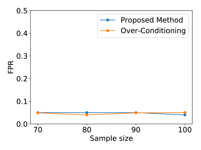
(a) FPR

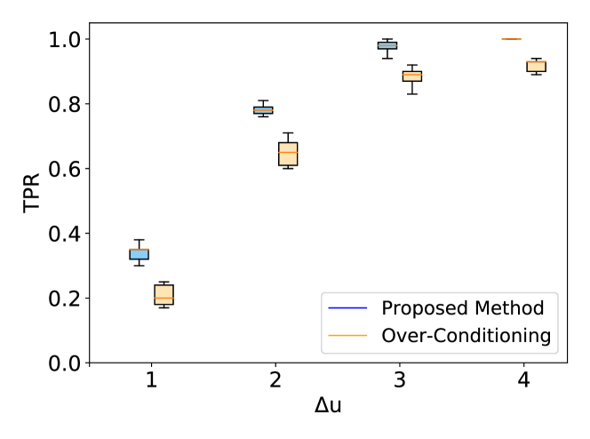
(b) TPR

Figure 2: Results of FPR and TPR for fused lasso.

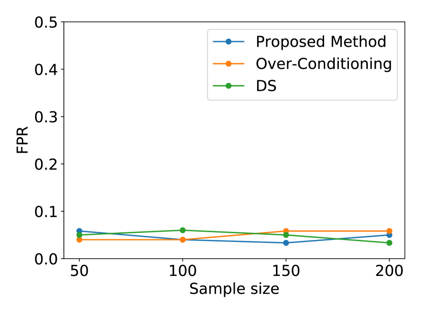
(c) FPR

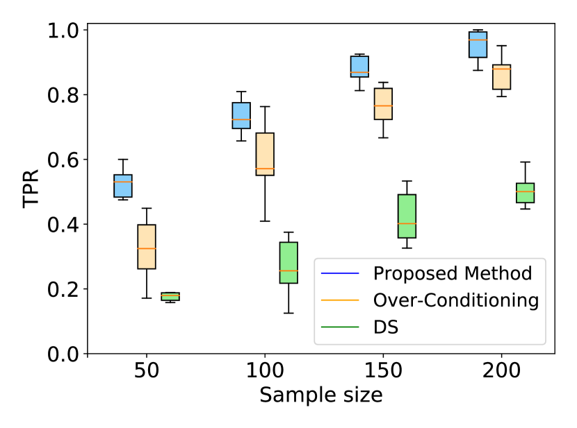
(d) TPR

(e) CI

Figure 3: Results of FPR, TPR, and CI for vanilla lasso.

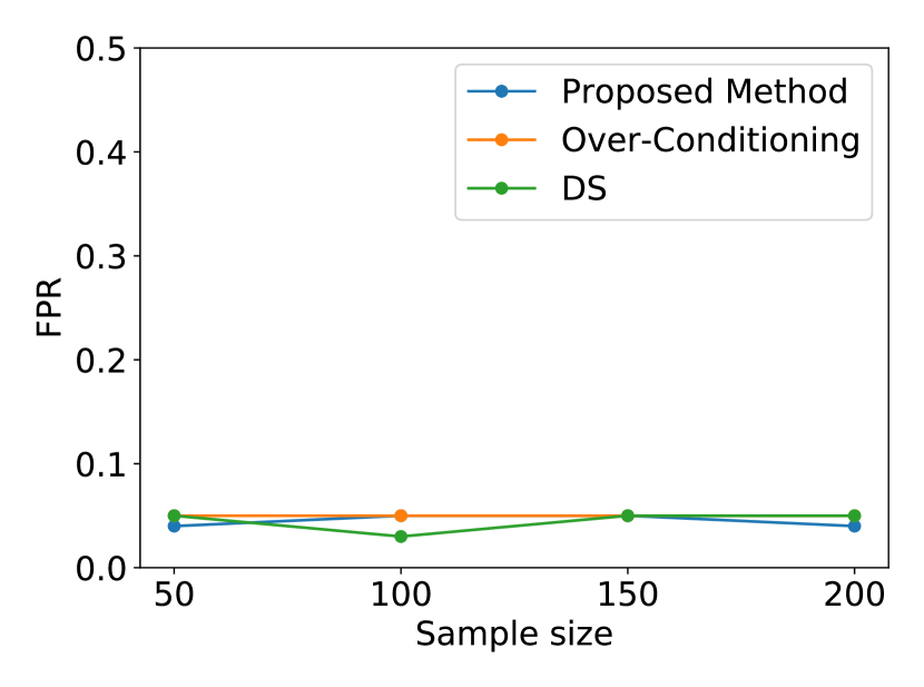
(a) FPR

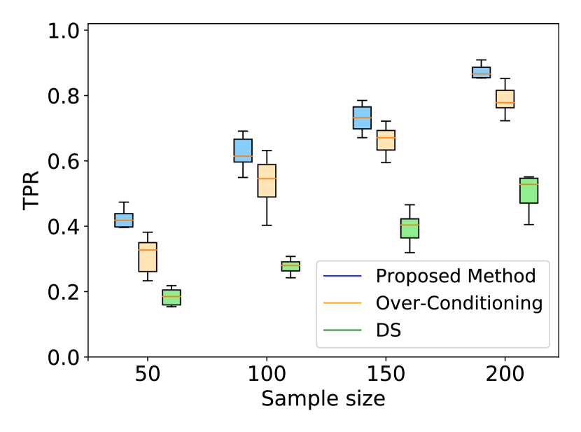
(b) TPR

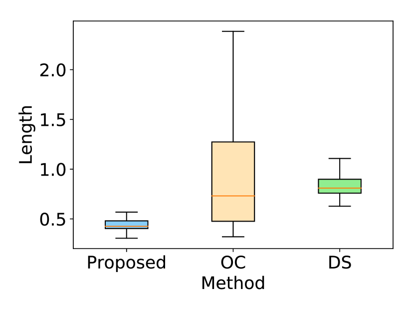
(c) CI

Figure 4: Results of FPR, TPR, and CI for elastic net.

Definition of TPR.

In SI, statistical testing is only conducted when at least one hypothesis is discovered by the algorithm. Therefore, the definition of the TPR, which is also known as the conditional power, is as follows:

$${\rm TPR}=\frac{{\rm\#\ correctly~{}detected\ \&\ rejected}}{{\rm\#\ correctly~{}detected}}.$$

In the case of fused lasso, a detection is considered as correct if it is within $L=\pm 2$ of the true CP locations. This is because it is often difficult to identify the exact CPs accurately in the presence of noise. Many existing studies considered a detection to be correct if it was within $L$ positions of the true CP locations (Truong et al., 2020). In the case of feature selection, ${\rm\#\ correctly~{}detected}$ indicates the number of truly positive features that are selected by the algorithm (e.g., lasso), whereas ${\rm\#\ rejected}$ indicates the number of truly positive features for which the null hypothesis is rejected by the SI.

6.2 Numerical Results

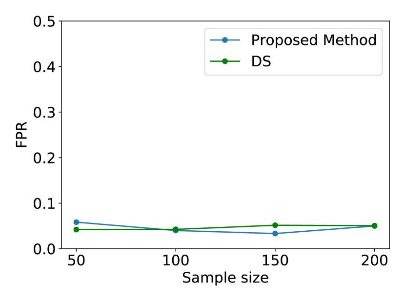
(a) FPR

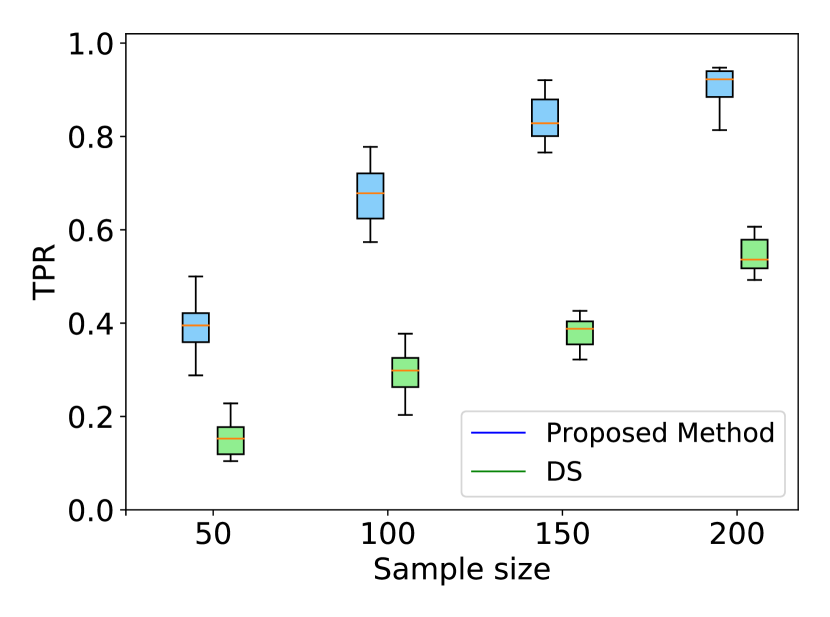
(b) TPR

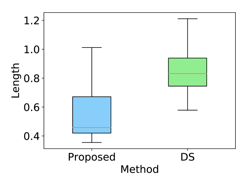
(c) CI

Figure 5: Results of FPR, TPR, and CI for non-negative least squares.

FPR, TPR, and CI results.

The fused lasso results are presented in Figure 4. The results for the vanilla lasso, elastic net, non-negative least squares, and Huber regression + $\ell_{1}$ norm are depicted in Figures 4, 4, 5, and 6, respectively. No over-conditioning occurred in the case of the non-negative least squares as we had already restricted the coefficients to be positive. In summary, although all of the methods could properly control the FPR at a significance level of $\alpha$, the proposed method had the highest power among the methods. The CI results were also consistent with the TPR results. That is, the shortest CI for the proposed method indicated that it exhibited the highest power.

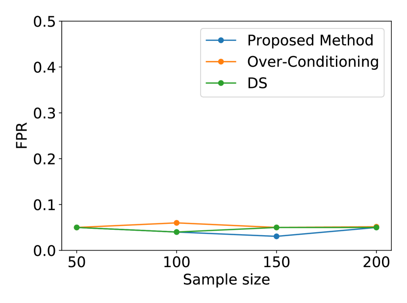
(a) FPR

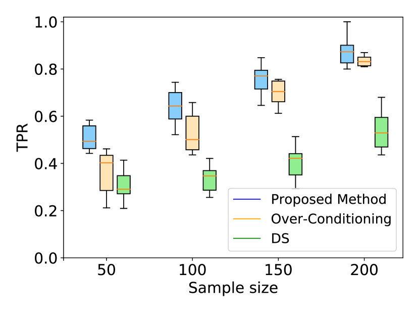
(b) TPR

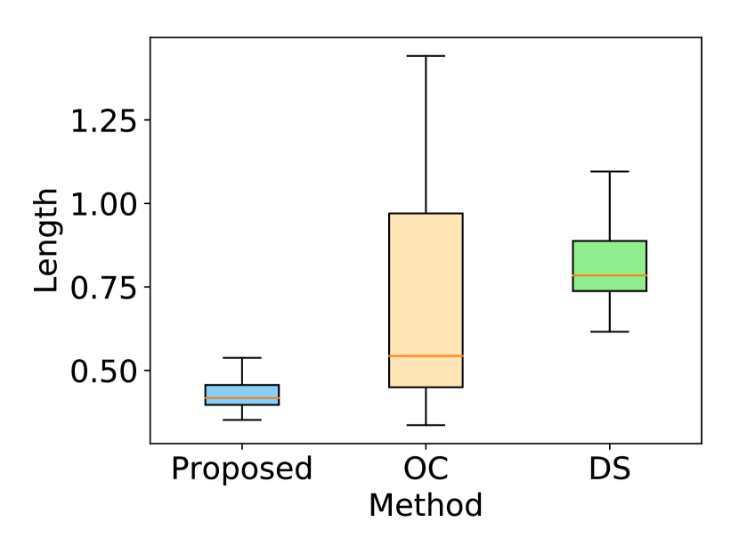
(c) CI

Figure 6: FPR, TPR, and CI results for Huber regression with $\ell_{1}$ penalty.

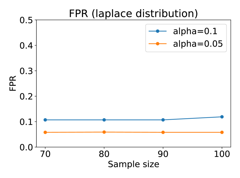
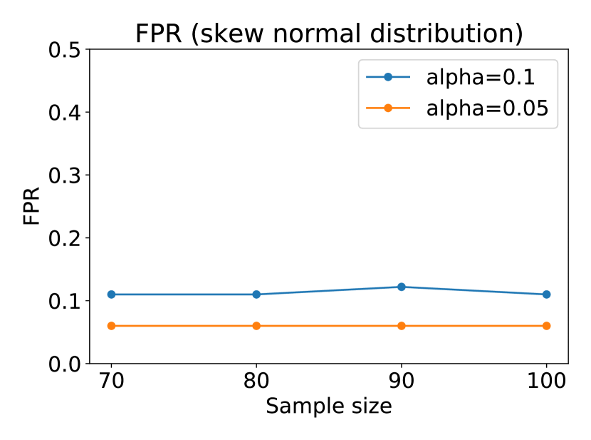
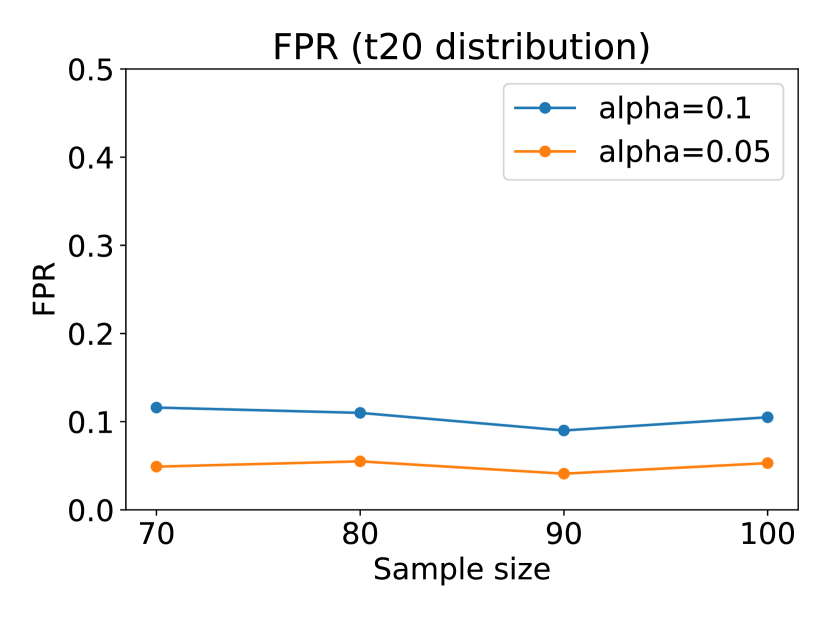
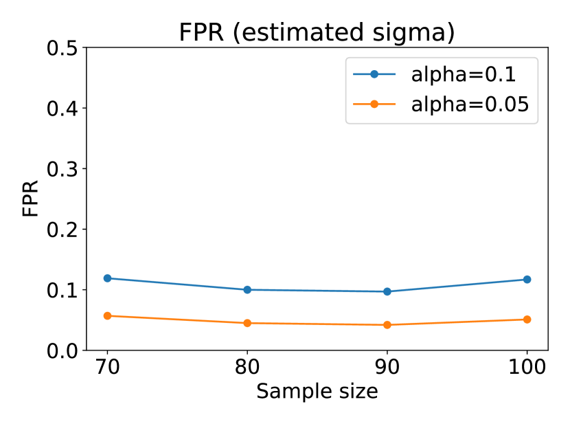
Figure 7: Robustness of proposed method for fused lasso.

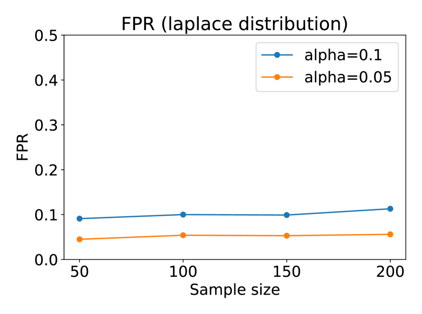
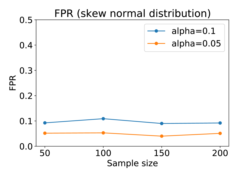
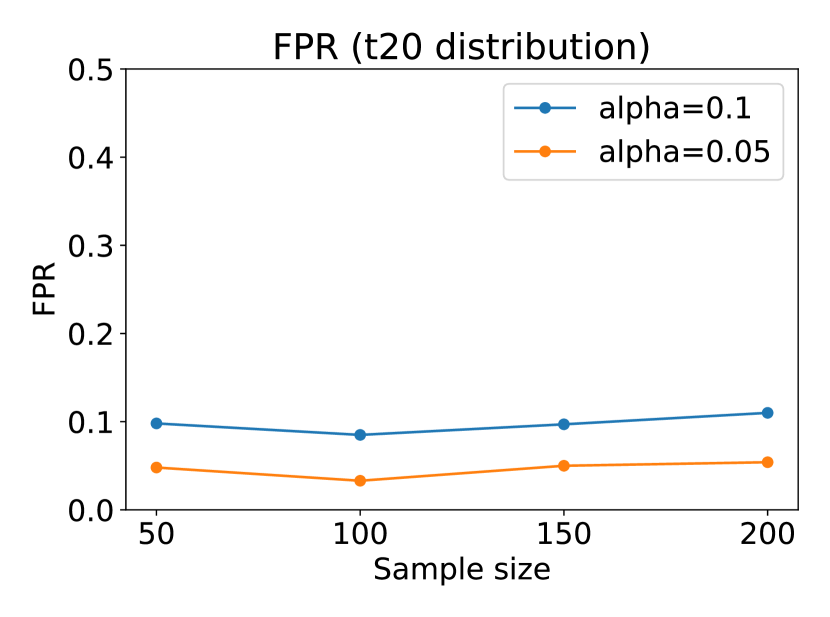
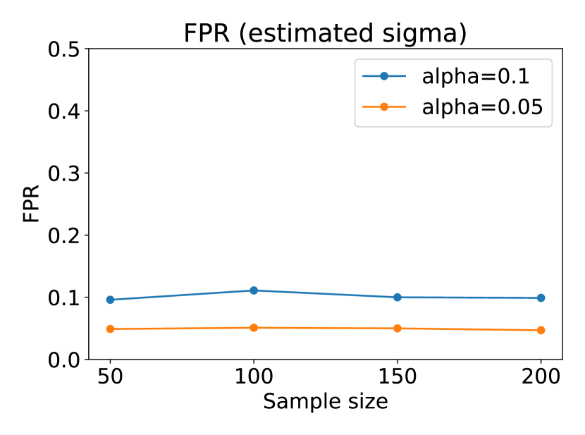
Figure 8: Robustness of proposed method for vanilla lasso.

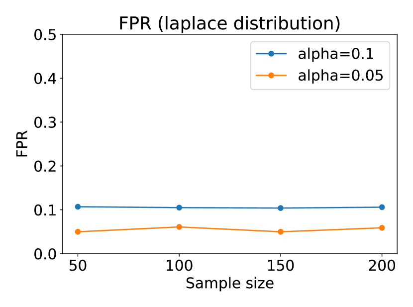
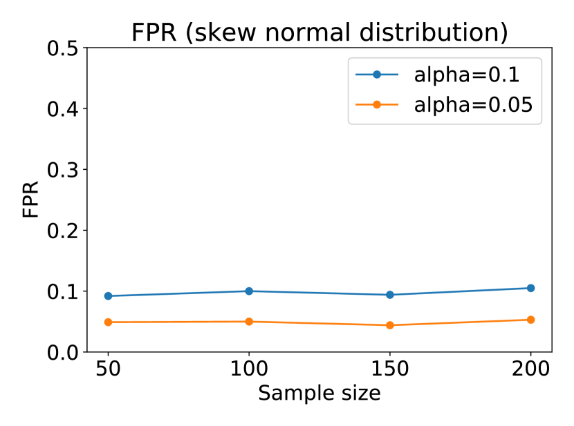
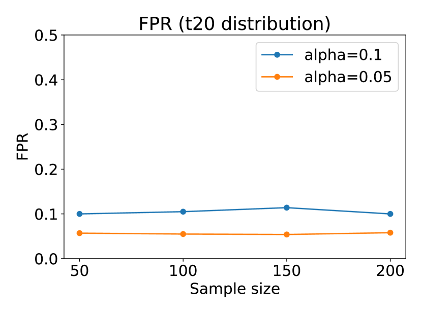
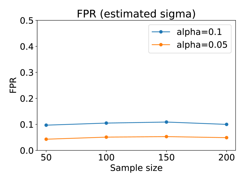
Figure 9: Robustness of proposed method for elastic net.

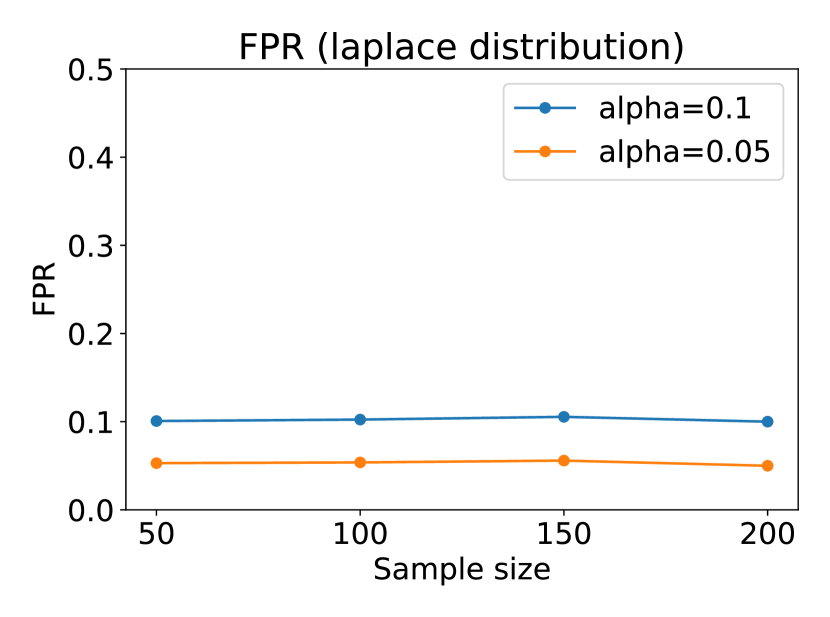
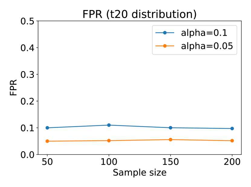
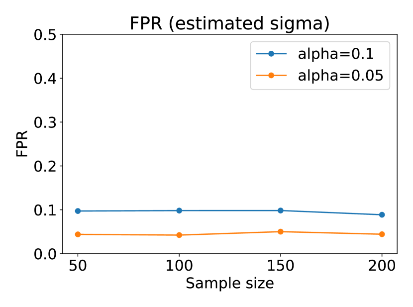
Figure 10: Robustness of proposed method for non-negative least squares.

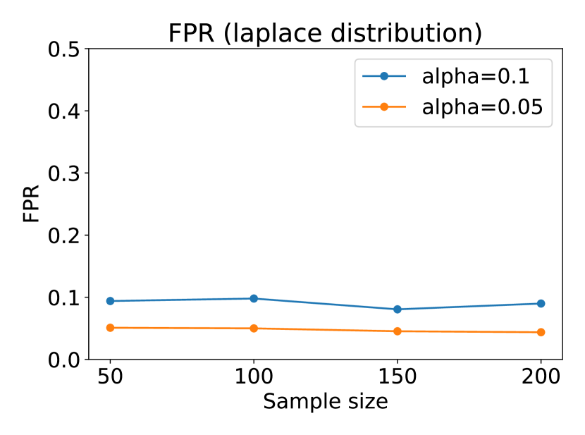
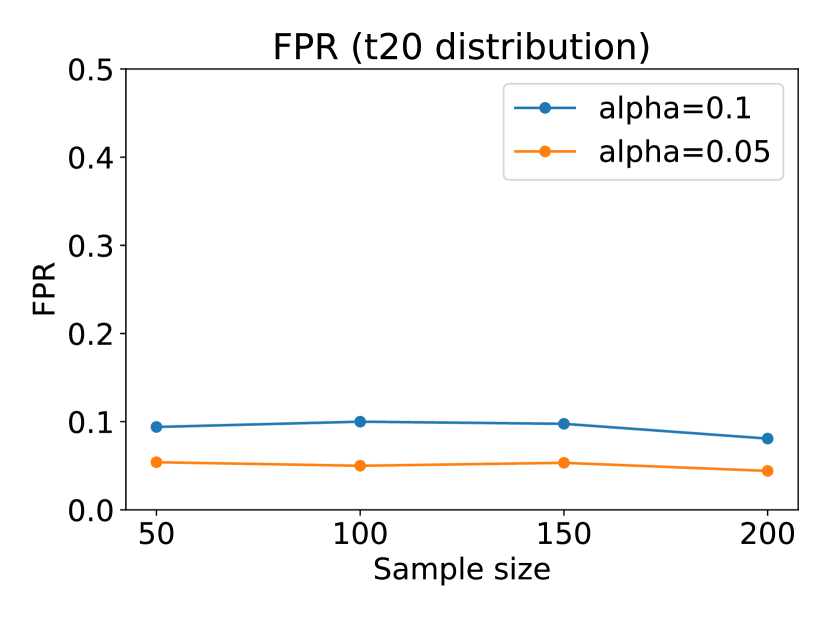
Figure 11: Robustness of proposed method for Huber regression with $\ell_{1}$ penalty.

Robustness of proposed method in terms of FPR control.

We demonstrated the robustness of our method in terms of FPR control by considering the following cases:

$\bullet$ Non-normal noise: We considered the noise following the Laplace distribution, skew normal distribution (skewness coefficient: 10), and $t_{20}$ distribution.

$\bullet$ Unknown $\sigma^{2}$: We considered the case in which the variance was estimated from the data.

We generated $n$ outcomes: $y_{i}=\bm{x}_{i}^{\top}\bm{\beta}+\varepsilon_{i}$, $i=1,...,n$, where $p=5,\bm{x}_{i}\sim\mathbb{N}(0,I_{p})$, and $\varepsilon_{i}$ follows a Laplace distribution, skew normal distribution, or $t_{20}$ distribution with a zero mean and the standard deviation set to 1. In the case of the estimated $\sigma^{2}$, $\varepsilon_{i}\sim\mathbb{N}(0,1)$. We set all elements of $\bm{\beta}$ to 0 and set $\lambda=0.5$. For every case, we ran 1,200 trials for each $n\in\{50,100,150,200\}$. We confirmed that our method maintained high performance on FPR control. The results are presented in Figures 10, 10, 10, 10, and 11.

Results when accounting for CV selection event.

We conducted a comparison of the TPRs between the proposed method and the OC version that was proposed in Loftus (2015) when $\lambda$ was selected from $\Lambda_{1}=\{2^{-1},2^{0},2^{1}\}$ or $\Lambda_{2}=\{2^{-10},2^{-9},...,2^{9},2^{10}\}$. The results are presented in Figure 12. The existing method had lower power because additional conditioning on all intermediate models was required, which was also discussed in Markovic et al. (2017). Our method exhibited higher power as we could characterize the minimum conditioning amount.

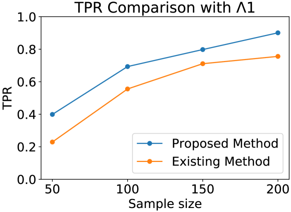
(a) $\Lambda_{1}=\{2^{-1},2^{0},2^{1}\}$

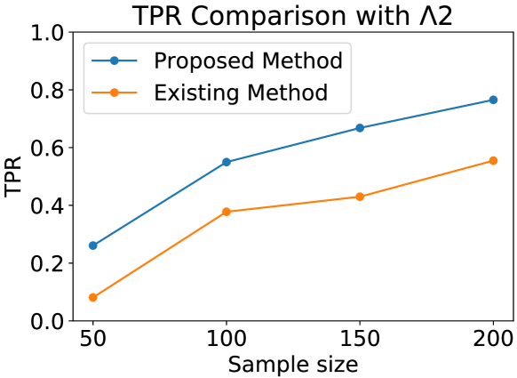
(b) $\Lambda_{2}=\{2^{-10},...,2^{10}\}$

Figure 12: TPR comparison with existing method (Loftus, 2015) when accounting for CV selection event.

Efficiency of proposed method.

Our main purpose was to demonstrate that the proposed method has not only high statistical power, but also reasonable computational costs. We conducted experiments on feature selection by lasso. The computational time of the proposed method was almost linear with respect to the number of active features, as illustrated in Figure 13(a). Figure 13(b) presents a boxplot of the actual number of intervals of z that were encountered on the line when constructing the truncation region ${\mathcal{Z}}$. Figure 13(c) depicts the efficiency of our method compared to that of Lee et al. (2016), in which the authors mentioned the naive method for removing sign conditioning by enumerating all possible combinations of signs $2^{|{\mathcal{M}}_{\rm obs}|}$.

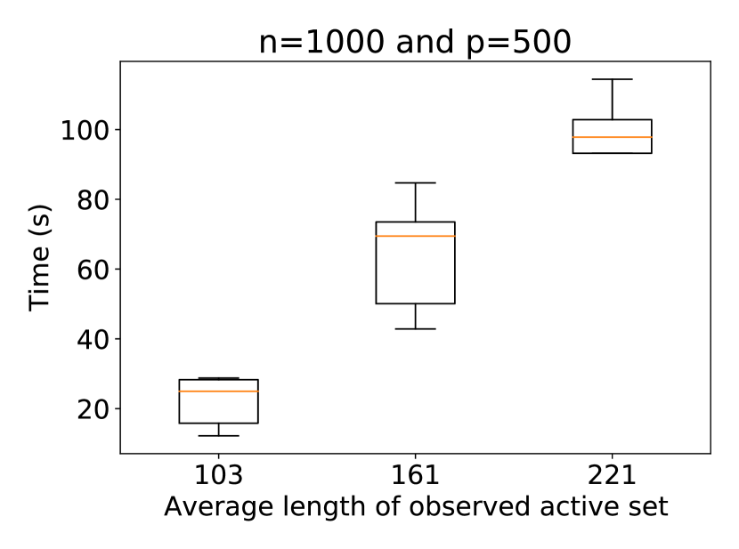
(a) Computational time of proposed method.

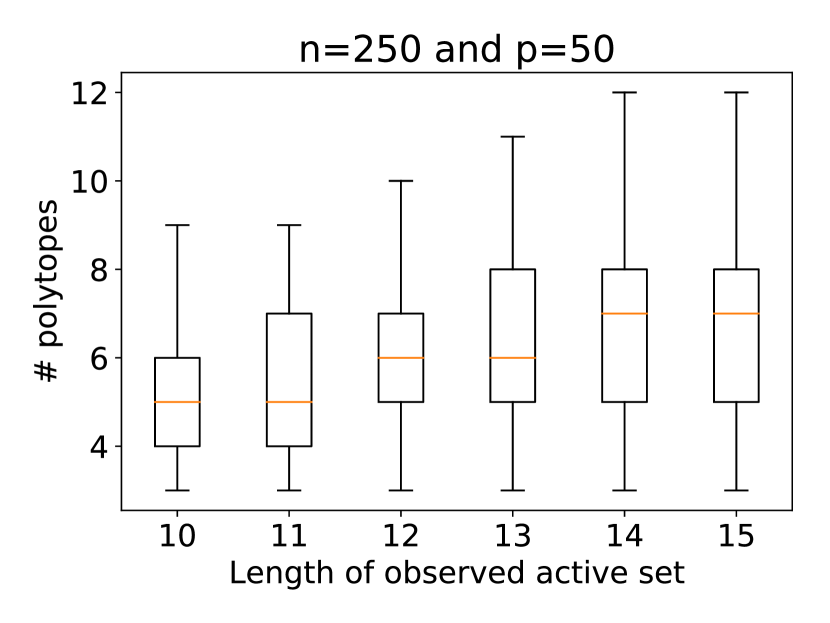
(b) Number of encountered intervals on line.

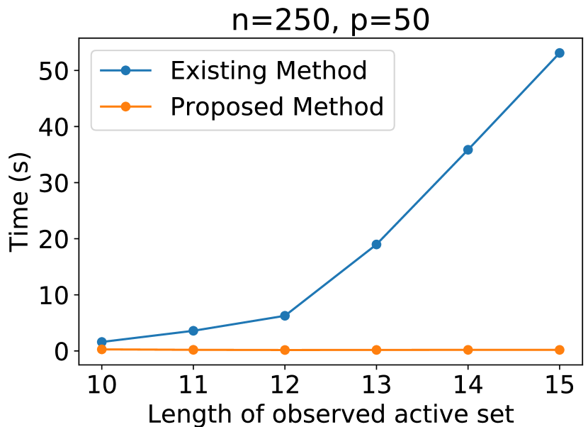
(c) Comparison with Lee et al. (2016).

Figure 13: Efficiency of proposed method.

Comparison with Liu et al. (2018).

Furthermore, we demonstrated the efficiency of our method compared to the two methods proposed in §3 (inference for partial regression targets) of Liu et al. (2018). In this work, only stable features were allowed to influence the formation of the test statistic. Stable features are those with very strong signals and that cannot missed. In the first method, which we refer to as TN-$\ell_{1}$, the stable features were selected by setting a higher value of $\lambda$. In the second method, which we refer to as TN-Custom, the stable features were selected by setting a cutoff value. The details of these two methods are presented in Appendix B. In general, to perform SI with these two methods, all possible combinations of signs, which increase exponentially, still need to be naively enumerated. The proposed method can be used to solve this computational bottleneck. A comparison of the computational costs is illustrated in Figure 14.

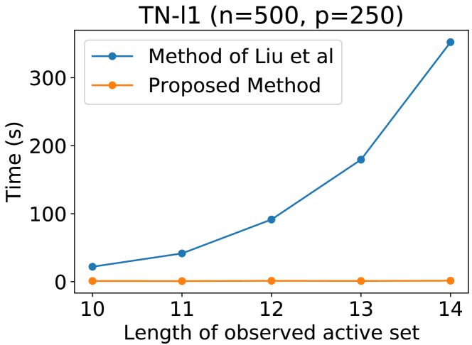
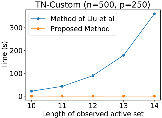
Figure 14: Comparison between proposed method and methods in Liu et al. (2018), in which an exponentially increasing number of all possible sign combinations is still required.

6.3 Results on Real-World Datasets

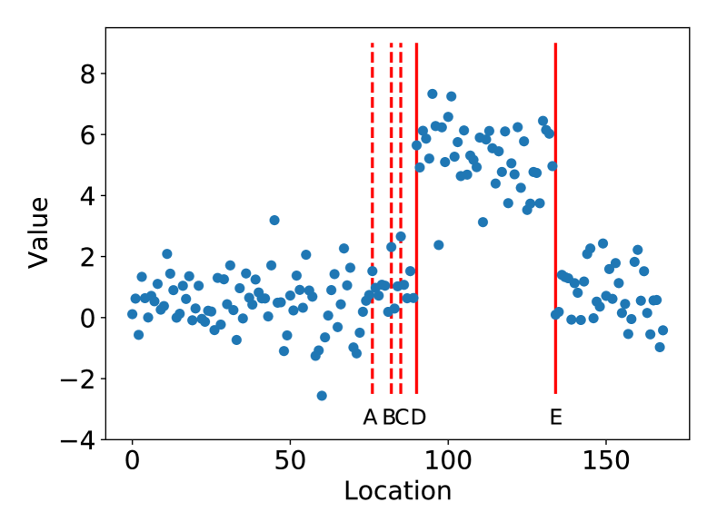
	A	B	C	D	E
Proposed	0.9	0.6	0.3	$1.4\times 10^{-15}$	0.0
OC	0.9	0.3	0.3	$6.0\times 10^{-5}$	$1.2\times 10^{-11}$

(a) Chromosomes 17, 18, and 19.

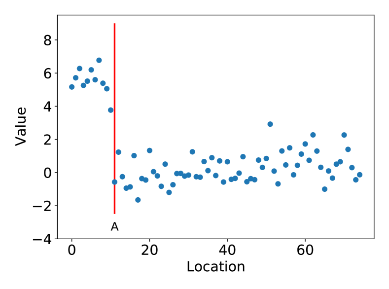
	A
Proposed	$~{}~{}~{}~{}~{}~{}~{}~{}~{}0.0~{}~{}~{}~{}~{}~{}~{}~{}~{}$
OC	0.0

(b) Chromosome 14.

Figure 15: Experimental results for cell lines GM00143 and GM01750.

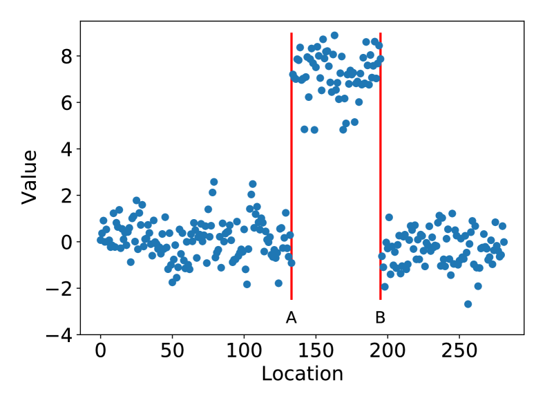
	A	B
Proposed	$~{}~{}2.7\times 10^{-320}~{}~{}$	$~{}~{}~{}~{}~{}0.0~{}~{}~{}~{}~{}$
OC	$5.3\times 10^{-98}$	0.0

(c) Chromosomes 1, 2, and 3.

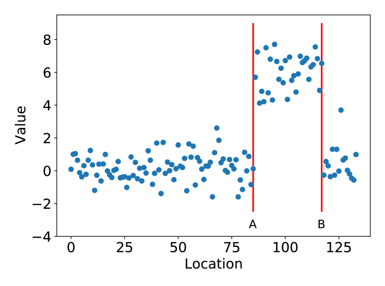
	A	B
Proposed	$~{}~{}1.1\times 10^{-41}~{}~{}$	$~{}~{}9.1\times 10^{-14}~{}~{}$
OC	$1.1\times 10^{-41}$	$9.1\times 10^{-14}$

(d) Chromosomes 20, 21, and 22.

Figure 16: Experimental results for cell line GM03576.

Array CGH data.

Array CGH analyses enable the detection of changes in copy numbers across the genome. We applied the proposed method and OC to the dataset with the ground truth provided in Snijders et al. (2001). The results of the detected CPs and tables of $p$-values are presented in Figures 16 and 16. The solid red line denotes the significant CPs, which had a $p$-value that was smaller than the significance level following Bonferroni correction. All of the results were consistent with those of Snijders et al. (2001). Moreover, we compared the $p$-values of the proposed method and OC. The $p$-values of the proposed method were smaller than or equal to those of OC for all true CPs, which indicates that the proposed method had higher power than OC.

The boxplots of the distribution of the $p$-values for the proposed method and OC on the real-world dataset are illustrated in Figure 17. We used the jointseg package (Pierre-Jean et al., 2014) to generate realistic DNA copy number profiles of cancer samples with “known” truths. Two datasets consisting of 1,000 profiles, each with a length of $n=60$, were created, as follows:

• Dataset 1: Resampled from GSE11976 with tumor fraction $=$ 1.

• Dataset 2: Resampled from GSE29172 with tumor fraction $=$ 1.

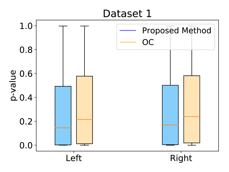
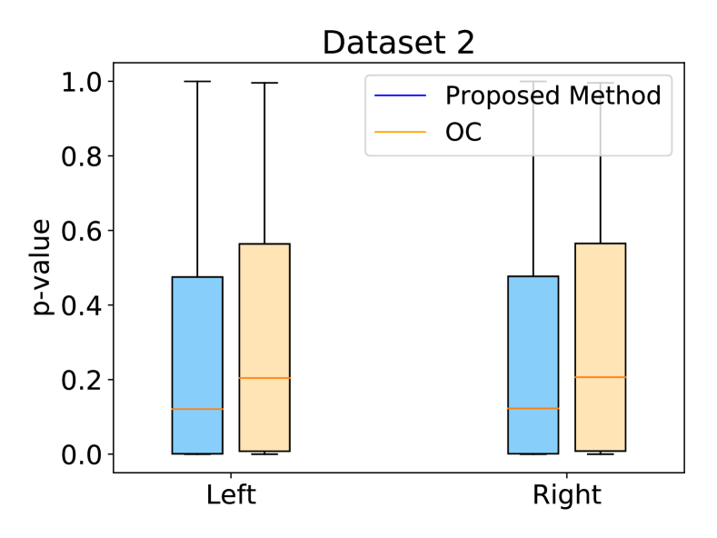
Figure 17: Boxplots of $p$-values. The left plot in each figure depicts the distributions of the $p$-values, whereas the right plot displays the distributions of the $p$-values for the cases in which the two $p$-values of the proposed method and OC differed. In Dataset 1, the percentage of the $p$-value of the proposed method was 55.81% smaller than that of OC. In Dataset 2, the percentage of the $p$-value of the proposed method was 54.24% smaller than that of OC. In general, the $p$-value of the proposed method tended to be smaller than that of OC, which indicates that the proposed method had higher statistical power than OC.

Nile data.

These data contain the annual flow volume of the Nile River at Aswan from 1871 to 1970 (100 years). In this case, the interest lies in unexpected events such as natural disasters. According to Figure 18, the proposed algorithm identified a CP at the $28^{\rm th}$ position, corresponding to the year 1899. This result was consistent with that of Jung et al. (2017).

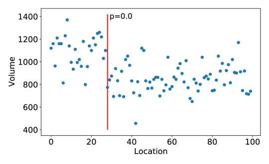
Figure 18: Experimental result for Nile data. A CP was detected at the $28^{\rm th}$ position, which indicates that a change in the volume level occurred in 1899.

Prostate data.

We applied our proposed method for lasso to the prostate dataset from Hastie et al. (2009). As $p<n$ for this dataset, we could estimate $\sigma^{2}$ using the residual sum of squares from the full regression model with all $p$ predictors. We set $\lambda=5$. Figure 19 depicts the 95% CIs for the features that were selected by both lasso and DS.

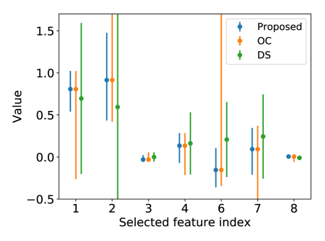
Figure 19: Experimental results for prostate data. The indices of the features were 1: lcavol, 2: lweight, 3: age, 4: lbph, 6: lcp, 7: gleason, and 8: pgg45.

Acknowledgements

This work was partially supported by MEXT KAKENHI (20H00601, 16H06538), JST Moonshot R&D (JPMJMS2033-05), NEDO (JPNP18002, JPNP20006), RIKEN Center for Advanced Intelligence Project, and RIKEN Junior Research Associate Program.

Appendix A Full Target Case for Lasso in Liu et al. [2018]

In the full target case, as discussed in Liu et al. [2018], the data are used to select the interesting features, but they are not used to summarize the relation between the response and the selected features. Therefore, all features can be used to define the direction of interest.

$$\bm{\eta}_{j}=X(X^{\top}X)^{-1}\bm{e}_{j},$$

where $\bm{e}_{j}\in\mathbb{R}^{p}$ is a zero vector with 1 at the $j^{\rm th}$ coordinate. The conditional inference is defined as

$$\bm{\eta}_{j}^{\top}\bm{\bm{Y}}\mid\left\{j\in{\mathcal{A}}(\bm{Y}),\bm{q}(\bm{Y})=\bm{q}({\bm{y}}^{\rm obs})\right\}.$$ (45)

In Liu et al. [2018], the authors proposed a solution for conducting conditional inference for a specific case when $p<n$, and there was no solution for the case when $p>n$. This problem can be solved with the proposed PP method. First, we rewrite the conditional inference in (45) as the problem of characterizing the sampling distribution of

$$Z\mid\{Z\in{\mathcal{Z}}\}\text{ where }{\mathcal{Z}}=\{z\in\mathbb{R}\mid j\in{\mathcal{A}}(\bm{y}(z))\}.$$ (46)

$\bm{y}(z)$ in (46) is defined as in (15). Thereafter, to identify ${\mathcal{Z}}$, only the path of the lasso solution $\hat{\bm{\beta}}(z)$ needs to be obtained, as proposed in §3, and the intervals in which $j$ is an element of the active set corresponding to $\hat{\bm{\beta}}(z)$ simply need to be verified along the path. Finally, after obtaining ${\mathcal{Z}}$, we can easily compute the selective $p$-value or selective CI.

Appendix B Stable Partial Target Case for Lasso in Liu et al. [2018]

In the stable partial target case, as discussed in Liu et al. [2018], only stable features are allowed to influence the formation of the test statistic. Stable features are those with very strong signals that we do not wish to omit. We select a set ${\mathcal{H}}_{\rm obs}$ of stable features. Subsequently, for any $j\in{\mathcal{H}}_{\rm obs},j\in{\mathcal{M}}_{\rm obs}$,

$$\bm{\eta}_{j}=X_{{\mathcal{H}}_{\rm obs}}(X_{{\mathcal{H}}_{\rm obs}}^{\top}X_{{\mathcal{H}}_{\rm obs}})^{-1}\bm{e}_{j}.$$

For any $j\not\in{\mathcal{H}}_{\rm obs},j\in{\mathcal{M}}_{\rm obs}$,

$$\bm{\eta}_{j}=X_{{\mathcal{H}}_{\rm obs}\cup\{j\}}(X_{{\mathcal{H}}_{\rm obs}\cup\{j\}}^{\top}X_{{\mathcal{H}}_{\rm obs}\cup\{j\}})^{-1}\bm{e}_{j}.$$

Next, we demonstrate how to construct ${\mathcal{H}}_{\rm obs}$ according to Liu et al. [2018].

Stable target formation by setting higher value of $\lambda$ (TN-$\ell_{1}$).

In this case, ${\mathcal{H}}_{\rm obs}$ is the lasso active set, but with a higher value of $\lambda$ than that used to select ${\mathcal{M}}_{\rm obs}$. We denote ${\mathcal{H}}_{\rm obs}={\mathcal{H}}({\bm{y}}^{\rm obs})$, and subsequently, the conditional inference is defined as

$$\bm{\eta}_{j}^{\top}\bm{\bm{Y}}\mid\left\{j\in{\mathcal{A}}(\bm{Y}),{\mathcal{H}}(\bm{Y})={\mathcal{H}}({\bm{y}}^{\rm obs}),\bm{q}(\bm{Y})=\bm{q}({\bm{y}}^{\rm obs})\right\}.$$ (47)

The main drawback of the method in Liu et al. [2018] is that all $2^{|{\mathcal{H}}_{\rm obs}|}$ sign vectors must be considered, which requires substantial computation time when $|{\mathcal{H}}_{\rm obs}|$ is large. This limitation can easily be overcome using our piecewise linear homotopy computation. First, we rewrite the conditional inference in (47) as the problem of characterizing the sampling distribution of

$$Z\mid\{Z\in{\mathcal{Z}}\}\text{ where }{\mathcal{Z}}=\{z\in\mathbb{R}\mid j\in{\mathcal{A}}(\bm{y}(z)),{\mathcal{H}}(\bm{y}(z))={\mathcal{H}}({\bm{y}}^{\rm obs})\}.$$

Thereafter, we can easily identify ${\mathcal{Z}}={\mathcal{Z}}_{1}\cap{\mathcal{Z}}_{2}$, where ${\mathcal{Z}}_{1}=\{z\in\mathbb{R}\mid j\in{\mathcal{A}}(\bm{y}(z))\}$ and ${\mathcal{Z}}_{2}=\{z\in\mathbb{R}\mid{\mathcal{H}}(\bm{y}(z))={\mathcal{H}}({\bm{y}}^{\rm obs})\}$, which we can simply obtain using the method proposed in §3 of the main paper.

Stable target formation by setting cutoff value $c$ (TN-Custom).

In this case, we determine ${\mathcal{H}}_{\rm obs}$ by setting a cutoff value $c$ to select $\beta_{j}$, such that $|\beta_{j}|\geq c$ . The set ${\mathcal{H}}_{\rm obs}$ is defined as

$${\mathcal{H}}_{\rm obs}=\left\{j\in{\mathcal{M}}_{\rm obs},|\beta_{j}|\geq c\right\},$$

where $\beta_{j}=\bm{e}^{\top}_{j}(X_{{\mathcal{M}}_{\rm obs}}^{\top}X_{{\mathcal{M}}_{\rm obs}})^{-1}X_{{\mathcal{M}}_{\rm obs}}^{\top}\bm{y}^{\rm obs}$. We denote ${\mathcal{H}}_{\rm obs}={\mathcal{H}}({\mathcal{M}}_{\rm obs})\subset{\mathcal{M}}_{\rm obs}$, and subsequently, the conditional inference is formulated as

$$\bm{\eta}_{j}^{\top}\bm{Y}\mid\left\{{\mathcal{H}}({\mathcal{A}}(\bm{Y}))={\mathcal{H}}({\mathcal{M}}_{\rm obs}),{\mathcal{A}}(\bm{Y})={\mathcal{M}}_{\rm obs}\right\}.$$ (48)

The main drawback of the method in Liu et al. [2018] is that it still requires conditioning on $\{{\mathcal{A}}(\bm{Y})={\mathcal{M}}_{\rm obs}\}$, which is computationally intractable when $|{\mathcal{M}}_{\rm obs}|$ is large, because the enumeration of $2^{|{\mathcal{M}}_{\rm obs}|}$ sign vectors is required. This limitation can easily be overcome using our proposed method.

References

- Ali and Tibshirani [2019] A. Ali and R. J. Tibshirani. The generalized lasso problem and uniqueness. Electronic Journal of Statistics, 13(2):2307–2347, 2019.
- Allgower and George [1993] E. L. Allgower and K. George. Continuation and path following. Acta Numerica, 2:1–63, 1993.
- Bach et al. [2006] F. R. Bach, D. Heckerman, and E. Horvits. Considering cost asymmetry in learning classifiers. Journal of Machine Learning Research, 7:1713–41, 2006.
- Benjamini and Yekutieli [2005] Y. Benjamini and D. Yekutieli. False discovery rate–adjusted multiple confidence intervals for selected parameters. Journal of the American Statistical Association, 100(469):71–81, 2005.
- Benjamini et al. [2009] Y. Benjamini, R. Heller, and D. Yekutieli. Selective inference in complex research. Philosophical Transactions of the Royal Society A: Mathematical, Physical and Engineering Sciences, 367(1906):4255–4271, 2009.
- Berk et al. [2013] R. Berk, L. Brown, A. Buja, K. Zhang, and L. Zhao. Valid post-selection inference. The Annals of Statistics, 41(2):802–837, 2013.
- Best [1996] M. J. Best. An algorithm for the solution of the parametric quadratic programming problem. Applied Mathemetics and Parallel Computing, pages 57–76, 1996.
- Chen and Bien [2019] S. Chen and J. Bien. Valid inference corrected for outlier removal. Journal of Computational and Graphical Statistics, pages 1–12, 2019.
- Choi et al. [2017] Y. Choi, J. Taylor, and R. Tibshirani. Selecting the number of principal components: Estimation of the true rank of a noisy matrix. The Annals of Statistics, 45(6):2590–2617, 2017.
- Cox [1975] D. R. Cox. A note on data-splitting for the evaluation of significance levels. Biometrika, 62(2):441–444, 1975.
- Duy et al. [2020a] V. N. L. Duy, S. Iwazaki, and I. Takeuchi. Quantifying statistical significance of neural network representation-driven hypotheses by selective inference. arXiv preprint arXiv:2010.01823, 2020a.
- Duy et al. [2020b] V. N. L. Duy, H. Toda, R. Sugiyama, and I. Takeuchi. Computing valid p-value for optimal changepoint by selective inference using dynamic programming. In Advances in Neural Information Processing Systems, 2020b.
- Efron and Tibshirani [2004] B. Efron and R. Tibshirani. Least angle regression. Annals of Statistics, 32(2):407–499, 2004.
- Fithian et al. [2014] W. Fithian, D. Sun, and J. Taylor. Optimal inference after model selection. arXiv preprint arXiv:1410.2597, 2014.
- Fithian et al. [2015] W. Fithian, J. Taylor, R. Tibshirani, and R. Tibshirani. Selective sequential model selection. arXiv preprint arXiv:1512.02565, 2015.
- Gal [1995] T. Gal. Postoptimal Analysis, Parametric Programming, and Related Topics. Walter de Gruyter, 1995.
- Hastie et al. [2004] T. Hastie, S. Rosset, R. Tibshirani, and J. Zhu. The entire regularization path for the support vector machine. Journal of Machine Learning Research, 5:1391–415, 2004.
- Hastie et al. [2009] T. Hastie, R. Tibshirani, and J. Friedman. The elements of statistical learning: data mining, inference, and prediction. Springer Science & Business Media, 2009.
- Hocking et al. [2011] T. Hocking, j. P. Vert, F. Bach, and A. Joulin. Clusterpath: an algorithm for clustering using convex fusion penalties. In Proceedings of the 28th International Conference on Machine Learning, pages 745–752, 2011.
- Huber [1992] P. J. Huber. Robust estimation of a location parameter. In Breakthroughs in statistics, pages 492–518. Springer, 1992.
- Hyun et al. [2018a] S. Hyun, M. G’sell, and R. J. Tibshirani. Exact post-selection inference for the generalized lasso path. Electronic Journal of Statistics, 12(1):1053–1097, 2018a.
- Hyun et al. [2018b] S. Hyun, K. Lin, M. G’Sell, and R. J. Tibshirani. Post-selection inference for changepoint detection algorithms with application to copy number variation data. arXiv preprint arXiv:1812.03644, 2018b.
- Jung et al. [2017] M. Jung, S. Song, and Y. Chung. Bayesian change-point problem using bayes factor with hierarchical prior distribution. Communications in Statistics-Theory and Methods, 46(3):1352–1366, 2017.
- Karasuyama and Takeuchi [2010] M. Karasuyama and I. Takeuchi. Nonlinear regularization path for quadratic loss support vector machines. IEEE Transactions on Neural Networks, 22(10):1613–1625, 2010.
- Karasuyama et al. [2012] M. Karasuyama, N. Harada, M. Sugiyama, and I. Takeuchi. Multi-parametric solution-path algorithm for instance-weighted support vector machines. Machine Learning, 88(3):297–330, 2012.
- Le Duy and Takeuchi [2021] V. N. Le Duy and I. Takeuchi. Parametric programming approach for more powerful and general lasso selective inference. In International Conference on Artificial Intelligence and Statistics, pages 901–909. PMLR, 2021.
- Lee and Scott [2007] G. Lee and C. Scott. The one class support vector machine solution path. In Proc. of ICASSP 2007, pages II521–II524, 2007.
- Lee et al. [2016] J. D. Lee, D. L. Sun, Y. Sun, and J. E. Taylor. Exact post-selection inference, with application to the lasso. The Annals of Statistics, 44(3):907–927, 2016.
- Leeb and Pötscher [2005] H. Leeb and B. M. Pötscher. Model selection and inference: Facts and fiction. Econometric Theory, pages 21–59, 2005.
- Leeb and Pötscher [2006] H. Leeb and B. M. Pötscher. Can one estimate the conditional distribution of post-model-selection estimators? The Annals of Statistics, 34(5):2554–2591, 2006.
- Liu et al. [2018] K. Liu, J. Markovic, and R. Tibshirani. More powerful post-selection inference, with application to the lasso. arXiv preprint arXiv:1801.09037, 2018.
- Lockhart et al. [2014] R. Lockhart, J. Taylor, R. J. Tibshirani, and R. Tibshirani. A significance test for the lasso. Annals of statistics, 42(2):413, 2014.
- Loftus [2015] J. R. Loftus. Selective inference after cross-validation. arXiv preprint arXiv:1511.08866, 2015.
- Loftus and Taylor [2014] J. R. Loftus and J. E. Taylor. A significance test for forward stepwise model selection. arXiv preprint arXiv:1405.3920, 2014.
- Mairal and Yu [2012] J. Mairal and B. Yu. Complexity analysis of the lasso regularization path. arXiv preprint arXiv:1205.0079, 2012.
- Markovic et al. [2017] J. Markovic, L. Xia, and J. Taylor. Unifying approach to selective inference with applications to cross-validation. arXiv preprint arXiv:1703.06559, 2017.
- Ogawa et al. [2013] K. Ogawa, M. Imamura, I. Takeuchi, and M. Sugiyama. Infinitesimal annealing for training semi-supervised support vector machines. In International Conference on Machine Learning, pages 897–905, 2013.
- Osborne et al. [2000] M. R. Osborne, B. Presnell, and B. A. Turlach. A new approach to variable selection in least squares problems. IMA journal of numerical analysis, 20(3):389–403, 2000.
- Panigrahi et al. [2016] S. Panigrahi, J. Taylor, and A. Weinstein. Bayesian post-selection inference in the linear model. arXiv preprint arXiv:1605.08824, 28, 2016.
- Pierre-Jean et al. [2014] M. Pierre-Jean, G. Rigaill, and P. Neuvial. Performance evaluation of dna copy number segmentation methods. Briefings in bioinformatics, 16(4):600–615, 2014.
- Pötscher and Schneider [2010] B. M. Pötscher and U. Schneider. Confidence sets based on penalized maximum likelihood estimators in gaussian regression. Electronic Journal of Statistics, 4:334–360, 2010.
- Ritter [1984] K. Ritter. On parametric linear and quadratic programming problems. mathematical Programming: Proceedings of the International Congress on Mathematical Programming, pages 307–335, 1984.
- Rosset and Zhu [2007] S. Rosset and J. Zhu. Piecewise linear regularized solution paths. Annals of Statistics, 35:1012–1030, 2007.
- She and Owen [2011] Y. She and A. B. Owen. Outlier detection using nonconvex penalized regression. Journal of the American Statistical Association, 106(494):626–639, 2011.
- Snijders et al. [2001] A. M. Snijders, N. Nowak, R. Segraves, S. Blackwood, N. Brown, J. Conroy, G. Hamilton, A. K. Hindle, B. Huey, and K. Kimura. Assembly of microarrays for genome-wide measurement of dna copy number. Nature genetics, 29(3):263, 2001.
- Sugiyama et al. [2020] K. Sugiyama, V. N. L. Duy, and I. Takeuchi. More powerful and general selective inference for stepwise feature selection using the homotopy continuation approach. arXiv preprint arXiv:2012.13545, 2020.
- Suzumura et al. [2017] S. Suzumura, K. Nakagawa, Y. Umezu, K. Tsuda, and I. Takeuchi. Selective inference for sparse high-order interaction models. In Proceedings of the 34th International Conference on Machine Learning-Volume 70, pages 3338–3347. JMLR. org, 2017.
- Takeuchi and Sugiyama [2011] I. Takeuchi and M. Sugiyama. Target neighbor consistent feature weighting for nearest neighbor classification. In Advances in neural information processing systems, pages 576–584, 2011.
- Takeuchi et al. [2009] I. Takeuchi, K. Nomura, and T. Kanamori. Nonparametric conditional density estimation using piecewise-linear solution path of kernel quantile regression. Neural Computation, 21(2):539–559, 2009.
- Takeuchi et al. [2013] I. Takeuchi, T. Hongo, M. Sugiyama, and S. Nakajima. Parametric task learning. Advances in Neural Information Processing Systems, 26:1358–1366, 2013.
- Tanizaki et al. [2020] K. Tanizaki, N. Hashimoto, Y. Inatsu, H. Hontani, and I. Takeuchi. Computing valid p-values for image segmentation by selective inference. In Proceedings of the IEEE/CVF Conference on Computer Vision and Pattern Recognition, pages 9553–9562, 2020.
- Taylor et al. [2014] J. Taylor, R. Lockhart, R. J. Tibshirani, and R. Tibshirani. Post-selection adaptive inference for least angle regression and the lasso. arXiv preprint arXiv:1401.3889, 354, 2014.
- Terada and Shimodaira [2019] Y. Terada and H. Shimodaira. Selective inference after variable selection via multiscale bootstrap. arXiv preprint arXiv:1905.10573, 2019.
- Tian and Taylor [2018] X. Tian and J. Taylor. Selective inference with a randomized response. The Annals of Statistics, 46(2):679–710, 2018.
- Tibshirani [1996] R. Tibshirani. Regression shrinkage and selection via the lasso. Journal of the Royal Statistical Society: Series B (Methodological), 58(1):267–288, 1996.
- Tibshirani and Taylor [2011] R. J. Tibshirani and J. Taylor. The solution path of the generalized lasso. The annals of statistics, 39(3):1335–1371, 2011.
- Tibshirani et al. [2016] R. J. Tibshirani, J. Taylor, R. Lockhart, and R. Tibshirani. Exact post-selection inference for sequential regression procedures. Journal of the American Statistical Association, 111(514):600–620, 2016.
- Truong et al. [2020] C. Truong, L. Oudre, and N. Vayatis. Selective review of offline change point detection methods. Signal Processing, 167:107299, 2020.
- Tsuda [2007] K. Tsuda. Entire regularization paths for graph data. In In Proc. of ICML 2007, pages 919–925, 2007.
- Tsukurimichi et al. [2021] T. Tsukurimichi, Y. Inatsu, V. N. L. Duy, and I. Takeuchi. Conditional selective inference for robust regression and outlier detection using piecewise-linear homotopy continuation. arXiv preprint arXiv:2104.10840, 2021.
- Yang et al. [2016] F. Yang, R. F. Barber, P. Jain, and J. Lafferty. Selective inference for group-sparse linear models. In Advances in Neural Information Processing Systems, pages 2469–2477, 2016.
- Zou and Hastie [2005] H. Zou and T. Hastie. Regularization and variable selection via the elastic net. Journal of the royal statistical society: series B (statistical methodology), 67(2):301–320, 2005.