On Unbiased Score Estimation for Partially Observed Diffusions

Abstract

We consider the problem of statistical inference for a class of partially-observed diffusion processes, with discretely-observed data and finite-dimensional parameters. We construct unbiased estimators of the score function, i.e. the gradient of the log-likelihood function with respect to parameters, with no time-discretization bias. These estimators can be straightforwardly employed within stochastic gradient methods to perform maximum likelihood estimation or Bayesian inference. As our proposed methodology only requires access to a time-discretization scheme such as the Euler–Maruyama method, it is applicable to a wide class of diffusion processes and observation models. Our approach is based on a representation of the score as a smoothing expectation using Girsanov theorem, and a novel adaptation of the randomization schemes developed in Mcleish (2011); Rhee and Glynn (2015); Jacob et al. (2020a). This allows one to remove the time-discretization bias and burn-in bias when computing smoothing expectations using the conditional particle filter of Andrieu et al. (2010). Central to our approach is the development of new couplings of multiple conditional particle filters. We prove under assumptions that our estimators are unbiased and have finite variance. The methodology is illustrated on several challenging applications from population ecology and neuroscience.

Keywords: Partially-observed diffusions, unbiased estimation, particle filters, coupling, stochastic gradient methods.

1 Introduction

We consider a diffusion process $(X_{t})_{t\geq 0}$ in $\mathbb{R}^{d}$, defined as the solution of the stochastic differential equation (SDE)

$$dX_{t}=a_{\theta}(X_{t})dt+\sigma(X_{t})dW_{t},\quad X_{0}=x_{\star}\in\mathbb{R}^{d},$$ (1)

where $(W_{t})_{t\geq 0}$ is a standard Brownian motion in $\mathbb{R}^{d}$. We will assume that the drift function $a:\Theta\times\mathbb{R}^{d}\rightarrow\mathbb{R}^{d}$ depends on a vector of unknown parameters $\theta\in\Theta\subseteq\mathbb{R}^{d_{\theta}}$, but the symmetric diffusion coefficient $\sigma:\mathbb{R}^{d}\rightarrow\mathbb{R}^{d\times d}$ does not. The general case where the diffusion coefficient is parameter dependent requires a different treatment; we will discuss how to adapt our proposed methodology in Section 6. The drift and diffusion coefficients are assumed to be regular enough for (1) to admit a (weakly) unique solution for all $t>0$; more precise regularity conditions needed in our analysis will be stated. We model observations $Y_{t_{1}},\dots,Y_{t_{P}}\in\mathbb{R}^{d_{y}}$ at a collection of time instances $0\leq t_{1}<\cdots<t_{P}=T$ as conditionally independent given the latent diffusion process $X=(X_{t})_{0\leq t\leq T}$, with observation density $g:\Theta\times\mathbb{R}^{d}\times\mathbb{R}^{d_{y}}\rightarrow\mathbb{R}^{+}$. For notational ease, we assume that observations are given at unit times, i.e. $t_{p}=p$ for $p\in\{1,\ldots,P\}$ and $P=T$, which covers the case of regularly observed data by a time rescaling. Irregularly observed data can also be accommodated with minor modifications to our presentation and considered for an application in Section 5.2. We note that this partially observed setting is distinct from the discretely observed case where the diffusion process is observed without error (Sørensen, 2004). Extension of our methodology to continuous-time observation models is straightforward and illustrated on an application in Section 5.3.

Given a realization $y_{1:T}=(y_{t})_{t=1}^{T}$ of the observation process, the marginal likelihood of our state space model is

$$p_{\theta}(y_{1:T})=\mathbb{E}_{\theta}\left[\prod_{t=1}^{T}g_{\theta}(y_{t}|X_{t})\right],$$ (2)

where $\mathbb{E}_{\theta}$ denotes expectation w.r.t. the probability measure $\mathbb{P}_{\theta}$, induced by the solution of (1) on $\mathcal{C}_{d}([0,T])$, the space of continuous mappings from $[0,T]$ to $\mathbb{R}^{d}$. To perform parameter inference using gradient-based algorithms, we shall consider approximations of the score function $S(\theta)=\nabla_{\theta}\log p_{\theta}(y_{1:T})$, where $\nabla_{\theta}$ denotes the gradient w.r.t. the parameter $\theta$. If estimators $\widehat{S}(\theta)$ of $S(\theta)$ can be constructed, one can approximate the maximum likelihood estimator (MLE) $\hat{\theta}\in\arg\max_{\theta\in\Theta}p_{\theta}(y_{1:T})$ with stochastic gradient ascent (SGA)

$$\theta_{m}=\theta_{m-1}+\varepsilon_{m}\widehat{S}(\theta_{m-1}),\quad m=1,2,\ldots,$$ (3)

where $(\varepsilon_{m})_{m=1}^{\infty}$ is a sequence of learning rates. Similarly, in the Bayesian framework, one can sample from the posterior distribution $p(d\theta|y_{1:T})\propto p(\theta)p_{\theta}(y_{1:T})d\theta$ using the stochastic gradient Langevin dynamics (SGLD) (Welling and Teh, 2011)

$$\theta_{m}=\theta_{m-1}+\frac{1}{2}\varepsilon_{m}\left(\nabla_{\theta}\log p(\theta_{m-1})+\widehat{S}(\theta_{m-1})\right)+\varepsilon_{m}^{1/2}\eta_{m},\quad m=1,2,\ldots,$$ (4)

where $(\eta_{m})_{m=1}^{\infty}$ is a sequence of independent standard Gaussian random vectors in $\mathbb{R}^{d_{\theta}}$. In both stochastic gradient methods, constraints on parameters can be dealt with using a suitable transformation. Under mild regularity conditions, we will see that Girsanov theorem can be applied to represent the score as a smoothing expectation

$$S(\theta)=\mathbb{E}_{\theta}\left[G_{\theta}(X)\leavevmode\nobreak\ |\leavevmode\nobreak\ y_{1:T}\right],$$ (5)

for some functional $G_{\theta}:\mathcal{C}_{d}([0,T])\rightarrow\mathbb{R}^{d_{\theta}}$. For most problems of practical interest, statistical inference is a challenging task due to the intractability of $p_{\theta}(y_{1:T})$ and $S(\theta)$. The latter is typically the case for two reasons. Firstly, as most diffusion processes do not have analytically tractable transition densities, one has to resort to time-discretization. Secondly, even if transition densities are available or a time-discretization scheme is employed, the expectation over the latent process is usually intractable, and one has to rely on Monte Carlo approximations. The following describes some existing approaches to these two issues, and how we will resolve them in this article.

To perform inference and state estimation without any time-discretization bias, Beskos et al. (2006b, 2009); Fearnhead et al. (2008) adopted the methodology developed in Beskos and Roberts (2005); Beskos et al. (2006a) that allows exact simulation of diffusion sample paths; see also Pollock et al. (2016); Blanchet and Zhang (2017); Fearnhead et al. (2017) for recent advances. Although these simulation techniques are elegant, they require a user to know various properties of the diffusion process, which may not always be the case in practice. An alternative approach to deal with the time-discretization bias, which we shall adopt, is to employ the debiasing schemes proposed in Mcleish (2011); Rhee and Glynn (2015). These methods allow one to unbiasedly estimate an expectation of a functional w.r.t. an infinite-dimensional law by randomizing over the level of the time-discretization in a type of multilevel Monte Carlo (MLMC) approach. The use of unbiased estimators of the score function $S(\theta)$ within stochastic gradient methods is particularly appealing. Under suitable assumptions and an appropriate choice of learning rates $(\varepsilon_{m})_{m=1}^{\infty}$, unbiased scores ensures convergence of the SGA iterates (3) to a local maxima of the likelihood $p_{\theta}(y_{1:T})$ (see e.g. Kushner and Yin (2003)), and convergence of the SGLD and its ergodic averages to the posterior distribution and posterior expectations, respectively (Teh et al., 2016). In contrast, the use of biased gradient estimates leads to asymptotic biases that have to be studied (Tadić and Doucet, 2017). Moreover, these unbiased estimators can also attain better convergence rates than Monte Carlo approaches based on the finest discretization level, which can be made the same as MLMC under simple modifications (Vihola, 2018).

When employing such debiasing methods, we shall assume access to unbiased estimates of differences of the score function associated to successive levels of discretization, i.e. $S_{l}(\theta)-S_{l-1}(\theta)$ where $S_{l}(\theta)$ denotes an approximation of $S(\theta)$ at discretization level $l\in\mathbb{N}$. As $S_{l}(\theta)$ can be written as an expectation w.r.t. a finite-dimensional smoothing distribution $\pi_{\theta}^{l}$, biased but consistent approximations can be obtained using various particle smoothing algorithms (Briers et al., 2010; Fearnhead et al., 2010; Douc et al., 2011) in the limit of the Monte Carlo sample size. We will focus on the conditional particle filter (CPF) of Andrieu et al. (2010) which constructs a Markov chain Monte Carlo (MCMC) algorithm targeting $\pi_{\theta}^{l}$ and produces biased but consistent approximations of $S_{l}(\theta)$ in the limit of the number of MCMC iterations. By employing recent advances in Jacob et al. (2020a) that builds on earlier work by Glynn and Rhee (2014), one can remove the MCMC burn-in bias and estimate $S_{l}(\theta)$ unbiasedly by simulating a pair of CPF chains that are coupled in such a way that they meet exactly after some random number of iterations. For the debiasing schemes of Mcleish (2011); Rhee and Glynn (2015) to return estimators of $S(\theta)$ with finite variance, the variance of increments $S_{l}(\theta)-S_{l-1}(\theta)$ has to decrease sufficiently fast to zero with the discretization level $l$. Therefore, the scores in each increment have to be estimated in a dependent manner, using appropriate couplings of pairs of CPF chains between successive discretization levels. The construction of such couplings is our main methodological contribution. This involves couplings of time-discretizations of the diffusion process and couplings of resampling steps that are necessary to prevent weight degeneracy within the CPFs. While the former can be achieved using common Brownian increments which is standard in MLMC (Giles, 2008), the latter requires novel schemes to induce adequate dependencies between multiple CPF chains as simple strategies based on common random variables will be inadequate. Our main theoretical result is to establish, under assumptions, that the proposed methodology provides unbiased estimators of the score function $S(\theta)$ with finite variance.

This article is structured as follows. We introduce a representation of the score function as a smoothing expectation in Section 2.1 and its discrete-time approximation in Section 2.2. Our proposed methodology to unbiasedly estimate the score function is presented in Section 3. We establish various properties of our score estimators under assumptions in Section 4 and illustrate various aspects of our methodology on three applications in Section 5. The proof of our results are detailed in the appendix. An R package to reproduce all numerical results can be found at https://github.com/jeremyhengjm/UnbiasedScore.

2 Score functions

2.1 Continuous-time representation

We begin by seeking a representation of the score function of the form in (5). For notational simplicity, we define $\Sigma(x)=\sigma(x)\sigma(x)^{*}$ and $b_{\theta}(x)=\Sigma(x)^{-1}\sigma(x)^{*}a_{\theta}(x)$ for $x\in\mathbb{R}^{d}$, where $\sigma(x)^{*}$ denotes the transpose of $\sigma(x)$. As the expectation in (2) is w.r.t. $\mathbb{P}_{\theta}$, which depends on the parameter $\theta$, we consider a change of measure to the law $\mathbb{Q}$ induced by $dX_{t}=\sigma(X_{t})dW_{t}$ with $X_{0}=x_{\star}$ on the space $\mathcal{C}_{d}([0,T])$. Since $\mathbb{P}_{\theta}$ and $\mathbb{Q}$ are equivalent, by Girsanov theorem

$$p_{\theta}(y_{1:T})=\mathbb{E}_{\mathbb{Q}}\left[\frac{d\mathbb{P}_{\theta}}{d\mathbb{Q}}(X)\prod_{t=1}^{T}g_{\theta}(y_{t}|X_{t})\right]$$ (6)

and the corresponding Radon–Nikodym derivative is

$$\frac{d\mathbb{P}_{\theta}}{d\mathbb{Q}}(X)=\exp\left\{-\frac{1}{2}\int_{0}^{T}\|b_{\theta}(X_{t})\|_{2}^{2}dt+\int_{0}^{T}b_{\theta}(X_{t})^{*}\Sigma(X_{t})^{-1}\sigma(X_{t})^{*}dX_{t}\right\},$$ (7)

where $\|x\|_{p}$ denotes the $\mathbb{L}_{p}$-norm of a vector $x\in\mathbb{R}^{d}$. We will assume throughout the article that $\theta\mapsto a_{\theta}(x)$ and $\theta\mapsto g_{\theta}(y|x)$ are differentiable w.r.t. $\theta$ for each $(x,y)\in\mathbb{R}^{d}\times\mathbb{R}^{d_{y}}$. Under mild regularity conditions, we may differentiate (6) and represent the score function as a smoothing expectation (5) with the functional

$$G_{\theta}(X)=\nabla_{\theta}\log\frac{d\mathbb{P}_{\theta}}{d\mathbb{Q}}(X)+\sum_{t=1}^{T}\nabla_{\theta}\log g_{\theta}(y_{t}|X_{t}).$$ (8)

The first gradient term can be written as

$$\nabla_{\theta}\log\frac{d\mathbb{P}_{\theta}}{d\mathbb{Q}}(X)=-\int_{0}^{T}\left\{\nabla_{\theta}a_{\theta}(X_{t})\right\}^{*}\Sigma(X_{t})^{-1}a_{\theta}(X_{t})dt+\int_{0}^{T}\left\{\nabla_{\theta}a_{\theta}(X_{t})\right\}^{*}\Sigma(X_{t})^{-1}dX_{t},$$ (9)

where $\nabla_{\theta}a_{\theta}(x)\in\mathbb{R}^{d\times d_{\theta}}$ denotes the Jacobian matrix w.r.t. $\theta$.

We can consider some generalization of the above representation. Firstly, although we have assumed a deterministic initial condition of $X_{0}=x_{\star}$ to simplify our presentation, random initializations can also be accommodated. Assuming that $X_{0}\sim\mu_{\theta}$ is initialized from a distribution $\mu_{\theta}$ on $\mathbb{R}^{d}$ that admits a differentiable density w.r.t. the $d$-dimensional Lebesgue measure, a term of $\nabla_{\theta}\log\mu_{\theta}(X_{0})$ should be added to the expression in (8). This follows by conditioning on the value of $X_{0}$ and applying the above arguments. Secondly, our methodology can also easily handle continuous-time observation models. In this case, the term $\sum_{t=1}^{T}\nabla_{\theta}\log g_{\theta}(y_{t}|X_{t})$ in (8) would be replaced by the gradient of the log-conditional likelihood $\nabla_{\theta}\log p_{\theta}(y_{1:T}|X)$; see Section 5.3 for an application where the observational model is given by an inhomogenous Poisson point process.

When the diffusion coefficient also depends on unknown parameters, it may be possible to find an invertible transformation $\Psi:\mathbb{R}^{d}\rightarrow\mathbb{R}^{d}$, such that the transformed process $X_{t}=\Psi(Z_{t})$ satisfies an SDE with a diffusion coefficient that is not parameter dependent. We will illustrate two examples of this principle in Section 5 using the Lamperti transformation and a simple rescaling of each component of the diffusion process. In more general cases where such transformations are not available, one has to seek a different representation of the score function as the above change of measure is no longer applicable. In Section 6, we consider such a representation and discuss how our proposed methodology can be adapted.

2.2 Discrete-time approximation

As alluded to in the introduction, we will rely on time-discretizations of the diffusion process (1). We will employ a hierarchy of discretizations of the time interval $[0,T]$, indexed by a level parameter $l\in\mathbb{N}_{0}$ that determines the temporal resolution. Higher levels with finer time resolutions will require increased algorithmic cost. For each level $l$, let $0=s_{0}<\cdots<s_{K_{l}}=T$ denote a dyadic uniform discretization of $[0,T]$, defined as $s_{k}=k\Delta_{l}$ for $k\in\{0,1,\ldots,K_{l}\}$, where $\Delta_{l}=2^{-l}$ is the step-size and $K_{l}=2^{l}T$ is the number of time steps. Note that, by construction, $(s_{k})_{k=0}^{K_{l}}$ contains the unit observation times $(t_{p})_{p=1}^{P}$. We consider the Euler–Maruyama scheme which defines a time-discretized process $X_{0:T}=(X_{s_{k}})_{k=0}^{K_{l}}$ according to the following recursion for $k\in\{1,\ldots,K_{l}\}$:

$$X_{s_{k}}=X_{s_{k-1}}+a_{\theta}(X_{s_{k-1}})\Delta_{l}+\sigma(X_{s_{k-1}})(W_{s_{k}}-W_{s_{k-1}}),\quad X_{0}=x_{\star}.$$ (10)

To simplify our notation, we omit the dependence of the time grid and time-discretized process on the level parameter (until this distinction is necessary in Section 3.3), and write the transition in (10) as $X_{s_{k}}=F_{\theta}^{l}(X_{s_{k-1}},V_{s_{k}})$, where $V_{s_{k}}=W_{s_{k}}-W_{s_{k-1}}$ denotes the Brownian increment. Higher-order schemes such as the Milstein method could be employed but would be difficult to implement for problems with dimension $d\geq 2$. Future work could consider the antithetic truncated Milstein method of Giles and Szpruch (2014) for such settings.

In the following, we write $\mathcal{N}_{d}(\mu,\Sigma)$ to denote a $d$-dimensional Gaussian distribution with mean $\mu\in\mathbb{R}^{d}$ and covariance $\Sigma\in\mathbb{R}^{d\times d}$, and its density as $x\mapsto\mathcal{N}_{d}(x;\mu,\Sigma)$. The notation $\mathcal{N}_{d}(0_{d},I_{d})$ refers to the standard Gaussian distribution, i.e. with zero mean vector $0_{d}\in\mathbb{R}^{d}$ and identity covariance matrix $I_{d}\in\mathbb{R}^{d\times d}$. Under time-discretization, the marginal likelihood of the resulting state space model is

$$p_{\theta}^{l}(y_{1:T})=\int_{\mathsf{X}^{l}}\prod_{t=1}^{T}g_{\theta}(y_{t}|x_{t})\delta_{x_{\star}}(dx_{0})\prod_{k=1}^{K_{l}}f_{\theta}^{l}(dx_{s_{k}}|x_{s_{k-1}}),$$ (11)

where $\mathsf{X}^{l}=(\mathbb{R}^{d})^{K_{l}+1}$ is the path space, $\delta_{x_{\star}}(dx_{0})$ refers to the Dirac measure at the deterministic initial condition $x_{\star}$, and $f_{\theta}^{l}(dx_{s_{k}}|x_{s_{k-1}})=\mathcal{N}_{d}(x_{s_{k}};x_{s_{k-1}}+a_{\theta}(x_{s_{k-1}})\Delta_{l},\Delta_{l}\Sigma(x_{s_{k-1}}))dx_{s_{k}}$ denotes the Gaussian transition kernel corresponding to (10). Using Fisher’s identity (Cappé et al., 2006, p. 353), the score function $S_{l}(\theta)=\nabla_{\theta}\log p_{\theta}^{l}(y_{1:T})$ at discretization level $l$ can be written as

$$S_{l}(\theta)=\int_{\mathsf{X}^{l}}G_{\theta}^{l}(x_{0:T})\,\pi_{\theta}^{l}(dx_{0:T}),$$ (12)

where $G_{\theta}^{l}:\mathsf{X}^{l}\rightarrow\mathbb{R}^{d_{\theta}}$, defined as

$$G_{\theta}^{l}(X_{0:T})= -\sum_{k=1}^{K_{l}}\left\{\nabla_{\theta}a_{\theta}(X_{s_{k-1}})\right\}^{*}\Sigma(X_{s_{k-1}})^{-1}a_{\theta}(X_{s_{k-1}})\Delta_{l}$$

$$+\sum_{k=1}^{K_{l}}\left\{\nabla_{\theta}a_{\theta}(X_{s_{k-1}})\right\}^{*}\Sigma(X_{s_{k-1}})^{-1}(X_{s_{k}}-X_{s_{k-1}})+\sum_{t=1}^{T}\nabla_{\theta}\log g_{\theta}(y_{t}|X_{t})$$ (13)

can be seen as an approximation of $G_{\theta}(X)$ in (8), and

$$\pi_{\theta}^{l}(dx_{0:T})=p_{\theta}^{l}(y_{1:T})^{-1}\prod_{t=1}^{T}g_{\theta}(y_{t}|x_{t})\delta_{x_{\star}}(dx_{0})\prod_{k=1}^{K_{l}}f_{\theta}^{l}(dx_{s_{k}}|x_{s_{k-1}})$$ (14)

is the smoothing distribution on $\mathsf{X}^{l}$. In Section 4, under appropriate regularity conditions, we will study the rate at which the discrete-time approximation $S_{l}(\theta)$ converges to the desired score $S(\theta)$ as the level $l$ tends to infinity. The following section concerns numerical approximations of these score functions.

3 Score estimation

3.1 Unbiased estimation strategy

The goal of this section is to construct unbiased estimators of the score function $S(\theta)$ that admits the representation in (5) and (8). For each $\theta\in\Theta$, convergence of the time-discretized score function (12) as $l\rightarrow\infty$ allows us to write

$$S(\theta)=\lim_{L\rightarrow\infty}\sum_{l=0}^{L}I_{l}(\theta),$$ (15)

where $I_{l}(\theta)=S_{l}(\theta)-S_{l-1}(\theta)$ denotes the score increment at level $l\in\mathbb{N}_{0}$ (with $S_{-1}(\theta)=0$). We will design algorithms that allow us to construct unbiased estimators $\widehat{I}_{l}(\theta)$ of $I_{l}(\theta)$ independently for any $l\in\mathbb{N}_{0}$, i.e.

$$\mathbb{E}\left[\widehat{I}_{l}(\theta)\right]=I_{l}(\theta),\quad l\in\mathbb{N}_{0},$$ (16)

where $\mathbb{E}$ denotes expectation w.r.t. the law of our algorithms. The key insight of the debiasing schemes proposed by Mcleish (2011); Rhee and Glynn (2015) is to perform a random truncation of the highest level $L$ in (15), so that unbiasedness is retained when unbiased estimators of the increments are employed.

Let $(P_{l})_{l=0}^{\infty}$ be a given probability mass function (PMF) with support on $\mathbb{N}_{0}$ and define its cumulative tail probabilities as $\mathcal{P}_{l}=\sum_{k=l}^{\infty}P_{k}$ for $l\in\mathbb{N}_{0}$. Suppose that

$$\sum_{l=0}^{\infty}\mathcal{P}_{l}^{-1}\left\{\mathrm{Var}\left[\widehat{I}_{l}(\theta)^{j}\right]+\left(S_{l}(\theta)^{j}-S(\theta)^{j}\right)^{2}\right\}<\infty$$ (17)

for all $j\in\{1,\ldots,d_{\theta}\}$, where $\mathrm{Var}$ denotes variance under $\mathbb{E}$ and $x^{j}$ refers to the $j^{th}$-component of the vector $x\in\mathbb{R}^{d_{\theta}}$. If we sample $L$ from $(P_{l})_{l=0}^{\infty}$ independently of $(\widehat{I}_{l}(\theta))_{l=0}^{\infty}$, it follows from Rhee and Glynn (2015) that the independent sum estimator

$$\widehat{S}(\theta)=\sum_{l=0}^{L}\frac{\widehat{I}_{l}(\theta)}{\mathcal{P}_{l}}$$ (18)

is an unbiased estimator of $S(\theta)$ with finite variance, i.e. $\mathbb{E}[\widehat{S}(\theta)]=S(\theta)$ and the entries of the covariance matrix $\mathrm{Var}[\widehat{S}(\theta)]$ are finite. Inspection of (17) reveals that we have to understand how fast $S_{l}(\theta)$ converges to $S(\theta)$ as $l\rightarrow\infty$, which is established in Theorem 1. Moreover, for (16) and (17) to hold, we have to compute an unbiased estimator of the score $S_{0}(\theta)$ at level $l=0$ with finite variance, and construct unbiased estimators of the score increments $I_{l}(\theta)$, whose variance vanishes sufficiently fast as $l\rightarrow\infty$ relative to the tails of $(P_{l})_{l=0}^{\infty}$. Developing a methodology that meets these two requirements will be the focus of Sections 3.2 and 3.3 respectively. Verifying that our proposed methodology satisfies these requirements constitutes our main theoretical result in Theorem 2. Alternatives to the estimator in (18) such as the single term estimator of Rhee and Glynn (2015) could also be considered here.

3.2 Unbiased estimation of time-discretized scores

This section considers unbiased estimation of the score $S_{l}(\theta)$ at discretization level $l\in\mathbb{N}_{0}$; the case $l=0$ will be employed to construct the first summand $\widehat{I}_{0}(\theta)$ in (18). Our basic algorithmic building block is the CPF of Andrieu et al. (2010), which defines a Markov kernel on the space of trajectories $X_{0:T}\in\mathsf{X}^{l}$ that admits the smoothing distribution $\pi_{\theta}^{l}$ as its invariant distribution. A detailed description for our application is given in Algorithm 1, which has a complexity of $\mathcal{O}(NK_{l})$. The CPF involves simulating $N\geq 2$ trajectories under the time-discretized model dynamics (Steps 2a & 2b), weighting samples according to the observation density (Step 2c), and resampling from the weighted particle approximation (Step 2d). We will consider multinomial resampling, in which case, $\mathcal{R}(w_{t}^{1:N})$ refers to the categorical distribution on $\{1,\ldots,N\}$ with probabilities $w_{t}^{1:N}=(w_{t}^{n})_{n=1}^{N}$. The main difference to a standard bootstrap particle filter (BPF) (Gordon et al., 1993) is that the input trajectory $X_{0:T}^{\star}$ is conditioned to survive all resampling steps. The algorithm outputs a trajectory $X_{0:T}^{\circ}$ by sampling the particle indexes $(B_{s_{k}})_{k=0}^{K_{l}}$ after the terminal step (Steps 3a & 3b). We will write $X_{0:T}^{\circ}\sim M_{\theta}^{l}(\cdot|X_{0:T}^{\star})$ to denote a trajectory generated by the CPF kernel at parameter $\theta\in\Theta$ and discretization level $l\in\mathbb{N}_{0}$.

We will initialize the CPF Markov chain using the law of the time-discretized dynamics

$$\nu_{\theta}^{l}(dx_{0:T})=\delta_{x_{\star}}(dx_{0})\prod_{k=1}^{K_{l}}f_{\theta}^{l}(dx_{s_{k}}|x_{s_{k-1}}).$$ (19)

One could also consider the law of a trajectory sampled from a BPF, which provides a good approximation of $\pi_{\theta}^{l}$ for sufficiently large $N$ (Andrieu et al., 2010, Theorem 1). Under mild assumptions, the Markov chain $(X_{0:T}(i))_{i=0}^{\infty}$ generated by

$$X_{0:T}(0)\sim\nu_{\theta}^{l},\quad X_{0:T}(i)\sim M_{\theta}^{l}(\cdot|X_{0:T}(i-1)),$$ (20)

for $i\geq 1$, is uniformly ergodic (Chopin and Singh, 2015; Lindsten et al., 2015; Andrieu et al., 2018). Hence one can adopt a standard MCMC approach to approximate the score $S_{l}(\theta)$ by the average

$$A_{l}^{b:I}(\theta)=\frac{1}{I-b+1}\sum_{i=b}^{I}G_{\theta}^{l}(X_{0:T}(i)),$$ (21)

for some fixed burn-in $0\leq b\leq I$, which is consistent as the number of iterations $I\rightarrow\infty$. However, as the Markov chain is not started at stationarity, the MCMC average $A_{l}^{b:I}(\theta)$ is a biased estimator for any finite $I\in\mathbb{N}$. Although this burn-in bias can be reduced by increasing $b$, tuning it to control the bias is a difficult task in practice.

By building on the work of Glynn and Rhee (2014), Jacob et al. (2020a) showed how to obtain unbiased estimators of smoothing expectations by simulating a pair of coupled CPF chains $(X_{0:T}(i),\bar{X}_{0:T}(i))_{i=0}^{\infty}$ on the product space $\mathsf{Z}^{l}=\mathsf{X}^{l}\times\mathsf{X}^{l}$ with the same marginal law. This is achieved using a coupling of two CPFs as described in Algorithm 2, which we will refer to as the 2-CCPF. Writing $(X_{0:T}^{\circ},\bar{X}_{0:T}^{\circ})\sim\bar{M}_{\theta}^{l}(\cdot|X_{0:T}^{\star},\bar{X}_{0:T}^{\star})$ to denote a pair of trajectories generated by the 2-CCPF kernel given $(X_{0:T}^{\star},\bar{X}_{0:T}^{\star})\in\mathsf{Z}^{l}$ as input, marginally we have $X_{0:T}^{\circ}\sim M_{\theta}^{l}(\cdot|X_{0:T}^{\star})$ and $\bar{X}_{0:T}^{\circ}\sim M_{\theta}^{l}(\cdot|\bar{X}_{0:T}^{\star})$. The two main ingredients of this coupling are the use of common Brownian increments (Steps 2a & 2b), and a coupling of the resampling distributions $\mathcal{R}(w_{t}^{1:N})$ and $\mathcal{R}(\bar{w}_{t}^{1:N})$ denoted as $\bar{\mathcal{R}}(w_{t}^{1:N},\bar{w}_{t}^{1:N})$ (Steps 2e & 3a). We refer readers to the references in Jacob et al. (2020a) for various coupled resampling schemes. Our focus is the maximal coupling (Chopin and Singh, 2015; Jasra et al., 2017) that maximizes the probability of having identical ancestors at each step of the CPFs. This is detailed in Algorithm 3, where we have suppressed the time dependence for notational simplicity. We could also consider an improvement of Step 5 that samples from the residual distributions with common uniform random variables. As the cost of implementing Algorithm 3 is $\mathcal{O}(N)$, the overall cost of Algorithm 2 is still $\mathcal{O}(NK_{l})$.

We initialize by sampling $(X_{0:T}(0),\bar{X}_{0:T}(0))$ from a coupling $\bar{\nu}_{\theta}^{l}$ with $\nu_{\theta}^{l}$ as its marginals. The choice of $\bar{\nu}_{\theta}^{l}$ could be explored but we will consider the independent coupling for simplicity. The pair of CPF chains is then generated as

$$X_{0:T}(1)\sim M_{\theta}^{l}(\cdot|X_{0:T}(0)),\quad(X_{0:T}(i+1),\bar{X}_{0:T}(i))\sim\bar{M}_{\theta}^{l}(\cdot|X_{0:T}(i),\bar{X}_{0:T}(i-1)),$$ (22)

for $i\geq 1$. Marginally, $(X_{0:T}(i))_{i=0}^{\infty}$ and $(\bar{X}_{0:T}(i))_{i=0}^{\infty}$ have the same law as the Markov chain generated by (20). It can be shown that each application of 2-CCPF allows the chains to meet with some positive probability (Jacob et al., 2020a, Theorem 3.1), that depends on the number of trajectories $N$ and observations $T$ (Lee et al., 2020, Theorem 8 & 9). Moreover, the construction of 2-CCPF ensures that the chains are faithful, i.e. $X_{0:T}(i)=\bar{X}_{0:T}(i-1)$ for all $i\geq\tau_{\theta}^{l}$, where $\tau_{\theta}^{l}=\inf\{i\geq 1:X_{0:T}(i)=\bar{X}_{0:T}(i-1)\}$ denotes the meeting time. Using the time-averaged estimator of Jacob et al. (2020a), an unbiased estimator of the score $S_{l}(\theta)$ is given by

$$\widehat{S}_{l}(\theta)=A_{l}^{b:I}(\theta)+\sum_{i=b+1}^{\tau_{\theta}^{l}-1}\min\left(1,\frac{i-b}{I-b+1}\right)\left(G_{\theta}^{l}(X_{0:T}(i))-G_{\theta}^{l}(\bar{X}_{0:T}(i-1))\right).$$ (23)

The second term corrects for the bias of the MCMC average $A_{l}^{b:I}(\theta)$ and is equal to zero if $b+1>\tau_{\theta}^{l}-1$. Under assumptions that will be stated in Section 4, $\widehat{S}_{l}(\theta)$ has finite variance and finite expected cost, for any choice of $N\geq 2$ and $0\leq b\leq I$. Assuming that 2-CCPF costs twice as much as CPF, the cost of computing $\widehat{S}_{l}(\theta)$ is $\max\{2\tau_{\theta}^{l}-1,I+\tau_{\theta}^{l}-1\}$ applications of the CPF kernel $M_{\theta}^{l}$.

Algorithm 1 Conditional particle filter (CPF) at parameter $\theta\in\Theta$ and discretization level $l\in\mathbb{N}_{0}$

Input: a trajectory $X_{0:T}^{\star}=(X_{s_{k}}^{\star})_{k=0}^{K_{l}}\in\mathsf{X}^{l}$.

For time step $k=0$

(1a) Set $X_{0}^{n}=x_{\star}$ for $n\in\{1,\ldots,N\}$.

(1b) Set $w_{0}^{n}=N^{-1}$ and $A_{0}^{n}=n$ for $n\in\{1,\ldots,N\}$.

For time step $k\in\{1,\ldots,K_{l}\}$

(2a) Sample Brownian increment $V_{s_{k}}^{n}\sim\mathcal{N}_{d}(0_{d},\Delta_{l}I_{d})$ independently for $n\in\{1,\ldots,N-1\}$.

(2b) Set $X_{s_{k}}^{n}=F_{\theta}^{l}(X_{s_{k-1}}^{A_{s_{k-1}}^{n}},V_{s_{k}}^{n})$ for $n\in\{1,\ldots,N-1\}$, and $X_{s_{k}}^{N}=X_{s_{k}}^{\star}$.

If there is an observation at time $t=s_{k}\in\{1,\ldots,T\}$

(2c) Compute normalized weight $w_{t}^{n}\propto g_{\theta}(y_{t}|X_{t}^{n})$ for $n\in\{1,\ldots,N\}$.

(2d) If $t<T$, sample ancestor $A_{t}^{n}\sim\mathcal{R}(w_{t}^{1:N})$ independently for $n\in\{1,\ldots,N-1\}$ and set $A_{t}^{N}=N$.

Else

(2e) Set $A_{s_{k}}^{n}=n$ for $n\in\{1,\ldots,N\}$.

After the terminal step

(3a) Sample particle index $B_{T}\sim\mathcal{R}(w_{T}^{1:N})$.

(3b) Set particle index $B_{s_{k}}=A_{s_{k}}^{B_{s_{k+1}}}$ for $k\in\{0,1,\ldots,K_{l}-1\}$.

Output: a trajectory $X_{0:T}^{\circ}=(X_{s_{k}}^{B_{s_{k}}})_{k=0}^{K_{l}}\in\mathsf{X}^{l}$.

Algorithm 2 Two coupled CPF (2-CCPF) at parameter $\theta\in\Theta$ and discretization level $l\in\mathbb{N}_{0}$

Input: a pair of trajectories $(X_{0:T}^{\star},\bar{X}_{0:T}^{\star})=(X_{s_{k}}^{\star},\bar{X}_{s_{k}}^{\star})_{k=0}^{K_{l}}\in\mathsf{Z}^{l}$.

For time step $k=0$

(1a) Set $X_{0}^{n}=x_{\star}$ and $\bar{X}_{0}^{n}=x_{\star}$ for $n\in\{1,\ldots,N\}$.

(1b) Set $w_{0}^{n}=N^{-1},\bar{w}_{0}^{n}=N^{-1}$ and $A_{0}^{n}=n,\bar{A}_{0}^{n}=n$ for $n\in\{1,\ldots,N\}$.

For time step $k\in\{1,\ldots,K_{l}\}$

(2a) Sample Brownian increment $V_{s_{k}}^{n}\sim\mathcal{N}_{d}(0_{d},\Delta_{l}I_{d})$ independently for $n\in\{1,\ldots,N-1\}$.

(2b) Set $X_{s_{k}}^{n}=F_{\theta}^{l}(X_{s_{k-1}}^{A_{s_{k-1}}^{n}},V_{s_{k}}^{n})$ and $\bar{X}_{s_{k}}^{n}=F_{\theta}^{l}(\bar{X}_{s_{k-1}}^{\bar{A}_{s_{k-1}}^{n}},V_{s_{k}}^{n})$ for $n\in\{1,\ldots,N-1\}$.

(2c) Set $X_{s_{k}}^{N}=X_{s_{k}}^{\star}$ and $\bar{X}_{s_{k}}^{N}=\bar{X}_{s_{k}}^{\star}$.

If there is an observation at time $t=s_{k}\in\{1,\ldots,T\}$

(2d) Compute normalized weights $w_{t}^{n}\propto g_{\theta}(y_{t}|X_{t}^{n})$ and $\bar{w}_{t}^{n}\propto g_{\theta}(y_{t}|\bar{X}_{t}^{n})$ for $n\in\{1,\ldots,N\}$.

(2e) If $t<T$, sample ancestors $(A_{t}^{n},\bar{A}_{t}^{n})\sim\bar{\mathcal{R}}(w_{t}^{1:N},\bar{w}_{t}^{1:N})$ independently for $n\in\{1,\ldots,N-1\}$ and set $A_{t}^{N}=N,\bar{A}_{t}^{N}=N$.

Else

(2f) Set $A_{s_{k}}^{n}=n$ and $\bar{A}_{s_{k}}^{n}=n$ for $n\in\{1,\ldots,N\}$.

After the terminal step

(3a) Sample particle indexes $(B_{T},\bar{B}_{T})\sim\bar{\mathcal{R}}(w_{T}^{1:N},\bar{w}_{T}^{1:N})$.

(3b) Set particle indexes $B_{s_{k}}=A_{s_{k}}^{B_{s_{k+1}}}$ and $\bar{B}_{s_{k}}=\bar{A}_{s_{k}}^{\bar{B}_{s_{k+1}}}$ for $k\in\{0,1,\ldots,K_{l}-1\}$.

Output: a pair of trajectories $(X_{0:T}^{\circ},\bar{X}_{0:T}^{\circ})=(X_{s_{k}}^{B_{s_{k}}},\bar{X}_{s_{k}}^{\bar{B}_{s_{k}}})_{k=0}^{K_{l}}\in\mathsf{Z}^{l}$.

Algorithm 3 Maximal coupling of two resampling distributions $\mathcal{R}(w^{1:N})$ and $\mathcal{R}(\bar{w}^{1:N})$

Input: normalized weights $w^{1:N}=(w^{n})_{n=1}^{N}$ and $\bar{w}^{1:N}=(\bar{w}^{n})_{n=1}^{N}$.

(1) Compute the overlap $o^{n}=\min\{w^{n},\bar{w}^{n}\}$ for $n\in\{1,\ldots,N$}.

(2) Compute the mass of the overlap $\mu=\sum_{n=1}^{N}o^{n}$ and normalize $O^{n}=o^{n}/\mu$ for $n\in\{1,\ldots,N\}$.

(3) Compute the residuals $r^{n}=(w^{n}-o^{n})/(1-\mu)$ and $\bar{r}^{n}=(\bar{w}^{n}-o^{n})/(1-\mu)$ for $n\in\{1,\ldots,N\}$.

With probability $\mu$

(4) Sample $A\sim\mathcal{R}(O^{1:N})$ and set $\bar{A}=A$.

Otherwise

(5) Sample $A\sim\mathcal{R}(r^{1:N})$ and $\bar{A}\sim\mathcal{R}(\bar{r}^{1:N})$ independently.

Output: indexes $(A,\bar{A})$.

3.3 Unbiased estimation of score increments

We now consider unbiased estimation of the score increment $I_{l}(\theta)=S_{l}(\theta)-S_{l-1}(\theta)$ at level $l\in\mathbb{N}$ to construct the term $\widehat{I}_{l}(\theta)$ in the independent sum estimator $\widehat{S}(\theta)$ in (18). A naive approach that employs the unbiased estimation framework in Section 3.2 to estimate the scores $S_{l-1}(\theta)$ and $S_{l}(\theta)$ independently, and take the difference to estimate the increment $I_{l}(\theta)$, will satisfy the unbiasedness requirement in (16). However, as the variance of the increment will not decrease with the discretization level $l$ under independent estimation of the successive scores, one cannot choose a PMF $(P_{l})_{l=0}^{\infty}$ such that the condition in (17) holds. This prompts an extension of the preceding framework that allows the scores in each increment to be estimated in a dependent manner.

Our proposed methodology involves simulating two pairs of coupled CPF chains, $(X_{0:T}^{l-1}(i),\bar{X}_{0:T}^{l-1}(i))_{i=0}^{\infty}$ on $\mathsf{Z}^{l-1}$ for discretization level $l-1$, and $(X_{0:T}^{l}(i),\bar{X}_{0:T}^{l}(i))_{i=0}^{\infty}$ on $\mathsf{Z}^{l}$ for discretization level $l$. This relies on the coupling of four CPFs detailed in Algorithm 4, which will be referred to as the 4-CCPF. In the algorithmic description, $(s_{k})_{k=0}^{K_{l}}$ denotes a time discretization of $[0,T]$ at level $l$, and a trajectory at the coarser level $l-1$ is written as $X_{0:T}^{l-1}=(X_{s_{2k}}^{l-1})_{k=0}^{K_{l-1}}$. Given trajectories $(X_{0:T}^{l-1,\star},\bar{X}_{0:T}^{l-1,\star},X_{0:T}^{l,\star},\bar{X}_{0:T}^{l,\star})\in\mathsf{Z}^{l-1}\times\mathsf{Z}^{l}$ as input, we will write

$$(X_{0:T}^{l-1,\circ},\bar{X}_{0:T}^{l-1,\circ},X_{0:T}^{l,\circ},\bar{X}_{0:T}^{l,\circ})\sim\bar{M}_{\theta}^{l-1,l}(\cdot|X_{0:T}^{l-1,\star},\bar{X}_{0:T}^{l-1,\star},X_{0:T}^{l,\star},\bar{X}_{0:T}^{l,\star})$$ (24)

to denote the trajectories generated by 4-CCPF. The 4-CCPF kernel $\bar{M}_{\theta}^{l-1,l}$ is a four-marginal coupling of the CPF kernels $M_{\theta}^{l-1}$ and $M_{\theta}^{l}$, in the sense that marginally, we have $X_{0:T}^{l-1,\circ}\sim M_{\theta}^{l-1}(\cdot|X_{0:T}^{l-1,\star})$ and $\bar{X}_{0:T}^{l-1,\circ}\sim M_{\theta}^{l-1}(\cdot|\bar{X}_{0:T}^{l-1,\star})$ at level $l-1$, and $X_{0:T}^{l,\circ}\sim M_{\theta}^{l}(\cdot|X_{0:T}^{l,\star})$ and $\bar{X}_{0:T}^{l,\circ}\sim M_{\theta}^{l}(\cdot|\bar{X}_{0:T}^{l,\star})$ at level $l$. The two main ingredients of 4-CCPF are the use of common Brownian increments within each level (Steps 2b & 2e) and across levels (Steps 2a & 2d), and an appropriate four-marginal coupling of the resampling distributions $\mathcal{R}(w_{t}^{l-1,1:N})$, $\mathcal{R}(\bar{w}_{t}^{l-1,1:N})$, $\mathcal{R}(w_{t}^{l,1:N})$, $\mathcal{R}(\bar{w}_{t}^{l,1:N})$ denoted by $\bar{\mathcal{R}}(w_{t}^{l-1,1:N},\bar{w}_{t}^{l-1,1:N},w_{t}^{l,1:N},\bar{w}_{t}^{l,1:N})$ (Steps 2h & 3a). While the use of common Brownian increments is a standard choice in MLMC (Giles, 2008), constructing coupled resampling schemes that induce sufficient dependencies between the four CPF chains, for the variance of the estimated increment to decrease with the discretization level, requires new algorithmic design.

Algorithm 5 presents a coupled resampling scheme that will be the focus of our analysis in Section 4. Here we suppress the time dependence for notational simplicity. Given normalized weights $w^{l-1,1:N}=(w^{l-1,n})_{n=1}^{N}$, $\bar{w}^{l-1,1:N}=(\bar{w}^{l-1,n})_{n=1}^{N}$ at discretization level $l-1$ and $w^{l,1:N}=(w^{l,n})_{n=1}^{N}$, $\bar{w}^{l,1:N}=(\bar{w}^{l,n})_{n=1}^{N}$ at discretization level $l$, the algorithm samples ancestor indexes $(A^{l-1},\bar{A}^{l-1},A^{l},\bar{A}^{l})$ from the maximal coupling of the maximal couplings $\bar{\mathcal{R}}(w^{l-1,1:N},w^{l,1:N})$ and $\bar{\mathcal{R}}(\bar{w}^{l-1,1:N},\bar{w}^{l,1:N})$. That is, amongst all possible four-marginal couplings, this scheme maximizes the probabilities of having identical ancestors across levels, i.e. $A^{l-1}=A^{l}$ and $\bar{A}^{l-1}=\bar{A}^{l}$, and identical pair of ancestors within the levels, i.e. $(A^{l-1},A^{l})=(\bar{A}^{l-1},\bar{A}^{l})$. The cost of Algorithm 5 is random as it employs rejection samplers (Thorisson, 2000) in Steps 2b, 3b and 4, wherein $\mathcal{U}_{[0,1]}$ denotes the uniform distribution on $[0,1]$. As the expected cost is $\mathcal{O}(N)$, the overall cost of Algorithm 4 is $\mathcal{O}(NK_{l})$ on average. Note that a naive approach to sample from the desired coupled resampling scheme in place of Algorithm 5 would involve a deterministic but prohibitive cost of $\mathcal{O}(N^{2})$. In Step 4, we denote the respective PMF of $\bar{\mathcal{R}}(w^{l-1,1:N},w^{l,1:N})$ and $\bar{\mathcal{R}}(\bar{w}^{l-1,1:N},\bar{w}^{l,1:N})$ as

$$R^{l-1,l}(A,B)=\mathbb{I}_{\mathcal{D}}(A,B)o^{A}+\frac{(w^{l-1,A}-o^{A})(w^{l,B}-o^{B})}{1-\mu},$$ (25)

$$\bar{R}^{l-1,l}(A,B)=\mathbb{I}_{\mathcal{D}}(A,B)\bar{o}^{A}+\frac{(\bar{w}^{l-1,A}-\bar{o}^{A})(\bar{w}^{l,B}-\bar{o}^{B})}{1-\bar{\mu}},$$

for $(A,B)\in\{1,\ldots,N\}^{2}$, where $\mathbb{I}_{\mathcal{D}}(A,B)$ is the indicator function on the diagonal set $\mathcal{D}=\{(A,B)\in\{1,\ldots,N\}^{2}:A=B\}$, $o^{n}=\min\{w^{l-1,n},w^{l,n}\}$ and $\bar{o}^{n}=\min\{\bar{w}^{l-1,n},\bar{w}^{l,n}\}$ for $n\in\{1,\ldots,N\}$ are the overlapping measures, and $\mu=\sum_{n=1}^{N}o^{n}$ and $\bar{\mu}=\sum_{n=1}^{N}\bar{o}^{n}$ are their corresponding mass. From the expressions in (25), one can check that the three cases considered in Algorithm 5 are necessary to ensure faithfulness of the pair of chains on each discretization level. More precisely, if the input trajectories satisfy $X_{0:T}^{l-1,\star}=\bar{X}_{0:T}^{l-1,\star}$ and/or $X_{0:T}^{l,\star}=\bar{X}_{0:T}^{l,\star}$, then under the 4-CCPF (24), the output trajectories satisfy $X_{0:T}^{l-1,\circ}=\bar{X}_{0:T}^{l-1,\circ}$ and/or $X_{0:T}^{l,\circ}=\bar{X}_{0:T}^{l,\circ}$ almost surely.

We note that the two-marginal couplings induced by the 4-CCPF kernel $\bar{M}_{\theta}^{l-1,l}$ on each discretization level are not the same as the 2-CCPF kernels $\bar{M}_{\theta}^{l-1}$ and $\bar{M}_{\theta}^{l}$. Although it is not a requirement of our methodology, this property would hold if we consider a modification of Algorithm 5 that samples from the maximal coupling of the maximal couplings $\bar{\mathcal{R}}(w^{l-1,1:N},\bar{w}^{l-1,1:N})$ and $\bar{\mathcal{R}}(w^{l,1:N},\bar{w}^{l,1:N})$. However, as with simple coupling strategies based on common random variables, such a coupled resampling scheme does not induce adequate dependencies between the CPF chains across discretization levels. This will be illustrated experimentally in Section 5.1. To understand the rationale behind Algorithm 5, we observe that the two-marginal couplings induced by the 4-CCPF kernel across discretization levels are given by the multilevel CPF (ML-CPF) described in Algorithm 6. That is, writing $M_{\theta}^{l-1,l}$ as the ML-CPF kernel, which is a coupling of the CPF kernels $M_{\theta}^{l-1}$ and $M_{\theta}^{l}$, we have $(X_{0:T}^{l-1,\circ},X_{0:T}^{l,\circ})\sim M_{\theta}^{l-1,l}(\cdot|X_{0:T}^{l-1,\star},X_{0:T}^{l,\star})$ and $(\bar{X}_{0:T}^{l-1,\circ},\bar{X}_{0:T}^{l,\circ})\sim M_{\theta}^{l-1,l}(\cdot|\bar{X}_{0:T}^{l-1,\star},\bar{X}_{0:T}^{l,\star})$ under the 4-CCPF kernel in (24). The ML-CPF is similar to the multilevel particle filter of Jasra et al. (2017), who proposed multilevel estimators of filtering expectations that are non-asymptotically biased but consistent in the limit of our computational budget. Even though our objective is markedly different, as we seek non-asymptotically unbiased and (almost surely) finite cost estimators of the score function which is a smoothing expectation, the connection to multilevel estimation alludes to better convergence rates than Monte Carlo approaches based on the finest discretization level.

We now describe simulation of the two pairs of CPF chains $(X_{0:T}^{l-1}(i),\bar{X}_{0:T}^{l-1}(i))_{i=0}^{\infty}$ and $(X_{0:T}^{l}(i),\bar{X}_{0:T}^{l}(i))_{i=0}^{\infty}$ using ML-CPF and 4-CCPF. We initialize $(X_{0:T}^{l-1}(0),\bar{X}_{0:T}^{l-1}(0),X_{0:T}^{l}(0),\bar{X}_{0:T}^{l}(0))$ from a four-marginal coupling $\bar{\nu}_{\theta}^{l-1,l}$ that satisfies $X_{0:T}^{l-1}(0),\bar{X}_{0:T}^{l-1}(0)\sim\nu_{\theta}^{l-1}$ and $X_{0:T}^{l}(0),\bar{X}_{0:T}^{l}(0)\sim\nu_{\theta}^{l}$. For simplicity, we assume $\bar{\nu}_{\theta}^{l-1,l}$ is such that each of the pairs across levels $(X_{0:T}^{l-1}(0),X_{0:T}^{l}(0))$ and $(\bar{X}_{0:T}^{l-1}(0),\bar{X}_{0:T}^{l}(0))$ independently follow a coupling of $\nu_{\theta}^{l-1}$ and $\nu_{\theta}^{l}$, denoted as $\nu_{\theta}^{l-1,l}$. The choice of $\nu_{\theta}^{l-1,l}$ will be taken as the joint law of the time-discretized dynamics under common Brownian increments in our analysis. We then sample $(X_{0:T}^{l-1}(1),X_{0:T}^{l}(1))\sim M_{\theta}^{l-1,l}(\cdot|X_{0:T}^{l-1}(0),X_{0:T}^{l}(0))$ with ML-CPF, and subsequently for $i\geq 1$, iteratively sample

$$(X_{0:T}^{l-1}(i+1),\bar{X}_{0:T}^{l-1}(i),X_{0:T}^{l}(i+1),\bar{X}_{0:T}^{l}(i))\sim\bar{M}_{\theta}^{l-1,l}(\cdot|X_{0:T}^{l-1}(i),\bar{X}_{0:T}^{l-1}(i-1),X_{0:T}^{l}(i),\bar{X}_{0:T}^{l}(i-1))$$ (26)

from 4-CCPF. Marginally, the single CPF chains have the same law as a Markov chain generated by (20) at discretization level $l-1$ or $l$. Since each application of 4-CCPF allows the pair of chains on each level to meet with some positive probability (see Lemma 14 in Appendix A.3), and by construction remain faithful thereafter, we define the meeting time at level $l$ as $\tau_{\theta}^{l}=\inf\{i\geq 1:X_{0:T}^{l}(i)=\bar{X}_{0:T}^{l}(i-1)\}$ and the stopping time at level $l$ as $\bar{\tau}_{\theta}^{l}=\max\{\tau_{\theta}^{l-1},\tau_{\theta}^{l}\}$. Note that the 4-CCPF collapses to the ML-CPF after the stopping time, i.e. for $i>\bar{\tau}_{\theta}^{l}$, the transition in (26) is equivalent to sampling $(X_{0:T}^{l-1}(i+1),X_{0:T}^{l}(i+1))\sim M_{\theta}^{l-1,l}(\cdot|X_{0:T}^{l-1}(i),X_{0:T}^{l}(i))$ and setting $\bar{X}_{0:T}^{l-1}(i)=X_{0:T}^{l-1}(i+1),\bar{X}_{0:T}^{l}(i)=X_{0:T}^{l}(i+1)$. For any choice of burn-in $b\in\mathbb{N}_{0}$ and number of iterations $I\geq b$, we can compute unbiased estimators $\widehat{S}_{l-1}(\theta)$ and $\widehat{S}_{l}(\theta)$ of the scores $S_{l-1}(\theta)$ and $S_{l}(\theta)$ using the time-averaged estimator in (23) based on the pair of CPF chains on level $l-1$ and $l$, respectively. We can then obtain an unbiased estimator of the score increment $I_{l}(\theta)$ using the difference $\widehat{I}_{l}(\theta)=\widehat{S}_{l}(\theta)-\widehat{S}_{l-1}(\theta)$, which has finite variance and finite expected cost under the assumptions in Section 4. The cost of computing $\widehat{I}_{l}(\theta)$ is $\max\{2\tau_{\theta}^{l-1}-1,I+\tau_{\theta}^{l-1}-1\}/2+\max\{2\tau_{\theta}^{l}-1,I+\tau_{\theta}^{l}-1\}$ applications of the CPF kernel $M_{\theta}^{l}$.

Algorithm 4 Four coupled CPF (4-CCPF) at parameter $\theta\in\Theta$ and discretization levels $l-1$ and $l\in\mathbb{N}$.

Input: a pair of trajectories $(X_{0:T}^{l-1,\star},\bar{X}_{0:T}^{l-1,\star})=(X_{s_{2k}}^{l-1,\star},\bar{X}_{s_{2k}}^{l-1,\star})_{k=0}^{K_{l-1}}\in\mathsf{Z}^{l-1}$ and a pair of trajectories $(X_{0:T}^{l,\star},\bar{X}_{0:T}^{l,\star})=(X_{s_{k}}^{l,\star},\bar{X}_{s_{k}}^{l,\star})_{k=0}^{K_{l}}\in\mathsf{Z}^{l}$.

For time step $k=0$

(1a) Set $X_{0}^{l-1,n}=x_{\star},\bar{X}_{0}^{l-1,n}=x_{\star}$ and $X_{0}^{l,n}=x_{\star},\bar{X}_{0}^{l,n}=x_{\star}$ for $n\in\{1,\ldots,N\}$.

(1b) Set $w_{0}^{l-1,n}=N^{-1},\bar{w}_{0}^{l-1,n}=N^{-1}$ and $w_{0}^{l,n}=N^{-1},\bar{w}_{0}^{l,n}=N^{-1}$ for $n\in\{1,\ldots,N\}$.

(1c) Set $A_{0}^{l-1,n}=n,\bar{A}_{0}^{l-1,n}=n$ and $A_{0}^{l,n}=n,\bar{A}_{0}^{l,n}=n$ for $n\in\{1,\ldots,N\}$.

For time step $k\in\{1,\ldots,K_{l}\}$

(2a) Sample Brownian increment $V_{s_{k}}^{l,n}\sim\mathcal{N}_{d}(0_{d},\Delta_{l}I_{d})$ at level $l$ independently for $n\in\{1,\ldots,N-1\}$.

(2b) Set $X_{s_{k}}^{l,n}=F_{\theta}^{l}(X_{s_{k-1}}^{l,A_{s_{k-1}}^{l,n}},V_{s_{k}}^{l,n})$ and $\bar{X}_{s_{k}}^{l,n}=F_{\theta}^{l}(\bar{X}_{s_{k-1}}^{l,\bar{A}_{s_{k-1}}^{l,n}},V_{s_{k}}^{l,n})$ at level $l$ for $n\in\{1,\ldots,N-1\}$.

(2c) Set $X_{s_{k}}^{l,N}=X_{s_{k}}^{l,\star}$ and $\bar{X}_{s_{k}}^{l,N}=\bar{X}_{s_{k}}^{l,\star}$.

If $k\in\{2,4,\ldots,K_{l}\}$

(2d) Set Brownian increment $V_{s_{k}}^{l-1,n}=V_{s_{k-1}}^{l,n}+V_{s_{k}}^{l,n}$ at level $l-1$ for $n\in\{1,\ldots,N-1\}$.

(2e) Set $X_{s_{k}}^{l-1,n}=F_{\theta}^{l-1}(X_{s_{k-1}}^{l-1,A_{s_{k-1}}^{l-1,n}},V_{s_{k}}^{l-1,n})$ and $\bar{X}_{s_{k}}^{l-1,n}=F_{\theta}^{l-1}(\bar{X}_{s_{k-1}}^{l-1,\bar{A}_{s_{k-1}}^{l-1,n}},V_{s_{k}}^{l-1,n})$ at level $l-1$ for $n\in\{1,\ldots,N-1\}$.

(2f) Set $X_{s_{k}}^{l-1,N}=X_{s_{k}}^{l-1,\star}$ and $\bar{X}_{s_{k}}^{l-1,N}=\bar{X}_{s_{k}}^{l-1,\star}$.

If there is an observation at time $t=s_{k}\in\{1,\ldots,T\}$

(2g) Compute normalized weights $w_{t}^{l-1,n}\propto g_{\theta}(y_{t}|X_{t}^{l-1,n}),\bar{w}_{t}^{l-1,n}\propto g_{\theta}(y_{t}|\bar{X}_{t}^{l-1,n})$ and $w_{t}^{l,n}\propto g_{\theta}(y_{t}|X_{t}^{l,n}),\bar{w}_{t}^{l,n}\propto g_{\theta}(y_{t}|\bar{X}_{t}^{l,n})$ for $n\in\{1,\ldots,N\}$.

(2h) If $t<T$, sample ancestors $(A_{t}^{l-1,n},\bar{A}_{t}^{l-1,n},A_{t}^{l,n},\bar{A}_{t}^{l,n})\sim\bar{\mathcal{R}}(w_{t}^{l-1,1:N},\bar{w}_{t}^{l-1,1:N},w_{t}^{l,1:N},\bar{w}_{t}^{l,1:N})$ independently for $n\in\{1,\ldots,N-1\}$ and set $A_{t}^{l-1,N}=N,\bar{A}_{t}^{l-1,N}=N,A_{t}^{l,N}=N,\bar{A}_{t}^{l,N}=N$.

Else

(2i) If $k\in\{2,4,\ldots,K_{l}\}$, set $A_{s_{k}}^{l-1,n}=n$ and $\bar{A}_{s_{k}}^{l-1,n}=n$ at level $l-1$ for $n\in\{1,\ldots,N\}$.

(2j) Set $A_{s_{k}}^{l,n}=n$ and $\bar{A}_{s_{k}}^{l,n}=n$ at level $l$ for $n\in\{1,\ldots,N\}$.

After the terminal step

(3a) Sample particle indexes $(B_{T}^{l-1},\bar{B}_{T}^{l-1},B_{T}^{l},\bar{B}_{T}^{l})\sim\bar{\mathcal{R}}(w_{T}^{l-1,1:N},\bar{w}_{T}^{l-1,1:N},w_{T}^{l,1:N},\bar{w}_{T}^{l,1:N})$.

(3b) Set particle indexes $B_{s_{2k}}^{l-1}=A_{s_{2k}}^{l-1,B_{s_{2(k+1)}}^{l-1}}$ and $\bar{B}_{s_{2k}}^{l-1}=\bar{A}_{s_{2k}}^{l-1,\bar{B}_{s_{2(k+1)}}^{l-1}}$ at level $l-1$ for $k\in\{0,1,\ldots,K_{l-1}-1\}$.

(3c) Set particle indexes $B_{s_{k}}^{l}=A_{s_{k}}^{l,B_{s_{k+1}}^{l}}$ and $\bar{B}_{s_{k}}^{l}=\bar{A}_{s_{k}}^{l,\bar{B}_{s_{k+1}}^{l}}$ at level $l$ for $k\in\{0,1,\ldots,K_{l}-1\}$.

Output: a pair of trajectories $(X_{0:T}^{l-1,\circ},\bar{X}_{0:T}^{l-1,\circ})=(X_{s_{2k}}^{l-1,B_{s_{2k}}^{l-1}},\bar{X}_{s_{2k}}^{l-1,\bar{B}_{s_{2k}}^{l-1}})_{k=0}^{K_{l-1}}\in\mathsf{Z}^{l-1}$ and a pair of trajectories $(X_{0:T}^{l,\circ},\bar{X}_{0:T}^{l,\circ})=(X_{s_{k}}^{l,B_{s_{k}}^{l}},\bar{X}_{s_{k}}^{l,\bar{B}_{s_{k}}^{l}})_{k=0}^{K_{l}}\in\mathsf{Z}^{l}$.

Algorithm 5 Maximal coupling of the maximal couplings $\bar{\mathcal{R}}(w^{l-1,1:N},w^{l,1:N})$ and $\bar{\mathcal{R}}(\bar{w}^{l-1,1:N},\bar{w}^{l,1:N})$

Input: normalized weights $w^{l-1,1:N}=(w^{l-1,n})_{n=1}^{N}$, $\bar{w}^{l-1,1:N}=(\bar{w}^{l-1,n})_{n=1}^{N}$ at level $l-1$ and $w^{l,1:N}=(w^{l,n})_{n=1}^{N}$, $\bar{w}^{l,1:N}=(\bar{w}^{l,n})_{n=1}^{N}$ at level $l$.

(1) Sample $(A^{l-1},A^{l})\sim\bar{\mathcal{R}}(w^{l-1,1:N},w^{l,1:N})$ using Algorithm 3.

If normalized weights at level $l-1$ are identical and normalized weights at level $l$ are non-identical

(2a) Set $\bar{A}^{l-1}=A^{l-1}$.

(2b) With probability $\bar{w}^{l,\bar{A}^{l-1}}/\bar{w}^{l-1,\bar{A}^{l-1}}$, set $\bar{A}^{l}=\bar{A}^{l-1}$; otherwise sample $A\sim\mathcal{R}(\bar{w}^{l,1:N})$ and $U\sim\mathcal{U}_{[0,1]}$ until $U>\bar{w}^{l-1,A}/\bar{w}^{l,A}$, and set $\bar{A}^{l}=A$.

If normalized weights at level $l-1$ are non-identical and normalized weights at level $l$ are identical

(3a) Set $\bar{A}^{l}=A^{l}$.

(3b) With probability $\bar{w}^{l-1,\bar{A}^{l}}/\bar{w}^{l,\bar{A}^{l}}$, set $\bar{A}^{l-1}=\bar{A}^{l}$; otherwise sample $A\sim\mathcal{R}(\bar{w}^{l-1,1:N})$ and $U\sim\mathcal{U}_{[0,1]}$ until $U>\bar{w}^{l,A}/\bar{w}^{l-1,A}$, and set $\bar{A}^{l-1}=A$.

Otherwise

(4) With probability $\bar{R}^{l-1,l}(A^{l-1},A^{l})/R^{l-1,l}(A^{l-1},A^{l})$, set $(\bar{A}^{l-1},\bar{A}^{l})=(A^{l-1},A^{l})$; otherwise sample $(A,B)\sim\bar{\mathcal{R}}(\bar{w}^{l-1,1:N},\bar{w}^{l,1:N})$ and $U\sim\mathcal{U}_{[0,1]}$ until $U>R^{l-1,l}(A,B)/\bar{R}^{l-1,l}(A,B)$, and set $(\bar{A}^{l-1},\bar{A}^{l})=(A,B)$.

Output: indexes $(A^{l-1},\bar{A}^{l-1},A^{l},\bar{A}^{l})$.

Algorithm 6 Multilevel CPF (ML-CPF) at parameter $\theta\in\Theta$ and discretization levels $l-1$ and $l\in\mathbb{N}$.

Input: a trajectory $X_{0:T}^{l-1,\star}=(X_{s_{2k}}^{l-1,\star})_{k=0}^{K_{l-1}}\in\mathsf{X}^{l-1}$ and a trajectory $X_{0:T}^{l,\star}=(X_{s_{k}}^{l,\star})_{k=0}^{K_{l}}\in\mathsf{X}^{l}$.

For time step $k=0$

(1a) Set $X_{0}^{l-1,n}=x_{\star}$ and $X_{0}^{l,n}=x_{\star}$ for $n\in\{1,\ldots,N\}$.

(1b) Set $w_{0}^{l-1,n}=N^{-1},w_{0}^{l,n}=N^{-1}$ and $A_{0}^{l-1,n}=n,A_{0}^{l,n}=n$ for $n\in\{1,\ldots,N\}$.

For time step $k\in\{1,\ldots,K_{l}\}$

(2a) Sample Brownian increment $V_{s_{k}}^{l,n}\sim\mathcal{N}_{d}(0_{d},\Delta_{l}I_{d})$ at level $l$ independently for $n\in\{1,\ldots,N-1\}$.

(2b) Set $X_{s_{k}}^{l,n}=F_{\theta}^{l}(X_{s_{k-1}}^{l,A_{s_{k-1}}^{l,n}},V_{s_{k}}^{l,n})$ at level $l$ for $n\in\{1,\ldots,N-1\}$, and $X_{s_{k}}^{l,N}=X_{s_{k}}^{l,\star}$.

If $k\in\{2,4,\ldots,K_{l}\}$

(2c) Set Brownian increment $V_{s_{k}}^{l-1,n}=V_{s_{k-1}}^{l,n}+V_{s_{k}}^{l,n}$ at level $l-1$ for $n\in\{1,\ldots,N-1\}$.

(2d) Set $X_{s_{k}}^{l-1,n}=F_{\theta}^{l-1}(X_{s_{k-1}}^{l-1,A_{s_{k-1}}^{l-1,n}},V_{s_{k}}^{l-1,n})$ at level $l-1$ for $n\in\{1,\ldots,N-1\}$, and $X_{s_{k}}^{l-1,N}=X_{s_{k}}^{l-1,\star}$.

If there is an observation at time $t=s_{k}\in\{1,\ldots,T\}$

(2e) Compute normalized weights $w_{t}^{l-1,n}\propto g_{\theta}(y_{t}|X_{t}^{l-1,n})$ and $w_{t}^{l,n}\propto g_{\theta}(y_{t}|X_{t}^{l,n})$ for $n\in\{1,\ldots,N\}$.

(2f) If $t<T$, sample ancestors $(A_{t}^{l-1,n},A_{t}^{l,n})\sim\bar{\mathcal{R}}(w_{t}^{l-1,1:N},w_{t}^{l,1:N})$ independently for $n\in\{1,\ldots,N-1\}$ and set $A_{t}^{l-1,N}=N,A_{t}^{l,N}=N$.

Else

(2i) If $k\in\{2,4,\ldots,K_{l}\}$, set $A_{s_{k}}^{l-1,n}=n$ at level $l-1$ for $n\in\{1,\ldots,N\}$.

(2j) Set $A_{s_{k}}^{l,n}=n$ at level $l$ for $n\in\{1,\ldots,N\}$.

After the terminal step

(3a) Sample particle indexes $(B_{T}^{l-1},B_{T}^{l})\sim\bar{\mathcal{R}}(w_{T}^{l-1,1:N},w_{T}^{l,1:N})$.

(3b) Set particle indexes $B_{s_{2k}}^{l-1}=A_{s_{2k}}^{l-1,B_{s_{2(k+1)}}^{l-1}}$ at level $l-1$ for $k\in\{0,1,\ldots,K_{l-1}-1\}$.

(3c) Set particle indexes $B_{s_{k}}^{l}=A_{s_{k}}^{l,B_{s_{k+1}}^{l}}$ at level $l$ for $k\in\{0,1,\ldots,K_{l}-1\}$.

Output: a trajectory $X_{0:T}^{l-1,\circ}=(X_{s_{2k}}^{l-1,B_{s_{2k}}^{l-1}})_{k=0}^{K_{l-1}}\in\mathsf{X}^{l-1}$ and a trajectory $X_{0:T}^{l,\circ}=(X_{s_{k}}^{l,B_{s_{k}}^{l}})_{k=0}^{K_{l}}\in\mathsf{X}^{l}$.

3.4 Summary of proposed methodology and choice of tuning parameters

We consolidate the algorithms presented in this section by summarizing our proposed methodology to unbiasedly estimate the score function $S(\theta)$ below.

Input: PMF $(P_{l})_{l=0}^{\infty}$, number of particles $N$, burn-in $b$ and number of iterations $I$.

1. Sample highest discretization level $L$ from $(P_{l})_{l=0}^{\infty}$.

2. Simulate coupled CPF chains $(X_{0:T}(i),\bar{X}_{0:T}(i))$ using CPF (Algorithm 1) and 2-CCPF (Algorithm 2) with $N$ particles at discretization level $0$ as described in (22) for iteration $i=0,1,\ldots,\max\{I,\tau_{\theta}^{0}\}$, and compute unbiased estimator $\widehat{I}_{0}(\theta)$ of ${I}_{0}(\theta)$ using time-averaged estimator (23) with burn-in $b$ and $I$ iterations.

3. Independently for $l=1,\ldots,L$, simulate two pairs of coupled CPF chains $(X_{0:T}^{l-1}(i),\bar{X}_{0:T}^{l-1}(i))$ and $(X_{0:T}^{l}(i),\bar{X}_{0:T}^{l}(i))$ using ML-CPF (Algorithm 6) and 4-CCPF (Algorithm 4) with $N$ particles at discretization levels $l-1$ and $l$ as described in (26) for iteration $i=0,1,\ldots,\max\{I,\bar{\tau}_{\theta}^{l}\}$, and compute unbiased estimators $\widehat{S}_{l-1}(\theta)$ and $\widehat{S}_{l}(\theta)$ of the scores $S_{l-1}(\theta)$ and $S_{l}(\theta)$ using time-averaged estimator (23) with burn-in $b$ and $I$ iterations. Compute unbiased estimator of the score increment $I_{l}(\theta)$ with $\widehat{I}_{l}(\theta)=\widehat{S}_{l}(\theta)-\widehat{S}_{l-1}(\theta)$.

4. Compute unbiased estimator of the score function $S(\theta)$ using independent sum estimator $\widehat{S}(\theta)=\sum_{l=0}^{L}\widehat{I}_{l}(\theta)/\mathcal{P}_{l}$, where $\mathcal{P}_{l}=\sum_{k=l}^{\infty}P_{k}$.

Output: unbiased estimator $\widehat{S}(\theta)$ of the score function $S(\theta)$.

We will establish unbiasedness and finite variance properties of $\widehat{S}(\theta)$ in Section 4. The cost of the above procedure is $c(\theta)=\sum_{l=0}^{L}c_{l}(\theta)$, where $c_{l}(\theta)$ is the cost of computing $\widehat{I}_{l}(\theta)$. From Sections 3.2 and 3.3, we have $c_{l}(\theta)=a_{\theta}^{l}\times\mathrm{Cost}(M_{\theta}^{l})$, with $a_{\theta}^{l}=\max(2\tau_{\theta}^{0}-1,I+\tau_{\theta}^{0}-1)$ for level $l=0$, and $a_{\theta}^{l}=\max(2\tau_{\theta}^{l-1}-1,I+\tau_{\theta}^{l-1}-1)/2+\max(2\tau_{\theta}^{l}-1,I+\tau_{\theta}^{l}-1)$ for level $l\in\mathbb{N}$. We take the view here that the cost per application of the CPF kernel $M_{\theta}^{l}$ is $\mathrm{Cost}(M_{\theta}^{l})=NK_{l}=N2^{l}T$. Hence the expected cost of computing $\widehat{S}(\theta)$ is

$$\mathbb{E}\left[c(\theta)\right]=\sum_{l=0}^{\infty}\mathbb{E}\left[c_{l}(\theta)\right]\mathcal{P}_{l}=NT\sum_{l=0}^{\infty}\mathbb{E}\left[a_{\theta}^{l}\right]2^{l}\mathcal{P}_{l}.$$ (27)

We will see that one cannot find a PMF $(P_{l})_{l=0}^{\infty}$ so that the variance and expected cost of $\widehat{S}(\theta)$ are both finite. We defer further discussions and the selection of the distribution of $L$ to Section 4, and assume for now that we have a given PMF $(P_{l})_{l=0}^{\infty}$ that ensures finite variance but infinite expected cost. In this regime, we will refrain from discussions of asymptotic efficiency in the sense of Glynn and Whitt (1992).

We now discuss the choice of tuning parameters and various algorithmic considerations. In the above description, the choice of $(N,b,I)$ could be level-dependent but optimizing these tuning parameters is outside the scope of this work. Following the discussion in Andrieu et al. (2010, Theorem 1) and the empirical findings in Jacob et al. (2020a), we will scale the number of particles $N$ linearly with the number of observations $T$. Although the variance of $\widehat{I}_{l}(\theta)$ decreases as we increase the burn-in parameter $b\in\mathbb{N}_{0}$, setting $b$ too large would be inefficient. Jacob et al. (2020a, b) proposed choosing $b$ according to the distribution of the meeting time. In our context, as the stopping time $\bar{\tau}_{\theta}^{l}$ typically decreases as the level $l$ increases, a conservative strategy is to select $b$ based on the stopping time of a low discretization level, which can be simulated by running ML-CPF and 4-CCPF as in Step 3. We will illustrate this numerically in Section 5 and experiment with various choices of $b$. After selecting $b$, one can choose the number of iterations $I\geq b$ to further reduce the variance of $\widehat{I}_{l}(\theta)$, and hence that of $\widehat{S}(\theta)$, at a cost (27) that grows linearly with $I$. On the other hand, when employing score estimators within a stochastic gradient method, taking large values of $I$ to obtain low variance gradient estimators would be inefficient. Choosing the tuning parameters $(N,b,I)$ to maximize the efficiency of the resulting stochastic gradient method is a highly non-trivial problem, and could be the topic of future work.

Given a choice of $(N,b,I)$, one can produce $R\in\mathbb{N}$ independent replicates $\widehat{S}(\theta)_{r}=\sum_{l=0}^{L_{r}}\widehat{I}_{l}(\theta)_{r}/\mathcal{P}_{l},r\in\{1,\ldots,R\}$, of $\widehat{S}(\theta)$ in parallel, and compute the average $\bar{S}(\theta)=R^{-1}\sum_{r=1}^{R}\widehat{S}(\theta)_{r}$ to approximate $S(\theta)$. To see the connection to MLMC, we follow Vihola (2018, Example 3) by noting that $\bar{S}(\theta)$ has the same distribution as the random variable

$$\sum_{l=0}^{\infty}\frac{1}{\mathbb{E}\left[R_{l}\right]}\sum_{r=1}^{R_{l}}\widehat{I}_{l}(\theta)_{r},$$ (28)

where $R_{l}=\sum_{r=1}^{R}\mathbb{I}(L_{r}\geq l)$ has expectation $\mathbb{E}[R_{l}]=R\mathcal{P}_{l}$. Vihola (2018) proposed new unbiased estimators with lower variance than $\bar{S}(\theta)$ by sampling the random variables $(L_{r})_{r=1}^{R}$ that define $(R_{l})_{l=0}^{\infty}$ in (28) using stratification. As the number of replicates $R\rightarrow\infty$, these improved estimators also attain the same limiting variance as the idealized MLMC estimator

$$\widetilde{S}(\theta)=\sum_{l=0}^{\infty}\frac{1}{\tilde{R}_{l}}\sum_{r=1}^{\tilde{R}_{l}}\widehat{I}_{l}(\theta)_{r},$$ (29)

where $\tilde{R}_{l}=\lfloor R\mathcal{P}_{l}\rfloor$ is allocated using the PMF $(P_{l})_{l=0}^{\infty}$. From Vihola (2018, Thoerem 5), this asymptotic variance is given by $\lim_{R\rightarrow\infty}R\mathrm{Var}[\widetilde{S}(\theta)^{j}]=\sum_{l=0}^{\infty}\mathrm{Var}[\widehat{I}_{l}(\theta)^{j}]/\mathcal{P}_{l}<\mathrm{Var}[\widehat{S}(\theta)]$, for all $j\in\{1,\ldots,d_{\theta}\}$.

4 Analysis

This section is concerned with the theoretical validity of our approach. We first introduce some notation needed to state the assumptions which we will rely on. Let $(\mathsf{E},\mathcal{E})$ be an arbitrary measurable space. We write $\mathcal{B}_{b}(\mathsf{E})$ as the collection of real-valued, bounded and measurable functions on $\mathsf{E}$. For real-valued $\varphi:\mathsf{E}\rightarrow\mathbb{R}$ (and vector-valued $\varphi:\mathsf{E}\rightarrow\mathbb{R}^{d}$), let $\mathcal{C}^{j}(\mathsf{E})$ (and $\mathcal{C}_{d}^{j}(\mathsf{E})$) denote the collection of $j\in\mathbb{N}$ times continuously differentiable functions, and $\mathcal{C}(\mathsf{E})$ (and $\mathcal{C}_{d}(\mathsf{E})$) for the collection of continuous functions. We write $\varphi\in\textrm{Lip}_{\|\cdot\|_{2}}(\mathbb{R}^{d})$ if the real-valued function $\varphi:\mathbb{R}^{d}\rightarrow\mathbb{R}$ is Lipschitz w.r.t. the $\mathbb{L}_{2}$-norm $\|\cdot\|_{2}$, i.e. if there exists a constant $C<\infty$ such that $|\varphi(x)-\varphi(y)|\leq C\|x-y\|_{2}$ for all $x,y\in\mathbb{R}^{d}$, and $\|\varphi\|_{\textrm{Lip}}$ as the Lipschitz constant.

We recall the definitions of $\Sigma(x)=\sigma(x)\sigma(x)^{*}$ and $b_{\theta}(x)=\Sigma(x)^{-1}\sigma(x)^{*}a_{\theta}(x)$ for $x\in\mathbb{R}^{d}$ as they appear in the following.

Assumption 1.

The drift function $a:\Theta\times\mathbb{R}^{d}\rightarrow\mathbb{R}^{d}$ and diffusion coefficient $\sigma:\mathbb{R}^{d}\rightarrow\mathbb{R}^{d\times d}$ satisfy:

1. (Smoothness) For any $\theta\in\Theta$, $a_{\theta}^{j}\in\mathcal{C}^{2}(\mathbb{R}^{d})$ for all $j\in\{1,\ldots,d\}$ components of $a_{\theta}$, and $\sigma^{j,k}\in\mathcal{C}^{2}(\mathbb{R}^{d})$ for all $(j,k)\in\{1,\ldots,d\}$ components of $\sigma$. Also, for any $x\in\mathbb{R}^{d}$, $\theta\mapsto a_{\theta}^{j}(x)\in\mathcal{C}(\Theta)$ for all $j\in\{1,\dots,d\}$.

2. (Uniform ellipticity) $\Sigma(x)$ is uniformly positive definite for all $x\in\mathbb{R}^{d}$.

3. (Globally Lipschitz) For any $\theta\in\Theta$, there exists a constant $C<\infty$ such that $|a_{\theta}^{j}(x)-a_{\theta}^{j}(x^{\prime})|+|\sigma^{j,k}(x)-\sigma^{j,k}(x^{\prime})|\leq C\|x-x^{\prime}\|_{2}$ for all $(x,x^{\prime})\in\mathbb{R}^{d}\times\mathbb{R}^{d}$ and $(j,k)\in\{1,\dots,d\}^{2}$.

Assumption 2.

The drift function $a:\Theta\times\mathbb{R}^{d}\rightarrow\mathbb{R}^{d}$, diffusion coefficient $\sigma:\mathbb{R}^{d}\rightarrow\mathbb{R}^{d\times d}$ and observation density $g:\Theta\times\mathbb{R}^{d}\times\mathbb{R}^{d_{y}}\rightarrow\mathbb{R}^{+}$ satisfy:

1. the inverse of $x\mapsto\Sigma(x)$ satisfies $[\Sigma^{-1}]^{j,k}\in\mathcal{B}_{b}(\mathbb{R}^{d})\cap\textrm{\emph{Lip}}_{\|\cdot\|_{2}}(\mathbb{R}^{d})$ for all $(j,k)\in\{1,\dots,d\}^{2}$.

2. For any $\theta\in\Theta$, $a_{\theta}^{j}\in\mathcal{B}_{b}(\mathbb{R}^{d})$ for all $j\in\{1,\dots,d\}$, and $\sigma^{j,k}\in\mathcal{B}_{b}(\mathbb{R}^{d})$ for all $(j,k)\in\{1,\dots,d\}^{2}$.

3. For any $\theta\in\Theta$, there exists $0<\underline{C}<\overline{C}<\infty$ such that $\underline{C}\leq g_{\theta}(y|x)\leq\overline{C}$ for all $(x,y)\in\mathbb{R}^{d}\times\mathbb{R}^{d_{y}}$. In addition, for any $(\theta,y)\in\Theta\times\mathbb{R}^{d_{y}}$, we have $g_{\theta}(y|\cdot)\in\textrm{\emph{Lip}}_{\|\cdot\|_{2}}(\mathbb{R}^{d})$.

4. For any $(\theta,y)\in\Theta\times\mathbb{R}^{d_{y}}$, $[\nabla_{\theta}\log g_{\theta}(y|\cdot)]^{j}\in\mathcal{B}_{b}(\mathbb{R}^{d})\cap\textrm{\emph{Lip}}_{\|\cdot\|_{2}}(\mathbb{R}^{d})$ for all $j\in\{1,\dots,d_{\theta}\}$.

5. For any $\theta\in\Theta$, $[\nabla_{\theta}[b_{\theta}]^{j}]^{k},[\nabla_{\theta}(b_{\theta}^{j})^{2}]^{k}\in\mathcal{B}_{b}(\mathbb{R}^{d})\cap\textrm{\emph{Lip}}_{\|\cdot\|_{2}}(\mathbb{R}^{d})$ for all $(j,k)\in\{1,\dots,d\}\times\{1,\dots,d_{\theta}\}$.

Assumptions 1 and 2 should be understood as sufficient conditions to verify the validity of our proposed methodology, and are not necessary for its implementation. Although some of these assumptions are strong, they have been adopted to simplify the exposition of our analysis, as is common in theoretical works on particle filtering. Some assumptions can be relaxed at the expense of more involved and lengthy technical arguments.

We first give an intermediate result on the convergence of the time-discretized score functions $S_{l}(\theta)$ defined in (12).

Theorem 1.

Under Assumptions 1 and 2, for any $(T,\theta)\in\mathbb{N}\times\Theta$, there exists a constant $C<\infty$ such that for any $l\in\mathbb{N}_{0}$, $\|S_{l}(\theta)-S(\theta)\|_{1}\leq C\Delta_{l}^{1/2}$.

We note that the upper-bound can be sharpened to $\mathcal{O}(\Delta_{l})$. The proof which involves studying the time-discretization of diffusions can be found in Appendix A.2. The following is our main result that establishes basic properties of our score estimator.

Theorem 2.

Under Assumptions 1 and 2, for any number of particles $N\geq 2$, burn-in $b\in\mathbb{N}_{0}$ and number of iterations $I\geq b$, there exists a choice of PMF $(P_{l})_{l=0}^{\infty}$ such that for any $\theta\in\Theta$, the score estimator $\widehat{S}(\theta)$ in (18) is unbiased and has finite variance.

The proof of Theorem 2 in Appendix A.3 involves analyzing various aspects of the 4-CCPF chains (Appendix A.3.1 & A.3.2) and its initialization (Appendix A.3.3), followed by the properties of our score estimators that are constructed using these coupled Markov chains (Appendix A.3.4). It follows from the proof that the left-hand side of (17) is upper-bounded by

$$C(\theta)\sum_{l=0}^{\infty}\mathcal{P}_{l}^{-1}\Delta_{l}^{2\phi},$$ (30)

where $C(\theta)<\infty$ is a parameter-dependent constant and $\phi\in(0,1/2)$ is a constant determined in our analysis that does not depend on $l$. Hence any choice of PMF $(P_{l})_{l=0}^{\infty}$ such that the sum (30) is finite would be valid; e.g. $P_{l}\propto\Delta_{l}^{2\phi\alpha}$ for any $\alpha\in(0,1)$. Due to the technical complexity of the problem and algorithms under consideration, the rate in (30) is not sharp. We conjecture that the correct rate corresponds to having $\phi=1/4$ and a better rate of $\phi=1/2$ can be obtained in the case of constant diffusion coefficient $\sigma$.

Using Lemma 22 in Appendix A.3, we can upper-bound the expected cost (27) by

$$C(\theta,T,N,b,I)NT\sum_{l=0}^{\infty}2^{l}\mathcal{P}_{l},$$ (31)

where $C(\theta,T,N,b,I)<\infty$ is another constant that is independent of $l$. As we are in a setting where $\phi\leq 1/2$, there is no choice of PMF $(P_{l})_{l=0}^{\infty}$ that can keep both (30) and (31) finite (Rhee and Glynn, 2015, Section 4). This is a consequence of employing the Euler–Maruyama discretization scheme (10) and the choice of coupled resampling scheme in Algorithm 5; future work could consider the antithetic truncated Milstein scheme of Giles and Szpruch (2014) and improved coupled resampling schemes such as Ballesio et al. (2020). Our numerical implementations will follow the approach of Rhee and Glynn (2015) by choosing the PMFs $P_{l}\propto\Delta_{l}^{1/2}l(\log_{2}(1+l))^{2}$ and $P_{l}\propto\Delta_{l}l(\log_{2}(1+l))^{2}$ in the case of non-constant and constant diffusion coefficients, respectively. These choices yield score estimators with finite variance but infinite expected cost, which is a sensible compromise when employing these gradients within stochastic gradient methods. Moreover, under these choices, the unbiased estimators also achieve computational complexities that are similar to MLMC estimators (Giles, 2008).

5 Applications

5.1 Ornstein–Uhlenbeck process

We consider an Ornstein–Uhlenbeck process $X=(X_{t})_{0\leq t\leq T}$ in $\mathbb{R}$, defined by the SDE

$$dX_{t}=\theta_{1}(\theta_{2}-X_{t})dt+\sigma dW_{t},\quad X_{0}=0.$$ (32)

The parameter $\theta_{1}>0$ can be interpreted as the speed of the mean reversion to the long-run equilibrium value $\theta_{2}\in\mathbb{R}$. This corresponds to (1) with initial condition $x_{\star}=0$, linear drift function $a_{\theta}(x)=\theta_{1}(\theta_{2}-x)$ and constant diffusion coefficient $\sigma(x)=\sigma>0$ for $x\in\mathbb{R}$. We assume that the process is observed at unit times with Gaussian measurement errors, i.e. $Y_{t}|X\sim g_{\theta}(\cdot|X_{t})=\mathcal{N}(X_{t},\theta_{3})$ independently for $t\in\{1,\ldots,T\}$ and some $\theta_{3}>0$. We will generate observations $y_{1:T}$ by simulating from the model with parameter $\theta=(\theta_{1},\theta_{2},\theta_{3})=(2,7,1)$. This setting is considered as it is possible to compute the score function (5) exactly using Kalman smoothing; see Appendix B.1 for details and model-specific expressions to evaluate (2.2).

Figure 1(a) illustrates how the distribution of the stopping time $\bar{\tau}_{\theta}^{l}$ varies with the discretization level $l$ on a simulated dataset with $T=25$ observations. We took $l=3$ as the lowest discretization level as lower levels lead to numerically unstable trajectories. As alluded earlier, the coupled resampling scheme proposed in Algorithm 5 (referred to as “maximal”) leads to smaller and more stable stopping times for large enough levels. As alternatives, we consider a modification (“other maximal”) that ensures 4-CCPF admits 2-CCPF as marginals on each level and a scheme that uses common uniform random variables (“common uniforms”). While the schemes based on maximal couplings have comparable stopping times, the approach based on common uniform variables gives rise to significantly larger stopping times. Figure 1(b) reveals that these two alternative coupled resampling schemes do not induce sufficient dependencies between the four CPF chains. As the variance of the estimated increment does not decrease with the discretization level, this precludes their use within our unbiased score estimation framework.

To show the impact of the choice of $b$ and $I$, we considered three types of estimators corresponding to having $b=0$ and $I=b$ (“naive”); $b=90\%\textrm{-quantile}(\bar{\tau}_{\theta}^{l})$ at level $l=3$ and $I=b$ (“simple”); and $b=90\%\textrm{-quantile}(\bar{\tau}_{\theta}^{l})$ and $I=10b$ (“time-averaged”), where $90\%\textrm{-quantile}(\bar{\tau}_{\theta}^{l})$ denotes the 90% sample quantile of the stopping time at level $l$. The benefits of increasing $b$ and $I$ in terms of variance reduction are consistent with findings in Jacob et al. (2020a, b). Under our proposed coupling, all three choices yield estimators of increments whose variance decrease exponentially with the level, which agrees with our theoretical results (see Lemma 23 in Appendix A.3). Hence we can employ any of these estimators within the score estimation methodology outlined in Section 3.4. Figure 1(c) displays the resulting squared error $\|\widehat{S}(\theta)-S(\theta)\|_{2}^{2}$ and cost of $100$ independent replicates. This plot suggests having $N=128$ particles is sufficient in the case of $T=25$ observations. The choice of $b$ and $I$ also allows a tradeoff between error and cost. As we increase the number of observations $T$, Figure 1(d) shows it is important to scale the number of particles $N$ linearly with $T$ to obtain stable and non-exponentially increasing stopping times. Lastly, Figures 1(e) and 1(f) concern the averaging of independent replicates of the score estimator $(\widehat{S}(\theta)_{r})_{r=1}^{R}$. Figure 1(e) shows that the average $\bar{S}(\theta)=R^{-1}\sum_{r=1}^{R}\widehat{S}(\theta)_{r}$ satisfies the standard Monte Carlo rate as $R\rightarrow\infty$, which is consistent with its properties in Theorem 2, at a linear cost in $R$ as illustrated in Figure 1(f).

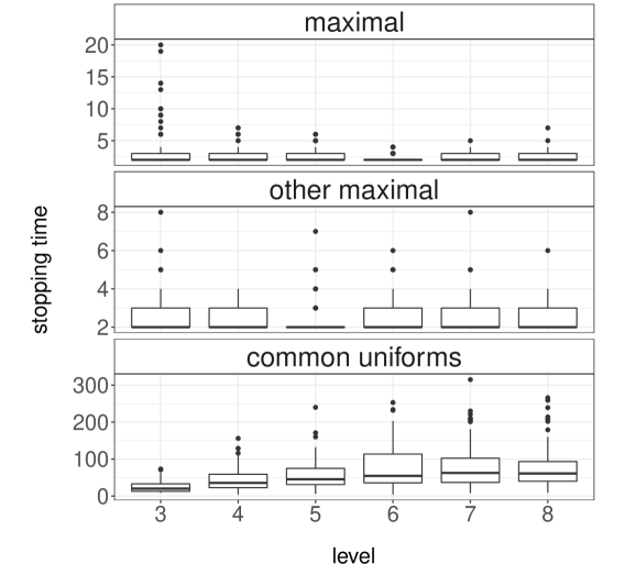
(a) Boxplots of stopping time $\bar{\tau}_{\theta}^{l}$ against discretization level $l$

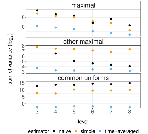
(b) Variance of score increment estimator summed over components $\sum_{j=1}^{d_{\theta}}\mathrm{Var}[\widehat{I}_{l}(\theta)^{j}]$ against discretization level $l$

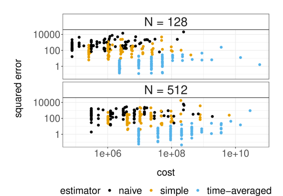
(c) Squared error $\|\widehat{S}(\theta)-S(\theta)\|_{2}^{2}$ against cost with $N\in\{128,512\}$ particles

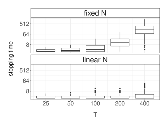
(d) Boxplots of stopping time $\bar{\tau}_{\theta}^{l}$ against number of observations $T$ for discretization level $l=6$ with $N=128$ fixed or linearly increasing number of particles

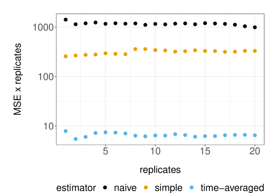
(e) Mean squared error $\mathrm{MSE}(\theta)=\mathbb{E}[\|\bar{S}(\theta)-S(\theta)\|_{2}^{2}]$ against number of averaged replicates $R$

(f) Boxplots of cost against number of averaged replicates $R$

Figure 1: Behaviour of different coupling methods and score estimators at the data generating parameter $\theta=(2,7,1)$ of the Ornstein–Uhlenbeck model in Section 5.1. $T=25$ observations and $N=128$ particles were employed unless stated otherwise. These plots are based on $100$ independent repetitions.

5.2 Logistic diffusion model for population dynamics of red kangaroos

Next we consider an application from population ecology to model the dynamics of a population of red kangaroos (Macropus rufus) in New South Wales, Australia. Figure 2(a) displays data $y_{t_{1}},\ldots,y_{t_{P}}\in\mathbb{N}_{0}^{2}$ from Caughley et al. (1987), which are double transect counts on $P=41$ occasions at irregular times $(t_{p})_{p=1}^{P}$ between $1973$ to $1984$. The latent population size $Z=(Z_{t})_{t_{1}\leq t\leq t_{P}}$ is assumed to follow a logistic diffusion process with environmental variance (Dennis and Costantino, 1988; Knape and De Valpine, 2012)

$$dZ_{t}=(\theta_{3}^{2}/2+\theta_{1}-\theta_{2}Z_{t})Z_{t}dt+\theta_{3}Z_{t}dW_{t},\quad Z_{t_{1}}\sim\mathcal{LN}(5,10^{2}),$$ (33)

where $\mathcal{LN}$ denotes the log-Normal distribution. The parameters $\theta_{1}\in\mathbb{R}$ and $\theta_{2}>0$ can be seen as coefficients describing how the growth rate depends on the population size. As the parameter $\theta_{3}>0$ appears in the diffusion coefficient of (33), we apply the Lamperti transformation $X_{t}=\Psi(Z_{t})=\log(Z_{t})/\theta_{3}$. By Itô’s lemma, the transformed process $X=(X_{t})_{t_{1}\leq t\leq t_{P}}$ satisfies the SDE (1) with random initialization $X_{t_{1}}\sim\mu_{\theta}=\mathcal{N}(5/\theta_{3},10^{2}/\theta_{3}^{2})$, drift function $a_{\theta}(x)=\theta_{1}/\theta_{3}-(\theta_{2}/\theta_{3})\exp(\theta_{3}x)$ and unit diffusion coefficient $\sigma(x)=1$ for $x\in\mathbb{R}$. The observations $(Y_{t_{p}})_{p=1}^{P}$ are modelled as conditionally independent given $X$ and negative Binomial distributed, i.e. the observation density at time $t\in\{t_{1},\ldots,t_{P}\}$ is $g_{\theta}(y_{t}|x_{t})=\mathcal{NB}(y_{t}^{1};\theta_{4},\exp(\theta_{3}x_{t}))\mathcal{NB}(y_{t}^{2};\theta_{4},\exp(\theta_{3}x_{t}))$, where $\theta_{4}>0$. We will use a parameterization of the negative Binomial distribution that is common in ecology, $\mathcal{NB}(y;r,\mu)=\frac{\Gamma(y+r)}{\Gamma(r)y!}(\frac{r}{r+\mu})^{r}(\frac{\mu}{r+\mu})^{y}$ for $y\in\mathbb{N}_{0}$, where $r>0$ is the dispersion parameter and $\mu>0$ is the mean parameter. The $d_{\theta}=4$ unknown parameters to be inferred are $\theta=(\theta_{1},\theta_{2},\theta_{3},\theta_{4})\in\Theta=\mathbb{R}\times(0,\infty)^{3}$.

Application of our methodology requires some minor modifications. As the initial distribution $\mu_{\theta}$ depends on $\theta_{3}$, the representation of score functions in (5) and (12) require adding $\nabla_{\theta}\log\mu_{\theta}(X_{t_{1}})$ to (8) and (2.2); see Appendix B.2 for model-specific expressions. To deal with irregular observation times $(t_{p})_{p=1}^{P}$, we set the step-size at discretization level zero as the size of the smallest time interval, i.e. $\Delta_{0}=\min_{p=2,\ldots,P}t_{p}-t_{p-1}$. Higher levels $l\in\mathbb{N}$ will employ $\Delta_{l}=\Delta_{0}2^{-l}$. For level $l\in\mathbb{N}_{0}$, the first time interval $[t_{1},t_{2}]$ is discretized using $\Delta_{l}$ sequentially, i.e. we set $s_{k}=t_{1}+k\Delta_{l}$ for $k\in\{0,\ldots,m_{l,1}\}$ with $m_{l,1}=\left\lfloor(t_{2}-t_{1})/\Delta_{l}\right\rfloor$, and $s_{k}=t_{2}$ for $k=m_{l,1}+1$ if $(t_{2}-t_{1})/\Delta_{l}\notin\mathbb{N}$. The subsequent time intervals are then discretized in the same manner.

Figure 2(b) illustrates how the median and the 90% quantile of the stopping time $\bar{\tau}_{\theta}^{l}$ vary with the discretization level $l$, the impact of the number of particles $N$ and the benefits of employing adaptive resampling. As before, the coupled resampling scheme in Algorithm 5 results in stopping times that are smaller for higher discretization levels, with less variability over levels as the number of particles increases. Moreover, resampling only when the effective sample size is less than $N/2$ allows us to induce more dependencies between the multiple CPF chains at lower discretization levels. Using $N=256$ particles and adaptive resampling, Figure 2(c) examines the rate at which the variance of the estimated increment decreases with the discretization level. Here we consider the “naive” and “simple” estimators described in Section 5.1, with a burn-in of $b=90\%\textrm{-quantile}(\bar{\tau}_{\theta}^{l})$ at level $l=3$, and omit the more costly “time-averaged” estimator. From the plot, both type of estimators have similar rate of decay and are valid choices in our score estimation methodology. Using the “simple” estimator, Figure 2(d) verifies that the average of $R$ independent replicates of the resulting score estimator $\bar{S}(\theta)$ satisfies the standard Monte Carlo rate as $R\rightarrow\infty$.

Lastly, we perform Bayesian parameter inference by employing our score estimators within the SGLD framework (Welling and Teh, 2011). We rely on logarithmic transformations to deal with positivity parameter constraints, and specify the prior distribution $(\theta_{1},\log\theta_{2},\log\theta_{3},\log\theta_{4})\sim\mathcal{N}_{d_{\theta}}(\mu_{0},\Sigma_{0})$, where $\mu_{0}=(0,-1,-1,-1)$ and $\Sigma_{0}=\textrm{diag}(5^{2},2^{2},2^{2},2^{2})$. As $\log\theta_{3}$ has a significantly different scale compared to the other parameters, we let the learning rate in (4) be component-dependent by taking $\varepsilon_{m}=\textrm{diag}((100+m)^{-0.6}(10^{-2},10^{-2},10^{-4},10^{-2}))$ at iteration $m\geq 1$. The algorithmic settings used to produce score estimators are the same as in Figure 2(d) with $R=1$ realization. Figure 2(e) shows the trace plot over $7500$ iterations of the resulting SGLD algorithm for each parameter.

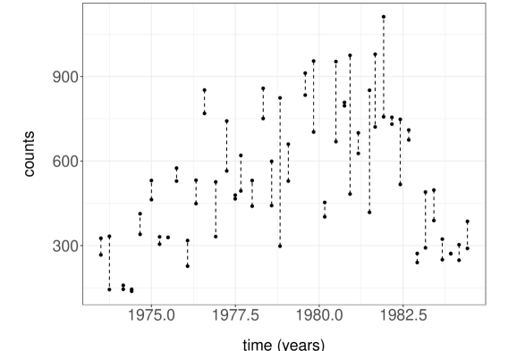
(a) Double transect counts

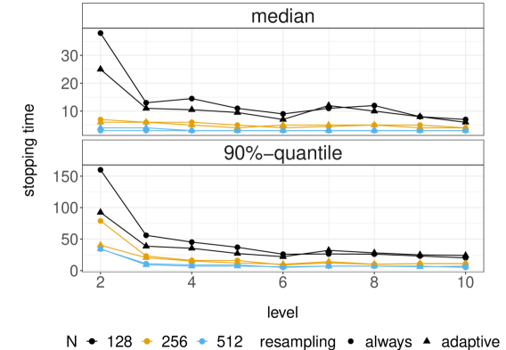
(b) Sample median and 90% quantile of stopping time $\bar{\tau}_{\theta}^{l}$ against discretization level $l$

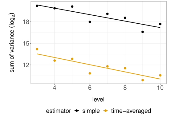
(c) Variance of score increment estimator summed over components $\sum_{j=1}^{d_{\theta}}\mathrm{Var}[\widehat{I}_{l}(\theta)^{j}]$ against discretization level $l$

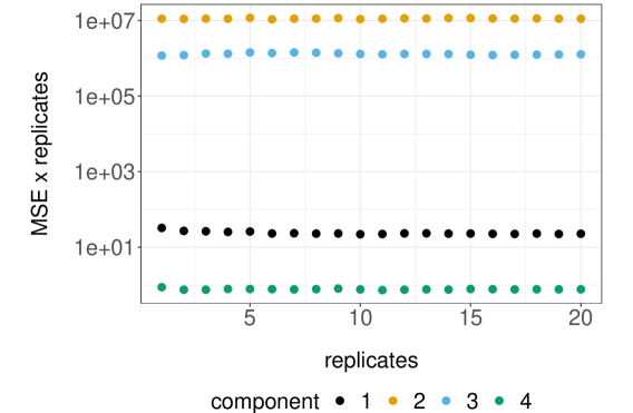
(d) Mean squared error $\mathrm{MSE}(\theta)^{j}=\mathbb{E}[|\bar{S}(\theta)^{j}-S(\theta)^{j}|^{2}]$ against number of averaged replicates $R$ for component $j\in\{1,\ldots,d_{\theta}\}$

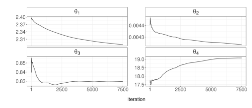
(e) SGLD for each component.

Figure 2: Behaviour at parameter $\theta=(2.397,4.429\times 10^{-3},0.840,17.631)$ of the logistic diffusion model in Section 5.2. $N=256$ particles were employed unless stated otherwise. These plots are based on $100$ independent repetitions.

5.3 Neural network model for grid cells in the medial entorhinal cortex

As our final application, we consider a neural network model for single neurons to analyze grid cells spike data recorded in the medial entorhinal cortex of rats that were running on a linear track (Hafting et al., 2008). The neural states $Z_{t}=(Z_{t}^{1},Z_{t}^{2})$ of two grid cells that were simultaneously recorded is assumed to follow

$$dZ_{t}^{1} =\left(\alpha_{1}\tanh(\beta_{1}Z_{t}^{2}+\gamma_{1})-\delta_{1}Z_{t}^{1}\right)dt+\sigma_{1}dW_{t}^{1},$$ (34)

$$dZ_{t}^{2} =\left(\alpha_{2}\tanh(\beta_{2}Z_{t}^{1}+\gamma_{2})-\delta_{2}Z_{t}^{2}\right)dt+\sigma_{2}dW_{t}^{2},$$

for $t\in[0,T]$, where $(\alpha_{1},\alpha_{2})\in\mathbb{R}^{2}$ controls the amplitude, $(\beta_{1},\beta_{2})\in\mathbb{R}^{2}$ describes the connectivity between the cells, $(\gamma_{1},\gamma_{2})\in\mathbb{R}^{2}$ are baseline levels, $(\delta_{1},\delta_{2})\in(0,\infty)^{2}$ determines the strength of the mean reversion towards the origin. We assume $Z_{0}=(0,0)$ at the beginning of the experiment. This diffusion is motivated by an example in Kappen and Ruiz (2016), and modified for our purposes. To infer the unknown diffusivity parameters $(\sigma_{1},\sigma_{2})\in(0,\infty)^{2}$, we consider the transformation $X_{t}=(X_{t}^{1},X_{t}^{2})=\Psi(Z_{t})=(Z_{t}^{1}/\sigma_{1},Z_{t}^{2}/\sigma_{2})$, which rescales each component of the diffusion. By Itô’s formula, the transformed process $X=(X_{t})_{0\leq t\leq T}$ satisfies the diffusion model (1) with initialization $x_{\star}=(0,0)$, drift function

$$a_{\theta}(x)=\left(\begin{array}[]{c}a_{\theta}^{1}(x)\\ a_{\theta}^{2}(x)\end{array}\right)=\left(\begin{array}[]{c}\alpha_{1}\tanh(\beta_{1}\sigma_{2}x^{2}+\gamma_{1})/\sigma_{1}-\delta_{1}x^{1}\\ \alpha_{2}\tanh(\beta_{2}\sigma_{1}x^{1}+\gamma_{2})/\sigma_{2}-\delta_{2}x^{2}\end{array}\right),$$ (39)

and diffusion coefficient $\sigma(x)=I_{2}$ for $x=(x^{1},x^{2})\in\mathbb{R}^{2}$.

The experimental data over a duration of $T=20$ seconds contains time stamps in $[0,T]$ when a spike at one of the two cells is recorded using tetrodes. Following Brown (2005), we adopt an inhomogenous Poisson point process to model these times. Let $t_{p}=pT2^{-6}$ for $p\in\{0,1,\ldots,P\}$ denote a dyadic uniform discretization of $[0,T]$ into $P=2^{6}$ time intervals. Given the latent process $X=(X_{t})_{0\leq t\leq T}$, the number of spikes $Y_{t_{p}}^{i}$ occurring in each time interval $[t_{p-1},t_{p}]$ at cell $i=1,2$ is assumed to be conditionally independent of the other time intervals and the activity in the other cell, and follow a Poisson distribution with rate $\int_{t_{p-1}}^{t_{p}}\lambda_{i}(X_{t}^{i})dt$. The intensity function for grid cell $i=1,2$ is modelled as $\lambda_{i}(X_{t}^{i})=\exp(\kappa_{i}+X_{t}^{i})$, where $\kappa_{i}\in\mathbb{R}$ represents a baseline level. The observed counts $y_{t_{p}}=(y_{t_{p}}^{1},y_{t_{p}}^{2})$ for interval $p\in\{1,\ldots,P\}$, computed from the experimental data, are displayed in Figure 3(a). The conditional likelihood of the observation model is $p_{\theta}(y_{t_{1}},\ldots,y_{t_{P}}|X)=\prod_{p=1}^{P}g_{\theta}(y_{t_{p}}|(X_{t})_{t_{p-1}\leq t\leq t_{p}})$ with the intractable observation density

$$g_{\theta}(y_{t_{p}}|(X_{t})_{t_{p-1}\leq t\leq t_{p}})=\prod_{i=1}^{2}\mathcal{P}oi\left(y_{t_{p}}^{i};\int_{t_{p-1}}^{t_{p}}\lambda_{i}(X^{i}_{t})dt\right),$$ (40)

where $\mathcal{P}oi(y;\lambda)=\lambda^{y}\exp(-\lambda)/y!$ for $y\in\mathbb{N}_{0}$ denotes the PMF of a Poisson distribution with rate $\lambda>0$. To approximate the conditional likelihood, at level $l\geq 6$, we discretize the time interval $[0,T]$ in a similar manner using $s_{k}=k\Delta_{l}$ for $k\in\{0,1,\ldots,K_{l}\}$, where $\Delta_{l}=T2^{-l}$ is the step-size and $K_{l}=2^{l}$ is the number of time steps. Under the time-discretized process $X_{0:T}=(X_{s_{k}})_{k=0}^{K_{l}}$, the resulting approximation of the conditional likelihood is $p^{l}_{\theta}(y_{t_{1}},\ldots,y_{t_{P}}|X_{0:T})=\prod_{p=1}^{P}g^{l}_{\theta}(y_{t_{p}}|(X_{t})_{t_{p-1}\leq t\leq t_{p}})$ with the corresponding observation density

$$g^{l}_{\theta}(y_{t_{p}}|(X_{t})_{t_{p-1}\leq t\leq t_{p}})=\prod_{i=1}^{2}\mathcal{P}oi\left(y_{t_{p}}^{i};\Delta_{l}\sum_{t:t_{p-1}\leq t\leq t_{p}}\lambda_{i}(X^{i}_{t})\right).$$ (41)

By using these level-dependent observation densities (41) in Section 2.2, our proposed methodology can then be applied. There are $d_{\theta}=12$ parameters $\theta=(\theta_{1},\theta_{2})$ to be inferred, where $\theta_{i}=(\alpha_{i},\beta_{i},\gamma_{i},\delta_{i},\sigma_{i},\kappa_{i})$ denote the parameters associated to cell $i=1,2$. We refer the reader to Appendix B.3 for model-specific expressions to evaluate (2.2).

We consider an extension of the proposed method based on the conditional ancestor sampling particle filter (CASPF) (Lindsten et al., 2014) as the basic algorithmic building block. As CASPF has better mixing properties than CPF, we observe smaller stopping times in Figure 3(b) for lower discretization levels. Figure 3(c) verifies the validity of using both MCMC algorithms and “naive” and “simple” estimators (as described in Section 5.1) within our methodology. For “simple” estimators, the burn-in was taken as $b=90\%\textrm{-quantile}(\bar{\tau}_{\theta}^{l})$ at level $l=11$. The rate at which the variance of the estimated increment decays with the discretization level is similar across algorithms and estimators.

Lastly, we combine our score estimators and the SGA scheme in (3) to perform maximum likelihood estimation. The score estimation relies on the CASPF algorithm and the “simple” estimator with a burn-in of $b=100$. Positivity parameter constraints are dealt with using logarithmic transformations and a constant learning rate of $\varepsilon_{m}=10^{-3}$ is employed. Figure 3(d) illustrates how the distribution of the Polyak–Ruppert average evolves over the iterations, estimated using independent runs of SGA. We note that only $87$ out of $100$ runs were considered, as there were $13$ instances of the variance of the score estimator driving the SGA algorithm to regions of the parameter space where the stopping times are prohibitively large, causing the SGA to stall. This pathological behaviour is due to poor mixing properties of the underlying CASPF algorithm at very unlikely regions of the parameter space. To improve the MCMC algorithm, one has to simulate particle dynamics that incorporate information from the observation sequence $y_{t_{1}},\ldots,y_{t_{P}}$, which could be investigated in future work. The parameter estimates of $\beta_{1}$ and $\beta_{2}$ support the use of a joint model (34) for both grid cells, and indicates that these cells are positively dependent.

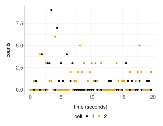
(a) Counts $y_{t_{p}}=(y_{t_{p}}^{1},y_{t_{p}}^{2})$ on time intervals of duration $T2^{-6}=0.3125$ second

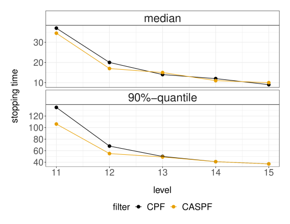
(b) Sample median and 90% quantile of stopping time $\bar{\tau}_{\theta}^{l}$ against discretization level $l$

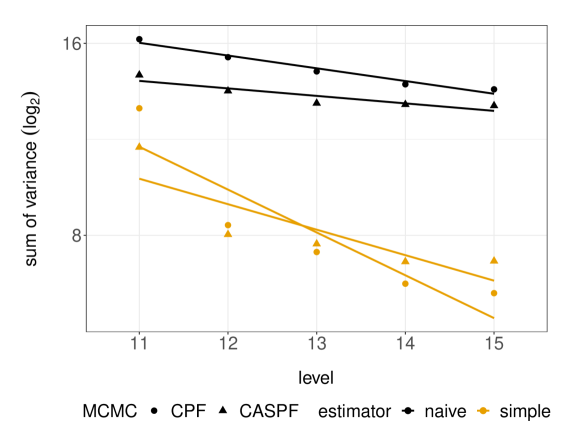
(c) Variance of score increment estimator summed over components $\sum_{j=1}^{d_{\theta}}\mathrm{Var}[\widehat{I}_{l}(\theta)^{j}]$ against discretization level $l$

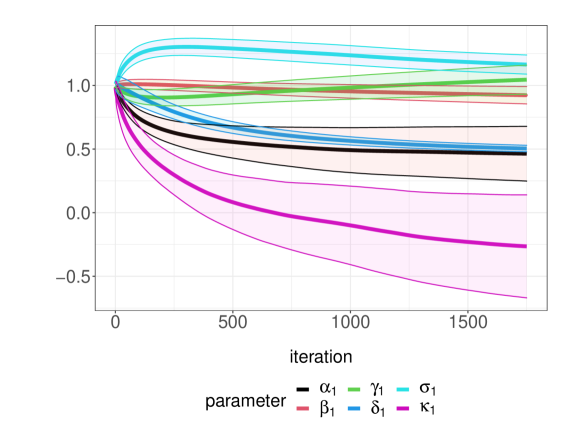
(d) Mean ($\pm$ one standard deviation) of Polyak–Ruppert average for parameter estimates of $\theta_{1}$ over $87$ runs of SGA

Figure 3: Behaviour at parameter $\theta=(1,\dots,1)$ of the neural network model in Section 5.3. The algorithmic settings involve $N=256$ particles and adaptive resampling. These plots are based on $1000$ independent repetitions unless stated otherwise.

6 Parameter dependence in diffusion coefficient

We end this article by considering how one can extend the ideas in this article to accommodate the case where the diffusion coefficient also depends on the parameter $\theta\in\Theta$. In this case, we have the SDE

$$dX_{t}=a_{\theta}(X_{t})dt+\sigma_{\theta}(X_{t})dW_{t},\quad X_{0}=x_{\star}\in\mathbb{R}^{d},$$ (42)

where $\sigma:\Theta\times\mathbb{R}^{d}\rightarrow\mathbb{R}^{d\times d}$ is assumed to be such that $\theta\mapsto\sigma_{\theta}$ is invertible and satisfies the conditions in Assumption 1 uniformly in $\theta\in\Theta$. Moreover, we shall suppose that all the conditions in Schauer et al. (2017) hold. For $k\in\mathbb{N}_{0}$ and $t\in[k,k+1]$, consider the diffusion bridge

$$dX_{t}=a_{\theta}^{\circ}(X_{t})dt+\sigma_{\theta}(X_{t})dW_{t},\quad X_{k}=x_{k},\leavevmode\nobreak\ X_{k+1}=x_{k+1},$$ (43)

where the drift function $a_{\theta}^{\circ}$ is described in Schauer et al. (2017). Given a Brownian path $\bm{W}_{k}=(W_{t})_{k\leq t\leq k+1}$, we denote the path-wise solution of the diffusion bridge as $F_{\theta,k}(\bm{W}_{k},x_{k},x_{k+1})$. Furthermore, for $G:\Theta\times\mathbb{R}^{d}\rightarrow\mathbb{R}$ given in Schauer et al. (2017, Equation 2.3) and a process $\bm{Z}_{k}=(Z_{t})_{k\leq t\leq k+1}$, we define the functional

$$H_{\theta,k}(\bm{Z}_{k})=\int_{k}^{k+1}G_{\theta}(Z_{t})dt.$$ (44)

Using the change of measure in Schauer et al. (2017) along with the approach in Beskos et al. (2021) and Yonekura and Beskos (2020), one can write the marginal likelihood of observations $y_{1:T}=(y_{t})_{t=1}^{T}$ as

$$p_{\theta}(y_{1:T})=\widetilde{\mathbb{E}}_{\theta}\left[\prod_{t=1}^{T}g_{\theta}(y_{t}|X_{t})\exp\Big{\{}\sum_{t=0}^{T-1}H_{\theta,t}(F_{\theta,t}(\bm{W}_{t},X_{t},X_{t+1}))\Big{\}}\right].$$ (45)

In the above, $\widetilde{\mathbb{E}}_{\theta}$ denotes expectation w.r.t. the probability measure $\widetilde{\mathbb{P}}_{\theta}$ defined as

$$\widetilde{\mathbb{P}}_{\theta}(d(x_{1},\dots,x_{T},\bm{W}_{0},\dots,\bm{W}_{T-1}))=\prod_{t=1}^{T}\bigg{\{}\widetilde{p}_{\theta}(x_{t-1},x_{t})dx_{t}\bigg{\}}\widetilde{\mathbb{W}}(d(\bm{W}_{0},\dots,\bm{W}_{T-1})),$$ (46)

where $\widetilde{p}_{\theta}(x_{t-1},x_{t})$ is the transition density of an auxiliary process on a unit time interval as constructed in Schauer et al. (2017) that is known and can be sampled, and $\widetilde{\mathbb{W}}(d(\bm{W}_{0},\dots,\bm{W}_{T-1}))=\bigotimes_{k=0}^{T-1}\mathbb{W}(d\bm{W}_{k})$ is given by the Wiener measure $\mathbb{W}$.

Under regularity conditions, one can differentiate (45) and represent the score function as

$$S(\theta)=\breve{\mathbb{E}}_{\theta}\left[\sum_{t=1}^{T}\nabla_{\theta}\log g_{\theta}(y_{t}|X_{t})+\sum_{t=1}^{T}\nabla_{\theta}\log\widetilde{p}_{\theta}(X_{t-1},X_{t})+\sum_{t=1}^{T-1}\nabla_{\theta}H_{\theta,t}(F_{\theta,t}(\mathbf{W}_{t},X_{t},X_{t+1}))\right],$$ (47)

where $\breve{\mathbb{E}}_{\theta}$ denotes expectation w.r.t. the probability measure

$$\breve{\mathbb{P}}_{\theta}(d(x_{1},\dots,x_{T},\bm{W}_{0},\dots,\bm{W}_{T-1}))$$

$$=\leavevmode\nobreak\ p_{\theta}(y_{1:T})^{-1}\prod_{t=1}^{T}g_{\theta}(y_{t}|x_{t})\exp\Big{\{}\sum_{t=0}^{T-1}H_{\theta,t}(F_{\theta,t}(\mathbf{W}_{t},x_{t},x_{t+1}))\Big{\}}\widetilde{\mathbb{P}}_{\theta}(d(x_{1},\dots,x_{T},\bm{W}_{0},\dots,\bm{W}_{T-1})).$$ (48)

Practical implementation will require a discretized approximation of $\nabla_{\theta}H_{\theta,p}(F_{\theta,p}(\cdot))$, which involves a gradient w.r.t. $\theta$ of a path-wise solution of the diffusion bridge (43). Although Euler-type approximations can be obtained, the resulting bias in the sense of Theorem 1 is significantly more complicated to analyze and is thus left as future work. We stress that only small modifications to our proposed methodology is necessary to obtain unbiased estimators of the score function in this case. A similar approach is considered in Beskos et al. (2021) for a class of continuous-time models. Alternatively, one could also consider using Malliavan techniques (see e.g. Fournié et al. (1999)), instead of the ideas described here.

Acknowledgements

Ajay Jasra was supported by KAUST baseline funding. Jeremy Heng was funded by CY Initiative of Excellence (grant “Investissements d’Avenir” ANR-16-IDEX-0008).

Appendix A Theoretical analysis

A.1 Introduction and preliminaries

Section A.2 provides some results on time-discretization of diffusions, which are needed for the proofs associated to Theorem 1 as well as the 4-CCPF (Algorithm 4). Our main technical arguments associated to Theorem 2 are given in Section A.3, followed by several remarks about the proofs and discussions of alternative strategies. This section of the appendix is intended to be read in the order in which it is presented. Some familiarity with the approach in Jasra et al. [2017] is also useful.

Note that our results concerning $\mathbb{L}_{r}$-norms are stated for $r\in[1,\infty)$; and can be extended to the case $r\in(0,1)$ by Hölder’s inequality. We will use this fact without further elaboration. Throughout our arguments, $C$ will represent a finite constant whose value may change from line to line, but does not depend upon the discretization level. Any other dependencies in the various parameters considered will be made explicit in the statement of our results.

A.2 Results on time-discretized diffusion processes

In this section, we consider two diffusion process $X=(X_{t})_{t\geq 0}$ and $X^{\star}=(X_{t}^{\star})_{t\geq 0}$ on the filtered probability space $(\Omega,\mathscr{F},\{\mathscr{F}_{t}\}_{t\geq 0},\mathbb{P}_{\theta})$ following (1), with the respective initial conditions $X_{0}=x\in\mathbb{R}^{d}$ and $X_{0}^{\star}=x_{\star}\in\mathbb{R}^{d}$, and driven by the same Brownian motion. We will consider Euler discretizations (10) of $(X_{t})_{t\geq 0}$ and $(X_{t}^{\star})_{t\geq 0}$ at some given level $l$, denoted as $\widetilde{X}_{0:T}$ and $\widetilde{X}_{0:T}^{\star}$, driven by the same Brownian motion and with the initial conditions $\widetilde{X}_{0}=x$ and $\widetilde{X}_{0}^{\star}=x_{\star}$. The expectation operator for the described processes is written as $\mathbb{E}_{\theta}$. Although many proof strategies in this section follow Crisan [2011], we note that many of these arguments will be used in Section A.3 to study coupled CPFs.

In addition to the previously defined terms $b_{\theta}(x)=\Sigma(x)^{-1}\sigma(x)^{*}a_{\theta}(x)$ and $\Sigma(x)=\sigma(x)\sigma(x)^{*}$, we introduce the function $\rho_{\theta}(x)=b_{\theta}(x)^{*}\Sigma(x)^{-1}\sigma(x)^{*}$ which allows us to rewrite (8) and (2.2) as

$$G_{\theta}(X) =-\frac{1}{2}\int_{0}^{T}\nabla_{\theta}\|b_{\theta}(X_{t})\|_{2}^{2}dt+\int_{0}^{T}\nabla_{\theta}\rho_{\theta}(X_{t})dX_{t}+\sum_{t=1}^{T}\nabla_{\theta}\log g_{\theta}(y_{t}|X_{t}),$$ (49)

$$G_{\theta}^{l}(X_{0:T})= -\frac{1}{2}\sum_{k=1}^{K_{l}}\nabla_{\theta}\|b_{\theta}(X_{s_{k-1}})\|_{2}^{2}\Delta_{l}+\sum_{k=1}^{K_{l}}\nabla_{\theta}\rho_{\theta}(X_{s_{k-1}})(X_{s_{k}}-X_{s_{k-1}})+\sum_{t=1}^{T}\nabla_{\theta}\log g_{\theta}(y_{t}|X_{t}).$$ (50)

For notational convenience, we define the $d\times 1$ vector of derivatives of $\rho_{\theta}$ as

$$\kappa_{\theta,i}(x)^{*}=\Big{(}\frac{\partial}{\partial\theta_{i}}[\rho_{\theta}(x)]^{1},\dots,\frac{\partial}{\partial\theta_{i}}[\rho_{\theta}(x)]^{d}\Big{)},$$

for any $(i,x)\in\{1,\dots,d_{\theta}\}\times\mathbb{R}^{d}$, and the conditional likelihood given states $x_{1},\dots,x_{T}\in\mathbb{R}^{d}$ as $\varphi_{\theta}(x_{1},\dots,x_{T})=\prod_{t=1}^{T}g_{\theta}(y_{t}|x_{t})$. We now give the proof of Theorem 1 followed by several technical lemmata that are required to establish the theorem.

Proof of Theorem 1.

We consider the proof for any given component $i\in\{1,\dots,d_{\theta}\}$ and decompose the error of the score function (12) at level $l\in\mathbb{N}_{0}$ as

$$[S_{l}(\theta)-S(\theta)]^{i}=T_{1}+T_{2}$$ (51)

where

$$T_{1} =\frac{\mathbb{E}_{\theta}[\varphi_{\theta}(\widetilde{X}_{1}^{\star},\dots,\widetilde{X}_{T}^{\star})[G_{\theta}^{l}(\widetilde{X}_{0:T}^{\star})]^{i}]}{\mathbb{E}_{\theta}[\varphi_{\theta}(\widetilde{X}_{1}^{\star},\dots,\widetilde{X}_{T}^{\star})]\mathbb{E}_{\theta}[\varphi_{\theta}(X_{1}^{\star},\dots,X_{T}^{\star})]}\Big{(}\mathbb{E}_{\theta}[\varphi_{\theta}(X_{1}^{\star},\dots,X_{T}^{\star})]-\mathbb{E}_{\theta}[\varphi_{\theta}(\widetilde{X}_{1}^{\star},\dots,\widetilde{X}_{T}^{\star})]\Big{)},$$

$$T_{2} =\frac{1}{\mathbb{E}_{\theta}[\varphi_{\theta}(X_{1}^{\star},\dots,X_{T}^{\star})]}\Big{(}\mathbb{E}_{\theta}[\varphi_{\theta}(\widetilde{X}_{1}^{\star},\dots,\widetilde{X}_{T}^{\star})[G_{\theta}^{l}(\widetilde{X}_{0:T}^{\star})]^{i}]-\mathbb{E}_{\theta}[\varphi_{\theta}(X_{1}^{\star},\dots,X_{T}^{\star})[G_{\theta}(X^{\star})]^{i}]\Big{)}.$$

Thus our objective is to provide bounds on the quantities $T_{1}$ and $T_{2}$ to conclude the proof.

For $T_{1}$, using Assumption 2, one has the upper-bound

$$T_{1}\leq C\sum_{t=1}^{T}\mathbb{E}_{\theta}[\|\widetilde{X}_{t}^{\star}-X_{t}^{\star}\|_{2}],$$

then by using results on the convergence of Euler approximations (e.g. Kloeden and Platen [2013]), for $r>0$

$$\mathbb{E}_{\theta}\big{[}\|\widetilde{X}^{\star}_{t}-X^{\star}_{t}\|_{2}^{r}\big{]}^{1/r}\leq C\Delta_{l}^{1/2}$$ (52)

one has

$$T_{1}\leq C\Delta_{l}^{1/2}.$$ (53)

Note that using standard results on weak errors for diffusions one can improve this upper-bound to $T_{1}\leq C\Delta_{l}$.

For $T_{2}$, using Assumption 2, we have $T_{2}\leq C(T_{3}+T_{4})$ where

$$T_{3} =\mathbb{E}_{\theta}\big{[}\{\varphi_{\theta}(\widetilde{X}_{1}^{\star},\dots,\widetilde{X}_{T}^{\star})-\varphi_{\theta}(X_{1}^{\star},\dots,X_{T}^{\star})\}[G_{\theta}^{l}(\widetilde{X}_{0:T}^{\star})]^{i}\big{]},$$

$$T_{4} =\mathbb{E}_{\theta}\big{[}\varphi_{\theta}(X_{1}^{\star},\dots,X_{T}^{\star})\{[G_{\theta}^{l}(\widetilde{X}_{0:T}^{\star})]^{i}-[G_{\theta}(X^{\star})]^{i}\}\big{]}.$$

For $T_{3}$, using Cauchy-Schwarz, we have the upper-bound

$$T_{3}\leq\mathbb{E}_{\theta}\big{[}\{\varphi_{\theta}(\widetilde{X}_{1}^{\star},\dots,\widetilde{X}_{T}^{\star})-\varphi_{\theta}(X_{1}^{\star},\dots,X_{T}^{\star})\}^{2}\big{]}^{1/2}\mathbb{E}_{\theta}\big{[}\{[G_{\theta}^{l}(\widetilde{X}_{0:T}^{\star})]^{i}\}^{2}\big{]}^{1/2}.$$

As the second term is bounded by $C$, we consider only the first. We have the upper-bound

$$T_{3}\leq C\sum_{t=1}^{T}\mathbb{E}_{\theta}\big{[}\|\widetilde{X}_{t}^{\star}-X_{t}^{\star}\|_{2}^{2}\big{]}^{1/2}\leq C\Delta_{l}^{1/2}.$$ (54)

For $T_{4}$, noting that $\varphi_{\theta}$ is a bounded function under Assumption 2, applying Lemma 1 allows one to conclude that $T_{4}\leq C\Delta_{l}^{1/2}$. Therefore, using $T_{2}\leq C(T_{3}+T_{4})$ along with (54), we have

$$T_{2}\leq C\Delta_{l}^{1/2}.$$ (55)

Combining (53) and (55) with (51) allows one to conclude the proof. ∎

Lemma 1.

Under Assumptions 1 and 2, for any $(T,r,\theta,i)\in\mathbb{N}\times[1,\infty)\times\Theta\times\{1,\dots,d_{\theta}\}$, there exists a constant $C<\infty$ such that for any $(l,x)\in\mathbb{N}_{0}\times\mathbb{R}^{d}$

$$\mathbb{E}_{\theta}\Big{[}\big{|}[G_{\theta}^{l}(\widetilde{X}_{0:T})]^{i}-[G_{\theta}(X)]^{i}\big{|}^{r}\Big{]}^{1/r}\leq C\Delta_{l}^{1/2},$$

with $\widetilde{X}_{0}=X_{0}=x$.

Proof.

We have that

$$\mathbb{E}_{\theta}\Big{[}\big{|}[G_{\theta}^{l}(\widetilde{X}_{0:T})]^{i}-[G_{\theta}(X)]^{i}\big{|}^{r}\Big{]}\leq C(T_{1}+T_{2})$$ (56)

where

$$T_{1} =\mathbb{E}_{\theta}\Big{[}\big{|}[G_{\theta}^{l}(\widetilde{X}_{0:T})]^{i}-[G^{l}_{\theta}(X_{0:T})]^{i}\big{|}^{r}\Big{]},$$

$$T_{2} =\mathbb{E}_{\theta}\Big{[}\big{|}[G_{\theta}^{l}(X_{0:T})]^{i}-[G_{\theta}(X)]^{i}\big{|}^{r}\Big{]},$$

where $X_{0:T}=(X_{s_{k}})_{k=0}^{K_{l}}$ are the states of the process $(X_{t})_{t\geq 0}$ at the discretization times of the process $\widetilde{X}_{0:T}$. From (50), we have that $T_{1}\leq C\sum_{j=3}^{6}T_{j}$, where

$$T_{3} =\mathbb{E}_{\theta}\Big{[}\Big{|}\sum_{t=1}^{T}\Big{\{}\big{[}\nabla_{\theta}\log g_{\theta}(y_{t}|\widetilde{X}_{t})\big{]}^{i}-\big{[}\nabla_{\theta}\log g_{\theta}(y_{t}|X_{t})\big{]}^{i}\Big{\}}\Big{|}^{r}\Big{]},$$

$$T_{4} =\Delta_{l}^{r}\mathbb{E}_{\theta}\Big{[}\Big{|}\sum_{k=1}^{K_{l}}\Big{\{}\big{[}\nabla_{\theta}\|b_{\theta}(\widetilde{X}_{s_{k-1}})\|_{2}^{2}\big{]}^{i}-\big{[}\nabla_{\theta}\|b_{\theta}(X_{s_{k-1}})\|_{2}^{2}\big{]}^{i}\Big{\}}\Big{|}^{r}\Big{]},$$

$$T_{5} =\mathbb{E}_{\theta}\Big{[}\Big{|}\sum_{k=1}^{K_{l}}\{\kappa_{\theta,i}(\widetilde{X}_{s_{k-1}})^{*}-\kappa_{\theta,i}(X_{s_{k-1}})^{*}\}[\widetilde{X}_{s_{k}}-\widetilde{X}_{s_{k-1}}]\Big{|}^{r}\Big{]},$$

$$T_{6} =\mathbb{E}_{\theta}\Big{[}\Big{|}\sum_{k=1}^{K_{l}}\kappa_{\theta,i}(X_{s_{k-1}})^{*}[(\widetilde{X}_{s_{k}}-\widetilde{X}_{s_{k-1}})-(X_{s_{k}}-X_{s_{k-1}})]\Big{|}^{r}\Big{]}.$$

The term $T_{3}$ can be treated in almost the same manner as $T_{1}$ in the proof of Theorem 1, i.e. using a similar argument to the proof of the bound on $T_{1}$ in Theorem 1, one can deduce that

$$T_{3}\leq C\Delta_{l}^{r/2}.$$ (57)

For $T_{4}$, using the fact that $\partial/\partial\theta_{i}[b_{\theta}^{2}]^{j}\in\textrm{Lip}_{\|\cdot\|_{2}}(\mathbb{R}^{d})$ for any $(i,j)\in\{1,\dots,d_{\theta}\}\times\{1,\dots,d\}$, we have by first applying Minkowski’s inequality

$$T_{4}\leq C\Delta_{l}^{r}\Big{(}\sum_{k=1}^{K_{l}}\mathbb{E}_{\theta}\big{[}\|\widetilde{X}_{s_{k-1}}-X_{s_{k-1}}\|_{2}^{r}\big{]}^{1/r}\Big{)}^{r}.$$

Then using (52), it follows that

$$T_{4}\leq C\Delta_{l}^{r/2}.$$ (58)

The terms $T_{5}$ and $T_{6}$ are bounded in Lemmata 2-3, so combining (57), (58) and the afore-mentioned lemmata with $T_{1}\leq C\sum_{j=3}^{6}T_{j}$ yields

$$T_{1}\leq C\Delta_{l}^{r/2}.$$

By Lemma 4, $T_{2}\leq C\Delta_{l}^{r/2}$ and thus by (56) the proof is concluded. ∎

Corollary 1.

Under Assumptions 1 and 2, for any $(T,r,\theta)\in\mathbb{N}\times[1,\infty)\times\Theta$, there exists a constant $C<\infty$ such that for any $(l,x)\in\mathbb{N}_{0}\times\mathbb{R}^{d}$

$$\mathbb{E}_{\theta}\Big{[}\big{\|}G_{\theta}^{l}(\widetilde{X}_{0:T})-G_{\theta}(X)\big{\|}_{2}^{r}\Big{]}^{1/r}\leq C\Delta_{l}^{1/2}.$$

Proof.

By Minkowski’s inequality

$$\mathbb{E}_{\theta}\Big{[}\big{\|}G_{\theta}^{l}(\widetilde{X}_{0:T})-G_{\theta}(X)\big{\|}_{2}^{r}\Big{]}^{1/r}\leq\bigg{(}\sum_{i=1}^{d_{\theta}}\mathbb{E}_{\theta}\Big{[}\big{|}[G_{\theta}^{l}(\widetilde{X}_{0:T})]^{i}-[G_{\theta}(X)]^{i}\big{|}^{r}\Big{]}^{2/r}\bigg{)}^{1/2}$$

so the proof follows by Lemma 1. ∎

Lemma 2.

Under Assumptions 1 and 2, for any $(T,r,\theta,i)\in\mathbb{N}\times[1,\infty)\times\Theta\times\{1,\dots,d_{\theta}\}$, there exists a constant $C<\infty$ such that for any $(l,x)\in\mathbb{N}_{0}\times\mathbb{R}^{d}$

$$\mathbb{E}_{\theta}\bigg{[}\Big{|}\sum_{k=1}^{K_{l}}\{\kappa_{\theta,i}(\widetilde{X}_{s_{k-1}})^{*}-\kappa_{\theta,i}(X_{s_{k-1}})^{*}\}[\widetilde{X}_{s_{k}}-\widetilde{X}_{s_{k-1}}]\Big{|}^{r}\bigg{]}\leq C\Delta_{l}^{r/2},$$

with $\widetilde{X}_{0}=X_{0}=x$.

Proof.

We have the decomposition

$$\sum_{k=1}^{K_{l}}\{\kappa_{\theta,i}(\widetilde{X}_{s_{k-1}})^{*}-\kappa_{\theta,i}(X_{s_{k-1}})^{*}\}[\widetilde{X}_{s_{k}}-\widetilde{X}_{s_{k-1}}]=M_{K_{l}}+R_{K_{l}},$$

where

$$M_{K_{l}} =\sum_{k=1}^{K_{l}}\{\kappa_{\theta,i}(\widetilde{X}_{s_{k-1}})^{*}-\kappa_{\theta,i}(X_{s_{k-1}})^{*}\}\sigma(\widetilde{X}_{s_{k-1}})[W_{s_{k}}-W_{s_{k-1}}],$$

$$R_{K_{l}} =\Delta_{l}\sum_{k=1}^{K_{l}}\{\kappa_{\theta,i}(\widetilde{X}_{s_{k-1}})^{*}-\kappa_{\theta,i}(X_{s_{k-1}})^{*}\}a_{\theta}(\widetilde{X}_{s_{k-1}}).$$

Thus by the $C_{r}-$inequality,

$$\mathbb{E}_{\theta}\bigg{[}\Big{|}\sum_{k=1}^{K_{l}}\{\kappa_{\theta,i}(\widetilde{X}_{s_{k-1}})^{*}-\kappa_{\theta,i}(X_{s_{k-1}})^{*}\}[\widetilde{X}_{s_{k}}-\widetilde{X}_{s_{k-1}}]\Big{|}^{r}\bigg{]}\leq C\big{(}\mathbb{E}_{\theta}[|M_{K_{l}}|^{r}]+\mathbb{E}_{\theta}[|R_{K_{l}}|^{r}]\big{)}.$$ (59)

We will bound the two terms on the R.H.S. of (59) individually.

Bound for $\mathbb{E}_{\theta}[|M_{K_{l}}|^{r}]$.

If we define $M_{u}=\sum_{k=0}^{u-1}\{\kappa_{\theta,i}(\widetilde{X}_{s_{k-1}})^{*}-\kappa_{\theta,i}(X_{s_{k-1}})^{*}\}\sigma(\widetilde{X}_{s_{k-1}})[W_{s_{k}}-W_{s_{k-1}}]$ for any $u\in\mathbb{N}_{0}$, then $(M_{u},\mathscr{F}_{u\Delta_{l}})_{u\in\mathbb{N}_{0}}$ is a martingale. It follows from this fact and from an application of the Burkholder-Gundy-Davis (BGD) inequality that

$$\mathbb{E}_{\theta}[|M_{K_{l}}|^{r}]\leq C\mathbb{E}_{\theta}\bigg{[}\Big{|}\sum_{k=1}^{K_{l}}(\{\kappa_{\theta,i}(\widetilde{X}_{s_{k-1}})^{*}-\kappa_{\theta,i}(X_{s_{k-1}})^{*}\}\sigma(\widetilde{X}_{s_{k-1}})[W_{s_{k}}-W_{s_{k-1}}])^{2}\Big{|}^{r/2}\bigg{]},$$

from which Minkowski’s inequality yields

$$\mathbb{E}_{\theta}[|M_{K_{l}}|^{r}]\leq C\bigg{(}\sum_{k=1}^{K_{l}}\mathbb{E}_{\theta}\Big{[}\big{|}\{\kappa_{\theta,i}(\widetilde{X}_{s_{k-1}})^{*}-\kappa_{\theta,i}(X_{s_{k-1}})^{*}\}\sigma(\widetilde{X}_{s_{k-1}})[W_{s_{k}}-W_{s_{k-1}}]\big{|}^{r}\Big{]}^{2/r}\bigg{)}^{r/2}.$$

Using the $C_{r}-$inequality $d^{2}$ times, we obtain the bound

$$\mathbb{E}_{\theta}[|M_{K_{l}}|^{r}]\leq\\ C\Bigg{(}\sum_{k=1}^{K_{l}}\bigg{(}\sum_{(m,j)\in\{1,\dots,d\}^{2}}\mathbb{E}_{\theta}\Big{[}\big{|}\{\kappa_{\theta,i}(\widetilde{X}_{s_{k-1}})-\kappa_{\theta,i}(X_{s_{k-1}})\}^{m}\sigma(\widetilde{X}_{s_{k-1}})^{m,j}[W_{s_{k}}-W_{s_{k-1}}]^{j}\big{|}^{r}\Big{]}\bigg{)}^{2/r}\Bigg{)}^{r/2}.$$

Using the fact that $\sigma^{m,j}\in\mathcal{B}_{b}(\mathbb{R}^{d})$ along with the Cauchy-Schwarz inequality yields

$$\mathbb{E}_{\theta}[|M_{K_{l}}|^{r}]\leq\\ C\Bigg{(}\sum_{k=1}^{K_{l}}\bigg{(}\sum_{(m,j)\in\{1,\dots,d\}^{2}}\mathbb{E}_{\theta}\Big{[}\big{|}\{\kappa_{\theta,i}(\widetilde{X}_{s_{k-1}})-\kappa_{\theta,i}(X_{s_{k-1}})\}^{m}\big{|}^{2r}\Big{]}^{1/2}\mathbb{E}_{\theta}\Big{[}\big{|}[W_{s_{k}}-W_{s_{k-1}}]^{j}\big{|}^{2r}\Big{]}^{1/2}\bigg{)}^{2/r}\Bigg{)}^{r/2}.$$ (60)

Since it holds that $[\kappa_{\theta,i}]^{m}\in\textrm{Lip}_{\|\cdot\|}(\mathbb{R}^{d})$, it follows from the same type of inequality as (52) that

$$\mathbb{E}_{\theta}\Big{[}\big{|}\{\kappa_{\theta,i}(\widetilde{X}_{s_{k-1}})-\kappa_{\theta,i}(X_{s_{k-1}})\}^{m}\big{|}^{2r}\Big{]}^{1/2}\leq C\Delta_{l}^{r/2},$$ (61)

and by standard properties of Brownian motion, we obtain

$$\mathbb{E}_{\theta}\Big{[}\big{|}[W_{s_{k}}-W_{s_{k-1}}]^{j}\big{|}^{2r}\Big{]}^{1/2}\leq C\Delta_{l}^{r/2}.$$ (62)

Combining (60) with (61) and (62) yields the upper-bound

$$\mathbb{E}_{\theta}[|M_{K_{l}}|^{r}]\leq C\Delta_{l}^{r/2}.$$ (63)

Bound for $\mathbb{E}_{\theta}[|R_{K_{l}}|^{r}]$.

We have the upper-bound by Minkowski’s inequality

$$\mathbb{E}_{\theta}[|R_{K_{l}}|^{r}]\leq\Delta_{l}^{r}\bigg{(}\sum_{k=1}^{K_{l}}\mathbb{E}_{\theta}\Big{[}\big{|}\{\kappa_{\theta,i}(\widetilde{X}_{s_{k-1}})^{*}-\kappa_{\theta,i}(X_{s_{k-1}})^{*}\}a_{\theta}(\widetilde{X}_{s_{k-1}})\big{|}^{r}\Big{]}^{1/r}\bigg{)}^{r}.$$

Then applying the $C_{r}-$inequality $d$ times and using the assumption that $a_{\theta}^{j}\in\mathcal{B}_{b}(\mathbb{R}^{d})$ we have the upper-bound

$$\mathbb{E}_{\theta}[|R_{K_{l}}|^{r}]\leq C\Delta_{l}^{r}\bigg{(}\sum_{k=1}^{K_{l}}\sum_{j=1}^{d}\mathbb{E}_{\theta}\Big{[}\big{|}\{\kappa_{\theta,i}(\widetilde{X}_{s_{k-1}})-\kappa_{\theta,i}(X_{s_{k-1}})\}^{j}\big{|}^{r}\Big{]}^{1/r}\bigg{)}^{r}.$$

Using the same argument to obtain (61), we have

$$\mathbb{E}_{\theta}[|R_{K_{l}}|^{r}]\leq C\Delta_{l}^{r}\Delta_{l}^{-r/2}=C\Delta_{l}^{r/2}.$$ (64)

Combining (63) and (64) with (59) allows us to conclude. ∎

Lemma 3.

Under Assumptions 1 and 2, for any $(T,r,\theta,i)\in\mathbb{N}\times[1,\infty)\times\Theta\times\{1,\dots,d_{\theta}\}$, there exists a constant $C<\infty$ such that for any $(l,x)\in\mathbb{N}_{0}\times\mathbb{R}^{d}$

$$\mathbb{E}_{\theta}\bigg{[}\Big{|}\sum_{k=1}^{K_{l}}\kappa_{\theta,i}(X_{s_{k-1}})^{*}\big{[}(\widetilde{X}_{s_{k}}-\widetilde{X}_{s_{k-1}})-(X_{s_{k}}-X_{s_{k-1}})\big{]}\Big{|}^{r}\bigg{]}\leq C\Delta_{l}^{r/2},$$

with $\widetilde{X}_{0}=X_{0}=x$.

Proof.

We have the decomposition

$$\sum_{k=1}^{K_{l}}\kappa_{\theta,i}(X_{s_{k-1}})^{*}\big{[}(\widetilde{X}_{s_{k}}-\widetilde{X}_{s_{k-1}})-(X_{s_{k}}-X_{s_{k-1}})\big{]}=M_{K_{l}}+R_{K_{l}},$$

where

$$M_{K_{l}} =\sum_{k=1}^{K_{l}}\sum_{(m,j)\in\{1,\dots,d\}^{2}}\kappa_{\theta,i}(X_{s_{k-1}})^{m}\int_{s_{k-1}}^{s_{k}}[\sigma(\widetilde{X}_{s_{k-1}})-\sigma(X_{s})]^{m,j}dW_{s}^{j},$$

$$R_{K_{l}} =\sum_{k=1}^{K_{l}}\sum_{j=1}^{d}\kappa_{\theta,i}(X_{s_{k-1}})^{j}\int_{s_{k-1}}^{s_{k}}\big{[}a_{\theta}(\widetilde{X}_{s_{k-1}})-a_{\theta}(X_{s})\big{]}^{j}ds.$$

Thus by the $C_{r}-$inequality,

$$\mathbb{E}_{\theta}\bigg{[}\Big{|}\sum_{k=1}^{K_{l}}\kappa_{\theta,i}(X_{s_{k-1}})^{*}\big{[}(\widetilde{X}_{s_{k}}-\widetilde{X}_{s_{k-1}})-(X_{s_{k}}-X_{s_{k-1}})\big{]}\Big{|}^{r}\bigg{]}\leq C\big{(}\mathbb{E}_{\theta}[|M_{K_{l}}|^{r}]+\mathbb{E}_{\theta}[|R_{K_{l}}|^{r}]\big{)}.$$ (65)

We will bound the two terms on the R.H.S. of (65) individually.

Bound for $\mathbb{E}_{\theta}[|M_{K_{l}}|^{r}]$.

By applying the $C_{r}-$inequality $d^{2}$ times we have the upper-bound

$$\mathbb{E}_{\theta}[|M_{K_{l}}|^{r}]\leq C\sum_{(m,j)\in\{1,\dots,d\}^{2}}\mathbb{E}_{\theta}\bigg{[}\Big{|}\sum_{k=1}^{K_{l}}\kappa_{\theta,i}(X_{s_{k-1}})^{m}\int_{s_{k-1}}^{s_{k}}[\sigma(\widetilde{X}_{s_{k-1}})-\sigma(X_{s})]^{m,j}dW_{s}^{j}\Big{|}^{r}\bigg{]}.$$

For any $(m,j)\in\{1,\dots,d\}^{2}$, we define $M_{u}^{m,j}=\sum_{k=0}^{u-1}\kappa_{\theta,i}(X_{s_{k-1}})^{m}\int_{s_{k-1}}^{s_{k}}[\sigma(\widetilde{X}_{s_{k-1}})-\sigma(X_{s})]^{m,j}dW_{s}^{j}$ for $u\in\mathbb{N}_{0}$. As $(M_{u}^{m,j},\mathscr{F}_{u\Delta_{l}})_{u\in\mathbb{N}_{0}}$ is a martingale, applying the BGD inequality yields

$$\mathbb{E}_{\theta}[|M_{K_{l}}|^{r}]\leq C\sum_{(m,j)\in\{1,\dots,d\}^{2}}\mathbb{E}_{\theta}\bigg{[}\Big{|}\sum_{k=1}^{K_{l}}\Big{(}\kappa_{\theta,i}(X_{s_{k-1}})^{m}\int_{s_{k-1}}^{s_{k}}[\sigma(\widetilde{X}_{s_{k-1}})-\sigma(X_{s})]^{m,j}dW_{s}^{j}\Big{)}^{2}\Big{|}^{r/2}\bigg{]}.$$

Applying Minkowski’s inequality and using the fact that $[\kappa_{\theta,i}]^{m}\in\mathcal{B}_{b}(\mathbb{R}^{d})$, we obtain

$$\mathbb{E}_{\theta}[|M_{K_{l}}|^{r}]\leq C\sum_{(m,j)\in\{1,\dots,d\}^{2}}\Bigg{(}\sum_{k=1}^{K_{l}}\mathbb{E}_{\theta}\bigg{[}\Big{|}\int_{s_{k-1}}^{s_{k}}[\sigma(\widetilde{X}_{s_{k-1}})-\sigma(X_{s})]^{m,j}dW_{s}^{j}\Big{|}^{r}\bigg{]}^{2/r}\Bigg{)}^{r/2}.$$ (66)

Now we deal with the expectation on the R.H.S. of (66). Using the martingale property of the stochastic integral, it follows from applying the BGD inequality again that

$$\mathbb{E}_{\theta}\bigg{[}\Big{|}\int_{s_{k-1}}^{s_{k}}[\sigma(\widetilde{X}_{s_{k-1}})-\sigma(X_{s})]^{m,j}dW_{s}^{j}\Big{|}^{r}\bigg{]} \leq C\mathbb{E}_{\theta}\bigg{[}\Big{|}\int_{s_{k-1}}^{s_{k}}\big{\{}[\sigma(\widetilde{X}_{s_{k-1}})-\sigma(X_{s})]^{m,j}\big{\}}^{2}ds\Big{|}^{r/2}\bigg{]}$$

$$\leq C\Delta_{l}^{r/2-1}\mathbb{E}_{\theta}\Big{[}\int_{s_{k-1}}^{s_{k}}\big{|}[\sigma(\widetilde{X}_{s_{k-1}})-\sigma(X_{s})]^{m,j}\big{|}^{r}ds\Big{]},$$

where we have used Jensen’s inequality in the second line. Using the $C_{r}-$inequality, we have

$$\mathbb{E}_{\theta}\bigg{[}\Big{|}\int_{s_{k-1}}^{s_{k}}[\sigma(\widetilde{X}_{s_{k-1}})-\sigma(X_{s})]^{m,j}dW_{s}^{j}\Big{|}^{r}\bigg{]}\leq\\ C\Delta_{l}^{r/2-1}\int_{s_{k-1}}^{s_{k}}\Big{\{}\mathbb{E}_{\theta}\Big{[}\big{|}[\sigma(\widetilde{X}_{s_{k-1}})-\sigma(X_{{s_{k-1}}})]^{m,j}\big{|}^{r}\Big{]}+\mathbb{E}_{\theta}\Big{[}\big{|}[\sigma(X_{{s_{k-1}}})-\sigma(X_{s})]^{m,j}\big{|}^{r}\Big{]}\Big{\}}ds.$$

Using the fact that $\sigma^{m,j}\in\textrm{Lip}_{\|\cdot\|_{2}}(\mathbb{R}^{d})$, we then obtain

$$\mathbb{E}_{\theta}\bigg{[}\Big{|}\int_{s_{k-1}}^{s_{k}}[\sigma(\widetilde{X}_{s_{k-1}})-\sigma(X_{s})]^{m,j}dW_{s}^{j}\Big{|}^{r}\bigg{]}\leq\\ C\Delta_{l}^{r/2-1}\int_{s_{k-1}}^{s_{k}}\Big{\{}\mathbb{E}_{\theta}\big{[}\|\widetilde{X}_{s_{k-1}}-X_{{s_{k-1}}}\|_{2}^{r}\big{]}+\mathbb{E}_{\theta}\big{[}\|X_{{s_{k-1}}}-X_{s}\|_{2}^{r}\big{]}\Big{\}}ds.$$

By the property (52) for $r>0$ (e.g. Ikeda and Watanabe [2014]), it follows that

$$\sup_{(t,s)\in[0,T]^{2}}\mathbb{E}_{\theta}\big{[}\|X_{t}-X_{s}\|_{2}^{r}\big{]}\leq C|t-s|^{r/2},$$ (67)

hence we obtain the upper-bound

$$\mathbb{E}_{\theta}\bigg{[}\Big{|}\int_{s_{k-1}}^{s_{k}}\big{[}\sigma(\widetilde{X}_{s_{k-1}})-\sigma(X_{s})\big{]}^{m,j}dW_{s}^{j}\Big{|}^{r}\bigg{]}\leq C\Delta_{l}^{r/2-1}\Delta_{l}^{1+r/2}=C\Delta_{l}^{r}.$$ (68)

Combining (68) with (66) gives

$$\mathbb{E}_{\theta}[|M_{K_{l}}|^{r}]\leq C\Delta_{l}^{r/2}.$$ (69)

Bound for $\mathbb{E}_{\theta}[|R_{K_{l}}|^{r}]$.

Using Minkowski’s inequality followed by Jensen’s inequality, we obtain the following bounds

$$\mathbb{E}_{\theta}[|R_{K_{l}}|^{r}] \leq\Bigg{(}\sum_{k=1}^{K_{l}}\sum_{j=1}^{d}\mathbb{E}_{\theta}\bigg{[}\Big{|}\kappa_{\theta,i}(X_{s_{k-1}})^{j}\int_{s_{k-1}}^{s_{k}}[a_{\theta}(\widetilde{X}_{s_{k-1}})-a_{\theta}(X_{s})]^{j}ds\Big{|}^{r}\bigg{]}^{1/r}\Bigg{)}^{r}$$

$$\leq\Bigg{(}\sum_{k=1}^{K_{l}}\sum_{j=1}^{d}\Delta_{l}^{1-1/r}\mathbb{E}_{\theta}\Big{[}\big{|}\kappa_{\theta,i}(X_{s_{k-1}})^{j}\big{|}^{r}\int_{s_{k-1}}^{s_{k}}\big{|}[a_{\theta}(\widetilde{X}_{s_{k-1}})-a_{\theta}(X_{s})]^{j}\big{|}^{r}ds\Big{]}^{1/r}\Bigg{)}^{r}.$$

Using the assumption $[\kappa_{\theta,i}]^{j}\in\mathcal{B}_{b}(\mathbb{R}^{d})$, the decomposition

$$[a_{\theta}(\widetilde{X}_{s_{k-1}})-a_{\theta}(X_{s})]^{j}=[a_{\theta}(\widetilde{X}_{s_{k-1}})-a_{\theta}(X_{s_{k-1}})]^{j}+[a_{\theta}(X_{s_{k-1}})-a_{\theta}(X_{s})]^{j},$$

and the $C_{r}-$inequality, we have

$$\mathbb{E}_{\theta}[|R_{K_{l}}|^{r}]\leq$$

$$\Bigg{(}\sum_{k=1}^{K_{l}}\sum_{j=1}^{d}C\Delta_{l}^{1-1/r}\bigg{(}\int_{s_{k-1}}^{s_{k}}\mathbb{E}_{\theta}\Big{[}\big{|}[a_{\theta}(\widetilde{X}_{s_{k-1}})-a_{\theta}(X_{s_{k-1}})]^{j}\big{|}^{r}\Big{]}ds+\int_{s_{k-1}}^{s_{k}}\mathbb{E}_{\theta}\Big{[}\big{|}[a_{\theta}(X_{s_{k-1}})-a_{\theta}(X_{s})]^{j}\big{|}^{r}\Big{]}ds\bigg{)}^{1/r}\Bigg{)}^{r}.$$

Since we have assumed that $a_{\theta}^{j}\in\textrm{Lip}_{\|\cdot\|_{2}}(\mathbb{R}^{d})$, one has

$$\mathbb{E}_{\theta}[|R_{K_{l}}|^{r}]\leq\Bigg{(}\sum_{k=1}^{K_{l}}\sum_{j=1}^{d}C\Delta_{l}^{1-1/r}\bigg{(}\int_{s_{k-1}}^{s_{k}}\mathbb{E}_{\theta}\big{[}\|\widetilde{X}_{s_{k-1}}-X_{s_{k-1}}\|_{2}^{r}\big{]}ds+\int_{s_{k-1}}^{s_{k}}\mathbb{E}_{\theta}\big{[}\|X_{s_{k-1}}-X_{s}\|_{2}^{r}\big{]}ds\bigg{)}^{1/r}\Bigg{)}^{r}.$$

Using (52) and (67), we therefore obtain

$$\mathbb{E}_{\theta}[|R_{K_{l}}|^{r}]\leq C\Delta_{l}^{r/2}.$$ (70)

Combining (69) and (70) with (65) allows us to conclude. ∎

Lemma 4.

Under Assumptions 1 and 2, for any $(T,r,\theta,i)\in\mathbb{N}\times[1,\infty)\times\Theta\times\{1,\dots,d_{\theta}\}$, there exists a constant $C<\infty$ such that for any $(l,x)\in\mathbb{N}_{0}\times\mathbb{R}^{d}$

$$\mathbb{E}_{\theta}\Big{[}\big{|}[G_{\theta}^{l}(X_{0:T})]^{i}-[G_{\theta}(X)]^{i}\big{|}^{r}\Big{]}\leq C\Delta_{l}^{r/2},$$

with $\widetilde{X}_{0}=X_{0}=x$.

Proof.

We have the decomposition

$$\big{|}[G_{\theta}^{l}(X_{0:T})]^{i}-[G_{\theta}(X)]^{i}\big{|}=R_{K_{l}}^{(1)}+M_{K_{l}}+R_{K_{l}}^{(2)},$$

where

$$R_{K_{l}}^{(1)} =\sum_{k=1}^{K_{l}}\int_{s_{k-1}}^{s_{k}}\Big{(}[\nabla_{\theta}\|b_{\theta}(X_{s_{k-1}})\|_{2}^{2}]^{i}-[\nabla_{\theta}\|b_{\theta}(X_{s})\|_{2}^{2}]^{i}\Big{)}ds,$$

$$M_{K_{l}} =\sum_{k=1}^{K_{l}}\sum_{(m,j)\in\{1,\dots,d\}^{2}}\int_{s_{k-1}}^{s_{k}}[\kappa_{\theta,i}(X_{s_{k-1}})^{m}\sigma(\widetilde{X}_{s_{k-1}})-\kappa_{\theta,i}(X_{s})^{m}\sigma(X_{s})]^{m,j}dW_{s}^{j},$$

$$R_{K_{l}}^{(2)} =\sum_{k=1}^{K_{l}}\sum_{j=1}^{d}\int_{s_{k-1}}^{s_{k}}\Big{(}\kappa_{\theta,i}(X_{s_{k-1}})^{j}a_{\theta}(X_{s_{k-1}})^{j}-\kappa_{\theta,i}(X_{s})^{j}a_{\theta}(X_{s})^{j}\Big{)}ds.$$

Thus, by the $C_{r}-$inequality, we have

$$\mathbb{E}_{\theta}\Big{[}\big{|}[G_{\theta}^{l}(X_{0:T})]^{i}-[G_{\theta}(X)]^{i}\big{|}^{r}\Big{]}\leq C\Big{(}\mathbb{E}_{\theta}\big{[}|M_{K_{l}}|^{r}\big{]}+\mathbb{E}_{\theta}\big{[}\big{|}R_{K_{l}}^{(1)}\big{|}^{r}\big{]}+\mathbb{E}_{\theta}\big{[}\big{|}R_{K_{l}}^{(2)}\big{|}^{r}\big{]}\Big{)}.$$

In order to prove that $\mathbb{E}_{\theta}[|M_{K_{l}}|^{r}]\leq C\Delta_{l}^{r/2}$, one can rely on very similar arguments to (69) in the proof of Lemma 3. Likewise, for $m\in\{1,2\}$ one can prove that $\mathbb{E}_{\theta}[|R_{K_{l}}^{(m)}|^{r}]\leq C\Delta_{l}^{r/2}$ using similar arguments to (70) in the proof of Lemma 3. ∎

Lemma 5.

Under Assumptions 1 and 2, for any $(T,r,\theta)\in\mathbb{N}\times[1,\infty)\times\Theta$, there exists a constant $C<\infty$ such that for any $(x,x_{\star})\in\mathbb{R}^{d}\times\mathbb{R}^{d}$

$$\mathbb{E}_{\theta}\big{[}\|G_{\theta}(X)-G_{\theta}(X^{\star})\|_{2}^{r}\big{]}^{1/r}\leq C\|x-x_{\star}\|_{2},$$

with $X_{0}=x$ and $X_{0}^{\star}=x_{\star}$.

Proof.

This proof follows a similar type of arguments to those considered in the proofs of Lemmata 3-4. The main difference is that one must use the following result (which can be deduced from [Rogers and Williams, 2000, Corollary v.11.7] and Grönwall’s inequality)

$$\sup_{t\in[0,T]}\mathbb{E}_{\theta}[\|X_{t}-X_{t}^{\star}\|_{2}^{2r}]^{\frac{1}{2r}}\leq C\|x-x_{\star}\|_{2}$$

instead of using Euler convergence. Given that the proofs of Lemmata 3-4 are repetitive, these arguments are omitted. ∎

Lemma 6.

Under Assumptions 1 and 2, for any $(T,r,\theta)\in\mathbb{N}\times[1,\infty)\times\Theta$, there exists a constant $C<\infty$ such that for any $(l,x,x_{\star})\in\mathbb{N}\times\mathbb{R}^{d}\times\mathbb{R}^{d}$

$$\mathbb{E}_{\theta}\big{[}\|G_{\theta}^{l}(\widetilde{X}_{0:T})-G_{\theta}^{l-1}(\widehat{X}^{\star}_{0:T})\|_{2}^{r}\big{]}^{1/r}\leq C\big{(}\Delta_{l}^{1/2}+\|x-x_{\star}\|_{2}\big{)},$$

with $\widetilde{X}_{0}=x$ and $\widetilde{X}_{0}^{\star}=x_{\star}$, where $\widehat{X}^{\star}_{0:T}=(\widetilde{X}^{\star}_{s_{2k}})_{k=0}^{K_{l-1}}$ are the sequence of states in $\widetilde{X}^{\star}_{0:T}=(\widetilde{X}^{\star}_{s_{k}})_{k=0}^{K_{l}}$ at the time steps corresponding to level $l-1$.

Proof.

The expectation in the statement of the lemma is upper-bounded by $\sum_{j=1}^{3}T_{j}$, where

$$T_{1} =\mathbb{E}_{\theta}\big{[}\|G_{\theta}^{l}(\widetilde{X}_{0:T})-G_{\theta}(X)\|_{2}^{r}\big{]}^{1/r},$$

$$T_{2} =\mathbb{E}_{\theta}\big{[}\|G_{\theta}(X)-G_{\theta}(X^{\star})\|_{2}^{r}\big{]}^{1/r},$$

$$T_{3} =\mathbb{E}_{\theta}\big{[}\|G_{\theta}^{l-1}(\widehat{X}^{\star}_{0:T})-G_{\theta}(X^{\star})\|_{2}^{r}\big{]}^{1/r}.$$

For $T_{1}$ and $T_{3}$, one can apply Corollary 1; for $T_{2}$, we use Lemma 5. This allows us to conclude the result. ∎

We now introduce two additional functions which will be useful in the following section. For $(t,l)\in\{1,\dots,T\}\times\mathbb{N}_{0}$, we define $G_{\cdot,t}^{l}:\Theta\times(\mathbb{R}^{d})^{2^{l}t+1}\rightarrow\mathbb{R}^{d_{\theta}}$ as

$$G_{\theta,t}^{l}(X_{0:t})=-\frac{1}{2}\sum_{k=1}^{2^{l}t}\nabla_{\theta}\|b_{\theta}(X_{s_{k-1}})\|_{2}^{2}\Delta_{l}+\sum_{k=1}^{2^{l}t}\nabla_{\theta}\rho_{\theta}(X_{s_{k-1}})(X_{s_{k}}-X_{s_{k-1}})+\sum_{p=1}^{t}\nabla_{\theta}\log g_{\theta}(y_{p}|X_{p}),$$

and $G_{\cdot,t-1:t}^{l}:\Theta\times\mathbb{R}^{d}\times(\mathbb{R}^{d})^{2^{l}}\rightarrow\mathbb{R}^{d_{\theta}}$ as

$$G_{\theta,t-1:t}^{l}(X_{t-1},X_{t-1+\Delta_{l}:t})$$

$$=-\frac{1}{2}\sum_{k=0}^{2^{l}-1}\nabla_{\theta}\|b_{\theta}(X_{t-1+k\Delta_{l}})\|_{2}^{2}\Delta_{l}+\sum_{k=0}^{2^{l}-1}\nabla_{\theta}\rho_{\theta}(X_{t-1+k\Delta_{l}})(X_{t-1+(k+1)\Delta_{l}}-X_{t-1+k\Delta_{l}})+\nabla_{\theta}\log g_{\theta}(y_{t}|X_{t}).$$

From (50), we note that $G_{\theta,T}^{l}(X_{0:T})=G_{\theta}^{l}(X_{0:T})$. The following remarks will facilitate our proofs in the next section.

Remark 1.

One can easily extend Lemma 6 as follows. Under Assumptions 1 and 2, for any $(t,r,\theta)\in\{1,\dots,T\}\times[1,\infty)\times\Theta$, there exists a constant $C<\infty$ such that for any $(l,x,x_{\star})\in\mathbb{N}\times\mathbb{R}^{d}\times\mathbb{R}^{d}$

$$\mathbb{E}_{\theta}\Big{[}\big{\|}G_{\theta,t}^{l}(\widetilde{X}_{0:t})-G_{\theta,t}^{l-1}(\widehat{X}_{0:t}^{\star})\big{\|}_{2}^{r}\Big{]}^{1/r}\leq C\big{(}\Delta_{l}^{1/2}+\|x-x_{\star}\|_{2}\big{)},$$

with $\widetilde{X}_{0}=x$ and $\widetilde{X}_{0}^{\star}=x_{\star}$, where $\widehat{X}^{\star}_{0:t}=(\widetilde{X}^{\star}_{s_{2k}})_{k=0}^{2^{l-1}t}$.

Remark 2.

One can also deduce the following result. Under Assumptions 1 and 2, for any $(t,r,\theta)\in\{1,\dots,T\}\times[1,\infty)\times\Theta$, there exists a constant $C<\infty$ such that for any $(l,x,x_{\star})\in\mathbb{N}\times\mathbb{R}^{d}\times\mathbb{R}^{d}$

$$\mathbb{E}_{\theta}\Big{[}\big{\|}G_{\theta,t-1:t}^{l}(x,\widetilde{X}_{t-1+\Delta_{l}:t})-G_{\theta,t-1:t}^{l-1}(x_{\star},\widehat{X}_{t-1+\Delta_{l-1}:t}^{\star})\big{\|}_{2}^{r}\Big{|}\widetilde{X}_{t-1}=x,\widetilde{X}_{t-1}^{\star}=x_{\star}\Big{]}^{1/r}\leq C\big{(}\Delta_{l}^{1/2}+\|x-x_{\star}\|_{2}\big{)},$$

where $\widehat{X}_{t-1+\Delta_{l-1}:t}^{\star}=(\widetilde{X}^{\star}_{t-1+\Delta_{l-1}})_{k=1}^{2^{l-1}}$.

A.3 Results on coupled conditional particle filters

We begin with some definitions associated to Algorithm 4. For any $(i,t,s)\in\{1,\dots,N\}\times\mathbb{N}_{0}\times\{l-1,l\}$, we will write $A_{t}^{s}(i)=A_{t}^{s,i}$ and $\bar{A}_{t}^{s}(i)=\bar{A}_{t}^{s,i}$. Using this notation, for any $(t,l)\in\{0,\dots,T-1\}\times\mathbb{N}$, we define

$$\mathsf{S}_{t}^{l}=\{i\in\{1,\ldots,N\}:A_{t}^{l}(i)=A_{t}^{l-1}(i),A_{t-1}^{l}\circ A_{t}^{l}(i)=A_{t-1}^{l-1}\circ A_{t}^{l-1}(i),\dots,A_{0}^{l}\circ\cdots\circ A_{t}^{l}(i)=A_{0}^{l-1}\circ\cdots\circ A_{t}^{l-1}(i)\},$$

$$\bar{\mathsf{S}}_{t}^{l}=\{i\in\{1,\ldots,N\}:\bar{A}_{t}^{l}(i)=\bar{A}_{t}^{l-1}(i),\bar{A}_{t-1}^{l}\circ\bar{A}_{t}^{l}(i)=\bar{A}_{t-1}^{l-1}\circ\bar{A}_{t}^{l-1}(i),\dots,\bar{A}_{0}^{l}\circ\cdots\circ\bar{A}_{t}^{l}(i)=\bar{A}_{0}^{l-1}\circ\cdots\circ\bar{A}_{t}^{l-1}(i)\}.$$

For $(l,\beta,C)\in\mathbb{N}\times\mathbb{R}^{+}\times\mathbb{R}^{+}$, we also introduce the following sets

$$\mathsf{B}^{l}_{\beta,C} =\{(x_{0:T},\bar{x}_{0:T})\in\mathsf{X}^{l}\times\mathsf{X}^{l-1}:\|x_{t}-\bar{x}_{t}\|_{2}\leq C\Delta_{l}^{\beta},t\in\{1,\dots,T\}\},$$

$$\mathsf{G}^{l}_{\beta,C} =\{(x_{0:T},\bar{x}_{0:T})\in\mathsf{X}^{l}\times\mathsf{X}^{l-1}:\|G_{\theta,t}^{l}(x_{0:t})-G_{\theta,t}^{l-1}(\bar{x}_{0:t})\|_{2}\leq C\Delta_{l}^{\beta},t\in\{1,\dots,T\}\}.$$

A.3.1 Results associated to Steps (1) and (2) of Algorithm 4

We consider Steps (1) and (2) of Algorithm 4 where the input pairs of trajectories are taken as $(X_{0:T}^{l-1,\star},\bar{X}_{0:T}^{l-1,\star})=(x_{0:T}^{l-1},\bar{x}_{0:T}^{l-1})\in\mathsf{Z}^{l-1}$ and $(X_{0:T}^{l,\star},\bar{X}_{0:T}^{l,\star})=(x_{0:T}^{l},\bar{x}_{0:T}^{l})\in\mathsf{Z}^{l}$. In order to analyze the algorithm, it is useful to define the simulated trajectories recursively at time steps $t\in\{1,\dots,T\}$, for any $i\in\{1,\dots,N\}$, as

$$(X_{0:t}^{l-1,i},\bar{X}_{0:t}^{l-1,i}) =\Big{(}(X_{0:t-1}^{l-1,A_{t-1}^{l-1,i}},X_{t-1+\Delta_{l-1}:t}^{l-1,i}),(\bar{X}_{0:t-1}^{l-1,\bar{A}_{t-1}^{l-1,i}},\bar{X}_{t-1+\Delta_{l-1}:t}^{l-1,i})\Big{)},$$

$$(X_{0:t}^{l,i},\bar{X}_{0:t}^{l,i}) =\Big{(}(X_{0:t-1}^{l,A_{t-1}^{l,i}},X_{t-1+\Delta_{l}:t}^{l,i}),(\bar{X}_{0:t-1}^{l,\bar{A}_{t-1}^{l,i}},\bar{X}_{t-1+\Delta_{l}:t}^{l,i})\Big{)}.$$

After the completion of Step (2), we consider the output given by the two collections of pairs of trajectories $(X_{0:T}^{l-1,i},\bar{X}_{0:T}^{l-1,i})_{i=1}^{N}$ and $(X_{0:T}^{l,i},\bar{X}_{0:T}^{l,i})_{i=1}^{N}$. Under these conditions, the expectation associated to the law of Steps (1) and (2) of Algorithm 4 is denoted as $\check{\mathbb{E}}_{\theta}^{l-1,l}$.

Lemma 7.

Under Assumptions 1 and 2, for any $(t,r,\theta,C^{\prime})\in\{1,\dots,T\}\times[1,\infty)\times\Theta\times\mathbb{R}^{+}$, there exists a constant $C<\infty$ such that for any $(l,\beta,N)\in\mathbb{N}\times\mathbb{R}^{+}\times\{2,3,\dots\}$ and any $(x_{0:T}^{l},x_{0:T}^{l-1})\in\mathsf{B}^{l}_{\beta,C^{\prime}}$, it holds that

$$\check{\mathbb{E}}_{\theta}^{l-1,l}\bigg{[}\frac{1}{N}\sum_{i\in\mathsf{S}_{t-1}^{l}}\|X_{t}^{l,i}-X_{t}^{l-1,i}\|_{2}^{r}\bigg{]}^{1/r}\leq C\Delta_{l}^{\frac{1}{2}\wedge\beta}.$$

If $(\bar{x}_{0:T}^{l},\bar{x}_{0:T}^{l-1})\in\mathsf{B}^{l}_{\beta,C^{\prime}}$ also holds, then

$$\check{\mathbb{E}}_{\theta}^{l-1,l}\bigg{[}\frac{1}{N}\sum_{i\in\bar{\mathsf{S}}_{t-1}^{l}}\|\bar{X}_{t}^{l,i}-\bar{X}_{t}^{l-1,i}\|_{2}^{r}\bigg{]}^{1/r}\leq C\Delta_{l}^{\frac{1}{2}\wedge\beta}.$$

Proof.

We only consider the first inequality as it is the same proof for the second inequality. The proof is almost identical to Jasra et al. [2017, Lemma D.3.]. The only difference is if $A_{p}^{l,i}=N$ for some $(p,i)\in\{1,\dots,t\}\times\{1,\dots,N\}$ with $i\in\mathsf{S}_{p}^{l}$, but in such a case, one can use that $(x_{0:T}^{l},x_{0:T}^{l-1})\in\mathsf{B}^{l}_{\beta,C^{\prime}}$. ∎

Remark 3.

Implicit in the proof of Lemma 7 is the following result. Under Assumptions 1 and 2, for any $(t,r,\theta,C^{\prime})\in\{1,\dots,T\}\times[1,\infty)\times\Theta\times\mathbb{R}^{+}$, there exists a constant $C<\infty$ such that for any $(l,\beta,N)\in\mathbb{N}\times\mathbb{R}^{+}\times\{2,3,\dots\}$ and any $(x_{0:T}^{l},x_{0:T}^{l-1})\in\mathsf{B}^{l}_{\beta,C^{\prime}}$, it holds that

$$\check{\mathbb{E}}_{\theta}^{l-1,l}\bigg{[}\frac{1}{N}\sum_{i\in\mathsf{S}_{t-1}^{l}}\Big{\|}X_{t-1}^{l,A_{t-1}^{l,i}}-X_{t-1}^{l-1,A_{t-1}^{l-1,i}}\Big{\|}_{2}^{r}\bigg{]}^{1/r}\leq C\Delta_{l}^{\frac{1}{2}\wedge\beta}.$$

If $(\bar{x}_{0:T}^{l},\bar{x}_{0:T}^{l-1})\in\mathsf{B}^{l}_{\beta,C^{\prime}}$ also holds, then

$$\check{\mathbb{E}}_{\theta}^{l-1,l}\bigg{[}\frac{1}{N}\sum_{i\in\bar{\mathsf{S}}_{t-1}^{l}}\Big{\|}\bar{X}_{t-1}^{l,\bar{A}_{t-1}^{l,i}}-\bar{X}_{t-1}^{l-1,\bar{A}_{t-1}^{l-1,i}}\Big{\|}_{2}^{r}\bigg{]}^{1/r}\leq C\Delta_{l}^{\frac{1}{2}\wedge\beta}.$$

Lemma 8.

Under Assumptions 1 and 2, for any $(t,\theta,C^{\prime})\in\{1,\dots,T\}\times\Theta\times\mathbb{R}^{+}$, there exists a constant $C<\infty$ such that for any $(l,\beta,N)\in\mathbb{N}\times\mathbb{R}^{+}\times\{2,3,\dots\}$ and any $(x_{0:T}^{l},x_{0:T}^{l-1})\in\mathsf{B}^{l}_{\beta,C^{\prime}}$, it holds that

$$1-\check{\mathbb{E}}_{\theta}^{l-1,l}\Bigg{[}\frac{\textrm{\emph{Card}}(\mathsf{S}_{t-1}^{l})}{N}\Bigg{]}\leq C\Delta_{l}^{\frac{1}{2}\wedge\beta},$$

where $\emph{Card}(\cdot)$ denotes the cardinality of a set. If $(\bar{x}_{0:T}^{l},\bar{x}_{0:T}^{l-1})\in\mathsf{B}^{l}_{\beta,C^{\prime}}$ also holds, then

$$1-\check{\mathbb{E}}_{\theta}^{l-1,l}\Bigg{[}\frac{\textrm{\emph{Card}}(\bar{\mathsf{S}}_{t-1}^{l})}{N}\Bigg{]}\leq C\Delta_{l}^{\frac{1}{2}\wedge\beta}.$$

Proof.

We only consider the first inequality as it is the same proof for the second inequality. The proof is almost identical to Jasra et al. [2017, Lemma D.4.]. The only difference is if $A_{p}^{l,i}=N$ for some $(p,i)\in\{1,\dots,t\}\times\{1,\dots,N\}$ with $i\in\mathsf{S}_{p}^{l}$, but in such a case, one can use that $(x_{0:T}^{l},x_{0:T}^{l-1})\in\mathsf{B}^{l}_{\beta,C^{\prime}}$ and Lemma 7. ∎

Lemma 9.

Under Assumptions 1 and 2, for any $(t,r,\theta,C^{\prime})\in\{1,\dots,T\}\times[1,\infty)\times\Theta\times\mathbb{R}^{+}$, there exists a constant $C<\infty$ such that for any $(l,\beta,N)\in\mathbb{N}\times\mathbb{R}^{+}\times\{2,3,\dots\}$ and any $(x_{0:T}^{l},x_{0:T}^{l-1})\in\mathsf{B}^{l}_{\beta,C^{\prime}}\cap\mathsf{G}^{l}_{\beta,C^{\prime}}$, it holds that

$$\check{\mathbb{E}}_{\theta}^{l-1,l}\Big{[}\frac{1}{N}\sum_{i\in\mathsf{S}_{t-1}^{l}}\big{\|}G_{\theta,t}^{l}(X_{0:t}^{l,i})-G_{\theta,t}^{l-1}(X_{0:t}^{l-1,i})\big{\|}_{2}^{r}\Big{]}^{1/r}\leq C\Delta_{l}^{\frac{1}{2}\wedge\beta}.$$

If $(\bar{x}_{0:T}^{l},\bar{x}_{0:T}^{l-1})\in\mathsf{B}^{l}_{\beta,C^{\prime}}\cap\mathsf{G}^{l}_{\beta,C^{\prime}}$ also holds, then

$$\check{\mathbb{E}}_{\theta}^{l-1,l}\Big{[}\frac{1}{N}\sum_{i\in\bar{\mathsf{S}}_{t-1}^{l}}\big{\|}G_{\theta,t}^{l}(\bar{X}_{0:t}^{l,i})-G_{\theta,t}^{l-1}(\bar{X}_{0:t}^{l-1,i})\big{\|}_{2}^{r}\Big{]}^{1/r}\leq C\Delta_{l}^{\frac{1}{2}\wedge\beta}.$$

Proof.

We only consider the first inequality as it is the same proof for the second inequality. The proof is by induction on $t$. The initialization holds for $i\in\{1,\dots,N-1\}$ by the result stated in Remark 1. The case $i=N$ is trivial as $(x_{0:T}^{l},x_{0:T}^{l-1})\in\mathsf{B}^{l}_{\beta,C^{\prime}}\cap\mathsf{G}^{l}_{\beta,C^{\prime}}$.

We now consider

$$\check{\mathbb{E}}_{\theta}^{l-1,l}\Big{[}\frac{1}{N}\sum_{i\in\mathsf{S}_{t-1}^{l}}\big{\|}G_{\theta,t}^{l}(X_{0:t}^{l,i})-G_{\theta,t}^{l-1}(X_{0:t}^{l-1,i})\big{\|}_{2}^{r}\Big{]}^{1/r}\leq C(T_{1}+T_{2}),$$ (71)

where

$$T_{1} =\check{\mathbb{E}}_{\theta}^{l-1,l}\Big{[}\frac{1}{N}\sum_{i\in\mathsf{S}_{t-1}^{l}}\big{\|}G_{\theta,t-1:t}^{l}(X_{t-1}^{l,i},X_{t-1+\Delta_{l}:t}^{l,i})-G_{\theta,t-1:t}^{l-1}(X_{t-1}^{l-1,i},X_{t-1+\Delta_{l-1}:t}^{l-1,i})\big{\|}_{2}^{r}\Big{]}^{1/r},$$

$$T_{2} =\check{\mathbb{E}}_{\theta}^{l-1,l}\bigg{[}\frac{1}{N}\sum_{i\in\mathsf{S}_{t-1}^{l}}\Big{\|}G_{\theta,t-1}^{l}(X_{0:t-1}^{l,A_{t-1}^{l,i}})-G_{\theta,t-1}^{l-1}(X_{0:t-1}^{l-1,A_{t-1}^{l-1,i}})\Big{\|}_{2}^{r}\bigg{]}^{1/r}.$$

So we consider bounds on $T_{1}$ and $T_{2}$.

For $T_{1}$, by applying the result in Remark 2, we have

$$T_{1}\leq C\bigg{(}\Delta_{l}^{1/2}+\check{\mathbb{E}}_{\theta}^{l-1,l}\Big{[}\frac{1}{N}\sum_{i\in\mathsf{S}_{t-1}^{l}}\Big{\|}X_{t-1}^{l,A_{t-1}^{l,i}}-X_{t-1}^{l-1,A_{t-1}^{l-1,i}}\Big{\|}_{2}^{r}\Big{]}^{1/r}\bigg{)}.$$

Then applying the result in Remark 3 gives

$$T_{1}\leq C\Delta_{l}^{\frac{1}{2}\wedge\beta}.$$ (72)

For $T_{2}$, one can use the same approach as in the proof of Jasra et al. [2017, Lemma D.3.] from the bottom of page 3092, along with the induction hypothesis, to obtain

$$T_{2}\leq C\Delta_{l}^{\frac{1}{2}\wedge\beta}.$$ (73)

Combining (71) with (72) and (73) concludes the proof. ∎

Lemma 10.

Under Assumptions 1 and 2, for any $(t,r,\theta)\in\{1,\dots,T\}\times[1,\infty)\times\Theta$, there exists a constant $C<\infty$ such that for any $(l,s,N,i)\in\mathbb{N}\times\{l-1,1\}\times\{2,3,\dots\}\times\{1,\dots,N\}$ and any $(x_{0:T}^{l},x_{0:T}^{l-1})\in\mathsf{X}^{l}\times\mathsf{X}^{l-1}$, it holds that

$$\check{\mathbb{E}}_{\theta}^{l-1,l}\Big{[}\big{\|}G_{\theta,t}^{s}(X_{0:t}^{s,i})\big{\|}_{2}^{r}\Big{]}\leq C\Big{(}1+\sum_{p=1}^{t}\big{\|}G_{\theta,p-1:p}^{s}(x_{p-1}^{s,N},x_{p-1+\Delta_{s}:p}^{s,N})\big{\|}_{2}^{r}\Big{)}.$$

Also for any $(\bar{x}_{0:T}^{l},\bar{x}_{0:T}^{l-1})\in\mathsf{X}^{l}\times\mathsf{X}^{l-1}$

$$\check{\mathbb{E}}_{\theta}^{l-1,l}\Big{[}\big{\|}G_{\theta,t}^{s}(\bar{X}_{0:t}^{s,i})\big{\|}_{2}^{r}\Big{]}\leq C\Big{(}1+\sum_{p=1}^{t}\big{\|}G_{\theta,p-1:p}^{s}(\bar{x}_{p-1}^{s,N},\bar{x}_{p-1+\Delta_{s}:p}^{s,N})\big{\|}_{2}^{r}\Big{)}.$$

Proof.

We only consider the first inequality as it is the same proof for the second inequality. We consider a proof by induction. In the case of $t=1$, one can use the boundedness properties of the appropriate terms along with the martingale-remainder methods in the proof of Lemma 2 to deduce the given bound, except for the case $i=N$, which is exhibited in the bound.

Now consider the case of $t>1$, we have the upper-bound

$$\check{\mathbb{E}}_{\theta}^{l-1,l}\Big{[}\big{\|}G_{\theta,t}^{s}(X_{0:t}^{s,i})\big{\|}_{2}^{r}\Big{]}\leq C(T_{1}+T_{2}),$$ (74)

where

$$T_{1} =\check{\mathbb{E}}_{\theta}^{l-1,l}\Big{[}\big{\|}G_{\theta,t-1:t}^{s}(X_{t-1}^{s,i},X_{t-1+\Delta_{s}:t}^{s,i})\big{\|}_{2}^{r}\Big{]},$$

$$T_{2} =\check{\mathbb{E}}_{\theta}^{l-1,l}\Big{[}\big{\|}G_{\theta,t-1}^{s}(X_{0:t-1}^{s,A_{t-1}^{s,i}})\big{\|}_{2}^{r}\Big{]}.$$

So we consider bounds on $T_{1}$ and $T_{2}$.

For $T_{1}$, by the same argument as for the initialization

$$T_{1}\leq C\Big{(}1+\big{\|}G_{\theta,t-1:t}^{s}(x_{t-1}^{s,N},x_{t-1+\Delta_{s}:t}^{s,N})\big{\|}_{2}^{r}\Big{)}.$$ (75)

For $T_{2}$, we first note that for the resampling probabilities associated to $A_{t-1}^{s,i}$, we can deduce the following upper-bound using Assumption 2

$$\frac{g_{\theta}(y_{t-1}|x_{t-1}^{i})}{\sum_{j=1}^{N}g_{\theta}(y_{t-1}|x_{t-1}^{j})}\leq\frac{C}{N}.$$ (76)

Averaging over the resampling indexes, using (76) and the induction hypothesis one has

$$T_{2}\leq C\Big{(}1+\sum_{p=1}^{t-1}\big{\|}G_{\theta,p-1:p}^{s}(x_{p-1}^{s,N},x_{p-1+\Delta_{s}:p}^{s,N})\big{\|}_{2}^{r}\Big{)}.$$ (77)

Combining (74) with (75) and (77) concludes the proof. ∎

Corollary 2.

Under Assumptions 1 and 2, for any $(t,r,\theta)\in\{1,\dots,T\}\times[1,\infty)\times\Theta$, there exists a constant $C<\infty$ such that for any $(l,s,N,i)\in\mathbb{N}\times\{l-1,1\}\times\{2,3,\dots\}\times\{1,\dots,N\}$ and any $(x_{0:T}^{l},x_{0:T}^{l-1})\in\mathsf{X}^{l}\times\mathsf{X}^{l-1}$, it holds that

$$\check{\mathbb{E}}_{\theta}^{l-1,l}\Big{[}\big{\|}X_{t}^{s,i}\big{\|}_{2}^{r}\Big{]}\leq C\Big{(}1+\sum_{p=1}^{t}\big{\|}x_{p}^{s,N}\big{\|}_{2}^{r}\Big{)}.$$

Also for any $(\bar{x}_{0:T}^{l},\bar{x}_{0:T}^{l-1})\in\mathsf{X}^{l}\times\mathsf{X}^{l-1}$

$$\check{\mathbb{E}}_{\theta}^{l-1,l}\Big{[}\big{\|}\bar{X}_{t}^{s,i}\big{\|}_{2}^{r}\Big{]}\leq C\Big{(}1+\sum_{p=1}^{t}\big{\|}\bar{x}_{p}^{s,N}\big{\|}_{2}^{r}\Big{)}.$$

Proof.

We only consider the first inequality as it is the same proof for the second inequality. We consider a proof by induction. In the case of $t=1$, one can use the boundedness properties of the appropriate terms along with the martingale-remainder methods in the proof of Lemma 2 to deduce the given bound, except for the case $i=N$, which is exhibited in the bound.

For $t>1$, when $i\in\{1,\dots,N-1\}$, repeating the argument of the initialization, one has

$$\check{\mathbb{E}}_{\theta}^{l-1,l}\Big{[}\big{\|}X_{t}^{s,i}\big{\|}_{2}^{r}\Big{]}\leq C\Big{(}1+\check{\mathbb{E}}_{\theta}^{l-1,l}\Big{[}\Big{\|}X_{t-1}^{s,A_{t-1}^{s,i}}\Big{\|}_{2}^{r}\Big{]}\Big{)}.$$

Then one can repeat the argument that leads to (77). The case $i=N$ is trivially true. ∎

Remark 4.

The results in Lemmata 9 and 10 can be extended to the case where one considers

$$\check{\mathbb{E}}_{\theta}^{l-1,l}\bigg{[}\frac{1}{N}\sum_{i\in\mathsf{S}_{t-1}^{l}}\Big{\|}G_{\theta,t}^{l}(X_{0:t}^{l,A_{t}^{l,i}})-G_{\theta,t}^{l-1}(X_{0:t}^{l-1,A_{t}^{l-1,i}})\Big{\|}_{2}^{r}\bigg{]},\quad\check{\mathbb{E}}_{\theta}^{l-1,l}\Big{[}\frac{1}{N}\sum_{i\in\bar{\mathsf{S}}_{t-1}^{l}}\big{\|}G_{\theta,t}^{l}(\bar{X}_{0:t}^{l,\bar{A}_{t}^{l,i}})-G_{\theta,t}^{l-1}(\bar{X}_{0:t}^{l-1,\bar{A}_{t}^{l-1,i}})\big{\|}_{2}^{r}\Big{]}^{1/r},$$

and

$$\check{\mathbb{E}}_{\theta}^{l-1,l}\bigg{[}\Big{\|}G_{\theta,t}^{s}(X_{0:t}^{s,A_{t}^{s,i}})\Big{\|}_{2}^{r}\bigg{]},\quad\check{\mathbb{E}}_{\theta}^{l-1,l}\bigg{[}\Big{\|}G_{\theta,t}^{s}(\bar{X}_{0:t}^{s,\bar{A}_{t}^{s,i}})\Big{\|}_{2}^{r}\bigg{]},$$

by using very similar arguments to the proof of those lemmata.

Lemma 11.

Under Assumptions 1 and 2, for any $(t,r,\theta,C^{\prime})\in\{1,\dots,T\}\times[1,\infty)\times\Theta\times\mathbb{R}^{+}$, there exists a constant $C<\infty$ such that for any $(l,\beta,N,i,\delta)\in\mathbb{N}\times\mathbb{R}^{+}\times\{2,3,\dots\}\times\{1,\dots,N\}\times\mathbb{R}^{+}$ and any $(x_{0:T}^{l},x_{0:T}^{l-1})\in\mathsf{B}^{l}_{\beta,C^{\prime}}\cap\mathsf{G}^{l}_{\beta,C^{\prime}}$, it holds that

$$\check{\mathbb{E}}_{\theta}^{l-1,l}\Big{[}\big{\|}G_{\theta,t}^{l}(X_{0:t}^{l,i})-G_{\theta,t}^{l-1}(X_{0:t}^{l-1,i})\big{\|}_{2}^{r}\Big{]}^{1/r}\leq C(\Delta_{l}^{\frac{1}{2}\wedge\beta})^{\frac{1}{r(1+\delta)}}\Big{(}1+\sum_{p=1}^{t}\sum_{s=l-1}^{l}\big{\|}G_{\theta,p-1:p}^{s}(x_{p-1}^{s,N},x_{p-1+\Delta_{s}:p}^{s,N})\big{\|}_{2}^{r}\Big{)}.$$

If $(\bar{x}_{0:T}^{l},\bar{x}_{0:T}^{l-1})\in\mathsf{B}^{l}_{\beta,C^{\prime}}\cap\mathsf{G}^{l}_{\beta,C^{\prime}}$ also holds, then

$$\check{\mathbb{E}}_{\theta}^{l-1,l}\Big{[}\big{\|}G_{\theta,t}^{l}(\bar{X}_{0:t}^{l,i})-G_{\theta,t}^{l-1}(\bar{X}_{0:t}^{l-1,i})\big{\|}_{2}^{r}\Big{]}^{1/r}\leq C(\Delta_{l}^{\frac{1}{2}\wedge\beta})^{\frac{1}{r(1+\delta)}}\Big{(}1+\sum_{p=1}^{t}\sum_{s=l-1}^{l}\big{\|}G_{\theta,p-1:p}^{s}(\bar{x}_{p-1}^{s,N},\bar{x}_{p-1+\Delta_{s}:p}^{s,N})\big{\|}_{2}^{r}\Big{)}.$$

Proof.

We only consider the first inequality as it is the same proof for the second inequality. We have

$$\check{\mathbb{E}}_{\theta}^{l-1,l}\Big{[}\big{\|}G_{\theta,t}^{l}(X_{0:t}^{l,i})-G_{\theta,t}^{l-1}(X_{0:t}^{l-1,i})\big{\|}_{2}^{r}\Big{]}^{1/r}=T_{1}+T_{2},$$ (78)

where

$$T_{1} =\check{\mathbb{E}}_{\theta}^{l-1,l}\Big{[}\big{\|}G_{\theta,t}^{l}(X_{0:t}^{l,i})-G_{\theta,t}^{l-1}(X_{0:t}^{l-1,i})\big{\|}_{2}^{r}\mathbb{I}_{\mathsf{S}_{t-1}^{l}}(i)\Big{]}^{1/r},$$

$$T_{2} =\check{\mathbb{E}}_{\theta}^{l-1,l}\Big{[}\big{\|}G_{\theta,t}^{l}(X_{0:t}^{l,i})-G_{\theta,t}^{l-1}(X_{0:t}^{l-1,i})\big{\|}_{2}^{r}\mathbb{I}_{(\mathsf{S}_{t-1}^{l})^{c}}(i)\Big{]}^{1/r}.$$

So we consider bounds on $T_{1}$ and $T_{2}$.

For $T_{1}$, we have the upper-bound

$$T_{1}\leq C\check{\mathbb{E}}_{\theta}^{l-1,l}\Big{[}\frac{1}{N}\sum_{i\in\mathsf{S}_{t-1}^{l}}\big{\|}G_{\theta,t}^{l}(X_{0:t}^{l,i})-G_{\theta,t}^{l-1}(X_{0:t}^{l-1,i})\big{\|}_{2}^{r}\Big{]}^{1/r}$$

then applying Lemma 9 gives

$$T_{1}\leq C\Delta_{l}^{\frac{1}{2}\wedge\beta}.$$ (79)

For $T_{2}$, applying Hölder’s inequality gives

$$T_{2}\leq\check{\mathbb{E}}_{\theta}^{l-1,l}\Big{[}\big{\|}G_{\theta,t}^{l}(X_{0:t}^{l,i})-G_{\theta,t}^{l-1}(X_{0:t}^{l-1,i})\big{\|}_{2}^{\frac{r(1+\delta)}{\delta}}\Big{]}^{\frac{\delta}{(1+\delta)}}\check{\mathbb{E}}_{\theta}^{l-1,l}\big{[}\mathbb{I}_{(\mathsf{S}_{t-1}^{l})^{c}}(i)\big{]}^{\frac{1}{r(1+\delta)}}.$$ (80)

Note that

$$\check{\mathbb{E}}_{\theta}^{l-1,l}\big{[}\mathbb{I}_{(\mathsf{S}_{t-1}^{l})^{c}}(i)\big{]}=1-\check{\mathbb{E}}_{\theta}^{l-1,l}\Bigg{[}\frac{\textrm{Card}(\mathsf{S}_{t-1}^{l})}{N}\Bigg{]}\leq C\Delta_{l}^{\frac{1}{2}\wedge\beta},$$ (81)

where we have used Lemma 8, and

$$\check{\mathbb{E}}_{\theta}^{l-1,l}\Big{[}\big{\|}G_{\theta,t}^{l}(X_{0:t}^{l,i})-G_{\theta,t}^{l-1}(X_{0:t}^{l-1,i})\big{\|}_{2}^{\frac{r(1+\delta)}{\delta}}]^{\frac{\delta}{(1+\delta)}}$$

$$\leq C\Big{(}\check{\mathbb{E}}_{\theta}^{l-1,l}\Big{[}\big{\|}G_{\theta,t}^{l}(X_{0:t}^{l,i})\big{\|}_{2}^{\frac{r(1+\delta)}{\delta}}\Big{]}^{\frac{\delta}{(1+\delta)}}+\check{\mathbb{E}}_{\theta}^{l-1,l}\Big{[}\big{\|}G_{\theta,t}^{l-1}(X_{0:t}^{l-1,i})\big{\|}_{2}^{\frac{r(1+\delta)}{\delta}}\Big{]}^{\frac{\delta}{(1+\delta)}}\Big{)}.$$

Then applying Lemma 10 and combining with (80) and (81), one can deduce that

$$T_{2}\leq C(\Delta_{l}^{\frac{1}{2}\wedge\beta})^{\frac{1}{r(1+\delta)}}\Big{(}1+\sum_{p=1}^{t}\sum_{s=l-1}^{l}\big{\|}G_{\theta,p-1:p}^{s}(x_{p-1}^{s,N},x_{p-1+\Delta_{s}:p}^{s,N})\big{\|}_{2}^{r}\Big{)}.$$ (82)

Combining (78), (79) and (82) completes the proof. ∎

Corollary 3.

Under Assumptions 1 and 2, for any $(t,r,\theta,C^{\prime})\in\{1,\dots,T\}\times[1,\infty)\times\Theta\times\mathbb{R}^{+}$, there exists a constant $C<\infty$ such that for any $(l,\beta,N,i,\delta)\in\mathbb{N}\times\mathbb{R}^{+}\times\{2,3,\dots\}\times\{1,\dots,N\}\times\mathbb{R}^{+}$ and any $(x_{0:T}^{l},x_{0:T}^{l-1})\in\mathsf{B}^{l}_{\beta,C^{\prime}}\cap\mathsf{G}^{l}_{\beta,C^{\prime}}$, it holds that

$$\check{\mathbb{E}}_{\theta}^{l-1,l}\Big{[}\big{\|}X_{t}^{l,i}-X_{t}^{l-1,i}\big{\|}_{2}^{r}\Big{]}^{1/r}\leq C(\Delta_{l}^{\frac{1}{2}\wedge\beta})^{\frac{1}{r(1+\delta)}}\Big{(}1+\sum_{p=1}^{t}\sum_{s=l-1}^{l}\big{\|}x_{p}^{s,N}\big{\|}_{2}^{r}\Big{)}.$$

If $(\bar{x}_{0:T}^{l},\bar{x}_{0:T}^{l-1})\in\mathsf{B}^{l}_{\beta,C^{\prime}}\cap\mathsf{G}^{l}_{\beta,C^{\prime}}$ also holds, then

$$\check{\mathbb{E}}_{\theta}^{l-1,l}\Big{[}\big{\|}\bar{X}_{t}^{l,i}-\bar{X}_{t}^{l-1,i}\big{\|}_{2}^{r}\Big{]}^{1/r}\leq C(\Delta_{l}^{\frac{1}{2}\wedge\beta})^{\frac{1}{r(1+\delta)}}\Big{(}1+\sum_{p=1}^{t}\sum_{s=l-1}^{l}\big{\|}\bar{x}_{p}^{s,N}\big{\|}_{2}^{r}\Big{)}.$$

Remark 5.

Using Remark 4, one can extend Lemma 11 using a similar argument to its proof to obtain the same bound on

$$\check{\mathbb{E}}_{\theta}^{l-1,l}\bigg{[}\Big{\|}G_{\theta,t}^{l}(X_{0:t}^{l,A_{t}^{l,i}})-G_{\theta,t}^{l-1}(X_{0:t}^{l-1,A_{t}^{l-1,i}})\Big{\|}_{2}^{r}\bigg{]}^{1/r}.$$

A similar statement applies to Corollary 3.

We introduce the following sets, which will be of use later on in our proofs. For $(t,l)\in\{0,\dots,T-1\}\times\mathbb{N}$, we define

$$\check{\mathsf{S}}_{t}^{l}=\{i\in\{1,\ldots,N-1\}:\leavevmode\nobreak\ A_{t}^{l}(i)=\bar{A}_{t}^{l}(i)\neq N,A_{t-1}^{l}\circ A_{t}^{l}(i)=\bar{A}_{t-1}^{l}\circ\bar{A}_{t}^{l}(i)\neq N,\dots,$$

$$A_{0}^{l}\circ\cdots\circ A_{t}^{l}(i)=\bar{A}_{0}^{l}\circ\cdots\circ\bar{A}_{t}^{l}(i)\neq N\}$$ (83)

and

$$\check{\mathsf{S}}_{t}^{l-1}=\{i\in\{1,\ldots,N-1\}:\leavevmode\nobreak\ A_{t}^{l-1}(i)=\bar{A}_{t}^{l-1}(i)\neq N,A_{t-1}^{l-1}\circ A_{t}^{l-1}(i)=\bar{A}_{t-1}^{l}\circ\bar{A}_{t}^{l}(i)\neq N,\dots,$$

$$A_{0}^{l-1}\circ\cdots\circ A_{t}^{l-1}(i)=\bar{A}_{0}^{l-1}\circ\cdots\circ\bar{A}_{t}^{l-1}(i)\neq N\}.$$ (84)

Lemma 12.

Under Assumptions 1 and 2, for any $(t,\theta,N)\in\{0,\dots,T-1\}\times\Theta\times\{2,3,\dots\}$, there exists a constant $\varepsilon\in(0,1)$ such that for any $(l,i)\in\mathbb{N}\times\{1,\dots,N-1\}$ and any $((x_{0:T}^{l-1},\bar{x}_{0:T}^{l-1}),(x_{0:T}^{l},\bar{x}_{0:T}^{l}))\in\mathsf{Z}^{l-1}\times\mathsf{Z}^{l}$, it holds that

$$\check{\mathbb{E}}_{\theta}^{l-1,l}\big{[}\mathbb{I}_{\check{\mathsf{S}}_{t}^{l}}(i)\big{]}\wedge\check{\mathbb{E}}_{\theta}^{l-1,l}\big{[}\mathbb{I}_{\check{\mathsf{S}}_{t}^{l-1}}(i)\big{]}\geq\varepsilon.$$

Proof.

To proceed we first introduce some notation. For $(t,l)\in\{1,\dots,T\}\times\mathbb{N}$, we define

$$\check{\vartheta}_{t}^{l}(i,j) = \Bigg{\{}\frac{g_{\theta}(y_{t}|x_{t}^{l,i})}{\sum_{j_{1}=1}^{N}g_{\theta}(y_{t}|x_{t}^{l,j_{1}})}\wedge\frac{g_{\theta}(y_{t}|x_{t}^{l-1,j})}{\sum_{j_{1}=1}^{N}g_{\theta}(y_{t}|x_{t}^{l-1,j_{1}})}\Bigg{\}}\mathbb{I}_{\{i\}}(j)+$$

$$\Bigg{(}\frac{g_{\theta}(y_{t}|x_{t}^{l,i})}{\sum_{j_{1}=1}^{N}g_{\theta}(y_{t}|x_{t}^{l,j_{1}})}-\Bigg{\{}\frac{g_{\theta}(y_{t}|x_{t}^{l,i})}{\sum_{j_{1}=1}^{N}g_{\theta}(y_{t}|x_{t}^{l,j_{1}})}\wedge\frac{g_{\theta}(y_{t}|x_{t}^{l-1,i})}{\sum_{j_{1}=1}^{N}g_{\theta}(y_{t}|x_{t}^{l-1,j_{1}})}\Bigg{\}}\Bigg{)}\times$$

$$\Bigg{(}\frac{g_{\theta}(y_{t}|x_{t}^{l-1,j})}{\sum_{j_{1}=1}^{N}g_{\theta}(y_{t}|x_{t}^{l-1,j_{1}})}-\Bigg{\{}\frac{g_{\theta}(y_{t}|x_{t}^{l,j})}{\sum_{j_{1}=1}^{N}g_{\theta}(y_{t}|x_{t}^{l,j_{1}})}\wedge\frac{g_{\theta}(y_{t}|x_{t}^{l-1,j})}{\sum_{j_{1}=1}^{N}g_{\theta}(y_{t}|x_{t}^{l-1,j_{1}})}\Bigg{\}}\Bigg{)}\times$$

$$\Bigg{(}1-\sum_{j_{2}=1}^{N}\Bigg{\{}\frac{g_{\theta}(y_{t}|x_{t}^{l,j_{2}})}{\sum_{j_{1}=1}^{N}g_{\theta}(y_{t}|x_{t}^{l,j_{1}})}\wedge\frac{g_{\theta}(y_{t}|x_{t}^{l-1,j_{2}})}{\sum_{j_{1}=1}^{N}g_{\theta}(y_{t}|x_{t}^{l-1,j_{1}})}\Bigg{\}}\Bigg{)}^{-1}$$

which is the maximal coupling of the resampling distributions across levels. We write $\check{\bar{\vartheta}}_{t}^{l}(i,j)$ when one replaces $(x_{t}^{l,1:N},x_{t}^{l-1,1:N})$ with $(\bar{x}_{t}^{l,1:N},\bar{x}_{t}^{l-1,1:N})$. We will write the maximal coupling (in the above sense with independent residuals) of $\check{\vartheta}_{t}^{l}(j_{1},j_{2})$ and $\check{\bar{\vartheta}}_{t}^{l}(j_{3},j_{4})$ for $(j_{1},\dots,j_{4})\in\{1,\dots,N\}^{4}$, as $\overline{\vartheta}_{t}^{l}(j_{1},\dots,j_{4})$. We also define $\mathsf{D}^{l}=\{(x_{0:T},\bar{x}_{0:T})\in\mathsf{Z}^{l}:x_{0:T}=\bar{x}_{0:T}\}$ and

$$\overline{\vartheta}_{t}^{(l)}(j_{1},j_{3})=\mathbb{I}_{(\mathsf{D}^{l})^{c}}(x_{0:T}^{l},\bar{x}_{0:T}^{l})\sum_{(j_{2},j_{4})\in\{1,\dots,N\}^{2}}\overline{\vartheta}_{t}^{(l)}(j_{1},\dots,j_{4})+\mathbb{I}_{\mathsf{D}^{l}}(x_{0:T}^{l},\bar{x}_{0:T}^{l})\mathbb{I}_{\{j_{1}\}}(j_{3})\frac{g_{\theta}(y_{t}|x_{t}^{l,j_{1}})}{\sum_{j=1}^{N}g_{\theta}(y_{t}|x_{t}^{l,j})}.$$ (85)

$\overline{\vartheta}_{t}^{(l)}(j_{1},j_{3})$ is the distribution of the resampled indexes within a level under Algorithm 5. One can make a similar definition for $\overline{\vartheta}_{t}^{(l-1)}(j_{2},j_{4})$.

We give the proof in the case of $l$ only as the proof for $l-1$ is similar. The proof is by induction on $t$ and the initial case $t=0$ is trivial by definition. For $t\geq 1$, we have

$$\check{\mathbb{E}}_{\theta}^{l-1,l}\big{[}\mathbb{I}_{\check{\mathsf{S}}_{t}^{l}}(i)\big{]} =\check{\mathbb{E}}_{\theta}^{l-1,l}\Big{[}\sum_{j=1}^{N-1}\mathbb{I}_{\check{\mathsf{S}}_{t-1}^{l}}(i)\overline{\vartheta}_{t}^{(l)}(j,j)\Big{]}$$

$$\geq\check{\mathbb{E}}_{\theta}^{l-1,l}\Big{[}\mathbb{I}_{\check{\mathsf{S}}_{t-1}^{l}}(1)\overline{\vartheta}_{t}^{(l)}(1,1)\Big{]}$$

$$\geq\check{\mathbb{E}}_{\theta}^{l-1,l}\Big{[}\mathbb{I}_{\check{\mathsf{S}}_{t-1}^{l}}(1)\Big{]}\frac{C}{N}$$

$$\geq\varepsilon$$

where we have used Assumption 2 to establish that

$$\overline{\vartheta}_{t}^{(l)}(1,1)\geq\frac{C}{N}$$ (86)

on the third line, and the induction hypothesis in the final line. This completes our proof. ∎

A.3.2 Results associated to the entirety of Algorithm 4

We now consider Algorithm 4 in its entirety. We will denote expectation and probability w.r.t. a single step of the corresponding 4-CCPF kernel $\bar{M}_{\theta}^{l-1,l}$ by $\bar{\mathbb{P}}_{\theta}^{l-1,l}$ and $\bar{\mathbb{E}}_{\theta}^{l-1,l}$, respectively.

Corollary 4.

Under Assumptions 1 and 2, for any $(T,r,\theta,C^{\prime})\in\mathbb{N}\times[1,\infty)\times\Theta\times\mathbb{R}^{+}$, there exists a constant $C<\infty$ such that for any $(l,\beta,N,\delta)\in\mathbb{N}\times\mathbb{R}^{+}\times\{2,3,\dots\}\times\mathbb{R}^{+}$ and any $(x_{0:T}^{l},x_{0:T}^{l-1})\in\mathsf{B}^{l}_{\beta,C^{\prime}}\cap\mathsf{G}^{l}_{\beta,C^{\prime}}$, it holds that

$$\bar{\mathbb{E}}_{\theta}^{l-1,1}\Big{[}\big{\|}G_{\theta}^{l}\big{(}X_{0:T}^{l,B_{T}^{l}}\big{)}-G_{\theta}^{l-1}\big{(}X_{0:T}^{l-1,B_{T}^{l-1}}\big{)}\big{\|}_{2}^{r}\Big{]}^{1/r}\leq C(\Delta_{l}^{\frac{1}{2}\wedge\beta})^{\frac{1}{r(1+\delta)}}\Big{(}1+\sum_{p=1}^{T}\sum_{s=l-1}^{l}\big{\|}G_{\theta,p-1:p}^{s}(x_{p-1}^{s},x_{p-1+\Delta_{s}:p}^{s})\big{\|}_{2}^{r}\Big{)}.$$

If $(\bar{x}_{0:T}^{l},\bar{x}_{0:T}^{l-1})\in\mathsf{B}^{l}_{\beta,C^{\prime}}\cap\mathsf{G}^{l}_{\beta,C^{\prime}}$ also holds, then

$$\bar{\mathbb{E}}_{\theta}^{l-1,l}\Big{[}\big{\|}G_{\theta}^{l}\big{(}\bar{X}_{0:T}^{l,\bar{B}_{T}^{l}}\big{)}-G_{\theta}^{l-1}\big{(}\bar{X}_{0:T}^{l-1,\bar{B}_{T}^{l-1}}\big{)}\big{\|}_{2}^{r}\Big{]}^{1/r}\leq C(\Delta_{l}^{\frac{1}{2}\wedge\beta})^{\frac{1}{r(1+\delta)}}\Big{(}1+\sum_{p=1}^{T}\sum_{s=l-1}^{l}\big{\|}G_{\theta,p-1:p}^{s}(\bar{x}_{p-1}^{s},\bar{x}^{s}_{p-1+\Delta_{s}:p})\big{\|}_{2}^{r}\Big{)}.$$

Proof.

This follows from the discussion in Remark 5. ∎

Remark 6.

By following the discussion in Remark 5, one can also extend Corollary 4 to a bound of the type

$$\bar{\mathbb{E}}_{\theta}^{l-1,l}\Big{[}\big{\|}G_{\theta,t}^{l}\big{(}X_{0:t}^{l,B_{T}^{l}}\big{)}-G_{\theta,t}^{l-1}\big{(}X_{0:t}^{l-1,B_{T}^{l-1}}\big{)}\big{\|}_{2}^{r}\Big{]}^{1/r}\leq C(\Delta_{l}^{\frac{1}{2}\wedge\beta})^{\frac{1}{r(1+\delta)}}\Big{(}1+\sum_{p=1}^{t}\sum_{s=l-1}^{l}\big{\|}G_{\theta,p-1:p}^{s}(x_{p-1}^{s},x_{p-1+\Delta_{s}:p}^{s})\big{\|}_{2}^{r}\Big{)},$$

for $t\in\{1,\dots,T\}$.

Remark 7.

One also use the discussion of Remark 5 to extend Lemma 10 to

$$\bar{\mathbb{E}}_{\theta}^{l-1,1}\Big{[}\big{\|}G_{\theta,t}^{l}\big{(}X_{0:t}^{l,B_{T}^{l}}\big{)}\big{\|}_{2}^{r}\Big{]}\leq C\Big{(}1+\sum_{p=1}^{t}\big{\|}G_{\theta,p-1:p}^{l}(x_{p-1}^{l},x_{p-1+\Delta_{l}:p}^{l})\big{\|}_{2}^{r}\Big{)},$$

and similarly for $\bar{\mathbb{E}}_{\theta}^{l-1,l}\Big{[}\big{\|}G_{\theta,t}^{l}\big{(}\bar{X}_{0:t}^{l,\bar{B}_{T}^{l}}\big{)}\big{\|}_{2}^{r}\Big{]}$.

Corollary 5.

Under Assumptions 1 and 2, for any $(t,r,\theta,C^{\prime})\in\{1,\dots,T\}\times[1,\infty)\times\Theta\times\mathbb{R}^{+}$, there exists a constant $C<\infty$ such that for any $(l,\beta,N,i,\delta)\in\mathbb{N}\times\mathbb{R}^{+}\times\{2,3,\dots\}\times\{1,\dots,N\}\times\mathbb{R}^{+}$ and any $(x_{0:T}^{l},x_{0:T}^{l-1})\in\mathsf{B}^{l}_{\beta,C^{\prime}}\cap\mathsf{G}^{l}_{\beta,C^{\prime}}$, it holds that

$$\bar{\mathbb{E}}_{\theta}^{l-1,1}\Big{[}\big{\|}X_{t}^{l,B_{T}^{l}}-X_{t}^{l-1,B_{T}^{l-1}}\big{\|}_{2}^{r}\Big{]}^{1/r}\leq C(\Delta_{l}^{\frac{1}{2}\wedge\beta})^{\frac{1}{r(1+\delta)}}\Big{(}1+\sum_{p=1}^{t}\sum_{s=l-1}^{l}\|x_{p}^{s}\|_{2}^{r}\Big{)}.$$

If $(\bar{x}_{0:T}^{l},\bar{x}_{0:T}^{l-1})\in\mathsf{B}^{l}_{\beta,C^{\prime}}\cap\mathsf{G}^{l}_{\beta,C^{\prime}}$ also holds, then

$$\bar{\mathbb{E}}_{\theta}^{l-1,l}\Big{[}\big{\|}\bar{X}_{t}^{l,\bar{B}_{T}^{l}}-\bar{X}_{t}^{l-1,\bar{B}_{T}^{l-1}}\big{\|}_{2}^{r}\Big{]}^{1/r}\leq C(\Delta_{l}^{\frac{1}{2}\wedge\beta})^{\frac{1}{r(1+\delta)}}\Big{(}1+\sum_{p=1}^{t}\sum_{s=l-1}^{l}\|\bar{x}_{p}^{s}\|_{2}^{r}\Big{)}.$$

Proof.

This follows from Corollary 3 and the discussion in Remark 7. ∎

Lemma 13.

Under Assumptions 1 and 2, for any $(T,\theta,C^{\prime})\in\mathbb{N}\times\Theta\times\mathbb{R}^{+}$, there exists a constant $C<\infty$ such that for any $(l,\beta,N,\delta,\gamma)\in\mathbb{N}\times\mathbb{R}^{+}\times\{2,3,\dots\}\times\mathbb{R}^{+}\times(0,\frac{\frac{1}{2}\wedge\beta}{\beta(1+\delta)})$ and any $(x_{0:T}^{l},x_{0:T}^{l-1})\in\mathsf{B}^{l}_{\beta,C^{\prime}}\cap\mathsf{G}^{l}_{\beta,C^{\prime}}$, it holds that

$$\bar{\mathbb{E}}_{\theta}^{l-1,1}\Big{[}\mathbb{I}_{(\mathsf{B}^{l}_{\beta,C^{\prime}}\cap\mathsf{G}^{l}_{\beta,C^{\prime}})^{c}}\big{(}X_{0:T}^{l,B_{T}^{l}},X_{0:T}^{l-1,B_{T}^{l-1}}\big{)}\Big{]}\leq C(\Delta_{l})^{\frac{{\frac{1}{2}\wedge\beta}}{(1+\delta)}-\gamma\beta}\Big{(}1+\sum_{p=1}^{T}\sum_{s=l-1}^{l}\big{\{}\|x_{p}^{s}\|_{2}^{\gamma}+\|G_{\theta,p-1:p}^{s}(x_{p-1}^{s},x_{p-1+\Delta_{s}:p}^{s})\|_{2}^{\gamma}\big{\}}\Big{)}.$$

If $(\bar{x}_{0:T}^{l},\bar{x}_{0:T}^{l-1})\in\mathsf{B}^{l}_{\beta,C^{\prime}}\cap\mathsf{G}^{l}_{\beta,C^{\prime}}$ also holds, then

$$\bar{\mathbb{E}}_{\theta}^{l-1,l}\Big{[}\mathbb{I}_{(\mathsf{B}^{l}_{\beta,C^{\prime}}\cap\mathsf{G}^{l}_{\beta,C^{\prime}})^{c}}\big{(}\bar{X}_{0:T}^{l,\bar{B}_{T}^{l}},\bar{X}_{0:T}^{l-1,\bar{B}_{T}^{l-1}}\big{)}\Big{]}\leq C(\Delta_{l})^{\frac{{\frac{1}{2}\wedge\beta}}{(1+\delta)}-\gamma\beta}\Big{(}1+\sum_{p=1}^{T}\sum_{s=l-1}^{l}\big{\{}\|\bar{x}_{p}^{s}\|_{2}^{\gamma}+\|G_{\theta,p-1:p}^{s}(\bar{x}_{p-1}^{s},\bar{x}_{p-1+\Delta_{s}:p}^{s})\|_{2}^{\gamma}\big{\}}\Big{)}.$$

Proof.

We only consider the first inequality as it is the same proof for the second inequality. For any $t\in\{1,\dots,T\}$, by Markov’s inequality and Corollary 5, we have

$$\bar{\mathbb{P}}_{\theta}^{l-1,l}\Big{(}\big{\|}X_{t}^{l,B_{T}^{l}}-X_{t}^{l-1,B_{T}^{l-1}}\big{\|}_{2}>C^{\prime}\Delta_{l}^{\beta}\Big{)}\leq C(\Delta_{l})^{\frac{{\frac{1}{2}\wedge\beta}}{(1+\delta)}-\gamma\beta}\Big{(}1+\sum_{p=1}^{t}\sum_{s=l-1}^{l}\|x_{p}^{s}\|_{2}^{\gamma}\Big{)}.$$

Similarly, for any $t\in\{1,\dots,T\}$, by Markov’s inequality and the results discussed in Remark 6

$$\bar{\mathbb{P}}_{\theta}^{l-1,l}\Big{(}\big{\|}G_{\theta,t}^{l}\big{(}X_{0:t}^{l,B_{T}^{l}}\big{)}-G_{\theta,t}^{l-1}\big{(}X_{0:t}^{l-1,B_{T}^{l-1}}\big{)}\big{\|}_{2}>C^{\prime}\Delta_{l}^{\beta}\Big{)}$$

$$\leq C(\Delta_{l})^{\frac{{\frac{1}{2}\wedge\beta}}{(1+\delta)}-\gamma\beta}\Big{(}1+\sum_{p=1}^{t}\sum_{s=l-1}^{l}\|G_{\theta,p-1:p}^{s}(x_{p-1}^{s},x_{p-1+\Delta_{s}:p}^{s})\|_{2}^{\gamma}\Big{)}.$$

Hence there exists a constant $C<\infty$ which depends on $T$ but not $l$ such that the result holds. ∎

We recall the definition of $\mathsf{D}^{l}=\{(x_{0:T},\bar{x}_{0:T})\in\mathsf{Z}^{l}:x_{0:T}=\bar{x}_{0:T}\}$.

Lemma 14.

Under Assumptions 1 and 2, for any $(T,\theta,N)\in\mathbb{N}\times\Theta\times\{2,3,\dots\}$, there exists a constant $\varepsilon\in(0,1)$ such that for any $l\in\mathbb{N}$ and any $((x_{0:T}^{l},\bar{x}_{0:T}^{l}),(x_{0:T}^{l-1},\bar{x}_{0:T}^{l-1}))\in\mathsf{Z}^{l}\times\mathsf{Z}^{l-1}$, it holds that

$$\bar{\mathbb{E}}_{\theta}^{l-1,l}\big{[}\mathbb{I}_{\mathsf{D}^{l}}\big{(}X_{0:T}^{l,B_{T}^{l}},\bar{X}_{0:T}^{l,\bar{B}_{T}^{l}}\big{)}\big{]}\wedge\bar{\mathbb{E}}_{\theta}^{l-1,l}\big{[}\mathbb{I}_{\mathsf{D}^{l-1}}\big{(}X_{0:T}^{l-1,B_{T}^{l-1}},\bar{X}_{0:T}^{l-1,\bar{B}_{T}^{l-1}}\big{)}\big{]}\geq\varepsilon.$$

Proof.

Recall the definition (85) of $\overline{\vartheta}_{t}^{(l)}(j_{1},j_{3})$ in the proof of Lemma 12. This can be extended to time $T$ using the same construction for both level $l$ and $l-1$ and will correspond to the marginal distributions of $(B_{T}^{l},\bar{B}_{T}^{l})$ and $(B_{T}^{l-1},\bar{B}_{T}^{l-1})$. We denote these two probability distributions as $\overline{\vartheta}_{t}^{(l)}(B_{T}^{l},\bar{B}_{T}^{l})$ and $\overline{\vartheta}_{t}^{(l-1)}(B_{T}^{l-1},\bar{B}_{T}^{l-1})$. Also recall the definitions of $\check{\mathsf{S}}_{t}^{l}$ and $\check{\mathsf{S}}_{t}^{l-1}$ in (A.3.1)-(A.3.1).

We give the proof for level $l$ only as the case of level $l-1$ is almost identical. We have the following inequalities

$$\bar{\mathbb{E}}_{\theta}^{l-1,l}\big{[}\mathbb{I}_{\mathsf{D}^{l}}\big{(}X_{0:T}^{l,B_{T}^{l}},\bar{X}_{0:T}^{l,\bar{B}_{T}^{l}}\big{)}\big{]} \geq\check{\mathbb{E}}_{\theta}^{l-1,l}\Big{[}\sum_{j=1}^{N-1}\mathbb{I}_{\check{\mathsf{S}}_{T-1}}(j)\overline{\vartheta}_{T}^{(l)}(j,j)\Big{]}$$

$$\geq\check{\mathbb{E}}_{\theta}^{l-1,l}\Big{[}\mathbb{I}_{\check{\mathsf{S}}_{T-1}}(1)\overline{\vartheta}_{T}^{(l)}(1,1)\Big{]}$$

$$\geq\varepsilon.$$

In the first line, we have noted that for $(x_{0:T}^{l,B_{T}^{l}},\bar{x}_{0:T}^{l,\bar{B}_{T}^{l}})\in\mathsf{D}^{l}$ to occur, one must at least pick two equal indexes of pairs of particles at level $l$ which were equal at time step $T-1$ of Algorithm 4. In the final line, we have used (86) and Lemma 12. This concludes the proof. ∎

A.3.3 Results associated to the initialization

Recall from Section 3.3 that the two pairs of CPF chains on $\mathsf{Z}^{l-1}\times\mathsf{Z}^{l}$ are initialized by sampling pairs $(X_{0:T}^{l-1,\star},X_{0:T}^{l,\star})$ and $(\bar{X}_{0:T}^{l-1},\bar{X}_{0:T}^{l})$ independently from $\nu_{\theta}^{l-1,l}$, and sampling $(X_{0:T}^{l-1},X_{0:T}^{l})\sim M_{\theta}^{l-1,l}(\cdot|X_{0:T}^{l-1,\star},X_{0:T}^{l,\star})$ using the ML-CPF in Algorithm 6. We will denote the law of the tuple $(X_{0:T}^{l-1},\bar{X}_{0:T}^{l-1},X_{0:T}^{l},\bar{X}_{0:T}^{l})$ under this initialization by $\check{\nu}_{\theta}^{l-1,l}$. Expectations w.r.t. $\nu_{\theta}^{l-1,l}$, $\check{\nu}_{\theta}^{l-1,l}$ and the ML-CPF kernel $M_{\theta}^{l-1,l}$ will be written as $\mathbb{E}_{\theta,\nu}^{l-1,l}$, $\check{\mathbb{E}}_{\theta,\nu}^{l-1,l}$ and $\mathbb{E}_{\theta}^{l-1,l}$, respectively.

Lemma 15.

Under Assumptions 1 and 2, for any $(t,r,\theta)\in\{1,\dots,T\}\times[1,\infty)\times\Theta$, there exists a constant $C<\infty$ such that for any $(l,\beta,N,\delta)\in\mathbb{N}\times(0,\frac{1}{2})\times\{2,3,\dots\}\times\mathbb{R}^{+}$, we have

$$\check{\mathbb{E}}_{\theta,\nu}^{l-1,l}\Big{[}\big{\|}G_{\theta,t}^{l}(X_{0:t}^{l})-G_{\theta,t}^{l-1}(X_{0:t}^{l-1})\big{\|}_{2}^{r}\Big{]}^{1/r}\leq C\Delta_{l}^{\frac{\beta}{r(1+\delta)}},$$

and

$$\check{\mathbb{E}}_{\theta,\nu}^{l-1,l}\Big{[}\big{\|}G_{\theta,t}^{l}(\bar{X}_{0:t}^{l})-G_{\theta,t}^{l-1}(\bar{X}_{0:t}^{l-1})\big{\|}_{2}^{r}\Big{]}^{1/r}\leq C\Delta_{l}^{\frac{1}{2}}.$$

Proof.

The second inequality simply follows from Remark 1, so we only consider the first. We have

$$\check{\mathbb{E}}_{\theta,\nu}^{l-1,l}\Big{[}\big{\|}G_{\theta,t}^{l}(X_{0:t}^{l})-G_{\theta,t}^{l-1}(X_{0:t}^{l-1})\big{\|}_{2}^{r}\Big{]}^{1/r}=\mathbb{E}_{\theta,\nu}^{l-1,l}\Big{[}\mathbb{E}_{\theta}^{l-1,l}\Big{[}\big{\|}G_{\theta,t}^{l}(X_{0:t}^{l})-G_{\theta,t}^{l-1}(X_{0:t}^{l-1})\big{\|}_{2}^{r}\Big{]}\Big{]}^{1/r}.$$

We note that by construction

$$\mathbb{E}_{\theta}^{l-1,l}\Big{[}\big{\|}G_{\theta,t}^{l}(X_{0:t}^{l})-G_{\theta,t}^{l-1}(X_{0:t}^{l-1})\big{\|}_{2}^{r}\Big{]}=\bar{\mathbb{E}}_{\theta}^{l-1,l}\Big{[}\big{\|}G_{\theta,t}^{l}(X_{0:t}^{l})-G_{\theta,t}^{l-1}(X_{0:t}^{l-1})\big{\|}_{2}^{r}\Big{]}.$$

We consider the decomposition

$$\check{\mathbb{E}}_{\theta,\nu}^{l-1,l}\Big{[}\big{\|}G_{\theta,t}^{l}(X_{0:t}^{l})-G_{\theta,t}^{l-1}(X_{0:t}^{l-1})\big{\|}_{2}^{r}\Big{]}=T_{1}+T_{2},$$ (87)

where

$$T_{1} =\mathbb{E}_{\theta,\nu}^{l-1,l}\Big{[}\mathbb{I}_{\mathsf{B}^{l}_{\beta,C^{\prime}}\cap\mathsf{G}^{l}_{\beta,C^{\prime}}}(X_{0:T}^{l,\star},X_{0:T}^{l-1,\star})\bar{\mathbb{E}}_{\theta}^{l-1,l}\Big{[}\big{\|}G_{\theta,t}^{l}(X_{0:t}^{l})-G_{\theta,t}^{l-1}(X_{0:t}^{l-1})\big{\|}_{2}^{r}\Big{]}\Big{]},$$

$$T_{2} =\mathbb{E}_{\theta,\nu}^{l-1,l}\Big{[}\mathbb{I}_{(\mathsf{B}^{l}_{\beta,C^{\prime}}\cap\mathsf{G}^{l}_{\beta,C^{\prime}})^{c}}(X_{0:T}^{l,\star},X_{0:T}^{l-1,\star})\bar{\mathbb{E}}_{\theta}^{l-1,l}\Big{[}\big{\|}G_{\theta,t}^{l}(X_{0:t}^{l})-G_{\theta,t}^{l-1}(X_{0:t}^{l-1})\big{\|}_{2}^{r}\Big{]}\Big{]},$$

for any $0<C^{\prime}<\infty$. We will deal with both terms separately.

For $T_{1}$, applying the result in Remark 6 gives

$$T_{1}\leq C\Delta_{l}^{\frac{\beta}{(1+\delta)}}\Big{(}1+\mathbb{E}_{\theta,\nu}^{l-1,l}\Big{[}\sum_{p=1}^{t}\sum_{s=l-1}^{l}\big{\|}G_{\theta,p-1:p}^{s}(X_{p-1}^{s,\star},X_{p-1+\Delta_{s}:p}^{s,\star})\big{\|}_{2}^{r}\Big{]}\Big{)}.$$ (88)

We can use boundedness properties of the appropriate terms along with the martingale-remainder methods in the proof of Lemma 2 to deduce that

$$T_{1}\leq C\Delta_{l}^{\frac{\beta}{(1+\delta)}}.$$ (89)

For $T_{2}$, applying Hölder’s inequality for any $\varrho>0$ gives

$$T_{2}\leq T_{3}T_{4},$$

where

$$T_{3} =\mathbb{E}_{\theta,\nu}^{l-1,l}\Big{[}\mathbb{I}_{(\mathsf{B}^{l}_{\beta,C^{\prime}}\cap\mathsf{G}^{l}_{\beta,C^{\prime}})^{c}}(X_{0:T}^{l,\star},X_{0:T}^{l-1,\star})\Big{]}^{\frac{1}{(1+\varrho)}},$$

$$T_{4} =\mathbb{E}_{\theta,\nu}^{l-1,l}\Big{[}\bar{\mathbb{E}}_{\theta}^{l-1,l}\Big{[}\big{\|}G_{\theta,t}^{l}(X_{0:t}^{l})-G_{\theta,t}^{l-1}(X_{0:t}^{l-1})\big{\|}_{2}^{r}\Big{]}^{\frac{(1+\varrho)}{\varrho}}\Big{]}^{\frac{\varrho}{(1+\varrho)}}.$$

We now bound $T_{3}$ and $T_{4}$. For any $t\in\{1,\dots,T\}$, using properties of the coupled Euler–Maruyama discretization and Markov’s inequality, we have

$$\mathbb{P}_{\theta,\nu}^{l-1,l}\Big{(}\big{\|}X_{t}^{l,\star}-X_{t}^{l-1,\star}\big{\|}_{2}>C^{\prime}\Delta_{l}^{\beta}\Big{)}\leq C\Delta_{l}^{\alpha(\frac{1}{2}-\beta)}$$

for any $\alpha>0$, where $\mathbb{P}_{\theta,\nu}^{l-1,l}$ denotes probability under $\nu_{\theta}^{l-1,l}$. Similarly, for any $t\in\{1,\dots,T\}$, it follows from Remark 1 that

$$\mathbb{P}_{\theta,\nu}^{l-1,l}\Big{(}\big{\|}G_{\theta,t}^{l}(X_{0:t}^{l,\star})-G_{\theta,t}^{l-1}(X_{0:t}^{l-1,\star})\big{\|}_{2}>C^{\prime}\Delta_{l}^{\beta}\Big{)}\leq C\Delta_{l}^{\alpha(\frac{1}{2}-\beta)}$$

for any $\alpha>0$. Hence there exists a constant $C<\infty$, that depends on $T$ but not $l$, such that if $\alpha=(1+\varrho)$

$$T_{3}\leq C\Delta_{l}^{(\frac{1}{2}-\beta)}.$$ (90)

For $T_{4}$, one can use the results discussed in Remark 7, along with the above argument (below (88)) to control terms such as $\mathbb{E}_{\theta,\nu}^{l-1,l}\big{[}\sum_{p=1}^{t}\sum_{s=l-1}^{l}\big{\|}G_{\theta,p-1:p}^{s}(X_{p-1}^{s,\star},\dots,X_{p}^{s,\star})\big{\|}_{2}^{r}\big{]}$ to deduce that $T_{4}\leq C$. Thus we have shown that

$$T_{2}\leq C\Delta_{l}^{(\frac{1}{2}-\beta)}.$$ (91)

Combining (87)-(91) completes the proof. ∎

Lemma 16.

Under Assumptions 1 and 2, for any $(T,\theta,C^{\prime},\delta,\gamma)\in\mathbb{N}\times\Theta\times\mathbb{R}^{+}\times\mathbb{R}^{+}\times(0,\frac{1}{(1+\delta)})$, there exists a constant $C<\infty$ such that for any $(l,\beta,N)\in\mathbb{N}\times(0,\frac{1}{2})\times\{2,3,\dots\}$

$$\check{\mathbb{E}}_{\theta,\nu}^{l-1,l}\Big{[}\mathbb{I}_{(\mathsf{B}^{l}_{\beta,C^{\prime}}\cap\mathsf{G}^{l}_{\beta,C^{\prime}})^{c}}(X_{0:T}^{l},X_{0:T}^{l-1})\Big{]}\leq C(\Delta_{l})^{\{\beta(\frac{1}{(1+\delta)}-\gamma)\}\wedge(\frac{1}{2}-\beta)},$$

and

$$\check{\mathbb{E}}_{\theta,\nu}^{l-1,l}\Big{[}\mathbb{I}_{(\mathsf{B}^{l}_{\beta,C^{\prime}}\cap\mathsf{G}^{l}_{\beta,C^{\prime}})^{c}}(\bar{X}_{0:T}^{l},\bar{X}_{0:T}^{l-1})\Big{]}\leq C\Delta_{l}^{\frac{1}{2}-\beta}.$$

Proof.

As the proof of the second inequality is contained within the calculations to obtain (90), we will only consider the first inequality. We have

$$\check{\mathbb{E}}_{\theta,\nu}^{l-1,l}\Big{[}\mathbb{I}_{(\mathsf{B}^{l}_{\beta,C^{\prime}}\cap\mathsf{G}^{l}_{\beta,C^{\prime}})^{c}}(X_{0:T}^{l},X_{0:T}^{l-1})\Big{]}\leq T_{1}+T_{2},$$ (92)

where

$$T_{1} =\mathbb{E}_{\theta,\nu}^{l-1,l}\Big{[}\bar{\mathbb{E}}_{\theta}^{l-1,l}\Big{[}\mathbb{I}_{(\mathsf{B}^{l}_{\beta,C^{\prime}}\cap\mathsf{G}^{l}_{\beta,C^{\prime}})^{c}}(X_{0:T}^{l},X_{0:T}^{l-1})\Big{]}\mathbb{I}_{\mathsf{B}^{l}_{\beta,C^{\prime}}\cap\mathsf{G}^{l}_{\beta,C^{\prime}}}(X_{0:T}^{l,\star},X_{0:T}^{l-1,\star})\Big{]},$$

$$T_{2} =\mathbb{E}_{\theta,\nu}^{l-1,l}\Big{[}\mathbb{I}_{(\mathsf{B}^{l}_{\beta,C^{\prime}}\cap\mathsf{G}^{l}_{\beta,C^{\prime}})^{c}}(X_{0:T}^{l,\star},X_{0:T}^{l-1,\star})\Big{]}.$$

By Lemma 13, we have

$$T_{1}\leq C(\Delta_{l})^{\beta(\frac{1}{(1+\delta)}-\gamma)}\mathbb{E}_{\theta,\nu}^{l-1,l}\Big{[}\Big{(}1+\sum_{p=1}^{t}\sum_{s=l-1}^{l}\{\|X_{p}^{s,\star}\|_{2}^{\gamma}+\big{\|}G_{\theta,p-1:p}^{s}(X_{p-1}^{s,\star},X_{p-1+\Delta_{s}:p}^{s,\star})\big{\|}_{2}^{\gamma}\}\Big{)}\Big{]}.$$

The expectation can be controlled using the argument below (88), so we have

$$T_{1}\leq C(\Delta_{l})^{\beta(\frac{1}{(1+\delta)}-\gamma)}.$$ (93)

For $T_{2}$, using the second inequality in the statement of the lemma

$$T_{2}\leq C\Delta_{l}^{\frac{1}{2}-\beta}.$$ (94)

Combining (92) with (93) and (94) concludes the proof. ∎

A.3.4 Results associated to score estimation methodology

We now study the two pairs of CPF chains $(X_{0:T}^{l-1}(i),\bar{X}_{0:T}^{l-1}(i))_{i=0}^{\infty}$ and $(X_{0:T}^{l}(i),\bar{X}_{0:T}^{l}(i))_{i=0}^{\infty}$ that are assumed to be run indefinitely even if both pairs of chains have met. We will denote the corresponding expectations by $\bar{\mathbb{E}}_{\theta}^{l-1,l}$. For any level $l\in\mathbb{N}_{0}$ and any probability measure $\pi$ defined on $\mathsf{X}^{l}$, we denote by $\mathbb{L}_{2}(\pi)$ the set of all measurable functions $\psi:\mathsf{X}^{l}\rightarrow\mathbb{R}$ such that $\pi(\psi^{2})=\int_{\mathsf{X}^{l}}\psi(x)^{2}\pi(dx)\in(0,\infty)$. The following results will involve the smoothing distribution $\pi_{\theta}^{l}$ defined in (14).

Lemma 17.

Under Assumptions 1 and 2, for any $(T,\theta)\in\mathbb{N}\times\Theta$, there exists $(\varepsilon,C)\in(0,1)\times\mathbb{R}^{+}$ such that for any $(l,N,i,\psi)\in\mathbb{N}\times\{2,3,\dots\}\times\mathbb{N}\times\mathbb{L}_{2}(\pi_{\theta}^{l})$

$$\bar{\mathbb{E}}_{\theta}^{l-1,l}[\psi(X_{0:T}^{l}(i))]\vee\bar{\mathbb{E}}_{\theta}^{l-1,l}[\psi(\bar{X}_{0:T}^{l}(i-1))]\leq C\varepsilon^{i}\pi_{\theta}^{l}(\psi^{2})^{1/2}+\pi_{\theta}^{l}(|\psi|).$$

Also if $\psi\in\mathbb{L}_{2}(\pi_{\theta}^{l-1})$ then

$$\bar{\mathbb{E}}_{\theta}^{l-1,l}[\psi(X_{0:T}^{l-1}(i))]\vee\bar{\mathbb{E}}_{\theta}^{l-1,l}[\psi(\bar{X}_{0:T}^{l-1}(i-1))]\leq C\varepsilon^{i}\pi_{\theta}^{l-1}(\psi^{2})^{1/2}+\pi_{\theta}^{l-1}(|\psi|).$$

Proof.

We will prove the result for $\bar{\mathbb{E}}_{\theta}^{l-1,l}[\psi(X_{0:T}^{l}(i))]$ only. The other results can be obtained in a similar way.

Marginally, the sequence $(X_{0:T}^{l}(i))_{i=1}^{\infty}$ is a Markov chain that has the initial distribution

$$\check{\nu}_{\theta}^{l}(dx_{0:T})=\int_{\mathsf{X}^{l}}\nu_{\theta}^{l}(dx_{0:T}^{\star})M_{\theta}^{l}(dx_{0:T}|x_{0:T}^{\star})dx_{0:T}^{\star}$$

and Markov transition kernel $M_{\theta}^{l}$ as described in Algorithm 1. By Andrieu et al. [2018, Theorem 1b], one has

$$\big{|}\bar{\mathbb{E}}_{\theta}^{l-1,l}[\psi(X_{0:T}^{l}(i))]-\pi_{\theta}^{l}(\psi)\big{|}\leq\Big{(}\int_{\mathsf{X}^{l}}\frac{\nu_{\theta}^{l}(x_{0:T}^{\star})}{\pi_{\theta}^{l}(x_{0:T}^{\star})}\nu_{\theta}^{l}(dx_{0:T}^{\star})\Big{)}\varepsilon^{i+1}\pi_{\theta}^{l}(\psi^{2})^{1/2},$$

where we note that the extra power in $\varepsilon$ follows as $X_{0:T}^{l}(0)\sim\nu_{\theta}^{l}$. Using Assumptions 2, it follows that

$$\big{|}\bar{\mathbb{E}}_{\theta}^{l-1,l}[\psi(X_{0:T}^{l}(i))]-\pi_{\theta}^{l}(\psi)\big{|}\leq C\varepsilon^{i}\pi_{\theta}^{l}(\psi^{2})^{1/2},$$

and from here the proof is easily completed. ∎

Lemma 18.

Under Assumptions 1 and 2, for any $(T,r,\theta,C^{\prime})\in\mathbb{N}\times[1,\infty)\times\Theta\times\mathbb{R}^{+}$, there exists a constant $C<\infty$ such that for any $(l,\beta,N,\delta,i)\in\mathbb{N}\times\mathbb{R}^{+}\times\{2,3,\dots\}\times\mathbb{R}^{+}\times\mathbb{N}$

$$\bar{\mathbb{E}}_{\theta}^{l-1,l}\Big{[}\big{\|}G_{\theta}^{l}(X_{0:T}^{l}(i))-G_{\theta}^{l-1}(X_{0:T}^{l-1}(i))\big{\|}_{2}^{r}\mathbb{I}_{\mathsf{B}^{l}_{\beta,C^{\prime}}\cap\mathsf{G}^{l}_{\beta,C^{\prime}}}(X_{0:T}^{l}(i-1),X_{0:T}^{l-1}(i-1))\Big{]}^{1/r}\leq C(\Delta_{l}^{\frac{1}{2}\wedge\beta})^{\frac{1}{r(1+\delta)}},$$

and

$$\bar{\mathbb{E}}_{\theta}^{l-1,l}\Big{[}\big{\|}G_{\theta}^{l}(\bar{X}_{0:T}^{l}(i))-G_{\theta}^{l-1}(\bar{X}_{0:T}^{l-1}(i))\big{\|}_{2}^{r}\mathbb{I}_{\mathsf{B}^{l}_{\beta,C^{\prime}}\cap\mathsf{G}^{l}_{\beta,C^{\prime}}}(\bar{X}_{0:T}^{l}(i-1),\bar{X}_{0:T}^{l-1}(i-1))\Big{]}^{1/r}\leq C(\Delta_{l}^{\frac{1}{2}\wedge\beta})^{\frac{1}{r(1+\delta)}}.$$

Proof.

We only consider the first inequality as it is the same proof for the second inequality. By Corollary 4, we have the upper-bound

$$\bar{\mathbb{E}}_{\theta}^{l-1,l}\Big{[}\big{\|}G_{\theta}^{l}(X_{0:T}^{l}(i))-G_{\theta}^{l-1}(X_{0:T}^{l-1}(i))\big{\|}_{2}^{r}\mathbb{I}_{\mathsf{B}^{l}_{\beta,C^{\prime}}\cap\mathsf{G}^{l}_{\beta,C^{\prime}}}(X_{0:T}^{l}(i-1),X_{0:T}^{l-1}(i-1))\Big{]}^{1/r}$$

$$\leq C(\Delta_{l}^{\frac{1}{2}\wedge\beta})^{\frac{1}{r(1+\delta)}}\bar{\mathbb{E}}_{\theta}^{l-1,l}\Big{[}\Big{(}1+\sum_{p=1}^{T}\sum_{s=l-1}^{l}\|G_{\theta,p-1:p}^{s}(X_{p-1}^{s}(i-1),X_{p-1+\Delta_{s}:p}^{s}(i-1))\|_{2}^{r}\Big{)}\Big{]}.$$

Note that $\|G_{\theta,p-1:p}^{s}(X_{p-1}^{s},X_{p-1+\Delta_{s}:p}^{s})\|_{2}^{r}\in\mathbb{L}_{2}(\pi_{\theta}^{s})$ (see the argument below (88)). In addition the expectation of the square of this function w.r.t. $\pi_{\theta}^{s}$ is bounded uniformly in $s$ (one can use Assumptions 2 to upper-bound expectations w.r.t. $\pi_{\theta}^{s}$ by expectations w.r.t. $\nu_{\theta}^{s}$). Hence using Lemma 17, we obtain

$$\bar{\mathbb{E}}_{\theta}^{l-1,l}\Big{[}\Big{(}1+\sum_{p=1}^{T}\sum_{s=l-1}^{l}\big{\|}G_{\theta,p-1:p}^{s}(X_{p-1}^{s}(i-1),X_{p-1:\Delta_{s}:p}^{s}(i-1))\big{\|}_{2}^{r}\Big{)}\Big{]}\leq C,$$ (95)

which allows us to conclude the proof. ∎

Lemma 19.

Under Assumptions 1 and 2, for any $(T,\theta,C^{\prime},\beta,\delta,\gamma)\in\mathbb{N}\times\Theta\times(\mathbb{R}^{+})^{3}\times(0,\frac{\frac{1}{2}\wedge\beta}{\beta(1+\delta)})$, there exists a constant $C<\infty$ such that for any $(l,N,i)\in\mathbb{N}\times\{2,3,\dots\}\times\mathbb{N}$

$$\bar{\mathbb{E}}_{\theta}^{l-1,l}\Big{[}\mathbb{I}_{(\mathsf{B}^{l}_{\beta,C^{\prime}}\cap\mathsf{G}^{l}_{\beta,C^{\prime}})^{c}}(X_{0:T}^{l}(i),X_{0:T}^{l-1}(i))\mathbb{I}_{\mathsf{B}^{l}_{\beta,C^{\prime}}\cap\mathsf{G}^{l}_{\beta,C^{\prime}}}(X_{0:T}^{l}(i-1),X_{0:T}^{l-1}(i-1))\Big{]}\leq C(\Delta_{l})^{\frac{{\frac{1}{2}\wedge\beta}}{(1+\delta)}-\gamma\beta},$$

and

$$\bar{\mathbb{E}}_{\theta}^{l-1,l}\Big{[}\mathbb{I}_{(\mathsf{B}^{l}_{\beta,C^{\prime}}\cap\mathsf{G}^{l}_{\beta,C^{\prime}})^{c}}(\bar{X}_{0:T}^{l}(i),\bar{X}_{0:T}^{l-1}(i))\mathbb{I}_{\mathsf{B}^{l}_{\beta,C^{\prime}}\cap\mathsf{G}^{l}_{\beta,C^{\prime}}}(\bar{X}_{0:T}^{l}(i-1),\bar{X}_{0:T}^{l-1}(i-1))\Big{]}\leq C(\Delta_{l})^{\frac{{\frac{1}{2}\wedge\beta}}{(1+\delta)}-\gamma\beta}.$$

Proof.

The proof is essentially identical to that of Lemma 18, except one must use Lemma 13 instead of Corollary 4. ∎

Lemma 20.

Under Assumptions 1 and 2, for any $(T,\theta,C^{\prime},\beta,\delta,\gamma)\in\mathbb{N}\times\Theta\times\mathbb{R}^{+}\times(0,\frac{1}{2})\times\mathbb{R}^{+}\times(0,\frac{1}{(1+\delta)})$, there exists a constant $C<\infty$ such that for any $(l,N,i)\in\mathbb{N}\times\{2,3,\dots\}\times\mathbb{N}$

$$\bar{\mathbb{E}}_{\theta}^{l-1,l}\Big{[}\mathbb{I}_{(\mathsf{B}^{l}_{\beta,C^{\prime}}\cap\mathsf{G}^{l}_{\beta,C^{\prime}})^{c}}(X_{0:T}^{l}(i),X_{0:T}^{l-1}(i))\Big{]}\leq C(i+1)(\Delta_{l})^{\{\beta(\frac{1}{(1+\delta)}-\gamma)\}\wedge(\frac{1}{2}-\beta)},$$

and

$$\bar{\mathbb{E}}_{\theta}^{l-1,l}\Big{[}\mathbb{I}_{(\mathsf{B}^{l}_{\beta,C^{\prime}}\cap\mathsf{G}^{l}_{\beta,C^{\prime}})^{c}}(\bar{X}_{0:T}^{l}(i),\bar{X}_{0:T}^{l-1}(i))\Big{]}\leq C(i+1)(\Delta_{l})^{\{\beta(\frac{1}{(1+\delta)}-\gamma)\}\wedge(\frac{1}{2}-\beta)}.$$

Proof.

We only consider the first inequality as it is the same proof for the second inequality. The proof is by induction on $i$. The initialization follows by Lemma 16. For the induction step, one can easily conclude by using Lemma 19 and the induction hypothesis. ∎

Lemma 21.

Under Assumptions 1 and 2, for any $(T,r,\theta,\beta,\delta,\gamma)\in\mathbb{N}\times[1,\infty)\times\Theta\times(0,\frac{1}{2})\times\mathbb{R}^{+}\times(0,\frac{1}{(1+\delta)})$, there exists a constant $C<\infty$ such that for any $(l,N,i)\in\mathbb{N}\times\{2,3,\dots\}\times\mathbb{N}$

$$\bar{\mathbb{E}}_{\theta}^{l-1,l}\Big{[}\big{\|}G_{\theta}^{l}(X_{0:T}^{l}(i))-G_{\theta}^{l-1}(X_{0:T}^{l-1}(i))\big{\|}_{2}^{r}\Big{]}^{1/r}\leq C(i+1)\Delta_{l}^{\phi},$$

where $\phi=\frac{\beta}{r(1+\delta)}\wedge\frac{1}{(1+\delta)}(\{\beta(\frac{1}{(1+\delta)}-\gamma)\}\wedge(\frac{1}{2}-\beta))$, and

$$\bar{\mathbb{E}}_{\theta}^{l-1,l}\Big{[}\big{\|}G_{\theta}^{l}(\bar{X}_{0:T}^{l}(i))-G_{\theta}^{l-1}(\bar{X}_{0:T}^{l-1}(i))\big{\|}_{2}^{r}\Big{]}^{1/r}\leq C(i+1)\Delta_{l}^{\phi}.$$

Proof.

We only consider the first inequality as it is the same proof for the second inequality. The proof is by induction on $i$. The initialization follows from Lemma 15. For the induction step, one has

$$\bar{\mathbb{E}}_{\theta}^{l-1,l}\Big{[}\big{\|}G_{\theta}^{l}(X_{0:T}^{l}(i))-G_{\theta}^{l-1}(X_{0:T}^{l-1}(i))\big{\|}_{2}^{r}\Big{]}^{1/r}\leq C(T_{1}+T_{2}),$$

where

$$T_{1} =\bar{\mathbb{E}}_{\theta}^{l-1,l}\Big{[}\big{\|}G_{\theta}^{l}(X_{0:T}^{l}(i))-G_{\theta}^{l-1}(X_{0:T}^{l-1}(i))\big{\|}_{2}^{r}\mathbb{I}_{\mathsf{B}^{l}_{\beta,C^{\prime}}\cap\mathsf{G}^{l}_{\beta,C^{\prime}}}(X_{0:T}^{l}(i-1),X_{0:T}^{l-1}(i-1))\Big{]}^{1/r},$$

$$T_{2} =\bar{\mathbb{E}}_{\theta}^{l-1,l}\Big{[}\big{\|}G_{\theta}^{l}(X_{0:T}^{l}(i))-G_{\theta}^{l-1}(X_{0:T}^{l-1}(i))\big{\|}_{2}^{r}\mathbb{I}_{(\mathsf{B}^{l}_{\beta,C^{\prime}}\cap\mathsf{G}^{l}_{\beta,C^{\prime}})^{c}}(X_{0:T}^{l}(i-1),X_{0:T}^{l-1}(i-1))\Big{]}^{1/r},$$

for any $0<C^{\prime}<\infty$. For $T_{1}$, one can apply Lemma 18 to obtain $T_{1}\leq C\Delta_{l}^{\phi}$. For $T_{2}$, one can use Hölder’s inequality to get the bound

$$T_{2}\leq\bar{\mathbb{E}}_{\theta}^{l-1,l}\Big{[}\big{\|}G_{\theta}^{l}(X_{0:T}^{l}(i))-G_{\theta}^{l-1}(X_{0:T}^{l-1}(i))\big{\|}_{2}^{r\frac{1+\delta}{\delta}}\Big{]}^{\frac{\delta}{r(1+\delta)}}\bar{\mathbb{E}}_{\theta}^{l-1,l}\Big{[}\mathbb{I}_{(\mathsf{B}^{l}_{\beta,C^{\prime}}\cap\mathsf{G}^{l}_{\beta,C^{\prime}})^{c}}(X_{0:T}^{l}(i),X_{0:T}^{l-1}(i))\Big{]}^{\frac{1}{(1+\delta)}}.$$

To deal with the leftmost expectation on the R.H.S. one can rely on the same argument that led to (95) and for the other expectation one can use Lemma 20. This allows us to obtain

$$T_{2}\leq C(i+1)\Delta_{l}^{\phi},$$

and conclude the proof. ∎

In the following, we will employ the notation $\mathsf{A}_{i}=\{j\in\mathbb{N}:j>i\}$ for $i\in\mathbb{N}$.

Lemma 22.

Under Assumptions 1 and 2, for any $(T,\theta,N)\in\mathbb{N}\times\Theta\times\{2,3,\dots\}$, there exists $(\varepsilon,C)\in(0,1)\times\mathbb{R}^{+}$ such that for any $(l,i)\in\mathbb{N}^{2}$

$$\bar{\mathbb{E}}_{\theta}^{l-1,l}\big{[}\mathbb{I}_{\mathsf{A}_{i}}\big{(}\bar{\tau}_{\theta}^{l}\big{)}\big{]}\leq C\varepsilon^{i}.$$

Proof.

We have

$$\bar{\mathbb{E}}_{\theta}^{l-1,l}[\mathbb{I}_{\mathsf{A}_{i}}(\bar{\tau}_{\theta}^{l})]\leq\bar{\mathbb{E}}_{\theta}^{l-1,l}[\mathbb{I}_{\mathsf{A}_{i}\times\mathsf{A}_{i}}(\tau_{\theta}^{l-1},\tau_{\theta}^{l})]+\bar{\mathbb{E}}_{\theta}^{l-1,l}[\mathbb{I}_{\mathsf{A}_{i}^{c}\times\mathsf{A}_{i}}(\tau_{\theta}^{l-1},\tau_{\theta}^{l})]+\bar{\mathbb{E}}_{\theta}^{l-1,l}[\mathbb{I}_{\mathsf{A}_{i}\times\mathsf{A}_{i}^{c}}(\tau_{\theta}^{l-1},\tau_{\theta}^{l})].$$

By Lemma 14, we have $\bar{\mathbb{E}}_{\theta}^{l-1,l}[\mathbb{I}_{\mathsf{A}_{i}}(\tau_{\theta}^{s})]\leq C\varepsilon^{i}$ for $s\in\{l-1,l\}$, and so the proof is now easily completed. ∎

Remark 8.

It is worth noting that Lemmata 12, 14 and 22 are the only cases where our bounds have constants that depend upon $N$.

Lemma 23.

Under Assumptions 1 and 2, for any $(T,\theta,\beta,\delta,\gamma,N,b)\in\mathbb{N}\times\Theta\times(0,\frac{1}{2})\times\mathbb{R}^{+}\times(0,\frac{1}{(1+\delta)})\times\{2,3,\dots,\}\times\mathbb{N}_{0}$, there exists a constant $C<\infty$ such that for any $l\in\mathbb{N}$

$$\bar{\mathbb{E}}_{\theta}^{l-1,l}\big{[}\|\widehat{I}_{l}(\theta)\|_{2}^{2}\big{]}\leq C\Delta_{l}^{2\phi},$$

where $\phi=\frac{\beta}{2(1+\delta)}\wedge\frac{1}{(1+\delta)}(\{\beta(\frac{1}{(1+\delta)}-\gamma)\}\wedge(\frac{1}{2}-\beta))$.

Proof.

We recall that $\widehat{I}_{l}(\theta)=\widehat{S}_{l}(\theta)-\widehat{S}_{l-1}(\theta)$, where $\widehat{S}_{l-1}(\theta)$ and $\widehat{S}_{l}(\theta)$ are time-averaged estimators of the form in (23). For level $s\in\{l-1,l\}$, note that we can rewrite the time-averaged estimator as $\widehat{S}_{s}(\theta)=(I-b+1)^{-1}\sum_{k=b}^{I}\widehat{S}_{s}^{k}(\theta)$ with

$$\widehat{S}_{s}^{k}(\theta)=G_{\theta}^{s}(X_{0:T}^{s}(k))+\sum_{i=b+1}^{\tau_{\theta}^{s}-1}\left(G_{\theta}^{s}(X_{0:T}^{s}(i))-G_{\theta}^{s}(\bar{X}_{0:T}^{s}(i-1))\right).$$

Hence we can rewrite

$$\widehat{I}_{l}(\theta)=\frac{1}{I-b+1}\sum_{k=b}^{I}\left(\widehat{S}_{l}^{k}(\theta)-\widehat{S}_{l-1}^{k}(\theta)\right).$$ (96)

Since we have

$$\bar{\mathbb{E}}_{\theta}^{l-1,l}\big{[}\|\widehat{I}_{l}(\theta)\|_{2}^{2}\big{]}\leq C\sum_{k=b}^{I}\bar{\mathbb{E}}_{\theta}^{l-1,l}\big{[}\|\widehat{S}_{l}^{k}(\theta)-\widehat{S}_{l-1}^{k}(\theta)\|_{2}^{2}\big{]}$$ (97)

using the representation in (96), it suffices to establish $\bar{\mathbb{E}}_{\theta}^{l-1,l}\big{[}\|\widehat{S}_{l}^{k}(\theta)-\widehat{S}_{l-1}^{k}(\theta)\|_{2}^{2}\big{]}\leq C\Delta_{l}^{2\phi}$.

We consider the decomposition

$$\bar{\mathbb{E}}_{\theta}^{l-1,l}\big{[}\|\widehat{S}_{l}^{k}(\theta)-\widehat{S}_{l-1}^{k}(\theta)\|_{2}^{2}\big{]}\leq C\sum_{j=1}^{2}T_{j},$$ (98)

where

$$T_{1} =\bar{\mathbb{E}}_{\theta}^{l-1,l}\Big{[}\|G_{\theta}^{l}(X_{0:T}^{l}(k))-G_{\theta}^{l-1}(X_{0:T}^{l-1}(k))\|_{2}^{2}\Big{]},$$

$$T_{2} =\bar{\mathbb{E}}_{\theta}^{l-1,l}\Big{[}\|\sum_{i=k+1}^{\bar{\tau}_{\theta}^{l}}\{G_{\theta}^{l}(X_{0:T}^{l}(i))-G_{\theta}^{l-1}(X_{0:T}^{l-1}(i))+G_{\theta}^{l}(\bar{X}_{0:T}^{l}(i))-G_{\theta}^{l-1}(\bar{X}_{0:T}^{l-1}(i))\}\|_{2}^{2}\Big{]}.$$

For $T_{1}$, one can apply Lemma 21 to obtain

$$T_{1}\leq C\Delta_{l}^{2\phi}.$$ (99)

For $T_{2}$, we have

$$T_{2}=\bar{\mathbb{E}}_{\theta}^{l-1,l}\Big{[}\|\sum_{i=k+1}^{\infty}\mathbb{I}_{\mathsf{A}_{i}}(\bar{\tau}_{\theta}^{l})\{G_{\theta}^{l}(X_{0:T}^{l}(i))-G_{\theta}^{l-1}(X_{0:T}^{l-1}(i))+G_{\theta}^{l}(\bar{X}_{0:T}^{l}(i))-G_{\theta}^{l-1}(\bar{X}_{0:T}^{l-1}(i))\}\|_{2}^{2}\Big{]}.$$

To shorten the notations, set

$$\upsilon_{i}=G_{\theta}^{l}(X_{0:T}^{l}(i))-G_{\theta}^{l-1}(X_{0:T}^{l-1}(i))+G_{\theta}^{l}(\bar{X}_{0:T}^{l}(i))-G_{\theta}^{l-1}(\bar{X}_{0:T}^{l-1}(i))$$

where we denote the $j^{th}$-component of $\upsilon_{i}$ as $[\upsilon_{i}]^{j}$, $j\in\{1,\dots,d\}$. Then by application of Minkowski’s inequality, we have

$$T_{2}\leq\sum_{j=1}^{d_{\theta}}\Bigg{(}\sum_{i=k+1}^{\infty}\bar{\mathbb{E}}_{\theta}^{l-1,l}[\mathbb{I}_{\mathsf{A}_{i}}(\bar{\tau}_{\theta}^{l})\{[\upsilon_{i}]^{j}\}^{2}]^{1/2}\Bigg{)}^{2}.$$

Then applying the Cauchy-Schwarz inequality

$$T_{2}\leq\sum_{j=1}^{d_{\theta}}\Bigg{(}\sum_{i=k+1}^{\infty}\bar{\mathbb{E}}_{\theta}^{l-1,l}[\mathbb{I}_{\mathsf{A}_{i}}(\bar{\tau}_{\theta}^{l})]^{1/4}\bar{\mathbb{E}}_{\theta}^{l-1,l}[\{[\upsilon_{i}]^{j}\}^{4}]^{1/4}\Bigg{)}^{2}.$$

Now, using standard properties of the $\mathbb{L}_{2}$-norm along with Lemma 22

$$T_{2}\leq C\Big{(}\sum_{i=k+1}^{\infty}(\varepsilon^{1/4})^{i}\bar{\mathbb{E}}_{\theta}^{l-1,l}[\|\upsilon_{i}\|_{2}^{4}]^{1/4}\Big{)}^{2}.$$

It is simple to ascertain that:

$$\bar{\mathbb{E}}_{\theta}^{l-1,l}[\|\upsilon_{i}\|_{2}^{4}]^{1/4}\leq C\Big{(}\bar{\mathbb{E}}_{\theta}^{l-1,l}\Big{[}\big{\|}G_{\theta}^{l}(X_{0:T}^{l}(i))-G_{\theta}^{l-1}(X_{0:T}^{l-1}(i))\big{\|}_{2}^{4}\Big{]}+\bar{\mathbb{E}}_{\theta}^{l-1,l}\Big{[}\big{\|}G_{\theta}^{l}(\bar{X}_{0:T}^{l}(i))-G_{\theta}^{l-1}(\bar{X}_{0:T}^{l-1}(i))\big{\|}_{2}^{4}\Big{]}\Big{)}^{1/4}.$$

Therefore, applying Lemma 21 gives

$$T_{2}\leq C\Delta_{l}^{2\phi}\Big{(}\sum_{i=k+1}^{\infty}(\varepsilon^{1/4})^{i}(i+1)\Big{)}^{2}\leq C\Delta_{l}^{2\phi}.$$ (100)

Combining (97)-(100) concludes the proof.

∎

Remark 9.

The strategy in the proof of Lemma 23 can be improved by using martingale methods and Wald’s equality for Markov chains as considered in Heng et al. [2021]. This strategy was not adopted as it would require more complicated arguments given the technical complexity of the problem and algorithms in this article.

Remark 10.

A better rate of $\phi$ can be obtained in Lemma 23 if we consider the case of constant diffusion coefficient $\sigma$.

Remark 11.

One can employ the approaches in Lemmata 17, 22 and 23 to establish that the expected value of $\widehat{I}_{0}(\theta)$ is upper-bounded by a finite constant.

Proof of Theorem 2.

We have to establish that (16) and (17) hold for some choice of PMF $(P_{l})_{l=0}^{\infty}$. The unbiasedness property in (16) can be established using the same approach as in Jacob et al. [2020a, Theorem 3.1]. Assumption 1 of Jacob et al. [2020a] is implied by Assumption 2$(iii)$; Assumption 2 of Jacob et al. [2020a] can be verified by inspecting the construction in the proof of Lemma 14; and Assumption 3 of Jacob et al. [2020a] follows from the fact that $\|G_{\theta}^{l}\|_{2}^{r}\in\mathbb{L}_{2}(\pi_{\theta}^{l})$ for any $(l,r)\in\mathbb{N}_{0}\times[1,\infty)$ and [Andrieu et al., 2018, Theorem 1b]. For the condition in (17), we apply Theorem 1, Lemma 23 and Remark 11 to obtain

$$\sum_{l=0}^{\infty}\mathcal{P}_{l}^{-1}\left\{\mathrm{Var}\left[\widehat{I}_{l}(\theta)^{j}\right]+\left(S_{l}(\theta)^{j}-S(\theta)^{j}\right)^{2}\right\}<C\sum_{l=0}^{\infty}\frac{\Delta_{l}^{2\phi}}{\mathcal{P}_{l}}$$

for all $j\in\{1,\ldots,d_{\theta}\}$, where $\mathrm{Var}$ denotes variance under $\bar{\mathbb{E}}_{\theta}^{l-1,l}$ for all $l\in\mathbb{N}$. We can conclude the proof by selecting for instance $P_{l}\propto\Delta_{l}^{2\phi\alpha}$ for any $\alpha\in(0,1)$. ∎

Remark 12.

The approach in Lemma 17 also suggests an alternative method of proof. If one could identify the invariant distribution of the ML-CPF kernel $M_{\theta}^{l-1,l}$ (Algorithm 6) and establish an ergodic theorem as in Andrieu et al. [2018, Theorem 1b], one could then study the expectation of differences of the type $\|G_{\theta}^{l}-G_{\theta}^{l-1}\|_{2}^{r}$ under the invariant distribution. Characterizing the invariant distribution could follow the ideas in Jasra and Yu [2020]. This potentially interesting strategy is left as a topic for future work.

Appendix B Model-specific expressions

B.1 Ornstein–Uhlenbeck process

For this example, we have $\Sigma(x)=\sigma^{2}$, $b_{\theta}(x)=\sigma^{-1}a_{\theta}(x)$ for $x\in\mathbb{R}$ and $\theta\in\Theta=(0,\infty)\times\mathbb{R}\times(0,\infty)$. To evaluate (8) and (2.2), the gradients required are given by

$$\nabla_{\theta}a_{\theta}(x)=\left((\theta_{2}-x),\theta_{1},0\right),\quad\nabla_{\theta}\log g_{\theta}(y|x)=\left(0,0,-\frac{1}{2\theta_{3}}+\frac{(y-x)^{2}}{2\theta_{3}^{2}}\right),$$ (101)

for $x\in\mathbb{R}$ and $\theta=(\theta_{1},\theta_{2},\theta_{3})\in\Theta$. In this example, the score function (5) can be computed using

$$\nabla_{\theta}\log p_{\theta}(y_{1:T})=\sum_{t=1}^{T}\int_{\mathbb{R}^{2}}\left\{\nabla_{\theta}\log p_{\theta}(dx_{t}|x_{t-1})+\nabla_{\theta}\log g_{\theta}(y_{t}|x_{t})\right\}p_{\theta}(dx_{t-1},dx_{t}|y_{1:T}),$$ (102)

where the transition kernel of the SDE (32) on a unit interval is

$$p_{\theta}(dx_{t}|x_{t-1})=\mathcal{N}\left(x_{t};\theta_{2}+(x_{t-1}-\theta_{2})\exp(-\theta_{1}),\frac{\sigma^{2}(1-\exp(-2\theta_{1}))}{2\theta_{1}}\right)dx_{t},$$ (103)

and the marginal of the smoothing distribution $p_{\theta}(dx_{t-1},dx_{t}|y_{1:T})$ is a Gaussian distribution whose mean and covariance can be obtained using a Kalman smoother.

B.2 Logistic diffusion model for population dynamics of red kangaroos

In this application, we have $\Sigma(x)=1$ and $b_{\theta}(x)=a_{\theta}(x)$ for $x\in\mathbb{R}$ and $\theta\in\Theta=\mathbb{R}\times(0,\infty)^{3}$. Evaluation of (8) and (2.2) require the following expressions. Firstly, we have

$$\nabla_{\theta}\log\mu_{\theta}(x)=(0,0,\partial_{\theta_{3}}\log\mu_{\theta}(x),0),\quad\partial_{\theta_{3}}\log\mu_{\theta}(x)=\frac{1}{\theta_{3}}-\frac{\theta_{3}}{10^{2}}(x-5/\theta_{3})^{2}-\frac{5}{10^{2}}(x-5/\theta_{3}),$$ (104)

and

$$\nabla_{\theta}a_{\theta}(x)=\left(\frac{1}{\theta_{3}},-\frac{1}{\theta_{3}}\exp(\theta_{3}x),-\frac{\theta_{1}}{\theta_{3}^{2}}-\frac{\theta_{2}}{\theta_{3}^{2}}\exp(\theta_{3}x)(\theta_{3}x-1),0\right),$$ (105)

for $x\in\mathbb{R}$ and $\theta=(\theta_{1},\theta_{2},\theta_{3},\theta_{4})\in\Theta$. The observation density can be written as

$$g_{\theta}(y|x) =\mathcal{NB}(y^{1};\theta_{4},\exp(\theta_{3}x))\mathcal{NB}(y^{2};\theta_{4},\exp(\theta_{3}x))$$ (106)

$$=\frac{\Gamma(y^{1}+\theta_{4})\Gamma(y^{2}+\theta_{4})}{\Gamma(\theta_{4})^{2}(y^{1})!(y^{2})!}\left(\frac{\theta_{4}}{\theta_{4}+\exp(\theta_{3}x)}\right)^{2\theta_{4}}\left(\frac{\exp(\theta_{3}x)}{\theta_{4}+\exp(\theta_{3}x)}\right)^{y^{1}+y^{2}}$$

for $y=(y^{1},y^{2})$ and $x\in\mathbb{R}$. Hence

$$\nabla_{\theta}\log g_{\theta}(y|x)=(0,0,\partial_{\theta_{3}}\log g_{\theta}(y|x),\partial_{\theta_{4}}\log g_{\theta}(y|x)),$$ (107)

with

$$\partial_{\theta_{3}}\log g_{\theta}(y|x)=-\frac{2\theta_{4}x\exp(\theta_{3}x)}{\theta_{4}+\exp(\theta_{3}x)}+(y^{1}+y^{2})x\left(1-\frac{\exp(\theta_{3}x)}{\theta_{4}+\exp(\theta_{3}x)}\right),$$ (108)

and

$$\partial_{\theta_{4}}\log g_{\theta}(y|x) =\psi(y^{1}+\theta_{4})+\psi(y^{2}+\theta_{4})-2\psi(\theta_{4})+2\left\{\log(\theta_{4})-\log(\theta_{4}+\exp(\theta_{3}x))\right\}$$ (109)

$$+2\left(1-\frac{\theta_{4}}{\theta_{4}+\exp(\theta_{3}x)}\right)-\frac{(y^{1}+y^{2})}{(\theta_{4}+\exp(\theta_{3}x))},$$

where $x\mapsto\psi(x)=(d/dx)\log\Gamma(x)$ denotes the digamma function.

B.3 Neural network model for grid cells in the medial entorhinal cortex

In this application, we have $\Sigma(x)=I_{2}$ and $b_{\theta}(x)=a_{\theta}(x)$ for $x=(x^{1},x^{2})\in\mathbb{R}^{2}$ and $\theta\in\Theta$. The following expressions are needed to evaluate (8) and (2.2). The non-zero entries of the Jacobian matrix $\nabla_{\theta}a_{\theta}(x)\in\mathbb{R}^{d\times d_{\theta}}$ are given by

$$\partial_{\alpha_{1}}a_{\theta}^{1}(x) =\tanh(\beta_{1}\sigma_{2}x^{2}+\gamma_{1})/\sigma_{1},$$

$$\partial_{\beta_{1}}a_{\theta}^{1}(x) =\alpha_{1}\sigma_{2}x^{2}\left(1-\tanh^{2}(\beta_{1}\sigma_{2}x^{2}+\gamma_{1})\right)/\sigma_{1},$$

$$\partial_{\gamma_{1}}a_{\theta}^{1}(x) =\alpha_{1}\left(1-\tanh^{2}(\beta_{1}\sigma_{2}x^{2}+\gamma_{1})\right)/\sigma_{1},$$

$$\partial_{\delta_{1}}a_{\theta}^{1}(x) =-x^{1},$$

$$\partial_{\sigma_{1}}a_{\theta}^{1}(x) =-\alpha_{1}\tanh(\beta_{1}\sigma_{2}x^{2}+\gamma_{1})/\sigma_{1}^{2}$$

$$\partial_{\sigma_{2}}a_{\theta}^{1}(x) =\alpha_{1}\beta_{1}x^{2}\left(1-\tanh^{2}(\beta_{1}\sigma_{2}x^{2}+\gamma_{1})\right)/\sigma_{1},$$

$$\partial_{\alpha_{2}}a_{\theta}^{2}(x) =\tanh(\beta_{2}\sigma_{1}x^{1}+\gamma_{2})/\sigma_{2},$$

$$\partial_{\beta_{2}}a_{\theta}^{2}(x) =\alpha_{2}\sigma_{1}x^{1}\left(1-\tanh^{2}(\beta_{2}\sigma_{1}x^{1}+\gamma_{2})\right)/\sigma_{2},$$

$$\partial_{\gamma_{2}}a_{\theta}^{2}(x) =\alpha_{2}\left(1-\tanh^{2}(\beta_{2}\sigma_{1}x^{1}+\gamma_{2})\right)/\sigma_{2},$$

$$\partial_{\delta_{2}}a_{\theta}^{2}(x) =-x^{2},$$

$$\partial_{\sigma_{1}}a_{\theta}^{2}(x) =\alpha_{2}\beta_{2}x^{1}\left(1-\tanh^{2}(\beta_{2}\sigma_{1}x^{1}+\gamma_{2})\right)/\sigma_{2},$$

$$\partial_{\sigma_{2}}a_{\theta}^{2}(x) =-\alpha_{2}\tanh(\beta_{2}\sigma_{1}x^{1}+\gamma_{2})/\sigma_{2}^{2}.$$

The partial derivatives of the log-observation density are all zero except the ones w.r.t. $\kappa_{1}$ and $\kappa_{2}$, which can be expressed as

$$\partial_{\kappa_{i}}\log g^{l}_{\theta}(y_{t_{p}}|(X_{t})_{t_{p-1}\leq t\leq t_{p}})=y_{t_{p}}^{i}-\Delta_{l}\sum_{t:t_{p-1}\leq t\leq t_{p}}\lambda_{i}(X^{i}_{t}),$$ (110)

for $i=1,2$.

References

- Andrieu et al. [2010] C. Andrieu, A. Doucet, and R. Holenstein. Particle Markov chain Monte Carlo methods. Journal of the Royal Statistical Society: Series B (Statistical Methodology), 72(3):269–342, 2010.
- Andrieu et al. [2018] C. Andrieu, A. Lee, and M. Vihola. Uniform ergodicity of the iterated conditional SMC and geometric ergodicity of particle Gibbs samplers. Bernoulli, 24(2):842–872, 2018.
- Ballesio et al. [2020] M. Ballesio, A. Jasra, E. von Schwerin, and R. Tempone. A Wasserstein coupled particle filter for multilevel estimation. arXiv preprint arXiv:2004.03981, 2020.
- Beskos and Roberts [2005] A. Beskos and G. O. Roberts. Exact simulation of diffusions. The Annals of Applied Probability, 15(4):2422–2444, 2005.
- Beskos et al. [2006a] A. Beskos, O. Papaspiliopoulos, and G. O. Roberts. Retrospective exact simulation of diffusion sample paths with applications. Bernoulli, 12(6):1077–1098, 2006a.
- Beskos et al. [2006b] A. Beskos, O. Papaspiliopoulos, G. O. Roberts, and P. Fearnhead. Exact and computationally efficient likelihood-based estimation for discretely observed diffusion processes (with discussion). Journal of the Royal Statistical Society: Series B (Statistical Methodology), 68(3):333–382, 2006b.
- Beskos et al. [2009] A. Beskos, O. Papaspiliopoulos, and G. Roberts. Monte Carlo maximum likelihood estimation for discretely observed diffusion processes. The Annals of Statistics, 37(1):223–245, 2009.
- Beskos et al. [2021] A. Beskos, D. Crisan, A. Jasra, N. Kantas, and H. Ruzayqat. Score-based parameter estimation for a class of continuous-time state space models. SIAM Journal on Scientific Computing (to appear, arXiv:2008.07803), 2021.
- Blanchet and Zhang [2017] J. Blanchet and F. Zhang. Exact simulation for multivariate Itô diffusions. arXiv preprint arXiv:1706.05124, 2017.
- Briers et al. [2010] M. Briers, A. Doucet, and S. Maskell. Smoothing algorithms for state–space models. Annals of the Institute of Statistical Mathematics, 62(1):61, 2010.
- Brown [2005] E. N. Brown. The theory of point processes for neural systems. In C. Chow, B. Gutkin, D. Hansel, C. Meunier, and J. Dalibard, editors, Methods and Models in Neurophysics, pages 691–726. Elsevier, 2005.
- Cappé et al. [2006] O. Cappé, E. Moulines, and T. Rydén. Inference in hidden Markov models. Springer Science & Business Media, 2006.
- Caughley et al. [1987] G. Caughley, N. Shepherd, and J. Short. Kangaroos: their ecology and management in the sheep rangelands of Australia. Cambridge University Press, 1987.
- Chopin and Singh [2015] N. Chopin and S. S. Singh. On particle Gibbs sampling. Bernoulli, 21(3):1855–1883, 2015.
- Crisan [2011] D. Crisan. Discretizing the continuous time filtering problem. Order of convergence. The Oxford Handbook of Nonlinear Filtering, pages 572–597, 2011.
- Dennis and Costantino [1988] B. Dennis and R. F. Costantino. Analysis of steady-state populations with the gamma abundance model: application to Tribolium. Ecology, 69(4):1200–1213, 1988.
- Douc et al. [2011] R. Douc, A. Garivier, E. Moulines, and J. Olsson. Sequential Monte Carlo smoothing for general state space hidden Markov models. The Annals of Applied Probability, 21(6):2109–2145, 2011.
- Fearnhead et al. [2008] P. Fearnhead, O. Papaspiliopoulos, and G. O. Roberts. Particle filters for partially observed diffusions. Journal of the Royal Statistical Society: Series B (Statistical Methodology), 70(4):755–777, 2008.
- Fearnhead et al. [2010] P. Fearnhead, D. Wyncoll, and J. Tawn. A sequential smoothing algorithm with linear computational cost. Biometrika, 97(2):447–464, 2010.
- Fearnhead et al. [2017] P. Fearnhead, K. Latuszynski, G. O. Roberts, and G. Sermaidis. Continuous-time importance sampling: Monte Carlo methods which avoid time-discretisation error. arXiv preprint arXiv:1712.06201, 2017.
- Fournié et al. [1999] E. Fournié, J.-M. Lasry, J. Lebuchoux, P.-L. Lions, and N. Touzi. Applications of Malliavin calculus to Monte Carlo methods in finance. Finance and Stochastics, 3(4):391–412, 1999.
- Giles [2008] M. B. Giles. Multilevel Monte Carlo path simulation. Operations research, 56(3):607–617, 2008.
- Giles and Szpruch [2014] M. B. Giles and L. Szpruch. Antithetic multilevel Monte Carlo estimation for multi-dimensional SDEs without Lévy area simulation. The Annals of Applied Probability, 24(4):1585–1620, 2014.
- Glynn and Rhee [2014] P. W. Glynn and C.-h. Rhee. Exact estimation for Markov chain equilibrium expectations. Journal of Applied Probability, 51(A):377–389, 2014.
- Glynn and Whitt [1992] P. W. Glynn and W. Whitt. The asymptotic efficiency of simulation estimators. Operations research, 40(3):505–520, 1992.
- Gordon et al. [1993] N. J. Gordon, D. J. Salmond, and A. F. Smith. Novel approach to nonlinear/non-Gaussian Bayesian state estimation. In IEE proceedings F (radar and signal processing), volume 140, pages 107–113. IET, 1993.
- Hafting et al. [2008] T. Hafting, M. Fyhn, T. Bonnevie, M.-B. Moser, and E. I. Moser. Hippocampus-independent phase precession in entorhinal grid cells. Nature, 453(7199):1248–1252, 2008.
- Heng et al. [2021] J. Heng, A. Jasra, K. J. Law, and A. Tarakanov. On unbiased estimation for discretized models. arXiv preprint arXiv:2102.12230, 2021.
- Ikeda and Watanabe [2014] N. Ikeda and S. Watanabe. Stochastic differential equations and diffusion processes. Elsevier, 2014.
- Jacob et al. [2020a] P. E. Jacob, F. Lindsten, and T. B. Schön. Smoothing with couplings of conditional particle filters. Journal of the American Statistical Association, 115(530):721–729, 2020a.
- Jacob et al. [2020b] P. E. Jacob, J. O’Leary, and Y. F. Atchadé. Unbiased Markov chain Monte Carlo methods with couplings. Journal of the Royal Statistical Society: Series B (Statistical Methodology), 82(3):543–600, 2020b.
- Jasra and Yu [2020] A. Jasra and F. Yu. Central limit theorems for coupled particle filters. Advances in Applied Probability, 52(3):942–1001, 2020.
- Jasra et al. [2017] A. Jasra, K. Kamatani, K. J. Law, and Y. Zhou. Multilevel particle filters. SIAM Journal on Numerical Analysis, 55(6):3068–3096, 2017.
- Kappen and Ruiz [2016] H. J. Kappen and H. C. Ruiz. Adaptive importance sampling for control and inference. Journal of Statistical Physics, 162(5):1244–1266, 2016.
- Kloeden and Platen [2013] P. E. Kloeden and E. Platen. Numerical solution of stochastic differential equations, volume 23. Springer Science & Business Media, 2013.
- Knape and De Valpine [2012] J. Knape and P. De Valpine. Fitting complex population models by combining particle filters with Markov chain Monte Carlo. Ecology, 93(2):256–263, 2012.
- Kushner and Yin [2003] H. Kushner and G. G. Yin. Stochastic approximation and recursive algorithms and applications, volume 35. Springer Science & Business Media, 2003.
- Lee et al. [2020] A. Lee, S. S. Singh, and M. Vihola. Coupled conditional backward sampling particle filter. Annals of Statistics, 48(5):3066–3089, 2020.
- Lindsten et al. [2014] F. Lindsten, M. I. Jordan, and T. B. Schon. Particle Gibbs with ancestor sampling. Journal of Machine Learning Research, 15:2145–2184, 2014.
- Lindsten et al. [2015] F. Lindsten, R. Douc, and E. Moulines. Uniform ergodicity of the particle Gibbs sampler. Scandinavian Journal of Statistics, 42(3):775–797, 2015.
- Mcleish [2011] D. Mcleish. A general method for debiasing a Monte Carlo. Monte Carlo Methods and Applications, 17:301–315, 2011.
- Pollock et al. [2016] M. Pollock, A. M. Johansen, and G. O. Roberts. On the exact and -strong simulation of (jump) diffusions. Bernoulli, 22(2):794–856, 2016.
- Rhee and Glynn [2015] C.-H. Rhee and P. W. Glynn. Unbiased estimation with square root convergence for SDE models. Operations Research, 63(5):1026–1043, 2015.
- Rogers and Williams [2000] L. C. G. Rogers and D. Williams. Diffusions, Markov processes and martingales: Volume 2, Itô calculus, volume 2. Cambridge university press, 2000.
- Schauer et al. [2017] M. Schauer, F. Van Der Meulen, and H. Van Zanten. Guided proposals for simulating multi-dimensional diffusion bridges. Bernoulli, 23(4A):2917–2950, 2017.
- Sørensen [2004] H. Sørensen. Parametric inference for diffusion processes observed at discrete points in time: a survey. International Statistical Review, 72(3):337–354, 2004.
- Tadić and Doucet [2017] V. B. Tadić and A. Doucet. Asymptotic bias of stochastic gradient search. The Annals of Applied Probability, 27(6):3255–3304, 2017.
- Teh et al. [2016] Y. W. Teh, A. H. Thiery, and S. J. Vollmer. Consistency and fluctuations for stochastic gradient Langevin dynamics. Journal of Machine Learning Research, 17, 2016.
- Thorisson [2000] H. Thorisson. Coupling, stationarity, and regeneration. Springer New York, 2000.
- Vihola [2018] M. Vihola. Unbiased estimators and multilevel Monte Carlo. Operations Research, 66(2):448–462, 2018.
- Welling and Teh [2011] M. Welling and Y. W. Teh. Bayesian learning via stochastic gradient Langevin dynamics. In Proceedings of the 28th international conference on machine learning (ICML-11), pages 681–688. Citeseer, 2011.
- Yonekura and Beskos [2020] S. Yonekura and A. Beskos. Online smoothing for discretely observed jump diffusions: Application to parameter estimation and model selection. Technical Report, UCL, 2020.