$\mathbbm{i}$CAS: Imposed Automatic Selection and Localization of Complete Active Spaces

Abstract

It is shown that, in the spirit of “from fragments to molecule” for localizing molecular orbitals [J. Chem. Theory Comput. 7, 3643 (2011)], a prechosen set of occupied/virtual valence/core atomic/fragmental orbitals can be transformed to an equivalent set of localized occupied/virtual pre-molecular orbitals (pre-LMO), which can then be taken as probes to select the same number of maximally matching localized occupied/virtual Hartree-Fock (HF) or restricted open-shell Hartree-Fock (ROHF) molecular orbitals as the initial local orbitals spanning the desired complete active space (CAS). In each cycle of the self-consistent field (SCF) calculation, the CASSCF orbitals can be localized by means of the noniterative “top-down least-change” algorithm for localizing ROHF orbitals [J. Chem. Phys. 2017, 146, 104104], such that the maximum matching between the orbitals of two adjacent iterations can readily be monitored, leading finally to converged localized CASSCF orbitals that overlap most the guess orbitals. Such an approach is to be dubbed as “imposed CASSCF” ($\mathbbm{i}$CASSCF or simply $\mathbbm{i}$CAS in short) for good reasons: (1) it has been assumed that only those electronic states that have largest projections onto the active space defined by the prechosen atomic/fragmental orbitals are to be targeted. This is certainly an imposed constraint but has wide applications in organic and transition metal chemistry where valence (or core) atomic/fragmental orbitals can readily be identified. (2) The selection of both initial and optimized local active orbitals is imposed from the very beginning by the pre-LMOs (which span the same space as the prechosen atomic/fragmental orbitals). Apart from the (imposed) automation and localization, $\mathbbm{i}$CAS has an additional merit: the CAS is guaranteed to be the same for all geometries for the pre-LMOs do not change in character with geometry. Both organic molecules and transition metal complexes are taken as showcases to reveal the efficacy of $\mathbbm{i}$CAS.

1 Introduction

The common paradigm for quantum chemical descriptions of strongly correlated systems of electrons is to decompose the overall correlation into static and dynamic components. The former originates from a set of strongly coupled configurations whereas the latter stems from the remaining, weakly coupled ones. Transition metal complexes with multiple unpaired electrons and bond formation/cleavage are typical examples of strongly correlated systems. Yet, it is hardly possible to select manually the full set of strongly coupled many-electron configurations, apart from a few of them that can be guessed by virtue of chemical or physical intuitions. One way out is to preselect a small number ($n_{o}$) of frontier Hartree-Fock (HF) or restricted open-shell Hartree-Fock (ROHF) orbitals and then allow $n_{e}$ electrons to occupy such active orbitals in all possible ways, thereby leading to a complete active space (CAS) that is usually denoted as CAS$(n_{e},n_{o}$). If the space is directly diagonalized to account for interactions between the configurations, one would have a simple CASCI approach, with CI standing for configuration interaction. However, it is often the case that HF/ROHF orbitals are very poor for correlation, such that it is necessary to reoptimize them along with the CI coefficients or simply replace them with other type of orbitals (e.g., natural orbitals (NO) generated in one way or another^{1, 2, 3, 4}). The former leads to the so-called CASSCF method^{5, 6, 7, 8, 9, 10, 11}, which has long been the cornerstone of ab initio quantum chemistry for strong correlation thanks to its operational simplicity as well as ever improved algorithms^{12, 13, 14}. Nevertheless, CASSCF has been plagued by several factors: (1) it is by no means trivial to select which and how many orbitals as active orbitals. (2) It is often the case that some desired active orbitals run out of the CAS during the self-consistent field (SCF) iterations, thereby resulting in undesired solutions or no convergence. (3) It is particularly difficult to maintain the same CAS when scanning potential energy surfaces. (4) The size of CAS grows combinatorially with respect to $n_{o}$ and $n_{e}$, to name just the major ones. While the combinatorial complexity can be alleviated to a large extent by imposing certain restrictions on the occupation patterns so as to a priori reduce the space size^{15, 16, 17, 18, 19, 20, 21, 22, 23, 24, 25, 26, 27} or by using some highly efficient posteriori selection schemes as the CI solver^{28, 29, 30, 31, 32, 33, 34, 35, 36, 37, 38, 39, 40, 41, 42, 43, 44}, the first three issues pertinent to orbital selection and optimization are more delicate. Although the selection of active orbitals can be automated by using, e.g, occupation numbers of NOs^{1, 2, 3, 4, 45, 46}, information entropies^{47, 48, 49}, machine learning⁵⁰, subspace projection^{51, 52, 53}, stepwise testing⁵⁴, etc., the so-constructed CAS cannot be guaranteed to be the same for all geometries of complex systems due to the underlying cutoff thresholds or varying parameters. Herewith, we propose an automated approach for constructing a CAS that is guaranteed to be the same for all geometries. Like the subspace projection approaches^{51, 52}, it is based on the (minimal) assumption that the electronic states of interest have largest projections onto a prechosen subspace. However, our approach originates actually from the generic idea of “from fragments to molecule” (F2M) for constructing localized molecular orbitals (LMO)^{55, 56, 57, 58}, by regarding atoms also as fragments. A set of pre-LMOs can readily be constructed from the prechosen atomic/fragmental orbitals and are then used as probes to select automatically initial local active orbitals. The CASSCF orbitals can also be localized in each iteration so as to facilitate the matching of orbitals between two adjacent iterations. Since the selection of both initial and optimized local active orbitals is imposed from the very beginning by the pre-LMOs (which span the same space as the prechosen atomic/fragmental orbitals), this approach will be dubbed as “imposed CASSCF” ($\mathbbm{i}$CASSCF or simply $\mathbbm{i}$CAS in short). It should not be confused with the iCASSCF approach⁴¹ that solves the CAS problem in terms of increments. The algorithms are described in detail in Sec. 2. The efficacy of $\mathbbm{i}$CAS will be revealed in Sec. 3 by taking both organic molecules and transition metal complexes as examples. The presentation is closed with concluding remarks Sec. 4.

2 $\mathbbm{i}$CAS

The proposed $\mathbbm{i}$CAS approach involves two essential ingredients, i.e., preparation of pre-LMOs as probes to select initial local active orbitals and subspace matching in each iteration. The former determines the size and hence quality of the CAS by virtue of chemical/physical intuitions, whereas the latter dictates the converge by matching the orbitals of two adjacent iterations.

2.1 pre-LMO

To introduce the concept of pre-LMO, it is necessary to briefly recapitulate the F2M scheme^{55, 56, 57, 58} for constructing ROHF LMOs. It involves two steps: (1) generate a set of orthonormal primitive fragment localized molecule orbitals (pFLMO) $\{\phi_{\mathrm{c}}^{\mathrm{pFLMO}},\phi_{\mathrm{a}}^{\mathrm{pFLMO}},\phi_{\mathrm{v}}^{\mathrm{pFLMO}}\}$ from subsystem SCF calculations and localizations (for more details, see Ref.^{55, 56}); (2) perform a least-change type of block-diagonalization of the converged Fock matrix represented in the pFLMO basis. Since the pFLMOs are already classified into doubly occupied (denoted by c), singly occupied (denoted by a) and unoccupied (denoted by v), the ROHF equation takes the following form

$$\begin{pmatrix}\mathbf{F}_{\mathrm{cc}}&\mathbf{F}_{\mathrm{ca}}&\mathbf{F}_{\mathrm{cv}}\\ \mathbf{F}_{\mathrm{ac}}&\mathbf{F}_{\mathrm{aa}}&\mathbf{F}_{\mathrm{av}}\\ \mathbf{F}_{\mathrm{vc}}&\mathbf{F}_{\mathrm{va}}&\mathbf{F}_{\mathrm{vv}}\end{pmatrix}\begin{pmatrix}\mathbf{C}_{\mathrm{cc}}&\mathbf{C}_{\mathrm{ca}}&\mathbf{C}_{\mathrm{cv}}\\ \mathbf{C}_{\mathrm{ac}}&\mathbf{C}_{\mathrm{aa}}&\mathbf{C}_{\mathrm{av}}\\ \mathbf{C}_{\mathrm{vc}}&\mathbf{C}_{\mathrm{va}}&\mathbf{C}_{\mathrm{vv}}\end{pmatrix}=\begin{pmatrix}\mathbf{C}_{\mathrm{cc}}&\mathbf{C}_{\mathrm{ca}}&\mathbf{C}_{\mathrm{cv}}\\ \mathbf{C}_{\mathrm{ac}}&\mathbf{C}_{\mathrm{aa}}&\mathbf{C}_{\mathrm{av}}\\ \mathbf{C}_{\mathrm{vc}}&\mathbf{C}_{\mathrm{va}}&\mathbf{C}_{\mathrm{vv}}\end{pmatrix}\begin{pmatrix}\mathbf{E}_{\mathrm{c}}&\mathbf{0}&\mathbf{0}\\ \mathbf{0}&\mathbf{E}_{\mathrm{a}}&\mathbf{0}\\ \mathbf{0}&\mathbf{0}&\mathbf{E}_{\mathrm{v}}\end{pmatrix}.$$ (1)

After diagonalization to obtain the canonical molecular orbitals (CMO)

$$\{\psi_{\mathrm{c}}^{\mathrm{CMO}},\psi_{\mathrm{a}}^{\mathrm{CMO}},\psi_{\mathrm{v}}^{\mathrm{CMO}}\}=(\phi_{\mathrm{c}}^{\mathrm{pFLMO}},\phi_{\mathrm{a}}^{\mathrm{pFLMO}},\phi_{\mathrm{v}}^{\mathrm{pFLMO}})\begin{pmatrix}\mathbf{C}_{\mathrm{cc}}&\mathbf{C}_{\mathrm{ca}}&\mathbf{C}_{\mathrm{cv}}\\ \mathbf{C}_{\mathrm{ac}}&\mathbf{C}_{\mathrm{aa}}&\mathbf{C}_{\mathrm{av}}\\ \mathbf{C}_{\mathrm{vc}}&\mathbf{C}_{\mathrm{va}}&\mathbf{C}_{\mathrm{vv}}\end{pmatrix},$$ (2)

the Fock matrix can be re-block-diagonalized by the unitary transformation⁵⁸

$$\mathbf{U} = \mathbf{C}\mathbf{T},$$ (3)

$$\mathbf{T} = \begin{pmatrix}\mathbf{C}_{\mathrm{cc}}^{\dagger}(\mathbf{C}_{\mathrm{cc}}\mathbf{C}_{\mathrm{cc}}^{\dagger})^{-1/2}&\mathbf{0}&\mathbf{0}\\ \mathbf{0}&\mathbf{C}_{\mathrm{aa}}^{\dagger}(\mathbf{C}_{\mathrm{aa}}\mathbf{C}_{\mathrm{aa}}^{\dagger})^{-1/2}&\mathbf{0}\\ \mathbf{0}&\mathbf{0}&\mathbf{C}_{\mathrm{vv}}^{\dagger}(\mathbf{C}_{\mathrm{vv}}\mathbf{C}_{\mathrm{vv}}^{\dagger})^{-1/2}\end{pmatrix},$$ (4)

where the unitary matrix $\mathbf{T}$ is just the mapping between the CMOs $\{\psi_{\mathrm{c}}^{\mathrm{CMO}},\psi_{\mathrm{a}}^{\mathrm{CMO}},\psi_{\mathrm{v}}^{\mathrm{CMO}}\}$ and the LMOs $\{\psi_{\mathrm{c}}^{\mathrm{LMO}},\psi_{\mathrm{a}}^{\mathrm{LMO}},\psi_{\mathrm{v}}^{\mathrm{LMO}}\}$, viz.,

$$(\psi_{\mathrm{c}}^{\mathrm{LMO}},\psi_{\mathrm{a}}^{\mathrm{LMO}},\psi_{\mathrm{v}}^{\mathrm{LMO}})=(\phi_{\mathrm{c}}^{\mathrm{pFLMO}},\phi_{\mathrm{a}}^{\mathrm{pFLMO}},\phi_{\mathrm{v}}^{\mathrm{pFLMO}})\mathbf{U}=(\psi_{\mathrm{c}}^{\mathrm{CMO}},\psi_{\mathrm{a}}^{\mathrm{CMO}},\psi_{\mathrm{v}}^{\mathrm{CMO}})\mathbf{T}.$$ (5)

It can be proven⁵⁶ that the so-obtained LMOs change least (in the least-squares sense) from the pFLMOs and can therefore be termed FLMOs⁵⁵. The very key for the success of F2M is that the pFLMOs are local not only in space by construction but also in energy in the sense that their occupation numbers do not deviate significantly from the ideal value 2, 1 or 0. Different partitions of the same molecule may affect the locality of the FLMOs but only to a minor extent, which is tolerable given the dramatic gain in efficiency. Note in passing that, at variance with this noniterative “top-down least-change” (“diagonalize-then-block-diagonalize”) algorithm, an iterative “bottom-up least-change” algorithm is also available, which does not invoke the global CMOs at all⁵⁸.

Now suppose that the low-lying states of a system lies in the space spanned by a set of valence AOs (which requires minimal chemical/physical intuitions). It is obvious that some core AOs can also be chosen here if core excitations are to be investigated. Such occupied and unoccupied AOs can readily be taken from atomic NO type of generally contracted basis or from ROHF calculations of spherical, unpolarized atomic configurations. The occupied AOs are further classified into doubly and singly occupied ones. The number of the latter is just that of singly occupied molecular orbitals (MO). The doubly occupied AOs are first symmetrically orthonormalized, leading to $\{\phi_{p}^{\mathrm{OAO}}\}_{p=1}^{K_{\mathrm{c}}}$. After projecting out $\{\phi_{p}^{\mathrm{OAO}}\}_{p=1}^{K_{\mathrm{c}}}$, the singly occupied AOs are then symmetrically orthonormalized, leading to $\{\phi_{p}^{\mathrm{OAO}}\}_{p=K_{c}+1}^{K_{\mathrm{o}}}$ ($K_{\mathrm{o}}=K_{\mathrm{c}}+K_{\mathrm{a}}$). After projecting out both $\{\phi_{p}^{\mathrm{OAO}}\}_{p=1}^{K_{\mathrm{c}}}$ and $\{\phi_{p}^{\mathrm{OAO}}\}_{p=K_{\mathrm{c}}+1}^{K_{\mathrm{o}}}$, the unoccupied AOs are finally symmetrically orthonormalized, leading to $\{\phi_{p}^{\mathrm{OAO}}\}_{p=K_{\mathrm{c}}+K_{\mathrm{a}}+1}^{K}$ ($K=K_{\mathrm{o}}+K_{\mathrm{v}}$). Such orthonormal AOs (OAO) can generally be written as

$$\phi_{p}^{\mathrm{OAO}}=\sum_{\mu}^{K}\tilde{\chi}_{\mu}\tilde{A}_{\mu p},\quad p\in[1,K],$$ (6)

where the primitive functions $\{\tilde{\chi}_{\mu}\}$ need not be the same as $\{\chi_{\mu}\}$ used in the molecular calculation. Projecting the converged molecular Fock operator

$$f=\sum_{\mu\nu}|\chi_{\mu}\rangle(\mathbf{S}_{11}^{-1}\mathbf{F}\mathbf{S}_{11}^{-1})_{\mu\nu}\langle\chi_{\nu}|,\quad(\mathbf{S}_{11})_{\mu\nu}=\langle\chi_{\mu}|\chi_{\nu}\rangle$$ (7)

onto the OAO basis leads to

$$\tilde{\mathbf{F}} = \mathbf{S}_{21}\mathbf{S}_{11}^{-1}\mathbf{F}\mathbf{S}_{11}^{-1}\mathbf{S}_{12},\quad(S_{12})_{\mu\nu}=\langle\chi_{\mu}|\tilde{\chi}_{\nu}\rangle=(S_{21})_{\nu\mu}^{*}.$$ (8)

Since the so-defined OAOs play exactly the same role as the pFLMOs, the $\tilde{\mathbf{F}}$ matrix (8) in the form of Eq. (1) can be block-diagonalized via the unitary transformation $\tilde{\mathbf{U}}$ in the form of Eq. (3), leading to a set of pre-LMOs,

$$\tilde{\psi}_{p}^{\mathrm{LMO}}=\sum_{q}^{K}\phi_{q}^{\mathrm{OAO}}\tilde{U}_{qp}=\sum_{\mu}^{K}\tilde{\chi}_{\mu}\tilde{C}^{\mathrm{LMO}}_{\mu p},\quad p\in[1,K];\quad\tilde{\mathbf{C}}^{\mathrm{LMO}}=\tilde{\mathbf{A}}\tilde{\mathbf{U}}.$$ (9)

The corresponding pre-CMOs read

$$\tilde{\psi}_{p}^{\mathrm{CMO}}=\sum_{\mu}^{K}\tilde{\chi}_{\mu}\tilde{C}^{\mathrm{CMO}}_{\mu p},\quad p\in[1,K];\quad\tilde{\mathbf{C}}^{\mathrm{CMO}}=\tilde{\mathbf{C}}^{\mathrm{LMO}}\tilde{\mathbf{T}}^{\dagger},$$ (10)

where $\tilde{\mathbf{T}}$ in the form of Eq. (4) is one part of $\tilde{\mathbf{U}}$. Note in passing that, given the simplicity of the chosen AOs, the pre-LMOs (9) can also be obtained by a top-down localization⁵⁶ of the pre-CMOs (10) via, e.g., the Pipek and Mezey (PM) scheme⁵⁹. In this case, the OAOs can be obtained simply by a one-step symmetric orthonormalization of all the AOs, without the need of classifying their occupations. Instead, the singly occupied pre-CMOs can readily be determined before the top-down localization is executed, since they should overlap most with the singly occupied molecular CMOs (cf. Eqs. (11) and (12)).

To identify the active orbitals, we first calculate the absolute overlaps between the pre-LMOs and molecular ROHF LMOs of the same occupancy

$$(B_{\mathrm{x}}^{\mathrm{Y}})_{pi}=|\langle\tilde{\psi}_{\mathrm{x},p}^{\mathrm{Y}}|\psi_{\mathrm{x},i}^{\mathrm{Y}}\rangle|=|(\tilde{\mathbf{C}}^{\mathrm{y}{\dagger}}_{\mathrm{x}}\mathbf{S}_{21}\mathbf{C}^{\mathrm{y}}_{\mathrm{x}})_{pi}|,\quad\mathrm{x}=\mathrm{a},\mathrm{c},\mathrm{v};\quad\mathrm{Y}=\mathrm{LMO},\mathrm{CMO},$$ (11)

where $\mathbf{C}^{\mathrm{LMO}}$ is the $(N_{\mathrm{c}}+N_{\mathrm{a}}+N_{\mathrm{v}})$-dimensional coefficient matrix of the molecular ROHF LMOs in the basis $\{\chi_{\mu}\}$ and $\mathbf{B}_{\mathrm{x}}^{\mathrm{LMO}}$ is a $K_{\mathrm{x}}\times N_{\mathrm{x}}$ rectangular matrix. For each row of $\mathbf{B}_{\mathrm{x}}^{\mathrm{LMO}}$, one can identify the largest matrix element so as to form a closed $K_{\mathrm{x}}\times K_{\mathrm{x}}$ subblock. In particular, $B_{\mathrm{a}}^{\mathrm{LMO}}$ should be a strongly diagonal $K_{\mathrm{a}}\times K_{\mathrm{a}}$ matrix, with all diagonal elements close to one. Otherwise, the occupations of the pre-CMOs must be reassigned until this criterion is fulfilled. As a matter of fact, for most organic systems, the $K_{\mathrm{c}}\times K_{\mathrm{c}}$ subblock of $B_{\mathrm{c}}^{\mathrm{LMO}}$ and the $K_{\mathrm{v}}\times K_{\mathrm{v}}$ subblock of $B_{\mathrm{v}}^{\mathrm{LMO}}$ are also strongly diagonal, as can be seen from Tables 2.1 and 2.1 for the case of (C4SH3)-(CH2)10-(C4SH3) (see Ref. 60 for the geometry). Actually, following the maximum occupation method (mom) for excited solutions of the HF equation⁵⁷, an occupation number $n_{i}$ can be defined for each molecular LMO $\psi_{i}^{\mathrm{LMO}}$ in the space spanned by the pre-LMOs,

$$n_{\mathrm{x},i} = \langle\psi_{\mathrm{x},i}^{\mathrm{Y}}|P_{\mathrm{x}}^{\mathrm{Y}}|\psi_{\mathrm{x},i}^{\mathrm{Y}}\rangle=\sum_{p\in\mathrm{x}}^{K_{\mathrm{x}}}[(B_{\mathrm{x}}^{\mathrm{Y}})_{pi}]^{2},\quad\mathrm{x}=\mathrm{a},\mathrm{c},\mathrm{v};\quad\mathrm{Y}=\mathrm{LMO},\mathrm{CMO},$$ (12)

$$P_{\mathrm{x}}^{\mathrm{Y}} = \sum_{p\in\mathrm{x}}^{K_{\mathrm{x}}}|\tilde{\psi}_{\mathrm{x},p}^{\mathrm{Y}}\rangle\langle\tilde{\psi}_{\mathrm{x},p}^{\mathrm{Y}}|,$$ (13)

such that the $K_{\mathrm{c}}$/$K_{\mathrm{a}}$/$K_{\mathrm{v}}$ doubly/singly/zero occupied active orbitals are just those with the largest occupation numbers, see again Tables 2.1 and 2.1.

If CMOs instead of LMOs are to be used in CASSCF calculations, the corresponding $\mathbf{B}_{\mathrm{x}}^{\mathrm{CMO}}$ matrices (11) are no longer block-diagonal because of the relation $\mathbf{B}^{\mathrm{CMO}}=\tilde{\mathbf{T}}\mathbf{B}^{\mathrm{LMO}}\mathbf{T}^{\dagger}$, i.e., the block-diagonal matrix $\mathbf{B}^{\mathrm{LMO}}$ is transformed generally to a full matrix $\mathbf{B}^{\mathrm{CMO}}$, see Tables 2.1 and 2.1 for the showcase of (C4SH3)-(CH2)10-(C4SH3). In this case, we first carry out a singular value decomposition (SVD) of $\mathbf{B}_{\mathrm{x}}^{\mathrm{CMO}}$

$$\mathbf{B}_{\mathrm{x}}^{\mathrm{CMO}}=\mathbf{L}_{\mathrm{x}}^{\mathrm{CMO}}\lambda^{\mathrm{CMO}}_{\mathrm{x}}\mathbf{R}_{\mathrm{x}}^{\mathrm{CMO}{\dagger}},\quad\mathrm{x}=\mathrm{a},\mathrm{c},\mathrm{v}.$$ (14)

The right vectors $\mathbf{R}_{\mathrm{x},i}^{\mathrm{CMO}}$ can then be employed to transform the molecular CMOs⁵⁶

$$\bar{\psi}_{\mathrm{x},i}^{\mathrm{CMO}}=\sum_{j\in\mathrm{x}}^{N_{\mathrm{x}}}\psi_{\mathrm{x},j}^{\mathrm{CMO}}R_{\mathrm{x},ji}^{\mathrm{CMO}},\quad\mathrm{x}=\mathrm{a},\mathrm{c},\mathrm{v};\quad i\in[1,N_{\mathrm{x}}].$$ (15)

Since the number of nonzero singular values $\lambda^{\mathrm{CMO}}_{\mathrm{x},i}$ is just $K_{\mathrm{x}}$, the rotated CMOs are clearly separated into two groups: those with nonzero $\lambda^{\mathrm{CMO}}_{\mathrm{x},i}$ are just the active orbitals whereas those with zero $\lambda^{\mathrm{CMO}}_{\mathrm{x},i}$ are the inactive ones (doubly or zero occupied), which can further be semi-canonicalized.

The above automated selection of active orbitals is clearly different from the atomic valence active space (AVAS) approach⁵¹, where the $K$ valence AOs are used to select both the occupied and unoccupied active orbitals, thereby leading to in total $2K$ active orbitals. The number of rotated active orbitals can be reduced therein by discarding those with small singular values but then there is no guarantee to maintain the same CAS for all geometries of complex systems. In contrast, the $K$ AOs (which may include core AOs) are separated here into doubly, singly and zero occupied ones, which are then used as probes to select the corresponding active orbitals. The number of the so-selected active orbitals is hence just $K$ instead of $2K$. This is precisely the spirit of F2M⁵⁵. As a matter of fact, some pFLMOs from subsystems calculations⁵⁶ can also be used to form the (global) pre-LMOs. This way, the task of selecting active orbitals for a large system is split into selections of subsystem active orbitals. If wanted, the number of active orbitals can be reduced by first semicanonicalizing those pre-LMOs of a fragment (e.g., an aromatic ring; cf. (8)) and then picking up those of right “energies” (NB: semicanonicalization means here that the doubly, singly and zero occupied pre-LMOs are canonicalized separately). Since such regional pre-CMOs are still localized on the chosen fragment, they can be used simply as pre-LMOs, provided that the molecular LMOs localized on the same fragment are also semicanonicalized in the same way. The CAS will remain the same for all geometries as long as the chosen fragments maintain their characters. A similar idea was also adopted by the PiOS apprach⁵² but only for $\pi$-orbital spaces (PiOS) of aromatic rings, as implied by the acronym. Alternatively, one can define several local active spaces (LAS)⁶¹ and further impose certain restrictions on the excitations between the LASs, as illustrated in Fig. 1.

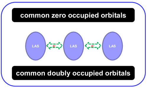
Figure 1: Illustration of local active spaces (LAS) in terms of LMOs.

Absolute overlaps between the six occupied pre-LMOs and all occupied molecular HF-LMOs for (C4SH3)-(CH2)10-(C4SH3) 1 2 3 4 5 6 $\cdots$^b 1 0.996 0.000 0.000 0.000 0.000 0.032 $\cdots$ 2 0.000 0.996 0.000 0.000 0.032 0.000 $\cdots$ 3 0.032 0.000 0.992 0.032 0.032 0.000 $\cdots$ 4 0.000 0.000 0.000 0.992 0.000 0.032 $\cdots$ 5 0.000 0.000 0.000 0.000 0.986 0.000 $\cdots$ 6 0.000 0.032 0.032 0.000 0.000 0.986 $\cdots$ 0.992^c 0.992^c 0.985^c 0.985^c 0.974^c 0.974^c $\cdots$

• Five $n\textrm{p}_{z}$ (n = 2 for C and 3 for S) orbitals from each of the terminal 5-membered rings C4S.

• Columns (core orbitals) with values smaller than 0.009.

• Occupation number.

Absolute overlaps between the four unoccupied pre-LMOs and all unoccupied molecular HF-LMOs for (C4SH3)-(CH2)10-(C4SH3)              1       2       3       4       $\cdots$^b       1       0.894       0.000       0.032       0.000       $\cdots$       2       0.000       0.894       0.000       0.032       $\cdots$       3       0.032       0.000       0.864       0.000       $\cdots$       4       0.000       0.032       0.000       0.864       $\cdots$       0.801^c       0.801^c       0.748^c       0.748^c       $\cdots$

• Five $n\textrm{p}_{z}$ (n = 2 for C and 3 for S) orbitals from each of the terminal 5-membered rings C4S.

• Columns (virtual orbitals) with values smaller than 0.060.

• Occupation number.

Absolute overlaps between the six occupied pre-CMOs and all occupied molecular HF-CMOs for (C4SH3)-(CH2)10-(C4SH3) 1 2 3 4 5 6 7 8 9 10 $\cdots$^b 1 0.032 0.000 0.055 0.000 0.543 0.506 0.404 0.305 0.279 0.205 $\cdots$ 2 0.000 0.032 0.000 0.055 0.539 0.510 0.407 0.302 0.277 0.205 $\cdots$ 3 0.809 0.581 0.032 0.000 0.000 0.000 0.000 0.000 0.000 0.000 $\cdots$ 4 0.581 0.809 0.000 0.032 0.000 0.000 0.000 0.000 0.000 0.000 $\cdots$ 5 0.032 0.000 0.931 0.173 0.063 0.134 0.045 0.134 0.100 0.118 $\cdots$ 6 0.000 0.032 0.173 0.931 0.063 0.134 0.045 0.134 0.100 0.118 $\cdots$ 0.993^c 0.993^c 0.900^c 0.900^c 0.593^c 0.552^c 0.333^c 0.220^c 0.175^c 0.112^c $\cdots$

• Five $n\textrm{p}_{z}$ (n = 2 for C and 3 for S) orbitals from each of the terminal 5-membered rings C4S.

• Columns (core orbitals) with values smaller than 0.025.

• Occupation number.

Absolute overlaps between the four unoccupied pre-CMOs and all unoccupied molecular HF-CMOs for (C4SH3)-(CH2)10-(C4SH3) 1 2 3 4 5 6 7 8 9 $\cdots$^b 1 0.709 0.608 0.032 0.105 0.045 0.126 0.000 0.032 0.055 $\cdots$ 2 0.608 0.709 0.032 0.105 0.045 0.126 0.000 0.032 0.055 $\cdots$ 3 0.089 0.077 0.586 0.559 0.344 0.261 0.161 0.158 0.145 $\cdots$ 4 0.077 0.089 0.586 0.560 0.344 0.261 0.161 0.158 0.145 $\cdots$ 0.886^c 0.886^c 0.688^c 0.649^c 0.240^c 0.168^c 0.052^c 0.052^c 0.048^c $\cdots$

• Five $n\textrm{p}_{z}$ (n = 2 for C and 3 for S) orbitals from each of the terminal 5-membered rings C4S.

• Columns (virtual orbitals) with values smaller than 0.011.

• Occupation number.

2.2 Subspace Matching

Given the guess orbitals $\{\psi_{p}^{\mathrm{Y}(0)}\}_{p=1}^{N_{\mathrm{orb}}}$ ($\mathrm{Y}=\mathrm{LMO},\mathrm{CMO}$), we are ready to perform the CASSCF calculation. Noticing that each iteration $k$ will generate delocalized CMOs $\{\psi_{i}^{\mathrm{CMO}(k)}\}_{i=1}^{N_{\mathrm{orb}}}$ and a proper reassignment of the core, active and virtual spaces has to be performed, we first calculate the occupation numbers of all $\{\psi_{i}^{\mathrm{CMO}(k)}\}_{i=1}^{N_{\mathrm{orb}}}$ in the core space $\{\psi_{p}^{\mathrm{Y}(k-1)}\}_{i=1}^{N_{\mathrm{c}}}$ of the previous iteration (cf. Eq. (12)), so as to identify the core orbitals $\{\psi_{i}^{\mathrm{CMO}(k)}\}_{p=1}^{N_{\mathrm{c}}}$ of the present iteration with the largest $N_{\mathrm{c}}$ occupation numbers $\{n_{\mathrm{c},i}\}_{i=1}^{N_{\mathrm{c}}}$. Then, the occupation numbers of the remaining $\{\psi_{i}^{\mathrm{CMO}(k)}\}_{i=N_{\mathrm{c}}+1}^{N_{\mathrm{orb}}}$ in the active space $\{\psi_{p}^{\mathrm{Y}(k-1)}\}_{p=N_{\mathrm{c}}+1}^{N_{\mathrm{c}}+K}$ are calculated to identify the $K$ active orbitals, again with the largest occupation numbers $\{n_{\mathrm{a},i}\}_{i=1}^{K}$. The left are obviously virtual orbitals. In case that some $\{n_{\mathrm{a},j}\}$ are very close to the smallest of $\{n_{\mathrm{a},i}\}_{i=1}^{K}$, it would indicate the prechosen AOs/pFLMOs are not enough and should hence be expanded. As a matter of fact, even in this case, the calculation need not be terminated but can still proceed ahead by just putting such orbitals into the active space, which will be stabilized in subsequent iterations. This way, the orbitals of two adjacent iterations are best matched. To localize the CASSCF-CMOs, they are first expanded as

$$(\psi_{\mathrm{c}}^{\mathrm{CMO}(k)},\psi_{\mathrm{a}}^{\mathrm{CMO}(k)},\psi_{\mathrm{v}}^{\mathrm{CMO}(k)})=(\psi_{\mathrm{c}}^{\mathrm{Y}(k-1)},\psi_{\mathrm{a}}^{\mathrm{Y}(k-1)},\psi_{\mathrm{v}}^{\mathrm{Y}(k-1)})\begin{pmatrix}\mathbf{C}_{\mathrm{cc}}&\mathbf{C}_{\mathrm{ca}}&\mathbf{C}_{\mathrm{cv}}\\ \mathbf{C}_{\mathrm{ac}}&\mathbf{C}_{\mathrm{aa}}&\mathbf{C}_{\mathrm{av}}\\ \mathbf{C}_{\mathrm{vc}}&\mathbf{C}_{\mathrm{va}}&\mathbf{C}_{\mathrm{vv}}\end{pmatrix},$$ (16)

where $\mathbf{C}_{\mathrm{xy}}=\langle\psi_{\mathrm{x}}^{\mathrm{Y}(k-1)}|\psi_{\mathrm{y}}^{\mathrm{CMO}(k)}\rangle$ ($\mathrm{x},\mathrm{y}=\mathrm{c},\mathrm{a},\mathrm{v}$). The $\mathbf{T}$ matrix (4) can then be constructed so as to transform $\{\psi_{i}^{\mathrm{CMO}(k)}\}_{i=1}^{N_{\mathrm{orb}}}$ to $\{\psi_{i}^{\mathrm{LMO}(k)}\}_{i=1}^{N_{\mathrm{orb}}}$ in view of the relation (5). Since the couplings between LMOs are much weaker than those between CMOs, generating CASSCF-LMOs in each iteration can typically facilitate the convergence. As can be seen from Tables 3.2 and 2.2, the converged CASSCF(12,10)-LMOs/CMOs do match the guess LMOs/CMOs for the case of (C4SH3)-(CH2)10-(C4SH3).

Absolute overlaps between the initial and final CAS(12,10)-LMOs of (C4SH3)-(CH2)10-(C4SH3) 1 2 3 4 5 6 7 8 9 10 1 0.996 0.000 0.008 0.000 0.003 0.000 0.000 0.011 0.000 0.006 2 0.000 0.996 0.000 0.008 0.000 0.003 0.011 0.000 0.006 0.000 3 0.004 0.000 0.998 0.000 0.001 0.000 0.000 0.003 0.000 0.014 4 0.000 0.004 0.000 0.998 0.000 0.001 0.003 0.000 0.014 0.000 5 0.000 0.000 0.001 0.000 0.999 0.000 0.000 0.001 0.000 0.011 6 0.000 0.000 0.000 0.001 0.000 0.999 0.001 0.000 0.011 0.000 7 0.000 0.013 0.000 0.003 0.000 0.002 0.869 0.000 0.015 0.000 8 0.013 0.000 0.003 0.000 0.002 0.000 0.000 0.869 0.000 0.015 9 0.000 0.008 0.000 0.016 0.000 0.013 0.005 0.000 0.863 0.000 10 0.008 0.000 0.016 0.000 0.013 0.000 0.000 0.005 0.000 0.863

Absolute overlaps between the initial and final CAS(12,10)-CMOs of (C4SH3)-(CH2)10-(C4SH3) 1 2 3 4 5 6 7 8 9 10 1 0.997 0.000 0.001 0.000 0.001 0.000 0.000 0.000 0.000 0.000 2 0.000 0.997 0.001 0.002 0.000 0.000 0.000 0.000 0.000 0.000 3 0.011 0.001 0.987 0.001 0.001 0.000 0.000 0.000 0.000 0.000 4 0.002 0.010 0.001 0.987 0.000 0.001 0.000 0.000 0.000 0.000 5 0.003 0.000 0.005 0.001 0.999 0.000 0.000 0.000 0.000 0.000 6 0.000 0.003 0.000 0.005 0.000 0.999 0.000 0.000 0.000 0.000 7 0.000 0.000 0.000 0.000 0.000 0.000 0.995 0.000 0.000 0.000 8 0.000 0.000 0.000 0.000 0.000 0.000 0.000 0.995 0.000 0.000 9 0.000 0.000 0.000 0.000 0.000 0.000 0.005 0.000 0.991 0.000 10 0.000 0.000 0.000 0.000 0.000 0.000 0.000 0.004 0.000 0.991

3 Illustrative examples

Except for the multi-state CASPT2⁶² calculations performed with the Molcas program package⁶³, all calculations were carried out with the BDF program package^{64, 65, 66, 67, 68, 69}. In particular, the Xi’an-CI module⁶⁹ in BDF was used to do the multi-state NEVPT2⁷⁰ and SDSPT2^{71, 72} calculations. The valence AOs were generated by SCF calculations of spherical, unpolarized atomic configurations with the same basis functions as used for molecular calculations. Local orientations of the AOs are taken care of automatically.

3.1 C-H bond breaking of ethylene

As a first application of the proposed $\mathbbm{i}$CAS approach, we examine the breaking of one C-H bond of ethylene, with the lengths of the other three C-H bonds, that of the C-C bond and the $\angle$HCH angle set to 1.085 Å, 1.339 Å and 124.8^∘, respectively. The basis set is ANO-RCC-VDZP⁷³. Intuitively, the breaking of a single $\sigma$-bond requires only a minimal CAS, i.e., two electrons in $\sigma$ and $\sigma^{\ast}$. However, this picture holds only when $\sigma$ and $\sigma^{\ast}$ are the highest occupied (HOMO) and lowest unoccupied (LUMO) molecular orbitals, respectively, during the whole dissociation process. As can be seen from Fig. 2, the $\sigma$ orbital is actually the HOMO-1 (lower than $\pi$) for distances shorter than $2.0$ Å and becomes the HOMO only beyond this distance. That is, there exists a swap of $\sigma$ and $\pi$ orbitals in the CAS(2,2) across this point. Consequently, the CMO-CAS(2,2) potential energy curve (PEC) is discontinuous nearby $2.0$ Å, as can be seen from Fig. 3. A smooth PEC can of course be reproduced by taking all the four frontier orbitals ($\sigma$, $\pi$, $\sigma^{\ast}$ and $\pi^{\ast}$) as active orbitals, i.e., CAS(4,4). As pointed out by Malrieu long ago⁷⁴, the CAS(2,2) calculation can also produce a smooth PEC if localized $\sigma$ and $\sigma^{\ast}$ orbitals are used throughout. This is indeed confirmed here by the present LMO-$\mathbbm{i}$CAS(2,2). Interestingly, the present CMO-$\mathbbm{i}$CAS(2,2), imposed by two pre-CMOs formed by C$2\textrm{p}_{x}$ and H$1\textrm{s}$, can also pick up the two right active orbitals and hence produces the same PEC as LMO-$\mathbbm{i}$CAS(2,2). The same findings hold also for the simultaneous breaking of two and even four C-H bonds of ethylene, as can be seen from Figs. 4 to 7. Although this example is very simple, it does reflect an important merit of $\mathbbm{i}$CAS: the active space spanned by the prechosen AOs hold the same for all geometries.

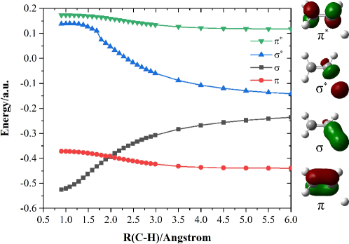
Figure 2: Energies of frontier HF orbitas for the C-H bond breaking of ethylene.

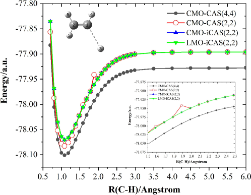
Figure 3: Potential energy curves for the breaking of single C-H bond of ethylene.

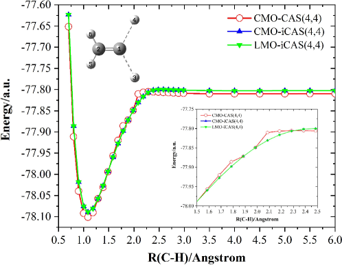
Figure 4: Potential energy curves for the simultaneous breaking of the two terminal C-H bonds of ethylene.

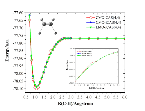
Figure 5: Potential energy curves for the simultaneous breaking of the two cis C-H bonds of ethylene.

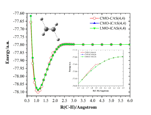
Figure 6: Potential energy curves for the simultaneous breaking of the two trans C-H bonds of ethylene.

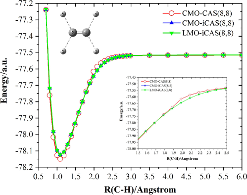
Figure 7: Potential energy curves for the simultaneous breaking of four C-H bonds of ethylene.

3.2 Electronic Structure of Co^III(diiminato)(NPh)

As a more stringent test of $\mathbbm{i}$CAS, we investigate the spin-state energetics of the low-coordinate imido complex Co^III(diiminato)(NPh), which is a simplified model of diamagnetic complex Co^III(nacnac)(NAd) [NB: nacnac=an anion of 2,4-bis(2,6-dimethylphenylimido) pentane; Ad=1-adamantyl]⁷⁵. The density functional theory study ⁷⁶ shows that there should be low-lying paramagnetic excited states besides the diamagnetic ground state, which has been calibrated by CAS(10,10)-based CASPT2⁷⁷. The major concern here is how to construct an appropriate CAS. On the practical side, the spin-free exact two-component (sf-X2C) Hamiltonian^{78, 79} in conjunction with the ANO-RCC-VDZP basis sets (Co/5s4p2d1f; N,C/3s2p1d; H/2s1p)⁷³ (as used in Ref. 77) is employed here. Twenty-nine core orbitals are frozen in the treatment of dynamic correlation, leaving in total 134 correlated electrons. In the CASPT2 calculations (with the spin-free Douglas-Kroll-Hess (DKH) Hamiltonian⁸⁰), an imaginary level shift of 0.1 is used to remove intruder states.

The singlet ground state geometry of Co^III(diiminato)(NPh) was optimized with sf-X2C-PBE0/def2-SVP^{81, 82}, without symmetry restrictions. As can be seen from Fig. 8, the Co atom is located almost at the center of the molecular skeleton, the imido nitrogen (N${}_{\textrm{imido}}$) is on the y axis, the 1,3-propanediiminato and phenylimido groups are in the xy plane, whereas the two terminal phenyl groups are perpendicular to the xy plane (see Supporting Information for the Cartesian coordinates). The crucial coordinate of Co^III(diiminato)(NPh) is the Co-N${}_{\textrm{imido}}$ bond, which was optimized to be 1.612 Å, very close to the CASPT2 value of 1.632 Å⁷⁷.

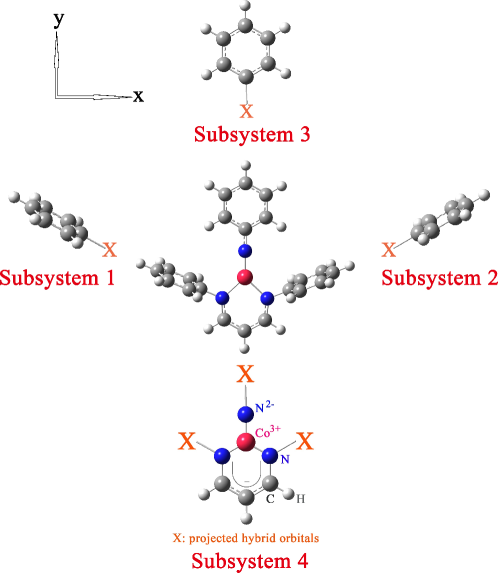
Figure 8: Fragmentation of Co^III(diiminato)(NPh).

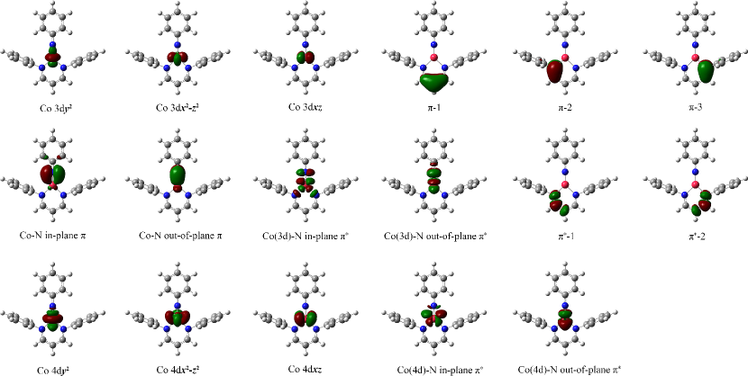
Figure 9: Automatically selected initial 17 active LMOs of singlet Co^III(diiminato)(NPh). Co-N is the shorthand notation of Co-N${}_{\textrm{imido}}$.

To initiate the “top-down, least-change” localization procedure (see Sec. 2.1), the molecule is partitioned into four fragments (see Fig. 8), with the dangling bonds saturated with the modified⁸³ PHO (projected hybrid orbital) boundary atoms⁸⁴. While subsystems 1-3 are obviously closed-shell systems, subsystem 4 can be in singlet, triplet or quintet. After the HF/ROHF calculations of these subsystems, the orthonormal pFLMOs are generated^{55, 56}, which are taken as the initial guess for the HF/ROHF calculations of the whole systems. The FLMOs are finally generated according to the “top-down, least-change” scheme. Since such FLMOs have one-to-one correspondence with the pFLMOs, the active orbitals can be chosen simply from the subsystem pFLMOs. However, to make the $\mathbbm{i}$CAS calculations “more difficult”, we still start with valence AOs. Looking at the chemical structure of the system, it should be easy to guess that, apart from the five 3d orbitals of Co, the five 2p_z orbitals of the C and N atoms of the 5-membered ring as well as the 2p_x and 2p_z of N${}_{\textrm{imido}}$ are most relevant for the chemical environment of Co, since the 2p_y orbital of N${}_{\textrm{imido}}$ participates in the bonding with the 6-membered ring. In addition to these valence AOs, the five 4d orbitals of Co can further be included to account for the so-called “double d-shell effect” resulting from physical intuitions⁸⁵. In essence, putting Co 4d into the active space amounts to shifting the inaccurate, perturbative treatment of their radial correlation effect to the exact, variational treatment. We then have in total 17 valence AOs (and hence 17 pre-LMOs/CMOs) along with 16 active electrons (6 for Co³⁺ (3d⁶), 6 for the anionic 5-membered ring, and 4 for $:$N${}_{\textrm{imido}}^{2-}$) according to minimal chemical and physical intuitions. Taking the 8 doubly occupied and 9 unoccupied pre-LMOs as probes, precisely 17 HF-LMOs (see Fig. 9) can be selected as initial guess for $\mathbbm{i}$CAS(16,17). As can be seen from Tables 3.2 and 3.2, the large absolute overlaps between the pre-LMOs and HF-LMOs do support the selection. The same findings also hold for the triplet and quintet states (see Supporting Information). Nevertheless, the CAS(16,17) calculations are too expensive (which, however, can readily be performed with the iCISCF algorithm⁴⁴ that employs the selected iterative configuration interaction (iCI)^{86, 87, 88} as the CAS solver). The first attempt to reduce CAS(16,17) is to exclude the five 2p_z orbitals of the 5-membered ring, thereby leading to CAS(10,12). As a matter of fact, this amounts just to deleting from Fig. 9 as well as Tables 3.2 and 3.2 the $\pi-1$, $\pi-2$, $\pi-2$, $\pi^{\ast}-1$, and $\pi^{\ast}-2$ orbitals that are localized on the 5-membered ring. It was also attempted⁷⁷ to further remove the 4d_xy and 4d_yz orbitals from CAS(10,12), for the 3d${}_{y^{2}}$, 3d${}_{x^{2}-z^{2}}$ and 3d_xz orbitals are doubly occupied in the singlet ground state, such that only 4d${}_{y^{2}}$, 4d${}_{x^{2}-z^{2}}$ and 4d_xz are relevant for the “double d-shell effect”. A more dramatic simplification is to exclude all the 4d orbitals from CAS(10,12), thereby leading to CAS(10,7). These two cases amount to deleting from Fig. 9 the last two and five orbitals involving Co 4d, respectively.

Having prepared the initial guess, two-state averaged $\mathbbm{i}$CAS (SA2-$\mathbbm{i}$CAS) calculations are performed for each spin state. As can be seen from Table 3.2, the converged $\mathbbm{i}$CAS(10,12) orbitals are indeed very close to the initial ones. Again, the same findings also hold for the triplet and quintet states (see Supporting Information). For completeness, the leading configurations of the CAS wave functions are given in Table 3.2. The vertical excitation energies calculated by $\mathbbm{i}$CAS, CASPT2, NEVPT2, and SDSPT2 are documented in Table 3.2. It can first be seen that, at the CASSCF level, CAS(10,7) is far from being sufficient: it even predicts that the two nearly degenerate ${}^{3}A$ states are lower than the lowest singlet state by 0.3 eV; CAS(10,10) is also imperfect: although it does predict correctly the ground state⁷⁵, the excitation energies of the remaining states are too high, by 0.3 to 0.6 eV. In contrast, CAS(10,12) is essentially saturated, with the predicted excitation energies differing from the CAS(16,17) ones by at most 0.15 eV. It can also be seen that the imperfections in CAS(10,10) and even CAS(10,7) are essentially removed by the subsequent CASPT2/NEVPT2/SDSPT2 treatment of dynamic correlation, indicating that the “double d-shell effect” plays a very minor role here. As a matter of fact, there exists very little dynamic correlation (ca. 0.1 eV) beyond CAS(10,12), as compared with CAS(10,12)-NEVPT2/SDSPT2. This can be explained by the fact that the spin states investigated here all arise from spin flips within the same Co 3d manifold (cf. Table 3.2), for which dynamic correlation effects are largely cancelled out for the relative energies. The situation may be different for states involving changes in the occupations of $n$d (and $n$f) orbitals, where substantial differential correlation effects may be experienced. Note also that there exist substantial differences (ca. 0.4 eV) between the present and the previous⁷⁷ CAS(10,10)-CASPT2 excitation energies for the two ${}^{5}A$ states. Although the same CASPT2 code⁶³ is used in both cases, the present calculation takes the SA2-iCAS(10,10) LMOs as input.

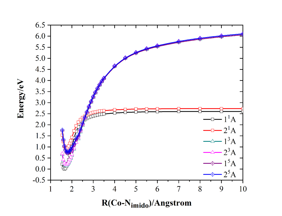
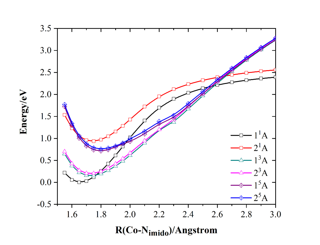
(a) full	(b) zoom-in

Figure 10: sf-X2C-SA2-$\mathbbm{i}$CAS(10,12)/ANO-RCC-VDZP potential energy curves for the rigid dissociation of Co-N${}_{\textrm{imido}}$ in Co^III(diiminato)(NPh).

To further examine the efficacy of $\mathbbm{i}$CAS in maintaining the same CAS for all geometries, the rigid stretching of the Co-N${}_{\textrm{imido}}$ bond (keeping the other atoms fixed) is considered. The SA2-$\mathbbm{i}$CAS(10,12) PECs for the six states are plotted in Fig. 10. The smoothness of the PECs is obvious. While the Co-N${}_{\textrm{imido}}$ bond in the $1^{1}A$ and $2^{1}A$ states starts to dissociate around 4.5 Å, that in the four triplet and quintet states does not even up to 10 Å. It is also of interest to see that the four triplet and quintet states become degenerate beyond 2.3 Å. Finally, the equilibrium Co-N${}_{\textrm{imido}}$ distances $R_{e}$ are given in Table 3.2. Again, there exist significant differences (ca. 0.04 Å) between the present and the previous⁷⁷ CASPT2 values for $R_{e}$, due to the use of different CAS(10,10) orbitals.

Absolute overlaps between the eight doubly occupied pre-LMOs and all doubly occupied molecular HF-LMOs for singlet Co^III(diiminato)(NPh) 1 2 3 4 5 6 7 8 9 $\cdots$^b $b_{\perp}$ 0.960 0.000 0.000 0.000 0.000 0.000 0.000 0.000 0.000 $\cdots$ $b_{\parallel}$ 0.000 0.954 0.000 0.000 0.000 0.000 0.000 0.000 0.000 $\cdots$ Co $\textrm{3d}_{xz}$ 0.000 0.000 0.999 0.000 0.000 0.000 0.000 0.000 0.000 $\cdots$ Co $\textrm{3d}_{x^{2}-z^{2}}$ 0.000 0.000 0.000 0.721 0.507 0.000 0.000 0.000 0.265 $\cdots$ Co $\textrm{3d}_{y^{2}}$ 0.000 0.000 0.000 0.550 0.700 0.000 0.000 0.000 0.389 $\cdots$ $\pi$-1 0.032 0.000 0.000 0.000 0.000 0.990 0.000 0.000 0.000 $\cdots$ $\pi$-2 0.000 0.000 0.000 0.000 0.000 0.000 0.968 0.000 0.000 $\cdots$ $\pi$-3 0.000 0.000 0.000 0.000 0.000 0.000 0.000 0.968 0.000 $\cdots$ 0.923^c 0.910^c 0.999^c 0.822^c 0.747^c 0.980^c 0.937^c 0.937^c 0.221^c $\cdots$

• $b_{\parallel}$ and $b_{\perp}$ denote Co(3d)-N${}_{\textrm{imido}}$ in plane $\pi$ and out-of-plane $\pi$; $\pi$-1, $\pi$-2 and $\pi$-3 correspond to localized $\pi$ of 1,3-propanediiminato.

• Columns (core orbitals) with values smaller than 0.059.

• Occupation number.

Absolute overlaps between the nine unoccupied pre-LMOs and all unoccupied molecular HF-LMOs for singlet Co^III(diiminato)(NPh) 1 2 3 4 5 6 7 8 9 10 $\cdots$^b $b_{\perp}^{\ast}$ 0.861 0.000 0.000 0.000 0.000 0.158 0.000 0.000 0.000 0.224 $\cdots$ $b_{\parallel}^{\ast}$ 0.000 0.742 0.000 0.000 0.000 0.000 0.161 0.000 0.000 0.000 $\cdots$ Co $\textrm{4d}_{y^{2}}$ 0.000 0.000 0.599 0.395 0.000 0.000 0.000 0.000 0.000 0.000 $\cdots$ Co $\textrm{4d}_{x^{2}-z^{2}}$ 0.000 0.000 0.452 0.724 0.000 0.032 0.000 0.000 0.000 0.187 $\cdots$ Co $\textrm{4d}_{xz}$ 0.000 0.000 0.000 0.000 0.913 0.000 0.000 0.000 0.000 0.179 $\cdots$ $\tilde{b}_{\perp}^{\ast}$ 0.130 0.000 0.000 0.084 0.000 0.901 0.000 0.000 0.000 0.105 $\cdots$ $\tilde{b}_{\parallel}^{\ast}$ 0.000 0.392 0.000 0.000 0.000 0.000 0.778 0.000 0.000 0.000 $\cdots$ $\pi^{\ast}$-1 0.000 0.000 0.000 0.000 0.000 0.000 0.000 0.866 0.032 0.032 $\cdots$ $\pi^{\ast}$-2 0.000 0.000 0.000 0.045 0.000 0.000 0.000 0.032 0.866 0.032 $\cdots$ 0.758^c 0.705^c 0.563^c 0.689^c 0.833^c 0.838^c 0.632^c 0.751^c 0.751^c 0.130^c $\cdots$

• $b_{\parallel}^{\ast}$ and $b_{\perp}^{\ast}$ denote Co(3d)-N${}_{\textrm{imido}}$ in plane and out-of-plane $\pi^{\ast}$; $\tilde{b}_{\parallel}^{\ast}$ and $\tilde{b}_{\perp}^{\ast}$ denote Co(4d)-N${}_{\textrm{imido}}$ in plane and out-of-plane $\pi^{\ast}$; $\pi^{\ast}$-1 and $\pi^{\ast}$-2 correspond to localized $\pi^{\ast}$ of 1,3-propanediiminato.

• Columns (virtual orbitals) with values smaller than 0.073.

• Occupation number.

Absolute overlaps between the initial and final SA2-$\mathbbm{i}$CAS(10,12) LMOs for singlet Co^III(diiminato)(NPh) 1 2 3 4 5 6 7 8 9 10 11 12 Co $\textrm{3d}_{y^{2}}$ 0.874 0.000 0.001 0.000 0.000 0.000 0.000 0.000 0.014 0.000 0.000 0.000 Co $\textrm{3d}_{x^{2}-z^{2}}$ 0.001 0.911 0.000 0.000 0.000 0.000 0.000 0.000 0.002 0.000 0.000 0.003 Co $\textrm{3d}_{xz}$ 0.001 0.000 0.998 0.000 0.001 0.000 0.000 0.000 0.000 0.005 0.000 0.000 $b_{\parallel}$ 0.000 0.000 0.000 0.978 0.000 0.000 0.002 0.000 0.000 0.000 0.008 0.000 $b_{\perp}$ 0.000 0.000 0.000 0.000 0.989 0.008 0.000 0.012 0.000 0.000 0.000 0.005 $b_{\perp}^{\ast}$ 0.000 0.000 0.000 0.008 0.000 0.886 0.000 0.014 0.000 0.000 0.000 0.021 $b_{\parallel}^{\ast}$ 0.000 0.002 0.000 0.000 0.000 0.000 0.894 0.001 0.000 0.000 0.121 0.001 Co $\textrm{4d}_{y^{2}}$ 0.000 0.000 0.014 0.000 0.002 0.000 0.000 0.715 0.003 0.001 0.000 0.017 Co $\textrm{4d}_{x^{2}-z^{2}}$ 0.000 0.000 0.000 0.005 0.003 0.021 0.001 0.040 0.863 0.001 0.000 0.017 Co $\textrm{4d}_{xz}$ 0.005 0.000 0.000 0.000 0.000 0.000 0.000 0.000 0.001 0.892 0.000 0.001 $\tilde{b}_{\perp}^{\ast}$ 0.000 0.000 0.000 0.012 0.000 0.014 0.001 0.003 0.003 0.000 0.876 0.040 $\tilde{b}_{\parallel}^{\ast}$ 0.000 0.008 0.000 0.000 0.000 0.000 0.121 0.003 0.000 0.000 0.000 0.753

Leading configurations of HF/ROHF and $\mathbbm{i}$CAS calculations of Co^III(diiminato)(NPh) state main configuration^a energy (eV)/weight^b HF/ROHF 1¹A $(\textrm{3d}_{y^{2}})^{2}(\textrm{3d}_{x^{2}-z^{2}})^{2}(\textrm{3d}_{xz})^{2}(b_{\parallel})^{2}(b_{\perp})^{2}$ 0.00 1³A $(\textrm{3d}_{y^{2}})^{2}(\textrm{3d}_{x^{2}-z^{2}})^{2}(\textrm{3d}_{xz})^{2}(b_{\parallel})^{2}(b_{\perp})^{1}(b_{\perp}^{\ast})^{1}$ -1.40 1⁵A $(\textrm{3d}_{y^{2}})^{1}(\textrm{3d}_{x^{2}-z^{2}})^{2}(\textrm{3d}_{xz})^{1}(b_{\parallel})^{2}(b_{\perp})^{2}(b_{\perp}^{\ast})^{1}(b_{\parallel}^{\ast})^{1}$ -3.34 $\mathbbm{i}$CAS(10,7) 1¹A $(\textrm{3d}_{y^{2}})^{2}(\textrm{3d}_{x^{2}-z^{2}})^{2}(\textrm{3d}_{xz})^{2}(b_{\parallel})^{2}(b_{\perp})^{2}(b_{\perp}^{\ast})^{0}(b_{\parallel}^{\ast})^{0}$ 0.761 2¹A $(\textrm{3d}_{y^{2}})^{2}(\textrm{3d}_{x^{2}-z^{2}})^{2}(\textrm{3d}_{xz})^{2}(b_{\parallel})^{2}(b_{\perp})^{1}(b_{\perp}^{\ast})^{1}(b_{\parallel}^{\ast})^{0}$ 0.804 1³A $(\textrm{3d}_{y^{2}})^{2}(\textrm{3d}_{x^{2}-z^{2}})^{1}(\textrm{3d}_{xz})^{2}(b_{\parallel})^{2}(b_{\perp})^{2}(b_{\perp}^{\ast})^{1}(b_{\parallel}^{\ast})^{0}$ 0.738 2³A $(\textrm{3d}_{y^{2}})^{2}(\textrm{3d}_{x^{2}-z^{2}})^{2}(\textrm{3d}_{xz})^{1}(b_{\parallel})^{2}(b_{\perp})^{2}(b_{\perp}^{\ast})^{1}(b_{\parallel}^{\ast})^{0}$ 0.740 1⁵A $(\textrm{3d}_{y^{2}})^{1}(\textrm{3d}_{x^{2}-z^{2}})^{1}(\textrm{3d}_{xz})^{2}(b_{\parallel})^{2}(b_{\perp})^{2}(b_{\perp}^{\ast})^{1}(b_{\parallel}^{\ast})^{1}$ 0.820 2⁵A $(\textrm{3d}_{y^{2}})^{1}(\textrm{3d}_{x^{2}-z^{2}})^{2}(\textrm{3d}_{xz})^{1}(b_{\parallel})^{2}(b_{\perp})^{2}(b_{\perp}^{\ast})^{1}(b_{\parallel}^{\ast})^{1}$ 0.822 $\mathbbm{i}$CAS(10,10) 1¹A $(\textrm{3d}_{y^{2}})^{2}(\textrm{3d}_{x^{2}-z^{2}})^{2}(\textrm{3d}_{xz})^{2}(b_{\parallel})^{2}(b_{\perp})^{2}(b_{\perp}^{\ast})^{0}(b_{\parallel}^{\ast})^{0}(\textrm{4d}_{y^{2}})^{0}(\textrm{4d}_{x^{2}-z^{2}})^{0}(\textrm{4d}_{xz})^{0}$ 0.771 2¹A $(\textrm{3d}_{y^{2}})^{2}(\textrm{3d}_{x^{2}-z^{2}})^{2}(\textrm{3d}_{xz})^{2}(b_{\parallel})^{2}(b_{\perp})^{1}(b_{\perp}^{\ast})^{1}(b_{\parallel}^{\ast})^{0}(\textrm{4d}_{y^{2}})^{0}(\textrm{4d}_{x^{2}-z^{2}})^{0}(\textrm{4d}_{xz})^{0}$ 0.812 1³A $(\textrm{3d}_{y^{2}})^{2}(\textrm{3d}_{x^{2}-z^{2}})^{1}(\textrm{3d}_{xz})^{2}(b_{\parallel})^{2}(b_{\perp})^{2}(b_{\perp}^{\ast})^{1}(b_{\parallel}^{\ast})^{0}(\textrm{4d}_{y^{2}})^{0}(\textrm{4d}_{x^{2}-z^{2}})^{0}(\textrm{4d}_{xz})^{0}$ 0.768 2³A $(\textrm{3d}_{y^{2}})^{2}(\textrm{3d}_{x^{2}-z^{2}})^{2}(\textrm{3d}_{xz})^{1}(b_{\parallel})^{2}(b_{\perp})^{2}(b_{\perp}^{\ast})^{1}(b_{\parallel}^{\ast})^{0}(\textrm{4d}_{y^{2}})^{0}(\textrm{4d}_{x^{2}-z^{2}})^{0}(\textrm{4d}_{xz})^{0}$ 0.769 1⁵A $(\textrm{3d}_{y^{2}})^{1}(\textrm{3d}_{x^{2}-z^{2}})^{1}(\textrm{3d}_{xz})^{2}(b_{\parallel})^{2}(b_{\perp})^{2}(b_{\perp}^{\ast})^{1}(b_{\parallel}^{\ast})^{1}(\tilde{b}_{\perp}^{\ast})^{0}(\textrm{4d}_{x^{2}-z^{2}})^{0}(\textrm{4d}_{xz})^{0}$ 0.909 2⁵A $(\textrm{3d}_{y^{2}})^{1}(\textrm{3d}_{x^{2}-z^{2}})^{2}(\textrm{3d}_{xz})^{1}(b_{\parallel})^{2}(b_{\perp})^{2}(b_{\perp}^{\ast})^{1}(b_{\parallel}^{\ast})^{1}(\tilde{b}_{\perp}^{\ast})^{0}(\textrm{4d}_{x^{2}-z^{2}})^{0}(\textrm{4d}_{xz})^{0}$ 0.904 $\mathbbm{i}$CAS(10,12) 1¹A $(\textrm{3d}_{y^{2}})^{2}(\textrm{3d}_{x^{2}-z^{2}})^{2}(\textrm{3d}_{xz})^{2}(b_{\parallel})^{2}(b_{\perp})^{2}(b_{\perp}^{\ast})^{0}(b_{\parallel}^{\ast})^{0}(\textrm{4d}_{y^{2}})^{0}(\textrm{4d}_{x^{2}-z^{2}})^{0}(\textrm{4d}_{xz})^{0}(\tilde{b}_{\perp}^{\ast})^{0}(\tilde{b}_{\parallel}^{\ast})^{0}$ 0.742 2¹A $(\textrm{3d}_{y^{2}})^{2}(\textrm{3d}_{x^{2}-z^{2}})^{2}(\textrm{3d}_{xz})^{2}(b_{\parallel})^{2}(b_{\perp})^{1}(b_{\perp}^{\ast})^{1}(b_{\parallel}^{\ast})^{0}(\textrm{4d}_{y^{2}})^{0}(\textrm{4d}_{x^{2}-z^{2}})^{0}(\textrm{4d}_{xz})^{0}(\tilde{b}_{\perp}^{\ast})^{0}(\tilde{b}_{\parallel}^{\ast})^{0}$ 0.778 1³A $(\textrm{3d}_{y^{2}})^{2}(\textrm{3d}_{x^{2}-z^{2}})^{1}(\textrm{3d}_{xz})^{2}(b_{\parallel})^{2}(b_{\perp})^{2}(b_{\perp}^{\ast})^{1}(b_{\parallel}^{\ast})^{0}(\textrm{4d}_{y^{2}})^{0}(\textrm{4d}_{x^{2}-z^{2}})^{0}(\textrm{4d}_{xz})^{0}(\tilde{b}_{\perp}^{\ast})^{0}(\tilde{b}_{\parallel}^{\ast})^{0}$ 0.771 2³A $(\textrm{3d}_{y^{2}})^{2}(\textrm{3d}_{x^{2}-z^{2}})^{2}(\textrm{3d}_{xz})^{1}(b_{\parallel})^{2}(b_{\perp})^{2}(b_{\perp}^{\ast})^{1}(b_{\parallel}^{\ast})^{0}(\textrm{4d}_{y^{2}})^{0}(\textrm{4d}_{x^{2}-z^{2}})^{0}(\textrm{4d}_{xz})^{0}(\tilde{b}_{\perp}^{\ast})^{0}(\tilde{b}_{\parallel}^{\ast})^{0}$ 0.760 1⁵A $(\textrm{3d}_{y^{2}})^{1}(\textrm{3d}_{x^{2}-z^{2}})^{1}(\textrm{3d}_{xz})^{2}(b_{\parallel})^{2}(b_{\perp})^{2}(b_{\perp}^{\ast})^{1}(b_{\parallel}^{\ast})^{1}(\textrm{4d}_{y^{2}})^{0}(\textrm{4d}_{x^{2}-z^{2}})^{0}(\textrm{4d}_{xz})^{0}(\tilde{b}_{\perp}^{\ast})^{0}(\tilde{b}_{\parallel}^{\ast})^{0}$ 0.834 2⁵A $(\textrm{3d}_{y^{2}})^{1}(\textrm{3d}_{x^{2}-z^{2}})^{2}(\textrm{3d}_{xz})^{1}(b_{\parallel})^{2}(b_{\perp})^{2}(b_{\perp}^{\ast})^{1}(b_{\parallel}^{\ast})^{1}(\textrm{4d}_{y^{2}})^{0}(\textrm{4d}_{x^{2}-z^{2}})^{0}(\textrm{4d}_{xz})^{0}(\tilde{b}_{\perp}^{\ast})^{0}(\tilde{b}_{\parallel}^{\ast})^{0}$ 0.832

• $b_{\parallel}$ ($b_{\parallel}^{\ast}$) and $b_{\perp}$ ($b_{\perp}^{\ast}$) denote Co(4d)-N${}_{\textrm{imido}}$ in plane and out-of-plane $\pi$ ($\pi^{\ast}$), respectively; $\tilde{b}_{\perp}^{\ast}$ denotes Co(4d)-N${}_{\textrm{imido}}$ out-of-plane $\pi^{\ast}$ with $\textrm{4d}_{yz}$ as the major.

• HF/ROHF total energies relative to the singlet (-2361.437053 a.u.); weights of leading configurations for CASSCF.

Vertical excitation energies (in eV) of Co^III(diiminato)(NPh) calculated at the singlet ground state geometry (see Supporting Information) $\mathbbm{i}$CAS^a CASPT2 NEVPT2 SDSPT2 state CAS1 CAS2 CAS3 CAS4^b CAS1 CAS2^c CAS3 CAS1 CAS2 CAS3 CAS1 CAS2 CAS3 1¹A 0.00 0.00 0.00 0.00 0.00 0.00(0.00) 0.00 0.00 0.00 0.00 0.00 0.00 0.00 2¹A 0.93 1.77 1.15 1.19 1.01 0.88(0.83) 1.01 1.14 0.86 1.03 1.14 0.89 1.04 1³A -0.37 0.57 0.30 0.43 0.34 0.24(0.11) 0.27 0.55 0.33 0.33 0.52 0.34 0.34 2³A -0.31 0.63 0.35 0.50 0.38 0.29(0.15) 0.32 0.60 0.37 0.38 0.57 0.37 0.38 1⁵A 0.26 1.65 1.19 1.35 1.01 0.91(0.59) 1.03 1.31 1.13 1.31 1.28 1.15 1.31 2⁵A 0.32 1.72 1.24 l.36 0.95 0.95(0.59) 1.08 1.37 1.14 1.35 1.34 1.16 1.35

• CAS1, CAS2, CAS3 and CAS4 denote CAS(10,7), CAS(10,10), CAS(10,12) and CAS(16,17), respectively.

• Calculated with the iCISCF approach⁴⁴.

• Values in parentheses are results from Ref. 77.

Equilibrium distances (in Å) for the rigid dissociation of Co-N${}_{\textrm{imido}}$ in Co^III(diiminato)(NPh)          state          $\mathbbm{i}$CAS(10,12)          CASPT2          NEVPT2          SDSPT2          1¹A          1.660          1.605          1.602          1.602          2¹A          1.752          1.697          1.697          1.697          1³A          1.743          1.651          1.649          1.651          2³A          1.743          1.651          1.649          1.651          1⁵A          1.798          1.706          1.743          1.743          2⁵A          1.798          1.706          1.743          1.743

4 Conclusions and outlook

An $\mathbbm{i}$CAS method has been proposed to serve as an initial step for describing strongly correlated systems of electrons. It has several features: (1) the active orbitals can be selected automatically by starting with prechosen valence/core atomic/fragmental orbitals. The only requirement lies in that such atomic/fragmental orbitals span a space that is sufficient for the target many-electron states, which hold for most organic molecules or transition metal complexes. (2) The CASSCF orbitals can readily be localized in each iteration so as to facilitate the matching of core, active and virtual subspaces. (3) The CAS can be maintained the same for all geometries, which is of vital importance for the scanning of potential energy surfaces. (4) Further combined with the iterative vector interaction (iVI) approach^{89, 90} for directly accessing interior roots of the CI eigenvalue problem, the CASSCF calculation can be dictated to converge to a predesignated chare/spin configuration composed of some special motifs (e.g., metal valence d/f orbitals, atomic core orbitals or aromatic rings), a point that is to be investigated in future though.

Data Availability Statement

The Cartesian coordinates of the Co^III(diiminato)(NPh) as well as various plots of the CASSCF orbitals are documented in the Supporting Information.

References

- Pulay and Hamilton 1988 Pulay, P.; Hamilton, T. P. UHF natural orbitals for defining and starting MC-SCF calculations. J. Chem. Phys. 1988, 88, 4926–4933
- Bofill and Pulay 1989 Bofill, J. M.; Pulay, P. The unrestricted natural orbital–complete active space (UNO–CAS) method: An inexpensive alternative to the complete active space–self-consistent-field (CAS–SCF) method. J. Chem. Phys. 1989, 90, 3637–3646
- Keller et al. 2015 Keller, S.; Boguslawski, K.; Janowski, T.; Reiher, M.; Pulay, P. Selection of active spaces for multiconfigurational wavefunctions. J. Chem. Phys. 2015, 142, 244104
- Abrams and Sherrill 2004 Abrams, M. L.; Sherrill, C. D. Natural orbitals as substitutes for optimized orbitals in complete active space wavefunctions. Chem. Phys. Lett. 2004, 395, 227–232
- Cheung et al. 1978 Cheung, L.; Sundberg, K.; Ruedenberg, K. Dimerization of carbene to ethylene. J. Am. Chem. Soc. 1978, 100, 8024–8025
- Roos et al. 1980 Roos, B. O.; Taylor, P. R.; Sigbahn, P. E. A complete active space SCF method (CASSCF) using a density matrix formulated super-CI approach. Chem. Phys. 1980, 48, 157–173
- Werner 1987 Werner, H.-J. Matrix-formulated direct multiconfiguration self-consistent field and multiconfiguration reference configuration-interaction methods. Adv. Chem. Phys. 1987, 69, 1–62
- Roos 1987 Roos, B. O. The complete active space self-consistent field method and its applications in electronic structure calculations. Adv. Chem. Phys. 1987, 69, 399–445
- Shepard 1987 Shepard, R. The multiconfiguration self-consistent field method. Adv. Chem. Phys 1987, 69, 63–200
- Schmidt and Gordon 1998 Schmidt, M. W.; Gordon, M. S. The construction and interpretation of MCSCF wavefunctions. Annu. Rev. Phys. Chem. 1998, 49, 233–266
- Szalay et al. 2012 Szalay, P. G.; Muller, T.; Gidofalvi, G.; Lischka, H.; Shepard, R. Multiconfiguration self-consistent field and multireference configuration interaction methods and applications. Chem. Rev. 2012, 112, 108–181
- Sun 2016 Sun, Q. Co-iterative augmented Hessian method for orbital optimization. arXiv preprint arXiv:1610.08423 2016,
- Kreplin et al. 2019 Kreplin, D. A.; Knowles, P. J.; Werner, H.-J. Second-order MCSCF optimization revisited. I. Improved algorithms for fast and robust second-order CASSCF convergence. J. Chem. Phys. 2019, 150, 194106
- Kreplin et al. 2020 Kreplin, D. A.; Knowles, P. J.; Werner, H.-J. MCSCF optimization revisited. II. Combined first- and second-order orbital optimization for large molecules. J. Chem. Phys. 2020, 152, 074102
- Yaffe and Goddard III 1976 Yaffe, L. G.; Goddard III, W. A. Orbital optimization in electronic wave functions; equations for quadratic and cubic convergence of general multiconfiguration wave functions. Phys. Rev. A 1976, 13, 1682
- Walch et al. 1983 Walch, S. P.; Bauschlicher Jr, C. W.; Roos, B. O.; Nelin, C. J. Theoretical evidence for multiple 3d bondig in the V2 and Cr2 molecules. Chem. Phys. Lett. 1983, 103, 175–179
- Clifford et al. 1996 Clifford, S.; Bearpark, M. J.; Robb, M. A. A hybrid MC-SCF method: generalised valence bond (GVB) with complete active space SCF (CASSCF). Chem. Phys. Lett. 1996, 255, 320–326
- Nakano and Hirao 2000 Nakano, H.; Hirao, K. A quasi-complete active space self-consistent field method. Chem. Phys. Lett. 2000, 317, 90–96
- Panin and Sizova 1996 Panin, A.; Sizova, O. Direct CI method in restricted configuration spaces. J. Comput. Chem. 1996, 17, 178–184
- Panin and Simon 1996 Panin, A.; Simon, K. Configuration interaction spaces with arbitrary restrictions on orbital occupancies. Int. J. Quantum Chem. 1996, 59, 471–475
- Ivanic 2003 Ivanic, J. Direct configuration interaction and multiconfigurational self-consistent-field method for multiple active spaces with variable occupations. I. Method. J. Chem. Phys. 2003, 119, 9364–9376
- Olsen et al. 1988 Olsen, J.; Roos, B. O.; Jørgensen, P.; Jensen, H. J. A. Determinant based configuration interaction algorithms for complete and restricted configuration interaction spaces. J. Chem. Phys. 1988, 89, 2185–2192
- Malmqvist et al. 1990 Malmqvist, P.-Å.; Rendell, A.; Roos, B. O. The restricted active space self-consistent-field method, implemented with a split graph unitary group approach. J. Phys. Chem. 1990, 94, 5477–5482
- Ma et al. 2011 Ma, D.; Li Manni, G.; Gagliardi, L. The generalized active space concept in multiconfigurational self-consistent field methods. J. Chem. Phys. 2011, 135, 044128
- Li Manni et al. 2013 Li Manni, G.; Ma, D.; Aquilante, F.; Olsen, J.; Gagliardi, L. SplitGAS method for strong correlation and the challenging case of Cr2. J. Chem. Theory Comput. 2013, 9, 3375–3384
- Vogiatzis et al. 2015 Vogiatzis, K. D.; Li Manni, G.; Stoneburner, S. J.; Ma, D.; Gagliardi, L. Systematic expansion of active spaces beyond the CASSCF limit: A GASSCF/SplitGAS benchmark study. J. Chem. Theory Comput. 2015, 11, 3010–3021
- Kim et al. 2015 Kim, I.; Parker, S. M.; Shiozaki, T. Orbital optimization in the active space decomposition model. J. Chem. Theory Comput. 2015, 11, 3636–3642
- Gidofalvi and Mazziotti 2008 Gidofalvi, G.; Mazziotti, D. A. Active-space two-electron reduced-density-matrix method: Complete active-space calculations without diagonalization of the N-electron Hamiltonian. J. Chem. Phys. 2008, 129, 134108
- Fosso-Tande et al. 2016 Fosso-Tande, J.; Nguyen, T.-S.; Gidofalvi, G.; DePrince, A. E. Large-Scale Variational Two-Electron Reduced-Density-Matrix-Driven Complete Active Space Self-Consistent Field Methods. J. Chem. Theory Comput. 2016, 12, 2260–2271
- Zgid and Nooijen 2008 Zgid, D.; Nooijen, M. The density matrix renormalization group self-consistent field method: Orbital optimization with the density matrix renormalization group method in the active space. J. Chem. Phys. 2008, 128, 144116
- Ghosh et al. 2008 Ghosh, D.; Hachmann, J.; Yanai, T.; Chan, G. K.-L. Orbital optimization in the density matrix renormalization group, with applications to polyenes and -carotene. J. Chem. Phys. 2008, 128, 144117
- Yanai et al. 2009 Yanai, T.; Kurashige, Y.; Ghosh, D.; Chan, G. K.-L. Accelerating convergence in iterative solution for large-scale complete active space self-consistent-field calculations. Int. J. Quantum Chem. 2009, 109, 2178–2190
- Ma and Ma 2013 Ma, Y.; Ma, H. Assessment of various natural orbitals as the basis of large active space density-matrix renormalization group calculations. J. Chem. Phys. 2013, 138, 224105
- Wouters et al. 2014 Wouters, S.; Bogaerts, T.; Van Der Voort, P.; Van Speybroeck, V.; Van Neck, D. Communication: DMRG-SCF study of the singlet, triplet, and quintet states of oxo-Mn (Salen). J. Chem. Phys. 2014, 140, 241103
- Ma et al. 2017 Ma, Y.; Knecht, S.; Keller, S.; Reiher, M. Second-order self-consistent-field density-matrix renormalization group. J. Chem. Theory Comput. 2017, 13, 2533–2549
- Sun et al. 2017 Sun, Q.; Yang, J.; Chan, G. K.-L. A general second order complete active space self-consistent-field solver for large-scale systems. Chem. Phys. Lett. 2017, 683, 291–299
- Thomas et al. 2015 Thomas, R. E.; Sun, Q.; Alavi, A.; Booth, G. H. Stochastic multiconfigurational self-consistent field theory. J. Chem. Theory Comput. 2015, 11, 5316–5325
- Li Manni et al. 2016 Li Manni, G.; Smart, S. D.; Alavi, A. Combining the complete active space self-consistent field method and the full configuration interaction quantum Monte Carlo within a super-CI framework, with application to challenging metal-porphyrins. J. Chem. Theory Comput. 2016, 12, 1245–1258
- Smith et al. 2017 Smith, J. E. T.; Mussard, B.; Holmes, A. A.; Sharma, S. Cheap and near exact CASSCF with large active spaces. J. Chem. Theory Comput. 2017, 13, 5468–5478
- Yao and Umrigar 2021 Yao, Y.; Umrigar, C. Orbital Optimization in Selected Configuration Interaction Methods. arXiv preprint arXiv:2104.02587 2021,
- Zimmerman and Rask 2019 Zimmerman, P. M.; Rask, A. E. Evaluation of full valence correlation energies and gradients. J. Chem. Phys. 2019, 150, 244117
- Levine et al. 2020 Levine, D. S.; Hait, D.; Tubman, N. M.; Lehtola, S.; Whaley, K. B.; Head-Gordon, M. CASSCF with Extremely Large Active Spaces Using the Adaptive Sampling Configuration Interaction Method. J. Chem. Theory Comput. 2020, 16, 2340–2354
- Park 2021 Park, J. W. Second-Order Orbital Optimization with Large Active Spaces Using Adaptive Sampling Configuration Interaction (ASCI) and Its Application to Molecular Geometry Optimization. J. Chem. Theory Comput. 2021,
- 44 Guo, Y.; Zhang, N.; Lei, Y.; Liu, W. iCISCF: Multiconfigurational self-consistent field theory based on iterative configuration interaction with selection. (unpublished)
- Jensen et al. 1988 Jensen, H. J. A.; Jørgensen, P.; Ågren, H.; Olsen, J. Second-order Møller-plesset perturbation theory as a configuration and orbital generator in multiconfiguration self-consistent field calculations. J. Chem. Phys. 1988, 88, 3834–3839
- Khedkar and Roemelt 2019 Khedkar, A.; Roemelt, M. Active Space Selection Based on Natural Orbital Occupation Numbers from n-Electron Valence Perturbation Theory. J. Chem. Theory Comput. 2019, 15, 3522–3536
- Stein and Reiher 2016 Stein, C. J.; Reiher, M. Automated Selection of Active Orbital Spaces. J. Chem. Theory Comput. 2016, 12, 1760–1771
- Stein et al. 2016 Stein, C. J.; von Burg, V.; Reiher, M. The Delicate Balance of Static and Dynamic Electron Correlation. J. Chem. Theory Comput. 2016, 12, 3764–3773
- Stein and Reiher 2019 Stein, C. J.; Reiher, M. autoCAS: A Program for Fully Automated Multiconfigurational Calculations. J. Comput. Chem. 2019, 40, 2216–2226
- Jeong et al. 2020 Jeong, W.; Stoneburner, S. J.; King, D.; Li, R.; Walker, A.; Lindh, R.; Gagliardi, L. Automation of Active Space Selection for Multireference Methods via Machine Learning on Chemical Bond Dissociation. J. Chem. Theory Comput. 2020, 16, 2389–2399
- Sayfutyarova et al. 2017 Sayfutyarova, E. R.; Sun, Q.; Chan, G. K.-L.; Knizia, G. Automated Construction of Molecular Active Spaces from Atomic Valence Orbitals. J. Chem. Theory Comput. 2017, 13, 4063–4078
- Sayfutyarova and Hammes-Schiffer 2019 Sayfutyarova, E. R.; Hammes-Schiffer, S. Constructing molecular -orbital active spaces for multireference calculations of conjugated systems. J. Chem. Theory Comput. 2019, 15, 1679–1689
- Wang et al. 2018 Wang, Q.; Zou, J.; Xu, E.; Pulay, P.; Li, S. Automatic construction of the initial orbitals for efficient generalized valence bond calculations of large systems. J. Chem. Theory Comput. 2018, 15, 141–153
- Bao et al. 2018 Bao, J. J.; Dong, S. S.; Gagliardi, L.; Truhlar, D. G. Automatic Selection of an Active Space for Calculating Electronic Excitation Spectra by MS-CASPT2 or MC-PDFT. J. Chem. Theory Comput. 2018, 14, 2017–2025
- Wu et al. 2011 Wu, F.; Liu, W.; Zhang, Y.; Li, Z. Linear-scaling time-dependent density functional theory based on the idea of “from fragments to molecule”. J. Chem. Theory Comput. 2011, 7, 3643–3660
- Li et al. 2014 Li, Z.; Li, H.; Suo, B.; Liu, W. Localization of molecular orbitals: from fragments to molecule. Acc. Chem. Res. 2014, 47, 2758–2767
- Liu et al. 2014 Liu, J.; Zhang, Y.; Liu, W. Photoexcitation of Light-Harvesting C–P–C60 Triads: A FLMO-TD-DFT Study. J. Chem. Theory Comput. 2014, 10, 2436–2448
- Li et al. 2017 Li, H.; Liu, W.; Suo, B. Localization of open-shell molecular orbitals via least change from fragments to molecule. J. Chem. Phys. 2017, 146, 104104
- Pipek and Mezey 1989 Pipek, J.; Mezey, P. G. A fast intrinsic localization procedure applicable for ab initio and semiempirical linear combination of atomic orbital wave functions. J. Chem. Phys. 1989, 90, 4916–4926
- Guo et al. 2016 Guo, Y.; Sivalingam, K.; Valeev, E. F.; Neese, F. SparseMaps-A systematic infrastructure for reduced-scaling electronic structure methods. III. Linear-scaling multireference domain-based pair natural orbital N-electron valence perturbation theory. J. Chem. Phys. 2016, 144, 094111
- Hermes and Gagliardi 2019 Hermes, M. R.; Gagliardi, L. Multiconfigurational self-consistent field theory with density matrix embedding: The localized active space self-consistent field method. J. Chem. Theory Comput. 2019, 15, 972–986
- Finley et al. 1998 Finley, J.; Malmqvist, P.-A.; Roos, B. O.; Serrano-Andrés, L. The multi-state CASPT2 method. Chem. Phys. Lett. 1998, 288, 299–306
- Fdez. Galván et al. 2019 Fdez. Galván, I.; Vacher, M.; Alavi, A.; Angeli, C.; Aquilante, F.; Autschbach, J.; Bao, J. J.; Bokarev, S. I.; Bogdanov, N. A.; Carlson, R. K.; Chibotaru, L. F.; Creutzberg, J.; Dattani, N.; Delcey, M. G.; Dong, S. S.; Dreuw, A.; Freitag, L.; Frutos, L. M.; Gagliardi, L.; Gendron, F.; Giussani, A.; González, L.; Grell, G.; Guo, M.; Hoyer, C. E.; Johansson, M.; Keller, S.; Knecht, S.; Kovačević, G.; Källman, E.; Li Manni, G.; Lundberg, M.; Ma, Y.; Mai, S.; Malhado, J. a. P.; Malmqvist, P.-Å.; Marquetand, P.; Mewes, S. A.; Norell, J.; Olivucci, M.; Oppel, M.; Phung, Q. M.; Pierloot, K.; Plasser, F.; Reiher, M.; Sand, A. M.; Schapiro, I.; Sharma, P.; Stein, C. J.; Sørensen, L. K.; Truhlar, D. G.; Ugandi, M.; Ungur, L.; Valentini, A.; Vancoillie, S.; Veryazov, V.; Weser, O.; Wesołowski, T. A.; Widmark, P.-O.; Wouters, S.; Zech, A.; Zobel, J. P.; Lindh, R. OpenMolcas: From Source Code to Insight. J. Chem. Theo. Comput. 2019, 15, 5925–5964
- Liu et al. 1997 Liu, W.; Hong, G.; Dai, D.; Li, L.; Dolg, M. The Beijing 4-component density functional theory program package (BDF) and its application to EuO, EuS, YbO and YbS. Theor. Chem. Acc. 1997, 96, 75–83
- Liu et al. 2003 Liu, W.; Wang, F.; Li, L. J. Theor. Comput. Chem. 2003, 2, 257–272
- Liu et al. 2004 Liu, W.; Wang, F.; Li, L. In Recent Advances in Relativistic Molecular Theory; Hirao, K., Ishikawa, Y., Eds.; World Scientific: Singapore, 2004; pp 257–282
- Liu et al. 2004 Liu, W.; Wang, F.; Li, L. In Encyclopedia of Computational Chemistry; von Ragué Schleyer, P., Allinger, N. L., Clark, T., Gasteiger, J., Kollman, P. A., Schaefer III, H. F., Eds.; Wiley: Chichester, UK, 2004
- Zhang et al. 2020 Zhang, Y.; Suo, B.; Wang, Z.; Zhang, N.; Li, Z.; Lei, Y.; Zou, W.; Gao, J.; Peng, D.; Pu, Z.; Xiao, Y.; Sun, Q.; Wang, F.; Ma, Y.; Wang, X.; Guo, Y.; Liu, W. BDF: A relativistic electronic structure program package. J. Chem. Phys. 2020, 152, 064113
- Suo et al. 2018 Suo, B.; Lei, Y.; Han, H.; Wang, Y. Development of Xi’an-CI package–applying the hole-particle symmetry in multi-reference electronic correlation calculations. Mol. Phys. 2018, 116, 1051–1064
- Angeli et al. 2004 Angeli, C.; Borini, S.; Cestari, M.; Cimiraglia, R. A quasidegenerate formulation of the second order n-electron valence state perturbation theory approach. J. Chem. Phys. 2004, 121, 4043–4049
- Liu and Hoffmann 2014 Liu, W.; Hoffmann, M. R. SDS: the ’static-dynamic-static’ framework for strongly correlated electrons. Theor. Chem. Acc. 2014, 133, 1481
- Lei et al. 2017 Lei, Y.; Liu, W.; Hoffmann, M. R. Further development of SDSPT2 for strongly correlated electrons. Mol. Phys. 2017, 115, 2696–2707
- Roos et al. 2004 Roos, B. O.; Lindh, R.; Malmqvist, P.-A.; Veryazov, V.; Widmark, P.-O. Main Group Atoms and Dimers Studied with a New Relativistic ANO Basis Set. J. Phys. Chem. A 2004, 108, 2851–2858
- Maynau et al. 2002 Maynau, D.; Evangelisti, S.; Guihéry, N.; Calzado, C. J.; Malrieu, J.-P. Direct generation of local orbitals for multireference treatment and subsequent uses for the calculation of the correlation energy. J. Chem. Phys. 2002, 116, 10060–10068
- Dai et al. 2004 Dai, X.; Kapoor, P.; Warren, T. H. [Me2NN] Co (6-toluene): OO, NN, and ON Bond Cleavage Provides -Diketiminato Cobalt -Oxo and Imido Complexes. J. Am. Chem. Soc. 2004, 126, 4798–4799
- Conradie and Ghosh 2007 Conradie, J.; Ghosh, A. Electronic Structure of Trigonal-Planar Transition-Metal-Imido Complexes: Spin-State Energetics, Spin-Density Profiles, and the Remarkable Performance of the OLYP Functional. J. Chem. Theory Comput. 2007, 3, 689–702
- Aquilante et al. 2008 Aquilante, F.; Malmqvist, P.-Å.; Pedersen, T. B.; Ghosh, A.; Roos, B. O. Cholesky decomposition-based multiconfiguration second-order perturbation theory (CD-CASPT2): application to the spin-state energetics of \ceCo^III(diiminato)(NPh). J. Chem. Theory Comput. 2008, 4, 694–702
- Li et al. 2012 Li, Z.; Xiao, Y.; Liu, W. On the spin separation of algebraic two-component relativistic Hamiltonians. J. Chem. Phys. 2012, 137, 154114
- Li et al. 2014 Li, Z.; Xiao, Y.; Liu, W. On the spin separation of algebraic two-component relativistic Hamiltonians: Molecular properties. J. Chem. Phys. 2014, 141, 054111
- Jansen and Hess 1989 Jansen, G.; Hess, B. A. Revision of the Douglas-Kroll transformation. Phys. Rev. A 1989, 39, 6016
- Adamo and Barone 1999 Adamo, C.; Barone, V. Toward reliable density functional methods without adjustable parameters: The PBE0 model. J. Chem. Phys. 1999, 110, 6158–6170
- Weigend and Ahlrichs 2005 Weigend, F.; Ahlrichs, R. Balanced basis sets of split valence, triple zeta valence and quadruple zeta valence quality for H to Rn: Design and assessment of accuracy. Phys. Chem. Chem. Phys. 2005, 7, 3297–3305
- Wang and Liu 2021 Wang, Z.; Liu, W. iOI: an Iterative Orbital Interaction Approach for Solving the Self-Consistent Field Problem. arXiv e-prints 2021, arXiv–2105
- Wang and Gao 2015 Wang, Y.; Gao, J. Projected Hybrid Orbitals: A General QM/MM Method. J. Phys. Chem. B 2015, 119, 1213–1224
- Andersson and Roos 1992 Andersson, K.; Roos, B. O. Excitation energies in the nickel atom studied with the complete active space SCF method and second-order perturbation theory. Chem. Phys. Lett. 1992, 191, 507–514
- Liu and Hoffmann 2016 Liu, W.; Hoffmann, M. R. iCI: Iterative CI toward full CI. J. Chem. Theory Comput. 2016, 12, 1169–1178, (E)12, 3000 (2016).
- Zhang et al. 2020 Zhang, N.; Liu, W.; Hoffmann, M. R. Iterative Configuration Interaction with Selection. J. Chem. Theory Comput. 2020, 16, 2296–2316
- Zhang et al. 2021 Zhang, N.; Liu, W.; Hoffmann, M. R. Further Development of iCIPT2 for Strongly Correlated Electrons. J. Chem. Theory Comput. 2021, 17, 949–964
- Huang et al. 2017 Huang, C.; Liu, W.; Xiao, Y.; Hoffmann, M. R. iVI: An iterative vector interaction method for large eigenvalue problems. J. Comput. Chem. 2017, 38, 2481–2499, (E) 39, 338 (2018).
- Huang and Liu 2019 Huang, C.; Liu, W. iVI-TD-DFT: An iterative vector interaction method for exterior/interior roots of TD-DFT. J. Comput. Chem. 2019, 40, 1023–1037