Emergence of Structural Bias in Differential Evolution

Abstract.

Heuristic optimisation algorithms are in high demand due to the overwhelming amount of complex optimisation problems that need to be solved. The complexity of these problems is well beyond the boundaries of applicability of exact optimisation algorithms and therefore require modern heuristics to find feasible solutions quickly. These heuristics and their effects are almost always evaluated and explained by particular problem instances. In previous works, it has been shown that many such algorithms show structural bias, by either being attracted to a certain region of the search space or by consistently avoiding regions of the search space, on a special test function designed to ensure uniform ‘exploration’ of the domain. In this paper, we analyse the emergence of such structural bias for Differential Evolution (DE) configurations and, specifically, the effect of different mutation, crossover and correction strategies. We also analyse the emergence of the structural bias during the run-time of each algorithm. We conclude with recommendations of which configurations should be avoided in order to run DE unbiased.

1. Introduction

Heuristic optimisation algorithms are in high demand in the modern world due to the overwhelming amount of optimisation problems that need to be solved to sustain the ongoing technological boom. Such problems grow not only in their amount but also in their complexity — well beyond the boundaries of applicability of exact optimisation algorithms. Luckily, modern heuristics can deliver (strictly speaking, sub-optimal) solutions of sufficiently good quality, if designed and tuned appropriately. The heuristic optimisation community is yet to build the underlying theory/methodology for such efficient design and tuning process, but first steps are already taken (Frühwirth, 1998; Leguizamón and Coello, 2006; Lehre and Witt, 2012; Hanster and Kerschke, 2017; Kerschke and Trautmann, 2019). Characterisation of behaviour of heuristic algorithms, studied in this publication, falls within such methodological aspiration.

Effect of the application of some algorithm is always observed on a particular problem or a collection of problems, and success or failure of some algorithm typically is ‘explained’ by features of the problem (Mersmann et al., 2011). Algorithms ‘specialise’ on some problems more than on others. Would it be reasonable to assume that this happens due to some feature of the algorithm that makes it more or less ‘predisposed’ to some (kind of) problems? How could such features be studied since, as stated above, an algorithm cannot be examined on its own but only applied to some problem?

A step in this direction has been made in (Kononova et al., 2015) where a concept of the so-called structural bias (SB) has been introduced in relation to the characterisation of population-based heuristic optimisation algorithms. In such algorithms, a set of operators is applied to a collection of sampled points (population) in an iterative manner. Points ‘move’ inside the domain driven by some selection criteria, based on the survival-of-the-fittest analogy. The authors of (Kononova et al., 2015) argue that the iterative nature of the application of a limited number of operators responsible for generation and selection of new sampled points and their interplay, can lead to the emergence of artificial ‘biases’ that interfere with the direction of sampling for the new points, regardless of the problem/objective function. Such theoretical possibility appears more than plausible if population-based algorithms are contrasted with Iterated Function Systems (IFS) (Barnsley, 1988) with its numerous results (D’Aniello, 2017; D’Aniello and Steele, 2019) like the collage theorem which states that for every possible image there exists a strictly contractive IFS whose attractor arbitrarily closely approximates this image.

To identify structural bias, a special $f_{0}$ test function has been proposed (Kononova et al., 2015) which allows decoupling behaviour of the algorithm from the objective function by assigning independent uniformly distributed random numbers instead of objective function values. Best solutions found by the optimisation heuristic in a series of runs on such objective function would then naturally follow some distribution: a structurally unbiased algorithm would result in a uniform distribution of final points, meanwhile structurally biased algorithms would show some ‘preference’ to part(s) of the domain, i.e. not return the equiprobable uniform distribution.

The concept of structural bias has been successfully investigated for a large number of algorithms and speculations have been made regarding possible mechanisms of its formation in different frameworks such as GA (Kononova et al., 2015) where SB becomes more severe with increasing population size and PSO (Kononova et al., 2015) where SB appears to be minimised for medium-sized populations. The concept has been further applied to population-free optimisation heuristics such as single solution methods (Kononova et al., 2020c) and specific versions of Estimation of Distribution Algorithms (EDA) (Kononova et al., 2020b) — both have been found to possess significant amounts of SB.

Differential evolution (DE) (Storn and Price, 1995) is one of the most popular continuous heuristic optimisation methods. Apart from its well-known advantages such as a small number of parameters and robust performance for a wide range of problems (Kim et al., 2007; Miettinen, 1999), it has been previously shown (Caraffini et al., 2019) to possess no structural bias for the majority of widely used configurations (for a fixed parameter setting). In this paper, we extend such study into a complete investigation of the emergence of structural bias in DE from two points of view: (1) for which values of parameters DE configurations become biased, (2) at what point in time do runs of a DE configuration become biased and how such bias evolves. We call this the emergence of bias, as each algorithm configuration starts with an unbiased initial population, according to most general specifications of DE. Moreover, we investigate the strength of SB for DE configurations with recommended parameter settings.

The structure of this paper is as follows. In Section 2 the statistical test that is used to measure structural bias is explained and all the DE variations and configurations analysed in this study are defined. Next, the experimental setup is described in detail. In Section 3, the emergence of bias over different configurations in parameter space is analysed and discussed. In Section 4, the analysis of structural bias for a selection of strongly biased configurations is extended to evaluate how the bias evolves over evaluations of the algorithm. Finally, we conclude our observations and mention future work directions in Section 5.

2. Methodology for measuring bias

2.1. Statistical test for structural bias

Previous work (Kononova et al., 2020c, b) has investigated the structural bias for a wide range of optimisation algorithms on a theoretical function $f_{0}$, where (local) optima are distributed uniformly in its domain:

(1) $$\text{minimise }f_{0}:[0,1]^{n}\to[0,1],\text{ where }\forall x,f_{0}(x)\sim\mathcal{U}(0,1).$$

Despite its simplicity, this function is ideal for studying structural bias since it imposes no selection pressure on algorithms. Consequently the non-uniformity of the optimisation outcome, if it were to occur, must be attributable to the structural bias of the algorithm. Based on this consideration, we attempted to investigate SB by means of visual and statistical tests (Kononova et al., 2020c, b). The former entails plotting in a parallel coordinate chart the final points from multiple independent runs, which the researchers examine visually, while the latter checks for each dimension if the final points follow the uniform distribution $\mathcal{U}(0,1)$ through the well-known Anderson-Darling (AD) test. Despite its natural interpretability, the visual test is highly subjective and cannot be automated to check results from large experiments. Meanwhile, the statistical approach suffers from a potentially low statistical power when the sample size is not large enough, and it also yields considerable inconsistencies to the visual test on the cases deemed to be of no or mild bias (Kononova et al., 2020b).

Due to the substantial number of DE configurations to investigate, we decided to use the statistical approach since applying the visual test here would be extremely strenuous and impractical. For the sake of being self-contained, we quickly recap (Kononova et al., 2020b) the details of the statistical measure before proceeding to the experimental setup: given the final points $\{\mathbf{x}^{(1)},\mathbf{x}^{(2)}\ldots,x^{(r)}\}\subset[0,1]^{n}$ found by an algorithm in $r=600$ independent runs on $f_{0}$, we apply an AD test on each component/dimension of those final points against $\mathcal{U}(0,1)$, resulting in a collection of test statistics $\{A^{2}_{1},A^{2}_{2},\ldots,A^{2}_{n}\}$ and p-values $\{p_{1},p_{2},\ldots,p_{n}\}$, where $A^{2}_{i}=\int_{0}^{1}(\widehat{F}_{i}(t)-t)^{2}/t(1-t)\mathrm{d}t$ for $i=1,2,\ldots,n$ and $\widehat{F}_{i}(t)$ is the empirical cumulative distribution function on the $i$th component. After adjusting the p-values with the so-called Benjamini–Yekutieli method (Benjamini and Yekutieli, 2001) (which is a common means for handling the multiple comparison problem), we proceed to aggregate all $A^{2}$ statistics; this leads to significance decisions for quantifying the overall structural bias, namely $\operatorname{SB}=\frac{1}{n}\sum_{i=1}^{n}A_{i}^{2}\mathds{1}(p_{i}^{\text{adjust}}\leq\alpha)$, where $p_{i}^{\text{adjust}},\mathds{1}$, and $\alpha$ are the adjusted p-values, the characteristic function, and user-specified significance level, respectively.

2.2. Considered algorithms

In DE jargon, the notation DE/x/y/z is used to fully describe the DE variant under consideration. Due to the simplicity of the DE algorithmic framework, see (Storn and Price, 1995; Das and Suganthan, 2011; Caraffini et al., 2019; Das et al., 2016) for details, it is indeed sufficient to indicate a mutation operator x, the number of the so-called ‘difference vectors’ it is expected to employ, and a crossover operator to allow for its implementation. Usually overlooked, or superficially assumed to be an irrelevant algorithmic detail, the employed Strategy of Dealing with Infeasible Solutions (SDISs) is also a key aspect that should be indicated to complete the algorithm description within an experimental context — as consistently suggested by recent studies on DE (Caraffini and Kononova, 2019; Caraffini et al., 2019; Kononova et al., 2020a) and heuristic optimisation algorithms in general (Kononova et al., 2020c, b).

2.2.1. Mutation

The role of the mutation operator in DE is to linearly combine distinct individuals from the population to generate a mutant vector. The most established mutation operators x have self-explanatory names, referring to the direction where the obtained mutant vector is expected to point (e.g. towards the current best individual, towards a random one, from the a current individual to a random one, etc.). Note that this direction is altered by adding, e.g. to the best individual, or to the vector from the current individual to the best individual, etc., at least one difference vector — their number is denoted with y in each DE variant. Each such difference vector is obtained by taking the scaled difference (parameter $F$ being the scaling coefficient) of two distinct randomly chosen individuals from the population.

For this study, we have selected $7$ widely used x/y combinations: rand/1; rand/2; best/1; best/2; rand-to-best/2; current-to- best/1; current-to-rand/1; whose implementation details and code are available in e.g. (Das and Suganthan, 2011; Das et al., 2016) and (Caraffini and Iacca, 2020; van Stein et al., 2021) respectively.

2.2.2. Crossover

To complete a generation cycle in any DE variant, a mutant must be produced for each individual in the population so that crossover can be applied, i.e. between the current individual and its mutant, to generate corresponding offspring solutions. Hence, a generation cycle requires a number of fitness function evaluations equal to the population size p. Amongst the proposed crossover logics, the binary (i.e. z = bin) and exponential (i.e. z = exp) operators are the most established in the DE world. Note that both exp and bin require only one parameter to function, i.e. the crossover rate $C_{r}$, but behave very differently when employed with similar $C_{r}$ values. Considerations on the behaviour of the exp and bin operators and corresponding pseudocodes are available in (Caraffini et al., 2019; Kononova et al., 2020a). For these reasons, both the operators are included in our experimental setup.

It must be pointed out that the current-to-rand/1 mutation does not require an additional crossover strategy as it internally performs recombination between involved individuals (Caraffini et al., 2019; Das et al., 2016). Therefore, by combining the employed mutation and crossover operators we form the following $13$ DE variants for our investigation:

• DE/rand/1/bin and DE/rand/1/exp;

• DE/rand/2/bin and DE/rand/2/exp;

• DE/best/1/bin and DE/best/1/exp;

• DE/best/2/bin and DE/best/2/exp;

• DE/current-to-best/1/bin and
  DE/current-to-best/1/exp;

• DE/rand-to-best/2/bin and DE/rand-to-best/2/exp;

• DE/current-to-rand/1.

For the sake of clarity, it is worth mentioning that each offspring solution competes with the individual generating them after each generation, thus forming a new population for the following iteration cycle.

2.2.3. SDIS

The choice of the SDISs is of high importance, in particular for highly multidimensional problems, as it is more likely to generate infeasible solutions (Kononova et al., 2020a). Therefore, we equip each DE/x/y/z algorithm under investigation with the $6$ SDISs below:

• Complete one-sided truncated normal strategy denoted as COTN;

• dismiss strategy denoted here as dis;

• mirror strategy denoted here as mir;

• saturation strategy denoted here as sat;

• toroidal strategy denoted here as tor;

• uniform strategy denoted here as uni.

Note that the selected SDISs feature different working logics, as suggested by their self-explanatory names. For a detailed description we recommend (van Stein et al., 2021; Kononova et al., 2020b; Kononova et al., 2020a).

2.3. Experimental setup

To perform a thorough analysis, we have discretised the DE parameter space as follows:

• population size $p\in\{$5,20,100$\}$;

• scale factor $F\in\\ \{0.05,0.266,0.483,0.7,0.916,1.133,1.350,1.566,1.783,2.0\}$;

• crossover rate $C_{r}\in\{0.05,0.285,0.52,0.755,0.99\}$.

In this paper, we are studying the total of $3\cdot 6\cdot 10$+$12\cdot 3\cdot 6\cdot 10\cdot 5=10980$ algorithm configurations since:

• DE/current-to-rand/1 is used with $3$ population sizes, $6$ SDISs and $10$ values for the scale factor F;

• the remaining $12$ DE variants are used with $3$ population sizes, $6$ SDISs, $10$ values for the scale factor $F$ and $5$ values for the crossover rate $C_{r}$.

To have a statistically significant sample size, we have executed each one of these $10980$ configurations $600$ times with a computational budget of $10000\cdot n=300000$ fitness function evaluations per run. This experimentation has been performed in the SOS platform (Caraffini and Iacca, 2020) — a link to the source code of the entire experimental setup is provided in (van Stein et al., 2021).

Note that when results of the DE variants under study — used with a specific population size and equipped with a specific SDIS — are graphically reported in the $F$-$C_{r}$ space later on in this paper, their names follow notation DE/x/y/z-pN-SDIS, where N indicates the value assumed by p.

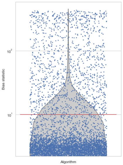
Figure 1. Distribution of bias statistic over all methods and parameter settings considered in this study, with the recommended thresholds: $[0,0]$ no SB, $(0,10]$ mild SB and $(10,\infty)$ strong SB. For examples of positions of final points for these three cases, see Figures 2a, 2b and  2c, respectively.

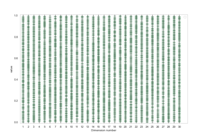
(a)

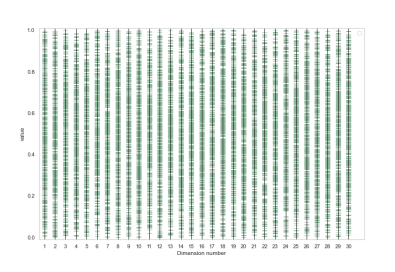
(b)

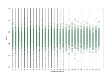
(c)

Figure 2. Examples of visible bias shown in parallel coordinate plots of the final results from $600$ runs of configurations with given parameter setting.

3. Emergence of structural bias in parameter space

Out of 10980 considered algorithm configurations, 4737 have showed at least some bias ($0<SB<10$) and 1343 algorithm configurations have showed strong bias ($SB\geq 10$), see Figure 1. Moreover, the kind of SB observed varies: the most obvious cases showing bias to the centre of the search domain and bias to the edges of the search domain (Figure 2).

The influence of the DE parameters, $F,C_{r}$ and $N$, is analysed by looking at the trends in the bias indicator for different crossover, mutation and correction strategies as shown in Figure 6a.

(a)

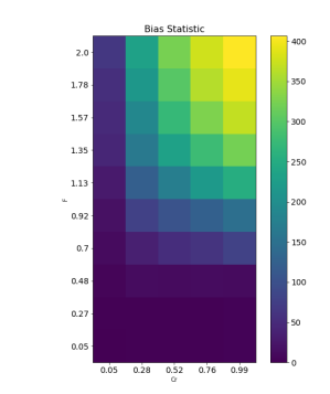
(b)

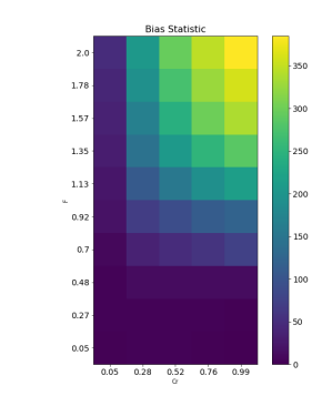
(c)

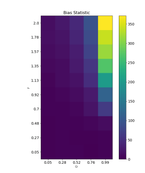
(d)

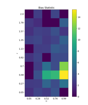
(e)

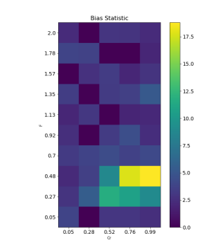
(f)

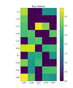
(g)

(h)

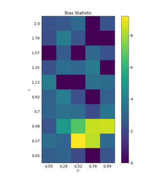
(i)

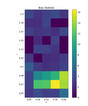
(j)

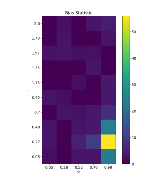
(k)

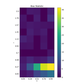
(l)

Figure 3. Bias indicators for different algorithms and population sizes for $F$ and $C_{r}$ settings. Brighter values indicate higher bias. Colour scale is not uniform across figures.

(a)

(b)

(c)

(d)

(e)

(f)

(g)

(h)

(i)

(j)

Figure 4. Bias indicator values for DE/curr-to-rand/1 configurations with p20 and p100 and different values of $F$ (shown on the vertical axis) and strategies — this mutation does not require a crossover and, thus, does not have $C_{r}$ parameter, see Section 2.2. Note a different colour scale indicating the strength of SB.

3.1. Analysis

Effect of $F$ and $C_{r}$

Setting of DE parameters can greatly affect the bias, depending on the algorithm configuration. Over all the results, we can split the bias trends in three groups regarding $F$ and $C_{r}$ settings:

• Group 1 where the bias is dependent on both $F$ and $C_{r}$ and where increasing either of the two increases the bias statistic.

• Group 2 where $F$ plays an important role in the bias, but $C_{r}$ does not.

• Group 3 where only specific combinations of $F$ and $C_{r}$ seem to cause (mild) bias.

For example, in the first group, in Figure 3a, there is a clear upwards trend in the bias indicator when either $F$ or $C_{r}$ value increases. In Figure 3d we can observe an increase in bias when $F$ increases, but the bias is only occurring for high $C_{r}$ settings (group 2). For some algorithm configurations, specific (lower) $F$ settings cause bias, such as in Figure 3e and Figure 3f (group 3). The bias in group 3 occurs mostly around $C_{r}=0.76$ and $F=0.48$. There are also configurations that do not show any clear bias pattern for $F$ and $C_{r}$ settings, such as in Figure 3g

In the cases of DE/curr-to-rand/1 there is no crossover operator, but we can see clear trends in different $F$ values and different correction strategies (Figure 4). For example, when using a COTN strategy low $F$ settings cause considerable bias, while very high $F$ settings only cause mild bias. For DE/curr-to-rand/1 with saturation strategy we can observe that both low and high $F$ values cause strong bias and only $F=0.92$ shows little bias (Figure 4d).

For the following algorithms (Group 1), only low $C_{r}$ and $F$ settings ($<0.48$) should be used to avoid bias (all sat-configurations, irrespective of population size):

• DE/rand-to-best/bin,

• DE/rand-to-best/exp,

• DE/rand/2/bin,

• DE/rand/2/exp,

• DE/curr-to-best/1/bin,

• DE/curr-to-best/1/exp,

• DE/best/1/bin,

• DE/best/2/bin, DE/best/2/exp,

• DE/best/1/exp.

Effect of population size

A larger population size slightly increases the structural bias as can be seen for example in Figure 4 when comparing p20-mir and p100-mir. This behaviour is consistent over all configurations that show mild or strong bias. See also Figures 3a, 3b, 3c.

Effect of mutation

In comparison with the other algorithm configuration settings, the choice of mutation operator has only little effect on the structural bias. Over all configurations, we can say that rand-to-best/2 shows a slightly stronger bias than the other mutation operators.

Effect of crossover

Crossover has a strong effect on the bias, we see that for bin crossover the bias statistic is consistently higher than for exp crossover. The $F$ and $C_{r}$ settings also have a different influence when using either binary or exponential crossover as can be seen in Figures 3c, 3d

Effect of strategy

The correction strategy has the strongest influence on the bias statistic. We can observe that sat strategy causes overall the most bias by far (Figures 3a, 3e and Figures 3b, 3f). Also strategy mirror and uniform cause strong bias in combination with mutation operator current-to-rand/1.

3.1.1. On recommended parameters settings

Accumulated experience of heuristic optimisation community has resulted in a number of publications that provide typical DE parameter settings for the use by general practitioners:

• $F\in[0.5,0.9]$ and $C_{r}\in[0.8,1]$, $p=10n$, where $n$ is problem dimensionality (Liu and Lampinen, 2005);

• $F\in\{0.5,0.9\}$, $C_{r}\in\{0.1,0.5,0.9\}$ and $p=50$ (Das and Suganthan, 2011);

• (Zaharie, 2002) has instead investigated the inter-relationship among parameters $F$ and $Cr$, and discovered an optimal tuning of the crossover rate as a function of the scale factor;

We have selected values from our algorithmic setup closest to these recommendations ($F\in\{0.48,0.92\}$, $C_{r}\in\{0.05,0.52,0.999\}$, $p\in\{20,100\}$) and ranked all considered configurations according the strength of structural bias – see Top 5s of such ranking in Tables 1, 2, per strategy. Since DE/curr-to-rand/1 does not require mutation, we consider it separately, see Table 3.

The general conclusion of this exercise is that considered configurations with COTN, dis, mir and recommended parameter setting, result in at most mild structural bias which is attained for not-necessarily uttermost values of recommended parameters. Meanwhile, as stated previously, sat, tor and uni generally result in a stronger SB. For recommended parameter settings, these strategies deliver at most strong SB for cases of DE/rand/2/$\star$, DE/best/$\star$ and DE/curr-to-best/1/$\star$, for sat, tor and uni, respectively. The case of DE/curr-to-rand/1, also appears to be strongly biased with COTN and uni.

Thus, general practitioners should avoid specific recommended parameter values if they choose sat, tor and uni strategies. The remaining strategies, should be used with care due to a possibility of mild SB.

Table 1. Top 5s of highest structural bias statistic scores among configurations with COTN, dis and mir strategies and parameter values in $F\in\{0.48,0.92\}$, $C_{r}\in\{0.05,0.52,0.999\}$, $p\in\{20,100\}$ closest to the recommended values.

configuration	p	F	$\mathbf{C_{r}}$	score
DE/curr-to-best/1/exp-COTN	100	0.483	0.99	26.36
DE/curr-to-best/1/bin-COTN	20	0.483	0.99	25.86
DE/curr-to-best/1/bin-COTN	20	0.483	0.52	24.98
DE/curr-to-best/1/bin-COTN	100	0.483	0.52	22.66
DE/curr-to-best/1/exp-COTN	20	0.483	0.99	20.68
DE/curr-to-best/1/bin-dis	100	0,916	0,99	4,67
DE/rand-to-best/2/exp-dis	20	0,916	0,05	4,46
DE/rand/2/bin-dis	20	0,916	0,99	4,37
DE/best/1/exp-dis	20	0,483	0,05	4,15
DE/rand/2/bin-dis	20	0,483	0,99	4,08
DE/best/2/exp-mir	20	0.483	0.99	5.44
DE/rand/2/bin-mir	100	0.483	0.52	4.84
DE/best/1/bin-mir	20	0.916	0.05	4.66
DE/best/2/exp-mir	100	0.916	0.52	4.61
DE/rand-to-best/2/exp-mir	100	0.483	0.52	4.11

Table 2. Top 5s of highest structural bias statistic scores among configurations with sat, tor and uni strategies and parameter values in $F\in\{0.48,0.92\}$, $C_{r}\in\{0.05,0.52,0.999\}$, $p\in\{20,100\}$ closest to the recommended values.

configuration	p	F	$\mathbf{C_{r}}$	score
DE/rand/2/exp-sat	20	0.916	0.99	174.85
DE/rand/2/bin-sat	100	0.916	0.99	171.71
DE/rand/2/exp-sat	100	0.916	0.99	171.60
DE/rand/2/bin-sat	20	0.916	0.99	165.99
DE/rand/2/bin-sat	20	0.916	0.52	163.24
DE/best/1/bin-tor	20	0.483	0.99	21.23
DE/best/2/bin-tor	20	0.483	0.99	20.11
DE/best/1/exp-tor	20	0.483	0.99	15.15
DE/best/2/bin-tor	100	0.483	0.99	13.51
DE/best/2/exp-tor	20	0.483	0.99	12.04
DE/curr-to-best/1/exp-uni	20	0.483	0.99	35.27
DE/curr-to-best/1/bin-uni	20	0.483	0.99	32.20
DE/curr-to-best/1/bin-uni	20	0.483	0.52	31.93
DE/curr-to-best/1/bin-uni	100	0.483	0.99	31.27
DE/curr-to-best/1/exp-uni	100	0.483	0.99	24.15

Table 3. Top 5s of highest structural bias statistic scores among configurations with curr-to-rand mutation and parameter values in $F\in\{0.48,0.92\}$, $p\in\{20,100\}$ closest to the recommended values.

configuration	p	F	score
DE/curr-to-rand/1-uni	100	0.483	91.60
DE/curr-to-rand/1-COTN	100	0.483	87.86
DE/curr-to-rand/1-COTN	20	0.483	87.08
DE/curr-to-rand/1-uni	29	0.483	81.74
DE/curr-to-rand/1-mir	100	0.483	79.23

3.1.2. Comparison with previous results

It is worth noting that configurations labelled biased with the graphical ‘parallel coordinate’ approach in (Caraffini et al., 2019) for a fixed parameter setting, have now been confirmed to be biased. An interesting case is
DE/current-to-best/1/bin with dis for all three population size. Indeed, it appears to be mildly biased via visual inspection (Caraffini et al., 2019) while our tests confirm the formation of a high structural bias.

4. Emergence of structural bias in time

Next to the emergence of SB in the parameter space, we have analysed a subset of algorithm configurations to investigate how the bias emerges over time, e.g. how the bias grows or shrinks after each evaluation.

For such analysis, each algorithm configuration is run for $300000$ fitness evaluations and $100$ runs (with different random seeds). We track SB by calculating the bias statistic using the active population of all $100$ runs for every evaluation.

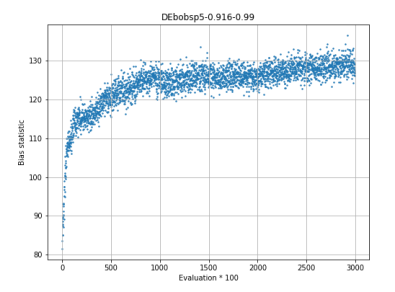
(a)

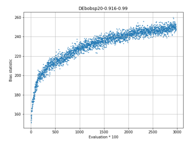
(b)

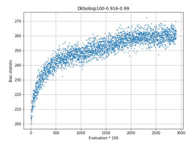
(c)

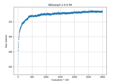
(d)

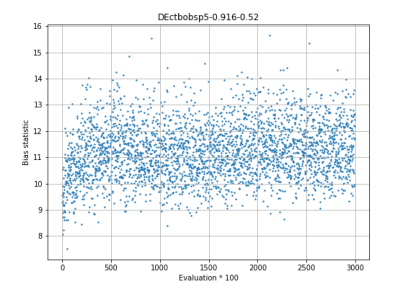
(e)

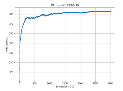
(f)

Figure 5. Examples of bias emerging over time (fitness evaluations) for different algorithm configurations.

4.1. Analysis

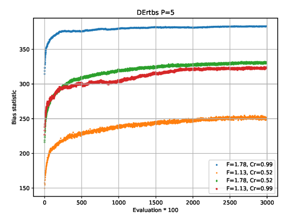
(a)

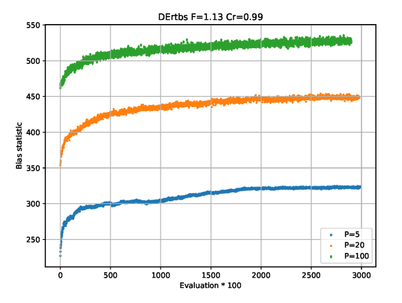
(b)

Figure 6. Examples of bias emerging over time (fitness evaluations) for different population sizes of DErtbs in Figure 6b and different $F$ and $C_{r}$ settings (Figure 6a).

In Figure 5 we can see the bias emerging over time for a selection of $6$ different algorithm configurations and population sizes. The selected algorithms use sat strategy, as these algorithms clearly show the most bias and are therefore of the highest interest to analyse.

We can observe that in all cases the algorithm starts unbiased. This is expected, since the initial population should be randomly uniform. After only a few evaluations though, the bias becomes evident and quickly climbs following a logarithmic curve. Even for cases with less bias, such as the DE/current-to-best/1/bin-p5-sat (Figure 5e), there is a clear trend starting at 0 and growing to an average of $11$ SB (i.e. the lower end of strong SB, following the definition above). In all plots we can also clearly see some degree of noise (roughly the same degree of noise in all cases, note that y-axes scale is different per figure). This noise is likely due to the stochastic nature of the experiment. It is also clear that if statistical bias manifests itself at some point in time, it does not disappear in the subsequent stages of evolution

When analysing different $F$ and $C_{r}$ settings over time for a configuration with saturation strategy, we can observe similar trends over time (Figure 6a). Higher $F$ and $C_{r}$ settings increase the bias reached over time. The slope of the curves however is only slightly affected. It is also clear that in this case both $F$ and $C_{r}$ have a similar importance for the bias statistic, increasing one and decreasing the other proportionally keeps the final bias stable. When we look at different population sizes (Figure 6b), we can observe a clear difference between sizes $5$, $20$ and $100$. This can be explained by the fact that the statistical test is performed on larger sample sizes for bigger populations ($p\times 100$), and does not necessarily mean that large populations also contribute to more bias.

5. Conclusions and future work

The total of $10980$ DE algorithm configurations with various parameter settings have been analysed for presence of structural bias. It has been shown that a significant number of these configurations (almost $1$ in $5$) show strong structural bias, indicated by an Anderson-Darling based statistical test (bias statistic $>10$). With many DE configurations show strong bias even within the ranges of originally proposed parameter settings $F$ and $C_{r}$. The saturation strategy stands out as one of the parameters that cause most bias, but also configurations like DE/best/1/bin-tor and DE/curr-to-best/1/exp-uni show significant structural bias.
Both $F$ and $C_{r}$ settings influence the emergence of structural bias. Generally speaking, high $F$ and $C_{r}$ values cause more bias than low values, however there are exceptions like the DE/curr-to-rand/1, where $F=0.05$ causes most structural bias in all cases.

Next to the effects of different configuration settings, the emergence of bias is measured over time (fitness evaluations). From the observations on these experiments it can be concluded that each algorithm configuration initially starts unbiased (with an initial population), but once structural bias starts to appear in the population it will only grow stronger during the remaining evaluations.

Our future research will concentrate on a finer analysis of structural bias in DE with an improved measure to find other less evident types of bias, with a smaller sample size. Moreover, we will continue looking for factors that give rise to SB.

- (1)
- (2)
- Barnsley (1988) Michael Barnsley. 1988. Fractals everywhere. Academic Press.
- Benjamini and Yekutieli (2001) Yoav Benjamini and Daniel Yekutieli. 2001. The Control of the False Discovery Rate in Multiple Testing under Dependency. The Annals of Statistics 29, 4 (2001), 1165–1188.
- Caraffini and Iacca (2020) Fabio Caraffini and Giovanni Iacca. 2020. The SOS Platform: Designing, Tuning and Statistically Benchmarking Optimisation Algorithms. Mathematics 8, 5 (May 2020), 785. https://doi.org/10.3390/math8050785
- Caraffini and Kononova (2019) Fabio Caraffini and Anna V. Kononova. 2019. Structural bias in differential evolution: A preliminary study. AIP Conference Proceedings 2070, 1 (2019), 020005. https://doi.org/10.1063/1.5089972
- Caraffini et al. (2019) Fabio Caraffini, Anna V. Kononova, and David W. Corne. 2019. Infeasibility and structural bias in differential evolution. Information Sciences 496 (2019), 161–179. https://doi.org/10.1016/j.ins.2019.05.019
- D’Aniello (2017) Emma D’Aniello. 2017. Non-self-similar sets in [0,1]N of arbitrary dimension. J. Math. Anal. Appl. 456, 2 (2017), 1123–1128. https://doi.org/10.1016/j.jmaa.2017.07.046
- D’Aniello and Steele (2019) Emma D’Aniello and Timothy H. Steele. 2019. Attractors for classes of iterated function systems. European Journal of Mathematics 5, 1 (2019), 116–137. https://doi.org/10.1007/s40879-018-0280-7
- Das et al. (2016) Swagatam Das, Sankha Subhra Mullick, and P.N. Suganthan. 2016. Recent advances in differential evolution – An updated survey. Swarm and Evolutionary Computation 27 (2016), 1 – 30. https://doi.org/10.1016/j.swevo.2016.01.004
- Das and Suganthan (2011) Swagatam Das and Ponnuthurai Nagaratnam Suganthan. 2011. Differential Evolution: A Survey of the State-of-the-Art. IEEE Trans. Evol. Comput. 15, 1 (2011), 4–31. https://doi.org/10.1109/TEVC.2010.2059031
- Frühwirth (1998) Thom Frühwirth. 1998. Theory and practice of constraint handling rules. The Journal of Logic Programming 37, 1-3 (1998), 95–138.
- Hanster and Kerschke (2017) Christian Hanster and Pascal Kerschke. 2017. flaccogui: Exploratory Landscape Analysis for Everyone. In Proceedings of the 19th Annual Conference on Genetic and Evolutionary Computation (GECCO) Companion (Berlin, Germany) (GECCO ’17). ACM, 1215 – 1222. https://doi.org/10.1145/3067695.3082477
- Kerschke and Trautmann (2019) Pascal Kerschke and Heike Trautmann. 2019. Comprehensive Feature-Based Landscape Analysis of Continuous and Constrained Optimization Problems Using the R-package flacco. In Applications in Statistical Computing – From Music Data Analysis to Industrial Quality Improvement, Nadja Bauer, Katja Ickstadt, Karsten Lübke, Gero Szepannek, Heike Trautmann, and Maurizio Vichi (Eds.). Springer, 93 – 123. https://doi.org/10.1007/978-3-030-25147-5_7
- Kim et al. (2007) H. Kim, J. Chong, K. Park, and D. A. Lowther. 2007. Differential Evolution Strategy for Constrained Global Optimization and Application to Practical Engineering Problems. IEEE Transactions on Magnetics 43, 4 (April 2007), 1565–1568. https://doi.org/10.1109/TMAG.2006.892100
- Kononova et al. (2020a) Anna V. Kononova, Fabio Caraffini, and Thomas Bäck. 2020a. Differential evolution outside the box results. https://arxiv.org/abs/2004.10489.
- Kononova et al. (2020b) Anna V. Kononova, Fabio Caraffini, Hao Wang, and Thomas Bäck. 2020b. Can Compact Optimisation Algorithms Be Structurally Biased?. In Parallel Problem Solving from Nature – PPSN XVI, T. Bäck, M. Preuss, A. Deutz, H. Wang, C. Doerr, M. Emmerich, and H. Trautmann (Eds.). Springer International Publishing, Cham, 229–242. https://doi.org/10.1007/978-3-030-58112-1_16
- Kononova et al. (2020c) Anna V. Kononova, Fabio Caraffini, Hao Wang, and Thomas Bäck. 2020c. Can Single Solution Optimisation Methods Be Structurally Biased?. In 2020 IEEE Congress on Evolutionary Computation (CEC). IEEE, Glasgow, 1–9. https://doi.org/10.1109/CEC48606.2020.9185494
- Kononova et al. (2015) Anna V. Kononova, David W. Corne, Philippe De Wilde, Vsevolod Shneer, and Fabio Caraffini. 2015. Structural bias in population-based algorithms. Information Sciences 298 (2015), 468–490. https://doi.org/10.1016/j.ins.2014.11.035
- Leguizamón and Coello (2006) Guillermo Leguizamón and Carlos A. Coello Coello. 2006. Boundary Search for Constrained Numerical Optimization Problems in ACO Algorithms. In Ant Colony Optimization and Swarm Intelligence, Marco Dorigo, Luca Maria Gambardella, Mauro Birattari, Alcherio Martinoli, Riccardo Poli, and Thomas Stützle (Eds.). Springer Berlin Heidelberg, Berlin, Heidelberg, 108–119. https://doi.org/10.1007/11839088_10
- Lehre and Witt (2012) Per Kristian Lehre and Carsten Witt. 2012. Black-Box Search by Unbiased Variation. Algorithmica 64, 4 (2012), 623–642. https://doi.org/10.1007/s00453-012-9616-8
- Liu and Lampinen (2005) J. Liu and J. Lampinen. 2005. A Fuzzy Adaptive Differential Evolution Algorithm. Soft Computing 9, 6 (01 Jun 2005), 448–462. https://doi.org/10.1007/s00500-004-0363-x
- Mersmann et al. (2011) Olaf Mersmann, Bernd Bischl, Heike Trautmann, Mike Preuss, Claus Weihs, and Günter Rudolph. 2011. Exploratory landscape analysis. In Proceedings of the 13th annual conference on Genetic and evolutionary computation. 829–836. https://doi.org/10.1145/2001576.2001690
- Miettinen (1999) Kaisa Miettinen (Ed.). 1999. Evolutionary Algorithms in Engineering and Computer Science: Recent Advances in Genetic Algorithms, Evolution Strategies, Evolutionary Programming, GE. John Wiley & Sons, Inc., New York, NY, USA.
- Storn and Price (1995) Rainer Storn and Kenneth Price. 1995. Differential Evolution - a Simple and Efficient Adaptive Scheme for Global Optimization over Continuous Spaces. Technical Report TR-95-012. ICSI.
- van Stein et al. (2021) Bas van Stein, Fabio Caraffini, and Anna V. Kononova. 2021. Emergence of Structural Bias in Differential Evolution - Source code & extended graphical results. https://doi.org/10.17632/pb2bdp2gkp.1
- Vermetten et al. (2021) Diederick Vermetten, Anna V. Kononova, Fabio Caraffini, Hao Wang, and Thomas Bäck. 2021. Is there Anisotropy in Structural Bias?. In Proceedings of the 2021 Genetic and Evolutionary Computation Conference Companion (Lille, France) (GECCO ’21 Companion). Association for Computing Machinery, New York, NY, USA. https://doi.org/10.1145/3449726.3463218
- Wolpert and Macready (1997) D. Wolpert and W. Macready. 1997. No free lunch theorems for optimization. IEEE Transactions on Evolutionary Computation 1 (1997), 67–82. Issue 1. https://doi.org/10.1109/4235.585893
- Zaharie (2002) D. Zaharie. 2002. Critical Values for Control Parameters of Differential Evolution Algorithm. In Proceedings of 8th International Mendel Conference on Soft Computing, R. Matuŝek and Pavel Oŝmera (Eds.). 62–67.