Joule-Thomson expansion for quantum corrected AdS-Reissner-Nördstrom black holes in Kiselev spacetime

Abstract

In this work we study the inversion temperature associated with the Joule-Thomson expansion from the thermodynamics of AdS-Reissner-Nördstrom black holes. We include quantum corrections in a cosmological fluid that can describe phantom dark matter or quintessence, both in a Kiselev scenario. The description of such physical systems involve numerical solutions and the results are presented as temperature-pressure plots for various values of the parameters of our model. We find non-zero minimum inversion temperatures as well as non-zero minimum pressures depending on the values of those parameters. Completing our study, we also find isenthalpic curves associated with black hole fixed mass processes.

I Introduction

Black hole thermodynamics is one of the most interesting topics in General Relativity. The history of the subject goes back to when Bekenstein proposed that the area of the black hole is proportional to its entropy Bekenstein:1973ur , followed by Hawking’s discovery that black holes radiate Hawking:1974sw . Since then, various thermodynamic properties have been attributed to black holes, such as internal energy, entropy, heat capacity, enthalpy, etc.

A little bit more than twenty years after such studies in Refs. Bekenstein:1973ur ; Hawking:1974sw the iconic work done by Witten, in Ref. Witten:1998zw , by using the new-found AdS/CFT correspondence, as proposed in Ref. Maldacena:1997re , relates the Hawking temperature achieved in a curved high-dimensional spacetime to the temperature of a super conformal Yang-Mills theory in a flat four-dimensional spacetime. Soon after Witten’s work the authors in Refs. Chamblin:1999tk ; Chamblin:1999hg studied the thermodynamic associated to a charged AdS black holes in the holographic context, and then opening up a multitude of possibilities to connect string and gauge theories through various types of black hole and its thermodynamics. It is worthwhile to mention that within holography the thermodynamics quantities are derived from the holographic renormalization of the on-shell euclidian action or the thermodynamics potentials.

Within general relativity context, some authors have proposed to associate mechanical pressure to black holes. For doing this, they considered that the cosmological constant is a thermodynamic variable that can be associated with the black hole pressure as shown in Refs. Kastor:2009wy ; Kubiznak:2012wp . In this way, applying the first law of thermodynamics, it is possible to deduce what would be the thermodynamic volume of a black hole, which is different from its physical volume. The existence of mechanical pressure in black holes allows us a better analogy with usual mechanical systems, such as thermal machines, where phase transitions occur naturally. For example, Johnson, in Ref. Johnson:2014yja , calculates the efficiency rate of a black hole, considering it to be a thermal machine in a Carnot cycle. Recently, another interesting example is presented by Ökcü and Aydıner in Ref. Okcu:2016tgt where they have studied a process similar to the Joule-Thomson process, in a black hole, and were able to calculate their temperature inversion curves. Traditionally, the Joule-Thomson effect aims to study the temperature variation when a gas goes through a process where its pressure changes. In this mechanical system, the temperature can increase or decrease, and for some gases a critical value can be found where a transition occurs when the temperature changes from increasing to decreasing, or the other way around. This can be represented mathematically by:

$$\mu=\left(\frac{\partial T}{\partial P}\right)_{H}\,,$$ (1)

which measures the temperature variation by the pressure variation in an isenthalpic process. Besides $\mu$ is Joule-Thomson coefficient and the mentioned inversion temperature is achieved by taking $\mu=0$ in above equation.

Since the work Okcu:2016tgt , several authors have proposed to study the Joule-Thomson process for different configurations of AdS black holes, in different gravitational theories Okcu:2017qgo ; Mo:2018rgq ; Lan:2018nnp ; Mo:2018qkt ; Cisterna:2018jqg ; Rizwan:2018mpy ; Chabab:2018zix ; Yekta:2019wmt ; Li:2019jcd ; Nam:2019zyk ; K.:2020rzl ; Bi:2020vcg . In most of these works, the result obtained follows a well-established pattern, which differs from the traditional result of a Van der Waals gas (see, e. g. Reif ).

The main purpose of this work is to study the effect of quantum corrections and cosmological fluids, such as quintessence and phantom dark energy, on the Joule-Thomson expansion in an AdS-Reissner-Nördstrom (AdS-RN) black hole.

Quantum corrections are relevant in the phenomenology of microscopic black holes. Its effects in a static black hole have been studied by Kazakov and Solodukhin Kazakov:1993ha , where the authors considered small deformations in the Schwarzschild metric due to the quantum fluctuations in the gravitational and matter fields. The effect of quantum corrections in phase transitions was studied in Ref. Lobo:2019put .

On the other hand, the introduction of a cosmological fluid is important because it is present both in the current and in the early universes. In order to incorporate cosmological fluids, we will use the Kiselev metric Kiselev:2002dx , where such matter can be described by an equation of state like $P=\,\omega\,\rho$. For instance, when $\omega=-2/3$, it can be said that the environment around the black hole is a kind of quintessence, and when $\omega<-1$ the environment is a kind of phantom dark energy Caldwell:1999ew .

This paper is divided as follows. In section II, we will present the AdS-Reissner-Nördstrom black hole with quantum corrections, surrounded by a Kiselev spacetime and make a brief study of its properties that are relevant to our study. In section III, we will calculate the mass of the black hole, its Hawking temperature and the inversion temperature of the Joule-Thomson expansion. In section IV, we will perform a numerical study of the inversion temperature and obtain their graphical solutions and the corresponding isenthalpic curves. Finally, in section V, we will present our conclusions.

II Quantum corrected charged AdS black hole surrounded by a Kiselev spacetime

The spacetime metric of the quantum corrected charged AdS black hole surrounded by a cosmological fluid is given by the following spherically symmetric metric,

$$ds^{2}=f(r)dt^{2}-f(r)^{-1}dr^{2}-r^{2}d\Omega^{2},$$ (2)

where $d\Omega^{2}$ is the solid angle, $d\theta^{2}+sin(\theta)^{2}d\phi^{2}$, and the horizon function is

$$f(r)=-\frac{2M}{r}+\frac{\sqrt{r^{2}-a^{2}}}{r}+\frac{r^{2}}{\ell^{2}}-{\frac{c}{r^{3\omega+1}}}+\frac{Q^{2}}{r^{2}}.$$ (3)

The parameter $M$ is the black hole mass, $a$ is related to the quantum correction, $\ell$ is the length scale of the asymptotically AdS spacetime, $c$ is a parameter related with the cosmological fluid, and $Q$ is the electric charge of the black hole.

Let us start by explaining why we have chosen the metric above and the origin of each term. First, we can highlight that M. Visser recently proposed that the Kiselev black hole can be generalized to a spacetime with N components whose relationship between energy and pressure, individually, is linear as shown in Ref. Visser:2019brz . That is, the spacetime for the generalized Kiselev black hole can be written as the metric (2) with

$$f(r)=\left(1-\sum_{i=i}^{N}\frac{c_{i}}{r^{3\omega_{i}+1}}\right).$$ (4)

Thus, choosing appropriate values for $\omega_{i}$ and $c_{i}$, one can reproduce all the terms of the proposed metric, except the mass term, because it receives a quantum correction. Nothing prevents us, then, from aggregating several terms whose equation of state is simply $P=\omega_{i}\rho$, although we must note that this relationship is built from an average in the energy-momentum tensor, as explained in the original article by Kiselev Kiselev:2002dx .

That said, we still have to explain why we chose the terms above. If we put $\omega=1/3$ and $c<0$, this term will be equivalent to an electric charge summing up with the last term in Eq. (3). The anti-de Sitter ($\omega=-1$), represented by the term $r^{2}/\ell^{2}$ in Eq. (3), is necessary for the definition of a mechanical pressure for the black hole Kastor:2009wy ; Kubiznak:2012wp . The novelty in this paper is the introduction of a cosmological fluid term in order to mimic quintessence, for instance, $\omega=-2/3,-1/6$, or phantom dark energy ($\omega=-4/3$).

The parameter $a$ is related to a deformation of the black hole mass due to quantum corrections and its origin can be found in Kazakov:1993ha . It is an independent parameter and for $a=0$ the metric reduces to the AdS-Reissner-Nordström metric surrounded by a cosmic fluid. In principle, it can assume any value as long as it is smaller than the radius of the event horizon, as expected, since it is a small correction to the black hole metric.

Before we study the thermodynamics of the system, let us make a little digression about the limits of the metric and the coordinate system. At the limit where the radius is small, we have

$$f\rightarrow 1-\frac{2M}{r}-\frac{a^{2}}{2r^{2}}+\frac{Q^{2}}{r^{2}}$$ (5)

as long as $3\omega+1<1$, which means that the black hole has two horizons, except in the extreme case where $4\,{M}^{2}-4\,{Q}^{2}+2\,a\leq 0$.

At the limit where the radius goes to infinity, we have

$$f\rightarrow\frac{r^{2}}{l^{2}}-\frac{c}{r^{3\omega+1}}$$ (6)

and the existence of a cosmological horizon depends on the values for $\omega$ and $c$. In the case where $\omega=-2/3$, the space will be asymptotically anti-de Sitter. This means that we must take a little care with our numerical analysis, since there is more than one horizon radius.

III Black hole thermodynamics and the inversion temperature

In this section we will provide a description of the black hole thermodynamics in our model and obtain the corresponding inversion temperature associated with the Joule-Thomson process. In this sense we will consider the mass of the black hole playing the role of the enthalpy, the area of the event horizon as the entropy and the cosmological constant will be associated with the black hole’s pressure Kubiznak:2012wp .

The first law of thermodynamics can be written as

$$dH=TdS+VdP+\Phi dQ,$$ (7)

and, since we are considering enthalpy and any non-mechanical work as constants,

$$0=T\left(\frac{dS}{dP}\right)_{H}+V.$$ (8)

To relate the above expression to the Joule-Thomson coefficient we must use some thermodynamic relations. Since the entropy is a state function,

$$dS=\left(\frac{\partial S}{\partial P}\right)_{T}dP+\left(\frac{\partial S}{\partial T}\right)_{P}dT$$ (9)

or, for an isenthalpic process,

$$\left(\frac{\partial S}{\partial P}\right)_{H}=\left(\frac{\partial S}{\partial P}\right)_{T}+\left(\frac{\partial S}{\partial T}\right)_{P}\left(\frac{\partial T}{\partial P}\right)_{H}.$$ (10)

Replacing this expression into Eq. (8), one has

$$0=\left[\left(\frac{\partial S}{\partial P}\right)_{T}+\left(\frac{\partial S}{\partial T}\right)_{P}\left(\frac{\partial T}{\partial P}\right)_{H}\right]+V.$$ (11)

Finally, using the Maxwell relation $(\partial S/\partial P)_{T}=-(\partial V/\partial T)_{P}$ and the definition for specific heat $C_{p}=T(\partial S/\partial T)_{P}$, one can substitute the above expression into (1) to find

$$\mu=\frac{1}{C_{p}}\left[T\left(\frac{\partial V}{\partial T}\right)_{P}-V\right],$$ (12)

and the inversion temperature occurs when $\mu=0$, i.e.,

$$T_{i}=V\left(\frac{\partial T}{\partial V}\right)_{P},$$ (13)

where the system changes from heating to cooling or the other way around.

Let us now proceed to study this process for the black hole. Fist of all, let us compute the black hole mass $M$, which is defined as a function of the location of its horizon $r_{+}$, trough the largest root of $f(r_{+})=0$, before any cosmological horizon. Then by using Eq. (3), one gets

$$f(r_{+})=0\Rightarrow M=\frac{1}{2}\left(\sqrt{r_{+}^{2}-a^{2}}-cr_{+}^{-3\omega}+\frac{r_{+}^{3}}{\ell^{2}}+\frac{Q^{2}}{r_{+}}\right)\,,$$ (14)

with $M$ interpreted as the enthalpy of the system.

In order to compute the entropy of the quantum-corrected Schwarzschild black hole in Kiselev spacetime, one can see in Ref. Shahjalal:2019pqb that this entropy is the same as Hawking-Bekenstein entropy, so that

$$S=\frac{A}{4}\Leftrightarrow S=\frac{4\pi r^{2}_{+}}{4}\Leftrightarrow r_{+}=\sqrt{\frac{S}{\pi}}\,.$$ (15)

Regarding our last thermodynamics variable, the pressure, we will consider it as related with the cosmological constant. Thus, the pressure has the following form Kubiznak:2012wp :

$$P=\frac{3}{8\pi\ell^{2}}\,,$$ (16)

Replacing Eqs. (15) and (16) in Eq. (14), one has:

$$M=\frac{1}{2\sqrt{\pi}}\left(\sqrt{{S}-\pi a^{2}}-c\pi^{\frac{3\omega+1}{2}}S^{-\frac{3\omega}{2}}+\frac{8PS^{3/2}}{3}+\pi Q^{2}S^{-1/2}\right).$$ (17)

The Hawking temperature is given by

$$T_{H}=\left(\frac{\partial M}{\partial S}\right)_{P,Q}\,,$$ (18)

and then one can write

$$T_{H}=\frac{1}{4\sqrt{\pi}}\left({\frac{1}{\sqrt{S-\pi a^{2}}}+8P\sqrt{S}}+3\frac{c\,\omega}{\sqrt{\pi}}\left(\frac{\pi}{S}\right)^{\frac{3\omega}{2}+1}-\frac{{\pi}\,Q^{2}}{S^{3/2}}\right)\,.$$ (19)

Using Eq. (15), one can rewrite the Hawking temperature as a function of the horizon radius, so that

$$T_{H}=\frac{1}{{4\pi}}\left({\frac{1}{\sqrt{r_{+}^{2}-a^{2}}}+3c\omega r_{+}^{-3\omega-2}+8\pi Pr_{+}-\frac{Q^{2}}{r_{+}^{3}}}\right)\,.$$ (20)

Now, using the numerical solutions to Eq. (14) written as $r_{+}=r_{+}(a,c,\omega,P,Q,M)$, in this equation, one gets the inversion temperature $T=T(a,c,\omega,P,Q,M)$. This result will be used in next section to construct the isenthalpic curves.

From the thermodynamics first law, Eq. (7), the thermodynamic volume of the black hole can be computed as

$$V=\left(\frac{\partial M}{\partial P}\right)_{S,Q}\Rightarrow V=\frac{4}{3}\pi r^{3}_{+}\,,$$ (21)

which gives us $r_{+}=(\frac{3V}{4\pi})^{1/3}$. Furthermore the Hawking temperature as a function of the black hole volume reads

$$T_{H}=\frac{1}{2\pi}{\left[{\left(\frac{6V}{\pi}\right)^{\frac{2}{3}}-4a^{2}}\right]^{-\frac{1}{2}}}+\frac{3\,\omega\,c}{4\pi}\left(\frac{3V}{4\pi}\right)^{-\omega-\frac{2}{3}}+P\left(\frac{6V}{\pi}\right)^{\frac{1}{3}}-\frac{Q^{2}}{3V}\,.$$ (22)

In order to get the inversion temperature, one can use its definition, so that

$$T_{i}=V\left(\frac{\partial T}{\partial V}\right)_{P}.$$ (23)

By using Eq. (22) and computing the inversion temperature, one has

$$T_{i}=-\frac{V^{2/3}}{\sqrt[3]{6}\pi^{5/3}\left(\left(\frac{6V}{\pi}\right)^{2/3}-4a^{2}\right)^{3/2}}-\frac{c\,\omega\left(3\omega+{2}\right)}{4\pi}\left(\frac{3V}{4\pi}\right)^{-\omega-\frac{2}{3}}+\sqrt[3]{\frac{6V}{\pi}}\frac{P}{3}+\frac{Q^{2}}{3V},$$ (24)

or, as a function of $r_{+}$,

$$T_{i}=\frac{2}{3}Pr_{+}-\frac{r_{+}^{2}}{12\pi\left(r_{+}^{2}-a^{2}\right)^{3/2}}-\frac{c\,\omega(3\omega+2)}{4\pi r_{+}^{2+3\omega}}+\frac{Q^{2}}{4\pi r_{+}^{3}}.$$ (25)

Finally, subtracting Eqs. (25) and (20), one gets

$${\frac{4r_{+}^{2}-3a^{2}}{\left(r_{+}^{2}-a^{2}\right)^{3/2}}+\frac{3\,c\,\omega(3\omega+5)}{r_{+}^{3\omega+2}}-\frac{6Q^{2}}{r_{+}^{3}}}+16\pi Pr_{+}=0.$$ (26)

This equation can be approximated for small values of $a$. In particular, for $c=0$, this equation can be solved analytically and implies the minimum inversion temperature ($P=0$), up to second order in $a$:

$$T_{min}=\frac{\sqrt{6}}{36\,\pi\,Q}\left[\,1+\left(\frac{a}{2\,Q}\right)^{2}\,\right]\,.$$ (27)

This equation shows the influence of the quantum correction on the minimum inversion temperature. If one takes the limit $a\to 0$ the result for $T_{min}$ presented in Ref. Okcu:2016tgt is recovered. For the complete model one has to resort to numerical methods which results will be presented in the next section.

IV Numerical results: Inversion temperature and Isenthalpic curves

In this section, we will present our numerical results for the inversion temperature, as well as the isenthalpic curves. Following the literature Kastor:2009wy ; Kubiznak:2012wp , we identify the black hole enthalpy with its mass. Then, the isenthalpic curves correspond to constant black hole masses in the $T-P$ phase diagram.

First, note that the Eq. (26) for $r_{+}$ does not have analytical solutions for arbitrary values of the parameters $a$, $c$, $\omega$, and $Q$. So, we solve it numerically, obtaining $r_{+}=r_{+}(a,c,\omega,Q,P)$. Then, we use these solutions in Eq. (20) to obtain the inversion temperature $T=T(a,c,\omega,Q,P)$. These results are presented in Figs. 1 - 6, where we plot $T$ as a function of the pressure $P$, for some choices of the parameters $a$, $c$, $\omega$, and $Q$.

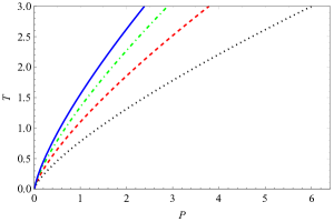
Figure 1: Inversion temperature as a function of the pressure for fixed $\omega=-1.0$, $c=0.1$, $a=0.1$ and the following charges $Q=1.0$ (black dotted), $Q=2.0$ (red dashed), $Q=3.0$ (green dot-dashed) and $Q=4.0$ (blue solid). Left panel: large range. We see that increasing the electric charge $Q$ increases the inversion temperature $T$ and its derivative. Right panel: small range. In this case we see the existence of non-zero pressures for $T=0$, and the dislocation of the curves for increasing electric charge $Q$.

In the left and right panels of Fig. 1, we have fixed the values of $\omega=-1$, $c=0.1$, $a=0.1$ and varied the electric charges from $Q=1.0$ to $Q=4.0$. In left panel of Fig. 1, we see as expected from the literature, for instance Okcu:2016tgt ; Okcu:2017qgo ; Mo:2018rgq ; Lan:2018nnp , that raising the black hole electric charge $Q$ the inversion temperature $T$ increases. Note that the inclusion of a small quantum correction $(a=0.1)$ does not change this pattern.

In the right panel of Fig. 1, we see that there are non-zero minimum values for the pressure $P$ at $T=0$. In general, for an AdS-RN black hole, there is a minimum temperature and not a minimum pressure; however, in our model, for non-zero values of the parameter $c$, the opposite occurs: the model no longer has a minimum temperature, but a minimum pressure. This behavior seems to be a feature of models with some kind of cosmological fluid, as seen in K.:2020rzl , where the cases $\omega=-1$ and $\omega=-1/3$ has been discussed for a Bardeen black hole.

In the right panel of Fig. 1, we also see that these non-zero values for the pressure increase with increasing electric charge $Q$. So, besides the increase of the derivative of the inversion temperature, the increase of the electric charge $Q$ also implies a small displacement of these curves in the direction of increasing pressure. In this panel, one also sees that for small values of the temperature and pressure the curves of constant charge intersect each other.

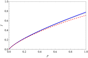
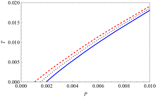
Figure 2: Inversion temperature as a function of the pressure for fixed $\omega=-1.0$, $c=0.1$, $Q=1.0$ and varying the quantum correction $a$ with values $0.1$ (solid blue), $0.3$ (dotted black) and $0.4$ (red dashed). Right panel: large range. Left panel: small range. In this case we see the existence of non-zero pressures for $T=0$, and the dislocation of the curves for decreasing quantum correction $a$.

In the left and right panels of Fig. 2, we plot the inversion temperature against the pressure for fixed values of $\omega=-1$, $c=0.1$, $Q=1.0$ and varying the quantum corrections from $a=0.1$ to $a=0.4$. In the left panel of Fig. 2, we see that the increase of the quantum correction decreases the inversion temperature. One should note that this happens for the high pressure regime. In the right panel of Fig. 2, we see that there are non-zero minimum values for the pressure $P$ at $T=0$, and that these non-zero values for the pressure decrease with increasing quantum correction $a$. So, besides the increase of the derivative of the inversion temperature, the increase of the quantum correction also implies a small dislocation of these curves in the direction of decreasing pressure. Comparing the left and right panels of Fig. 2, we conclude that these curves should intercept each other at intermediate values of the pressure.

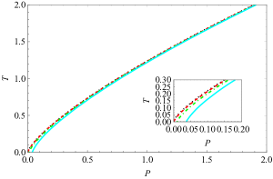
Figure 3: Inversion temperatures as a function of the pressure for fixed charge $Q=2.5$, quantum correction $a=0.1$ and $c=0.1$; we vary $\omega$ with the following values and $-1/6$ (black dotted), $-2/3$ (red dashed), $-1.0$ (green dot-dashed) and $-4/3$ (cyan solid).

In Fig. 3, we present the inversion temperature versus the pressure for fixed $Q=2.5$, $a=0.1$, $c=0.1$, and varying the quintessence $\omega=-1/6$, -2/3, -1, and -4/3. For increasing the absolute value of the quintessence we see a diminishing of the inversion temperature. In particular, it seems that for the phantom dark energy case $(\omega=-4/3)$ there might be a minimum inversion pressure.

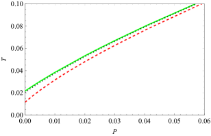
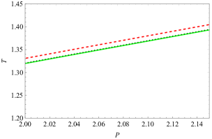
Figure 4: Inversion temperatures as a function of the pressure for fixed charge $Q=1.0$, quantum correction $a=0.1$, and $\omega=-1/6$. We vary $c$ with the following values $0.01$ (green solid), $0.10$ (black dotted), and $1.00$ (red dashed), in different scales (left and right panels) to show the details of this function.

In Fig. 4, we present the inversion temperature for fixed black hole charge, quantum correction, $\omega=-1/6$, and vary the cosmological fluid $c$ from 0.01 to 1.00. In the left panel, when we increase $c$ the pressure increases and the inversion temperature decreases. We also see a minimum inversion temperature for each value of $c$. In particular, when we increase $c$, we see that the minimum temperature decreases. In the right panel, the opposite occurs, which means, when we increase $c$ the pressure diminishes and the temperature increases. Comparing the two panels, we see that these curves should intercept each other for some intermediate pressure.

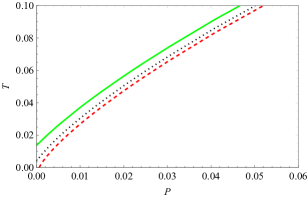
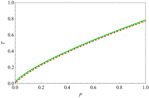
Figure 5: Inversion temperature as a function of the pressure for fixed charge $Q=1.0$ and quantum correction $a=0.1$. We set $\omega=-2/3$ and vary $c$ with the following values and $0.01$ (green solid), $0.10$ (black dotted), and $0.15$ (red dashed).

In Fig. 5, we show the inversion temperature for fixed black hole charge, quantum correction, $\omega=-2/3$, and vary the cosmological fluid $c$ from 0.01 to 0.15. In the left panel, when we increase $c$ the pressure increases and the inversion temperature decreases. We see minimum values for the inversion temperature only for $c$=0.01 and 0.10. In particular, for $c=0.15$ there is no minimum temperature but there is a minimum pressure. In the right panel, when we increase $c$ the pressure increases and the temperature decreases, as in the left panel. In this case we do not see the interception of the curves.

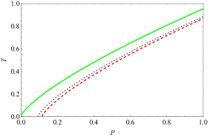
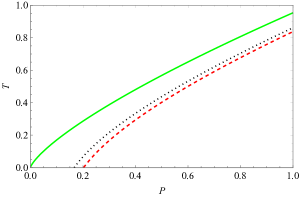
Figure 6: Inversion temperatures as a function of the pressure for fixed charge $Q=1.0$ and quantum correction $a=0.1$. Left panel: we set $\omega=-1$ and vary $c$ with the following values and $0.01$ (green solid), $0.80$ (black dotted), and $1.00$ (red dashed). Right panel: we set $\omega=-4/3$ and vary $c$ with the following values and $0.01$ (green solid), $0.80$ (black dotted), and $1.00$ (red dashed).

Now, we plot in Fig. 6, the inversion temperature for fixed quantum correction and black hole charge, and span the cosmological fluid $c$ from 0.01 to 1.0. In the left panel, we choose $\omega=-1$, while in the right panel, we took $\omega=-4/3$. In both cases, if we increase $c$ the pressure increases and the inversion temperature decreases. We see a minimum value for the inversion temperature only for $c$=0.01. On the other hand, for $c=0.80$ and 1.0 there are minimum values for the pressure. Notice that we do not see the interception of the curves for fixed $\omega$ and comparing the left and right panels one sees that if we increase the absolute value of $\omega$ the minimum pressure increases as well.

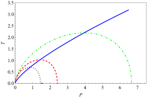
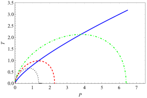
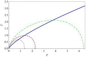
Figure 7: Isenthalpic curves for different values of the black hole mass, $M=1.8$ (black dotted), $M=2.0$ (red dashed), $M=3.0$ (green dot-dashed), for fixed $a=0.1,\,Q=1.0$, and $c=0.1$. The blue solid curves represent the inversion temperatures. Upper left panel: $\omega=-1/6$. Upper right panel: $\omega=-2/3$. Lower left panel: $\omega=-1$. Lower right panel: $\omega=-4/3$.

In order to obtain the isenthalpic curves for the black hole, we solve numerically the Eq. (14) for $r_{+}$ to get $r_{+}=r_{+}(a,c,\omega,P,Q,M)$, where we used the relation between the pressure and the AdS radius, Eq. (16). Applying this solution in Eq. (20) we achieve the profiles of the black hole mass in a plane $T-P$ for fixed sets of the other parameters. These results are shown in Fig. 7. Note that the isenthalpic curves are very similar for fixed values of $Q$, $a$ and $c$, varying $\omega$. However, there are small differences: in particular the values where the isenthalpic curves touch the pressure axis decrease as the absolute value of $\omega$ increases. Note that, as expected, the inversion temperature curves intercept the insenthalpics at their maxima. This can be understood as a numerical check of our analysis.

V conclusions

In this paper, we study the Joule-Thomson expansion for an AdS-RN black hole taking into account quantum corrections, in the scenario of a Kiselev metric. Within our model, we also considered the influence of a cosmic fluid. In order to mimic such a fluid, we have used equations of states given by $P=\omega\rho$, with $\omega$ assuming different values. For $\omega=-1$ one has the cosmological constant, for $\omega=-1/6$ or $-2/3$ one has quintessence, and phantom dark energy with $\omega=-4/3$. For each model, our goal was to study the behavior of the inversion temperature as a function of the pressure.

At this point it is worthwhile to make a first comment on the analysis of our results. If we consider only quantum corrections, without cosmological fluid $(c=0)$ or with a cosmological fluid that can be neglected $(c\to 0)$, we are able to perform a semi-analytical study and explicitly find an equation for the minimum inversion temperature as a function of the quantum correction parameter, at least in first order in $a$, as can be seen in Eq. (27). This result shows us that the model has a non-null minimum inversion temperature in this case ($c=0$ or $c\to 0$) .

When we considered quantum corrections and the cosmological fluid, or just the cosmological fluid, we were unable to find semi-analytical results for the inverson temperature, so we did a numerical study. In this case, we find that the introduction of the cosmological fluid not only changes the shape of the minimum temperature inversion curves, but can also lead to a minimum inversion pressure. This feature seems to be typical of models with cosmological fluids, considering that it was also found in K.:2020rzl , in the case where $\omega=-1/3$ for an AdS-RN Bardeen black hole. It is interesting to note how cosmological fluids can bring the minimum inversion temperature to zero.

In all the studied cases, the slope of the temperature inversion curves are strictly positive, however their shape varies with the values of the model parameters, for instance, the values for the quantum correction $a$ and the cosmological fluid $c$. In order to verify the consistency of our study, we also plotted the isenthalpic curves, showing that the temperature inversion curves intersect the isenthalpics at their maxima.

- (1) J. D. Bekenstein, “Black holes and entropy,” Phys. Rev. D 7 (1973), 2333-2346
- (2) S. W. Hawking, “Particle Creation by Black Holes,” Commun. Math. Phys. 43 (1975), 199-220 [erratum: Commun. Math. Phys. 46 (1976), 206]
- (3) E. Witten, “Anti-de Sitter space, thermal phase transition, and confinement in gauge theories,” Adv. Theor. Math. Phys. 2, 505-532 (1998) [arXiv:hep-th/9803131 [hep-th]].
- (4) J. M. Maldacena, “The Large N limit of superconformal field theories and supergravity,” Adv. Theor. Math. Phys. 2, 231-252 (1998) [arXiv:hep-th/9711200 [hep-th]].
- (5) A. Chamblin, R. Emparan, C. V. Johnson and R. C. Myers, “Charged AdS black holes and catastrophic holography,” Phys. Rev. D 60, 064018 (1999) [arXiv:hep-th/9902170 [hep-th]].
- (6) A. Chamblin, R. Emparan, C. V. Johnson and R. C. Myers, “Holography, thermodynamics and fluctuations of charged AdS black holes,” Phys. Rev. D 60, 104026 (1999) [arXiv:hep-th/9904197 [hep-th]].
- (7) D. Kastor, S. Ray and J. Traschen, “Enthalpy and the Mechanics of AdS Black Holes,” Class. Quant. Grav. 26 (2009), 195011 [arXiv:0904.2765 [hep-th]].
- (8) D. Kubiznak and R. B. Mann, “P-V criticality of charged AdS black holes,” JHEP 07 (2012), 033 [arXiv:1205.0559 [hep-th]].
- (9) C. V. Johnson, “Holographic Heat Engines,” Class. Quant. Grav. 31 (2014), 205002 [arXiv:1404.5982 [hep-th]].
- (10) Ö. Ökcü and E. Aydıner, “Joule–Thomson expansion of the charged AdS black holes,” Eur. Phys. J. C 77 (2017) no.1, 24 [arXiv:1611.06327 [gr-qc]].
- (11) Ö. Ökcü and E. Aydıner, Eur. Phys. J. C 78 (2018) no.2, 123 [arXiv:1709.06426 [gr-qc]].
- (12) J. X. Mo, G. Q. Li, S. Q. Lan and X. B. Xu, “Joule-Thomson expansion of -dimensional charged AdS black holes,” Phys. Rev. D 98 (2018) no.12, 124032 [arXiv:1804.02650 [gr-qc]].
- (13) S. Q. Lan, “Joule-Thomson expansion of charged Gauss-Bonnet black holes in AdS space,” Phys. Rev. D 98 (2018) no.8, 084014 [arXiv:1805.05817 [gr-qc]].
- (14) J. X. Mo and G. Q. Li, “Effects of Lovelock gravity on the Joule–Thomson expansion,” Class. Quant. Grav. 37 (2020) no.4, 045009 [arXiv:1805.04327 [gr-qc]].
- (15) A. Cisterna, S. Q. Hu and X. M. Kuang, “Joule-Thomson expansion in AdS black holes with momentum relaxation,” Phys. Lett. B 797 (2019), 134883 [arXiv:1808.07392 [gr-qc]].
- (16) A. Rizwan C.L., N. Kumara A., D. Vaid and K. M. Ajith, “Joule-Thomson expansion in AdS black hole with a global monopole,” Int. J. Mod. Phys. A 33 (2019) no.35, 1850210 [arXiv:1805.11053 [gr-qc]].
- (17) M. Chabab, H. El Moumni, S. Iraoui, K. Masmar and S. Zhizeh, “Joule-Thomson Expansion of RN-AdS Black Holes in gravity,” LHEP 02 (2018), 05 [arXiv:1804.10042 [gr-qc]].
- (18) D. Mahdavian Yekta, A. Hadikhani and Ö. Ökcü, “Joule-Thomson expansion of charged AdS black holes in Rainbow gravity,” Phys. Lett. B 795 (2019), 521-527 [arXiv:1905.03057 [hep-th]].
- (19) C. Li, P. He, P. Li and J. B. Deng, “Joule-Thomson expansion of the Bardeen-AdS black holes,” Gen. Rel. Grav. 52 (2020) no.5, 50 [arXiv:1904.09548 [gr-qc]].
- (20) C. H. Nam, “Heat engine efficiency and Joule–Thomson expansion of nonlinear charged AdS black hole in massive gravity,” Gen. Rel. Grav. 53 (2021) no.3, 30 [arXiv:1906.05557 [gr-qc]].
- (21) Rajani K. V, C. L. A. Rizwan, A. Naveena Kumara, D. Vaid and M. S. Ali, “Joule-Thomson Expansion of Regular Bardeen AdS Black Hole Surrounded by Static Anisotropic Quintessence Field,” [arXiv:2002.03634 [gr-qc]].
- (22) S. Bi, M. Du, J. Tao and F. Yao, “Joule-Thomson expansion of Born-Infeld AdS black holes,” Chin. Phys. C 45, no.2, 025109 (2021) [arXiv:2006.08920 [gr-qc]].
- (23) F. Reif, Fundamentals of statistical and thermal physics, McGraw-Hill, 1965.
- (24) D. I. Kazakov and S. N. Solodukhin, “On Quantum deformation of the Schwarzschild solution,” Nucl. Phys. B 429 (1994), 153-176 [arXiv:hep-th/9310150 [hep-th]].
- (25) V. B. Bezerra, I. P. Lobo, J. P. Morais Graça and L. C. N. Santos, “Effects of quantum corrections on the criticality and efficiency of black holes surrounded by a perfect fluid,” Eur. Phys. J. C 79, no.11, 949 (2019) [arXiv:1908.08140 [gr-qc]].
- (26) V. V. Kiselev, “Quintessence and black holes,” Class. Quant. Grav. 20, 1187-1198 (2003) [arXiv:gr-qc/0210040 [gr-qc]].
- (27) R. R. Caldwell, “A Phantom menace?,” Phys. Lett. B 545, 23-29 (2002) [arXiv:astro-ph/9908168 [astro-ph]].
- (28) M. Visser, “The Kiselev black hole is neither perfect fluid, nor is it quintessence,” Class. Quant. Grav. 37 (2020) no.4, 045001 [arXiv:1908.11058 [gr-qc]].
- (29) M. Shahjalal, “Thermodynamics of quantum-corrected Schwarzschild black hole surrounded by quintessence,” Nucl. Phys. B 940, 63-77 (2019)